18.117 Lecture Notes

Victor Guillemin and Jonathan Campbell

August 19, 2005

Chapter 1

Several Complex Variables

Lecture 1

Lectures with Victor Guillemin,Texts: Hormander: Complex Analysis in Several Variables Griffiths: Principles in Algebraic Geometry Notes on Elliptic Operators No exams, 5 or 6 HW’s. Syllabus (5 segments to course, 6-8 lectures each)

1. Complex variable theory on open subsets of Cn . Hartog, simply pseudoconvex domains, inhomogeneous C.R.

2. Theory of complex manifolds, Kaehler manifolds

3. Basic theorems about elliptic operators, pseudo-differential operators

4. Hodge Theory on Kaehler manifolds

5. Geometry Invariant Theory.

1 Complex Variable and Holomorphic Functions

U an open set in Rn, let C∞(U) denote the C∞ function on U . Another notation for continuous function: Let A be any subset of Rn , f ∈ C∞(A) if and only f ∈ C∞(U) with U ⊃ A, U open. That is, f is C∞ on A if it can be extended to an open set around it.

As usual, we will identify C with R2 by z �→ (x, y) when z = x + iy. On R2 the standard de Rham differentials are dx, dy. On C we introduce the de Rham differentials

dz = dx + idy dz = dx − idy

Let U be open in C, f ∈ C∞(U) then the differential is given as follows

∂f ∂f ∂f � dz + dz

� ∂f � dz − dz

�

df = dx + dy = + ∂x ∂y ∂x 2 ∂y 2i

1 � ∂f ∂f

� 1 � ∂f ∂f

�

= dz + + i dz2 ∂x

− i∂y 2 ∂x ∂y

If we make the following definitions, the differential has a succinct form

∂f 1 � ∂f ∂f

� ∂f 1

� ∂f ∂f

�

= = + i ∂z 2 ∂x

− i ∂y ∂z 2 ∂x ∂y

so ∂f ∂f

df = dz + dz. ∂z ∂z

We take this to be the definition of the differential operator.

3

Definition. f ∈ O(U ) (the holomorphic functions) iff ∂f /∂z = 0. So if f ∈ O(U ) then df = ∂f dz.∂z

Examples

1. z ∈ O(U )

2. f, g ∈ C∞(U ) then∂f ∂f ∂gf g = g + f

∂z ∂z ∂z

so if f, g ∈ O(U ) then f g ∈ O(U ).

3. By the above two, we can say z, z2 , . . . and any polynomial in z is in O(U ).

4. Consider a formal power series f (z) ∼ �∞ i where ai ≤ (const)R−i . Then if D = z < R}i=1 aiz | | {| |the power series converges uniformly on any compact set in D, so f ∈ C(D). And by term-by-term differentiation we see that the differentiated power series converges, so f ∈ C∞(D), and the differential w/ respect to z goes to 0, so f ∈ O(D).

15. a ∈ C, f (z) = z−a ∈ C∞(C − {a}).

Cauchy Integral Formula

Let U be an open bounded set in C, ∂U is smooth, f ∈ C∞(U ). Let u = f dz by Stokes

� � ∂f ∂f

f dz = du du = dz ∧ dz + dz ∧ dz ∂z ∂z∂U U

so � � � ∂f

f dz = du = dz ∧ dz. ∂z∂U U U

Now, take a ∈ U and remove Dǫ = z − a < ǫ}, and let the resulting region be Uǫ = U −Dǫ. Replace {| |f in the above by f . Note that (z − a)−1 is holomorphic. We get z−a

� f

� ∂f 1

dz = dz ∧ dz ∂Uǫ

z − a Uǫ ∂z z − a

Note: The boundary of U is oriented counter-clockwise, and the inner boundary Dǫ is oriented clockwise. When orientations are taken into account the above becomes

� f

� f (z)

� ∂f 1

dz − dz = dz ∧ dz (1.1) ∂U z − a ∂Dǫ

z − a Uǫ ∂z z − a

dz The second integral, with the change of coordinates z = a + ǫeiθ , dz = iǫeiθ , = idθ. This gives z−a

� f (z)

dz = i � 2π

f (a + e iθ)dθ. ∂Dǫ

z − a 0

Now we look at what happens when ǫ 0. Well, 1 z−a ∈ L1(U ), so by Lebesgue dominated convergence if →

we let Uǫ → U , and the integral remians unchanged. On the left hand side we get −if (a)2π, and altogether we have �

f �

∂f 1 2πif (a) = dz + dz ∧ dz

U z − a U ∂z z − a

In particular, if f ∈ O(U ) then � f

2πif (a) = dz ∂U z − a

Applications:

4

f ∈ C∞(U) ∩ O(U), take a z, z η then just rewriting

� f(η)

2πif(z) = dη ∂U η − z

If we let U = {D : z < R}. Then | |

k1 1 1 ∞

z=

η ηkη − z η �1 − z

� = �

η k=0

and since on boundary η = R, z < R so the series converges uniformly on compact sets, we get | | | |�

f(η) ∞

f(η)kdη = �

akz ak =

� dη

ηk+1 ∂U ζ − z

k=0 |η|=R

1 ∂k

or ak = f(0). This is the holomorphic Taylor expansion. k! ∂zk

Now if we take z z − a, D : z − a < R, f ∈ O(U) ∩ C∞(U) then | |

1 ∂k

f(z) = �

ak(z − a)k ak = f(a)k! ∂zk

We can apply this a prove a few theorems.

Theorem. U a connected open set in C. f, g ∈ O(U), suppose there exists an open subset V of U on which f = g. We can conclude f ≡ g, this is unique analytic continuation.

Proof. W set of all points a ∈ U where

∂kf ∂kg = k = 0, 1, . . .

∂zk (a)

∂zk

holds. Then W is closed, and we see that W is also open, so W = U .

Lecture 2

Cauchy integral formula again. U an open bounded set in C, ∂U smooth, f ∈ C∞(U), z ∈ U

1 �

f(η) 1 �

∂f 1 f(z) =

2πi ∂U η − zdη + (η)

η − zdη ∧ dη

2πi U ∂η

the second term becomes 0 when f is holomorphic, i.e. the area integral vanishes, and we get

1 �

f(η)f(z) = dη

2πi ∂U η − z

Now take D : z − a < ǫ, f ∈ O(D) ∩C∞(D), then | |� 2π1

f(a) = f(a + ǫe iθ)dθ 2π 0

More applications:

Theorem (Maximum Modulus Principle). U any open connected set in C, f ∈ O(U) then if f has a local maximum value at some point a ∈ U then f has to be constant.

| |

First, a little lemma.

5

�

Lemma. If f ∈ O(U) and Ref ≡ 0, then f is constant.

Proof. Trivial consequence of the definition of holomorphic.

Proof of Maximum Modulus Principle. Assume f(a) is positive (we can do this by a trivial normalizationoperation). Let u(z) = Re f . Now from above

2π1 �

f(a) = f(a + ǫe iθ)dθ 2π 0

The LHS is real valued and trivially 2π1

�f(a) = f(a)dθ

2π 0

we subtract the above 2 and we get

2π

0 = f(a) − u(a + ǫe θ)dθ. 0

When ǫ is sufficiently small, since a is a local maximum, the integral is greater than 0, f(a) = u(a + ǫeiθ) so Re f is constant in a neighborhood of a and we can normalize and assume Re f = 0 near a, so by analytic continuation f is constant on U .

Inhomogeneous CR Equation

Consider U an open bounded subset of C, ∂U a smooth boundary, g ∈ C∞(U). The Inhomogeneous CR equation is the following PDE: find f ∈ C∞(U) such that

∂f = g

∂z

The question is, does there exists a solution for arbitrary g? First, consider another, simpler version of CR with g ∈ C0

∞(C). Does there exists f ∈ C∞(C) such that ∂f/∂z = g?

Lemma. We claim the function f defined by the integral

1 �

g(η)f(z) =

η − zdη ∧ dη

2πi

is in C∞(C) and satisfies ∂f/∂z = g.

Proof. Perform the change of variables w = z − η, dw = −dη, d w = −dη and η = z − w then the integral above becomes �

g(z − w)dw ∧ d w = f(z)−

w

Now it is clear that f ∈ C∞(C), because if we take ∂/∂z, we can just keep differentiating under the integral. And now

∂g �

��∂g �

(η)z η∂f 1 ��∂¯ (z − w) 1 ∂¯

= dw ∧ d w = η − z

dη ∧ dη∂z

−2πi w 2πi

Let A = supp g, so A is compact, then there exists U open and bounded such that ∂U is smooth and A ⊂ U . For g ∈ C∞(U) write down using the Cauchy integral formula

1 �

g(η) 1 �

∂g (η)

dη ∧ dηg(z) = dη +

2πi ∂U η − z 2πi U ∂η η − z

On ∂U , g is identically 0, so the first integral is 0. For the second integral we replace A by the entire complex plane, so

1 �

∂g (η)

dη ∧ dηg(z) =

2πi C ∂η η − z

which is the expression for ∂f ∂z

6

Now, we want to get rid of our compactly supported criterion. Let U be bounded, ∂U smooth and g ∈ C∞(U), ∂f = g.∂z

Make the following definition1 �

g(η)f(z) :=

2πi U η − zdη ∧ dη

Take a ∈ U , D an open disk about a, D ⊂ U . Check that f ∈ C∞ on D and that ∂f/∂z = g on D. Since a is arbitrary, if we can prove this we are done. Take ρ ∈ C0

∞(U) so that ρ ≡ 1 on a neighborhood of D, then

1 � ρ(η)g(η) 1

� g(η)

f(z) = η − z

dη ∧ dη+ (1 − ρ)η − z

dη ∧ dη2πi 2πi � �� � � �� �

I II

The first term, I, is in C0∞(C), so I is C∞ on C and ∂I/∂z = ρg on C and so is equal to g D. We claim that

II D is in O(D). The Integrand is 0 on an open set containing D, so ∂II/∂z = 0 on D. |

|We conclude that ∂f(z)/∂z = g(z) on D. (The same result could have just been obtained by taking a

partition of unity)

Transition to Several Complex Variables

We are now dealing with Cn, coordinatized by z = (z1, . . . , zn), and zk = xk + iyk and dzk = dxk + idyk. Given U open in Cn , f ∈ C∞(U) we define

∂f 1 � ∂f ∂f

� ∂f 1

� ∂f ∂f

�

∂zk =

2 ∂xk − i

∂yk ∂zk =

2 ∂xk + i

∂yk

So the de Rham differential is defined by

�� ∂f ∂y

� � ∂f � ∂f ¯df dxi + dyi dzk + dzk := ∂f + ∂f = = ∂xi ∂yi ∂zk ∂zk

so df = ∂f + ∂f . Let Ω1(U) be the space of C∞ de Rham 1-forms, and u ∈ Ω1(U) then

u = u ′ + u ′′ = �

aidzi + �

bidzi ai, bi ∈ C∞(U)

we introduce the following notation

Ω1,0 = ��

akdzk, ak ∈ C∞(U)�

Ω0,1 = ��

bkdzk, bk ∈ C∞(U)�

and therefore there is a decomposition Ω1(U) = Ω1,0(U) ⊕ Ω0,1(U). We can rephrase a couple of the lines above in the following way: df = ∂f + ∂f , ∂f ∈ Ω1,0 , ∂f ∈ Ω0,1 .

Definition. f ∈ O(U) if ∂f = 0, i.e. if ∂f/∂zk = 0, ∀k. Lemma. For f, g ∈ C∞(U), ∂fg = f∂g + g∂f , thus fg ∈ O(U).

Obviously, z1, . . . , zn ∈ O(U). α1If α = (α1, . . . , αn), αi ∈ N, then zα = z1 . . . z

αn and zα ∈ O(C). Then n

α p(z) = �

aαz )∈ O(Cn

α ≤N| |

Even more generally, suppose we have the formal power series

αf(z) = �

aαz α

and aα ≤ CR−α1 . . . R−αn . Then let Dk : zk < Rk and D = then f(z) converges on D and 1 n| | | | D1 × · · · ×Dn uniformly on compact sets in D, and by differentiation we see that f ∈ O(D).

Definition. Let Di : z − ai < Rn, then open set D1 × · · · ×Dn is called a polydisk.| |

7

= = �

Lecture 3

Generalizations of the Cauchy Integral Formula

There are many, many ways to generalize this, but we will start with the most obvious

Theorem. Let D ⊆ Cn be the polydisk D = n where Di : zi < Ri and let f ∈ O(D) ∩C∞(D) then for any point a = (a1, . . . , an)

D1 × · · · ×D | |

� 1 �n �

f(z1, . . . , zn)f(a) = n

2πi (z1 − a1) . . . (zn − an) dz1 ∧ · · · ∧ dz

∂D1×···×∂Dn

Proof. We will prove by induction, but only for the case n = 2, the rest follow easily. We do the Cauchy Integral formula in each variable separately

1 �

f(z1, z2) 1 �

f(z1, z2)f(z1, a2) = dz1 f(a1, zn) = dz2

2πi ∂D2 z2 − z2 2πi ∂D2

(z1 − a1)

Then just plug the first into the second.

Applications: First make the following changes ai zi, zi ηi, then

� 1 �n �

f(η)f(z1, . . . , zn) = n

2πi (η1 − z1) . . . (ηn − zn) dη1 ∧ · · · ∧ dη

∂D1×···×∂Dn

As before in the single variable case we make the following replacements

1 1 1 1 zα �

(ηi − zi) η1 . . . ηn

� zi η1 . . . ηn ηα1 − ηi α

n we have uniform converge for z on compact subsets of D. So by the Lebesgue for η ∈ ∂D1 × · · · × ∂Ddominated convergence theorem

f(η)αf(z) = �

aαz aα =

� 1 �n �

ηα1+1 n+1 2πi . . . ηαndη1 ∧ · · · ∧ dη

nα 1

Theorem. U open in Cn , f ∈ O(U), a ∈ U and D a polydisk centered at a with D ⊆ U then on D we have

f(z) = �

aα(z1 − a1)α1 . . . (zn − an)

αn

α

(we will call this (∗) from now on)

Proof. Apply the previous little theorem to f(z − a).

1Note we can check by differentiation that the coefficients are aα = α!∂f/∂zα(a).

Theorem. U is a connected open set in Cn with f, g ∈ O(U). If f = g on an open subset V ⊂ U then f = g on all of U .

Proof. As in one dimension.

Theorem (Maximum Modulus Principle). U is a connected open set in Cn , f ∈ O(U). If |f | achievesa local maximum at some point a ∈ U then f is constant

Proof. Left as exercise.

As a reminder:

8

Theorem. Let g ∈ C0∞(C) then if f is the function

1 �

g(η)f(z) =

2πi C η − zdη ∧ dη

then f ∈ C∞(C) and ∂f/∂z = g.

What about the n-dimensional case? That is, given hi ∈ C0∞(Cn), i = 1, . . . , n does there exist f ∈

C∞(Cn) such that ∂f = hi, i = 1, . . . , n?∂zi

There clearly can’t always be a solution because we have the integrability conditions

∂hi ∂hj=

∂zj ∂zi

Theorem (Multidimensional Inhomogeneous CR equation). If the hi’s satisfy these integrability conditions then there exists an f ∈ C∞(Cn) with ∂f/∂zi = hi. And in fact such a solution is given by

1 �

h1(η1, z2, . . . , zn)f(z1, . . . , zn) =

2πi C (η1 − z1) dη1 ∧ dη1

Proof. This just says for get about everything except the first variable. Clearly f ∈ C∞(Cn) and ∂f/∂z1 = h1. Now ∂f/∂zi we compute under the integral sign and we get

∂ 1 h1(η1, z2, . . . , zn)

ηi − zi ∈ L′(η1)

∂zi

(so it is legitimate to differentiate under the integral sign). Now

∂f =

1 � ∂h1

(η1, z2, . . . , zn) dη1 ∧ dη1

∂zi 2πi ∂zj η1 − z1 1

=

� ∂hj

(η1, z2, . . . , zn) dη1 ∧ dη1

2πi ∂η1 η1 − z1 = hj(z1, . . . , zn)

The second set is by integrability conditions, and the lat is by the previous lemma. QED.

Let K ⋐ Cn be a compact st. Suppose Cn −K is connected. Suppose hi ∈ C0∞(Cn) are supported in K.

Theorem. If f is the function (∗) then supp f ⊆ K(unique to higher dimension). So not only do we havea solution to the ICR eqn, it is compactly supported.

Proof. By (∗) f(z1, . . . , zn) is identically 0 when (zi) ≫ 0, i > 1, because hi is compactly supported. Also,since supphi ⊆ K and ∂f/∂zi = hi we have that ∂f/∂zi = 0 on Cn −K, so f ∈ O(Cn −K). The uniqueness of analytic continuation we have f ≡ 0 on Cn −K (used that Cn −K is connected)

Theorem (Hartog’s Theorem). Let K ⋐ U , U ⊂ Cn is open and connected. Suppose that U − K is connected. Let f ∈ O(U − K) then f extends holomorphically to all of U . THIS IS A PROPERTY SPECIFIC TO HIGHER DIMENSIONAL SPACES.

Proof. Let K1 ⋐ U so that K ⊂ Int K1, U −K1 is connected. Choose ϕ ∈ C∞(Cn) such that ϕ ≡ 1 on K and suppϕ ⊂ Int K1. Let �

(1 − ϕ)f on U −K v =

0 on K

then v ∈ C∞(U). And v ≡ f on U − K. hi = ∂ v, i = 1, . . . , n. One U − K1, v = so ∂zi f ∈ O(U − K1)

∂ ∂hjhi = ∂¯ f on U −K1 and f is holomorphic, so this is 0, thus hi ∈ C0∞(Cn), supphi ⊆ K1 and ∂hi = zi ∂¯ zjzj ∂¯ ,

so ∃w ∈ C0∞(Cn) such that ∂w = hi and suppw ⊆ K1. Take g = v − w so w ≡ 0 on Cn − K, v = f on ∂zi

Cn −K1, so g = f on Cn −K and by construction

∂g ∂v ∂w ∂ = = hi −

∂zi ∂zi −∂zi ∂zi

w = 0

and g = f on U − K1, f ∈ C∞(U − K), since U − K connected, by uniqueness of analytic so g ∈ O(U) continuation g = f on U −K, so g is holomorphic continuation of f onto all of U .

9

2

Lecture 4

Applying Hartog’s Theorem

Let X ⊂ Cn be an algebraic variety, codC X = 2. And suppose f ∈ O(Cn −X). Then f extends holomor­phically to f ∈ O(Cn).

Sketch of Proof : Cut X by a complex plane (P = C2) transversally. Then f P ∈ O(P − {p}) so by hartog, f P ∈ O(P ). Do this argument for all points, so f has to be holomorphic on

|f ∈ O(Cn).|

We have to be a little more careful to actually prove it, but this is just an example of how algebraic geometers use this.

Dolbeault Complex and the ICR Equation

Let U be an open subset of Cn , ω ∈ Ω1(U), then we discussed how Ω1(U) = Ω1,0 ⊕ Ω0,1 . There is a similar story for higher degree forms. Take r > 1, p + q = r. Then ω ∈ Ωp,q (U) if ω is in the following form

ω = �

fI,J dzI ∧ dzJ fI,J ∈ C∞(U)

and dzI = , dzJ = d¯ zjq are standard multi-indices. Thendzi1 ∧ · · · ∧ dzip

zj1 ∧ · · · ∧ d¯�

Ωp,q(U)Ωr = p+q=r

Now suppose we have ω ∈ Ωp,q (U), ω = � fI,J dzI ∧ dzJ then the de Rham differential is written as follows

dw = �

dfIJ ∧ dzI ∧ dzJ = � ∂fI,J

dzi ∧ dzI ∧ dzJ + � ∂f

dzj ∧ dzI ∧ dzJ∂zi ∂zj

¯The first term we define to be ∂ω and the second to be ∂ω,i.e.

∂ω = � ∂fI,J

dzi ∧ dzI ∧ dzJ∂zi

∂ω = � ∂fI,J

dzj ∧ dzI ∧ dzJ∂zj

Now we may write dω = ∂ω + ∂ω, and note that ∂ω ∈ Ωp+1,q(U) and ∂ω ∈ Ωp,q+1(U). Also

d2 = 0 = ∂2ω + ∂∂ω + ∂∂ω + ∂ 2 ω

and the terms in the above expression are of bidegree

(p + 2, q) + (p + 1, q + 1) + (p + 1, q + 1+(p, q + 2)

so ∂ = ∂2 = 0 and ∂∂ + ∂∂ = 0, so ∂, ∂ are anti-commutative. We now have that the de Rham complex (Ω∗(U), d) is a bicomplex, i.e. d splits into two different

coboundary operators that anticommute. The rows of the bicomplex are given by

∂ ∂ ∂ Ω0,q �� Ω1,q �� Ω2,q �� . . .

and the columns are given by

∂ ∂ ∂ Ωp,0 �� Ωp,1 �� Ωp,2 �� . . .

For the moment, we focus on the columns, more specifically the extreme left column.

10

� � . . .

Definition. The Dolbeault Complex is the following complex

∂ �� Ω0,2(U) ∂

C∞(U) = Ω0 = Ω0,0(U) ∂ �� Ω0,1(U)

A basic problem in several complex variables is to answer the question: For what open sets U in Cn is this complex exact?

Today we will show that the Dolbeault complex is locally exact (actually, we will prove something a little stronger)

Theorem (1). Let U and V be polydisks with V ⊂ U . Then if ω ∈ Ω0,q (U) and ∂ω = 0 then there exists µ ∈ Ω0,q−1(V ) with ∂µ = ω on V .

This just says that if we shrink the domain a little, the exactness holds. To prove this theorem we will use a trick similar to showing that the real de Rham complex is locally

exact. First, we define a new set

Definition. Ω0,q(U)k , 0 ≤ k ≤ n is given by the following rule: ω ∈ Ω0,q (U)k if and only if

ω = �

fI dzI dzI = dzi1 ∧ · · · ∧ dziq , 1 ≤ i1 ≤ · · · ≤ iq ≤ k

This is just a restriction on the zj ’s that may be present. For example Ω0,q(U)0 = {0} and Ω0,q(U)n = Ω0,q (U).

An important property of this space follows. If ω ∈ Ω0,q(U)k then

∂fI∂ω =

� dzl ∧ dzI + Ω0,q+1(U)k

∂zll>k

so if ∂ω = 0 then ∂fI /∂zl = 0, for l > k i.e. fI is holomorphic.

Let V, U be polydisks, V ⊂ U . Choose a polydisk W so that V ⊂W and W ⊂ U .

Theorem (2). If ω ∈ Ω0,q(U)k and ∂ω = 0 then there exists β ∈ Ω0,q−1(W )k−1 such that ω − ∂β ∈Ω0,q (W )k−1.

We claim that Theorem 2 implies Theorem 1 (left as exercise) Before we prove theorem 2, we need a lemma

Lemma. (ICR in 1D) If g ∈ C∞(U) with ∂g = 0, l > k then there exists f ∈ C∞(W ) such that ∂f = 0 zl ∂ ∂ zl

for l > k and ∂f = g.∂ zk

Proof. U = n where Ui are disks and W = n where Wi are disks. Let ρ ∈ C0∞(Uk)U1 × · · · ×U W1 × · · · ×W

so that ρ ≡ 1 on a neighborhood of W k . Replacing g by ρ(zk)g we can assume that g is compactly supported in zk.

Choose f to be 1 �

g(z1, . . . , zk−1, η, zk+1, . . . , zn)dη ∧ dηf =

2πi C η − zk

We showed before that ∂f = g. By a change of variable we see that∂ zk

1 �

g(z1, . . . , zk−1zk − η, zk+1, . . . , zn)dη ∧ dηf = −

2πi C η

so f ∈ C∞(W ) and clearly ∂f = 0, l > k. QED.∂ zl

We may now prove Theorem 2

11

Proof of Theorem 2. ω ∈ Ω0,q(U)k , and ∂ω = 0. Write

ω = µ + dzk ∧ ν µ ∈ Ω0,q (U)k−1, ν ∈ Ω0,q−1(U)k−1

(just decompose ω) and say

ν = �

gI dzI , gI ∈ C∞(U), I = (i1, . . . , iq−1), is ≤ k − 1

∂ω = 0 tells use that ∂gI = 0, l > k. By the lemma above, there exists fI ∈ C0∞(W ) so that∂ zl

∂fI ∂fI = gI and = 0, l > k

zk ∂zl

Take β = � fI dzI , then

∂fI∂β =

� dzk ∧ dzi + Ω0,q (W )k−1 = dzk ∧ ν

∂zk

so ω − ∂β ∈ Ω0,q(W )k−1.

Theorem (3). Let U be a polydisk then the Dolbeault complex

Ω0,0(U) ∂ �� Ω0,1(U)

∂ �� Ω0,2(U) ∂ �� . . .

is exact. That is, you don’t have to pass to sub-polydisks.

The above theorem is EXERCISE 1

Lecture 5

Notes about Exercise 1

Lemma. Let U and V be as in Theorem 1 above. β ∈ Ω0,q (U), ∂β = 0 then there exists α ∈ Ω0,q−1(U)

such that ∂α = β on V .

Proof. Choose a polydisk W so that V ⊂ W , W ⊂ U . Choose ρ ∈ C0∞(W ) with ρ ≡ 1 on a neighborhood

of V . By theorem 1 there exists α0 ∈ Ω0,q−1(W ) so that ∂α0 = β on W . If we take

�ρα0 on W

α = 0 on U −W

then we have a solution.

We claim that the Dolbealt complex is exact on all degrees q ≥ 2.

Lemma. Let V0, V1, V2, . . . be a sequence of polydisks so that V r ⊂ Vr+1 and � V1 = U . (exhaustion on U

∈ Ω0,q+1(U)by compact polydisk). There exists αi such that ∂αr = β on Vr and such that αr+1 = αr on Vr−1.

∈ Ω0,q−1(U)Proof. By the previous lemma there exists αr with ∂αr = β on Vr . And for αr+1, αr on Vr ,

Ω0,q−1(U)∂αr+1 = ∂αr = β on Vr , so ∂(αr+1 − αr ) = 0 on Vr . Now q ≥ 2 so we can find γ ∈ such that

r+1 := αold∂γ = αr+1 − αr on Vr−1. Then set αnew r+1 + ∂γ. So ∂αnew = β on Vr+1, α

new = αr on Vr−1.r+1 r+1

12

We get a global solution when we set α = αr on Vr−1 for all r.(EXERCISE Prove exactness at q = 1, i.e. make this argument work for q = 1.)What does exactness mean for degree 1? Well

β ∈ Ω0,1(U) β = �

fidzi fi ∈ C∞(U)

We need to show that there exists g ∈ Ω0,0(U) = C∞(U) so that ∂g = β, i.e.

∂g = fi i = 1, . . . , n

∂zi

So the condition that ∂β = 0 is just the integrability conditions. So we have to show the following. That there exists a sequence of functions gr ∈ C∞(U). V0 ⊂ V1 ⊂

= fi, i = 1, . . . , n on Vr (easy consequence of lemma) ∂zi· · · ⊂ U such that ∂gr

We can no longer say gr+1 − gr on Vr−1. But we can pick gr such that gr+1 − gr < 1 on Vr−1.2r|Hint Choose gr ∈ C∞(U) such that ∂gr = fi on Vr . Look at gr+1−gr on

|Vr. Note that ∂ (gr+1−gr) = 0 zi ∂¯∂¯ zi

on Vr, so gr+1 − gr ∈ O(Vr). On Vr−1 we can expand by power series to get gr+1 − gr = �

α aαzα, and

old new this series is actually uniformly convergent on Vr−1. We try to modify gr+1 by setting gr+1 + PN (z), where αPN (z) =

�α ≤N aαz| |

(The exercise is due Feb 25th)

More on Dolbealt Complex

For polydisks the Dolbealt complex is acyclic (exact). But what about other kinds of open sets? The solution was obtained by Kohn in 1963.

Let U be open in C, ϕ : U → R be such that ϕ ∈ C∞(U).

Definition. ϕ is strictly pluri-subharmonic if for all p ∈ U the hermitian form

∂2ϕ a ∈ C

n �

(p)aiaj�→∂zi∂zji,j

is positive definite.

(This definition will be important later for Kaehler manifolds)

Definition. A C∞ function ϕ : U R is an exhaustion function if it is bounded from below and if for all c ∈ C

→

Kc = {p ∈ U ϕ(p) ≤ c}|is compact.

Definition. U is pseudoconvex if it possesses a strictly pluri-subharmonic exhaustion function.

Examples

∂ϕ 1. U = C. If we take ϕ = |z|2 = zz, z = 1. ∂z∂¯

2. U = D ⊂ C1 ∂ϕ 1 + z 2

ϕ = = | |

> 0 z ∂z∂z (1 − z 2)31 − | |2 | |

3. U ⊂ C, U = = Do, i.e. the punctured disk D − {0}

1 1 ∂ϕo ∂ϕ ϕo =

1 − 2 + Log =

z z ∂z∂z ∂z∂z| | | |2

because Log is harmonic. Note the extra term in ϕo is so the function will blow up at its point of discontinuity.

13

4. Cn ⊃ U = D1 × · · · ×Dn, where Di = zi2 < 1. Take| |

1 ϕ =

�

1 − |zi|2

5. Cn ⊃ U , Do1 × · · · ×Do

k ×Dk+1 × · · · ×Dn

k1

ϕo = ϕ + �

Log zi 2

i=1 | |

2 26. U ⊆ Cn , U = Bn , z 2 = z1 + · · · + zn .| | | | | |

1 ∂2ϕ δij 2zizjϕ = = +

z ∂zi∂zj (1 + z 2) (1 − z 2)31 − | |2 | | | |

Theorem. If Ui ⊂ Cn , i = 1, 2 is pseudo-convex then U1 ∩ U2 is pseudo-convex

Proof. Take ϕi to be strictly pluri-subharmonic exhaustion functions for Ui. Then set ϕ = ϕ1 + ϕ2 on U1 ∩ Uw .

Punchline:

Theorem. The Dolbealt complex is exact on U if and only if U is pseudo-convex.

This takes 150 pages to prove, so we’ll just take it as fact.The Dolbealt complex is the left side of the bi-graded de Rham complex.

Ωp,1There is another interesting complex. For example if we let A0 = ker ∂ : Ωp,0 , ∂∂ + ∂∂ = 0 and ω ∈ Ar then ∂ω ∈ Ar+1 and we get a complex

→

∂ ∂ ∂ A0 �� A1 �� A2 �� . . .

Lecture 6

Review

U open Cn . Make the convention that Ωr(U) = Ωr . We showed that Ωr = �

p+q=r Ωp,q , i.e. its bigraded.

And we also saw that d = ∂ + ∂, so the coboundary operator breaks up into bigraded pieces.

∂ : Ωp,q Ωp+1,q ∂ : Ωp,q Ωp,q+1 → →ω ∈ Ωr , µ ∈ Ωs . Then

d(ω ∧ µ) = dω ∧ µ + (−1)rω ∧ dµ

there are analogous formulas for ∂, ∂

∂(ω ∧ µ) = ∂ω ∧ µ + (−1)r ω ∧ ∂µ

Because of bi-grading the de Rham complex breaks into subcomplexes

∂ ∂(1)q : Ω

0,q ∂ �� Ω1,q �� Ω2,q �� . . .

∂ ∂(2)p : Ω

p,0 ∂ �� Ωp,1 �� Ω0,2 �� . . .

The Dolbeault complex is (2)0 : Ω0,0 ∂

Ω0,1 .−→Last week we showed that if U is a polydisk then the Dolbeault complex is acyclic.

14

�

I

Theorem. If U is a polydisk then complex (1)q and (2)p are exact for all p, q.

Proof. Take I = (i1, . . . , ip), define Ωp,q := Ω0,q ∧ dzI . And ω ∈ Ωp,q if and only if ω = µ ∧ dzI , µ ∈ Ω0,q.I I And

∂(ω) = ∂(µ ∧ dzI ) = ∂µ ∧ dzI

∂ Ωp,1

∂Therefore, if ω ∈ Ωp,q , then ∂ω ∈ Ωp,q+1 . We can get another complex, define (2)pI : Ω

p,0 . . . .I I → I −− →Ωp,qNow the map µ ∈ Ω0,q �→ µ∧dzI . This maps (2)0 bijectively onto (2)I . So (2) is acyclic. And Ωp,q =

�I

implies that (2)p is acyclic. What about complex with ∂? Take ω ∈ Ωp,q , then

ω = �

fI,J dzI ∧ dzJ fI,J ∈ C∞(U), I = p, J = q| | | |

Take complex conjugates

zI ∧ dzJ ∈ Ωq,p ¯ω = �

fI,J d¯ ∂ω = ∂¯¯ ω

This map ω �→ ω maps (1)p to (2)p so (2)p acyclic implies that (1)p is acyclic.¯

The Subcomplex (A, d)

Another complex to consider. We look at the map Ωp,0 ¯

∂ Ωp,1 . Denote by Ap the kernel of this map,−→

ker{Ωp,0 ∂ Ωp,1 . Suppose µ ∈ Ap, ∂µ ∈ Ωp+1,0 , and we know that ∂∂µ = −∂∂µ = 0, so ∂µ ∈ Ap+1 .−→ }

Moreover, dµ = ∂µ + ∂µ = ∂µ, so we have a subcomplex (A, d) of (Ω, d), the de Rham complex

d d d A0 �� A1 �� A2 �� . . .

This complex has a fairly simple description. Suppose µ ∈ Ωp,0 , µ = �

fI dzI , and suppose further thatI =p| |∂µ = 0, i.e. µ ∈ Ap. Then

∂fI∂µ =

� ∂fI dzi ∧ dzI = 0 = 0 i = 1, . . . , n

∂zi ∂zi

so the fi are holomorphic. Because of this we have the following definition

Definition. The complex (A∗, d) is called the Holomorphic de Rham complex.

When is this complex acyclic? To answer this, we go back to the real de Rham complex.

Reminder of Real de Rham Complex

Consider the usual (real) de Rham complex. Let U be an open set in Rn . Then we know

Theorem (Poincare Lemma). If U is convex then (Ω∗(U), d) is exact.

Proof. U convex, and to make things simpler, let 0 ∈ U . Let ρ : U → U , ρ ≡ 0. Construct a homotopyoperator Q : Ωk(U) → Ωk−1(U), satisfying

dQω + Qdω = ω − ρ∗ω

for all ω ∈ Ω∗(U). The exactness follows trivially if we have this operator. Now, what is the operator? We define it the following way.

If ω = � fI (x)dxI , fI ∈ C∞(U). Then

Qω = �

(−1)r xir

�� 1

tk−1fI (tx)dt dxir dxi1 ∧ · · · ∧ � ∧ · · · ∧ dxik

r,I 0

15

�

2nd Homework Problem The holomorphic version of this works. Let U ⊆ R2n ⊆ Cn , convex with 0 ∈ U . Take ω =

�I =k fI dzI , fI ∈ O(U). Let Q be the same operator (but holomorphic version)| |

Qω = �

(−1)r zir

�� 1

tk−1fI (tz)dt dzir dzi1 ∧ · · · ∧ � ∧ · · · ∧ dzik

r,I 0

Show Q : Ak → Ak−1 and (dQ + Qd)ω = ω − ρ∗ω. Homework is to check that this all works.

Theorem. U a polydisk. Then if ω ∈ Ω1,1(U) and is closed then there exists a C∞ function f so that

ω = ∂∂f . (f is called the potential function of ω).

This is an important lemma in Kaehler geometry, which we will use later.

Proof. Just diagram chasing:

∂ ∂1 i �� Ω0,1 �� Ω1,1 �� Ω2,1 �� . . .A �� �� ��

∂ ∂ ∂

∂ ∂0 i �� Ω0,0 �� Ω1,0 �� Ω2,0 �� . . .A �� �� ��

i i i

i d d�� A0 �� A1 �� A2 �� . . .C

let ω = ω1,1 ∈ Ω1,1 , dω = 0, so ∂ω = ∂ω = 0. ∂ω = 0 implies there is an a so that ω = ∂a, a ∈ Ω1,0 . We can find b ∈ A1 so that ∂a = ∂b. So ∂(a − b) = 0, and a − b = ∂c, where c ∈ Ω0,0 = C∞. Then ∂(a − b) = ∂∂c. Put ∂(a − b) = ∂a = ω. So ω = ∂∂c.

Exercise (not to be handed in) ω ∈ Ωp,q(U). And dω = 0 then ω = ∂∂u, u ∈ Ωp−1,q−1 .

Functoriality

U open in Cn , V open in Ck . Coordinatized by (z1, . . . , zn), (w1, . . . , wk ). Let f : U V be a mapping, f = (f1, . . . , fk), fi : U C. f is holomorphic if each fi is holomorphic.

→→

Theorem. f is holomorphic iff f∗(Ω1,0(V ) ⊆ Ω1,0(U), i.e. for every ω ∈ Ω1,0(V ), f∗ω ∈ Ω1,0(U).

Proof. Necessity. ω = dωi, then f∗ω = dfi = ∂fi + ∂fi ∈ Ω1,0(U)

then ∂fi = 0, so fi ∈ O(U). Sufficiency. Check this.

Corollary. f holomorphic. Then f∗Ωp,q (V ) ⊆ Ωp,q(U), also ω ∈ Ωp,q (V ), then f∗dω = df∗ω, which implies that f∗∂ω = ∂f∗ω, f∗∂ω = ∂f∗ω.

16

Chapter 2

Complex Manifolds

Lecture 7

Complex manifolds

First, lets prove a holomorphic version of the inverse and implicit function theorem. For real space the inverse function theorem is as follows: Let U be open in Rn and f : U Rn a C∞

map. For p ∈ U and for x ∈ Bǫ(p) we have that →

f(x) = f(p) + ∂f

(p)(x− p)+ O( x − p 2)∂x

II � �� � � | �� | �

I

I is the linear approximation to f at p.

Theorem (Real Inverse Function Theorem). If I is a bijective map Rn Rn then f maps a neigh­borhood U1 of p in U diffeomorphically onto a neighborhood V of f(p) in Rn .

→

Now suppose U is open in Cn, and f : U Cn is holomorphic, i.e. if f = (f1, . . . , fn) then each of the →fi are holomorphic. For z close to p use the Taylor series to write

f(z) = f(p) + ∂f

(p)(z − p)+ O( z − p 2)∂z

| �II

� �� � � | �� I

I is the linear approximation of f at p.

Theorem (Holomorphic Inverse Function Theorem). If I is a bijective map Cn Cn then f maps a neighborhood U1 of p in U biholomorphically onto a neighborhood V of f(p) in Cn .

→

(biholomorphic: inverse mapping exists and is holomorphic)

Proof. By usual inverse function theorem f maps a neighborhood U1 of p is U diffeomorphically onto a neighbrohood V of f(p) in Cn, i.e. g = f−1 exists and is C∞ on V . Then f∗ : Ω1(V ) → Ω1(U1) is bijective and f is holomorphic, so f∗ : Ω1(V ) → Ω1(U1) preserves the splitting Ω1 = Ω1,0 ⊕Ω0,1 . However, if g = f−1

then g∗ : Ω1(U1) → Ω1(V ) is just (f∗)−1 so it preserves the splitting. By a theorem we proved last lecture g has to be holomorphic.

Now, the implicit function theorem. Let U be open in Cn and f1, . . . , fk ∈ O(U), p ∈ U .

Theorem. If df1, . . . , dfk are linearly independent at p, there exists a neighborhood U1 of p in U and a neighborhood V of 0 in Cn and a biholomorphism ϕ : (V, 0) → (U1, p) so that

ϕ∗fi = zi i = 1, . . . , k

17

�� ��� �

� � � �

V

Proof. We can assume p = 0 and assume fi = zi + O( z 2) i = 1, . . . , k near 0. Take ψ : (U, 0) → (Cn , 0)|given by ψ(f1, . . . , fkzk+1, . . . , zn). By definition ∂ψ/∂z

|(0) = Id = [δij ]. ψ maps a neighborhood U1 of 0 in

U biholomorphically onto a neighborhood V of 0 in Cn and for 1 ≤ i ≤ k, ψ∗zi = fi. Define ϕ = ψ−1 , then ϕ∗fi = zi.

Manifolds

X a Hausdorff topological space and 2nd countable (there is a countable collection of open sets that defines the topology).

Definition. A chart on X is a triple (ϕ,U, V ), U open in X , V an open set in Cn and ϕ : U homeomorphic.

→

Suppose we are given a pair of charts (ϕi, Ui, Vi), i = 1, 2. Then we have the overlap chart

U1 ∩ U2

ϕ1 ϕ2

����

����

� ���������

V1,2 ϕ1,2 V21

where ϕ1(U1 ∩ U2) = V1,2 and ϕ2(U1 ∩ U2) = V2,1.

Definition. Two charts are compatible if ϕ1,2 is biholomorphic.

Definition. An atlas A on X is a collection of mutually compatible charts such that the domains of these charts cover X .

Definition. An atlas is complete if every chart which is compatible with the members of A is in A.

The completion operation is as follows: Take A0 to be any atlas then we take A0 A by adding all charts compatible with A0 to this atlas.

Definition. A complex n-dimensional manifold is a pair (X,A), where X is a second countable Hausdorff topological space, A is a complete atlas.

From now on if we mention a chart, we assume it belongs to some atlas A.

Definition. (ϕ,U, V ) a chart, p ∈ U and ϕ(p) = 0 ∈ Cn , then “ϕ is centered at p”.

Definition. (ϕ,U, V ) a chart and z1, . . . , zn the standard coordinates on Cn . Then

ϕi = ϕ∗zi

ϕ1, . . . , ϕn are coordinate functions on U . We call (U,ϕ1, . . . , ϕn) is a coordinate patch

Suppose X is an n-dimensional complex manifold, Y an m-dimensional complex manifold and f : X Y→continuous.

Definition. f is holomorphic at p ∈ X if there exists a chart (ϕ,U, V ) centered at p and a chart (ϕ′ , U ′ , V ′) centered at f(p) such that f(U) ⊂ U ′ and such that in the diagram below the bottom horizontal arrow is holomorphic

f U �� U ′

ϕ ∼ ′ = = ϕ∼

g V �� V ′

(Check that this is an intrinsic definition, i.e. doesn’t depend on choice of coordinates). From now on f : X → C is holomorphic iff f ∈ O(X) (just by definition)

(ϕ,U, V ) is a chart on X , V is by definition open in Cn = R2n . So (ϕ,U, V ) is a 2n-dimensional chart in the real sense. If two charts (ϕi, Ui, Vi), i = 1, 2 are 18.117 compatible then they are compatible in the 18.965 sense (because biholomorphisms are diffeomorphisms)

18

� � � �

��

� � � �

So every n-dimensional complex manifold is automatically a 2n-dimensional C∞ manifold. One applica­tion of this observation:

Let X be an C-manifold, X is then a 2n-dimensional C∞ manifold. If p ∈ X , then TpX the tangent space to X (as a C∞ 2n-dimensional manifold). T0X is a 2n-dimensional vector space over R.

We claim: TpZ has the structure of a complex n-dimensional vector space. Take a chart (ϕ,U, V ) centered at p, so ϕ : U V is a C∞ diffeomorphism.

Take (dϕ)p

→: Tp T0C

n = Cn . Define a complex structure on TpX by requiring dϕp to be C-linear.→(check that this in independent of the choice of ϕ).

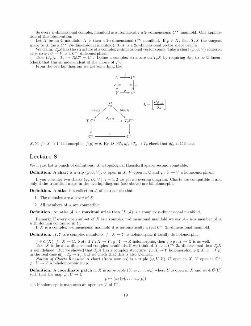
From the overlap diagram we get something like

f U �� U ′

ϕ ∼ ′ = = ϕ∼

g V �� V ′

� ∂ϕ1,2

� Tp

′ L =

����

���� ��������

∂z (dϕ1)p (dϕ2)p

�� dϕ1,2

T0Cn �� T0C

n

L Cn �� Cn

X,Y , f : X → Y holomorphic, f(p) = q. By 18.965, dfp : Tp → Tq check that dfp is C-linear.

Lecture 8

We’ll just list a bunch of definitions. X a topological Hausdorff space, second countable.

Definition. A chart is a trip (ϕ,U, V ), U open in X , V open in C and ϕ : U V a homeomorphism.→If you consider two charts (ϕi, Ui, Vi), i = 1, 2 we get an overlap diagram. Charts are compatible if and

only if the transition maps in the overlap diagram (see above) are biholomorphic.

Definition. A atlas is a collection A of charts such that

1. The domains are a cover of X

2. All members of A are compatible.

Definition. An atlas A is a maximal atlas then (X,A) is a complex n-dimensional manifold.

Remark: If every open subset of X is a complex n-dimensional manifold we say AU is a member of Awith domain contained in U .

If X is a complex n-dimensional manifold it is automatically a real C∞ 2n-dimensional manifold.

Definition. X,Y are complex manifolds, f : X Y is holomorphic if locally its holomorphic.→f : X C. Note if f : X Y , g : Y → Z holomorphic, then f ◦ g : X Z is as well.f ∈ O(X), → → →

Take X to be an n-dimensional complex manifolds, if we think of X as a C∞ 2n-dimensional then TpX is well defined. But we showed that TpX has a complex structure. f : X → Y holomorphic, p ∈ X , q = f(p) in the real case dfp : Tp → Tq, but we check that this is also C-linear.

Notion of Charts Revisited A chart (from now on) is a triple (ϕ,U, V ), U open in X , V open in Cn , ϕ : U V a biholomorphic map.→Definition. A coordinate patch in X is an n-tuple (U,w1, . . . , wn) where U is open in X and wi ∈ O(U) such that the map ϕ : U Cn →

p �→ (w1(p), . . . , wn(p))

is a biholomorphic map onto an open set V of Cn .

19

�

Charts and coordinate patches are equivalent.

Theorem (Implicit Function Theorem in Manifold Setting). Xn a manifold. U0 ⊆ X is an open set, f1, . . . , fk Assume df1, . . . , dfk are linearly independent at p. Then there exists a ∈ O(U0), p ∈ U0. coordinate patch (U,w1, . . . , wn), p ∈ U , U ⊂ U0 such that wi = fi for i = 1, . . . , k.

Proof. We can assume U0 is the domain of the chart (U0, V, ϕ), V an open set in Cn , ϕ : U0 V a biholomorphism. Then just apply last lecture version of implicity function theorem to fi ◦ (ϕ−1).

→

Submanifolds

X a complex n-dimensional manfiolds. Y ⊂ X a subset.

Definition. Y is a k-dimensional submanifold of X if for every p ∈ Y there exists a coordinate patch (U, z1, . . . , zn) with p ∈ U such that Y ∩ U is defined by the equation zk+1 = = zn = 0. · · ·

Remarks: A k dimensional submanifold of X is a k-dimensional complex manifold in its own right.Call a coordinate patch with the property above an adapted coordinated for X . The collection of

(n+ 1)-tuples (U ′ U ′ gives an atlas for X .|

By the implicit function theorem this definition is equivalent to the following weaker definition.

′ ), (U, z , . . . , z1k′ , . . . , z1 n), U

′ = U ∩ Y , z′ i, z = zi

Definition. Y is a k-dimensional submanifold X if for every p ∈ Y there exists an open set U of p in X and fi ∈ O(U) where i = 1, . . . , l, l = n− k such that df1, . . . , dfl are linearly independent at p and Y ∩ U , f1 = = fl = 0, i.e. locally Y is cut-out by l independent equation. · · ·

Examples

Affine non-singular algebraic varieties in Cn . These are X-dimensional submanifolds, Y of Cn such that for every p ∈ Y the fi’s figuring into the equation above (the ones that cut-out the manifold) are polynomials.

Projective counterparts We start by constructing the projective space CPn . Start with Cn+1 − {0}. Given 2 (n+ 1)-tuples we say

′ n)

= λzi, i = 0, . . . , n. [z0, z1, . . . , zn] are equivalence classes.

′ , . . . , z 1′ , z 0(z0, z1, . . . , zn) ∼ (z

in Cn − {0} if there exists λ ∈ C − {0} with zWe define CPn to be these equivalence classes Cn+1

′ i

.− {0}/ ∼We make this into a topological space by π : Cn+1 − {0} → CPn, which is given by

(z0, z1, . . . , zn) ∼ [z0, z1, . . . , zn]

We topologize CPn by giving it the weakest topology that makes π continuous, i.e. U ⊆ CPn is open if π−1(U) is open.

Lemma. With this topology CPn is compact.

Proof. Take 2 2

S2n+1 = {(z0, . . . , zn) z0 + · · · + zn = 1}|| | | |

and we note π(S2n+1) = CPn

so its the image of a compact set under a continuous map, so its compact.

Lemma. CPn is a complex n-manifold.

Proof. Define the standard atlas for CPn . For i = 0, . . . , n take

Ui = {[z0, . . . , zn] ∈ CPn , zi = 0}

Take Vi = Cn and define a map ϕi : Ui Vi by →

zi zn �

[z0, . . . , z

� z0 , . . . ,

�, . . . , n] �→

zi zi zi

20

��

�

�

�

�

ϕ−i

1 : Cn → Ui is given by (w1, . . . , wn) �→ [w1, . . . , 1, . . . , wn]

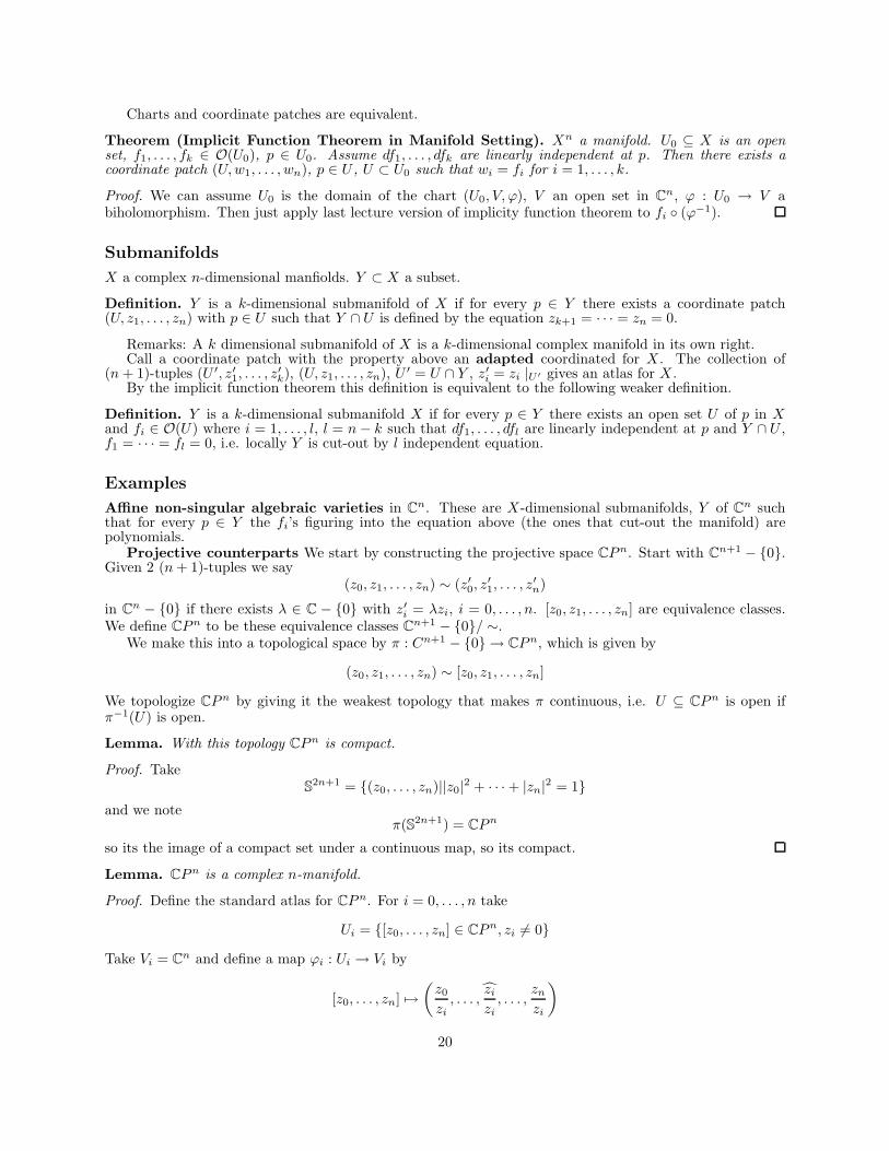
where w1 is in the 0th place, and 1 is in the ith place. The overlap diagrams for U0 and U1 are given by

U0 ∩ U1

ϕ0 ϕ1

����

����

� ���������ϕ0,1

���� V1,0V0,1

We can check that V0,1 = V1,0 = {(z1, . . . , zn), zi = 0}. Also check that �

1 z2 zn �

ϕ0,1 : V0,1 V1,0 (z1, . . . , z , , . . . ,→ n) �→ z1 z1 z1

This standard atlas gives a complex structure for CPn .

Lecture 9

We have a manifold CPn . Take αP (z0, . . . , P zn) =

� cαz

|α|=m

a homogenous polynomial. Then

1. P (λz) = λmP (z), so if P (z) = 0 then P (λz) = 0

2. Euler’s identity holds n

∂P� zi = mP ∂zii=0

Lemma. The following are equivalent

1. For all z ∈ Cn+1 − {0}, dPz = 0

2. For all z ∈ Cn+1 = 0, dPz = 0.− {0}, P (z) �

we call P non-singular if one of these holds.

If X = {[z0, . . . , zn], P (z) = 0}. Note that this is a well-defined property of homogeneous polynomials.

Theorem. If P is non-singular, X s an n− 1 dimensional submanifold of CPn .

Proof. Let U0, . . . , Un be the standard atlas for CPn . It is enough to check that X ∩ Ui is a submanifold ofUi. WE’ll check this for i = 0.

= Consider the map γCn ∼

U0 given by−→ γ(z1, . . . , zn) = [1, z1, . . . , zn]

It is enough to show that X0 = γ−1(X) is a complex n−1 dimensional submanifold of Cn . Let p(z1, . . . , zn) = P (1, z1, . . . , zn). X0 is the set of all points such that p = 0. It is enough to show that p(z) = 0 implies dpz = 0 (showed last time that this would then define a submanifold)

Suppose dp(z) = p(z) = 0. Then

∂Pp(1, z1, . . . , zn) = 0 = (1, z1, . . . , zn) = 0 i = 1, . . . , n

∂zi

By the Euler Identity

n∂P

0 = P (1, z1, . . . , zn) = �

zi (1, z1, . . . , zn) + � ∂P

(1, z1, . . . , zn)∂zi ∂zii=0

So ∂P (1, z1, . . . , zn) = 0, which is a contradiction because we assumed p = 0.∂zi

21

�

Theorem (Uniqueness of Analytic Continuation). X a connected complex manifold, V ⊆ X is an open set , f, g ∈ O(X). If f = g on V then f = g on all of X.

Sketch. Local version of UAC plus the following connectedness lemma

Lemma. For p, q ∈ X there exists open sets Ui, i = 1, . . . , n such that

1. Ui is biholomorphic to a connected open subset of Cn

2. p ∈ U1

3. q ∈ Un

4. Ui ∩ Ui+1 = ∅. Theorem. If X is a connected complex manifold and f ∈ O(X) then if for some p ∈ X, f : X R takes | | →a local maximum then f is constant.

Corollary. If X is compact and connected O(X) = C.

This implies that the Whitney embedding theorem does not hold for holomorphic manifolds. Let X be a complex n-dimensional manifold, X a real 2n dimensional manifold. Then if p ∈ X then TpX

is a real 2n-dimensional vector space and TpX is a complex n-dimensional vector space. Think for the moment of TpX as being a 2n-dimensional R-linear vector space. Define

Jp : TpX → TpX Jpv = √−1v

Jp is R-linear map with the property that Jp 2 = −I. We want to find the eigenvectors. First take Tp ⊗ C

and extend Jp to this by Jp(v ⊗ c) = Jpv ⊗ c

Now, Jp is C-linear, Jp : Tp ⊗ C → Tp ⊗ C. Also, we can introduce a complex conjugation operator

v ⊗ c: Tp ⊗ C v ⊗→ Tp ⊗ C c �→ We can split the tangent space by

Tp ⊗ C = T 1,0 ⊕ T 0,1 p p

where v ∈ T 1,0 if Jpv = +√−1v and v ∈ T 0,1 if Jpv = −

√−1v. i.e. we break Tp ⊗ C into eigenspaces. p p

If v ∈ T 1,0 iff v ∈ T 0,1 and so the dimension of the two parts of the tangent spaces are equal. p p

We can also take Tp∗ ⊗ C = (Tp

∗)1,0 ⊕ (Tp∗)0,1 and l ∈ (Tp

∗)1,0 if and only if J∗l = √−1l, l ∈ (Tp

∗)0,1 if

J∗l = −√−1l.

p

p

Check that l ∈ (Tp∗)1,0 if and only if l : Tp C is actually C-linear. To do this J∗l =

√−1l implies →

J∗l(v) = l(Jpv) = √−1l(v) which implies that l is C-linear. p

Corollary. U is open in X and p ∈ U . Then if f ∈ O(U then dfp ∈ (Tp∗)1,0 .

Corollary. (U, z1, . . . , zn) a coordinate patch then (dz1)p, . . . , (dzn)p is a basis of (Tp∗)1,0 and (dz1)p, . . . , (dzn)p

is a basis of (Tp∗)0,1 .

From the splitting above we get a splitting of the exterior product

Λk(Tp ∗ ⊗ C)

� Λl,m(Tp

∗ ⊗ C)= l+m=k

for ν1, . . . , νn a basis of T ∗ ⊗ C then p

ω ∈ Λl,m(T ∗ p ⊗ C) ⇔ ω =

� cI,J νI ∧ νJ

We also get a splitting in the tangent bundle

Λk (T ∗ ⊗ C) �

Λk,l(T ∗ ⊗ C)= l+m=k

22

since Ωk (X) is sections of Λk(T ∗ ⊗ C). Then

Ωk (X) = �

Λl,m(X) l+m=k

Locally when (U, z1, . . . , zn) is a coordinate patch, ω ∈ Ωl,m(U) iff

ω = �

aI,J dzI ∧ dzJ

so we’ve extended the Dolbeault complex to arbitrary manifolds.

Lecture 10

IF (U, z1, . . . , zn) is a coordinate patch, then this splitting agrees with our old splitting. Son on a complex manifold we have the bicomplex (Ω∗,∗, ∂, ∂). Again, we have lots of interesting subcomplexes.

�� Ωp,1Ap(X) = Ap = ker ∂ : Ωp,0

the complex of holomorphic p-forms on X , i.e. on a coordinate patch ω ∈ Ap(U)

ω = �

fI dzI fI ∈ O(U)

Now, for the complex Ap(X) we can compute its cohomology. There are two approaches to this

1. Hodge Theory

2. Sheaf Theory

We’ll talk about sheaves fora bit. Let X be a topological space. Top(X) is the category whose objects are open subsets of X and morphisms

are the inclusion maps.

Definition. A pre-sheaf of abelian groups is a contravariant functor F from Top(X) to the category of abelian groups.

In english: F attached to every open set U ⊂ X an abelian group F(U) and to every pair of open sets U ⊃ V a restriction map rU,V : F(U) → F(V ).

The functorality of this is that if U ⊃ V ⊃W then rU,W = rV,W · rU,V . Examples

1. The pre-sheaf C, U C(U) = the continuous function on U . Then the restrictions are given by→rU,V : C(U) → C(V ) V ∈ C(V )C(U) ∋ f �→ f |

2. X a C∞ manifold. The pre-sheaf of C∞ functions, U C∞(U). rU,V are as in 1.→3. Ωr is a pre-sheaf, U Ωr (U). Restriction is the usual restriction.→4. X a complex manifold, then Ωp,q, U Ωp,q(U) is a pre-sheave.→5. X a complex manifold, then you have the sheaf U → O(U).

Consider the pre-sheaf of C∞-functions. Let {Ui} be a collection of open set n X and U = � Ui. We claim

that C1 has the following “gluing property”: Given fi ∈ C∞(Ui) suppose

rUi,Ui∩Ujfi = rUj ,Ui∩Uj

fj

i.e. fi = fj on Ui ∩ Uj . Then there is a unique f ∈ C∞(U) such that

rU,Ui f = fi

Definition. A pre-sheaf F is a sheaf if it has the gluing property.

(Note that all of all pre-sheaves in the examples are sheaves)

23

�

Sheaf Cohomology

Let U = {Ui, i ∈ I}, I an index set, Ui an open cover of X . Let J = (j0, . . . , jk ) ∈ Ik+1 , then define

UJ = Uj0 ∩ · · · ∩ Ujk

Take Nk ⊆ Ik+1 and let us say that J ⊂ Nk if and only if UJ = ∅ and take

N = � Nk

then this is a graded set called the nerve of the cover Ui. Nk is called the k-skeleton of N .

Let F be the sheaf of abelian groups in X

Definition. A Cech cochain, c of degree k, with values in F is a map that assigns to every J ∈ Nk an element c(J) ∈ F(UJ ).

Notation. J ∈ Nk , J = (j0, . . . , jk ) and ji ∈ I for all 0 ≤ i ≤ k. Then define

Ji = (j0, . . . , j�i, . . . , jk )

then Ji ∈ Nk−1 and let ri = rUJi ,UJ

.

We can define an coboundary operator

δ : Ck−1(U,F) → Ck (U,F)

For J ∈ Nk and c ∈ Ck−1 define δc(J) =

�(−1)i ric(Ji)

i

(note that this makes sense, because c(Ji) ∈ F(UJi ).

Lemma. δ2 = 0, i.e. δ is in fact a coboundary operator.

Proof. J ∈ Nk+1 then

(δδc)(J) = �

(−1)i riδc(Ji) i

= �

(−1)i rirj �

(−1)j c(Ji,j )+ i j<i �(−1)i rirj

�(−1)j−1 c(Ji,j )

i j>i

this is symmetric in i and j, so its 0.

Because δ is a coboundary operator we can consider Hk(U ,F), the cohomology groups of this complex. What is H0(U,F)? Consider c ∈ C0(U,F) then every i ∈ I, c(i) = fi ∈ F(Ui). If δc = 0 then rifj = rj fi

for all i, j. Then the gluing property of F tells us that there exists an f ∈ F(X) with rif = fi, so we have proved that H0(X,F) = F(X), the global sections of the sheaf.

For today, we’ll just compute Hk(U,C∞) = 0 for all k ≥ 1. The proof is a bit sketchy. Let {ρr }r∈I be a partition of unity subordinate to {Ui, i ∈ I}. Then ρr ∈ C0

∞(Ur) and � ρr = 1 by

definition. Given J ∈ Nk−1 let (r, J) = (r, j0, . . . , jk−1) and define a coboundary operator

Q : Ck (U,F) → Ck−1(U,F)

Take c ∈ Ck , J ∈ Nk−1 then

Qc(J) = �

ρrc(r, J) ∈ C∞(UJ )

24

� � . . .

� � . . .

Explanation: First notice that (r, J) may not be in Nk . But in this case Ur and UJ are disjoint, so ρr ≡ 0 on UJ , so we just make these terms 0. What if (r, J) ∈ Nk then c(r, J) ∈ C∞(Ur ∩UJ ) (but we want Qc(J) to be C∞(UJ ).

But �ρr c(r, J) on Ur ∩ UJρr c(r, J) = 0 on UJ − (Ur ∩ UJ )

and ρr ∈ C∞(Ur ).

Proposition. δQ + Qδ = id.

Corollary. Hk (U,C∞) = 0.

The same argument works for the sheaves Ω∗, Ωp,q , but NOT however for O.

Lecture 11

U open in Cn , ρ ∈ C∞(U), ρ : U → R ten ρ is strictly plurisubharmonic if for all p ∈ U the matrix

� ∂2ρ

�

(p)∂zi∂zj

is positive definite. If U, V open in Cn then ϕ : U → V is biholomorphic then for ρ ∈ C∞(V ) strictly plurisubharmonic ϕ∗ρ

is also strictly plurisubharmonic. If q = ϕ(p)

∂2 ∂2ρ ∂ϕk ∂ϕlϕ∗ρ(q) =

�

∂zizj ∂zi∂zl ∂zl ∂zjk,l

the RHS being s.p.s.h implies the right hand side is also.

Definition. U open in Cn is pseudo-convex if it admits a s.p.s.h exhaustion function. We discussed the examples before (in particular if U1, U2 pseudo-convex, U1 ∩ U2 is pseudo-convex)

The observation above gives that pseudoconvexity is invariant under biholomorphism.

Theorem (Hormander). U pseudo-convex then the Dolbeault complex on U is exact.

Back to Cech Cohomology

X a complex n-dimensional manifold and U = {Ui, i ∈ I} and F a sheaf of abelian groups. We get the Cech complex

C0(U ,F) δ �� C1(U ,F)

δ

and Hp(U ,F) is the cohomology group of the Cech complex. We proved earlier that H0(U ,F) = F(X). ,Ωp,qAlso, we showed that if F is one of the sheaves that we discussed Hp(U ,F) = 0, p > 0 i.e. F = C∞, Ωr .

But what we’re really interested in is F = O.

Definition. U = {Ui, i ∈ I} is a pseudoconvex cover if for each i, Ui is biholomorphic to a pseudoconvex open set of Cn .

Theorem. If U is a pseudoconvex cover then the Cech cohomology groups Hp(U ,O) are identified with the cohomology groups of the Dolbeault complex

Ω0,0(X) ∂ �� Ω0,1(X)

∂ ��∂ �� Ω0,2(X) ∂

25

� � � �

� � . . .

� � . . .

� � � � � � � �

� � � � � � � �

� � � � � � � �

� � � � � � � �

� � � � � � � �

This is pretty nice, because its a comparison of very different objects. We do a proof by diagram chasing. The rows of this diagram are

δ 0

δ �� Ω0,q(X) δ �� C0(U ,Ω0,q ) �� C1(U ,Ω0,q)

δ �� . . .

To figure out the columns we have to create another way looking at the Cech complex. Let N be the nerve of U , J ∈ Np, c ∈ Cp(U ,Ω0,q ) iff c assigns to J an element c(J) ∈ Ω0,q (UJ ).

Define ∂c ∈ Cp(U ,Ω0,q+1) by

∂c(J) = ∂(c(J))

now ∂ : Cp(U ,Ω0,q ) → Cp(U ,Ω0,q+1) and we can show that ∂ 2

= 0. Its not hard to show that the diagram below commutes.

Cp(U ,Ω0,q ) δ �� Cp+1(U ,Ω0,q )

∂ ∂

Cp(U ,Ω0,q+1) δ �� Cp+1(U ,Ω0,q+1)

Consider the map Cp(U ,Ω0,0) ∂ Cp(U ,Ω0,1), what is the kernel of ∂. c ∈ Cp(U ,Ω0,0), J ∈ Np, c(J) ∈−→

C∞(UJ ) and ∂c(J) = 0 then c(J) ∈ O(UJ ). So we can extend the arrow that we are considering as follows

Cp(U ,O) i �� Cp(U ,Ω0,0)

∂ �� Cp(U ,Ω0,1)

Theorem. The following sequence is exact

Cp(U ,Ω0,0) ∂ �� Cp(U ,Ω0,1)

∂

Observation: J ∈ Np. The set UJ is biholomorphic to a pseudoconvex open set in Cn . Why? UJ is non-empty and it is the intersection of pseudoconvex sets, and so it is also pseudoconvex.

Suppose we have c ∈ Cp(U ,Ω0,q ) and ∂c = 0. For J ∈ Np, c(J) ∈ C∞(UJ ) and ∂c(J) = 0. So there is

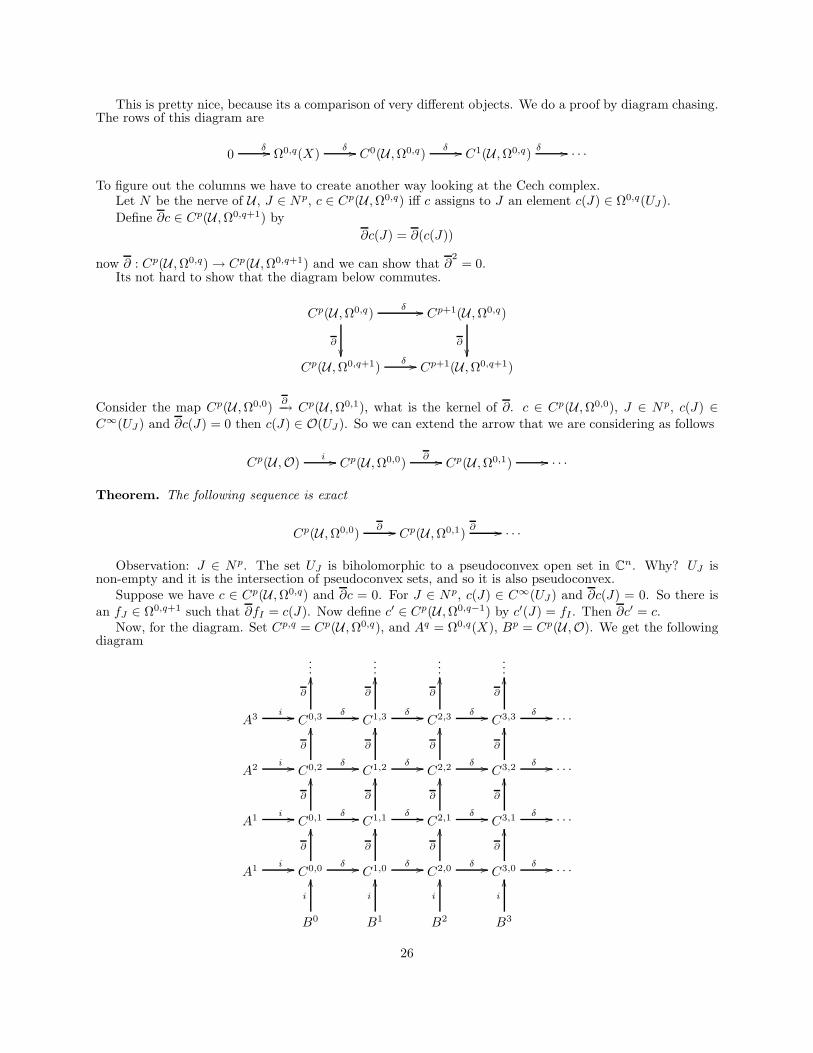
an fJ ∈ Ω0,q+1 such that ∂fI = c(J). Now define c ′ ∈ Cp(U ,Ω0,q−1) by c ′(J) = fI . Then ∂c ′ = c. Now, for the diagram. Set Cp,q = Cp(U ,Ω0,q ), and Aq = Ω0,q (X), Bp = Cp(U ,O). We get the following

diagram

. . . . . . . . . . . .

∂ ∂ ∂ ∂

i δ δ δ δ�� C0,3 �� C1,3 �� C2,3 �� C3,3 �� . . .A3

∂ ∂ ∂ ∂

i δ δ δ δ A2 �� C0,2 �� C1,2 �� C2,2 �� C3,2 �� . . .

∂ ∂ ∂ ∂

i δ δ δ δ�� C0,1 �� C1,1 �� C2,1 �� C3,1 �� . . .A1

∂ ∂ ∂ ∂

i δ δ δ δ�� C0,0 �� C1,0 �� C2,0 �� C3,0 �� . . .A1

i i i i

B0 B1 B2 B3

26

All rows except the bottom row are exact, all columns except the the left are exact. The bottom row computes Hp(U , O) and the left hand column computes Hq(X, Dolbeault). We need to prove that the cohomology of the bottom row is the cohomology of the left.

Hint: Take [a] ∈ Hk (X, Dolbeault), a ∈ Ak = Ω0,k (X). The we just diagram chase down and to the right, eventually we get down to a [b] ∈ Hk (U , O). We have to prove that this case [a] [b] is in fact a mapping (we do this by showing that the chasing does not change cohomology class) and we have to show that the map created is bijective, which is not too hard.

27

Chapter 3

Symplectic and Kaehler Geometry

Lecture 12

Today: Symplectic geometry and Kaehler geometry, the linear aspects anyway.

Symplectic Geometry

Let V be an n dimensional vector space over R, B : V × V R a bilineare form on V .→ Definition. B is alternating if B(v, w) = −B(w, v). Denote by Alt2(V ) the space of all alternating bilinear forms on V .

Definition. Take any B ∈ Alt(V ), U a subspace of V . Then we can define the orthogonal complement by

U⊥ = {v ∈ V,B(u, v) = 0, ∀u ∈ U}

Definition. B is non-degenerate if V ⊥ = {0}. Theorem. If B is non-degenerate then dim V is even. Moeover, there exists a basis e1, . . . , en, f1, . . . , fn of V such that B(ei, en) = B(fi, fj ) = 0 and B(ei, fj ) = δij

Definition. B is non-degenerate if and only if the pair (V,B) is a symplectic vector space. Then ei’s and fj ’s are called a Darboux basis of V .

Let B be non-degenerate and U a vector subspace of V Remark: dim U⊥ = 2n− dim V and we have the following 3 scenarios.

1. U isotropic ⇔ U⊥ ⊃ U . This implies that dim U ≤ n

2. U Lagrangian ⇔ U⊥ = U . This implies dim U = n.

3. U symplectic ⇔ U⊥∩U = ∅. This implies that U⊥ is symplectic and B U and B U ⊥ are non-degenerate. | |Let V = V m be a vector space over R we have

Alt2(V ) ∼= Λ2(V ∗)

is a canonical identification. Let v1, . . . , vm be a basis of v, then

Alt21 �

B(vi, vj )vi ∗ ∧ vj∗(V ) ∋ B �→

2

and the inverse Λ2(V ∗) ∋ ω �→ Bω ∈ Alt2(V ) is given by

B(v, w) = iW (iV ω)

Suppose m = 2n.

29

�Theorem. B ∈ Alt2(V ) is non-degenerate if ωB ∈ Λ2(V ) satisfies ωn = 0B

1/2 of Proof. B non-degenerate, let e1, . . . , fn be a Darboux basis of V then

ωB = �

ei ∗ ∧ fj∗

and we can show ωn = n!e∗ = 0B 1 ∧ f∗

n ∧ f∗ n1 ∧ · · · ∧ e∗ �

Notation. ω ∈ Λ2(V ∗), symplectic geometers just say “Bω (v, w) = ω(v, w)”.

Kaehler spaces

V = V 2n , V a vector space over R, B ∈ Alt2(V ) is non-generate. Assume we have another piece of structure a map J : V → V that is R-linear and J2 = −I. Definition. B and J are compatible if B(v, w) = B(Jv, Jw).

Exercise(not to be handed in) Let Q(v, w) = B(v, Jw) show that B and J are compatible if and only if Q is symmetric.

From J we can make V a vector space over C by setting √−1v = Jv. So this gives V a structure of

complex n-dimensional vector space.

Definition. Take the bilinear form H : V × V C by →1

H(v, w) = √−1(B(v, w) +

√−1Q(v, w))

B and J are compatible if and only if H is hermitian on the complex vector space V . Note that H(v, v) = Q(v, v).

Definition. V, J,B is Kahler if either H is positive definite or Q is positive definite (these two are equivalent).

Consider V ∗ ⊗ C = HomR(V,C), so if l ∈ V ∗ ⊗ C then l : V C.→

Definition. l ∈ (V ∗)1,0 if it is C-linear, i.e. l(Jv) = √−1l(v). And l ∈ (V ∗)0,1 if it is C-antilinear, i.e.

l(Jv) = −√−1l(v).

¯Definition. lv = l(v). J∗l(v) = lJ(v).

¯Then if l ∈ (V ∗)1,0 then l ∈ (V ∗)0,1 . If l ∈ (V ∗)1,0 then J∗l = √−1l, l ∈ (V ∗)0,1 , J∗l = −

√−1l.

So we can decompose V ∗ ⊗ C = (V ∗)1,0 ⊕ (V ∗)0,1 i.e. decomposing into ±√−1 eigenspace of J∗ and

(V ∗)0,1 = (V ∗)0,1 . This decomposition gives a decomposition of the exterior algebra, Λr(V ∗ ⊗ C) = Λr (V ∗) ⊗ C. Now, this

decomposes into bigraded pieces

Λr (V ∗ ⊗ C) �

Λk,l(V ∗)= k+l=r

Λk,l(V ∗) is the linear span of k, l forms of the form

νl µiνj ∈ (V ∗)1,0 µ1 ∧ · · · ∧ µk ∧ ν1 ∧ · · · ∧ ¯

Note that J∗ : V ∗ ⊗ C → V ∗ ⊗ C can be extended to a map J∗ : Λr (V ∗ Λr(V ∗ ⊗ C) by setting ⊗ C) →=J∗(l1 ∧ · · · ∧ lr ) J∗l1 ∧ · · · ∧ J∗lr

on decomposable elements l1 ∧ · · · ∧ lr ∈ Λr . We can define complex conjugation on Λr (V ∗ ⊗ C) on decomposable elements ω = by ¯ ¯

l1 ∧ · · · ∧ lr

ω = lr. Λr(V ∗ ⊗C) = Λr(V )⊗C, then ¯ ω ∈ Λl,k(V ∗) l1 ∧ · · · ∧

ω = ω if and only if ω ∈ Λr(V ∗) . And if ω ∈ Λk,l(V ∗) then ¯

30

�

Proposition. On Λk,l(V ∗) we have J∗ = (√−1)k−l Id.

Proof. Take ω = νl, µi, νi ∈ (V ∗)1,0 then µ1 ∧ · · · ∧ µk ∧ ν1 ∧ · · · ∧ ¯

J∗ω = J∗µ1 ∧ · · · ∧ J∗µk ∧ J∗ν1 ∧ · · · ∧ J∗νl = (−1)k (−√−1)lω

Notice that for the following decomposition of Λ2(V ⊗ C) the eigenvalues of J∗ are given below

Λ2(V ⊗ C) = Λ2,0 ⊕Λ1,1 ⊕Λ0,2

� �� � ���� ���� ���� 1 −1 −1J∗

So if ω ∈ Λ∗(V ∗ ⊗ C) then if Jω = ω. Now, back to serious Kahler stuff. Let V,B, J be Kahler. B �→ ωB ∈ Λ2(V ∗) ⊂ Λ2(V ∗) ⊗ C.B is J invariant, so ωB is J-invariant, which happens if and only if ωB ∈ Λ1,1(V ∗) and ωB is real if and

¯only if ωB = ωB . So there is a -1 correspondence between J invariant elements of Λ2(V ) and elements ω ∈ Λ1,1(V ∗) which

are real. Observe: (V ∗)1,0 ⊗ V ∗)0,1

ρ Let µ1, . . . , µn be a basis of (V ∗)1,0 . Take −→ Λ1,1(V ∗) by µ⊗ ν �→ µ ∧ ν.

µj ∈ (V ∗)1,0 ⊗ (V ∗)0,1α = �

aij µi ⊗ ¯

Take ρ(α) =

� aij µi ∧ µj

1is it true that ρ(α) = ρ(α). No, not always. This happens if aij = −aij , equivalently √−1[aij ] is Hermitian.

We have Alt2 = ωB ∈ Λ1,1(V ∗)(V ) ∋ B �→ ω

1Take α = ρ−1(ω), H = √−1 α. Then H is Hermitian.

1Check that H = √−1(B +

√−1Q), B Kahler iff and only if H is positive definite.

Lecture 13

X2n a real C∞ manifold. Have ω ∈ Ω2(X), with ω closed.

=For p ∈ X we saw last time that Λ2(Tp∗) ∼ Alt2(Tp), so ωp ↔ Bp.

Definition. ω is symplectic if for every point p, Bp is non-degenerate.

Remark: Alternatively ω is symplectic if and only if ωn is a volume form. i.e. ωn = 0 for all p.p

Theorem (Darboux Theorem). If ω is symplectic then for every p ∈ X there exists a coordinate patch (U, x1, . . . , xn, y1, . . . , yn) centered at p such that on U

ω = �

dxi ∧ dyi

(in Anna Cannas notes)

Suppose X2n is a complex n-dimensional manifold. Then for p ∈ X , TpX is a complex n-dimensional

vector space. So there exists an R-linear map Jp : Tp → Tp, Jpv = √−1v with J2 = −I.p

Definition. ω symplectic is Kahler if for every p ∈ X , Bp and Jp are compatible and the quadratic form

Qp(v, w) = Bp(v, Jpw)

is positive definite.

31

This Qp is a positive definite symmetric bilinear form on Tp for all p, so X is a Riemannian manifold as well.

We saw earlier that Jp and Bp are compatible is equivalent to the assumption that ω ∈ Λ1,1(Tp∗).

Last time we say there was a mapping

= ρ : (T ∗)1,0 ⊗ (T ∗)0,1

∼Λ1,1(Tp

∗) Hp ↔ ωp−→ The condition ωp = ωp tells us that Hp is a hermitian bilinear form on Tp. The condition that Qp is positive definite implies that Hp is positive definite.

Let (U, z1, . . . , zn) be a coordinate patch on X

ω = √−1�

hij dzi ∧ dzj hi,j ∈ C∞(U)

so Hp =

� hij (p)(dzi)p ⊗ (dzj )p

the condition that Hp ≫ 0 (≫ means positive definite) implies that hij (p) ≫ 0. What about the Riemannian structure? The Riemannian arc-length on U is given by

ds 2 = �

hij dzidzj

Darboux Theorem for Kahler Manifolds

Let (U, z1, . . . , zn) be a coordinate patch on X , let U be biholomorphic to a polydisk z1 < ǫ1, . . . , zn < ǫn.| | | |Let ω ∈ Ω1,1(U), dω = 0 be a Kaehler form. dω = 0 implies that ∂ω = ∂ω = 0, which implies (by a theorem we proved earlier) that for some F

ω = √−1∂∂F F ∈ C∞(U)

(it followed from the exactness of the Dolbeault complex). Also, since ω = ω we get that

ω = ω = −√−1∂∂F =

√−1∂∂F

So replacing F by 1 2 (F + F ) we can assume that F is real-valued. Moreover

∂2F ω =

√−1∂∂F =

√−1�

dzi ∧ dzj∂zi∂zj

so we conclude that ∂2F

(p) ≫ 0 ∂zi∂zj

for all p ∈ U , i.e. F ∈ C∞(U)is a strictly plurisubharmonic function. So we’ve proved

Theorem (Darboux). If ω is a Kahler form then for every poiont p ∈ X there exists a coordinate patch

(U, z1, . . . , zn) cenetered at p and a strictly plurisubharmonic function F on U such that on U , ω = √−1∂∂F .

All of the local structure is locally encoded in F , the symplectic form, the Kahler form etc.

Definition. F is called the potential function

This function is not unique, but how not-unique is it? Let U be a simply connected open subset of X and let F1, F2 ∈ C∞(U) be potential functions for the

Kahler metric. Let G = F1 − F2. If ∂∂F1 = ∂∂F2 then ∂∂G = 0. Now, ∂∂G = 0 implies that d∂G = 0, so ∂G is a closed 1-form. U simply connected implies that there exists an H ∈ C∞(U) so that ∂G = dH , so

∂G = ∂H , and ∂H = 0. Let K1 = G − H , K2 = Ten G = K1 + K2. But G is real-valued, so G = G so H , K1, K2 ∈ O.

K1 + K2 = K1 + K2 which implies K1 −K2 = K1 −K2 so K1 −K2 is a real-valued holomorphic function on U . But real valued and holomorphic implies that the function is constant. Thus K1 −K2 is a constant. Adjusting this constant we get that K1 = K2.

Let K = K1 = K2, then G = K + K.

32

Theorem. If F1 and F2 are potential functions for the Kahler metric ω on U thenm F1 = F2 + (K + K) where K ∈ O(U).

Definition. Let X be a complex manifold, U any open subset of X . F ∈ C∞(U), F is strictly plurisubhar­monic if

√−1∂∂F = ω is a Kahler form on U . This is the coordinate free definition of s.p.s.h

Definition. An open set U of X is pseudoconvex if it admits a s.p.s.h. exhaustion function.

Remarks: U is pseudoconvex if the Dolbeault complex is exact.

Definition. X is a stein manifold if it is pseudoconvex

Examples of Kaehler Manifolds

21. Cn . Let F = z 2 = z1 + + zn2 and then | | | | · · · | |

√−1∂∂f =

√−1�

dzi ∧ dzj = ω

and if we say zi = xi + √−1y then

ω = 2�

dxi ∧ dyi then standard Darboux form.

2. Stein manifolds.

3. Complex submanifolds of Kaehler manifolds. We claim that if Xn is a complex manifold, Y k a complex submanifold in X if ι : Y X is an inclusion. Then →(a) If ω is a Kaehler form on X , ι∗ω is a Kaehler form.

(b) If U is an open subset of X and F ∈ C∞(U) is a potential function for ω on U the ι∗F is a potential function for the form ι∗ω on U ∩ Y .

b) implies a), so it suffices to prove b). Let (U, z1, . . . , zn) be a coordinate chart adapted for Y , i.e

Y ∩ U is defined by zk+1 = = zn = 0. ω = √−1∂∂F on U , so since ι is holomorphic it commutes · · ·

with ∂, ∂. Then ι∗ω =

√−1∂∂ι∗F ι∗F = F (z1, . . . , zk , 0, . . . , 0)

To see this is Kaehler we need only check that ι∗F is s.p.s.h. Take p ∈ U ∩ Y . We consider the matrix

� ∂2F

�

(p) 1 ≤ i, j ≤ k ∂zi∂zj

But this is the principle k × k minor of

� ∂2F

�

(p) 1 ≤ i, j ≤ n ∂zi∂zj

and the last matrix is positive definite, by definition (and since its a hermitian matrix its principle k × k minors are positive definite)

4. All non-singular affine algebraic varieties.

Lecture 14

2 2We discussed the Kaehler metric corresponding to the potential function F (z) = z 2 = z1| + · · · + zn .| |Another interesting case is to take the potential function F = Log |z|2 on Cn+1

| |. This is not s.p.s.h.

|

But recall we have a mapping − {0}

Cn+1 π

CPn π(z0, . . . , zn) = [z0, . . . , zn]− {0} −→

33

2Theorem. There exists a unique Kaehler form ω on CP b such that π∗ω = √−1∂∂ Log z . This is called

the Fubini-Study symplectic form. | |

We’ll prove this over the next few paragraphs. Let Ui = {[z0, . . . , zn], zi = 0} and let Oi = π−1(Ui) = {(z0, . . . , zn), zi = Define γi : Ui Oi by mapping γi([z0, . . . , zn]) =

�(z0, . . . , zn)/zi. Notice that →

π γi = idUi and

�γi

0}. π(z0, . . . , zn) = (z0, . . . , zn)/zi.◦ ◦

Lemma. Let µ = √−1∂∂ Log |z|2 on Cn+1 Then on Oi we have π∗γi

∗µ = µ.− {0}. Proof.

2 �

22π∗γ∗ Log |z|2 = (γiπ)∗ Log |z| = Log

�

||z

z

i

||2 = Log z 2 − Log zii | | | |

2 2π∗γi ∗µ =

√−1π∗γi

∗∂∂ Log z = √−1∂∂(Log z − Log |zi|2)

2

| | | |2 =

√−1∂∂(Log z − Log zi − Log zj ) =

√−1∂∂ Log z = µ| | | |

Corollary. We have local existence and uniqueness of ω on each Ui, which implies global existence and uniqueness.

So we know there exists ω on CPn such that π∗ω = √−1∂∂ Log z 2 . We want to show that Kaehlerity | |

of ω. Define ρi : C

n Oi ρi(z1, . . . , zn) = (z1, . . . , 1, . . . , zn)→ Then π ρi : C

n Ui is a biholomorphism. It suffices to check that ◦ → 2(π ρi)

∗ω = ρ∗ i π∗ω = ρ∗µ = ρ∗ i (

√−1∂∂ Log z )◦

2 2 2= √−1∂∂ Log(1 + zi + + zn ) =

√−|1∂

| ∂ Log(1 + z )| | · · · | | | |

We must check that Log(1 + |z|2) is s.p.s.h.

∂ Log(1 + |z|2) =

1 +

zj |z|2∂zj

zizj 1∂ ∂∂zj Log(1 + |z|2) =

1 +

δij |z|2 − (1 + z 2)2

=1 + z 2

((1 + |z|2δij − zj zi)∂zi | | | |

We have to check that the term in parentheses is positive, but thats not too hard.

Corollary. All complex submanifolds of CPn are Kaehler.

Suppose we have (X,ω) a Kaehler manifold. We can associate to ω ∈ Ω1,1(X) another closed 2-form µ ∈ Ω1,1(X) called the Ricci form

Let (U, z1, . . . , zn) be a coordinate patch. Let F ∈ C∞(U) be a potential function for ω on U , i.e. ω =

√−1∂∂F . Let �

∂F �

G = det ∂zi∂zj

This is real and positive, so the log is well defined. Define

µ = √−1∂∂ LogG

Lemma. µ is intrinsically defined, i.e. it is independent of F and the coordinate system

Proof. Independent of F Take F1, F2 to be potential functions of ω on U . Then ∂∂F1 = ∂∂F2, which, in coordinates means that �

∂F1

� � ∂F2

�

= ∂zi∂zj ∂zi∂zj

34

= �

�

�

�

Independent of Coordinates On U ∩ U ′ the formula’s look like

∂F ∂2F ∂z′ k ∂zl ′ k ∂z

′ l ∂zi ∂z∂zi∂zj ∂z ′

jk,l

or in matrix notation � ∂F

� � ∂z

� � ∂2F

� � ∂z′ l

′ k = · ·′

k ∂z′ l∂zi∂zj ∂zi ∂z ∂zj

taking determinants we get � ∂F

� � ∂2F

� ¯det = HH ′

k ∂z′ l∂zi∂zj ∂z

where � z

H = det ′ k

zl so �

∂F � �

∂2F �

HLog det = Log det + Log det H + Log det ′ i∂z

′ j∂zi∂zj ∂z

LogH ∈ O(U) (at least on a branch). Apply ∂∂ to both sides of the above. That finishes it.

Definition. X, ω a Kaehler manifold and µ is the Ricci form. Then X is called Kaehler-Einstein if there exists a constant such that µ = λω.

Take µ = λω, λ = 0. Let (U, z1, . . . , zn) be a coordinate patch. For F ∈ C∞(U) a potential function for ω on U

µ = √−1∂∂ Log det

� ∂2F

�

= λω = λ√−1∂∂F

∂zi∂zj

By a theorem we proved last time �

∂2F �

Log det = λF = G + G ∂zi∂zj

G ∈ O(U)

Take F and replace it by 1

F F + (G + G)λ

then � ∂2F

� � ∂2F

�

Log det = λF det = e λF

∂zi∂zj ∂zi∂zj

The boxed formula is the Monge-Ampere equation. This is essential an equation for constructing Einstein-Kahler metrics.

Exercise Check that the Fubini-Study potential is Kaehler-Einstein with λ = −(n+1). F = Log(1+ z 2)| |locally on each Ui. So we need to check that F = Log(1 + z 2) satisfies the Monge-Ampere equations.| |

Lecture 15

Homework problem number 2. X a complex manifold. We know we have the splitting

Ωr (X) = �

Ωp,q(X) d = ∂ + ∂ p+q

¯ ∂We get the Dolbeault complex Ω0,0(X)

∂ Ω0,1(X) . . . and for every p we get a generalized Dolbeault→ −

complex − →

Ωp,0(X) ∂ �� Ωp,1(X)

∂ �� Ωp,2(X) ∂ �� . . .

35

this is the p-Dolbeault complex. Take ker ∂ : Ω0,0(X) → Ω0,1(X) this is O(X) and in general ker ∂ : Ωp,0(X) → Ωp,1(X). Call this Ap(X). For µ ∈ Ap(X) pick a coordinate patch (U, z1, . . . , zn) then

µ = �

fI (z)dzi1 ∧ · · · ∧ dzip

and ∂µ = 0 implies that ∂fI = 0, so fI ∈ O(U). These Ap are called the holomorphic de Rham complex. More general, take U open in X . Then Ap(X) defines a sheaf Ap on X . Exercise Let U = {Ui, i ∈ I} be a cover of X by pseudoconvex open sets. Show that the Cech cohomology

group Hq (U,Ap) coincide with the cohomology groups of

Ωp,0(X) ∂ �� Ωp,1(X)

∂ �� Ωp,2(X) ∂ �� . . .

We did the special case p = 0, i.e. we showed Hq (U,O) ∼ the Dolbeault complex.= The idea is to reduce this to the following exercise in diagram chasing. Let C =

� Ci,j be a bigraded

Ci,j+1vector space with commuting coboundary operators δ : Ci,j Ci+1,j and d : Ci,j .→ →C1,iLet Vi = ker di : C

i,0 → Ci,1 . Note that since dδ = δd that δVi ⊂ Vi+1. Also let W = ker δi : C0,i

and dWi ⊂Wi+1. →

Theorem. Suppose that the sequence

δ δ δ C0,i �� C1,i �� C2,i �� . . .

and the sequence d d d

Ci,0 �� Ci,1 �� Ci,2 �� . . .

are exact for all i. Prove that the cohomology groups of

δ δ δ�� V0 �� V1

�� V27 �� . . .0

and d d d�� W0

�� W1 �� W2

�� . . .0

are isomorphic.

36

Chapter 4

Elliptic Operators

This chapter by Victor Guillemin

4.1 Differential operators on Rn

Let U be an open subset of Rn and let Dk be the differential operator,

1 ∂ .

∂xk√−1

For every multi-index, α = α1, . . . , αn, we define

DαnDα = Dα1 .1 n· · ·

A differential operator of order r: P : C∞(U) → C∞(U) ,

is an operator of the form

Pu = �

aαDα u , .aα ∈ C∞(U)

α ≤r| |

Here α = α1 + αn.| | · · ·The symbol of P is roughly speaking its “rth order part”. More explicitly it is the function on U × R

n

defined by

(x, ξ) → �

aα(x)ξα =: p(x, ξ) . |α|=r

The following property of symbols will be used to define the notion of “symbol” for differential operators on manifolds. Let f : U → R be a C∞ function.

Theorem. The operator e−itf Pe itf uu ∈ C∞(U) →

is a sum r� tr−iPiu (4.1.1)

i=0

Pi being a differential operator of order i which doesn’t depend on t. Moreover, P0 is multiplication by the function

p0(x) =: P (x, ξ)

∂f with ξi = ∂xi , i = 1, . . . n.

37

Lecture 16

� � �

� �

� �

� � � �

Proof. It suffices to check this for the operators Dα . Consider first Dk :

e−itf Dke itf ∂f u = Dk u + t .

∂xk

Next consider Dα

e−itf Dα itf e−itf (Dα1 itf e u = Dαn )e u1 n· · ·= (e−itf D1e itf )α1 itf )αn · · · (e−itf Dne u

which is by the above ∂f �α1 ∂f �αn

�D1 + t

�Dn + t

∂x1 · · ·

2xn

and is clearly of the form (4.1.1). Moreover the tr term of this operator is just multiplication by

∂f�α1 ∂ �αn

� � . (4.1.2)

∂x1 · · ·

∂xn

Corollary. If P and Q are differential operators and p(x, ξ) and q(x, ξ) their symbols, the symbol of PQ is p(x, ξ) q(x, s).

Proof. Suppose P is of the order r and Q of the order s. Then

e−itf PQe itf �e−itf Pe itf

��e−itf Qe itf

�uu =

r s = �p(x, df)t +

��q(x, df)t +

�u· · · · · ·

r+s = �p(x, df)q(x, df)t +

�u . · · ·

Given a differential operator

P = �

aαDα

α ≤r| |

we define its transpose to be the operator

u ∈ C∞(U) → �

Dα aαu =: P t u . α ≤r| |

Theorem. For u, v ∈ C∞0 (U)

�Pu, v� =: Puv dx = u, P t .

Proof. By integration by parts �

1 �

∂ Dk u, v = Dkuv dx = uv dk � � √

−1 ∂xk

1 �

∂ �

= u v dx = uDkv dx −√−1 ∂xk

= u, dk v .

Thus

�Dα u, v = �u, Dα v

and

�aαDα u, v = �Dα u, aαv = u, Dα aαv , .

38

Exercises.

If p(x, ξ) is the symbol of P , p(x, ξ) is the symbol of pt .

Ellipticity.

P is elliptic if p(x, ξ) /∈ 0 for all x ∈ U and ξ ∈ Rn − 0.

4.2 Differential operators on manifolds.

Let U and V be open subsets of Rn and ϕ : U V a diffeomorphism. →Claim. If P is a differential operator of order m on U the operator

)∗Pϕ∗uu ∈ C∞(V ) → (ϕ−1

is a differential operator of order m on V .

Proof. (ϕ−1)∗Dαϕ∗ = �(ϕ−1)∗D1ϕ

∗�α1 �(α−1)∗Dnϕ

∗�αn so it suffices to check this for Dk and for Dk· · ·

this follows from the chain rule

Dkϕ∗f =

� ∂ϕi ϕ∗Dif .

∂xk

This invariance under coordinate changes means we can define differential operators on manifolds.

Definition. Let X = Xn be a real C∞ manifold. An operator, P : C∞(X) → C∞(X), is an mth order differential operator if, for every coordinate patch, (U, x1, . . . , xn) the restriction map

Pu1Uu ∈ C∞(X) →

is given by an mth order differential operator, i.e., restricted to U ,

Pu = �

aαDα u , .aα ∈ C∞(U)

α ≤m| |

Remark. Note that this is a non-vacuous definition. More explicitly let (U, x1, . . . , xn) and (U ′, x1′ , . . . , xn

′ ) be coordinate patches. Then the map

u → Pu1U ∩ U ′

is a differential operator of order m in the x-coordinates if and only if it’s a differential operator in the x′-coordinates.

The symbol of a differential operator

Theorem. Let f : X → R be C∞ function. Then the operator

e−itf Pe−itf uu ∈ C∞(X) →can be written as a sum

m� tm−iPi

i=0

Pi being a differential operator of order i which doesn’t depend on t.

Proof. We have to check that for every coordinate patch (U, x1, . . . , xn) the operator

e−itf Pe itf 1Uu ∈ C∞(X) →has this property. This, however, follows from Theorem 4.1.

39

� �

� ��

� � �

In particular, the operator, P0, is a zeroth order operator, i.e., multiplication by a C∞ function, p0.

Theorem. There exists C∞ function σ(P ) : T ∗X C→

not depending on f such that p0(x) = σ(P )(x, ξ) (4.2.1)

with ξ = dfx.

Proof. It’s clear that the function, σ(P ), is uniquely determined at the points, ξ ∈ T ∗ by the property (4.2.1), x so it suffices to prove the local existence of such a function on a neighborhood of x. Let (U, x1, . . . , xn) be a coordinate patch centered at x and let ξ1, . . . , ξn be the cotangent coordinates on T ∗U defined by

ξ ξ1 dx1 + + ξn dkn .→ · · ·

Then if P =

� aαD

α

on U the function, σ(P ), is given in these coordinates by p(x, ξ) = � aα(x)ξα . (See (4.1.2).)

Composition and transposes

If P and Q are differential operators of degree r and s, PQ is a differential operator of degree r + s, and σ(PQ) = σ(P )σ(Q).

Let FX be the sigma field of Borel subsets of X . A measure, dx, on X is a measure on this sigmafield. A measure, dx, is smooth if for every coordinate patch

(U, x1, . . . , xn) .

The restriction of dx to U is of the form

ϕdx1 . . . dxn (4.2.2)

ϕ being a non-negative C∞ function and dx1 . . . dxn being Lebesgue measure on U . dx is non-vanishing if the ϕ in (4.2.2) is strictly positive.

Assume dx is such a measure. Given u and v ∈ C∞0 (X) one defines the L2 inner product

u, v

of u and v to be the integral

u, v = uv dx .

Theorem. If P is an mth order differential operator there is a unique mth order : C∞(X) → C∞(X) differential operator, P t, having the property

�Pu, v = u, P t v

for all u, v ∈ C∞0 (X).

Proof. Let’s assume that the support of u is contained in a coordinate patch, (U, x1, . . . , xn). Suppose that on U

P = �

aαDα

and

dx = ϕdx1 . . . dxn .

40

� �

�

�

� �

�

Then

P u, v = ��

aαDα uvϕdx1 . . . dxn

α

= ��

aαϕDα uvdx1 . . . dxn

α

= ��

uDαaαϕvdx1 . . . dxn

1 =

�� u Dαϕvϕdx1 . . . dxnϕ

= �u, P t vwhere

1 P t v =

�Dα aαϕv .

ϕ

This proves the local existence and local uniqueness of P t (and hence the global existence of P t!).

Exercise.

σ(P t)(x, ξ) = σ(P )(x, ξ).

Ellipticity.

P is elliptic if σ(P )(x, ξ) = 0 for all x ∈ X and ξ ∈ T ∗ − 0. x

The main goal of these notes will be to prove:

Theorem (Fredholm theorem for elliptic operators.). If X is compact and

P : C∞(X) → C∞(X)

is an elliptic differential operator, the kernel of P is finite dimensional and u ∈ C∞(X) is in the range of P if and only if

u, v = 0

for all v in the kernel of P t .

Remark. Since P t is also elliptic its kernel is finite dimensional.

4.3 Smoothing operators

Let X be an n-dimensional manifold equipped with a smooth non-vanishing measure, dx. Given K C∞(X ×X), one can define an operator

∈

TK : C∞(X) → C∞(X)

by setting

TK f (x) = K(x, y)f (y) dy . (4.3.1)

Operators of this type are called smoothing operators. The definition (4.3.1) involves the cho ice of the measure, dx, however, it’s easy to see that the notion of “smoothing operator” doesn’t depend on this choice. Any other smooth measure will be of the form, ϕ(x) dx, where ϕ is an everywhere-positive C∞ function, and if we replace dy by ϕ(y) dy in (4.3.1) we get the smoothing operator, TK1

, where K1(x, y) = K(x, y)ϕ(y). A couple of elementary remarks about smoothing operators:

41

Lecture 17

� � � �� �

� � �

�

� �

1. Let L(x, y) = K(y, x). Then TL is the transpose of TK . For f and g in C∞0 (X),

TK f, g = g(x) K(x, y)f(y) dy dx

= f(y)(TLg)(y) dy = f, TLg .

2. If X is compact, the composition of two smoothing operators is a smoothing operator. Explicitly:

TK1 TK2

= TK3

where

K3(x, y) = K1(x, z)K2(z, y) dz .

We will now give a rough outline of how our proof of Theorem 4.2 will go. Let I : C∞(X) → C∞(X) be the identity operator. We will prove in the next few sections the following two results.

Theorem. The elliptic operator, P is right-invertible modulo smoothing operators, i.e., there exists an operator, Q : C∞(X) → C∞(X) and a smoothing operator, TK , such that

PQ = I − TK (4.3.2)

and

Theorem. The Fredholm theorem is true for the operator, I − TK , i.e., the kernel of this operator is finite dimensional, and f ∈ C∞(X) is in the image of this operator if and only if it is orthogonal to kernel of the

operator, I − TL, where L(x, y) = K(y, x).

Remark. In particular since TK is the transpose of TL, the kernel of I − TL is finite dimensional. The proof of Theorem 4.3 is very easy, and in fact we’ll leave it as a series of exercises. (See ??.) The §

proof of Theorem 4.3, however, is a lot harder and will involve the theory of pseudodifferential operators on the n-torus, T n .

We will conclude this section by showing how to deduce Theorem 4.2 from Theorems 4.3 and 4.3. Let V be the kernel of I − TL. By Theorem 4.3, V is a finite dimensional space, so every element, f , of C∞(X) can be written uniquely as a sum

f = g + h (4.3.3)

where g is in V and h is orthogonal to V . Indeed, if f1, . . . , fm is an orthonormal basis of V with respect to the L2 norm

g = �

f, fi fi

and h = f − g. Now let U be the orthocomplement of V ∩ Image P in V .

Proposition. Every f ∈ C∞(M) can be written uniquely as a sum

f = f1 + f2 (4.3.4)

where f1 ∈ U , f2 ∈ Image P and f1 is orthogonal to f2.

Proof. By Theorem 4.3 Image P ⊂ Image (I − TK ) . (4.3.5)

Let g and h be the “g” and “h” in (4.3.3). Then since h is orthogonal to V , it is in Image (I − TK ) by Theorem 4.3 and hence in Image P by (4.3.5). Now let g = f1 + g2 where f1 is in U and g2 is in the orthocomplement of U in V (i.e., in V ∩ Image P ). Then

f = f1 + f2

where f2 = g2 + h is in Image P . Since f1 is orthogonal to g2 and h it is orthogonal to f2.

Next we’ll show that U = Ker P t . (4.3.6)

Indeed f ∈ U ⇔ f ⊥ Image P f, Pu = 0 for all u ⇔ �P tf, u� = 0 for all u ↔ P tf = 0. ⇔ � �This proves that all the assertions of Theorem 4.3 are true except for the finite dimensionality of Ker P .

However, (4.3.6) tells us that Ker P t is finite dimensional and so, with P and P t interchanged, Ker P is finite dimensional.

42

�

� �

��

4.4 Fourier analysis on the n-torus

In these notes the “n-torus” will be, by definition, the manifold: T n = Rn/2πZn . A C∞ function, f , on T n

can be viewed as a C∞ function on Rn which is periodic of period 2π: For all k ∈ Zn

f(x+ 2πk) = f(x) . (4.4.1)

Basic examples of such functions are the functions

ikx e , k ∈ Zn , kx = k1x1 + knxn .· · ·

Let P = C∞(T n) = functions on Rn satisfying (4.4.1), and let Q ⊆ Rn be the open cube C∞

0 < xi < 2π . i = 1, . . . , n .

Given f ∈ P we’ll define � � 1 �n �

f dx = f dx T n 2π Q

and given f, g ∈ P we’ll define their L2 inner product by

f, g = fg dx . � �T n

I’ll leave you to check that ikx iℓxe , e

is zero if k = ℓ and 1 if k = ℓ. Given f ∈ P we’ll define the kth Fourier coefficient of f to be the L2 inner product

�

ck = ck (f) = f, e ikx� = T n

fe−ikx dx .

The Fourier series of f is the formal sum

ikx �

ck e , k ∈ Zn . (4.4.2)

In this section I’ll review (very quickly) standard facts about Fourier series.It’s clear that f ∈ P ⇒ Dαf ∈ P for all multi-indices, α.

Proposition. If g = Sαf

ck (g) = kα ck (f) .

Proof. � Dαfe−ikx dx

� = fDαeikx dx .

T n T n

Now check ikx ikx Dα e = kα e .

Corollary. For every integer r > 0 there exists a constant Cr such that

ck (f) ≤ Cr (1 + |k|2)−r/2 . (4.4.3) | |Proof. Clearly

1 �

ck (f)| ≤(2π)n

f dx = C0 .|T n

| |

Moreover, by the result above, with g = Dαf

kα CK (f) = CK (g) ≤ Cα| | | |and from this it’s easy to deduce an estimate of the form (4.4.3).

43

� �

Proposition. The Fourier series (4.4.2) converges and this sum is a C∞ function.

To prove this we’ll need

Lemma. If m > n the sum �m/21��

, k ∈ Zn , (4.4.4)

1 + k 2| |converges.

Proof. By the “integral test” it suffices to show that the integral

�m/2� � 1

dx Rn 1 + x 2| |

converges. However in polar coordinates this integral is equal to

�m/2 γn−1

�

0

∞ �

1 +

1

|r|2 r n−1 dr

(γn−1 being the volume of the unit n− 1 sphere) and this converges if m > n.

Combining this lemma with the estimate (4.4.3) one sees that (4.4.2) converges absolutely, i.e.,

�ck (f)| |

converges, and hence (4.4.2) converges uniformly to a continuous limit. Moreover if we differentiate (4.4.2) term by term we get

ikx ikx Dα �

ck e = �

kα ck e

and by the estimate (4.4.3) this converges absolutely and uniformly. Thus the sum (4.4.2) exists, and so do its derivatives of all orders.

Let’s now prove the fundamental theorem in this subject, the identity

ikx �

ck (f)e = f(x) . (4.4.5)

Proof. Let A ⊆ P be the algebra of trigonometric polynomials:

ikx f ∈ A ⇔ f = �

ak e k ≤m| |

for some m.

Claim. This is an algebra of continuous functions on T n having the Stone–Weierstrass properties

1) Reality: If f ∈ A ., f ∈ A2) 1 ∈ A.

3) If x and y are points on T n with x = y, there exists an f ∈ A with f(x) = f(y).

eikx = e−ikx Proof. Item 2 is obvious and item 1 follows from the fact that . Finally to verify item 3 we note ixnthat the finite set, {eix1 , . . . , e }, already separates points. Indeed, the map

T n → (S1)n

mapping x to eix1 , . . . , eixn is bijective.

44

�� �

� �

� �

� � | |

� � | |

� � | |

� �

| | � �

Therefore by the Stone–Weierstrass theorem A is dense in C0(T n). Now let f ∈ P and let g be the Fourier series (4.4.2). Is f equal to g? Let h = f − g. Then

ikx = g, e �h, e ikx � �f, e ikx � − � � = ck(f) − ck (f) = 0

so h, eikx = 0 for all eikx , hence h, ϕ = 0 for all ϕ ∈ A. Therefore since A is dense in P , h, ϕ = 0 for all

�ϕ ∈ P .

�In particular, h, h = 0, so h

�= 0 .

� �

I’ll conclude this review of the Fourier analysis on the n-torus by making a few comments about the L2

theory. The space, A, is dense in the space of continuous functions on T n and this space is dense in the space of

L2 functions on T n . Hence if h ∈ L2(T n) and h, eikx = 0 for all k the same argument as that I sketched above shows that h = 0. Thus

ikx e , k ∈ Zn{ }

is an orthonormal basis of L2(T n). In particular, for every f ∈ L2(T n) let

ck (f) = f, e ikx .

Then the Fourier series of f ikx

� ck (f)e

converges in the L2 sense to f and one has the Plancherel formula

2f, f = �

ck (f) , k ∈ Zn .

4.5 Pseudodifferential operators on T n

In this section we will prove Theorem 4.2 for elliptic operators on T n . Here’s a road map to help you navigate this section. 4.5.1 is a succinct summary of the material in 4. Sections 4.5.2, 4.5.3 and 4.5.4 §are a brief account of the theory of pseudodifferential operators on T n

§and the symbolic calculus that’s

involved in this theory. In §4.5.5 and 4.5.6 we prove that an elliptic operator on T n is right invertible modulo smoothing operators (and that its inverse is a pseudodifferential operator). Finally, in 4.5.7, we §prove that pseudodifferential operators have a property called “pseudolocality” which makes them behave in some ways like differential operators (and which will enable us to extend the results of this section from T n to arbitrary compact manifolds).

Some notation which will be useful below: for a ∈ Rn let

a = ( a 2 + 1) .

Thus a a| | ≤ � �

and for a ≥ 1| |a ≤ 2 a .

4.5.1 The Fourier inversion formula

Given f ∈ C∞(T n), let ck (f) = f, eikx . Then:

1) ck(Dαf ) = kαck (f).

2) ck (f) ≤ Cr k−r for all r.

ikx 3) � ck (f)e = f .

45

1

2

Lecture 18

� �

| � �

�

Let S be the space of functions, g : Zn

C→satisfying

g(k) ≤ Cr| | �k�−r

for all r. Then the map F : C∞(T n) → S , Ff(k) = ck (f)

is bijective and its inverse is the map, ikx g ∈ S

� g(k)e .→

4.5.2 Symbols

A function a : T n × Rn → C is an Sm if, for all multi-indices, α and β,

β |DαDξ ≤ Cα,β ξm−|β| . (5.2.1) x |

Examples

1) a(x, ξ) = �

|α|≤m aα(x)ξα , aα ∈ C∞(T n).

m2) .�ξ�3) a ∈ Sℓ and b ∈ Sm ⇒ ab ∈ Sℓ+m .

4) a ∈ Sm DαDβ a ∈ Sm−|β|.x ξ⇒

The asymptotic summation theorem

Given bi ∈ Sm−i , i = 0, 1, . . . , there exists a b ∈ Sm such that

b−�

. (5.2.2) bj ∈ Sm−i

j<i

Proof. Step 1. Let ℓ = m+ ǫ, ǫ > 0. Then

|bi(x, ξ) < Ci ξ m−i = ci��ξ

ξ

��ℓ

ǫ

−i .

Thus, for some λi, 1 |bi(x, ξ) < 2i �ξ�ℓ−i

for ξ > λi. We can assume that λi → +∞ as i . Let ρ ∈ C∞(R) be bounded between 0 and 1 and | | → +∞satisfy ρ(t) = 0 for t < 1 and ρ(t) = 1 for t > 2. Let

� |ξ|�

b = �

ρ bi(x, ξ) . (5.2.3) λi

Then b is in C∞(T n × Rn) since, on any compact subset, only a finite number of summands are non-zero. Moreover, b−�j<i bj is equal to:

��

ρ

� |ξ|�

− 1

�

bj + bi + �

ρ

� |ξ|�

bj . λjj<i

λj j>i

The first summand is compactly supported, the second summand is in Sm−1 and the third summand is bounded from above by

1

2k �ξ�ℓ−k

k>i

46

� � � �

� �

� �

which is less than ξ ℓ−(i+1) and hence, for ǫ < 1, less than ξ m−i .

Step 2. For α + β ≤ N choose λi so that | | | |

β β|DαDξ bi(x, ξ)1

x | ≤2i �ξ�ℓ−i−| |

for λi < ξ . Then the same argument as above implies that | |

β βDαDξ (b−�

bj ) ≤ CN ξm−i−| | (5.2.4) x

j,i

for α + β ≤ N .| | | |Step 3. The sequence of λi’s in step 2 depends on N . To indicate this dependence let’s denote this sequence by λi,N , i = 0, 1, . . .. We can, by induction, assume that for all i, λi,N ≤ λi,N +1. Now apply the Cantor diagonal process to this collection of sequences, i.e., let λi = λi,i . Then b has the property (5.2.4) for all N .

We will denote the fact that b has the property (5.2.2) by writing

(5.2.5) b ∼�

bi .

ℓThe symbol, b, is not unique, however, if b ∼ � bi and b′ ∼ �

bi, b − b′ is in the intersection, � S ,

−∞ < ℓ < ∞.

4.5.3 Pseudodifferential operators

Given a ∈ Sm let T 0 )a : S → C∞(T n

be the operator ikx Ta

0 g = �

a(x, k)g(k)e .

Since ikx|Dα a(x, k)e | ≤ Cα k m+�α�

and |g(k)| ≤ Cα�k�−(m+n+ α +1) | |

this operator is well-defined, i.e., the right hand side is in C∞(T n). Composing T 0 with F we get an operator a

Ta : C∞(T n ) .) → C∞(T n

We call Ta the pseudodifferential operator with symbol a.

Note that Tae ikx = a(x, k)e ikx .

Also note that if

P =�

aα(x)Dα (5.3.1) α ≤m| |

and

p(x, ξ) =�

aα(x)ξα . (5.3.2) α ≤m| |

Then P = Tp .

47

�

4.5.4 The composition formula

Let P be the differential operator (5.3.1). If a is in Sr we will show that PTa is a pseudodifferential operator of order m+ r. In fact we will show that

PTa = Tp◦a (5.4.1)

where

1 β p ◦ a(x, ξ) = �

∂ξ p(x, ξ)Dβ a(x, ξ) (5.4.2)

β! x

α ≤m| |

and p(x, ξ) is the function (5.3.2).

Proof. By definition

PTae ikx = Pa(x, k)e ikx

ikx(e−ikxPe ikx= e )a(x, k) .

Thus PTa is the pseudodifferential operator with symbol

e−ixξ Pe ixξ a(x, ξ) . (5.4.3)

However, by (5.3.1):

e−ixξ Pe ixξ u(x) = �

aα(x)e−ixξ Dα e ixξ u(x)

= �

aα(x)(D + ξ)α u(x)

= P (x,D + ξ)u(x) .

Moreover, ∂

p(x, η + ξ) = � 1

∂ξβ p(x, ξ)ηβ ,

β! so

∂ p(x,D + ξ)u(x) =

� 1

∂ξβ p(x, ξ)Dβ u(x)

β!

and if we plug in a(x, ξ) for u(x) we get, by (5.4.3), the formula (5.4.2) for the symbol of PTa.

4.5.5 The inversion formula

Suppose now that the operator (5.3.1) is elliptic. We will prove below the following inversion theorem.

Theorem. There exists an a ∈ S−m and an r ∈ � Sℓ , −∞ < ℓ < ∞, such that

PTa = I − Tr .

Proof. Let

pm(x, ξ) = �

aα(x)ξα . |α|=m

By ellipticity pm(x, ξ) = 0 for ξ �∈ 0. Let ρ ∈ C∞(R) be a function satisfying ρ(t) = 0 for t < 1 and ρ(t) = 1 for t > 2. Then the function

1 a0(x, ξ) = ρ(|ξ|)

pm(x, ξ) (5.5.1)

is well-defined and belongs to S−m . To prove the theorem we must prove that there exist symbols and r ∈ � Sℓ , −∞ < ℓ < ∞, such that

a ∈ S−m

= r . p ◦ q 1 −We will deduce this from the following two lemmas.

48

�

� � � �

Lemma. If b ∈ Si then b− p ◦ a0b

is in Si−1 .

Proof. Let q = p− pm. Then q ∈ Sm−1 so q ◦ a0b is in Si−1 and by (5.4.2)

= pm ◦ a0b+ q ◦ a0bp ◦ a0b = pma0b + = b+· · · · · ·

where the dots are terms of order i− 1.

Lemma. There exists a sequence of symbols ai ∈ S−m−i , i = 0, 1, . . ., and a sequence of symbols ri ∈ S−i , i = 0, . . . , such that a0 is the symbol (5.5.1), r0 = 1 and

p ◦ ai = ri − ri+1

for all i.

Proof. Given a0, . . . , ai−1 and r0, . . . ri, let ai = ria0 and ri+1 = ri − p ◦ ai. By Lemma 4.5.5, ri+1 ∈ S−i−1 .

Now let be the “asymptotic sum” of the ai’s a ∈ S−m

� ai .a ∼

Then ∞p ◦ a ∼

� p ◦ ai =

� ri − ri=1 = r0 = 1 ,

i=1

ℓso 1 − p ◦ a ∼ 0, i.e., r = 1 − p ◦ q is in � S , −∞ < ℓ < ∞.

4.5.6 Smoothing properties of ΨDO’s

Let ℓ , ℓ < −m− n. We will prove in this section that the sum a ∈ Sik(x−y)Ka(x, y) =

� a(x, k)e (5.6.1)

is in Cm(T β × T n) and that Ta is the integral operator associated with Ka, i.e.,

Tau(x) = Ka(x, y)u(y) dy .

Proof. For α + β ≤ m ik(x−y)

| | | |DαDβ a(x, k)ex y

ℓ+mis bounded by k ℓ+|α|+|β| and hence by k . But ℓ+ m < −n, so the sum

ik(x−y)�

DαDβ a(x, k)ex y

converges absolutely. Now notice that � Ka(x, y)e

iky dy = a(x, k)e ikx = Tαe ikx .

Hence Ta is the integral operators defined by Ka. Let

ℓS−∞ = �

, −∞ < ℓ∞ . (5.6.2) S

If a is in S−∞, then by (5.6.1), Ta is a smoothing operator.

49

| � �

�

�

� � � �

� �� �

� �

4.5.7 Pseudolocality

We will prove in this section that if f and g are C∞ functions on T n with non-overlapping supports and a is in Sm, then the operator

fTagu (5.7.1) ) →u ∈ C∞(T n

is a smoothing operator. (This property of pseudodifferential operators is called pseudolocality.) We will first prove:

Lemma. If a(x, ξ) is in Sm and w ∈ Rn, the function,

aw (x, ξ) = a(x, ξ + w) − a(x, ξ) (5.7.2)

is in Sm−1 .

Proof. Recall that a ∈ Sm if and only if

β |DαDξ a(x, ξ) ≤ Cα,β ξm−|β| .x

mFrom this estimate is is clear that if a is in S , a(x, ξ + w) is in Sm and ∂a (x, ξ) is in Sm−1, and hence ∂ξi

that the integral ∂a

aw (x, ξ) =

� 1 � (x, ξ + tw) dt

∂ξi0 i

in Sm−1 . mNow let ℓ be a large positive integer and let a be in S , m < −n− ℓ. Then

ik(x−y)Ka(x, y) = �

a(x, k)e

is in Cℓ(T n × T n), and Ta is the integral operator defined by Ka. Now notice that for w ∈ Zn

ik(x−y)(e−i(x−y)w − 1)Ka(x, y) = �

aw (x, k)e , (5.7.3)

so by the lemma the left hand side of (5.7.3) is in Cℓ+1(T n × T n). More generally,

(e−i(x−y)w − 1)N Ka(x, y) (5.7.4)

is in Cℓ+N (T n × T n). In particular, if x = y, then for some 1 ≤ i ≤ n, xi − yi �≡ 0 mod 2πZ, so if

w = (0, 0, . . . , 1, 0, . . . , 0) ,

(a “1” in the ith-slot), ei(x−y)w = 1 and, by (5.7.4), Ka(x, y) is Cℓ+N is a neighborhood of (x, y). Since N can be arbitrarily large we conclude

Lemma. Ka(x, y) is a C∞ function on the complement of the diagonal in T n × T n .

Thus if f and g are C∞ functions with non-overlapping support, fTag is the smoothing operator, TK , where

K(x, y) = f(x)Ka(x, y)g(y) . (5.7.5)

mWe have proved that Ta is pseudolocal if , m < −n− ℓ, ℓ a large positive integer. To get rid of a ∈ Sthis assumption let D N be the operator with symbol ξ N . If N is an even positive integer

N 2�D� N = (

� D2 + I)i

is a differential operator and hence is a local operator: if f and g have non-overlapping supports, f D N g is identically zero. Now let aN (x, ξ) = a(x, ξ) ξ −N . Since aN ∈ Sm−N , T is pseudolocal for N large. But aN

Ta = TaN D N , so Ta is the composition of an operator which is pseudolocal with an operator which is local,

and therefore Ta itself is pseudolocal.

50

4.6 Elliptic operators on open subsets of T n

Let U be an open subset of T n . We will denote by ιU : U T n the inclusion map and by ι∗→ U : C∞(T n) → C∞(U) the restriction map: let V be an open subset of T n containing U and

P =�

aα(x)Dα , aα(x) ∈ C∞(V ) α ≤m| |

an elliptic mth order differential operator. Let

P t =�

Dα aα(x) α ≤m| |

be the transpose operator and

Pm(x, ξ) = �

aα(x)ξα

|α|=m

the symbol at P . We will prove below the following localized version of the inversion formula of 4.5.5. §Theorem. There exist symbols, and r ∈ S−∞ such that a ∈ S−m

U Ta = ι∗Pι∗ U (I − Tr ) . (4.6.1)

Proof. Let γ ∈ C∞0 (V ) be a function which is bounded between 0 and 1 and is identically 1 in a neighborhood

of U . Let Q = PP tγ + (1 − γ)(

� Dι

2)n .

This is a globally defined 2mth order differential operator in T n with symbol,

2mγ(x) Pm(x, ξ) 2 + (1 − γ(x)) ξ (4.6.2) | | | | and since (4.6.2) is non-vanishing on T n × (Rn − 0), this operator is elliptic. Hence, by Theorem 4.5.5, there exist symbols b ∈ S−2m and r ∈ S−∞ such that

QTb = I − Tr .

Let Ta = P tγTb. Then since γ ≡ 1 on a neighborhood of U ,

U (I − Tr) = ι∗ι∗ U QTb

= ι∗ U (PPtγTb + (1 − γ)

� Di

2Tb)

= ι∗ U PPtγTb

U PtγTb = Pι∗= Pι∗ U Ta .

4.7 Elliptic operators on compact manifolds

Let X be a compact n dimensional manifold and

P : C∞(X) → C∞(X)

an elliptic mth order differential operator. We will show in this section how to construct a parametrix for P : an operator

Q : C∞(X) → C∞(X)

such that I − PQ is smoothing. Let Vi, i = 1, . . . , N be a covering of X by coordinate patches and let Ui, i = 1, . . . , N , U i ⊂ Vi be an

open covering which refines this covering. We can, without loss of generality, assume that Vi is an open subset of the hypercube

x ∈ Rn 0 < xi < 2π i = 1, . . . , n}{

51

and hence an open subset of T n . Let

0 (Ui) , i = 1, . . . , N}{ρi ∈ C∞

be a partition of unity and let γi ∈ C∞0 (Ui) be a function which is identically one on a neighborhood of the

support of ρi. By Theorem 4.6, there exist symbols and ri ∈ S−∞ such that on T n:ai ∈ S−m

Pι∗ Tai = ι∗ Ui

(I − Tri ) . (4.7.1) Ui

Moreover, by pseudolocality (1 − γi)T ρi is smoothing, so ai

Ui Tai

ρiγiTaiρi − ι∗

and PγiTai

ρi − Pι∗ Ui Tai

ρi

are smoothing. But by (4.7.1) Pι∗ Tai

ρi − ρiIUi

is smoothing. Hence PγiTai

ρi − ρiI (4.7.2)

is smoothing as an operator on T n . However, PγiTai ρi and ρiI are globally defined as operators on X and

hence (4.7.2) is a globally defined smoothing operator. Now let Q = � γiTai

ρi and note that by (4.7.2)

PQ− I

is a smoothing operator.

This concludes the proof of Theorem 4.3, and hence, modulo proving Theorem 4.3. This concludes the proof of our main result: Theorem 4.2. The proof of Theorem 4.3 will be outlined, as a series of exercises, in the next section.

4.8 The Fredholm theorem for smoothing operators

Let X be a compact n-dimensional manifold equipped with a smooth non-vanishing measure, dx. Given let ×X)K ∈ C∞(X

TK : C∞(X) → C∞(X)

be the smoothing operator 3.1.

Exercise 1. Let V be the volume of X (i.e., the integral of the constant function, 1, over X). Show that if

ǫ max K(x, y)| <

V, 0 < ǫ < 1|

then I − TK is invertible and its inverse is of the form, I − TL, L ∈ C∞(X ×X).Hint 1. Let Ki = K K (i products). Show that sup |Ki(x, y) < Cǫi and conclude that the series◦ · · · ◦ |

� Ki(x, y) (4.8.1)

converges uniformly.Hint 2. Let U and V be coordinate patches on X . Show that on U × V

DαDβ Ki(x, y) = Kα ◦Ki−2 ◦Kβ (x, y)x y

where Kα(x, z) = DαK(x, z) and Kβ (z, y) = Dβ K(z, y). Conclude that not only does (8.1) converge on x y U × V but so do its partial derivatives of all orders with respect to x and y.

Exercise 2. (finite rank operators.) TK is a finite rank smoothing operator if K is of the form:

N

K(x, y) = �

fi(x)gi(y) . (4.8.2) i=1

52

�

(a) Show that if TK is a finite rank smoothing operator and TL is any smoothing operator, TK TL and TLTK are finite rank smoothing operators.

(b) Show that if TK is a finite rank smoothing operator, the operator, I−TK , has finite dimensional kernel and co-kernel.

Hint. Show that if f is in the kernel of this operator, it is in the linear span of the fi’s and that f is in the image of this operator if

f(y)gi(y) dy = 0 , i = 1, . . . , N .

Exercise 3. Show that for every K ∈ C∞(X×X) and every ǫ > 0 there exists a function, K1 ∈ C∞(X×X) of the form (4.8.2) such that

sup K −K1 (x, y) < ǫ . | |Hint. Let A be the set of all functions of the form (4.8.2). Show that A is a subalgebra of C(X×X) and that this subalgebra separates points. Now apply the Stone–Weierstrass theorem to conclude that A is dense in C(X ×X). Exercise 4. Prove that if TK is a smoothing operator the operator

I − TK : C∞(X) → C∞(X)

has finite dimensional kernel and co-kernel. Hint. Show that K = K1 + K2 where K1 is of the form (4.8.2) and K2 satisfies the hypotheses of exercise 1. Let I − TL be the inverse of I − TK2

. Show that the operators

(I − TK ) ◦ (I − TL)

(I − TL) ◦ (I − TK )

are both of the form: identity minus a finite rank smoothing operator. Conclude that I − TK has finite dimensional kernel and co-kernel.

Exercise 5. Prove Theorem 4.3.

53

�� ��

� �������

� ��������

� � � �

� � � �

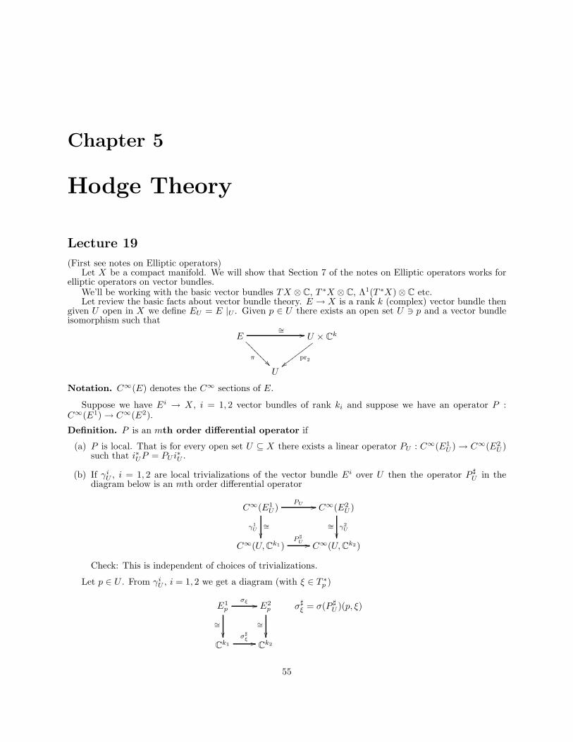
Chapter 5

Hodge Theory

Lecture 19

(First see notes on Elliptic operators) Let X be a compact manifold. We will show that Section 7 of the notes on Elliptic operators works for

elliptic operators on vector bundles. We’ll be working with the basic vector bundles T X ⊗ C, T ∗X ⊗ C, Λ1(T ∗X) ⊗ C etc. Let review the basic facts about vector bundle theory. E X is a rank k (complex) vector bundle then→

given U open in X we define EU = E U . Given p ∈ U there exists an open set U ∋ p and a vector bundle isomorphism such that

|

=∼ ��E × Ck

pr2

U

π

U

Notation. C∞(E) denotes the C∞ sections of E.

Suppose we have Ei X , i = 1, 2 vector bundles of rank ki and suppose we have an operator P : C∞(E1) → C∞(E2).

→

Definition. P is an mth order differential operator if

(a) P is local. That is for every open set U ⊆ X there exists a linear operator PU : C∞(E1 C∞(E2

U ) → U ) such that i∗ P = PU i

∗U U .

(b) If γi U , i = 1, 2 are local trivializations of the vector bundle Ei over U then the operator P ♯ in theU diagram below is an mth order differential operator

C∞(E1 PU �� C∞(E2 U ) U )

1γU = =∼ ∼ 2γU

♯U �� C∞(U, Ck2 ) P

C∞(U, Ck1 )

Check: This is independent of choices of trivializations.

Let p ∈ U . From γi U , i = 1, 2 we get a diagram (with ξ ∈ Tp∗)

♯E1 σξ �� E2

p σξ♯ = σ(PU )(p, ξ)p

= =∼ ∼♯ξσ

��Ck2Ck1

55

�

� ��

� �

�� ��

� �

Definition. σξ = σ(P )(p, ξ)

Check that this is independent of trivialization. f ∈ C∞(U), s ∈ C∞(EU ). Then

(e−itf Pe itf m−1)(p) = tmσ(P )(p, ξ)s(p) + O(t )

where ξ = dfp.

Definition. P is elliptic if k1 = k2 and for every p and ξ = 0 in TpX , then σ(P )(p, ξ) : E1 E2 isp p� →bijective.

5.0.1 Smoothing Operators on Vector Bundles

We have bundles Ei → X . Form a bundle Hom(E1 , E2) → X ×X by defining that at (x, y) the fiber of this

x, E2bundle is Hom(E1 y ). In addition lets let dx be the volume form on X .

Let K ∈ C∞(Hom(E1 , E2)) and define TK : C∞(E1) → C∞(E2), with f ∈ C∞(E1) by

1 2∞ ∞Theorem. P C (E ) C (E )is an th order elliptic differential operator, then there exists an “ th: m m→

��������

TK f(y) = K(x, y)f(x)dx

PQ I−

���������

What does this mean? By definition f(x) ∈ E1 and K(x, y) : E1 E2 x → y , so (K(x, y)f(x)) ∈ E2 . Thus itx y

makes perfect sense to do the integration in the definition.

order ΨDO”, Q : C∞(E2) → C∞(E1) such that

is smoothing.

Proof. Just as proof outlined in notes with Ui, ρi, γi. But make sure that E1 , E2 are locally trivial over Ui, ♯i.e. on Ui, PUi

∼ P ♯ , so PUi is an elliptic system.= Ui

5.0.2 Fredholm Theory in the Vector Bundle Setting

Let E X be a complex vector bundle. Then a hermitian inner product on E is a smooth function→X ∋ p → (, )p where (, )p is a Hermitian inner product on Ep.

If X is compact with s1, s2 ∈ C∞(E) then we can make this into a compact pre-Hilbert space by defining an L2 inner product

s1, s2 = (s1(x), s2(x))dx

Lemma. Given p ∈ X, there exists a neighborhood U of p and a Hermitian trivialization of EU

γU

EU U × Ck

for p ∈ U , Ep ∼ C

k and γU hermitian if Ep ∼ C

k is an isomorphism of hermitian vector spaces.

Proof. This is just Graham-Schmidt

Theorem. Ei → X, i = 1, 2 Hermitian vector bundles and P : C∞(E1) → C∞(E2) an mth order DO, then there exists a unique mth order DO, P t : C∞(E2) → C∞(E1) such that for f ∈ C∞(E1), g ∈ C∞(E2)

= =

�Pf, g�L2 = f, P t g L2

56

U

� � �

� �

Proof. (Using the usual mantra: local existence, local uniqueness implies global existence global uniqueness).

U , E2 ♯So we’ll first prove local existence. Let U be open and γ1

U , γ2 hermitian trivialization of E1

U . P ! PU ,U♯ ♯PU : C

∞(U,Ck1 ) → C∞(U,Ck2 ). Then PU = [Pij ], Pij : C∞(U) → C∞(U), 1 ≤ i ≤ k2, 1 ≤ j ≤ k1.

U )♯ = [P t U )

♯ P t U U ) → U ).Set (P t ji], (P

tU . Then P t : C∞(E2 C∞(E1

U ), g ∈ C0∞(E2We leave the read to check that if f ∈ C0

∞(E1 U ) then

�PU f, g = f, P tU g

This is local existence. Local uniqueness is trivial. This all implies global existence.

Theorem (Main Theorem). X compact, Ei X, i = 1, 2 hermitian bundles of rank k. And P : C∞(E1) → C∞(E2) an m order elliptic DO then

→

(a) ker P is finite dimensional

(b) f ∈ Im P if and only if f, g = 0 for all g ∈ ker P t .

Proof. The proof is implied by existence of right inverses for P modulo smoothing and the Fredholm Theorem for I − T when T : C∞(E1) → C∞(E2).

Lecture 20

C∞(Ek+1X a compact manifold, Ek → X , k = 1, . . . , N complex vector bundles, D : C∞(Ek) → ) first order differential operator. Consider the following complex, hereafter referred to as (∗).

. . . �� C∞(Ek ) D �� C∞(Ek+1)

D �� . . .

is a differential complex if D2 = DD = 0.(∗) For x ∈ X , ξ ∈ T ∗, we have σξ : E

k Ek+1 then we have the symbol σξ (D)(x, ξ). Andx xx →

0 = σ(D2)(x, ξ) = σ(D)(x, ξ)σ(D)(x, ξ)

so we conclude that σ2 = 0. So at every point we get a finite dimensional complexξ

σξ σξ

0 �� E1 �� E2 �� . . . x x

the symbol complex

Definition. (∗) is elliptic if the symbol complex is exact for all x and ξ ∈ T ∗x − {0}.

Examples

(a) The De Rham complex. For this complex the bundle is

Ek : Λk ⊗ C = Λk (T ∗X) ⊗ C

then C∞(Ek ) = Ωk (X). The first order operation is the usual exterior derivative d : C∞(Ek) →C∞(Ek+1). σξ = σ(d)(x, ξ), where σξ : Λ

k (Tx ∗) ⊗ C → Λk+1(Tx

∗) ⊗ C

Theorem. For µ ∈ Λk(Tx ∗) ⊗ C, σξ µ =

√−1ξ ∧ µ.

Proof. ω ∈ Ωk (X), ωx = µ, f ∈ C∞(X), dfx = ξ then

(e−itf de if tω)x = (idf ∧ ω)x + (dω)x = (iξx ∧ µ)t+ (dω)x

57

�

�

� � . . .

� �

Theorem. The de Rham complex is elliptic

Proof. To do this we have to prove the exactness of the symbol complex:

“ “. . . �� Λk(Tx ∗)

∧ξ” �� Λk+1(T ∗ ∧ξ” �� . . . x )

To do this let e1, . . . , en be a basis of T ∗ with e1 = ξ. Then for µ ∈ Λk(Tx ∗), µ = e1 ∧ α + β where αx

and β are products just involving e2, . . . , en (this is not hard to prove).

(b) Let X be complex and let us define a vector bundle

Ω0,k(X)Ek = Λ0,k(T ∗) C∞(Ek ) =

Take D = ∂. This is a first order DO, ∂ : C∞(Ek ) → C∞(Ek+1), σxi = σ(D)(x, ξ), now what is this symbol?

Take ξ ∈ T ∗, then ξ = ξ1,0 + ξ0,1 where ξ1,0 ∈ (T astx)1,0 , ξ0,1 ∈ (Tx

∗)0,1 and ξ1,0 = ξ 0,1

, ξ = 0 thenx ξ0,1

�= 0.

Theorem. For µ ∈ Λ0,ki(Tx ∗), σξ (µ) =

√−1ξ0,1 ∧ µ.

Proof. ω ∈ Ω0,k(X), ωx = µ, f ∈ C∞(X), dfx = ξ then

(e−itf ∂e itf ω)x = (it∂f ∧ ω)xt+ (∂ω)x = itξ0,1 ∧ µ+ ∂ωx

Check: For ξ = 0 the sequence

. . . �� Λ0,k(T ∗ “∧ξ0,1

��” Λ0,k+1(Tx ∗“)∧ξ0,1” ���� . . .

x )

is exact. This is basically the same as the earlier proof, when we note that Λ0,k(Tx ∗) = Λk((Tx

∗)0,1). we conclude that the Dolbeault complex is elliptic.

(c) The above argument forks for higher dimensional Dolbeault complexes. If we set

Ωp,k(X)Ek = Λp,k(T ∗X), D = ∂, C∞(Ek ) =

it is easy to show that σ(∂)(x, ξ) = “ ∧ ξ0,1”

The Hodge Theorem

Given a general elliptic complex

. . . D �� C∞(Ek ) D �� C∞(Ek+1)

D

with dx a volume form on X , equip each vector bundle Ek with a Hermitian structure. We then get an L2

inner product , L2 on C∞(Ek ). And for each D : C∞(Ek ) → C∞(Ek+1) we get a transpose operator

Dt : C∞(Ek+1 C∞(Ek )) →

If for x ∈ X , ξ ∈ Tx ∗, σξ = σ(D)(x, ξ) then

σ(Dt)(x, ξ) = σt x

58

So we can get a complex in the other direction, call it (∗)t

Dt Dt

. . . �� C∞(Ek ) Dt

�� C∞(Ek−1) �� . . .

and since 0 = (Dr )t = (DD)t = DtDt = (Dt)2 we have that (∗)t is a differential complex. Also, σ(Dt)(x, ξ) = σξ = σ(D)(x, ξ)t . For x and ξ ∈ T ∗ − {0} the symbol complex of Dt isx

σt σt ξ

0 �� EN ξ �� EN −1 �� . . . x x

The transpose of the symbol complex for D. So (∗) elliptic implies that (∗)t is elliptic.

Definition. The harmonic space for (∗) is

k = s ∈ C∞(Ek ), Ds = s = 0}H { Dt

Theorem (Hodge Decomposition Theorem). We have two propositions

(a) For all k, Hk is finite dimensional.

(b) Every element u of C∞(Ek ) can be written uniquely as a sum u1 + u2 + u3 where u1 ∈ Im(D), ku2 ∈ Im(Dt), u3 ∈ H

Before we prove this we’ll do a little preliminary work. Let

N

E = �

Ek

k=1

Then consider the operator D + Dt : C∞(E) → C∞(E)

Check: This is elliptic.

Proof. Consider Q = (D + Dt)2 . It suffices to show that Q is elliptic.

Q = D2 + DDt + DtD + (Dt)2

but the two end terms are 0. So Q = DDt + DtD

Note that Q sends C∞(Ek ) to C∞(Ek ), so Q behaves nicer than D + Dt . So now we want to show that Q is elliptic.

Let x, ξ ∈ Tx ∗ . Then− {0}

σ(Q)(x, ξ) = σ(DDt)(x, ξ) + σ(DtD)(x, ξ) = σt ξξ + σξ σt

x ξ

(where σξ = σ(D)(x, ξ).

Suppose v ∈ Ek and σ(Q)(x, ξ)v = 0 (i.e. it fails to be bijective). Thenx

((σξt σξ + σξ σξ

t )v, v) = 0 = (σξ v, σξ v)x + (σξt v, σξ

t v) = 0

which implies that σξ v = 0 and σξt v = 0. Now σξ = 0 implies that v ∈ Im σξ : E

k−1 Ek by exactness. Wex → x

know that Im σξ ⊥ ker σξt , but v ∈ ker σξ

t , so v⊥v implies that v = 0.

So Q is elliptic and thus (D + Dt) is elliptic.

Lemma. Hk = ker Q.

59

� � � � �

� � � �

� �

Proof. We want to show Hk ⊆ ker Q. The other direction is easy. Let u ∈ ker Q. Then

�DDt u + DtDu, u = 0 = Dt u, Dt u + Du, Du = 0

kThis implies that Dtu = Du = 0, so .u ∈ H

Proof of Hodge Decomposition. By the Fredholm theorem every element u ∈ C∞(Ek ) is of the form u = v1 + v2 where v1 ∈ Im(Q) and v2 ∈ ker Q. v2 ∈ ker Q implies that v2 ∈ Hk , v1 ∈ Im Q implies that v1 = Qw = D(Dtw) + Dt(Dw). Choose u1 = DDtw, u2 = DtDw and v2 = u3.

Left as an exercise: Check that u = u1 +u2 +u3 is unique. Hint: ker D⊥ Im Dt and ker Dt⊥ Im D. Then the space Im(D), Im(Dt) and H are all mutually perpendicular.

Lecture

The Hodge ∗-operator

Let V = V n be an n-dimensional R-vector space. Let B : V × V R be a non-degenerate bilinear form on→V (Note that for the momentum we are not assuming anything about this form).

From B one gets a non-degenerate bilinear form B : Λk(V ) × λk (V ) → R. If α = =v1 ∧ · · · ∧ vk,β w1 ∧ · · · ∧ wk then

B(α, β) = det(B(vi, vj ))

Alternate definition: Define a pairing (non-degenerate and bilinear) Λk (V )×Λk(V ∗) → R with α =

vi ∈ V , fi ∈ V ∗v1∧· · ·∧vk, β = f1∧· · ·∧fk,

. Thenα, β = d vi, fj

This gives rise to the identification Λk(V ∗) ∼ Λk(V )∗.= =

So B : V × V R gives to LB : V ∼V ∗ by B(u, v) = u, LB v . This can be extended to a map of k-th→ −→

exterior powers, LB : Λk (V ) → Λk (V ∗), defined by

� �

=LB (v1 ∧ · · · ∧ vk ) LB v1 ∧ · · · ∧ LB vk

and if we have α, β ∈ Λk (V ) then B(α, β) = α, LB β . Let us now look at the top dimensional piece of the exterior algebra. dim Λn(V ) = 1, orient V so that

we are dealing with Λk(V )+. Then there is a unique Ω ∈ Λn(V ) such that B(Ω, Ω) = 1.

Theorem. There exists a bijective map ∗ : Λk (V ) → Λn−k (V ) such that for α, β ∈ Λk (V ) we have

B(α, β)Ωα ∧ ∗β =

= Proof. From Ω we get a map Λn(V )

∼So we get a non-degenerate pairing−→ R, λΩ �→ λ.

Λk (V ) × Λk (V ) → Λn(V ) → R

Now we have a mapping Λk (V ∗) k

Λn−k (V ). Define the ∗-operator to be k LB .−→ ◦

There is a clear dependence of ∗ on the orientation of V . If we exchange Ω for −Ω then ∗ turns to −∗. Lets say something about the dependence on B.

Suppose we have B1, another non-degenerate bilinear form on V . Then there exists a unique J : V cong −−−→ V

so that B1(u, v) = B(u, Jv). In fact we define J by requiring that LB1 : V V ∗ is given by setting

LB1 = LB J .

→

Extend◦J to a map J : Λk (V ) → Λk (V ) by setting J(v1 ∧ · · · ∧ vk ) = Then on Λk(V ),Jv1 ∧ · · · ∧ Jvk .

LB1 = LB = k LB1

= k LB J = So the star operator for B1 and B are relation b ∗1 = ◦J , ∗1 ◦ ◦ ◦ ∗◦J . ∗◦J .

60

21

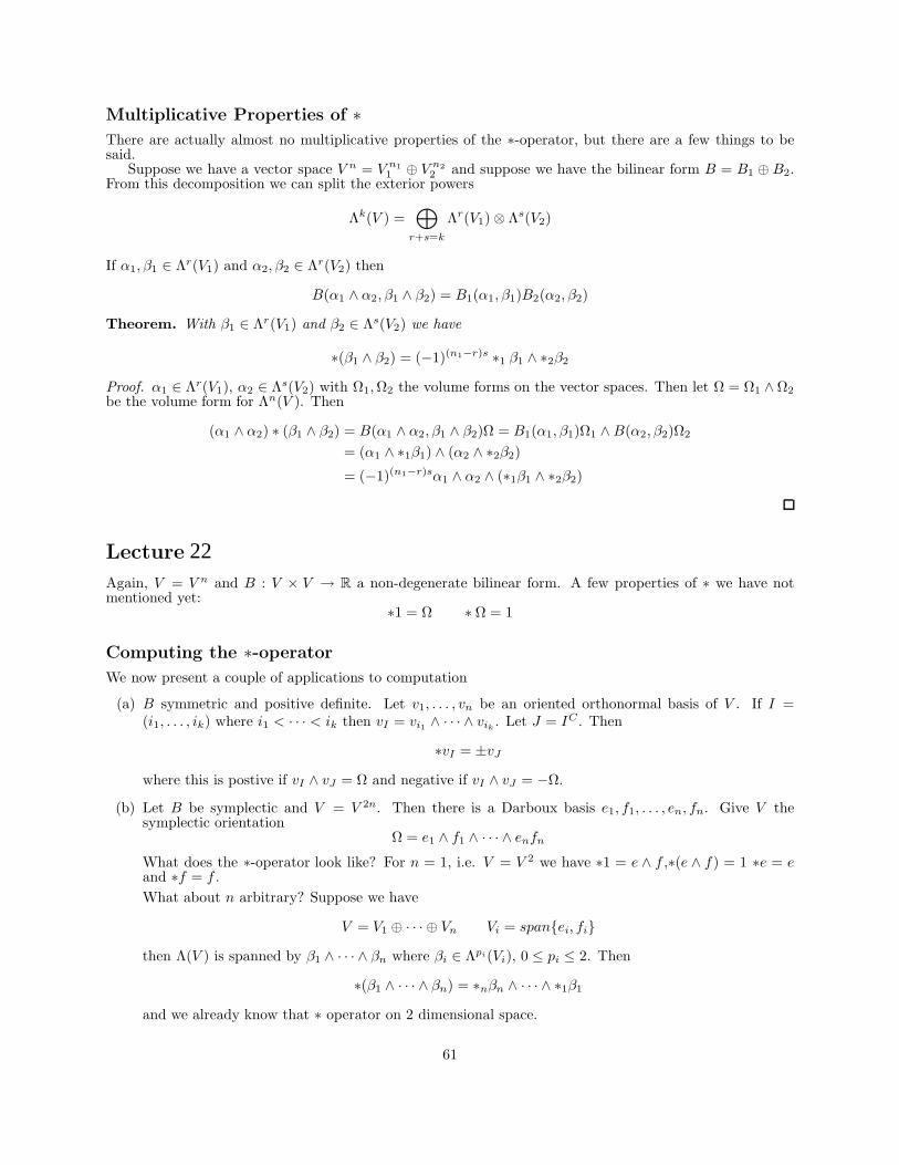
Multiplicative Properties of ∗ There are actually almost no multiplicative properties of the ∗-operator, but there are a few things to be said.

Suppose we have a vector space V n = V n1 ⊕ V n2 and suppose we have the bilinear form B = B1 ⊕ B2.1 2 From this decomposition we can split the exterior powers

Λk(V ) = �

Λr(V1) ⊗ Λs(V2) r+s=k

If α1, β1 ∈ Λr(V1) and α2, β2 ∈ Λr(V2) then

B(α1 ∧ α2, β1 ∧ β2) = B1(α1, β1)B2(α2, β2)

Theorem. With β1 ∈ Λr (V1) and β2 ∈ Λs(V2) we have

∗(β1 ∧ β2) = (−1)(n1−r)s 2β2∗1 β1 ∧ ∗

Proof. α1 ∈ Λr(V1), α2 ∈ Λs(V2) with Ω1,Ω2 the volume forms on the vector spaces. Then let Ω = Ω1 ∧ Ω2 be the volume form for Λn(V ). Then

(α1 ∧ α2) ∗ (β1 ∧ β2) = B(α1 ∧ α2, β1 ∧ β2)Ω = B1(α1, β1)Ω1 ∧B(α2, β2)Ω2

= 2β2)(α1 ∧ ∗1β1) ∧ (α2 ∧ ∗= (−1)(n1−r)sα1 ∧ α2 ∧ (∗ 2β2)1β1 ∧ ∗

Lecture

Again, V = V n and B : V × V R a non-degenerate bilinear form. A few properties of ∗ we have not mentioned yet:

→

= Ω ∗ Ω = 1∗1

Computing the ∗-operator

We now present a couple of applications to computation

(a) B symmetric and positive definite. Let v1, . . . , vn be an oriented orthonormal basis of V . If I = (i1, . . . , ik ) where i1 < < ik then vI = vi1 ∧ · · · ∧ vik

. Let J = IC . Then · · ·

vI = vJ∗ ±

where this is postive if vI ∧ vJ = Ω and negative if vI ∧ vJ = −Ω.

(b) Let B be symplectic and V = V 2n . Then there is a Darboux basis e1, f1, . . . , en, fn. Give V the symplectic orientation

Ω = nfne1 ∧ f1 ∧ · · · ∧ eWhat does the ∗-operator look like? For n = 1, i.e. V = V 2 we have ∗1 = e ∧ f ,∗(e ∧ f) = 1 ∗e = e and ∗f = f .

What about n arbitrary? Suppose we have

V = n Vi = span{ei, fi}V1 ⊕ · · · ⊕ V

then Λ(V ) is spanned by β1 ∧ · · · ∧ βn where βi ∈ Λpi (Vi), 0 ≤ pi ≤ 2. Then

n) = nβ 1β1∗(β1 ∧ · · · ∧ β ∗ n ∧ · · · ∧ ∗

and we already know that ∗ operator on 2 dimensional space.

61

22

Other Operations

For u ∈ V we can define an operation Lu : Λk → Λk+1 by α �→ u ∧ α. We can also define this operations

dual: for v∗ ∈ V ∗, iv ∗ : Λk Λk−1 the usual interior product. →

But because we have a bilinear form we can find Lt and it ∗ and since we have ∗ we have other interesting u v things to do, like conjugate with the ∗-operator:

∗−1Lu ∗ ∗−1(iv ∗ )∗

Theorem. For α ∈ Λp−1 , β ∈ Λp

B(Luα, β) = B(α,Lt β)u

where Lt = (−1)p−1 ∗−1 Lu∗ := �Lu.u

Proof. Begin by noting Lu = B(Luα, β)Ω. Now α ∧ ∗β

= (−1)p−1α ∧ u ∧ ∗β =u ∧ α ∧ ∗β (−1)pα ∧ ∗(∗−1 u ∧ ∗β)

= Luβ = B(α, �Luβ)Ω α ∧ ∗�

which implies that �Lu = Lt .u

What is this transpose really doing? We know we have a bilinear form B that gives rise to an map Lu : V V ∗. Since B is not symmetric, define B♯(u, v) = B(v, u), and we get a new map LB♯ : V V ∗.→ →Then:

∗ .Theorem. If v∗ = LB♯u, then Lt = ivu

Proof. Let u1, . . . , un be a basis of V and let v1, . . . , vn be a complementary basis of V determined by

B(ui, vj ) = δij

and let v∗ n 11 , . . . , v∗ be a dual basis of V ∗. Check that v∗ = LB♯ u1. Let I = (i1, . . . , ik−1) and J = (j1, . . . , jk)

be multi-indices. We claim that B(L uI , vJ ) = B(uI , iv ∗ vJ )u1 1

and that if j1, . . . , jk = 1 and i1, . . . , ik−1 = 1 then both sides are 1. Otherwise they are 0.

Theorem. On Λp+1 , (iv ∗ )t = (−1)p ∗−1 (iv ∗ )∗ and v∗ = LB u.

Lecture

For the next few days we’re assuming that B is symplectic and V = V 2n . Choose a Darboux basis e1, f1, . . . , en, fn. Check that LB : V V ∗ is the map →

i , fi{ei → −f∗ → ei ∗}

where e∗i , f∗ are the dual vectors. In the symplectic case B♯ = −B and LB♯ = −L.i

Say that ω ∈ Λ2V ,

ω = �

ei ∧ fi

Λp

Lets look at the commutator [L,Lt] : Λp Λp. →Then we have the operation L : Λp → Λp+2 , given by α �→ ω ∧ α and also its transpose Lt : Λp+2 .

→

Theorem (Kaehler, Weil). [L,Lt] = (p− n) Id

62

23

�

�

Proof. L = �

i Lei Lfi

, so

Lt = �

Lt Lt = �

ιf ∗ ιe ∗ fi ei i i

i

Its easy to see that Kaehler-Weil holds when n = 2. For n-dimensions

L = �

Li Li = Lei Lfi

Lt = �

Lt i Lt i = ιf ∗ i ιe ∗ i

Vi = span{ei, fi}, then Λp = spanβ1 ∧ · · · ∧ βn where βi ∈ Λpi (Vi). Note that

=Liβ1 ∧ · · · ∧ βn β1 ∧ · · · ∧ (Liβi) ∧ · · · ∧ βn

and Lt = j (β1 ∧ · · · ∧ βn) β1 ∧ · · · ∧ (Lj βj ) ∧ · · · ∧ βn

If n = j, then LiLt = Lt Li. So j j

[L, Lt]β1 ∧ · · · ∧ βn = �

β1 ∧ · · · ∧ [Li, Lti]βi ∧ · · · ∧ βn

i n

= =�

(pi − 1)β1 ∧ · · · ∧ βn (p − n)β1 ∧ · · · ∧ βn

Lecture

Proposition. Lt = ∗−1L∗ Proposition. u ∈ V then [Lt u, L] = −Lu. Proof. Proof omitted.

Let (X2n, ω) be a compact symplectic manifold. Let x ∈ X and V = T ∗. Notice x

(a) From ωx we get a symplectic bilinear form on Tx.

(b) From this form we get an identification Tx T ∗.x→(c) Hence from 1, 2 we get a symplectic bilinear from Bx on V .

(d) From Bx we get a ∗-operator∗x : Λ

p(Tx ∗) → Λ2n−p(Tx

∗)

(e) This gives us a ∗-operator on forms

∗ : Ωp(X) → Ω2n−p(X)

We can define a symplectic version of the L2 inner product on Ωp as follows. Take α, β ∈ Ωp and define

α, β =� �X α ∧ ∗β

(Note: This is not positive definite or anything, its just a pairing) Take α ∈ Ωp−1 , β ∈ Ωp. Then look at

= dα ∧ ∗β + (−1)p−1α ∧ d ∗ βd(α ∧ ∗β)

= dα ∧ ∗β + (−1)p−1α ∧ ∗(∗−1d∗)β

63

24

� �

� � � �

� �� �

X

x

Since �

d(α ∧ ∗β) = 0, we integrate both sides of the above and get

= (−1)p

X dα ∧ ∗β α ∧ ∗(∗−1d∗)β

If we introduce the notation δ = (−1)p ∗−1 d∗ on Ωp then

dα, β = α, δβ

Now, given the mapping L : Ωp → Ωp+2 , Lα = ω ∧ α we have the following theorem

Theorem. [δ, L] = d.

This identity has no analogue in ordinary Hodge Theory. This is very important.

Proof. x ∈ X , ξ ∈ T ∗, then σ(d)(x, ξ) = iLξ. On Λp, δ = (−1)p∗−1d∗, so σ(d)(x, ξ) = (−1)pi∗−1Lξ ∗ = −iLt x ξ. Then

σ([δ, L]) = i[Lt ξ, L] = iLξ = σ(d)(x, ξ)

so [δ, L] and d have the same symbol. Now, d [δ, L] are first order DO’s mapping Ωp → Ωp+1 , so d − [δ, L] : Ωp Ωp+1 is a first order DO. We →

want to show that this is 0. Let (U, x1, . . . , xn, y1, . . . , yn) be a Darboux coordinate patch. Consider u = where βi =

1, dxi, dyi or dxi ∧ dyi. β1 ∧ · · · ∧ βn

These de Rham forms are a basis at each point of Λ(Tx ∗).

Lu = ω ∧ u is again a form of this type since ω = � dxi ∧ dyi is of this form. Also ∗u i s of this from.

Note that d = 0 on a form of this type, hence δ = ∗−1d∗ is 0 on a form of this type. Thus [δ, L]− d is 9 on a form of this type.

Lecture

Symplectic Hodge Theory

(X2n, ω) be a compact symplectic manifold. From x ∈ X we get ωx Bx a non-degenerate bilinear form on T ∗, and so induces a non-degenerate bilinear from on Λp(Tx

∗). →

Define , L2 on Ωp as follows. Take Ω = ωn/n!, a symplectic volume form, α, β ∈ Ωp

α, β = Bx(α, β)Ω =� �X X

α ∧ ∗β

Remarks:

(a) In symplectic geometry ∗2 = id, ∗ = ∗−1 .

(b) �, � is anti-symmetric on Ωp, p odd and symmetric on Ωp, p even.

(c) [Lt, δt] = dt = δ. And δt = (dt)t = −d, so [d, Lt] = δ.

Consider the Laplace operator dδ + δd = ddt + dtd. Now, in the symplectic world, Δ = 0. We’ll prove this: δ = [d, Lt] = dLt − Ltd, so dδ = −dLtd and δd = dLtd, so Δ = 0.

So for symplectic geometry we work with the bicomplex (Ω, d, δ). We’re going to use symplectic geometry to prove the Hard Lefshetz theorem for Kaehler manifolds.

Let (X2n, ω) be a compact Kaehler manifold. Then we have the following operation in cohomology

γ : Hp(X, C) → Hp+2(X) c �→ [ω] ⌣ c

Theorem (Hard Lefshetz). γp is bijective.

Question: Is Hard Lefshetz true for compact symplectic manifolds. If not, when is it true. Define [Lt, L] = A, by Kaehler-Weil says that Aα = (n − p)α.

Lemma. [A, Lt] = 2Lt .

Proof. ALtα − LtAα = (n − (p − 2))Ltα − (n − p)Ltα = 2Lta

Lemma. [A, L] = −2L.

There is another place in the world where you encounter these: Lie Groups.

64

25

�

Lie Groups

Take G = SL(2, R), then consider the lie algebra g = sl(2, R). This is the algebra {A ∈M22(R), tr A = 0}. Generated by

�0 1

� �0 1

� �1 0

�

X = Y = H = 0 0 1 0 0 −1

Check that [X, Y ] = H , [H, X ] = 2X and [H, Y ] = −2Y , and sl(2, R) = span{X, Y, Z}, and the above describes the Lie Algebra structure.

ρ : g → End(Ω) be given by X �→ Lt , Y �→ L and H �→ A is a representation of the Lie algebra g on Ω. So Ω is a g-module.

Lemma. Ωharm is a g-module of Ω.

Proof. First note that Ld = dL, i.e. dLα = d(ω ∧ α) = ω ∧ dα = Ldα. Taking transposes we get Ltδ = δLt . Then take α ∈ Ωharm. We already know that [d, Lt] = δ, so dLtα−Ltdα = δα, which implies that dLtα = 0. Similarly dLα, δLα = 0, so Lα, Ltα are in Ωharm.

So since A = [L, Lt], Aα ∈ Ωharm and Ω is a g-module.

Note that Ωharm is not finite dimensional. So these representations are not necessarily easy to deal with.

Definition. Let V be a g-module. V is of finite H-type if

N

V = �

Vi i=1

and H = λiId on Vi.

In other words, H is in diagonal form with respect to this decomposition.

ΩpExample. Ω = �2n

Ωp, H = (n − p)Id on Ωp and Ωharm = �2n

harm, H = (n − p)Id on Ωp p=0 p=0 harm .

Theorem. If V is a g-module of finite type, then every sub and quotient module is of finite type. �N

Proof. V = i=1 Vi, H = λiId on Vi. Let πi : V Vi be a projection onto Vi. Check that → 1

πi = �(λi − λj )

�(H − λj )

j=i

i.e., πiv = v on vi. So πi takes sub/quotient objects onto themselves.

Lecture

Lemma. Take v ∈ V , Hv = λv. We claim that H(Xv) = (λ + 2)Xv.

Proof. (HX −XH)v = 2Xv, so HXv = λXv + 2Xv = (λ + 2)Xv.

Lemma. If Hv = λv, then [X, Y k ]v = k(λ − (k − 1))Y k−1 v

Proof. We proceed by induction. If k = 1 this is just [X, Y ]v = Hv = λv. This is true. Now we show that if this is true for k, its true for k + 1.

[X, Y k+1]v = XY k+1 v − Y k+1Xv

= (XY )Y k v − (Y X)Y k v + Y (XY k )v − Y (Y k Xv)

= HY k v + Y ([X, Y k ])v

= (λ − 2k)Y k v + Y (k(λ − (k − 1))Y k−1 v

= ((λ − 2k) + k(λ − k − 1))Y k v = (k + 1)(λ − k)Y k v

65

26

�

�

�

Definition. V is a cyclic module with generator v if every submodule of V containing v is equal to V itself.

Theorem. If V is a cyclic module of finite H type then dim V < ∞.

Proof. Let v generate V . Then v = �Ni=0 vi where vi ∈ Vi. It is enough to prove the theorem for cyclic

modules generated by vi. We can assume without loss of generality that Hv = λv. Now, note that only a finite number of expression Y k X lv are non-zero (since X shifts into a different

eigenspace, and there are only a finite number of eigenspaces). By the formula that we just proved, span{Y k X lv} is a submodule of V containing v.

Fact: Every finite dimensional g-module is a direct sum of irreducibles. In particular, every cyclic submodule of V is a direct sum of irreducibles.

Theorem. Every irreducible g-module of finite H type is of the form V = where dim Vi = 1. Moreover, there exists vi ∈ Vi − {0} such that

V0 ⊕ · · · ⊕ Vk

Hvi = (k − 2i)vi Y vi = vi+1 i ≤ k − 1

Xvi = i(k − (i − 1))vi−1 i ≥ 1

Xv0 = 0, Y vk = 0

Proof. Let V = V0 ⊕ · · · ⊕ Vn, and H = λiId on Vi and assume that λ0 > λ1 > > λn. Take . Note that Xv = 0, because HXv = (λ0 + 2)Xv and λ0 + 2 > λ0.

· · · v ∈ V0 −{0}

Consider Y v, . . . , Y k v = 0, Y k+1v = 0, so HY iv = (λ0 − 2i)Y iv. and

XY i v = Y iXv + i(λ − (i − 1))Y i−1 v = i(λ − (i − 1))Y i−1 v

When i = k + 1 we have XY k+1 v = 0 = (k + 1)(λ − k)Y k v

but Y k v = 0, so it must be that λ = k. Now just set vi = Y iv.

Lemma. Let V be a k + 1 dimensional vector space with basis v0, . . . , vk . Then the relations in the above theorem define an irreducible representation of g on V

Definition. V a g-module, V = �N

Vi of finite H-type. Then v ∈ V is primitive if i=0

(a) v is homogenous,(i.e. v ∈ Vi)

(b) Xv = 0.

Theorem. If v is primitive then the cyclic submodule generated by v is irreducible and Hv = k where k is the dimension of this module.

Proof. v, Y v, . . . , Y k v = 0, Y k+1 = 0. Take vi = Y iv. Check that vi satisfies the conditions.

Theorem. Every vector v ∈ V can be written as a finite sum

� Y l vlv =

where vl is primitive.

Proof. This is clearly true if V is irreducible (by the relations). Hence this is true for cyclic modules, because they are direct sums of irreducibles, hence this is true in general.

Corollary. The eigenvalues of H are integers.

Proof. We need to check this for eigenvectors of the form Y lv where v is primitive. But for v primitive we know the theorem is true, i.e. Hv = kv, HY lv = (k − 2l)Y lv. So write V =

� Vr , H = rId on Vr

66

Lecture

Theorem. We can repagenate the sum so that

N

V = �

Vi i=−N

where

H = iId on Vi

(a) X : Vi Vi+2 and Y : Vi+2 Vi.→ →

(b) Y iVi cong

V−i is bijective.−−−→

Now, recall that we are going to apply this stuff to Hodge Theory. In particular, let (X2n , ω) be a symplectic, compact manifold. Then we define L : Ωk (X) → Ωk+2(X) given by α �→ ω ∧α, ∗ : Ωk Ω2n−k ,→Lt : Ωk+2 Ωk given by Lt = ∗L∗ and we defined A : Ω ω, A = iId on Ωn−i . The Kaehler-Weil identities→ →said that

[Lt , L] = A [A, Lt] = 2Lt [A, L] = −2L

So Ω is a g-module of finite H-type with X = Lt , Y = L and H = A.

Corollary. The map Lk : Ωn−k Ωn+k is an isomorphism.→ We can apply this to symplectic hodge theory as follows. We know in this case that

[d, Lt] = δ [δ, L] = d

Let Ωharm = {u ∈ Ωdu = δ = 0}. Theorem. Ωharm is a g-module of Ω.

Ωn+kCorollary. The map Lk : Ωn−k harm → harm is bijective.

Hard Lefshetz Theorem

ω ∈ Ω2 , dω = 0. Then [ω] defines a cohomology class [ω] ∈ H2 = H2(X). And in turn we can define aDR(X) mapping γ : Hk (X) → Hk+2(X) by c �→ [ω] ⌢ c.

Theorem. Let X be Kaehler then γk : Hn−k (X) → Hn+k(X) is bijective.

What about the symplectic case? Let u ∈ Ωk with du = 0. Define a mapping Pk : Ωk Hk(X)harm harm →

by u �→ [u] Theorem. (Matthieu) Hard Lefshetz holds for X if and only if Px is onto for all k.

Proof. The “only if” part is covered in the supplementary notes. Now the for the “if” part, we use the following diagram

Ωn−kLk

�� Ωn+k harm harm

��γk ��

Hn−k(X) �� Hn+k (X)

Lk is bijective, the vertical arrows are surjective, so γk is surjective. Poincare duality tells us that dim Hn−k = dim Hn+k so γk is bijective.

Remarks:

(a) “if” condition is automatic for Kaehler manifolds

67

27

� �

� � . . .

= (b) A consequence of Hard Lefshetz. We know that H2n(X)

∼R given by [u] �→

�u is (by stokesX−→

theorem) bijective. Hence one can define a bilinear form on Hn−k(X) via

= c1, c2 γk c1 ⌢ c2 ∈ H2n(X)

∼R→ −→

By poincare and hard lefshetz this form is non-degenerate, i.e. γk c1 ⌢ c2 = 0 for all c2, then by Poincare γkc1 = 0 which implies that c1 = 0.

A consequence is that for k odd Hk(X) is even dimensional.

(c) Thurston showed that there exists lots of compact symplectic manifolds with dim H1(X) odd, i.e. it doesn’t satisfy strong lefshetz.

(d) For any symplectic manifold X , let Hk symp(X) = Im(Ωk Hk(X)). For symplectic cohomologyharm →

you do have Hard Lefshetz.

Riemannian Hodge Theory

Let V = V n be a vector space over R. B is a positive definite inner product on V . Assume V is oriented, then you get ∗ : Λk(V ) → Λn−k(V ). Take v1, . . . , vn to be an oriented orthonormal basis of V . I = (i1, . . . , ik), i1 < < ik. Ic the complementary multi-index. Then ∗vI = ǫvIc where ǫvI ∧ vIc = n (where ǫ· · · is some sign).

v1 ∧ · · · ∧ v

Let X = Xn be a compact Riemannian manifold. From the Riemannian metric we get Bp a positive definite inner product on T ∗ so Bp induces a positive definite inner product on Λk(Tp

∗).p

From these inner products we get the star operator ∗p : Λk → Λn−k satisfying α, β ∈ Λkp p p , α ∧ ∗β =

Bp(α, β)vp where vp is the Riemannian volume form.

p ⊗C and ∗p extends C-linearly to ΛkIts clear that Bp extends C-linearly to a C-blinear form on Λk p ⊗ C. ¯ ¯A hermitian inner product on Λk (Tp

∗) ⊗ C by (α, β)p = Bp(α β) and α ∧ ∗β := (α, β)p vp.

Globally, Ωk(X) = C∞(Λk(T ∗X) ⊗ C). Define an L2 inner-product by α, β ∈ Ωk(X)

¯α, β = (α, β)p v = β� �X X

α ∧ ∗

dFrom Ω0(X)

d Ω1(X) . . . we get an elliptic complex→ −− →

C∞(X) �� C∞(Λ1(T ∗X) ⊗ C)

We have a hermitian inner product on the vector bundles Λk (T ∗X) ⊗ C, so we can get a transpose

dt : C∞(Λk (T ∗X) ⊗ C) → C∞(Λk−1(T ∗X) ⊗ C)

and write dt = δ and think of δ as δ : Ωk Ωk−1 .→Form the corresponding Laplacian operator Δ = dδ + δd.Apply the general theory of Elliptic complexes to this case. We conclude that

(a) Hk = {u ∈ Ωk ,Δu = 0} is finite dimensional.

(b) Hk = {u ∈ Ωk , du = δu = 0}. (c) Hodge Decomposition

Ωk = {(Im d) ⊕ (Im δ) ⊕Hk}

(d) The map Hk Hk → DR is bijective, i.e. every cohomology class has a unqiue harmonic representation.

Lecture

The Hk are finite-dimensional.DR

68

28

�

� ¯

�

� � � �

�

Poincare Duality

Make a pairing P : Ωk × Ωn−k C given by →

P (α, β) = α ∧ β X

If α is exact and β closed then P (α, β) = 0, since α = dω, dβ = 0 and α ∧ β = du ∧ β = d(u ∧ β). By stokes � α ∧ β is thus 0. P induces a pairing in cohomology, P ♯ : Hk C.DR ×Hn−k

DR →

Theorem (Poincare). This is a non-degenerate pairing.

We give a Hodge Theoretic Proof. First,

Lemma. δ : Ωk → Ωk−1 is given by δ = (−1)k ∗−1 d∗

Proof. Let δ1 = (−1)k ∗−1 d∗, we want to show that δ = δ1. Let α ∈ Ωk−1 and β ∈ Ωn−k then

¯ ¯ ¯d(α ∧ β) = dα ∧ β + (−1)k−1α ∧ d ∗ β ¯ ¯= dα ∧ ∗β + (−1)k−1α ∧ ∗(∗−1d ∗ β)

¯= dα ∧ ∗ β − α ∧ ∗(δ1β)

Now integrate and apply stokes

β =dα ∧ ∗ α ∧ ∗δ1β

so dα, β = α, δ1β and δ1 = dt = δ.

Corollary. ∗Hk = Hn−k

Proof. Take α ∈ Hk . We’ll show that d ∗ α = 0. This happens iff ∗−1d ∗ α = ±δα. Since δα = 0, d ∗ α = 0. It is similarly easy to check that δ ∗ α = 0.

Proof of Poincare Duality. If suffices to check that the pairing P : Hk C given by α, β �→�X α∧β×Hn−k →

is non-degenerate. Suppose P (α, β) = 0 for all β. Take β = α. Then ∗¯

P (α, β) = α = α, α = 0 X α ∧ ∗¯ � �

so this would imply that α = 0.

A Review of Kaehlerian Linear Algebra

Definition. V = V 2n a vector space over R, Bs a non-degenerate alternating bilinear form on V , J : V V a linear map such that J2 = −I. Bs and J are compatible if Bs(Jv, Jw) = Bs(v, w).

→

Lemma. If Bs and J are compatible if and only if the bilinear form Br(v, w) = Bs(v, Jw) is symmetric. (Here Br is a Riemannian metric)

J,Bs Kaehler implies that Br is positive definite. Notice that Br(Jv, Jw) = Bs(Jv, J

2w) = Bs(v, Jw) = Br(v, w) so that Br and J are compatible. And also notice that Br(Jv, w) = Bs(Jv, Jw) = Bs(v, w). Let J t be the transpose of J with respect to Br Then

Br(Jv, Jw) = Br(v, JtJw) = Br(v, w)

so J tJ = I and J t = −J .

69

Br, Bs, J in Coordinates

Let e ∈ V such that Br(e, e) = 1, and set f = Je, and e = −Jf . Then

Br (e, e) = 1 Bs(e, f) = 1

Take V1 = span{e, f}. This is a J-invariant subspace. If we then take

V1⊥ = orthocomplement of V1 w.r.t Br

then for v ∈ V1, w ∈ V1⊥, 0 = Br(Jv, w) = Bs(v, w), so V1

⊥ is the symplectic orthocomplement of V1 with respect to Bs.

Applying induction we get a decomposition

V = V1 ⊕ V2 ⊕ · · · ⊕ Vn

where Vi = span{ei, fi} such that e1, f1, . . . , en, fn is an oriented orthonormal basis of V with respect to Br and a Darboux basis with respect to Bs. Note that Jei = fi and Jfi = ei−

5.0.3 Br, Bs and J on Λk(V )

ω = � ei ∧ fi is the symplectic element in Λ2(V ) and Ω = ωn/n! = is the symplectic e1 ∧ f1 ∧ · · · ∧ en ∧ fn

volume for and Riemannian volume form. On decomposable elements, α = v1 ∧ · · · ∧ vk and β = w1 ∧ · · · ∧ wk and

Br (α, β) = det(Br (vi, wj )) Bs(α, β) = det(Bs(vi, wj ))

and we can define Jα = Jv1 ∧ · · · ∧ Jvk

Notice that Br (α, β) = det(Br (vi, wj )) = det Bs(vi, Jwj ) = Bs(α, Jβ)

and furthermore, it is easy to check that Br(Jα, Jβ) = Br (α, β), Bs(Jα, Jβ) = Bs(α, β), J2 = (−1)kId and if J t : Λk → Λk is the Br -transpose of J , then J t = (−1)k J .

The Star Operators

These are ∗r and ∗s, the Riemannian and symplectic star operators, respectively. Let Ω be the symplectic (and Riemannian) volume form. For α, β ∈ Λk we have

rβ = Br (α, β)Ω = Bs(α, Jβ) = sJβ α ∧ ∗ α ∧ ∗so

r = sJ∗ ∗Also, notice that

r Jβ = Br(Jα, Jβ)Ω = Br (α, β)Ω = rβJα ∧ ∗ α ∧ ∗on the other hand JΩ = Ω, so

rβ = Br (α, β)Ω = Jα ∧ ∗rJ ∗r βα ∧ ∗so ∗rJ = r and since ∗r = sJ we have J∗s = sJ .J∗ ∗ ∗

Structure of Λ(V )

We have a symplectic element ω = � ei ∧fi ∈ Ω2 . From this, we can define a mapping L : Λk Λk+2 given

Note that by α �→ ω ∧ α. LJα = ω ∧ Jα = J(ω ∧ α) = JLα

→

so that [J, L] = 0. Similarly for Lt : Λk+2 Λk , the symplectic transpose given by Lt = s s. Since ∗s, L commute with L∗→

the J map, so does Lt, so [J, Lt] = 0. ∗

Notice that

Br (Lα, β) = Bs(Lα, Jβ) = Bs(α,LtJβ) = Bs(α, JL

tβ) = Br (α,Ltβ)

so Lt is also the Riemannian transpose. From L,Lt we get a representation of SL(2,R) on Λ(V ) and this representation is J-invariant.

70

� � � �� �

� �

� �

Lecture

We now extend ∗r, ∗s, J, L, Lt , C-linearly to Λ∗ ⊗ C. And extend Br , Bs to C-linear forms on Λk ⊗ C. We can now take Λ1⊗C = Λ1,0⊕Λ0,1, where as usual the two elements of the splitting are the eigenspaces

of the J operator. If we now let e1, f1, . . . , en, fn be a Kaehlerian Darboux basis of V and set

1 ui =

2√−1

(ei −√−1fi)

then u1, . . . , un is an orthonormal basis of Λ1,0 with respect to the Hermitian form (u, v) = Br(u, v) and ¯ uu1, . . . , ¯n is an orthonormal basis of Λ0,1 .

We know from earlier that ∗ gives rise to a splitting

Λp,q Λk ⊗ C = �

p+q=k

and if I and J are multi-indices of length p and q, then the uI ∧ uJ forms form an orthonormal basis of Λp,q

¯with respect to the Riemannian bilinear form (α, β) = Br(α, β). In particular Λk ⊗C =

�Λp+q is an orthonormal decomposition of Λk ⊗C with respect to the inner p+q

¯product (α, β) = Br (α, β). In terms of u1, . . . , un ∈ Λ1,0, the symplectic form is

1 ¯ω =

2√−1

� ui ∧ ui ∈ Λ1,1

Consequences:

(a) L : Λp,q → Λp+1,q+1 , α ∈ Λp,q

(b) J = (√−1)p−q Id on Λp,q.

Λn−p,n−q(c) The star operators behave nicely, ∗s : Λp,q .→

Λn−p,n−q(d) ∗r : Λp,q = ∗sJ .→ , ∗r

(e) Lt : Λp,q Λp−1,q−1 because Lt = L∗s.→ ∗s

So all the operators behave well as far as bi-degrees are concerned.

5.0.4 Kaehlerian Hodge Theory

Let (X2n, ω) be a compact Kaehler manifold, with ω ∈ Ω1,1 a Kaehler form. From the complex structure we get a mapping Jp : Λ

k (Tp∗) ⊗ C → Λk (Tp

∗) ⊗ C. This induces a mapping

J : Ωk (X) → Ωk(X) by defining (Jα)p = Jpαp and we have as before the ∗-operators, ∗r, ∗s : Ωk(X) →

Ω2n−k related by ∗r = ∗s ⊗ J . We also have , r , , s bilinear forms on Ωk defined by

¯α, β r = β α, βS = β� �X α ∧ ∗r �

X α ∧ ∗s

L : Ωk → Ωk+2 is given by α �→ ω ∧ α and Lt = = ∗−1L∗r, the transpose of L with respect to �, �rr and , s.

∗sL∗s

Finally, we have d : Ωk → Ωk+1 and its transpose δ = δr the transpose w.r.t. �, �r and δs the transpose w.r.t. , s.

On Ωk , δr = (−1)k ∗−1 d∗r and δs = (−1)k d∗s. But from ∗r = J we get r ∗s ∗s ◦

δr = (−1)kJ−1 ∗−1 d ∗s J = J−1δsJs ◦

71

29

We proved a little while ago that d = [δs, L]. What happens upon conjugation by J?

JdJ−1 = [J−1δsJ, L] = [δ, L]

We make the following definition

Definition. dC = JdJ−1

So now we havedC = [δ, L]

Theorem. d and dC anti-commute

We’ll prove this later. But for now, we’ll prove an important corollary

Corollary. Let Δ = dδ + δd. Then L and Lt commute with Δ

Proof. [dδ, L] = [d, L]δ + d[δ, L], and we showed before that [d, L] = 0 and d[δ, L] = ddC. Similarly [δd, L] = dCd, so [Δ, L] = 0.

Lt is the Riemannian transpose of L, and in this setting Δt = Δ, so [Δ, Lt] = 0.

We will now use the above to prove Hard Lefshetz Takef

k kH = �

H H = ker Δ : Ωk Ωk →k

By the results above H is invariant under L, Lt and A = [L, Lt]. So H is a finite-dimensional SL(2, R) module.

We prove for SL(2, R) modules that Lk : Hn−k n+k is bijective.→ HIn the Kaehler case we get the following diagram

Lk �� n+kHn−k H= =∼ ∼��

γk ��Hn−k(X) �� Hn+k (X)DR DR

where γk c = [ωk ] ∧ c. Unlike the diagram in the symplectic case, in this case the vertical arrows are bijections. So γk is bijective,

which is strong Lefshetz.

Lecture

Lemma. d, dC anti-commute

Ωp+1,q, ∂ : Ωp,q Ωp,q+1Proof. Write d = ∂ + ∂, where ∂ : Ωp,q . Now, dC = J−1dJ = J−1∂J + J−1∂J . Take α ∈ Ωp,q then

→ →

J−1∂Jα = ip−q J−1∂α = ip−q

ip+1−q ∂α = −i∂α−

J−1∂Jα = ip−q

∂α = i∂α ip−(q+1)

So dC = −i(∂ − ∂), so dC , d anti-commute because ∂ + ∂ and ∂ = ∂ anti-commute.

Now, some more Hodge Theory. Take the identity dC = [δ, L] and decompose into its homogeneous components, by using dC = −i(∂ − ∂).

Ωp−1,q t Then ∂t : Ωp,q , ∂ : Ωp,q Ωp,q−1 then δ = dt = ∂t + ∂

t . So dC = [δ, L] because→ →

−i(∂ − ∂) = [∂t , L] + [∂ t , L]

72

30

and by matching degrees we get

i∂ = [∂t , L] − ∂ = [∂ t , L]

We’ll play around with these identities for a little while. t t t

We already know that ∂2 = ∂ 2

= ∂∂ + ∂∂ = 0. And so (∂t)2 = (∂ )2 = ∂ ∂t + ∂t∂ = 0. Bracket these with L and we get

0 = [(∂t)2 , L] = [∂t , L]∂t + ∂t[∂t , L] = i∂∂t + ∂t(i∂)

so ∂∂t + ∂t∂ = 0

t Similarly, from 0 = [(∂ )2 , L] we get

t t ∂ ∂ + ∂∂ = 0

Lemma. The above identities imply the following

Δ = Δ∂ + Δ∂

Proof.

Δ = ddt + dtd t

= (∂ + ∂)(∂t + ∂ t ) + (∂t + ∂ )(∂ + ∂)

t = Δ∂ + Δ∂ + (∂∂t + ∂∂

t ) + (∂t∂ + ∂ ∂)

t t Now since ∂t∂ + ∂ ∂t = 0 and we get

t0 = [∂ ∂t + ∂t∂

t , L] t

= [∂t∂ t , L] + [∂ ∂t , L]

t t t = ∂t[∂

t , L] + [∂t , L]∂ + ∂ [∂t , L] + [∂ , L]∂t

t = −i(∂t∂ − ∂∂

t ) − i(∂∂t − ∂ ∂)

t t And we get ∂t∂ + ∂∂t − ∂ ∂ − ∂∂ = 0, i.e.

= 0Δ∂ − Δ∂

But since Δ = Δ∂ + Δ∂ , Δ∂ = Δ = 1Δ.∂ 2“This has some really neat applications”

Neat Applications

Δ∂ is the Laplace operator for the ∂ complex

∂ ∂ Ω1,0 �� Ωi,1 �� . . .

Ωi,jso it maps Ωi,j to Ωi,j which implies Δ : Ωi,j . So Hk = ker Δ : Ωk Ωk is a direct such

→ →

Hk �

Hi,j= i+j=k

where Hi,j = k ∩ Ωi,j .HWe get a similar decomposition in cohomology

Im H i,jHk(X, C) = �

Hi,j (X) = i+j=k

: Ωi,jwhere Hi,j = ker Δ� Hi,j

→ Ωi,j , so Hi,j is the jth harmonic space for the Dolbeault complex.∂

So Hk(X, C) = ∂

(X).

73

Chapter 6

Geometric Invariant Theory

Lecture 3

Lie Groups

Goof references for this material: Abraham-Marsden, Foundations of Mechanics (2nd edition) and Ana Canas p. 128

Let G be a lie group. Denote by g the Lie algebra of G which is TeG, with the lie bracket operation.

Definition. The exponential is a map exp : g → G with the following properties

(a) R → G, t �→ exp tv is a lie group homomorphism.

(b) d

�

dt exp tv��

�= v ∈ TeG = g

t=0

Example. G = GL(n, R) = {A ∈ Mn×n(R) det(A) = 0}. Then g = gl(n, R) = Mn×n(R) and [A, B] = AB −BA and

| �� Ai

expA = i!

Example. G a compact connected abelian Lie group. Then the lie algebra is g with [, ] ≡ 0. g is a vector space, i.e. an abelian lie group in its own right. Then the exponential map exp : g → G is a surjective lie group homomorphism.

Let ZG = ker exp be called the Group lattice of G, then G = g/ZG, by the first isomorphism theorem. For instance, take G = (S1)n = T n , then g = Rn , exp : Rn → T n is given by (t1, . . . , tn) �→ (eit1 , . . . , eitn ).

=Then ZG = 2πZn and G ∼ Rn/2πZn .

Group actions

Let M be a manifold.

Definition. An action of G on M is a group homomorphism

τ : G Dif f (M )→

where τ is smooth if ev : G ×M → M , (g, m) → τg (m) is smooth.

Definition. Then infinitesimal action of g on M

dτ : g → V ect(M ) vMv ∈ g �→

is given by τ (exp tv) = exp(−tvM )

75

1

| �

Theorem. dτ is a morphism of lie algebras.

Given p ∈M denoteGp = {g ∈ G, τg (p) = p}

This is the isotropy group of p of the stabilizer of p. Then

Lie Gp = {v ∈ g vm(p) = 0}|Definition. The orbit of G through p is

G ◦ p = {τg(p) g ∈ G}|This is an immersed submanifold of M , and its tangent space is given by Tp(G ◦ p) = g/gp. The orbit space of τ is M/G = the set of all orbits, or equivalently M/ ∼ where p, q ∈ M and p ∼ q iff

p = τg (q) for some g ∈ G. We can topologize this space, by the projection

π : M → M/G ◦ pp �→ G

and define the topology of M/G by U ⊂ M/G is open if and only if π−1(U) is open (i.e. assign M/G the weakest topology that makes π continuous). This, however, can be a nasty topological space.

Example. M = R, G = (R+ , ×). And τ maps t to multiplication by t. Then M/G is composed of 3 points, π(0), π(1) and π(−1), but the set {π(1), π(−1)} is not closed.

Definition. The action τ is free if Gp = {e} for all p (e the identity).

Definition. The action τ is locally free if g = {0} for all p (this happens if and only if Gp is discrete).

Definition. τ is a proper action if the map G ×M → M ×M given by (g, m) �→ (m, τg (m)) is a proper map.

Theorem. If τ is free and proper then M/Gis a differentiable manifold and π : M → M/G is a smooth fibration.

Proof. (Sketch) S a slice of a G-orbit through pi.e, S is a submanifold of M of codim = dim G, with S ∩G ◦ p = {p}, TpS ⊕ TpG ◦ p = TpM . Its not hard to construct such slices.

Then look at the map G × S → M , (g, s) → τg(s). This is locally a diffeomorphism at (e, p) and group invariance implies that it is locally a diffeomorphism on G × {p}. So it maps a neighborhood W of G × {p}diffeomorphically onto an open set O ⊆M .

Properness insures that W = G × U0 where (U0, x1, . . . , xn) is a coordinate patch on S centered at p. Let U = O/G ∼ U0 and (U, x1, . . . , xn) is a coordinate patch on M/G.=We claim that any two such coordinate patches are compatible (Maybe add a figure here?)

Definition. G is a complex Lie group if G is a complex manifold and the group operations (g, h) �→ gh and g �→ g−1 are holomorphic.

Example. (a) G = GL(n, C) = {A ∈Mn(C) det A = 0}. And the lie algebra is Mn(C) = gl(n, C).

(b) C∗ = C − {0}. (c) Complex Tori. For instance T n = (C∗)n .

C

Definition. An action τ of G on M is holomorphic if

ev : G ×M M→ is holomorphic.

In particular for g ∈ G, τg : M M is a biholomorphism and the G-orbits → G ◦ p

are complex submanifolds of G.

Theorem. If τ is free and proper the orbit space M/G is a complex manifold and the fibration π : M → M/G is a holomorphic fiber mapping.

Proof. Imitate the proof above with S being a holomorphic slice of G ◦ p at p.

76

� �

Symplectic Manifolds and Hamiltonian G-actions

Let G be a connected Lie group and M,ω a symplectic manifold. An action, τ of G on M is symplectic if τ∗ω = ω for all g,i.e. the τg are symplectomorphisms.g

Thus if v ∈ gτ(exp tv)∗ω = ω = exp(−tvM )

∗ω

Then d

�

dt exp(−tvM )

∗ω��� = LvM

ω = 0. t=0

This implies that ι(vM )dω + dι(vM )ω = dι(vM )ω = 0

so ιvM ω is closed.

Definition. τ is a Hamiltonian action if for all v ∈ g, ι(vM )ω is exact.

The Moment Map

Choose a basis v1 , . . . , vn of g and let v∗1 , . . . , v∗ be a dual basis of g∗.n

iIf τ is hamiltonian then ι(vM )ω = dφi , where φi ∈ C∞(M).

Definition. The map Φ : M g∗ defined by→

Φ = �

φi vi ∗

is called the moment map

Remarks

(a) Note that for every v ∈ g,ι(vM )ω = dφv where φv = Φ, v

(b) Φ is only well defined up to an additive constant c ∈ g∗.

(c) If M is compact one can normalize this constant by requiring that �

φi ωn

= 0 n!M

(d) Another normalization: If p ∈ MG , i.e. if Gp = G, then one can require that phii(p) = 0 for i = 1, . . . , n, then Φ(p) = 0.

Lecture 3

Properties of the moment map. For v, w ∈ g, we have

LvM dφw = LvM

(ι(wM )ω) = ι([vM , wM ])ω + ι(wM )L ω = ι([vM , wm])ω = dφ[v,w] vM

so φ[v,w]LvM

φW = + constant

Definition. Φ is equivariant if and only if

φ[v,w]LvM φw =

Remark: For G abelian, i.e. [, ] = 0 we have that equivarience implies G invariance, i.e.

Φ(τg (p)) = Φ(p) ∀p

Also, there is a derivative of the moment map dΦp : TpM g∗.→

77

2

� �

Theorem. (a) Im(dΦp) = g⊥p

(b) ker dΦp = (TpG ◦ p)⊥.

Two parts:

Notation. The “⊥” in a) is the the set of all v ∈ g with v, l = 0 for l ∈ Im dΦp. The “⊥” in b) is the symplectic ⊥: The set of all w ∈ TpM with ωp(w, u) = 0 for u ∈ TpG ◦ p.

Proof. Recall that TpG ◦ p = {vM (p), v ∈ g}. For every v ∈ g and w ∈ TpM we have

dΦp(w), v = dΦv p (w) = ωp(vM , w)(∗) � �

Hence if (∗) = 0 for all w, then ι(vM )ωp = 0, so vM (p) = 0. Similarly if (∗) = 0 for all v, then w⊥TpG ◦ p.

De Rham Theory on Quotient Spaces

Let G be a connected Lie group, and τ an action of G on M . Suppose τ is free and proper. Then M/G is a manifold and

π : M → M/G = B

is a fibration, whose fibers are the G-orbits.

Definition. A k-form ω ∈ Ωk (M) is basic if

(a) It is G-invariant, i.e. τ∗ω = ω for all g ∈ G.g

(b) ι(vM )ω = 0 for all v ∈ g.

Theorem. ω is basic if and only if there exists a ν ∈ Ωk (B) with ω = π∗ν.

The proof will be given in a series of lemmas:

Lemma. For p ∈M and q = π(p) then sequence

i dπp

0 �� TpG ◦ p �� TpZ �� TqB

is exact.

Proof. π is a fibration and G ◦ p is the fiber through p. N.B. TpG ◦ p = {vM (p), v ∈ g}.

Lemma. If ι(vM )µp = 0 for all v ∈ g there exists a νq ∈ Λk (T ∗B) with (dπp)∗νq = µp

Symplectic Reduction

Assume G is compact, connected and (M, ω) is a symplectic manifold. Let τ be a Hamiltonian action of G with moment map Φ : M → g∗. Assume 0 ∈ g∗ is a regular value of Φ, i.e. for all p ∈ Φ−1(0), dΦp is surjective. Then Z = Φ−1(0) is a submanifold of M .

Proposition. Two things

(a) Z is G-invariant.

(b) The action of G on Z is locally free.

Proof. Z is G-invariant if and only if exp tvM : Z → Z for all v ∈ g if and only if vm(p) ∈ TpZ, for all p ∈ Z. But vM (p) ∈ TpZ if and only if dΦp(vM (p)) = 0 if and only if dϕw

p (vM (p)) = 0 for all w if and only if

LvM ϕw (p) = 0 on Z if and only if ϕ[v,w](p) = 0 at p. But p ∈ Φ−1(0).

To prove that the G action is locally free: At p ∈ Z, dΦp : Tp → g∗ is onto. So (Im dΦp)⊥ = gp = 0 if

and only if the G action is locally free at p.

78

� �

Assume G acts free on Z. Since G is compact it acts properly. And Z/G = Mred is a C∞ manifold.

Proposition. Let i : Z → M be inclusion and π : Z → Z/G = Mred. There exists a unique symplectic form ωred on Mred with the property that ι∗ω = π∗ωred. So the orbit space has a god-given symplectic form.

Proof. µ = i∗ω, v ∈ g, then ι(vZ )µ = ι∗(ι(vM )ω) = ιdφv = 0, since φv = 0 on Z. Moreover, ω G-invariant implies that µ is G-invariant. So we conclude that µ is basic, i.e. µ = π∗ωred, with ωred ∈ Ω2(Mred).

Check that this form is symplectic at p ∈Mred, q = π(p), p ∈ Z. Then

T G ◦ p ⊂ TpZ = ker(dΦp) : Tp → g∗ = (TpG ◦ p)⊥

But TqMred = TpZ/TpG◦p = (TpG◦p)⊥/(TpG◦p) and we conclude that this is a symplectic vector space.

Lecture

First, some general Lie theory things. G a compact, connected Lie group. Let GC ⊃ G a complex Lie group.

Definition. GC is the complexification of G if

(a) gC = Lie GC = g ⊗ C

(b) The complex structure on TeGC is the standard complex structure on g ⊗ C.

(c) exp : gC GC maps g into G.→

(d) The map √−1g ×G → GC defined by (ω, g) �→ (expω)g is a diffeomorphism.

Take G = U (n). What is g? Let Hn be the Hermitian matrices. If A ∈ Hn, then exp√−1tA ⊂ U (n), so

g = √−1Hn.

Exercise Show GC = GL(n, C) Hints:

(a) Mn(C) = Lie GL(n, C) = Hn ⊕√−1Hn given by the decomposition

¯ ¯A �→ A +

2

At A −At +

2

(b) Polar decomposition theorem: For A ∈ GL(n, C) then A = BC where B is positive definite, B ∈ Hn

and C ∈ U (n).

(c) exp : H∗ H∗pos. def is an isomorphism. This maps a matrix with eigenvalues λi to a matrix with nn →eigenvalues eλi .

Example. Take G a compact, connected abelian Lie group. Then G = g/ZG and GC = gC/ZG.

Let M be a Kaehler manifold, ω a Kaehler form, and τ a holomorphic action of GC on M .

Definition. τ is a Kaehler action if τ G is hamiltonian. |So we have a moment map Φ : M → g∗ and for v ∈ g we have vM a vector field on M , and

φvι(vM )ω = dφv = Φ, v

For p ∈ M note that because M is Kaehler we have the addition bits of structure (Br )p, (Bs)p, Jp on TpM .

Now take v ∈ g, √−1v = w ∈ gC. From these we get corresponding vector fields vM , wM .

Lemma. At every p ∈M wM (p) = JpvM (p)

Proof. Consider ǫ : GC g−1 (p). This is a holomorphic map and (dǫ)p : gC → TpM is C-linear → M , g �→ τand maps v, w into vM (p), wM (p).

79

33

Proposition. If v ∈ g, w = √−1v, ten the vector field wM is the Riemannian gradient of φv .

Proof. Take p ∈M , v ∈ TpM . Then

(Br )p(v, wM (p)) = Bs(v, JpwM (p)) = −Bs(v, vM (p)) = ι(vM (p))ωp(v) = dφv p (v)

QED

Assume Φ : M g∗ is proper. Let Z = Φ−1(0). Assume that G acts freely on Z. Then Z is a compact →submanifold of M . Then we can form the reduction Mred = Z/G.

Consider GC × Z → M given by (g, z) �→ τg (z). Let Mst be the image of this map. Note that GC is a subset of M .

Theorem (Main Theorem). (a) Mst is an open GC-invariant subset of M .

(b) GC acts freely and properly on Mst.

(c) Every GC orbit in Mst intersects Z in a unique G-orbit.

(d) Hence Mst/GC = Z/G = Mred.

(e) ωred is Kaehler.

Proof. (a) Since Mst is GC-invariant it suffices to show that Mst contains an open neighborhood of Z. Note that since GC = (exp

√−1g)G implies that Mst is the image of

ψ : √−1g × Z →M (ω, p) �→ (expwm)(p)

Hence it suffices to show that ψ is a local diffeomorphism at all points (0, p). Hence it suffices to show that (dψ)0,p is bijective.

But (dπ)0,p : TpZ → TpZ. So it suffices to finally prove that

Lemma. (dψ)0,p maps √−1g bijectively onto (TpZ)⊥ in TpM .p

Proof. Let w = √−1v in

√−1g, v ∈ TpZ. Then

Br (v, wM (p)) = dϕv p (v) = 0

so wM (p)⊥TpZ.

(b) GC acts freely on Mst.

Lemma. If p ∈ Z and w ∈√−1g − {0}. Then (expwM )(p) ∈ Z.

Proof. Let w = √−1v, v ∈ g, then (exp twM )(p) is an integral curve of a gradient vector field of

ϕv . Now ϕv (p) = 0 so ϕv (exp twM )(p) > 0 for t > 0 (since gradient vector fields are increasing. So ϕv (expwM )(p) > 0 and so expwM (p) /∈ Z.

To show that GC acts freely on Mst it suffices to show that GC acts freely at p ∈ Z. Let a ∈ GC, a = (exp−w)g , where w ∈

√−1g, g ∈ G. Suppose a (GC)p then (expwM )(τg (p)) = p. But ∈

τg (p) = q ∈ Z. So (expwM )(q) = p ∈ Z which implies w = 0, a = G. So (GC) = Gp = {e}. We will skip proving that GC acts properly on Mst.

(c) This will be an exercise

Exercise Every GC-orbit in Mst intersects Z in a unique G orbit. Hint: Every GC orbit in Mst is of the form GC ◦ p with p ∈ Z. a ∈ (GC ◦ p)∩Z. Then a = (expwM )τg (p), g ∈ G, w ∈ −sqrt−1g. Argue as before and force w = 0.

(d) So Mred = Z/G = Mst/GC.

(e) All that remains to show is that ωred is Kaehler.

80

Proof. p ∈ Z, π : Z → Mred, q = π(p). Let V be the Br -orthocomplement in TpM to Tp(GC ◦ p) implies that V ⊆ TpZ and its perpendicular to TpG ◦ p. Remember we have dπ : Mst Mred = Mst/GC is a holomorphic action.→ So dπp : V → TqMred is C-linear and ωp V = (dπp)

∗ωred |V , where V a complementary subspace of|TpM so ωp is Kaehler implies that (ωred)q is Kaehler.|

Lecture

Let G be an n-dimensional compact connected abelian Lie group. Let g be the Lie algebra of G. For an abelian Lie group exp : g → G is a group epi-morphism and ZG = ker exp is called the group

lattice of G. Since exp is an epi-morphisms, G = g/ZG. So we can think of exp : g → G as a projection g → g/ZG.

Representations of G

We introduce the dual lattice Z∗ g∗ a weight lattice, with α ∈ g∗ in Z∗ if and only if α(v) ∈ 2πZ for allGG ⊆ZG.v ∈Suppose we’re given αi ∈ ZastG, i = 1, . . . , d. We can define a homomorphism τ : G GL(d, C) by→

(I) τ (exp v)z = (e √−1α1(v)z1, . . . , e

√−1αd(v)zd)

and this is well-defined, because if v ∈ ZG, τ (exp v) = 1. But think of τ as an action of G on Cd . We get a corresponding infinitesimal actions

vCd dτ (exp−tv) = exp tvCd .dτ : g → X (G) v �→

We want a formula for this. We introduce the coordinates zi = xi + √−1yi. We claim

� αi(v)

� ∂ ∂

�

(II) vCd = xi ∂yi

− yi ∂xj

.−

We must check that for each coordinate zi

d �

dt (τexp−tv )

∗zi��� = Lv

Cd zi.

t=0

The LHS is de−

√−1tαi(V )zi = −αi(v)zi

dt and the RHS is �

∂ xi

∂ �

(xi + √−1yi) =

√−1zi

∂yi − yi

∂xi so

LvCd zi =

√−1αi(v)zi

Take ω to be the standard kaehler form on Cd

ω = √−1�

dzi ∧ dzi = 2�

dxi ∧ dyj

Theorem. τ is a Hamiltonian action with moment map

Φ : Cd g∗ → where

Φ(z) = �

|zi 2dzi|

81

34

| � �

�

Proof.

ι(vCd )ω =

� � αi(v)

�

xi ∂ ∂

��

x

� dxi ∧ dyi−

∂yi − yi

∂xi 2 2 = 2

� αi(v)xidxi + yidyi =

� αi(v)d(x + yi )i

2 = d�

αi(v)|zi = d Φ, v

N.B. Φ(0) = 0, 0 ∈ (Cd)G implies that Φ is an equivariant moment map.

Definition. α1, . . . , αd are said to be polzarized if for all v ∈ g we have αi(v) > 0.

Theorem. If α1, . . . , αd are polarized then Φ : Cd → g∗ is proper.

Proof. The map Φ, v : Cd R is already proper if αi(v) > 0, so the moment map itself is proper.� � →Now, given z ∈ Cd, what can be said about Gz and gz ?

Notation. Iz = {i, zi = 0}Theorem. (a) Gz = {exp v αi(v) ∈ 2πZ for all i ∈ I| z }

(b) gz = v αi(v) = 0 for alli ∈ I}{ |Corollary. τ is locally free at z if and only if spanR{αi, i ∈ Iz } = g∗. τ is free at z if and only if spanZ{αi, i ∈ Iz } = Z∗

G.

Let a ∈ g∗. Is a a regular value of Φ.

Notation. Rd = {(t1, . . . , td) ∈ R

d, ti ≥ 0}+

I ⊂ {1, . . . , d} (Rd +)I = +, ti > 0 ⇔ i ∈ I}{t ∈ R

d

Consider L : Rd+ → g∗

L(t) = �

tiαi

Assume αi’s are polarized. L is proper. Take a ∈ g∗. Let Δa = L−1(a), then Δa is a convex polytope. Denote I = {I, (Rd

+)I ∩ Δ+)I ∩ Δa = . For I ∈ IΔ we have that (Rd = the faces of Δ. Δa � ∅}

Theorem. a ∈ g∗ is a regular value of Φ if and only if for all I ∈ I we have spanR{ai, i ∈ I} = g∗ and G acts freely on Φ−1(a) if and only if spanZ{ai, i ∈ I} = Z∗

Δa

G.

+ → g∗ and the map γ : Cd → + which maps z �→ ( z12 , . . . , zd

2) so Proof. Φ is the composite of L : Rd Rd | | | |z ∈ Φ−1(a) if an only if γ(z) ∈ Δa. How just apply above.

Symplectic Reduction

Take a ∈ g∗. Suppose a is a regular value of Φ, i.e. gz = {0} for all z ∈ Φ−1(a). Then Za = Φ−1(a) is a compact submanifold of Cd .

Suppose G acts freely on Za. Then Ma = Za/G. Consider i : Za C, π : Za Ma.→ →Theorem. There exists a unique symplectic form ωa on Ma such that π∗ωa = i∗ωa.

Proof. Apply the symplectic quotient procedure to Φ−1(a).

Let GC = gC/ZG = g ⊗ C/Zg . By (I), τ extends to a holomorphic action of GC on Cd . Then

Φ−1(a) = {τg(z) g ∈ GC, z ∈ Za} = Cd stable(a)GC · |

then Ma = Cd = the holomorphic description of Ma. ωa is Kaehler. This Ma is a toric variety. stable(a)/GC

Theorem. Cd stable

(a) =

Cd I

I∈IΔ

where Cd = Iz = I}I {z ∈ C

d |

82

Lecture

Let G be a compact connected Lie group and n = dim G, with Lie algebra g. We have a group lattice ZG ⊂ g, and the dual Z∗

G ⊂ g∗ the weight lattice. Then G = g/ZG. We can define exp : g → g/ZG.Take elements αi ∈ Z∗

G, i = 1, . . . , d then we get a representation τ : G GL(d,C) given by →

τ(exp v)z = (e √−1α1(v)z1, . . . , e

√−1αd zd).

We can think of τ as an action. As such it preserves the Kaehler form

ω = √−1�

dzi ∧ dzi

In fact, τ is Hamiltonian with momen t map

Φ : Cd → g∗, Φ(z) = �

|zi 2αi|

Note that α1, . . . , αd are polarized if and only if there exists a v ∈ g such that αi(v) > 0 for all i.

Theorem. αis are polarized if and only if Φ, the moment map, is proper.

What are the regular values of Φ?Let

Rd = {(t1, . . . , td) ∈ R

d, ti ≥ 0}+

and take I ⊆ {1, . . . , d}.

Notation. Rd = t ∈ Rd, ti = 0I { � ⇔ i ∈ I}

Consider the following maps: L : Rd → g∗ given by

t �→�

tiαi

and γ : Cd Rd + given by →

2, . . . , zn ).z �→ (|z1| 2 | | Then for any a ∈ g∗, let Δa = L−1(a) ∩ Rd

+. Then Φ = L γ, so z ∈ Φ−1(a) if and only if γ(z) ∈ Δa.◦Suppose that the αis are polarized. Then Δa is a compact convex set, and in fact it is a convex polytope

Definition. The index set of a polytope is defined to be

= = Δa I ∩ ΔaI {I | Rd � 0}

The faces of the polytope Δa are the sets

ΔI = Δa ∩ Rd I , ΔI ∈ I

Theorem (1). Let a ∈ g∗. Then

(a) a is a regular value of Φ if and only if for every I ∈ IΔa

spanR{ai, i ∈ I} = g∗

(b) G acts freely on Φ−1(a) if and only if for all I ∈ IΔa

spanZ{ai, i ∈ I} = Z∗ G

Δ is partially order by inclusion, i.e. I1 < I2 if I1 ⊆ I2. Δ is minimal iff the corresponding face ΔI is a vertex of Δa, i.e. ΔI = vI } where vI is a vertex of Δa.

I ∈ I{

Theorem (2). (a) a is a regular value of the moment map Φ if and only if for every vertex vI of Δa, αi, i ∈ I are a basis of g∗.

83

I

35

(b) G acts freely on Φ−1(a) if andonly if for every vertex vI of Δa, αi, i ∈ I are a lattice basis for Z∗G.

Proof. In Theorem 1 it suffices to check a) and b) for the minimal elements I of IΔ. Check that a) of Thm. 1 implies b) of Thm 2. So we just have to check a) of Thm. 2. Let ΔI = {vI }, where I is a minimal element of IΔ. By Thm 1., span{αi, i ∈ I} = g∗. Suppose αis are

not a basis, then there exist ci so that � ciαi = 0

i∈I

Now, vI = (t1, . . . , td), ti > 0 for i ∈ I and ti = 0 for i /∈ I. Define (s1, . . . , sd) ∈ Δa by

�ti + ǫci i ∈ I

si = 0 i /∈ I

Then L(s) = a, s ∈ ΔI , so this contradicts that ΔI is a singular point.

Notation. Δ ∈ Rd a convex polytope, v, v′ ∈ V ert(Δ). Then v and v′ are adjacent if they lie on a common edge of Δ.

Definition. An m-dimensional polytope Δ is simple if for every vertex v there are exactly m vertices adjacent to it.

[Next time we’ll show that a is a regular value of Φ iff Δa is simple]

Example. A tetrahedron or a cube in R3 . A pyramid is not simple.

Φ : Cd → g∗, and a a regular value. G acts freely on Za = Φ−1(a). Then we can form the symplectic quotient Ma = Φ−1(a)/G, which is a compact Kaehler manifold. We want to compute the de Rham and Dolbeault cohomology groups, H∗

a), H∗

a). To compute the de Rham cohomology we’re going to DR(M Do(Muse Morse Theory.

A Digression on Morse Theory

Let Mm be a compact C∞ manifold and let f : M R be a smooth function. →p ∈ Crit(f) if and only if dfp = 0 (by definition). For any p ∈ Crit(f) we have the Hessian d2fp a

quadratic form on Tp. Let (U, x1, . . . , xn) be a coordinate patch centered at p. Then

3 3f(x) = c+ �

aij xixj + O(x ) = d2fp + O(x )

and p is called non-degenerate if d2fp is non-degenerate. If p is a non-degenerate critical point, then p is isolated.

Definition. f is Morse if all p ∈ Crit(f) are non-degenerate, which implies that

#Crit(f) < ∞

Definition. p ∈ Crit(f) then indp = ind d2fp, i.e. if

2 2 2d2fp = −(x1 + + xk) + x 2 + xk+1 + m· · · · · ·

then ind d2fp = k.

Theorem. Let f : M → R be a Morse function with the property tat ind p is even for all p ∈ Crit(f). Then

H2k+1(M) = 0 H2k(M) = {p ∈ Crit(f), ind p = 2k}

84

� �

� � �

� �

Back to Symplectic Reduction

Again, we’re talking about the moment map Φ : Cd g∗, with a a regular value of Φ. G acts freely on Za→and let Ma = Za/G. Then we have the following diagram:

i �� CnZa

π

Ma

and the mapping γ : Cd Rd , . . . , zd|2). γ is G-invariant.

This implies that there exists ψ : Ma

→ +, z �→ (|z1|2 Rd

|with the property that ψ π = γ i. Moreover γ : Za Δa.→ + ◦ ◦ →

So ψ : Ma Δa, Δa is called the moment polytope.→Now take ξ ∈ Rd and let f : Ma R be f(p) = ψ(p), ξ , i.e. π∗f = i∗f0 where→ � �

2f0(z) = �

ξi|zi|

Theorem (Main Theorem). Assume for v, v′ ∈ V ert(Δa), v, v′ adjacent that

v − v ′ , ξ = 0

then

(a) f : Ma R is Morse→ (b) ψ : Ma Δa maps Crit(f) bijectively onto V ert(Δa).→ (c) For p ∈ Crit(f) and v the corresponding vertex let v1, . . . , vm be the vertices adjacent to v. Then

indp = #{vi vi − v, ξ < 0} := indv ξ

2 | � �

Corollary. H2k+1(Ma) = 0 then

bk = H2k (Ma) = #{v ∈ V ert(Δa), indv ξ = k} that is, bk is independent of ξ.

Lecture

Let G be an n-torus, and α1, . . . , αd ∈ Z∗G. Define a Hamiltonian action τ of G on Cd as follows. First we

have L : Rd g∗ L(t) =

� tiαi→

and 2γ : Cd

Rd γ(z) = ( z1|2 , . . . , zd )→ | | |

then Φ = L γ is the moment map of τ . As before, we’re interested in the regular values of Φ. Define Δ

◦a = L−1(a) ∩ Rd

+ a convex polytope.

Theorem (1). a is a regular value if Δa is a simple n-dimensional.

For a regular call Za = Φ−1(a). Assume G acts freely on Za. we have Ma = Za/G.

i ��CdZa

ψ

Ma

ψ : Ma Rd and ψ π = γ i.◦ ◦Za =

→γ−1(Δa) implies that ψ(Ma) = Δa.

85

36

� �

� � �

| � �

�

Definition. Δa is called the moment polytope

For ξ ∈ Rd, let f = ψ, ξ and π∗f = i∗f0 where

d2f0(z) =

� ξj |zj|

i=1

Theorem (2). Suppose that for all adjacent v, v′ of Δa we have v − v′, ξ = 0. Then

(a) f is Morse

(b) ψ maps Crit(f) bijectively onto V ert(Δa).

(c) For q ∈ Crit(f) indq = indξ v where v = ψ(a) and the index indvξ is given by

indvxi = {vk vk − v, ξ < 0} where the vk’s are vertices adjacent to v.

Recall:I ⊆ {1, . . . , d} then t ∈ Rd if and only if ti = 0 if and only if i ∈ I. For Δ = ΔaI

= {I,Rd =IΔ I ∩ Δ � ∅}

For I ∈ IΔ, ΔI = Rd = faces of the polytope Δ. Recall also that there is a partial ordering I1 ≤ I2 if I ∩ Δ and only if I1 ⊆ I2.

For I minimal ΔI = {vI } Theorem. a is a regular value if and only if for every vertex vI of Δa, αi, i ∈ I form a basis of g∗.

Let vI ∈ V ert(Δa). Relabel I = (1, 2, . . . , n) so that α1, . . . , αn are a basis for g∗, a = �in =1 aiαi, L(vI ) =

a. vI = (a1, . . . , an, 0, . . . , 0) and for k > n,

αk = �

ak,iαi

Rewrite n�

L(t) = �

ti −�

ak,itk

�

αi = �

aiαi = a i=1 k>n

From this we conclude that Δa is defined by �ti = ai =

� ak,itk(I) .

t1, . . . , td ≥ 0

We see immediately tat Δa is m-dimensional, m = d− n. The edges of Δa at vI lie along the rays vI + sek, k = n+ 1, . . . , d for s ≥ 0.

Exercise Check that ek = (−ak,1, . . . , ak,n, 0, . . . , 1, . . . , 0) where the 1 is in the kth slot. The conclusion is that Δa is simple at vI so Δa is simple. Let v = vI be a vertex of Δa. Write

Ov = {t ∈ Δa, ti > 0 if i ∈} = J ≥ IΔI .

Consider γ−1(Ov ). These are open G-invariant sets in Za

Take Uv = π(γ−1(Ov )) an open cover of Ma. Let f : Ma → R. What does f look like on f |Uv . Take

I = (1, . . . , n) by relabeling. Then

n

a = �

aiαi vI = (a1, . . . , an, 0, . . . , 0) i=1

then �zi

2 = ai i = 1, . . . , n z ∈ γ−1(vI ) ⇐⇒

z|k

|= 0 k > n

86

�

� �|

�| | � �

Proposition. γ−1(vI ) is a single G-orbit.

Proof. dim γ−1(v) = n, dim G = n and G acts freely on γ−1(v). More generally, z ∈ Za if and only if γ(z) ∈ Δa. Hence by (I) Ov is defined by

2 2|zi| = ai −�

ak,i zk| |

and zi = 0, i = 1, . . . , n. Take f0 =

� ξj |zj 2 then (*) |

2i∗f0 = c+ ��

ξk −�

ak,iξi

� zk| |

k>n

2 = c+ �

ek , ξ zk | = π∗f k>n

where ek is defined as before.

Proof of Theorem 2. From (∗) the only critical point of f on Uv is a = π(γ−1(v)).(Recall γ−1(v) is a single G-orbit).

Moreover ψ(a) = vI . Finally if p ∈ γ−1(v), then

(dπ)∗ 2 2 2 p (d

2fa) = �

�ek, ξ zk = �

ek , ξ (xk + yk ) k>n k>n

It follows that (d2fa) is (....), and the index is 2indξ v.

Also a consequence H2k+1(Ma) = 0

so bk = dim H2k (Ma) = #{V ert(Δa), indξ v = k}

and bk = #{indxiv = v} doesn’t depend on ξ. If fk is the number of k-dimensional faces of Δa for k = 0, . . . ,m then �

m� �

m− 1�

fm−k = b0 + k − 1

b1 + · · · + bkk

Exercise Prove this. Let Δ be a simple m-dimensional convex polytope and fk be the number of k-dimensional faces of Δ.

Define b0, . . . , bn by the solutions to the equations

�m�

fm−k = b0 + . . . bkk

Then

Theorem (McMullen, Stanley). (a) The bk s are integers.

(b) bm−k = bk

(c) where k = [m 2 ].b0 ≤ b1 ≤ · · · ≤ bk

Proof. Exhibit Δ as the moment polytope of a toric variety of M .

(a) The bk s are Betti numbers of M (so integers)

(b) Poincare duality

(c) Hard Lefschetz.

87