18th annual pacific-rim real estate society … · this paper seeks to move the focus on to the...

18TH

ANNUAL PACIFIC-RIM REAL ESTATE SOCIETY CONFERENCE

ADELAIDE, AUSTRALIA, 15-18 JANUARY 2012

THE PREDICTIVE PERFORMANCE OF MULTI-LEVEL MODELS OF HOUSING

SUBMARKETS: A COMPARATIVE ANALYSIS

Greg Costello1*, Chris Leishman2, Steven Rowley1 and Craig Watkins3

1. Curtin Business School, Curtin University, Western Australia *

2. School of Social and Political Sciences, University of Glasgow

3. Department of Town and Regional Planning, University of Sheffield

*Corresponding author: [email protected]

ABSTRACT

Much of the housing submarket literature has focused on establishing methods that allow the partitioning of data into

distinct market segments. This paper seeks to move the focus on to the question of how best to model submarkets once

they have been identified. It focuses on evaluating effectiveness of multi-level models as a technique for modelling

submarkets. The paper uses data on housing transactions from Perth, Western Australia, to develop and compare three

competing submarket modelling strategies. Model one consists of a citywide "benchmark", model two provides a series

of submarket-specific hedonic estimates (this is the ‘industry standard’) and models three and four provide two variants

on the multi-level model (differentiated by variation in the degrees of spatial granularity embedded in the model

structure). The results suggest that greater granularity enhances performance, although improvements in predictive

accuracy will not necessarily offer compelling grounds for the adoption of the multi-level approach.

Key words: Housing economics, hedonic models, multi-level models, submarkets, prediction accuracy

**The authors gratefully acknowledges Landgate (WA) for providing the data used in this

research**

18th

Annual PRRES Conference, Adelaide, Australia, 15-18 January 2012 2

1. Introduction

Housing submarkets arise as a result of the co-existence of a high degree of heterogeneity of preferences in relation to

house types, sizes and locations on the demand-side of the market and an extremely variegated and indivisible stock of

properties on the supply-side (see Grigsby, 1963; Maclennan, 1982; Watkins, 2008). The way in which segmented

demand is matched on to the differentiated stock gives rise to identifiable submarkets. Each submarket is quasi-

independent and exhibits an equilibrium price that remains distinct from that of other market segments even in the long

run.

This pervasiveness and durability means that the existence of submarkets is of considerable analytical significance. As

Galster (1996) explains submarkets provide a framework from which to understand market dynamics and the way in

which policy interventions work through the housing system. He argues that changes in one submarket have important

but predictable repercussions for price changes and migration flows in other submarkets. It is argued that an

understanding of the submarket structure can assist decision-making of a variety of housing sector stakeholders. This

might include improving the effectiveness of public sector expenditure (Bates, 2006), directing the use of tax

instruments (Berry et al, 2003), enhancing private sector investment and mortgage lending strategies by allowing more

robust risk pricing (Goodman and Thibodeau, 2007), enriching estate agents marketing strategies (Palm, 1978) and

helping refine housing consumers search strategies (Maclennan et al, 1987). Significantly, it is also clear that failure to

adequately accommodate housing submarkets can undermine the performance of housing market models by limiting

predictive accuracy. This has important practical implications for the methods used in constructing house price indices

(Spinney et al, 2011), applying mass appraisal techniques (Adair et al, 1996), undertaking environmental impact

assessment (Michaels and Smith, 1990) and measuring the implicit value of public infrastructure programmes (McGreal

et al, 2000).

Watkins (2011) suggests that the literature concerned with housing submarkets has emerged in three waves. The first

wave occurred in the 1950s and 1960s and was led by a group of institutional economists who identified the potential of

the submarket as an analytical construct that could be used to track housing market change (see, for instance, Fisher and

Winnick, 1952; Fisher and Fisher, 1954; Grigsby, 1963). This work was motivated by a desire to engage in debates

about efficiency and equity of housing policy interventions and, to date, continues to frame most conceptual

discussions. The second wave, during the 1970s and early to mid 1980s, saw the development of a series of standard

econometric tests for submarket existence (Schnare and Struyk, 1976; Ball and Kirwan, 1977; Goodman, 1978; 1981).

This was motivated largely by concerns that the coefficients in market-wide hedonic models were subject to

aggregation bias (Straszheim, 1975). The third wave has been the most voluminous in terms of published outputs

largely as a result of improvements in the availability of impressively detailed micro datasets. This work has focused on

how best to use statistical methods to reveal clusters in the data (see below for a more detailed discussion). This has

seen an emerging consensus around two ways of partitioning data to reveal submarket formulations: the first uses

statistical methods, including for example techniques such as principal components and cluster analysis (exemplified by

Bourassa et al, 1999) and the estimation of isotropic semi-variograms (see Tu et al, 2007) while the second uses markets

experts, such as estate agents and valuers, to define segments (see for instance Keskin, 2010; Bourassa et al, 2003).

18th


This paper seeks to contribute to the development of a fourth phase in the evolution of the submarket literature. It seeks

to build on the emerging consensus about how best to partition data by shifting the focus on to how best to

accommodate the submarkets revealed within house price models. As Costello et al (2010) note, to date, there have

been few attempts to systematically appraise alternative ways of modelling submarkets. The dominant approaches has

been based on simply including submarket dummies within hedonic models (e.g. Fletcher et al, 2000; Butler, 1982) or

estimating a set of submarket-specific hedonic equations (e.g. Bourassa et al, 2003; Goodman and Thibodeau, 2003).

The former has been criticised for failing to allow the implicit price of individual attributes (such as a parking space) to

vary between submarkets (Maclennan et al, 1987). The latter addresses this but suffers from an inability to differentiate

between the effects of hard boundaries such as school catchment areas and softer and more fluid spatial influences such

as neighbourhood quality (see Clapp and Wang, 2006; Kauko et al, 2002 on this issue). As we argue later in this paper,

in operational terms the utility of both of these methods is highly constrained by the need to impose hard submarket

boundaries that draw on pre-determined partitions.

This has spawned an interest in the application of multi-level modelling strategies as an alternative basis for modelling

housing submarkets and capturing the fluidity of submarket boundaries over time (Leishman, 2009; Orford, 1999;

Goodman and Thibodeau, 1998). Multi-level models are advised when the observations being analysed are clustered

and correlated, the causal processes underlying the relationships operate simultaneously at multiple spatial scales and

there is value in seeking to disentangle the spatial effects (Subramanian, 2010). Their use has begun to expand within

the quantitative human geography literature the technique has been used to explore a range of complex spatial impacts

and interactions including the composition of public health outcomes and measurement of social well-being (see Moon

et al, 2005; and Ballas and Tranmer, 2008 respectively). This clearly resonates with the challenges associated with

modelling housing submarkets.

Thus the main aim of this paper is to undertake an appraisal of the performance of multi-level models of housing

submarkets. Specifically the paper analyses the outputs of two different variants of a multi-level house price model and

compares the results to those generated by employing the more standard approach of estimating a series of individual

house price functions for each separate submarket. Both modelling strategies employ agent-based definitions of

submarkets that have been shown to be superior to other partitioning schemes (see AUTHORS, 2011 for evidence; and

Watkins (2001) and Keskin (2010) for further support). The empirical analysis is designed as a comparative experiment.

It applies different methods to data from Perth, Western Australia covering the one year period between mid 2007 and

mid 2008. The research design is adapted from a series of previous studies that explore the empirical performance of

competing submarket formulations (Costello et al, 2010; Bourassa et al, 2003; Goodman and Thibodeau, 2003;

Watkins, 2001). There are three stages to our performance evaluation. The first stage seeks to develop a robust hedonic

house price model to act as an ‘industry-standard’ benchmark against which the performance of the alternative

submarket modelling strategies can be compared. The second stage parameterises the competing models: specifically it

estimates the set of submarket-specific hedonics and the two variants on the multi-levels model. The third stage

explores the predictive accuracy of the models. It considers ‘average’ errors and also the distribution of the differences

between actual values and model-based estimated values.

18th


The paper has four main sections. The next section explores the existing literature to outline the nature of submarkets. It

establishes the need for modelling strategies to accommodate submarkets and, if possible, be able to deal with dynamic

change within submarket structures. Section three describes the data and methods of estimation used in the paper.

Section four presents the main modelling results and discusses the comparative performance. The final section sets out

some conclusions.

2. The nature of submarkets and the case for multi-level modelling strategies

Research on housing submarkets has, hitherto, focused on the development of consistent methods of identifying their

boundaries. This reflects concerns by some commentators that the lack of a common approach to the definition and

identification of submarkets contributed to lack of a consensus about their importance in the analysis of metropolitan

housing markets (see Rothenberg et al, 1991; Watkins, 2001). The explanation for submarket existence set out in the

opening paragraph of this article, based implicitly on the contribution of Grigsby (1963), emphasises that potential

submarkets are clusters of dwellings that are relatively close substitutes in the view of those who demand housing,

though not necessarily in close spatial proximity (see Galster, 1996 for a detailed discussion).

Maclennan and Tu (1996) emphasise the fact that neighbourhood and environmental attributes are traded with housing,

alongside physical attributes. They point to the indivisibility of some housing attributes, and impossibility of replication

of others, as a root cause of submarket creation. Examples of non-divisible attributes include those typically measured

by researchers using dummy variables, such as property type. Non-replicable attributes are more likely to relate to a

property vintage. For example, stone-built properties were constructed at lower cost in the past than they can be today,

hence the existing stock of such properties is difficult to replicate.

From these facts, Maclennan and Tu (1996) develop an argument first articulated clearly by Schnare and Struyk (1976),

that consumers’ demand for non-divisible, non-replicable attributes may be price inelastic. This may give rise, in

essence, to a two stage housing choice in which consumers restrict their potential choices to those possessing a

particular attribute, or bundle of attributes. This might reflect an overriding desire to locate in the catchment area of a

highly ranked school, as in the Schnare & Struyk example, or an overriding desire to consume a desirable bundle of

environmental and neighbourhood attributes. The result, in either case, is that consumers seek to maximise utility from

the available bundles of physical attributes only after restricting the potential options to exclude those that do not reflect

their overriding desires (those for which their demand is relatively price inelastic).

Despite increasing clarity about the conceptual basis for submarket existence, there is no evident consensus about the

appropriate approach for identifying or testing for submarkets. This has spawned considerable investment in studies that

explore different mechanisms for partitioning house price datasets, driven in part by a desire to move beyond the

imposition of submarket structures based on prior notions or pre-existing administrative boundaries. Bourassa et al

(1999), for instance, demonstrate one widely accepted approach to testing for spatial submarkets: the use of a

combination of principal component analysis and hedonic regressions. Chow tests and weighted standard error tests

related to the latter are used to ensure that the existence of spatial submarkets is accepted only when parameter

18th


estimates vary across the metropolitan area and stratification leads to greater predictive accuracy. The paper concludes

that further research directions might include an exploration of methods to determine the optimal number of submarkets

in a metropolitan area.

Interestingly, several studies (including later work by the same authors, see Bourassa et al, 2003) found that spatial

submarkets based on real estate agents’ definitions led to models with greater predictive accuracy compared with those

based on statistically derived submarkets. Michaels and Smith (1990) asked five agents to cluster 85 locations within

suburban Boston into between five and ten submarkets. These returns were amalgamated to give three competing

classifications. Despite the difficulties reconciling the agents’ views, the expert-defined boundaries produced house

price estimates that substantially reduced standard errors when compared with a market-wide hedonic formulation.

Similarly, in a study of the Glasgow housing market, Watkins (2001) overcame the problems encountered using agents’

views by adopting the sub-area boundaries used in listing service publications. This produced a set of house type

submarkets nested within agent-defined partitions. This submarket formulation proved superior, in terms of reducing

standard error to the alternative produced using the standard PCA and Cluster analysis methods. In Bourassa et al’s

(2003) contribution, they used a combination of principal component analysis and cluster analysis to identify non-

contiguous clusters of similar properties. They set the initial number of clusters at 34 – the number of real estate agent

‘submarkets’, but reduced this to 18 by incorporating a minimum cluster size to more easily in order to facilitate

subsequent hedonic regressions1.

Several of these contributors identify the instability of the boundaries generated by these approaches as ongoing

problems. It is clear that irrespective of the quality of data and analytical rigour underlying some previous cross-

sectional analyses of the metropolitan housing market structure, the findings of such studies have limited value if

submarket structures are subject to significant or rapid change.

A series of studies has explored the stability of submarket boundaries with respect to migration and, specifically, the

concept of filtering (see Jones et al, 2003, 2004; Rothenberg, 1991; Galster and Rothenberg, 1991). An important

argument implicit in these studies is that while intra-metropolitan differences in housing attribute prices may be

interpreted as evidence of submarkets, there is no reason to suppose that these price differences are stable over time.

Differential rates of new housing supply and migration between submarkets may act to break down submarket

boundaries, effectively smoothing attribute price differences spatially through arbitrage processes (see Jones et al,

2004). Indeed, Jones et al (2003) tested the temporal stability of previously identified spatial submarket boundaries,

finding evidence of significant change in several submarket boundaries over time.

1 In fact, their analysis considered three samples of data that varied either in terms of the types of property included, or

the number of explanatory variables available. Their cluster analysis identified 14, 15 and 18 clusters for these three

samples, with the number rising with sample size.

18th


One way of remedying this problem is to develop a modelling strategy that can reveal, (rather than impose) then test,

submarket structures. Bourassa et al, (2007) compare traditional hedonic models that incorporate submarket variables

with lattice models and geostatistical approaches. Their main finding is that a traditional hedonic model with submarket

dummies has superior predictive performance compared with their comparative models. However, they also note the

potential for further comparison with the approach demonstrated by Pavlov (2000) and Fik et al (2003) which included

x/y co-ordinates in the hedonic models. The latter also used interactions between x/y co-ordinates and location

dummies. These studies were motivated by the objective of hedonic estimation in the absence of prior knowledge of

submarket boundaries.

This has also provided the context for the emerging interest in the potential of multi-level models that has appeared

(apparently) independently in the UK and the US. The initial contributions developed from the notion that hedonic

specification could be better contextualised by applying the expansion method (Can, 1992). In other words, a more

complex model can be developed by expanding the parameters of the simple hedonic equation (see section 3 for more

formal mathematical notation that illustrates this point). In the UK, Jones and Bullen (1993) developed an expanded

multi-level hedonic with two tiers: the property level and the submarket level. This formulation captures the market-

wide influences on property values but also allows parameters to vary between submarkets. Thus, the price of a

property is a function of the market-wide price and a submarket-specific differential. The approach was applied to data

on individual properties drawn from the 5% Survey of Building Society Mortgages collected by the Department of the

Environment (DoE) (see Jones and Bullen, 1994). The DoE data captured the price, physical and locational attributes of

properties in 33 Local Authority districts in London. The structure of the dataset limited the scope of fine grained

spatial analysis. With as few as 20 observations within each district there was little scope to analyse submarkets at the

micro level employed by other analysts (see Orford, 2000; 2002). The results did, however, establish the presence of

significant local/submarket differentials.

In the US, Goodman and Thibodeau (1998) introduced a similar two level (property and submarket) specification. The

approach involved identifying spatial submarket areas using data on housing transaction that took place in a single

school district in Dallas, Texas between early 1995 and 1997. The housing data were augmented with information on

the performance of public elementary schools and the results showed that significant price differentials existed between

school catchment areas. This approach was developed further in future papers and, with access to a larger dataset

covering the entire metropolitan area, the researchers were able to establish a hierarchical model with multiple levels

(Goodman and Thibodeau, 2003; 2007). The rationale for the model is that all dwellings share the amenities available

within their locality and thus the determinants of house prices are nested within multiple geographies: properties are

located within neighbourhoods, neighbourhoods within school districts, and school catchment within municipal

boundaries. The analysis showed evidence of differentials at a variety of spatial scales.

The potential of this approach has been explored further elsewhere. Orford (2000) uses around 1,500 housing

observations collected from estate agents in Cardiff, Wales to examine how a multilevel approach might explicitly

incorporate spatial market segments. The paper showed evidence of price differentials for submarkets that reflected

segmentation associated with particular communities, reinforced by institutional factors including the influence of

agents, and the significance of structural heterogeneity within the housing stock. More recently, Leishman (2009)

18th


develops a multi-level approach that demonstrates the possibility of modelling a unitary metropolitan housing market,

but allowing coefficients to vary between small, census derived geographies within the city. The paper shows that,

using a multi-level hedonic estimation approach, submarket boundaries in Glasgow changed significantly within a

relatively short time period (of 3 to 4 years). It is this basic model structure that provides the general framework for the

empirical analysis that follows in this paper.

3. Research questions and approach

The empirical analysis is motivated by a number of research questions that emerge from our review of the literature:

Is it appropriate to model the metropolitan housing market without accounting for the possibility of spatial

divisions?

Does a spatially segmented model based on real estate agents’ definitions of ‘submarkets’ out-perform a

unitary model?

Does a multi-level hedonic model out-perform the spatially segmented model? and

How do different variants of the multi-level approach perform?

To determine the empirical performance of a number of conceptual approaches to defining housing submarkets, we

estimate a number of empirical models. We then proceed to measure prediction error, both in an aggregate sense and in

terms of underlying spatial patterns, for each of these models. We place particular focus on prediction errors greater

than 20% and demonstrate spatial clustering of these particularly high errors using GIS (see Fik et al, 2003 for another

example of this approach).

Model (1) is a simple hedonic model estimated using OLS. Its specification includes a set of continuous predictors

including X and Y coordinates, and distance from the CBD. This model provides a benchmark with which to compare

statistical performance and predictive accuracy of the later models as well as embodying the ‘unitary housing market’

hypothesis. However, we do not directly test for the existence of spatial submarkets at this point.

k

iiki XP (1)

Where:

18th


Pi Transaction price of the ith dwelling

Xki Physical and neighbourhood housing attributes for the ith dwelling in the jth potential submarket

i Error term or residual

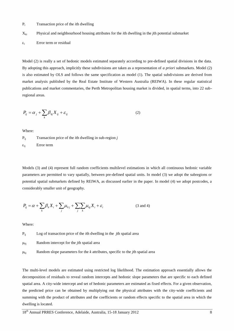
Model (2) is really a set of hedonic models estimated separately according to pre-defined spatial divisions in the data.

By adopting this approach, implicitly these subdivisions are taken as a representation of a priori submarkets. Model (2)

is also estimated by OLS and follows the same specification as model (1). The spatial subdivisions are derived from

market analysis published by the Real Estate Institute of Western Australia (REIWA). In these regular statistical

publications and market commentaries, the Perth Metropolitan housing market is divided, in spatial terms, into 22 sub-

regional areas.

k

ijijkjjij XP (2)

Where:

Pij Transaction price of the ith dwelling in sub-region j

ij Error term

Models (3) and (4) represent full random coefficients multilevel estimations in which all continuous hedonic variable

parameters are permitted to vary spatially, between pre-defined spatial units. In model (3) we adopt the subregions or

potential spatial submarkets defined by REIWA, as discussed earlier in the paper. In model (4) we adopt postcodes, a

considerably smaller unit of geography.

k j k

iikj

j

jikij XXP 0 (3 and 4)

Where:

Pij Log of transaction price of the ith dwelling in the jth spatial area

μ0j Random intercept for the jth spatial area

μkj Random slope parameters for the k attributes, specific to the jth spatial area

The multi-level models are estimated using restricted log likelihood. The estimation approach essentially allows the

decomposition of residuals to reveal random intercepts and hedonic slope parameters that are specific to each defined

spatial area. A city-wide intercept and set of hedonic parameters are estimated as fixed effects. For a given observation,

the predicted price can be obtained by multiplying out the physical attributes with the city-wide coefficients and

summing with the product of attributes and the coefficients or random effects specific to the spatial area in which the

dwelling is located.

18th


The estimations are carried out using a one year sample of housing transactions in the Perth metropolitan area, Western

Australia. A period extending from the middle of 2007 to the middle of 2008 was chosen as a study period after a

preliminary analysis (not reported in this paper) to determine a period of relative stability in the Perth metropolitan

housing market.

The hedonic data used for the estimations in this study were supplied on license by Landgate, the Western Australian

Land Information Authority. These data benefit from considerable detail in terms of hedonic attributes. There are

dummy variables describing the presence of ensuite and other bathrooms, dining, family, living and games rooms as

well as swimming pool and study or home office variables. Additional variables describe wall and roof construction,

location and property age. However, previous empirical work involving this particular dataset has highlighted

significant collinearity between many of these attribute variables and location. This is, of course, a common problem in

hedonic studies but it is particularly problematic in the context of this study since the main empirical objective is to

construct possible spatial submarkets from smaller geographical building blocks. The hedonic analyses therefore focus

on a reduced set of explanatory variables with descriptive statistics provided in table 1.

4. Estimation results

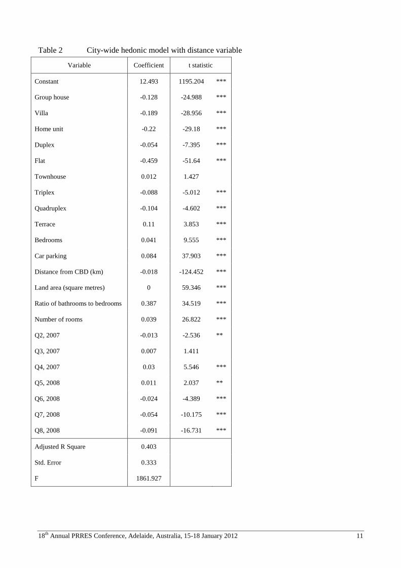
4.1 The benchmark model

The empirical performance of the city-wide hedonic model is, unsurprisingly, relatively poor. The adjusted R square is

0.40 (see table 2), although almost all of the physical attribute variables are statistically significant at the 1% level. The

‘house’ property type is implicit in the constant. Distance from the CBD is significant at 1% and negative, in line with

prior theoretical expectations. Despite the careful choice of a comparatively stable study period, the time dummy

variables indicate significant variation in transaction prices from the base period.

18th


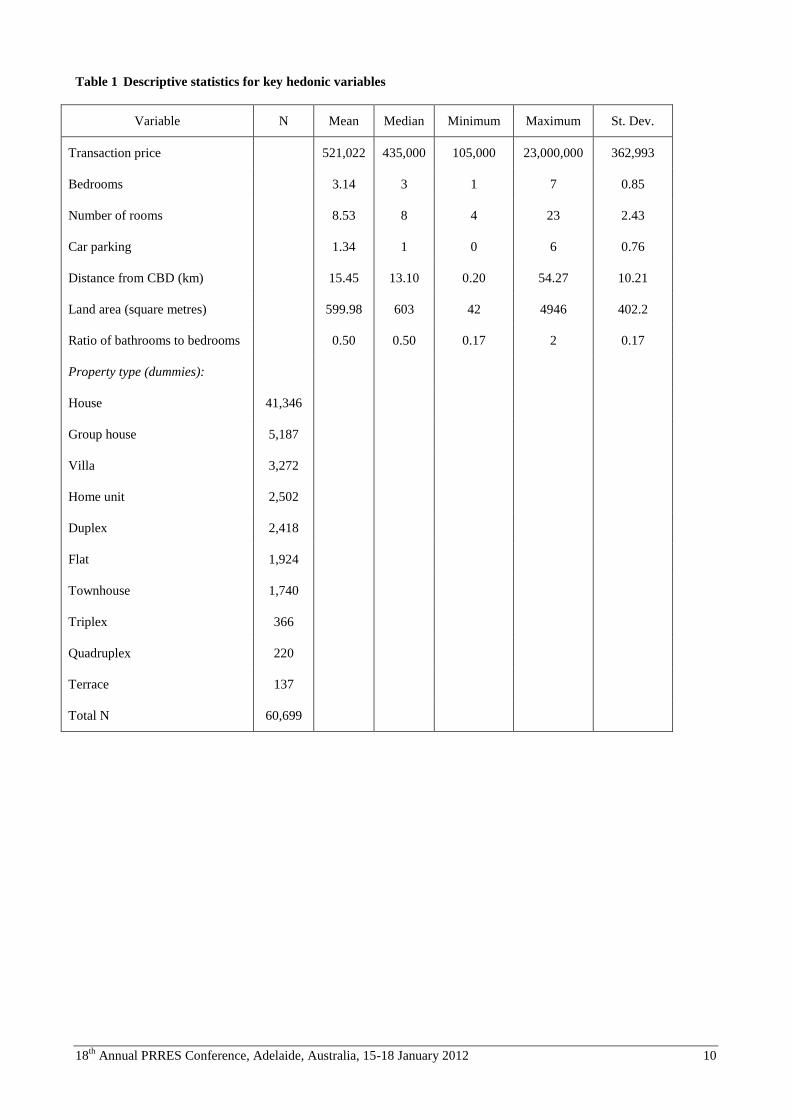
Table 1 Descriptive statistics for key hedonic variables

Variable N Mean Median Minimum Maximum St. Dev.

Transaction price 521,022 435,000 105,000 23,000,000 362,993

Bedrooms 3.14 3 1 7 0.85

Number of rooms 8.53 8 4 23 2.43

Car parking 1.34 1 0 6 0.76

Distance from CBD (km) 15.45 13.10 0.20 54.27 10.21

Land area (square metres) 599.98 603 42 4946 402.2

Ratio of bathrooms to bedrooms 0.50 0.50 0.17 2 0.17

Property type (dummies):

House 41,346

Group house 5,187

Villa 3,272

Home unit 2,502

Duplex 2,418

Flat 1,924

Townhouse 1,740

Triplex 366

Quadruplex 220

Terrace 137

Total N 60,699

18th


Table 2 City-wide hedonic model with distance variable

Variable Coefficient t statistic

Constant 12.493 1195.204 ***

Group house -0.128 -24.988 ***

Villa -0.189 -28.956 ***

Home unit -0.22 -29.18 ***

Duplex -0.054 -7.395 ***

Flat -0.459 -51.64 ***

Townhouse 0.012 1.427

Triplex -0.088 -5.012 ***

Quadruplex -0.104 -4.602 ***

Terrace 0.11 3.853 ***

Bedrooms 0.041 9.555 ***

Car parking 0.084 37.903 ***

Distance from CBD (km) -0.018 -124.452 ***

Land area (square metres) 0 59.346 ***

Ratio of bathrooms to bedrooms 0.387 34.519 ***

Number of rooms 0.039 26.822 ***

Q2, 2007 -0.013 -2.536 **

Q3, 2007 0.007 1.411

Q4, 2007 0.03 5.546 ***

Q5, 2008 0.011 2.037 **

Q6, 2008 -0.024 -4.389 ***

Q7, 2008 -0.054 -10.175 ***

Q8, 2008 -0.091 -16.731 ***

Adjusted R Square 0.403

Std. Error 0.333

F 1861.927

18th


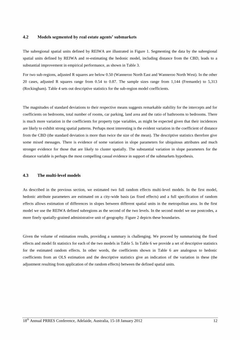
4.2 Models segmented by real estate agents’ submarkets

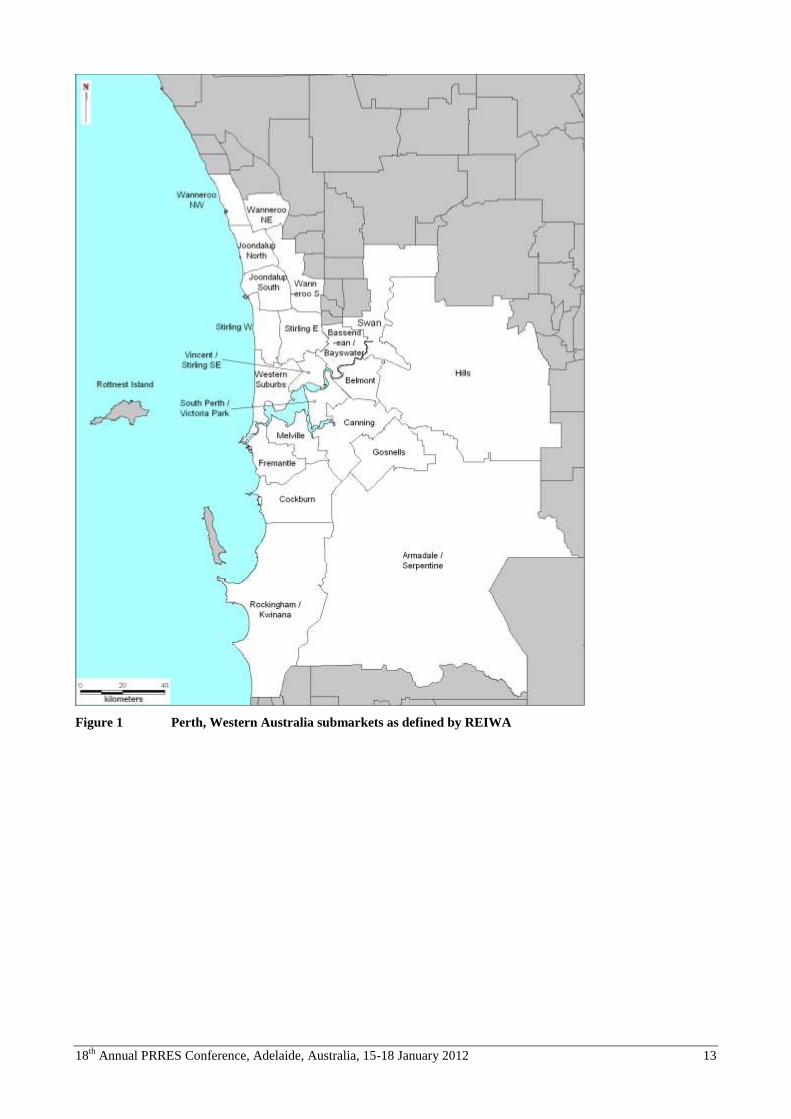
The subregional spatial units defined by REIWA are illustrated in Figure 1. Segmenting the data by the subregional

spatial units defined by REIWA and re-estimating the hedonic model, including distance from the CBD, leads to a

substantial improvement in empirical performance, as shown in Table 3.

For two sub-regions, adjusted R squares are below 0.50 (Wanneroo North East and Wanneroo North West). In the other

20 cases, adjusted R squares range from 0.54 to 0.87. The sample sizes range from 1,144 (Fremantle) to 5,313

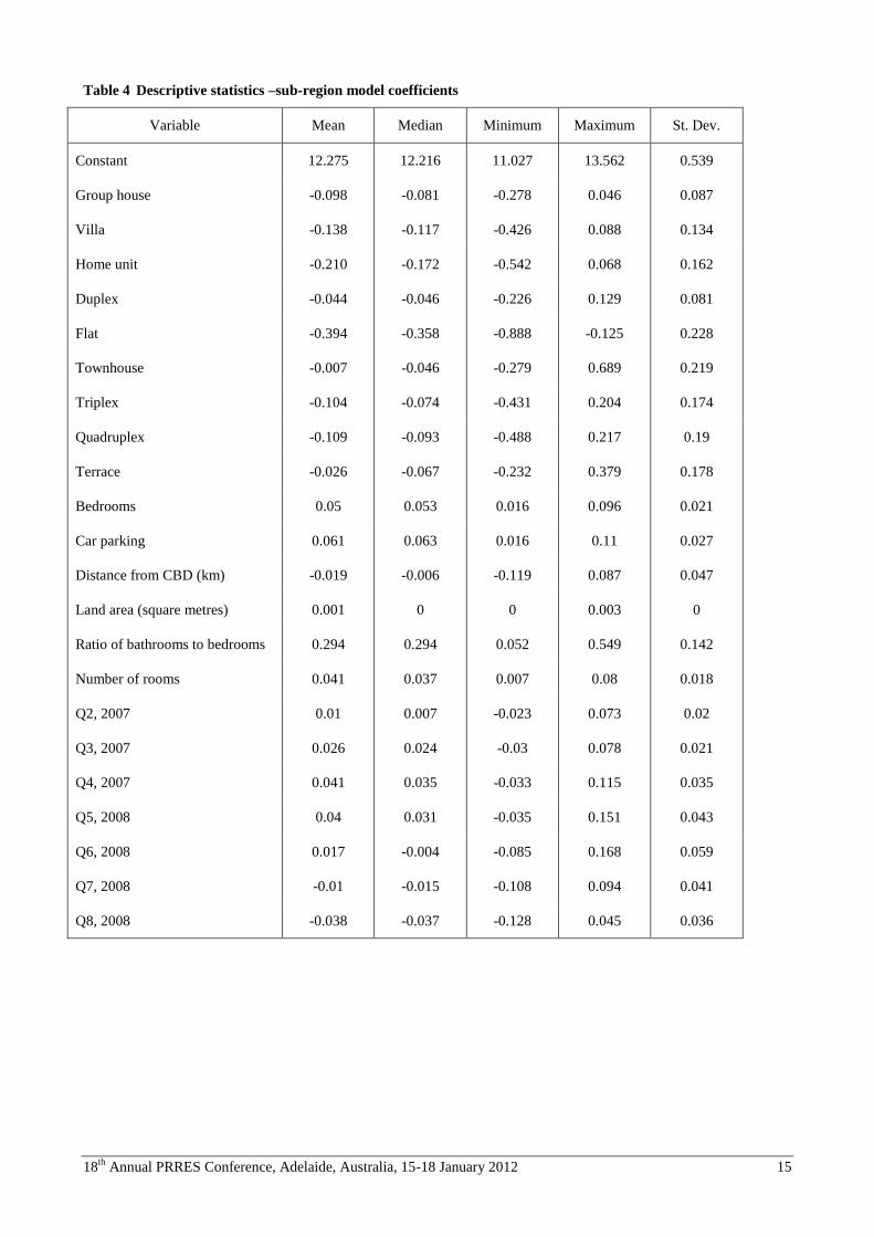
(Rockingham). Table 4 sets out descriptive statistics for the sub-region model coefficients.

The magnitudes of standard deviations to their respective means suggests remarkable stability for the intercepts and for

coefficients on bedrooms, total number of rooms, car parking, land area and the ratio of bathrooms to bedrooms. There

is much more variation in the coefficients for property type variables, as might be expected given that their incidences

are likely to exhibit strong spatial patterns. Perhaps most interesting is the evident variation in the coefficient of distance

from the CBD (the standard deviation is more than twice the size of the mean). The descriptive statistics therefore give

some mixed messages. There is evidence of some variation in slope parameters for ubiquitous attributes and much

stronger evidence for those that are likely to cluster spatially. The substantial variation in slope parameters for the

distance variable is perhaps the most compelling casual evidence in support of the submarkets hypothesis.

4.3 The multi-level models

As described in the previous section, we estimated two full random effects multi-level models. In the first model,

hedonic attribute parameters are estimated on a city-wide basis (as fixed effects) and a full specification of random

effects allows estimation of differences in slopes between different spatial units in the metropolitan area. In the first

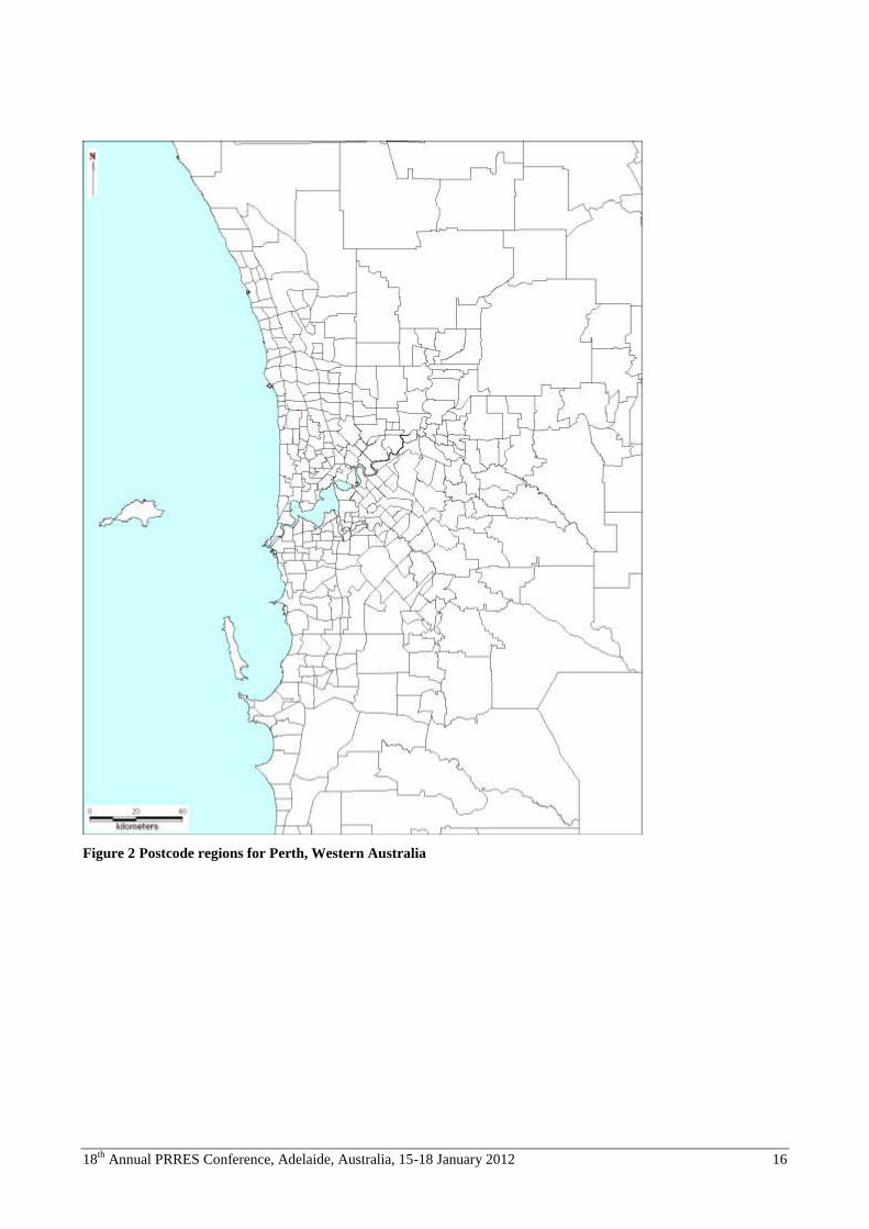
model we use the REIWA defined subregions as the second of the two levels. In the second model we use postcodes, a

more finely spatially-grained administrative unit of geography. Figure 2 depicts these boundaries.

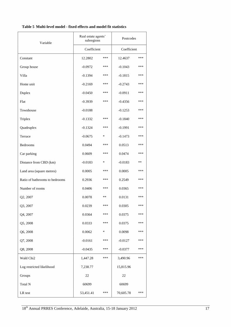
Given the volume of estimation results, providing a summary is challenging. We proceed by summarising the fixed

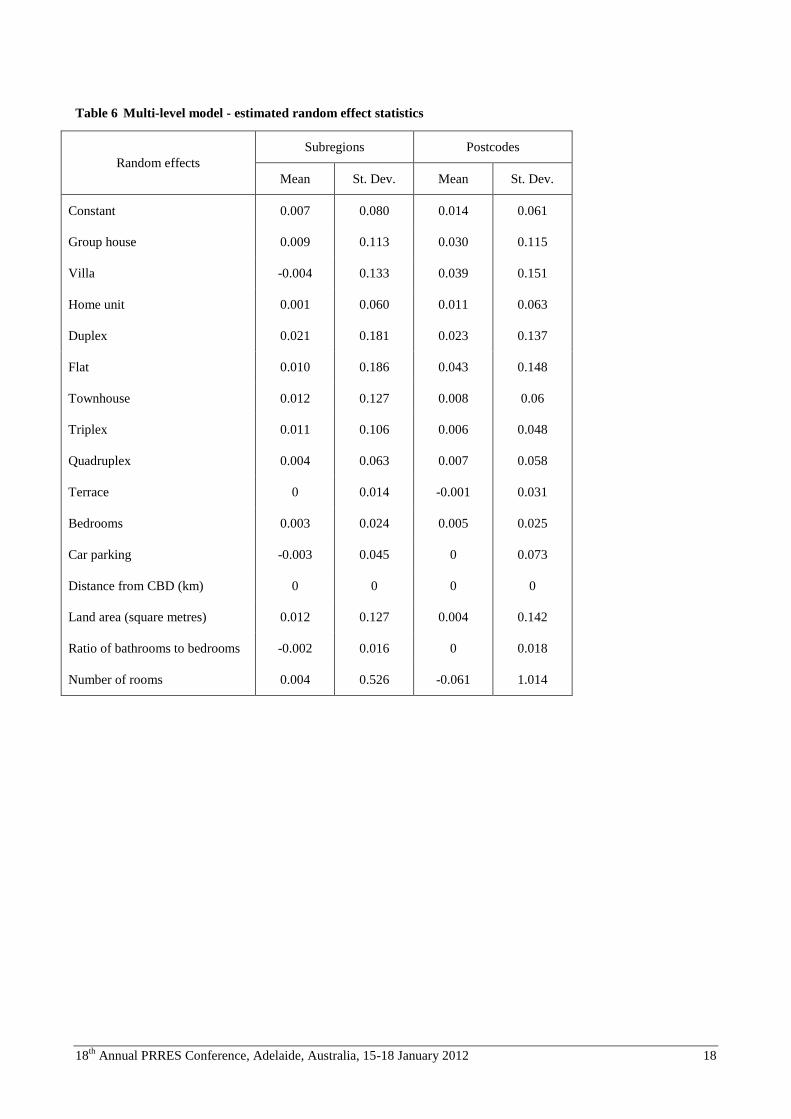
effects and model fit statistics for each of the two models in Table 5. In Table 6 we provide a set of descriptive statistics

for the estimated random effects. In other words, the coefficients shown in Table 6 are analogous to hedonic

coefficients from an OLS estimation and the descriptive statistics give an indication of the variation in these (the

adjustment resulting from application of the random effects) between the defined spatial units.

18th


Figure 1 Perth, Western Australia submarkets as defined by REIWA

18th


Table 3 Summary of sub-region hedonic models

Sub-region Adjusted R Square Std. Error of the Estimate

ARMADALE/SERPENTINE 0.646 0.184

BASSENDEAN/BAYSWATER 0.716 0.182

BELMONT 0.623 0.188

CANNING 0.544 0.193

COCKBURN 0.521 0.195

FREMANTLE 0.559 0.319

GOSNELLS 0.567 0.15

HILLS 0.566 0.195

JOONDALUP NORTH 0.504 0.226

JOONDALUP SOUTH 0.526 0.249

MELVILLE 0.686 0.25

PERTH CITY 0.742 0.209

ROCKINGHAM/KWINANA 0.518 0.207

SOUTH PERTH/VICTORIA PARK 0.723 0.242

STIRLING EAST 0.716 0.187

STIRLING WEST 0.666 0.235

SWAN 0.515 0.178

VINCENT/STIRLING SE 0.865 0.195

WANNEROO NORTH EAST 0.482 0.153

WANNEROO NORTH WEST 0.349 0.233

WANNEROO SOUTH 0.773 0.132

WESTERN SUBURBS 0.841 0.293

18th


Table 4 Descriptive statistics –sub-region model coefficients

Variable Mean Median Minimum Maximum St. Dev.

Constant 12.275 12.216 11.027 13.562 0.539

Group house -0.098 -0.081 -0.278 0.046 0.087

Villa -0.138 -0.117 -0.426 0.088 0.134

Home unit -0.210 -0.172 -0.542 0.068 0.162

Duplex -0.044 -0.046 -0.226 0.129 0.081

Flat -0.394 -0.358 -0.888 -0.125 0.228

Townhouse -0.007 -0.046 -0.279 0.689 0.219

Triplex -0.104 -0.074 -0.431 0.204 0.174

Quadruplex -0.109 -0.093 -0.488 0.217 0.19

Terrace -0.026 -0.067 -0.232 0.379 0.178

Bedrooms 0.05 0.053 0.016 0.096 0.021

Car parking 0.061 0.063 0.016 0.11 0.027

Distance from CBD (km) -0.019 -0.006 -0.119 0.087 0.047

Land area (square metres) 0.001 0 0 0.003 0

Ratio of bathrooms to bedrooms 0.294 0.294 0.052 0.549 0.142

Number of rooms 0.041 0.037 0.007 0.08 0.018

Q2, 2007 0.01 0.007 -0.023 0.073 0.02

Q3, 2007 0.026 0.024 -0.03 0.078 0.021

Q4, 2007 0.041 0.035 -0.033 0.115 0.035

Q5, 2008 0.04 0.031 -0.035 0.151 0.043

Q6, 2008 0.017 -0.004 -0.085 0.168 0.059

Q7, 2008 -0.01 -0.015 -0.108 0.094 0.041

Q8, 2008 -0.038 -0.037 -0.128 0.045 0.036

18th


Figure 2 Postcode regions for Perth, Western Australia

18th


Table 5 Multi-level model - fixed effects and model fit statistics

Variable

Real estate agents’

subregions Postcodes

Coefficient Coefficient

Constant 12.2802 *** 12.4637 ***

Group house -0.0972 *** -0.1043 ***

Villa -0.1394 *** -0.1815 ***

Home unit -0.2169 *** -0.2743 ***

Duplex -0.0450 *** -0.0911 ***

Flat -0.3939 *** -0.4356 ***

Townhouse -0.0188 -0.1253 ***

Triplex -0.1332 *** -0.1840 ***

Quadruplex -0.1324 *** -0.1991 ***

Terrace -0.0675 * -0.1473 ***

Bedrooms 0.0494 *** 0.0513 ***

Car parking 0.0609 *** 0.0474 ***

Distance from CBD (km) -0.0183 * -0.0183 **

Land area (square metres) 0.0005 *** 0.0005 ***

Ratio of bathrooms to bedrooms 0.2936 *** 0.2549 ***

Number of rooms 0.0406 *** 0.0365 ***

Q2, 2007 0.0078 ** 0.0131 ***

Q3, 2007 0.0239 *** 0.0305 ***

Q4, 2007 0.0364 *** 0.0375 ***

Q5, 2008 0.0333 *** 0.0375 ***

Q6, 2008 0.0062 * 0.0098 ***

Q7, 2008 -0.0161 *** -0.0127 ***

Q8, 2008 -0.0435 *** -0.0377 ***

Wald Chi2 1,447.28 *** 3,490.96 ***

Log restricted likelihood 7,238.77 15,815.96

Groups 22 22

Total N 60699 60699

LR test 53,451.41 *** 70,605.78 ***

18th


Table 6 Multi-level model - estimated random effect statistics

Random effects

Subregions Postcodes

Mean St. Dev. Mean St. Dev.

Constant 0.007 0.080 0.014 0.061

Group house 0.009 0.113 0.030 0.115

Villa -0.004 0.133 0.039 0.151

Home unit 0.001 0.060 0.011 0.063

Duplex 0.021 0.181 0.023 0.137

Flat 0.010 0.186 0.043 0.148

Townhouse 0.012 0.127 0.008 0.06

Triplex 0.011 0.106 0.006 0.048

Quadruplex 0.004 0.063 0.007 0.058

Terrace 0 0.014 -0.001 0.031

Bedrooms 0.003 0.024 0.005 0.025

Car parking -0.003 0.045 0 0.073

Distance from CBD (km) 0 0 0 0

Land area (square metres) 0.012 0.127 0.004 0.142

Ratio of bathrooms to bedrooms -0.002 0.016 0 0.018

Number of rooms 0.004 0.526 -0.061 1.014

18th


The ‘townhouse’ property type is not significant in the first multi-level model, but is significant at 1% in the second.

The ‘terrace’ property type variable is significant only at 10% in the first model, but is significant at 1% in the second.

The results are supportive of the idea that spatial aggregation in the presence of spatially varying attribute parameters

gives rise to misleading results. In the second model, the specification permits estimation of attribute parameters at a

much smaller scale. One of the benefits is that the city-wide parameter estimates appear to be more stable.

For most of the other variables, the results are generally stable between the two multi-level estimations. Differences in

parameter estimates seem to affect primarily the property type variables. Interestingly, the coefficient on distance from

the CBD is very stable between the two estimations. This result may appear surprising given its apparent instability in

the earlier hedonic estimations (models 1 and 2). In both cases the LR and Wald Chi square tests suggest strong

explanatory power, but at this stage little more can be said about the relative performance of models 3 and 4 given that

the likelihood ratios cannot be compared directly (since model 4 is specified with a greater number of random effects

parameters).

Given the impracticality of presenting coefficients for all defined spatial units, Table 6 summarises the mean and

standard deviation of the estimated random effects. As discussed in the previous section, these can be interpreted as

location-specific differences in attribute parameters (compared with the corresponding city-wide coefficients).

The descriptive statistics in Table 6 reveal instability in parameter estimates between the two estimation approaches. In

particular, in moving from a multi-level model with relatively large spatial units (REIWA sub-regions), to that with

smaller spatial units (postcodes) reveals:

The mean and standard deviation of the random effects differ noticeably for the ‘group house’, ‘villa’, ‘home

unit’ and ‘flat’ property type variables.

The mean random effect for ‘terrace’ is almost the same between the two estimations, but the standard

deviation is much larger in the finer spatially-grained model.

The mean random effects for bedrooms, car parking, the ratio of bathrooms to bedrooms and distance from the

CBD seem stable between the two models.

Random effects for land area and total number of rooms appear to have much more variation in the second

model than the first.

18th


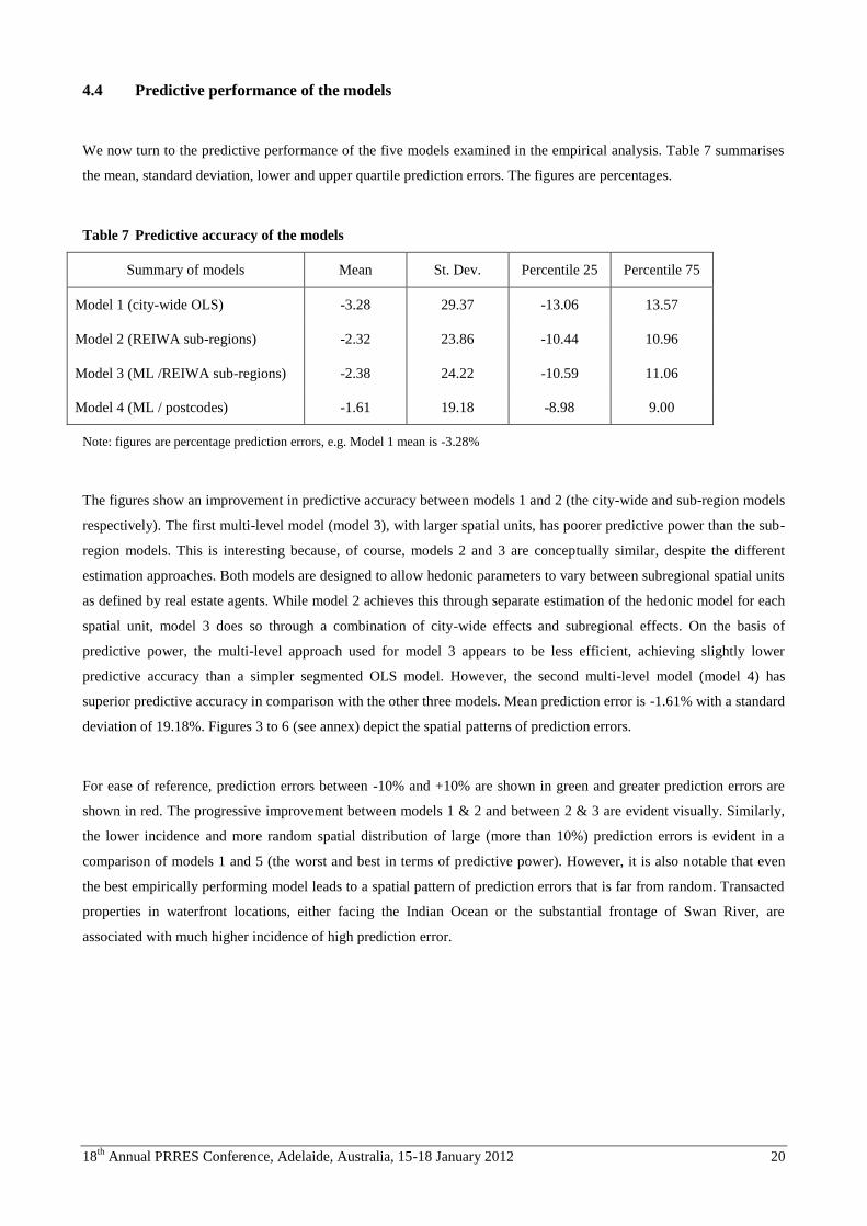
4.4 Predictive performance of the models

We now turn to the predictive performance of the five models examined in the empirical analysis. Table 7 summarises

the mean, standard deviation, lower and upper quartile prediction errors. The figures are percentages.

Table 7 Predictive accuracy of the models

Summary of models Mean St. Dev. Percentile 25 Percentile 75

Model 1 (city-wide OLS) -3.28 29.37 -13.06 13.57

Model 2 (REIWA sub-regions) -2.32 23.86 -10.44 10.96

Model 3 (ML /REIWA sub-regions) -2.38 24.22 -10.59 11.06

Model 4 (ML / postcodes) -1.61 19.18 -8.98 9.00

Note: figures are percentage prediction errors, e.g. Model 1 mean is -3.28%

The figures show an improvement in predictive accuracy between models 1 and 2 (the city-wide and sub-region models

respectively). The first multi-level model (model 3), with larger spatial units, has poorer predictive power than the sub-

region models. This is interesting because, of course, models 2 and 3 are conceptually similar, despite the different

estimation approaches. Both models are designed to allow hedonic parameters to vary between subregional spatial units

as defined by real estate agents. While model 2 achieves this through separate estimation of the hedonic model for each

spatial unit, model 3 does so through a combination of city-wide effects and subregional effects. On the basis of

predictive power, the multi-level approach used for model 3 appears to be less efficient, achieving slightly lower

predictive accuracy than a simpler segmented OLS model. However, the second multi-level model (model 4) has

superior predictive accuracy in comparison with the other three models. Mean prediction error is -1.61% with a standard

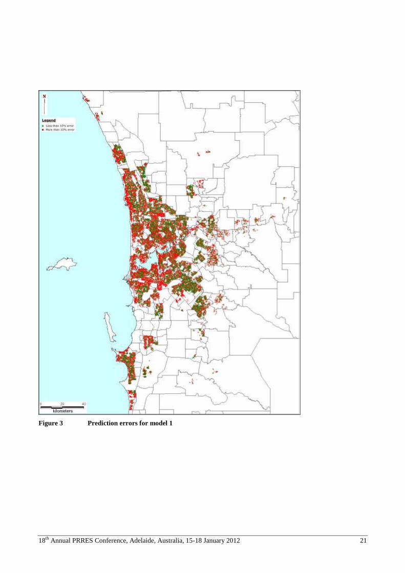
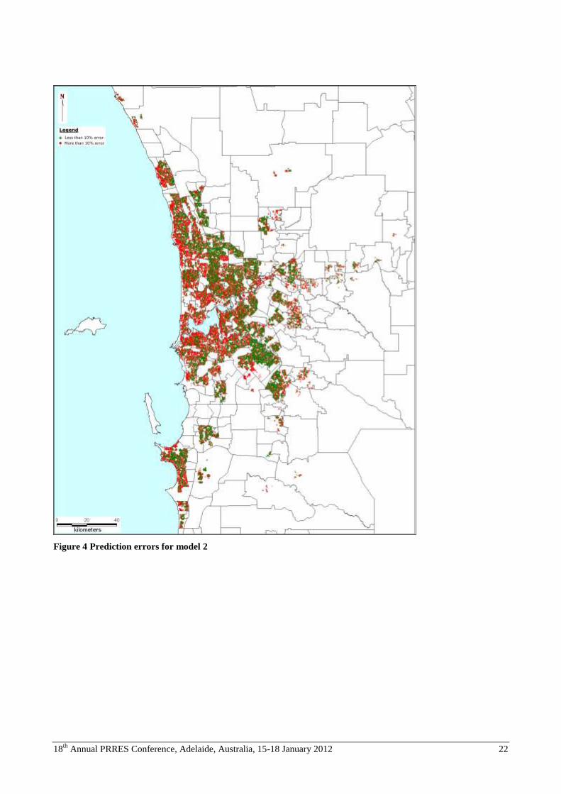
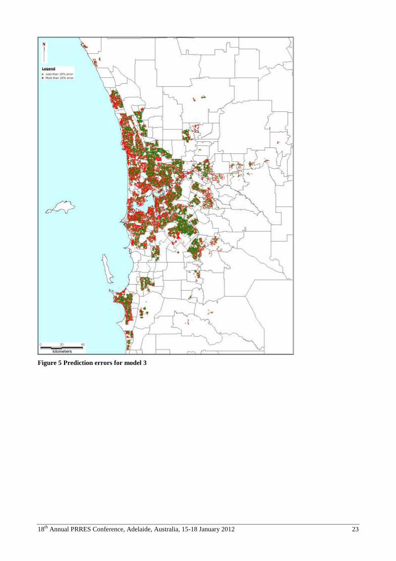
deviation of 19.18%. Figures 3 to 6 (see annex) depict the spatial patterns of prediction errors.

For ease of reference, prediction errors between -10% and +10% are shown in green and greater prediction errors are

shown in red. The progressive improvement between models 1 & 2 and between 2 & 3 are evident visually. Similarly,

the lower incidence and more random spatial distribution of large (more than 10%) prediction errors is evident in a

comparison of models 1 and 5 (the worst and best in terms of predictive power). However, it is also notable that even

the best empirically performing model leads to a spatial pattern of prediction errors that is far from random. Transacted

properties in waterfront locations, either facing the Indian Ocean or the substantial frontage of Swan River, are

associated with much higher incidence of high prediction error.

18th


Figure 3 Prediction errors for model 1

18th



18th


5 Conclusions

This paper set out to examine the utility of applying multi-level strategies to modelling spatial housing submarkets. The

empirical analysis was designed to compare the predictive performance of several models. Setting up a simple, city-

wide OLS hedonic model, with a simple distance variable, allowed us to establish a basic benchmark with which to

compare several alternative approaches. We found that separate estimation of the hedonic models for potential

submarkets (or subregions) defined by real estate agents led to a model that was superior to the benchmark in terms of

predictive power.

Estimation of multi-level hedonic models also led to improvement beyond the benchmark OLS model. Here however,

the predictive performance for one of the models (model 3) was slightly below that of the sub-region models on

average. This is an important and interesting finding in that it implies that a spatially segmented OLS estimation

approach is acceptable when there is certainty about spatial submarket boundaries, and would be appropriate when

submarket boundaries are expected to remain stable over time.

However, as we argue earlier, the best modelling strategy is not just that which produces the greatest predictive

accuracy. The best approach to modelling submarkets must also be able to capture the fluidity in submarket boundaries

over time. Where the spatial extent of submarket boundaries is less certain, or when there is an expectation of change in

these boundaries over time, our analysis suggests that a multi-level approach, with more finely spatially grained units of

geography, may be preferable to a segmented approach. Our second multi-level model (model 4), defined with smaller

spatial units, exhibits predictive performance that exceeded all other estimation approaches examined in this paper. The

spatial pattern of prediction errors is less concentrated. The results imply that multi-level models have the capacity to

improve predictive power and reduce spatial dependence when compared with standard hedonic methods. In addition,

when applied over time, multi-level models appear better able to deal with dynamic change in the composition of

submarkets and have the potential to capture the multiple (often nested) geographies that exist within local housing

systems. They can be used effectively to differentiate between neighbourhood, local (sub-regional) and regional

influences. More applied research is required, however, to exploit this potential.

18th


References

Adair, A.S., Berry, J. and McGreal, W.S. (1996) Hedonic modeling, housing submarkets, and residential valuation,

Journal of Property Research, 13, 1, 67-84

AUTHORS (2011) Evaluating agent-based definitions of housing submarkets in Perth, Working Paper (available on

request)

Ballas, D and Tranmer, M (2008) Happy places or happy people? A multi-level modelling approach to the analysis of

happiness and well-being, Mimeo, University of Sheffield

Ball, M. and Kirwan, R. (1977) Accessibility and supply constraints in the urban housing market, Urban Studies, 14,

11-32.

Bates, LK (2006) Does neighbourhood really matter? Comparing historically defined neighbourhood boundaries with

housing submarkets, Journal of Planning Education and Research, 26, 5-17

Berry, J, McGreal, S, Stevenson, S, Young, J and Webb, JR (2003) Estimation of apartment submarkets in Dublin,

Ireland, Journal of Real Estate Research, 25, 2, 159-170

Bourassa, S., Cantoni, E. and Hoesli, M. (2007) Spatial dependence, housing submarkets and house price prediction,

Journal of Real Estate Finance and Economics, Vol. 35, No. 2, 143-160.

Bourassa, S. Hamelink, F., Hoesli, M. and MacGregor, B.D. (1999) Defining housing submarkets, Journal of Housing

Economics, 8, 160-183

Bourassa, S., Hoesli, M. and Peng, V.S. (2003) Do housing submarkets really matter? Journal of Housing Economics,

Vol. 12, No. 1, 12-18.

Butler, R (1982) The specification of hedonic indexes for urban housing, Land Economics, 58, 96-102.

Can, A (1992) Specification and estimation of hedonic housing price models, Regional Science and Urban Economics,

22, 453-474

Clapp, JM and Wang, Y (2006) Defining neighborhood boundaries: are census tracts obsolete? Journal of Urban

Economics, 59, 259-284.

Costello, G, Leishman, C, Rowley, S and Watkins, C (2010) Modelling housing submarkets: comparing alternative

strategies, Paper presented to the ENHR Housing Economics Workshop, London

Fisher, E M and Fisher, R (1954) Urban Real Estate, New York, Henry Holt.

Fisher, E and Winnick, L (1952) The reformulation of the filtering concept, Journal of Social Issues, 7, 47-85.

18th


Fik, T., Ling, D. and Mulligan, G. (2003) Modeling spatial variation in housing prices: a variable interactions approach,

Real Estate Economics, 31, 4, 623-646.

Fletcher, M, Gallimore, P and Mangan, J (2000) The modeling of housing submarkets, Journal of Property Investment

and Finance, 4, 473-487

Galster, G (1996) William Grigsby and the analysis of housing submarkets and filtering, Urban Studies, 33, 10, 1797-

1806.

Galster, G and Rothenberg, J (1991) Filtering in a quality segmented model of urban housing markets, Journal of

Planning Education and Research, 11, 37-50.

Grigsby, WG (1963) Housing Markets and Public Policy, University of Pennsylvania Press, Philadelphia.

Goodman, AC (1978) Hedonic prices, price indices and housing markets, Journal of Urban Economics, 5, 471-484

Goodman, A.C. (1981) Housing submarkets within urban areas: definitions and evidence. Journal of Regional Science,

21, 175-185

Goodman, AC and Thibodeau, T (1998) Housing market segmentation, Journal of Housing Economics, 7, 121-143.

Goodman, AC and Thibodeau, T (2003) Housing market segmentation and hedonic prediction accuracy, Journal of

Housing Economics, 12, 181-201.

Goodman, AC and Thibodeau, T (2007) The spatial proximity of metropolitan housing submarkets, Real Estate

Economics, 35, 209-232.

Jones, C, Leishman, C and Watkins, C (2003) Structural change in a local urban housing markets, Environment and

Planning A, 34, 1315-1326.

Jones, C, Leishman, C. and Watkins, C. (2004) Intra-urban migration and housing submarkets: theory and evidence,

Housing Studies, Vol. 19, No. 2, 269-283.

Jones, K and Bullen, N (1993) A multilevel analysis of the variation in domestic property prices: southern England

1980-1987, Urban Studies, 30, 8, 1409-1426

Jones, K and Bullen, N (1994) Contextual models of urban house prices: a comparison of fixed – and random –

coefficient models developed by expansion, Economic Geography, 70, 3, 252-272

Keskin, B (2010) Alternative Approaches to Modelling Housing Submarkets: Evidence from Istanbul, Unpublished PhD

Thesis, University of Sheffield, Sheffield.

Kauko, T, Hakfoort, J and Hooimeijer, P (2002) Capturing housing market segmentation: an alternative approach based

on neural network modeling, Housing Studies, 17, 875-894

18th


Leishman, C. (2009) Spatial change and the structure of urban housing sub-markets, Housing Studies, Vol. 24, No. 5,

563-585.

Maclennan, D, (1982) Housing Economics, Longman.

Maclennan, D, Munro, M and Wood, G (1987) Housing choice and the structure of urban housing

markets, in Turner, B, Kemeny, J and Lundquist, L (Eds) Between State and Market Housing in the

Post-Industrial Era, Almquist and Hicksell, Gothenburg.

Maclennan, D. and Tu, Y. (1996) Economic perspectives on the structure of local housing markets, Housing Studies,

Vol. 11, No. 3, 387-406

McGreal, WS, Adair, AS, Smyth, A, Cooper, J and Ryley, T (2000) House prices and accessibility: the testing of

relationships within the Belfast area, Housing Studies, 15, 699-716

Michaels, R and Smith, VK (1990) Market segmentation and valuing amenities with hedonic models: the case of

hazardous waste sites, Journal of Urban Economics, 28, 223-242.

Moon, G, Subramanian, SV, Jones, K, Duncan, C and Twigg, L (2005) Area-based studies and the evaluation of

multilevel influences on health outcomes, in Bowling, A and Ebrahim, S (ed) Handbook of Health Research Methods,

Open Uni Press, Berkshire.

Orford, S (1999) Valuing the Built Environment: GIS and House Price Analysis, Ashgate, Aldershot

Orford, S (2000) Modelling spatial structures in local housing market dynamics: a multilevel perspective, Urban

Studies, 37, 1643-1670

Orford, S (2002) Valuing locational externalities: a GIS and multilevel modelling approach, Environment and Planning

B: Planning and Design, 29, 105-127

Palm, R (1978) Spatial segmentation of the urban housing market, Economic Geography, 54, 210-21

Pavlov, A.D. (2000) Space-varying regression coefficients: a semi-parametric approach applied to real estate markets,

Real Estate Economics, 28, 2, 249-283.

Rothenberg, J, Galster, G, Butler, R and Pitkin, J (1991) The Maze of Urban Housing Markets: Theory, Evidence and

Policy, University of Chicago Press, Chicago.

Schnare, A and Struyk, R (1976) Segmentation in urban housing markets, Journal of Urban Economics, 3, 146-166.

Spinney, J, Kanaroglou, P and Scott, D (2011) Exploring spatial dynamics and land price indexes, Urban Studies, 46,

719-734

Straszheim, M. (1975) An Econometric Analysis of the Urban Housing Market, National Bureau of Economic Research,

New York

18th


Subramanian, SV (2010) Multilevel modelling, in Fischer, MM and Getis, A (eds) Handbook of Spatial Analysis:

Software, Tools, Methods and Applications, Spriner-Verlag, Berlin

Tu, Y., Sun, H. and Yu, S-M. (2007) Spatial autocorrelation and urban housing market segmentation, Journal of Real

Estate Finance and Economics, 34, 385-406.

Watkins, C (2001) The definition and identification of housing submarkets, Environment and Planning A, 33, 2235-

2253.

Watkins, C (2008) Microeconomic perspectives on the structure and operation of local housing markets, Housing

Studies, 23,163-178

Watkins, C (2011) Housing Submarkets, in International Encyclopaedia of Housing and Home, Smith, S (Ed), in press

18th annual pacific-rim real estate society … · this paper seeks to move the focus on to the...

Documents