1982 ieee transactions on knowledge and data...

Approximate Algorithms for Computing SpatialDistance Histograms with Accuracy Guarantees

Vladimir Grupcev, Student Member, IEEE, Yongke Yuan, Yi-Cheng Tu, Member, IEEE,

Jin Huang, Student Member, IEEE, Shaoping Chen, Sagar Pandit, and Michael Weng

Abstract—Particle simulation has become an important research tool in many scientific and engineering fields. Data generated by

such simulations impose great challenges to database storage and query processing. One of the queries against particle simulation

data, the spatial distance histogram (SDH) query, is the building block of many high-level analytics, and requires quadratic time to

compute using a straightforward algorithm. Previous work has developed efficient algorithms that compute exact SDHs. While beating

the naive solution, such algorithms are still not practical in processing SDH queries against large-scale simulation data. In this paper,

we take a different path to tackle this problem by focusing on approximate algorithms with provable error bounds. We first present a

solution derived from the aforementioned exact SDH algorithm, and this solution has running time that is unrelated to the system size

N. We also develop a mathematical model to analyze the mechanism that leads to errors in the basic approximate algorithm. Our

model provides insights on how the algorithm can be improved to achieve higher accuracy and efficiency. Such insights give rise to a

new approximate algorithm with improved time/accuracy tradeoff. Experimental results confirm our analysis.

Index Terms—Molecular simulation, spatial distance histogram, quadtree, scientific databases

Ç

1 INTRODUCTION

MANY scientific fields have undergone a transition todata/computation intensive science, as the result of

automated experimental equipments and computer simula-tions. In recent years, much progress has been made inbuilding data management tools suitable for processingscientific data [1], [2], [3], [4], [5]. Scientific data imposegreat challenges to the design of database managementsystems that are traditionally optimized toward handlingbusiness applications. First, scientific data often come inlarge volumes that require us to rethink the storage,retrieval, and replication techniques in current DBMSs.Second, user accesses to scientific databases are focused oncomplex high-level analytics and reasoning that go beyondsimple aggregate queries. While many types of domain-specific analytical queries are seen in scientific databases,the DBMS should support efficient processing of those that

are frequently used as building blocks for more complexanalysis. However, many of such basic analytical queriesneed superlinear processing time if handled in a straight-forward way, as in current scientific databases. In thispaper, we report our efforts to design efficient algorithmsfor a type of query that is extremely important in theanalysis of particle simulation data.

Particle simulations are computer simulations in whichthe basic components (e.g., atoms, stars, etc.) of largesystems (e.g., molecules, galaxies, etc.) are treated asclassical entities that interact for certain duration underpostulated empirical forces. For example, molecular simu-lations (MSs) explore relationship between molecularstructure, movement, and function. These techniques areprimarily applicable in modeling of complex chemical andbiological systems that are beyond the scope of theoreticalmodels. MS has become an important research tool inmaterial sciences [6], astrophysics [7], biomedical sciences,and biophysics [8], motivated by a wide range ofapplications. In astrophysics, the N-body simulations arepredominantly used to describe large scale celestialstructure formation [8], [9], [10], [11]. Similar to MS inapplicability and simulation techniques, the N-body simu-lation comes with even larger scales in terms of totalnumber of particles simulated.

Results of particle simulations form large data sets ofparticle configurations. Typically, these configurations storeinformation about the particle types, their coordinates, andvelocities—the same type of data we have seen in spatial-temporal databases [12]. While snapshots of configurationsare interesting, quantitative structural analysis of intera-tomic structures are the mainstream tasks in data analysis.This requires the calculation of statistical properties orfunctions of particle coordinates [9]. Of special interest toscientists are those quantities that require coordinates of

1982 IEEE TRANSACTIONS ON KNOWLEDGE AND DATA ENGINEERING, VOL. 25, NO. 9, SEPTEMBER 2013

. V. Grupcev and Y.-C. Tu are with the Department of Computer Scienceand Engineering, University of South Florida, 4202 E. Fowler Ave., ENB118, Tampa, FL 33620. E-mail: [email protected], [email protected].

. Y. Yuan and M. Weng are with the Department of Industrial andManagement Systems Engineering, University of South Florida,4202 E. Fowler Ave., ENB118, Tampa, FL 33620.E-mail: {yyuan, mxweng}@usf.edu.

. J. Huang is with the Department of Computer Science, University of Texasat Arlington, 500 UTA Boulevard, Room 640, ERB Buildings, Arlington,TX 76019. E-mail: [email protected].

. S. Chen is with the Department of Mathematics, Wuhan University ofTechnology, 122 Luosi Road, Wuhan, Hubei 430070, P.R. China.E-mail: [email protected].

. S. Pandit is with the Department of Physics, University of South Florida,4202 E. Fowler Ave., PHY114, Tampa, FL 33620.E-mail: [email protected].

Manuscript received 18 Oct. 2011; revised 16 Apr. 2012; accepted 12 July2012; published online 25 July 2012.Recommended for acceptance by C. Shahabi.For information on obtaining reprints of this article, please send e-mail to:[email protected], and reference IEEECS Log Number TKDE-2011-10-0639.Digital Object Identifier no. 10.1109/TKDE.2012.149.

1041-4347/13/$31.00 � 2013 IEEE Published by the IEEE Computer Society

two particles simultaneously. In their brute-force form,these quantities require OðN2Þ computations for N particles[8]. In this paper, we focus on one such analytical query: theSpatial Distance Histogram (SDH) query, which asks for ahistogram of the distances of all pairs of particles in thesimulated system.

1.1 Problem Statement

The problem can be defined as follows: given thecoordinates of N points in space, we are to compute thecounts of point-to-point distances that fall into a series ofl ranges in the IR domain: ½r0; r1Þ; ½r1; r2Þ; ½r2; r3Þ; . . . ; ½rl�1; rl�.A range ½ri; riþ1Þ in such series is called a bucket, and thespan of the range riþ1 � ri is called the width of the bucket.In this paper, we focus our discussions on the case ofstandard SDH queries, where all buckets have the same widthp and r0 ¼ 0, which gives the following series of buckets:½0; pÞ; ½p; 2pÞ; . . . ; ½ðl� 1Þp; lp�. Generally, the boundary of thelast bucket lp is set to be the maximum distance of any pairof points in the data set. Although almost all scientific dataanalysis only require the computation of standard SDHqueries, our solutions can be easily extended to handlehistograms with nonuniform bucket width and/or arbitraryvalues of r0 and rl.

1 The answer to an SDH query isbasically a series of nonnegative integers h ¼ ðh1; h2; . . . ; hlÞ,where hi ð0 < i � lÞ is the number of pairs of points whosedistances are within the bucket ½ði� 1Þp; ipÞ.

1.2 Motivation

The SDH is a fundamental tool in the validation andanalysis of particle simulation data. It serves as the mainbuilding block of a series of critical quantities to describe aphysical system. Specifically, SDH is a direct estimation of acontinuous statistical distribution function called radialdistribution functions (RDF) [7], [9], [13] that is defined as

gðrÞ ¼ NðrÞ4�r2�r�

; ð1Þ

where NðrÞ is the expected number of atoms in the shellbetween r and rþ �r around any particle, � is the averagedensity of particles in the whole system, and 4�r2�r is thevolume of the shell. Since SDH directly provides the valuefor NðrÞ, the RDF can be viewed as a normalized SDH.

The RDF is of great importance in computation ofthermodynamic quantities about the simulated system.Some of the important quantities like total pressure,

p ¼ �kT � 2�

3�2

Zdrr3u0ðrÞgðr; �; T Þ;

and energy,

E

NkT¼ 3

2þ �

2kT

Zdr 4�r2uðrÞgðr; �; T Þ;

can be derived in terms of structure factor that can beexpressed using gðrÞ [14]. For monoatomic systems, therelation between RDF and the structure factor of the system[15] takes simple form, viz.,

SðkÞ ¼ 1þ 4��

k

Z 10

gðrÞ � 1ð Þr sinðkrÞ dr:

The definitions of all notations in the above formulas canbe found in [14] and [15]. To compute SDH in astraightforward way, we have to calculate distancesbetween all pairs of particles and put the distances intobins with a user-specified width, as done in state-of-the-artsimulation data analysis software packages [7], [16]. MS orN-body techniques generally consist of large number ofparticles. For example, the Virgo consortium has accom-plished a simulation containing 10 billion particles to studythe formation of galaxies and quasars [17]. This kind ofscale prohibits the analysis of large data sets following thebrute-force approach. From a database viewpoint, it wouldbe desirable to make SDH a basic query type with thesupport of scalable algorithms.

Previous work [18], [19] have addressed this problem bydeveloping algorithms that compute exact SDHs with timecomplexity lower than quadratic. The main idea is toorganize the data in a space-partitioning tree and processpairs of tree nodes instead of pairs of particles (thus savingprocessing time). The tree structure used include kd-tree in[18] and region quad/oct-tree in our previous work [19],which also proved that the time complexity of suchalgorithms is OðN 2d�1

d Þ, where d 2 f2; 3g is the number ofdimensions in the data space. While beating the naivesolution in performance, such algorithms’ running time forlarge data sets can still be undesirably long. On the otherhand, an SDH with some bounded error can satisfy theneeds of users. In fact, there are cases where even a coarseSDH will greatly help the fine-tuning of simulationprograms [9]. Generally speaking, the main motivation toprocess SDHs is to study the statistical distribution of point-to-point distances in the simulated system [9]. Since ahistogram by itself is an approximation of the underlyingdistribution gðrÞ (1), an inaccurate histogram generatedfrom a given data set will still be useful in a statistical sense.Therefore, in this paper, we focus on approximate algo-rithms with very high performance that deliver queryresults with low error rates. In addition to experimentalresults, we also evaluate the performance/accuracy trade-offs provided by the proposed algorithms in an analyticalway. The running time of our proposed algorithm is onlyrelated to the desired accuracy. Our experimental resultsshow significant improvement in performance/accuracytradeoff of our algorithm over the previous algorithms—theerror rates in query results are very small even when therunning time is reasonably short.

1.3 Roadmap of the Paper

We continue this paper by a survey of related work and alist of our contributions in Section 2; we introduce thetechnical background on which our approximate algorithmis built in Section 3; we describe the details of a basicapproximate algorithm and relevant empirical evaluation inSection 4; we dedicate Section 6 to mathematical analysis ofthe key mechanisms in our basic algorithm; the results ofour analytical work are used to develop a new algorithmwith improved performance and we introduce and evaluatethat algorithm in Section 7; Section 8 concludes this paper.

GRUPCEV ET AL.: APPROXIMATE ALGORITHMS FOR COMPUTING SPATIAL DISTANCE HISTOGRAMS WITH ACCURACY GUARANTEES 1983

1. The only complication of nonuniform bucket width is that, given adistance value, we need Oðlog lÞ time to locate the bucket instead of constanttime for equal bucket width.

2 RELATED WORK AND OUR CONTRIBUTIONS

The scientific community has gradually moved fromprocessing large data files toward using database systemsfor the storage, retrieval, and analysis of large-scalescientific data [2], [20]. Conventional (relational) databasesystems are designed and optimized toward data andapplications from the business world. In recent years, thedatabase community has invested much efforts into con-structing database systems that are suitable for handlingscientific data. For example, the BDBMS project [3] handlesannotation and provenance of biological sequence data; andthe PeriScope [5] project is aimed at efficient processing ofdeclarative queries against biological sequences. In additionto that, there are also proposals of new DBMS architecturesfor scientific data management [21], [22], [23]. The mainchallenges and possible solutions of scientific data manage-ment are discussed in [1].

Traditionally, MS data are stored in large files andqueries are implemented in stand-alone programs, asrepresented by popular simulation/analytics packages[16]. Recent efforts have been dedicated to buildingsimulation data management systems on top of relationaldatabases, as represented by the BioSimGrid [4] and SimDB[24] projects developed for MSs. However, such systems arestill in short of efficient query processing strategies. To thebest of our knowledge, the computation of SDH in suchsoftware packages is done in a brute-force way, whichrequires OðN2Þ time.

In particle simulations, the computation of (gravita-tional/electrostatic) force is similar to the SDH problem.Specifically, the force is the sum of all pairwise interactionsin the system, thus requires OðN2Þ steps to compute. Thesimulation community has adopted approximate solutionsrepresented by the Barnes-Hut algorithm that runs onOðN logNÞ time [25] and the Multipole algorithm [26] withlinear running time. Although all above algorithms use atree-like data structure to hold the data, they provide littleinsights on how to solve the SDH problem. The mainreason is that these strategies take advantage of twofeatures of force: 1) for any pairwise interaction, itscontribution to the force decreases dramatically whenparticle distance increases; 2) the effects of symmetricinteractions cancel out. However, neither features areapplicable to SDH computation, in which every pairwiseinteraction counts and all are equally important. Anothermethod for force computation is based on well-separatedpair decomposition (WSPD) [27] and was found to beequivalent to the Barnes-Hut algorithm. A WSPD is acollection of pairs of subsets of the data such that all point-to-point distances are covered by such pairs. The pairs ofsubsets are also well separated in that the smallest distancebetween the smallest balls covering the subsets (with radiusr) is at least sr, where s is a user-defined parameter.Although relevant by intuition, the WSPD does not producefast solution for SDH computation.

It is worth mentioning that there has been work done ona broader problem of histogram computation in the contextof data stream management [28]. The data stream systemsusually work with distributive aggregates [28] such asCOUNT, SUM, MAX, and MIN which may be computed

incrementally using constant space and time. They alsotackle so called holistic aggregates such as TOP-k [29], [30],QUANTILE [31], and COUNT DISTINCT [32], [33]. Whencomputing the holistic aggregates they have utilized hash-based functions that produce histograms [30], [34]. But thedata stream community has never specifically worked onthe problem of computing a histogram that will disclose thedistance counts belonging to a particular range (a bucket),i.e., an SDH. After thoroughly reviewing their work, webelieve that none of their proposed solutions is directlyapplicable to the problem of SDH computation stated inthis paper.

Another similar problem to the SDH computation is tofind k-nearest neighbors (kNN) in a high-dimensional space[35]. In such a problem, avoidance of distance computationis the primary goal in algorithmic design due to the highcost of such operations. The main technique is to choose aset of reference points (i.e., pivots) in the database andprecompute distances between data points to the pivots. Inprocessing kNN queries, the search space can be prunedbased on the precomputed distances. However, being asearching problem, kNN is very different from the count-ing-based SDH problem. As a result, the data structures andalgorithmic details shown in [35] have little overlap withour solutions to the SDH problem.

Although SDH is an important analytics, there is notmuch elaboration on efficient SDH algorithms. An earlierwork from the data mining community [18] opened thedirection of processing SDHs by space-partitioning trees.The core idea is to process all the particles in a tree node asone single entity to take advantage of the nonzero bucketwidth p. By this, processing time is saved by avoidingcomputation of particle-to-particle distances. Our earlierpaper [19] proposed a similar algorithm as well as rigorousmathematical analysis (not found in [18]) of the algorithm’stime complexity. Specifically, in [19], we proposed a novelalgorithm (named DM-SDH) to compute SDH based on adata structure called density map, which can be easilyimplemented by augmenting a Quadtree index. Contrary tothat, the data structure adapted in [18] is the kd-tree. Ourmathematical analysis [36] has shown that the algorithmruns on �ðN 3

2Þ for two-dimensional data and �ðN 53Þ for

three-dimensional data, respectively. The technical detailsof such an algorithm will be introduced in Section 3.

This paper significantly extends our earlier work [19]by focusing on approximate algorithms for SDH proces-sing. In particular, we claim the following contributionsvia this work:

1. We present an approximate SDH processing strategythat is derived from the basic exact algorithm, andthis approximate algorithm has constant-time com-plexity and a provable error bound;

2. We develop a mathematical model to analyze theeffects of error compensation that led to highaccuracy of our algorithm; and

3. We propose an improved approximate algorithmbased on the insights obtained from the aboveanalytical results.

It is also worth mentioning that we have recentlypublished another paper [37] in this field. That paper


focuses on a more sophisticated heuristics to generateapproximate results based on spatial uniformity of dataitems. Such heuristics improves the accuracy of eachdistance distribution, which is the basic operation of ourapproximate algorithm (Section 4.1). In this paper, weintroduce the design of the approximate algorithm and itsperformance analysis. Technically, we emphasize theimpacts of error compensation among different distributionoperations. As a result, we do not require low error rates tobe obtained from each operation, as we show the total erroris low even when a primitive heuristics is used. In otherwords, these two papers, although both take approximateSDH processing as the basic theme, make their contribu-tions at two different levels of the problem. Work in [37]focuses on improving accuracy of single distributionoperations while this paper, in addition to a systematicdescription of the algorithm, studies how errors fromdifferent distribution operations cancel out each other,and to what extent such error compensation affects theaccuracy of the final results.

3 PRELIMINARIES

In this section, we introduce the algorithm we developed in[19] to compute exact SDHs. Techniques and analysisrelated to this algorithm are the basis for the approximatealgorithm we focus on in this paper. In Table 1, we list thenotations that are used throughout this paper. Note thatsymbols defined and referenced in a local context are notlisted here.

3.1 Overview of the Density Map-Based SDH(DM-SDH) Algorithm

To beat the OðN2Þ time needed by the naive solution, weneed to avoid the computation of all particle-to-particledistances. An important observation here is: a histogrambucket always has a nonzero width p. Given a pair of points,their bucket membership could be determined if we onlyknow a range that the distance belongs to and this range iscontained in a histogram bucket. The central idea of ourapproach is a data structure called density map, which isbasically a grid containing cells of equal size.2 In every cellof the grid, we record the number of particles that arelocated in the space represented by that cell as well as the

four coordinates that determine the exact boundary of thecell in space. The reciprocal of the cell size in a density mapis called the resolution of the density map. To process theSDH query, we build a series of density maps with differentresolutions. We organize all such density maps into a pointregion (PR) Quadtree [38], in which the resolution of adensity map (i.e., all nodes on level i of the tree) is alwaysdoubled as compared to the previous one (i.e., those onlevel i� 1) in the series.

The pseudocode of the DM-SDH algorithm can be foundin Fig. 1. The core of the algorithm is a procedure namedRESOLVETWOCELLS, which is given as input a pair of cellsM1 and M2 on the same density map. In RESOLVETWO-

CELLS, we first compute the minimum and maximumdistances between any particle from M1 and any one fromM2 (line 1). Obviously, this can be accomplished in constanttime given the corner coordinates of two cells stored in thedensity map. When the minimum and maximum distancesbetween M1 and M2 fall into the same histogram bucket i,we say these two cells are resolvable on this density map,and they resolve into bucket i. If this happens, the histogramis updated (lines 2-5) by incrementing the count of thespecific bucket i by n1n2, where n1; n2 are the particle countsin cells M1 and M2, respectively. If the two cells do notresolve on the current density map, we move to a densitymap with higher (doubled) resolution and repeat theprevious step. However, on this new density map, we tryresolving all four partitions of M1 with all those of M2

(lines 12-16). In other words, there are 4� 4 ¼ 16 recursivecalls to RESOLVETWOCELLS if M1 and M2 are not resolvable


TABLE 1Symbols and Notations

Fig. 1. The DM-SDH algorithm.

2. From now on, we use 2D data and grids to elaborate our ideas unlessspecified otherwise. Note that extending our discussions to 3D data/spacewould be straightforward, as studied in [36].

on the current density map. In another scenario, where M1

and M2 are not resolvable yet no more density maps areavailable, we have to calculate the distances of all particlesin the nonresolvable cells (lines 6-11). The DM-SDHalgorithm starts at the first density map DMo whose celldiagonal length is smaller than the histogram bucket widthp (line 2). It is easy to see that no pairs of cells are resolvablein density maps with resolution lower than that of DMo.Within each cell on DMo, we are sure that any intracellpoint-to-point distance is smaller than p; thus, all suchdistances are counted into the first bucket with range ½0; pÞ(lines 3-5). The algorithm proceeds by resolving intercelldistances (i.e., calling RESOLVETWOCELLS) for all pairs ofcells in DMo (lines 6-7).

In DM-SDH, an important implementation detail that isrelevant to our approximate algorithm design is the heightof the quadtree (i.e., the number of density map levels).Recall that DM-SDH saves time by resolving cells such thatwe need not to calculate the point-to-point distances one byone. However, when the total point counts in a celldecreases, the time we save by resolving that cell alsodecreases. Imagine a cell with only four or fewer (eight for3D data/space) data points; it does not give us any benefitin SDH query processing to further partition this cell on thenext level: the cost of resolving the partitions could behigher than directly retrieving the particles and calculatingdistances (lines 7-11 in RESOLVETWOCELLS). Based on thisobservation, the total level of density maps H is set to be

H ¼�

log2dN

�

�þ 1; ð2Þ

where d is the number of dimensions, 2d is the degree of thenodes in the tree (4/8 for 2D/3D data), and � is the averagenumber of particles we desire in each leaf node. In practice,we set � to be slightly greater than 4 in 2D (8 for 3D data)because the CPU cost of resolving two cells is higher thancomputing the distance between two points.

3.2 Performance Analysis of DM-SDH

Clearly, by only considering atom counts in the densitymap cells (i.e., quadtree nodes), DM-SDH processes multi-ple point-to-point distances between two cells in one shot.This translates into significant performance improvementover the brute-force approach. We have accomplished arigorous analysis of the performance of DM-SDH andderived its time complexity. The analysis focuses on thequantity of number of point-to-point distances that can becovered in resolved cells. We generate closed-form for-mulas for such quantities via a geometric modelingapproach; therefore, rigorous analysis of the time complex-ity becomes possible. While the technical details of theanalytical model are complex and can be found in a recentarticle [36], it is necessary to sketch the most important(and also most relevant) analytical results here for thepurpose of laying out a foundation for the proposedapproximate algorithm.

Theorem 1. For any given standard SDH query with bucketwidth p, let DMo be the first density map, where the DM-SDHalgorithm starts running, and �ðmÞ be the ratio ofnonresolvable pairs of cells on a density map that lies m levels

below DMo (i.e., map DMoþm) to the total number of cell pairs

on that density map. We have

limp!0

�ðmþ 1Þ�ðmÞ ¼ 1

2:

Proof. See [36, Section 4]. tu

What Theorem 1 tells us is: the chance that any pair of

cells is not resolvable decreases by half with the density

map level increases by one. In other words, for a pair of

nonresolvable cells on DMj where j � o, among the 16 pairs

of subcells on the next level, we expect 16� 12 ¼ 8 pairs to be

resolvable. Our analysis also shows that Theorem 1 not only

works well for large l (i.e., smaller p, and more meaningful

in simulation data analysis), but also quickly converges even

when l is reasonably small. Furthermore, the above result is

also true for 3D data (see [36, Section 5.1]). The importance

of Theorem 1 is in that it shows that the number of pairs of

cells that do not resolve declines exponentially when the

algorithm visits more levels of the density map. This is

critical in studying the time complexity of DM-SDH that can

be derived as follows: Given an SDH query with parameter

p, the starting level DMo is fixed. Suppose there are

I nonresolvable pairs of cells on DMo. On the next level

DMoþ1, total number of cell pairs considered by the

algorithm becomes I22d. According to Theorem 1, half of

them will be resolved, leaving only I22d�1 pairs unresolved.

On level DMoþ2, the number of nonresolvable pairs of cells

becomes I22d�122d

2 ¼ I22ð2d�1Þ. Thus, after visiting the

nþ 1 levels of the tree, the total number of calls to resolve

cells made by DM-SDH is

TcðNÞ ¼ I þ I22d�1 þ I22ð2d�1Þ þ � � � þ I2nð2d�1Þ

¼ I½2ð2d�1Þðnþ1Þ � 1�22d�1 � 1

:ð3Þ

When N increases to 2dN , n increases by 1. Following the

previous equation, we get

Tcð2dNÞ ¼I½2ð2d�1Þðnþ2Þ � 1�

22d�1 � 1¼ 22d�1TcðNÞ � oð1Þ;

which derives

TcðNÞ ¼ O�N log2d 22d�1� ¼ O�N 2d�1

d

�:

The second part of the running time of DM-SDH involves

the number of distances computed, which also follows the

aforementioned recurrence relation. Details of such deriva-

tions can be found in [36, Section 6].

4 THE APPROXIMATE DM-SDH ALGORITHM

In this section, we introduce a modified SDH algorithm to

give such approximate results to gain better performance in

return. Our solution targets at two must-have features of a

decent approximate algorithm: 1) provable and controllable

error bounds such that the users can have an idea on how

close the results are to the fact; and 2) analysis of costs to


reach (below) a given error bound, which guides desiredperformance/correctness tradeoffs.

In the DM-SDH algorithm, we have to: 1) keep resolvingcells till we reach the lowest level of the tree; 2) calculatepoint-to-point distances when we cannot resolve two cellson the leaf level of the tree. Our idea for approximate SDHquery processing is: stop at a certain tree level and totally skipall distance calculations if we are sure that the number ofdistances in the unvisited cell pairs fall below some error tolerancethreshold. We name the new algorithm as ADM-SDH (thatstands for Approximate Density Map-based SDH), and itcan be easily implemented by modifying the DM-SDHalgorithm. In particular, we stop the recursive calls toRESOLVETWOCELLS after m levels. The critical problem,however, is how to determine the value of m given a user-specified error tolerance bound �. In this paper, we use thefollowing metric to quantify the errors:

e ¼P

i jhi � h0ijPi hi

;

where for any bucket i, hi is the accurate count and h0i thecount given by the approximate algorithm. Obviously,we have

Pi hi ¼

NðN�1Þ2 .

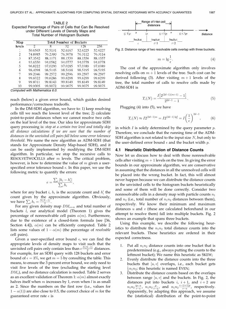
For any given density map DMoþm and total number ofbuckets l, our analytical model (Theorem 1) gives thepercentage of nonresolvable cell pairs �ðmÞ. Furthermore,due to the existence of a closed-form formula (see [36,Section 4.4]), �ðmÞ can be efficiently computed. Table 2lists some values of 1� �ðmÞ (the percentage of resolvable

cell pairs).Given a user-specified error bound �, we can find the

appropriate levels of density maps to visit such that theunvisited cell pairs only contain less than � NðN�1Þ

2 distances.For example, for an SDH query with 128 buckets and errorbound of � ¼ 3%, we get m ¼ 5 by consulting the table. Thismeans, to ensure the 3 percent error bound, we only need tovisit five levels of the tree (excluding the starting levelDMo), and no distance calculation is needed. Table 2 servesas an excellent validation of Theorem 1: �ðmÞ almost exactlyhalves itself when m increases by 1, even when l is as smallas 2. Since the numbers on the first row (i.e., values for1� �ð1Þ) are also close to 0.5, the correct choice of m for theguaranteed error rate � is

m ¼ lg1

�: ð4Þ

The cost of the approximate algorithm only involves

resolving cells on mþ 1 levels of the tree. Such cost can be

derived following (3). After visiting mþ 1 levels of the

tree, the total number of calls to resolve cells made by

ADM-SDH is

TcðNÞ ¼I�2ð2d�1Þðmþ1Þ � 1

�22d�1 � 1

: ð5Þ

Plugging (4) into (5), we have

TcðNÞ � I2ð2d�1Þm ¼ I2ð2d�1Þ lg1� ¼ I

�1

�

2d�1

; ð6Þ

in which I is solely determined by the query parameter p.

Therefore, we conclude that the running time of the ADM-

SDH algorithm is not related to the input size N , but only to

the user-defined error bound � and the bucket width p.

4.1 Heuristic Distribution of Distance Counts

Now let us discuss how to deal with those nonresolvable

cells after visitingmþ 1 levels on the tree. In giving the error

bounds in our approximate algorithm, we are conservative

in assuming that the distances in all the unresolved cells will

be placed into the wrong bucket. In fact, this will almost

never happen because we can distribute the distance counts

in the unvisited cells to the histogram buckets heuristically

and some of them will be done correctly. Consider two

nonresolvable cells in a density map with particle counts n1

and n2 (i.e., total number of n1n2 distances between them),

respectively. We know their minimum and maximum

distances u and v (these are calculated beforehand in our

attempt to resolve them) fall into multiple buckets. Fig. 2

shows an example that spans three buckets.Using this example, we describe the following heur-

istics to distribute the n1n2 total distance counts into the

relevant buckets. These heuristics are ordered in their

expected correctness.

1. Put all n1n2 distance counts into one bucket that ispredetermined (e.g., always putting the counts to theleftmost bucket); We name this heuristic as SKEW;

2. Evenly distribute the distance counts into the threebuckets that ½u; v� overlaps, i.e., each bucket gets13n1n2; this heuristic is named EVEN;

3. Distribute the distance counts based on the overlapsbetween range ½u; v� and the buckets. In Fig. 2, thedistances put into buckets i, iþ 1, and iþ 2 aren1n2

ip�uv�u , n1n2

pv�u , and n1n2

v�ðiþ1Þpv�u , respectively.

Apparently, by adapting this approach, we assumethe (statistical) distribution of the point-to-point


TABLE 2Expected Percentage of Pairs of Cells that Can Be Resolved

under Different Levels of Density Maps andTotal Number of Histogram Buckets

Computed with Mathematica 6.0.

Fig. 2. Distance range of two resolvable cells overlap with three buckets.

distances between the two cells is uniform. Thisheuristic is called PROP (short for proportional).

The assumption of uniform distance distribution in PROP

is obviously an oversimplification. In [19], we brieflymentioned a fourth heuristic: if we know the spatialdistribution of particles within individual cells, we cangenerate the statistical distribution of the distances eitheranalytically or via simulations, and put the n1n2 distances toinvolved buckets based on this distribution. This solutioninvolves very nontrivial statistical inference of the particlespatial distribution and is beyond the scope of this paper.

Note that all above methods require only constant timeto compute a solution for two cells. Therefore, the timecomplexity of ADM-SDH is not affected no matter whichheuristic is used.

5 EMPIRICAL EVALUATION OF ADM-SDH

We have implemented the ADM-SDH algorithm using theC programming language and tested it with varioussynthetic/real data sets. The experiments are run at anApple Mac Pro workstation with two dual-core 2.66-GHzIntel Xeon CPUs, and 8 GB of physical memory. Theoperating system is OS X 10.5 Leopard. In these experi-ments, we set the program to stop after visiting differentlevels of density maps and distribute the distances using thethree heuristics (Section 4.1). We then compare theapproximate histogram with those generated by regularDM-SDH. We use various synthetic and real data sets in ourexperiments. The synthetic data are generated from: 1) uni-form distributions to simulate a system with particlesevenly distributed in space; and 2) Zipf distribution withorder 1 to introduce skewness to data spatial distribution.

The real data sets are extracted from a MS of biomem-brane structures (Fig. 3). The data size in such experimentsranges from 50,000 to 12,800,000.

Table IV in Appendix I, which can be found onthe Computer Society Digital Library at http://doi.ieeecomputersociety.org/10.1109/TKDE.2012.149, sum-marizes the range and default values of the parametersused in our experiments. The code of the algorithm andthe data sets used in the experiments can be found in [39].

Fig. 5 shows the running time of ADM-SDH under onesingle p value of 2,500.0. Note that the “Exact” line showsthe results of the basic DM-SDH algorithm, whose runningtime obviously increases polynomially with N at a slope ofabout 1.5. First, we can easily conclude that the runningtime after the tree construction stage does not change withthe increase of data set size (Fig. 5a). The only exception is

when m is 5—the running time increases when N is smalland then stays as a constant afterwards. This is because thealgorithm has less than five levels to visit in a bushy treeresulted from small N values. When N is large enough,running time no longer changes with the increase of N . InFig. 5b, we plot the total running time that includes the timefor quadtree construction. Under small m values, the treeconstruction time is a dominating factor because it increaseswith data size N (i.e., OðN logNÞ). However, when m > 3,the shape of the curve does not change much as comparedto those in Fig. 5a, indicating the time for runningRESOLVETWOTREES dominates.

We observed surprising results on the accuracy ofADM-SDH. In Fig. 4, we plot the error rates observed inexperiments with three different data sets and threeheuristics mentioned in Section 4.1. First, it is obvious thatless error was observed when m increases. The exciting factis that, in almost all experiments, the error rate is lowerthan 10 percent—even for the cases of m ¼ 1! These aremuch lower than the error bounds we get from Table 2.The correctness of heuristic SKEW is significantly lowerthan that of EVEN, and that of EVEN lower than PROP, asexpected. Heuristic PROP achieves very low error rateseven in scenarios with small m values. For all experiments,the increase of data size N does not cause an increase of theerror rate of the algorithm. The above trends are observedin all three data sets. The interesting thing is, for the PROP

experiments, we can even see the trend of decreasing errorrates as N grows, especially for larger m values. We believethat serves as evidence of a (possibly) nice feature of thePROP heuristic. Our explanation is: when N is small, wecould make a very big mistake in distributing the counts inindividual operations. Imagine an extreme case in which1 distance is to be distributed into two buckets—we couldeasily get a 100 percent error in the operation. Since theerror compensation effects in PROP bring the overall errordown to a very low level (as shown in Fig. 4), PROP is moresensitive to the errors of individual distribution operationsthan SKEW and EVEN are. More in-depth explorations ofthis phenomenon are worthwhile but also beyond thescope of this paper, in which we focus on an upper boundof the error.

5.1 Discussions

At this point, we can conclude that the ADM-SDHalgorithm is an elegant solution to the SDH computationproblem. According to our experiments, extremely lowerror rates can be obtained even when we only visit as fewas one level of density map, leading to a very efficientalgorithm yet with high accuracy in practice. It is clearlyshown that the required running time for ADM-SDH growsvery slowly with the data size N (i.e., only when m is of asmall value does the tree construction time dominate).

The error rates achieved by ADM-SDH algorithmshown by current experiments are much lower than whatwe expected from our basic analysis. For example, Table 2predicts an error rate of around 48 percent for the case ofm ¼ 1, yet the error we observed for m ¼ 1 in ourexperiments is no more than 10 percent. With the PROP

heuristic, this value can be as low as 0.5 percent. Ourexplanation for such low error rates is: in an individualoperation to distribute the distance counts heuristically,we could have rendered a large error by putting too many


Fig. 3. The simulated hydrated dipalmitoylphosphatidylcholine bilayersystem. We can see two layers of hydrophilic head groups (with higheratom density) connected to hydrophobic tails (lower atom density) aresurrounded by water molecules (red dots).

counts into a bucket (e.g., bucket i in Fig. 2) than needed.But the effects of this mistake could be (partially) canceledout by another distribution operation, in which too fewcounts are put into bucket i. Note that the total error in abucket is calculated after all operations are processed;thus, it reflects the net effects of all positive and negativeerrors from individual operations. We call this phenom-enon error compensation.

While more experiments under different scenarios are

obviously needed, investigations from an analytical view-

point are necessary. From the above facts, we understand

that the bound given by Table 2 is loose. The real error

bound should be described as

� ¼ �0�00; ð7Þ

where �0 is the percentage of unresolved distances given by

Table 2, and �00 is the error rate created by the heuristics via

error compensation. In the following section, we develop an

analytical model to study how error compensation drama-

tically boosts accuracy of the algorithm.

6 PERFORMANCE ANALYSIS OF ADM-SDH

It is difficult to obtain a tight error bound for ADM-SDHdue to the fact that the error is related to data distribution.In this paper, we develop an analytical framework thatachieves qualitative analysis of the behavior of ADM-SDH,

with a focus on the generation of errors. Throughout theanalysis, we assume uniform spatial distribution of particlesand we consider only one level in the density map. At thestart level (and the only level we visit), the side length of acell is

ffiffiffi2p

p=2.

6.1 The Distribution of Two Cells’ Distance

We study two cells A and B on a density map, with cellA’s row number denoted as t and column number as j,


Fig. 4. Accuracy of ADM-SDH.

Fig. 5. Efficiency of ADM-SDH.

and cell B’s row number as k and column number as l.We further denote the minimum distance between A andB as u, and the maximum distance as v. We propose thefollowing lemma:

Lemma 1. The range ½u; v� overlaps with at most three buckets inthe SDH. In other words, p <¼ v� u <¼ 2p.

The proof of Lema 1 can be found in Appendix II,available in the online supplemental material. By Lemma 1,we can easily see that v must fall into one of the two bucketswith ranges ½bupcpþ p; bupcpþ 2pÞ and ½bupcpþ 2p; bupcpþ 3pÞ.

Suppose the distance between points from the two cellsfollow a cumulative distribution function F over the range½u; v�, then the probabilities of a distance falling into therelevant bucket can be found in Table 3.

6.2 Compensating the Distance Counts in the SKEW

Method

As mentioned earlier, an important mechanism that leads tolow error rate in our algorithm is that the errors made byone distribution operation can be compensated by those ofanother. We can use the SKEW heuristic as an example tostudy this. In SKEW, all distance counts are put into onebucket, say, the one with the smallest bucket index. In otherwords, the distance counts in all three buckets (Table 3) areput into bucket with range ½bupcp; bupcpþ pÞ. The error wouldbe large if we only consider this single distributionoperation—by denoting the error as e, we have e ¼1� F ðbupcpþ pÞ for the bucket ½bupcp; bupcpþ pÞ. The error ehere is positive, meaning counts in the first bucket areoverestimated. However, such errors can be canceled out byother distribution operations that move all distance countsfrom this bucket into another one. For example, if thereexists another distribution operation with minimum dis-tance u1 ¼ u� p, it would move some counts that belong tobucket 1 in Table 3 out, generating a negative error inbucket 1 and, thus, compensating the positive errormentioned before. Given this, an important goal of ouranalysis is to find such compensating distribution operations andstudy how much error can be compensated. We first show thatunder an ideal situation the error can reach zero.

Lemma 2. For any distribution operation with minimumdistance u, if there exists another such operation withminimum distance u1 ¼ u� p, the error generated byADM-SDH using the SKEW approach is zero.

Proof. According to Table 3, for any distribution operation,the error to the first SDH bucket (denoted as bucket i) itinvolves is 1� F ðbupcpþ pÞ, and this error is positive (i.e.,overestimation). Suppose that there is another distribu-tion with minimum distance u1 ¼ u� p, then this

operation generates a negative error F ðbupcpþ 2pÞ �F ðbupcpþ pÞ to bucket i. For the same reason, a thirddistribution with minimum distance u2 ¼ u� 2p gener-ates a negative error of 1� F ðbupcpþ 2pÞ. It is easy to seethat the combined error (by putting all relevant negativeand positive errors together) to bucket i is 0. tu

An example of two cells that contribute to each other’serror compensation in the aforementioned way can be seenin Fig. 6. Namely, the cells C and C0 when we compute theminimum distances AC and AC0.

Unfortunately, the above condition of the existence of au1 value that equals u� p cannot be satisfied for all pairs ofcells. From Lemma 2, however, we can easily see that theerror is strongly related to the quantity u. In the followingtext, we study how the errors can be partially compensatedby neighboring pairs of cells.

Without loss of generality, we take any pair of cells in thedensity map that are x cells apart horizontally and y cellsapart vertically, such as cells A and B in Fig. 6.

For the convenience of presentation, we define p to be aunit (p ¼ 1 unit). Given that fact, a cell’s side is

ffiffi2p

2 .Following this, the horizontal and vertical distancesbetween A and B are uhorizontal ¼

ffiffi2p

2 x and uvertical ¼ffiffi2p

2 y,respectively, as shown in Fig. 6. Thus, the minimumdistance between the above two cells can be written as

u ¼ffiffiffiffiffiffiffiffiffiffiffiffiffiffiffiffiffiffiffiffiffiffiffiffiffiffiffiffiffiffiffiffiffiffiffiffiffiffiffiu2horizontal þ u2

vertical

q¼

ffiffiffiffiffiffiffiffiffiffiffiffiffiffiffix2

2þ y

2

2

r: ð8Þ

The critical observation that leads to the success of ouranalysis is obtained by studying another cell, such as cell B0

in Fig. 6. Its minimum distance to the cell A is

u1 ¼

ffiffiffiffiffiffiffiffiffiffiffiffiffiffiffiffiffiffiffiffiffiffiffiffiffiffiffiffiffiffiffiffiffiffiffiffiffiffiffiðx� 1Þ2

2þ ðy� 1Þ2

2

s:

Let us denote the quantity u� u1 as �. We have

� ¼ u� u1 ¼ðu� u1Þðuþ u1Þ

uþ u1¼ u

2 � u21

uþ u1

¼x2

2 þy2

2 �ðx�1Þ2

2 � ðy�1Þ22

uþ u1� xþ y� 1

2u:

ð9Þ


TABLE 3The Buckets Involved in the Distribution of Distances from

Two Nonresolvable Cells

Fig. 6. Pairs of cells that lead to total or partial error compensation.

Suppose x >¼ y and z ¼ y=x, (9) can be rewritten as

� � xþ y� 1

2u¼

xþy�1x

2

ffiffiffiffiffiffiffiffiffix2

2 þy2

2

px

¼1þ y

x� 1xffiffiffiffiffiffiffiffiffiffiffiffiffiffiffiffiffiffiffiffiffiffiffiffi

4 x2

2x2 þ y2

2x2

� �r

¼1þ z� 1

xffiffiffiffiffiffiffiffiffiffiffiffiffiffiffi2þ 2z2p � 1þ zffiffiffiffiffiffiffiffiffiffiffiffiffiffiffi

2þ 2z2p :

ð10Þ

Although x and y are integers, we can treat z as acontinuous variable due to the existence of a large numberof possible values of x and y in a density map with manycells. Since d�=dz > 0, we conclude that � increases with z.Two boundary cases are: 1) when y ¼ 0 we have z ¼ 0 and� ¼

ffiffi2p

2 ; 2) when y ¼ x, we have z ¼ 1 and � ¼ 1.According to Lemma 2, the error of the SKEW method,

eskew, can be approximately noted by the difference betweenone and �, eskew � 1��. This error, eskewed, ranges from 0to 1�

ffiffi2p

2 , since � ranges fromffiffi2p

2 to 1. The compensatingprocess in distance counts is shown in Fig. 6. As mentionedbefore, C and C0 are examples of two cells for which thedifference of minimum distances to cell A is 1 and the cellsB and B0 are two cells for which the difference of minimumdistances is different from one (less than one in this case).

Let us analyze the minimum distances u and u1 from cellpairs ðA;BÞ and ðA;B0Þ, respectively. We know that eachsuch pair of minimum distances ðu; u1Þ with property u�u1 6¼ 1 generates an error. In the next few paragraphs, wewill quantitatively approximate the error generated by suchpair of minimum distances, and also show that the sum ofall such errors is small (can be qualitatively bounded).

Since we want to give an analytical description of aquantity ð1�� or 1� ðu� u1Þ), we need to use the under-lying distribution of that quantity. The distribution of thedistances between points from cell A and cell B (or B0) canbe viewed as noncentral chi-squared. Without loss ofgenerality, we can choose one point from cell A and makeit a base point with coordinates ð0; 0Þ. The distribution ofthe distances between this base point and points from cell B(or B0) can be regarded as triangular.

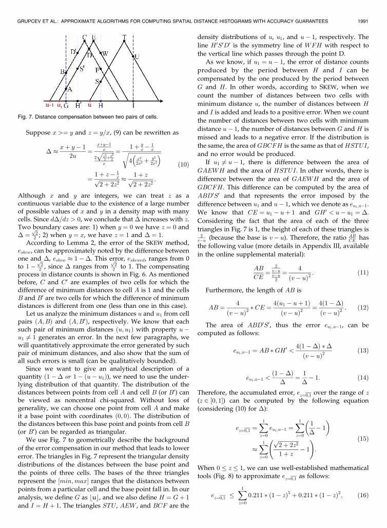
We use Fig. 7 to geometrically describe the background

of the error compensation in our method that leads to lower

error. The triangles in Fig. 7 represent the triangular density

distributions of the distances between the base point and

the points of three cells. The bases of the three triangles

represent the ½min;max� ranges that the distances between

points from a particular cell and the base point fall in. In our

analysis, we define G as buc, and we also define H ¼ Gþ 1

and I ¼ H þ 1. The triangles STU , AEW , and BCF are the

density distributions of u, u1, and u� 1, respectively. The

line H 0S0D0 is the symmetry line of WFH with respect to

the vertical line which passes through the point D.As we know, if u1 ¼ u� 1, the error of distance counts

produced by the period between H and I can be

compensated by the one produced by the period between

G and H. In other words, according to SKEW, when we

count the number of distances between two cells with

minimum distance u, the number of distances between H

and I is added and leads to a positive error. When we count

the number of distances between two cells with minimum

distance u� 1, the number of distances between G and H is

missed and leads to a negative error. If the distribution is

the same, the area of GBCFH is the same as that of HSTUI,

and no error would be produced.

If u1 6¼ u� 1, there is difference between the area of

GAEWH and the area of HSTUI. In other words, there is

difference between the area of GAEWH and the area of

GBCFH. This difference can be computed by the area of

ABD0S0 and that represents the error imposed by the

difference between u1 and u� 1, which we denote as eu1;u�1.

We know that CE ¼ u1 � uþ 1 and GH 0 < u� u1 ¼ �.

Considering the fact that the area of each of the three

triangles in Fig. 7 is 1, the height of each of these triangles is2

v�u (because the base is v� u). Therefore, the ratio ABCE has

the following value (more details in Appendix III, available

in the online supplemental material):

AB

CE¼

2v�uv�u

2

¼ 4

ðv� uÞ2: ð11Þ

Furthermore, the length of AB is

AB ¼ 4

ðv� uÞ2 CE ¼ 4ðu1 � uþ 1Þ

ðv� uÞ2¼ 4ð1��Þðv� uÞ2

: ð12Þ

The area of ABD0S0, thus the error eu1;u�1, can becomputed as follows:

eu1;u�1 ¼ AB GH 0 <4ð1��Þ �

ðv� uÞ2ð13Þ

eu1;u�1 <ð1��Þ

�¼ 1

�� 1: ð14Þ

Therefore, the accumulated error, ez¼0;1 over the range of z(z 2 ½0; 1�) can be computed by the following equation(considering (10) for �):

ez¼0;1 ¼X1

z¼0

eu1;u�1 ¼X1

z¼0

1

�� 1

�

�X1

z¼0

ffiffiffiffiffiffiffiffiffiffiffiffiffiffiffi2þ 2z2p

1þ z � 1

!:

ð15Þ

When 0 � z � 1, we can use well-established mathematicaltools (Fig. 8) to approximate ez¼0;1 as follows:

ez¼0;1 �X1

z¼0

0:211 ð1� zÞ5 þ 0:211 ð1� zÞ2; ð16Þ


Fig. 7. Distance compensation between two pairs of cells.

treating z as continuous variable we get

ez¼0;1 �Z 1

0

ð0:211 ð1� zÞ5 þ 0:211 ð1� zÞ2Þ dz

¼ 0:1055:

ð17Þ

Equation (17) means that the total error rendered by theSKEW under the assumptions we stated in the beginning ofSection 6 is less than 10.55 percent. Due to the assumptionswe made, we do not claim this as a rigorous bound.However, it clearly shows that our algorithm is able toproduce really good results with low errors by visitingonly one level in the density map. And this conclusionbuilds the foundation of an improved approximatealgorithm (Section 7).

One special note here is that (17) does not cover the casesin which the minimum distance u falls into the first SDHbucket (i.e., u < p). However, our analysis shows that suchcases do not impact the results in (17) significantly. Moredetails can be found in Appendix IV, available in the onlinesupplemental material.

7 SINGLE-LEVEL APPROXIMATE ALGORITHM

Via the performance analysis of ADM-SDH, and lookingback to the error bound described in (7), we concluded that�00 is very small. Even if we allow �0 to be 100 percent,meaning no cell resolution is possible, we can still achievelow and controllable error rates in our results. Based on suchconclusion, we introduce an improved approximate algo-rithm we call single-level SDH algorithm (SL-SDH). There aretwo major differences between the two algorithms: 1) thenumber of levels (density maps) each algorithm visits:unlike ADM-SDH, which visits mþ 1 levels, SL-SDH visitsonly one level of the tree, and is thus given the name SL-SDH.The single level visited by the SL-SDH is a user-definedvariable and can be any level of the tree. 2) the starting levelof the algorithms: ADM-SDH starts at a predeterminedlevel, based on the bucket width p and the maximumdistance between any two points of the system. SL-SDH, onthe other hand, starts at a user-defined level (and visits onlythat level), which can be any level of the tree. SL-SDHimproves over ADM-SDH in two important aspects. First,

we only need a single DM that can be built in OðNÞ time(instead of the OðN logNÞ time needed to build thequadtree). Second, we reduce the posttree-constructionrunning time of the algorithm, with little increase of theerror, as we only run RESOLVETWOTREES for cells in onedensity map (i.e., a single level).

A special note here is that the running time of SL-SDHis no longer determined by the bucket width p. Recall thatADM-SDH starts at the density map DMo, where thediagonal of a single cell is less than or equal to p. When pis small, the number of cells in DMo is large, and we haveto invoke the RESOLVETWOCELLS procedure more times.To remedy this, we allow SL-SDH to run on a (single)density map above DMo, i.e., one with larger cell sizes(and fewer cells). This is based on a hypothesis motivatedby our performance analysis of ADM-SDH: the errorcompensation mechanism we studied will also work fordensity maps above DMo. We know the error is verysmall for running RESOLVETWOTREES for those cells inDMo—doing the same on higher level density mapsshould still render reasonable (although higher) errorrates. Unfortunately, an analytical study of such errors isvery difficult. In the remainder of this section, weempirically evaluate the error and time tradeoff of thefinal version of the SL-SDH algorithm.

7.1 Experimental Results

We have implemented the SL-SDH algorithm using theC programming language and tested it with varioussynthetic/real data sets. The experiments are run in thesame environment as the experiments for the ADM-SDHin Section 5.

Since we know, from our previous experiments, that thePROP heuristic for distributing the distances in nonresol-vable cells produces the best results, we have only used thatheuristic to show the results of the single level approximatealgorithm. We have run the algorithm on two synthetic datasets (with uniform and skewed distribution of atoms) underfive different N values (i.e., 1, 3, 5, 7.5, and 12 million). Wealso ran the algorithm on one real simulation data set with891,272 atoms.

Fig. 9 shows the results from the experiments onuniform and skewed data, respectively, with 7.5 millionatoms and the real data with 891,272 atoms. From thisfigure, we can see that the error rate decreases when weincrease the level in the density map. We also see that theerror rate decreases when the bucket width increases.

Fig. 10 demonstrates the effects of system size N on theaccuracy of SL-SDH. Each line in Fig. 10 plots the errorrates of SL-SDH when run at a particular level of densitymap under a particular atom count. We can easily see thatthe lines for the five different system sizes (of the samedensity map) are very similar, giving rise to one cluster oflines for each level of density map. Fig. 10 shows that theerror introduced by the SL-SDH algorithm is not affectedby the number of atoms in the data set N , but by the levelof density map the algorithm works at. On the other hand,the running time of the SL-SDH algorithm was also foundto be independent of N , as shown in Fig. 11. The onlyexceptions are for levels 3 and 4, in which the treeconstruction time dominates.


Fig. 8. Approximation of 1�� 1 obtained in Matlab.

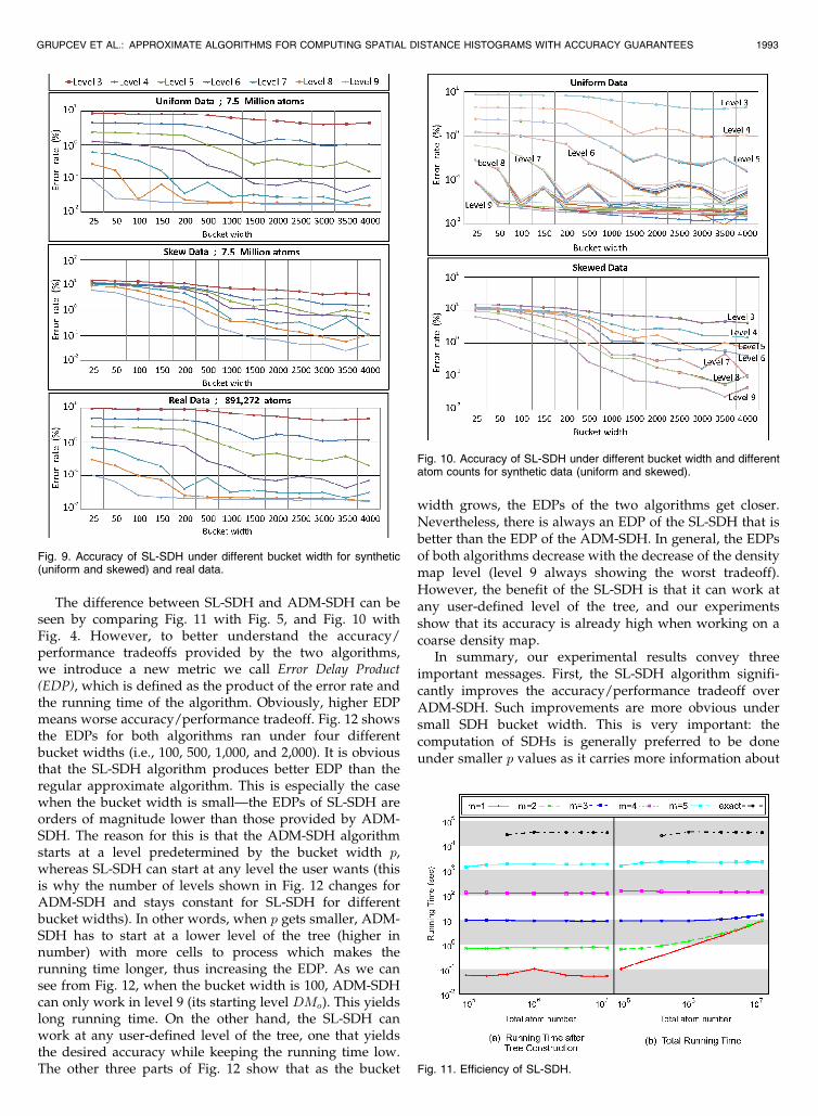
The difference between SL-SDH and ADM-SDH can beseen by comparing Fig. 11 with Fig. 5, and Fig. 10 withFig. 4. However, to better understand the accuracy/performance tradeoffs provided by the two algorithms,we introduce a new metric we call Error Delay Product(EDP), which is defined as the product of the error rate andthe running time of the algorithm. Obviously, higher EDPmeans worse accuracy/performance tradeoff. Fig. 12 showsthe EDPs for both algorithms ran under four differentbucket widths (i.e., 100, 500, 1,000, and 2,000). It is obviousthat the SL-SDH algorithm produces better EDP than theregular approximate algorithm. This is especially the casewhen the bucket width is small—the EDPs of SL-SDH areorders of magnitude lower than those provided by ADM-SDH. The reason for this is that the ADM-SDH algorithmstarts at a level predetermined by the bucket width p,whereas SL-SDH can start at any level the user wants (thisis why the number of levels shown in Fig. 12 changes forADM-SDH and stays constant for SL-SDH for differentbucket widths). In other words, when p gets smaller, ADM-SDH has to start at a lower level of the tree (higher innumber) with more cells to process which makes therunning time longer, thus increasing the EDP. As we cansee from Fig. 12, when the bucket width is 100, ADM-SDHcan only work in level 9 (its starting level DMo). This yieldslong running time. On the other hand, the SL-SDH canwork at any user-defined level of the tree, one that yieldsthe desired accuracy while keeping the running time low.The other three parts of Fig. 12 show that as the bucket

width grows, the EDPs of the two algorithms get closer.Nevertheless, there is always an EDP of the SL-SDH that isbetter than the EDP of the ADM-SDH. In general, the EDPsof both algorithms decrease with the decrease of the densitymap level (level 9 always showing the worst tradeoff).However, the benefit of the SL-SDH is that it can work atany user-defined level of the tree, and our experimentsshow that its accuracy is already high when working on acoarse density map.

In summary, our experimental results convey threeimportant messages. First, the SL-SDH algorithm signifi-cantly improves the accuracy/performance tradeoff overADM-SDH. Such improvements are more obvious undersmall SDH bucket width. This is very important: thecomputation of SDHs is generally preferred to be doneunder smaller p values as it carries more information about


Fig. 10. Accuracy of SL-SDH under different bucket width and differentatom counts for synthetic data (uniform and skewed).

Fig. 11. Efficiency of SL-SDH.

Fig. 9. Accuracy of SL-SDH under different bucket width for synthetic(uniform and skewed) and real data.

the distribution of the distances. Second, users can choosethe appropriate (single) level among all the density maps torun the algorithm based only on the desired accuracy.Third, we also show that, like ADM-SDH, the running time

and the error rate of SL-SDH are not affected by thenumber of atoms in the data set.

8 CONCLUSIONS AND FUTURE WORK

The main objective of our work is to accomplish efficientcomputation of SDH, a popular quantity in particlesimulations, with guaranteed accuracy. In this paper, weintroduce approximate algorithm for SDH query proces-sing based on our previous work developed around aQuadtree-like data structure named density map. Theexperimental results show that our approximate algorithmhas very high performance (short running time) whiledelivering results with astonishingly low error rates. Asidefrom the experimental results, we also analyticallyevaluate the performance/accuracy tradeoffs of the algo-rithm. Such analyses showed that the running time of ouralgorithm is completely independent of the input size N ,and derived a provable error bound under desiredrunning time. We further developed another mathematicalmodel to perform in-depth study of the mechanism thatleads to low error rates of the algorithm. Aside from

administering tighter bounds (under some assumptions)on the error of the basic approximate algorithm, our modelalso gives insights on how the basic algorithm can beimproved. Following these insights, a new single-levelapproximate algorithm with improved time/accuracytradeoff was proposed. Our experimental results sup-ported our analysis. Having these experimental results onhand, one aspect of our future work will be to establish aprovable error bound for the new algorithm.

Many times, the MS systems are observed over certainperiod of time and SDH computation is required for everyframe (time instance) over that period. Therefore, anotherdirection of our on-going work is to efficiently computethe SDHs of consecutive frames by taking advantage of thetemporal locality of data points. We can also extend ourwork to the computation of m-body correlation functionswith m > 2—a more general form of spatial statistics thatinvolves counting all possible m-particle tuples.

ACKNOWLEDGMENTS

The project described was supported by an Award NumberR01GM086707 from the National Institute Of GeneralMedical Sciences (NIGMS) at the National Institutes ofHealth (NIH). The authors would like to thank AnandKumar who has contributed his time and knowledgetoward realization of this paper. These authors contributedequally to this work.

REFERENCES

[1] J. Gray, D. Liu, M. Nieto-Santisteban, A. Szalay, D. DeWitt, andG. Heber, “Scientific Data Management in the Coming Decade,”ACM SIGMOD Record, vol. 34, no. 4, pp. 34-41, Dec. 2005.

[2] A.S. Szalay, J. Gray, A. Thakar, P.Z. Kunszt, T. Malik, J. Raddick,C. Stoughton, and J. vandenBerg, “The SDSS Skyserver: PublicAccess to the Sloan Digital Sky Server Data,” Proc. ACM SIGMODInt’l Conf. Management of Data, pp. 570-581, 2002.

[3] M.Y. Eltabakh, M. Ouzzani, and W.G. Aref, “BDBMS - A DatabaseManagement System for Biological Data,” Proc. Third BiennialConf. Innovative Data Systems Resarch (CIDR), pp. 196-206, 2007.

[4] M.H. Ng, S. Johnston, B. Wu, S.E. Murdock, K. Tai, H. Fangohr,S.J. Cox, J.W. Essex, M.S.P. Sansom, and P. Jeffreys, “BioSimGrid:Grid-Enabled Biomolecular Simulation Data Storage and Analy-sis,” Future Generation Computer Systems, vol. 22, no. 6, pp. 657-664,June 2006.

[5] J.M. Patel, “The Role of Declarative Querying in Bioinformatics,”OMICS: A J. Integrative Biology, vol. 7, no. 1, pp. 89-91, 2003.

[6] S. Klasky, B. Ludaescher, and M. Parashar, “The Center forPlasma Edge Simulation Workflow Requirements,” Proc. IEEEWorkshop Workflow and Data Flow for Scientific Applications(SciFlow ’06), pp. 73-73, 1991.

[7] J.L. Stark and F. Murtagh, Astronomical Image and Data Analysis.Springer, 2002.

[8] M.P. Allen and D.J. Tildesley, Computer Simulations of Liquids.Clarendon Press, 1987.

[9] D. Frenkel and B. Smit, Understanding Molecular Simulation: FromAlgorithm to Applications, series Computational Science Series,vol. 1. Academic Press, 2002.

[10] J.M. Haile, Molecular Dynamics Simulation: Elementary Methods.Wiley 1992.

[11] D.P. Landau and K. Binder, A Guide to Monte Carlo Simulation inStatistical Physics. Cambridge Univ. Press, 2000.

[12] P.K. Agarwal, L. Arge, and J. Erikson, “Indexing Moving Objects,”Proc. Int’l Conf. Principles of Database Systems (PODS), pp. 175-186,2000.

[13] M. Bamdad, S. Alavi, B. Najafi, and E. Keshavarzi, “A NewExpression for Radial Distribution Function and Infinite ShearModulus of Lennard-Jones Fluids,” Chemical Physics, vol. 325,pp. 554-562, 2006.


Fig. 12. Accuracy and performance tradeoffs of ADM-SDH and SL-SDHalgorithms under different SDH bucket widths.

[14] J.P. Hansen and I.R. McDonald, Theory of Simple Liquids. AcademicPress, 2006.

[15] A. Filipponi, “The Radial Distribution Function Probed by X-RayAbsorption Spectroscopy,” J. Physics: Condensed Matter, vol. 6,pp. 8415-8427, 1994.

[16] B. Hess, C. Kutzner, D. van der Spoel, and E. Lindahl,“GROMACS 4: Algorithms for Highly Efficient, Load-Balanced,and Scalable Molecular Simulation,” J. Chemical Theory andComputation, vol. 4, no. 3, pp. 435-447, Mar. 2008.

[17] V. Springel, S.D.M. White, A. Jenkins, C.S. Frenk, N. Yoshida, L.Gao, J. Navarro, R. Thacker, D. Croton, J. Helly, J.A. Peacock, S.Cole, P. Thomas, H. Couchman, A. Evrard, J. Colberg, and F.Pearce, “Simulations of the Formation, Evolution and Clusteringof Galaxies and Quasars,” Nature, vol. 435, pp. 629-636, June 2005.

[18] A.G. Gray and A.W. Moore, “N-Body Problems in StatisticalLearning,” Proc. Advances in Neural Information Processing Systems(NIPS), pp. 521-527, 2000.

[19] Y.-C. Tu, S. Chen, and S. Pandit, “Computing Distance Histo-grams Efficiently in Scientific Databases,” Proc. IEEE 25th Int’lConf. Data Eng. (ICDE), pp. 796-807, Mar. 2009.

[20] M. Arya, W.F. Cody, C. Faloutsos, J. Richardson, and A. Toya,“QBISM: Extending a DBMS to Support 3D Medical Images,” Proc.10th Int’l Conf. Data Eng. (ICDE), pp. 314-325, 1994.

[21] M. Stonebraker, S. Madden, D.J. Abadi, S. Harizopoulos, N.Hachem, and P. Helland, “The End of an Architectural Era (It’sTime for a Complete Rewrite),” Proc. 33rd Int’l Conf. Very LargeData Bases (VLDB), pp. 1150-1160, 2007.

[22] B. Howe, D. Maier, and L. Bright, “Smoothing the ROI Curve forScientific Data Management Applications,” Proc. Third BiennialConf. Innovative Data Systems Research (CIDR), pp. 185-195, 2007.

[23] P.G. Brown, “Overview of SciDB: Large Scale Array Storage,Processing and Analysis,” Proc. ACM SIGMOD Int’l Conf. Manage-ment of Data, pp. 963-968, 2010.

[24] M. Feig, M. Abdullah, L. Johnsson, and B.M. Pettitt, “Large ScaleDistributed Data Repository: Design of a Molecular DynamicsTrajectory Database,” Future Generation Computer Systems, vol. 16,no. 1, pp. 101-110, Jan. 1999.

[25] J. Barnes and P. Hut, “A Hierarchical O(N log N) Force-Calculation Algorithm,” Nature, vol. 324, no. 4, pp. 446-449, 1986.

[26] L. Greengard and V. Rokhlin, “A Fast Algorithm for ParticleSimulations,” J. Computational Physics, vol. 135, no. 12, pp. 280-292,1987.

[27] P.B. Callahan and S.R. Kosaraju, “A Decomposition of Multi-Dimensional Point Sets with Applications to K-Nearest-Neighborsand N-Body Potential Fields,” J. ACM, vol. 42, no. 1, pp. 67-90, 1995.

[28] L. Golab and T. Ozsu, Data Stream Management - Synthesis Lectureson Data Management. Morgan and Claypool, 2010.

[29] A.L.-O. Demaine and J.I. Munro, “Frequency Estimation ofInternet Packet Streams with Limited Space,” Proc. 10th Ann.European Symp. Algorithms, pp. 348-360, 2002.

[30] G.S. Manku and R. Motwani, “Approximate Frequency Countsover Data Streams,” Proc. 28th Int’l Conf. Very Large Data Bases,pp. 346-357, 2002.

[31] S.R. Manku and B. Lindsay, “Random Sampling Techniques forSpace Efficient Online Computation of Order Statistics of LargeData Sets,” Proc. ACM SIGMOD Int’l Conf. Management of Data,pp. 251-262, 1999.

[32] P.B. Gibbons, “Distinct Sampling for Highly-Accurate Answers toDistinct Values Queries and Event Reports,” Proc. 27th Int’l Conf.Very Large Data Bases, pp. 541-550, 2001.

[33] A. Pavan and S. Tirthapura, “Range-Efficient Computation of F0over Massive Data Streams,” Proc. 21st Int’l Conf. Data Eng., pp. 32-43, 2005.

[34] P. Flajolet and G.N. Martin, “Probabilistic Counting,” Proc. IEEEConf. Foundations of Computer Science, pp. 76-82, 1983.

[35] J. Zhou, J. Sander, Z. Cai, L. Wang, and G. Lin, “Finding theNearest Neighbors in Biological Databases Using Less DistanceComputations,” vol. 7, no. 4, pp. 669-680, 2010.

[36] S. Chen, Y.-C. Tu, and Y. Xia, “Performance Analysis of a Dual-Tree Algorithm for Computing Spatial Distance Histograms,” TheVLDB J., vol. 20, no. 4, pp. 471-494, 2011.

[37] A. Kumar, V. Grupcev, Y. Yuan, Y.-C. Tu, and G. Shen, “DistanceHistogram Computation Based on Spatiotemporal Uniformity inScientific Data,” Proc. 15th Int’l Conf. Extending Database Technol-ogy, pp. 288-299, 2012.

[38] J.A. Orenstein, “Multidimensional Tries Used for AssociativeSearching,” Information Processing Letters, vol. 14, no. 4, pp. 150-157, 1982.

[39] Y.-C. Tu, V. Grupcev, and A. Kumar, “Algorithm’s Code and DataSets,” www.cse.usf.edu/vgrupcev/tkde2012.zip, 2011.

Vladimir Grupcev received the bachelor’sdegree in applied mathematics and computerscience from the University of Ss. Cyril andMethodius, Macedonia, in 2005, the master’sdegree in mathematics from the University ofSouth Florida in 2007, and is currently workingtoward the PhD degree in the Department ofComputer Science and Engineering at theUniversity of South Florida. His area of interestincludes scientific data management and high-

performance computing. He is a student member of the IEEE.

Yongke Yuan received the PhD degree in 2003in management engineering from Peking Uni-versity in China, performed the postdoctoralstudies at Beijing University of Technology, andwas a visiting scholar at the University of SouthFlorida. He is an associate professor in theDepartment of Economics and Management atBeijing University of Technology in Beijing,China. Most of his research has focused onindustry economics such as CGE Model for

Chinese industries. His current focus is coupling natural and socialsystem science with engineering to forecast the development of Chineseindustries.

Yi-Cheng Tu received the bachelor’s degree inhorticulture from Beijing Agricultural University,China, and the MS and PhD degrees incomputer science from Purdue University in2003 and 2007, respectively. He is currently anassistant professor in the Department ofComputer Science and Engineering at theUniversity of South Florida, Tampa, Florida.His current research addresses energy-efficientdatabase systems, scientific data management,

and high-performance computing. He also worked on data streammanagement systems, self-tuning databases, peer-to-peer systems,and multimedia databases. He is a member of the IEEE, the ACM/SIGMOD, and the ASEE.

Jin Huang received the BS degree in mathe-matics from Dalian University of Technology,China, in 2004, and is currently working towardthe PhD degree in computer science at theUniversity of Texas at Arlington. His researchinterests include machine learning, data mining,and medical informatics. He is a studentmember of the IEEE.

Shaoping Chen received the bachelor’s degreein mathematics and the PhD degree in ship andmarine structures design from Wuhan Universityof Technology, China, in 1982 and 2002,respectively. He is currently an associate pro-fessor in the Department of Mathematicsat Wuhan University of Technology, Wuhan,China. He conducts research in applied mathe-matics, computer-aided geometric design, andhigh-performance computing.


Sagar Pandit received the PhD degree from theDepartment of Physics, University of Pune, in1999 in the area of dynamical systems. He is anassistant professor of physics at the Universityof South Florida. Later, his research shifted tobiological physics, specifically membrane phy-sics. His current research interests includebiomembranes, mathematical modeling of com-plex biological and social systems, dynamicalsystems, and computational approaches toward

addressing problems in these fields.

Michael Weng received the BS degree inengineering science from the Shandong Univer-sity of Science and Technology (SUST), Shan-dong, China, in 1982, the MS degree from SUSTin 1984, and the PhD degree from the Pennsyl-vania State University in 1994. He has been amember of the Department of Industrial andManagement Systems Engineering Faculty atthe University of South Florida (USF) since 1995.Prior to joining the faculty at USF, he was a senior

manufacturing engineer at Ford Motor Company. His primary areas ofresearch and scholarly work are in the fields of production planning andscheduling, supply chain management, optimization, discrete eventsimulation, and statistical modeling.

. For more information on this or any other computing topic,please visit our Digital Library at www.computer.org/publications/dlib.


1982 ieee transactions on knowledge and data...

Documents