1986 - reasoning about multiple faults · they accurately reflect the actual differences. ......

MULTIPLE FuAULTS Johan de Klcer

Intelligent Systems Laboratory XEROX Palo Alto R.esenrch Center

3333 Coyote Hill Road

Palo Alto, California 94304

and

Brian C. Williams

M.I.T. Artilicial Intelligence Laboratory

545 Technology Square Cambridge, Massachusetts, 02139

ABSTRACT

Diagnostic tasks require determining the differences

between a model of an artifact nnd the artifact itself The

differences between the manifested behavior of the artifact and th,e predicted behuvior of the model guide the setsrch

for the diflerences between the artifact and its model. The

diagnostic procedure presented in this paper is model-based, inferring the behavior of the composite device from knourl-

edge oj the structure and function of the individual compo-

nents comprising the device. The system (GDE - General

Dirtgnostic Engine) has been implemented and tested on examples in the domain of troubleshooting digital circuits.

This research makes several novel contributions: First,

the system diagnoses failures due to multiple faults. Sec-

ond, j&lure candidates are represented and manipulated in terms of minimal sets oj violated assumptions, resulting

in an eficient diagnostic procedure. Third, the diagnostic

procedure is incremental, reflecting the iterative nature of

diagnosis. Finally, a clear separation is drawn between diagnosis und behavior prediction, resulting in a domain (and injerence procedure) independent diagnostic procedure.

1. Introduction

Engineers and scientists constantly strive to under-

stand the differences between physical systems and their lllodels. Engineers troubleshoot mechanical syst,cms or

electrical circuits to find broken parts. Scientists succes- sively refine a model based on empirical data during the

process of theory formation. Many everyday common-

sense reasoning tasks involve finding the differcuce between models and reality.

Diagnostic reasoning requires a means of assigning

credit or blame to parts of the model based on observed

behavioral discrepancies observed. If the task is trou-

bleshooting, t,hen the model is presumed to be correct and

all model-artifact differences indicate part malfunctions. If the task is theory formation, then the artifact is presumed

to be correct and all model-artifact differences indicate re-

quired changes in the model. Usually the evidence does

not admit a unique model-artifact difference. Thus, the

diagnostic task requires two phases. The first, mentioned above, identifies the set of possible model-artifact diifer-

ences. The second proposes evidence-gathering tests to reline the set of possible model-artifact differences until

they accurately reflect the actual differences.

This view of diagnosis is very general, encompassing troubleshooting mechanical devices and analog and digi-

tal circuits, debugging programs, and modeling physical

or biological systems. Our approach to diagnosis is also

independent of the inference strategy employed to derive predictions from observations.

For troubleshooting circuits, the diagnostic task is to

determine why a correctly designed piece of cqltipmcnt is

not functioning as it was intended; the explanation for the faulty behavior being that the particular piece of equip-

ment under consideration is at variance in some way with

its design (e.g., a set of components is not working correctly or a set of connections is broken). To troubleshoot

a system, a sequence of measurements must be proposed,

executed and then analyzed to localize this point of variance, or fault. For example, consider the circuit in Fig. 1,

consisting of three multipliers, Ml, Mz, and Ma, and two

adders, A, and A,. The inputs are A = 3, D -x 2, C =-I 2, U = 3, and E I= 3, and the outputs are measured showing

132 / SCIENCE

From: AAAI-86 Proceedings. Copyright ©1986, AAAI (www.aaai.org). All rights reserved.

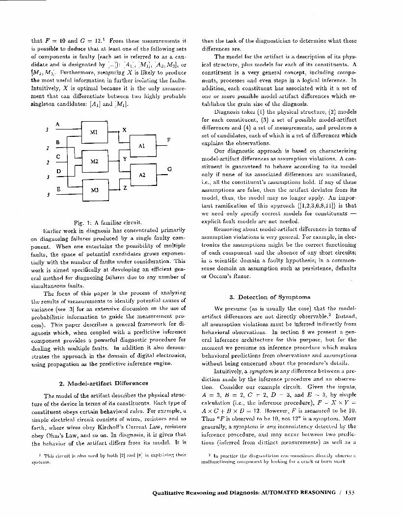
that F = 10 and G = 12.’ From these measurements it

is possible to deduce that at least one of the following sets

of components is faulty (each set is referred to as a candidate and is designated by [...I): [A,], [M,], [A2,M2], or

[AJZ, MS]. Furthermore, mea>uring X is likely to produce

the most useful information in further isolating the faults.

Intuitively, X is optimal because it is the only measure-

ment that can differentiate between two highly probable

singleton candidates: [Al] and [Ml].

A r 1 3 Ml I

B F 2 Al

I - C

2- M2 -I’

D - G 1 A2 -

Fig. 1: A familiar circuit.

Earlier work in diagnosis has concentrated primarily

on diagnosing failures produced by a single faulty com-

ponent. Wh en one entertains the possibility of multiple

faults, the space of potential candidates grows exponentially with the number of faults under consideration. This

work is aimed specifically at developing an efficient gen-

eral method for diagnosing failures due to any number of

simultaneous faults. The focus of this paper is the process of analyzing

the results of measurements to identify potential causes of

variance (see [3] f or an extensive discussion on the use of

probabilistic information to guide the measurement pro-

cess). This paper describes a general framework for di-

agnosis which, when coupled with a predictive itlference

component provides a powerful diagnostic procedure for

dealing with multiple faults. In addition it also demon- strates the approach in the domain of digital electronics,

using propagation as the predictive inference engine.

2. Model-artifact Differences

The model of the artifact describes the physical struc-

ture of the device in terms of its constituents. Each type of

constituent obeys certain behavioral rules. For csample, a

simple electrical circuit consists of wires, resistors and so forth, where wires obey Xirchoff’s Current Law, resistors

obey Ohm’s Law, <and so on. In tliaguosis, it is given that

Ihe behavior of the artifact differs frown its model. It is

I This Systclns.

cirruit is ;dso 1rwt1 by b3t.h [z] nntl [8] in cxpl:.il!ir!;; thei!

then the task of the diagnostician to determine what these

differences are.

The model for the artifact is a description of its physical structure, plus models for each of its constituents. A

constituent is a very general concept, including compo-

nents, processes and even steps in a logical inference. In

addition, each constituent has associated with it a set of

one or more possible model-artifact differences which es-

tablishes the grain size of the diagnosis. Diagnosis takes (1) the physical structure, (2) models

for each constituent, (3) a set of possible model-artifact

differences and (4) a set of measurements, and produces a

set of candidates, each of which is a set of differences which explains the observations.

Our diagnostic approach is based on characterizing

model-artifact differences as assumption violations. A constituent is guaranteed to behave according to its model

only if none of its associated differences <are manifested,

i.e., all the constituent’s assumptions hold. If any of these assumptions are false, then the artifact deviates from its

model, thus, the model may no longer apply. An impor-

tant ramification of this approach ([1,2:3,6,8,11]) is that WC need only specify correct models for constituents -

explicit fault models <are not needed.

Reasoning about model-artifact differences in terms of

assumption viol&ons is very general. For example, in electronics the assumptions might be the correct functioning

of each component and the absence of any short circuits;

in a scientific domain a faulty hypothesis; in a common-

sense domain an assumption such as persistence, defaults or Occam’s Razor.

3. Detection of Symptoms

We presume (as is usually the case) that the model-

artifact differences are not directly observable.2 Instead,

all assumption violations must be inferred indirectly from

behavioral observations. In section 8 we present a general inference architecture for this purpose, but for the

moment we presume an inference procedure which makes

behavioral predictions from observations and assumptions without being concerued about the procedure’s details.

Intuitively, a symptom is any difference between a pre-

diction made by the inference procedure and an observa-

tion. Consider our example circuit. Given the inputs,

A = 3, B = 2, C = 2, D = 3, and E = 3, by simple

calculation (i.e., the inference procedure), F = X x 1’ =

A x C + R x D = 12. However, F is measured to be 10.

Thus “J’ is observed to be 10, not 12” is a symptom. More

generally, a symptom 1. .C u,ny inconsistency detected by the

inference proccdurc, and way occur ber.wecn two prcdic-

tions (inl’erred from distinct oleasureiuents) as well as n

Qualitative Reasoning and Diagnosis: AUTOMATED REASONING / 133

measurement and a prediction (inferred from some other

measurements).

4. Conflicts

The diagnostic procedure is guided by the symptoms.

Each symptom tells us about one or more assumptions

that are possibly violated (e.g., components that nmy be

faulty). Intuitively, a conflict is a set of assumptions sup-

porting a symptom, and thus leads to an inconsistency. In electronics, a conflict might be a set of components which

cannot all be functioning correctly. Consider our example sylllptonl “F is observed to be 10, not 12.” Our calcu-

lation that E’ = 12 depends on the correct operation of Ml, M2 and Al, i.e., if Ml, A42, and A, were correctly functioning, then F = 12. Since F is not 12, at least one

of Ml, M2 and Al is faulted. Thus the set (Mi,M2,Ai) (conIlicts are indicated by (...)) is a conflict for the synlp-

tom. Because the inference is monotonic with the set of

assumptions, the set (Ml, M’2, Ai, AZ), and any other su-

perset of (Ml, Mz, Al) are conflicts as well; however, no subsets of (Ml, M;!, Al) are necessarily confticts since all the components in the conflict were necessary to constrain

the value at F.

A measurement might agree with one prediction and yet disagree with another, resulting in a symptom. For example, starting with the inputs B = 2, C = 2, D = 3, and E = 3, <and assuming M2, MS and A2 are correctly

funct,ioning we calculate G to be 12. However, starting with the observation F = 10, the inputs A = 3, C = 2, and E = 3, and assuming that Al, AZ, Ml, and MS, (i.e.,

ignoring 1W2) arc correctly functioning we calculate G =

10. Thus, when G is measured to be 12, even though it

agrees with the first prediction, it still produces a conflict

based on the second: (Al, AZ, Ml, MS).

For complex domains any single symptom can give rise to a large set of comlicts, including the set of all com-

ponents in the circuit. To reduce the combinatorics of

diagnosis it is essential that the set of conflicts be represented and manipulated concisely. If a set of components

is a conflict, then every superset of that set must also be a

conflict. Thus the set of conflicts can be represented concisely by only identifying the minimal conIlicts, where a

conflict is minimal if it has no proper subset which is also

a conflict. This observation is central to the performance

of our diagnostic procedure. The goal of conflict recognition is to identify the complete set of minimal conIlicts.3

‘JJyJ>ically, but not always, each symptom corresponds to a

single minimal conflict.

5. Candidates

A cnndidate is a particular hypothesis for how the ac-

tual artifact differs from the model. Ultimately, the goal of diagnosis is to identify, and refine, the set of candidates

consistent with the observations thus far.

A candidate is represented by a set of assumptions

(indicated by [...I). Every assumption mentioned in the

set must fail to hold. As every candidate must explain

every symptom (i.e., its conflicts), each set representing a

candidate must have a non-empty intersection with every

conflict.

For electronics, a candidate is a set of failed components, where (any components not mentioned a.re guaran-

teed to be working. Before any measurements have been

taken we know nothing about the circuit. The size of the

initial candidate space grows exponentially with the num-

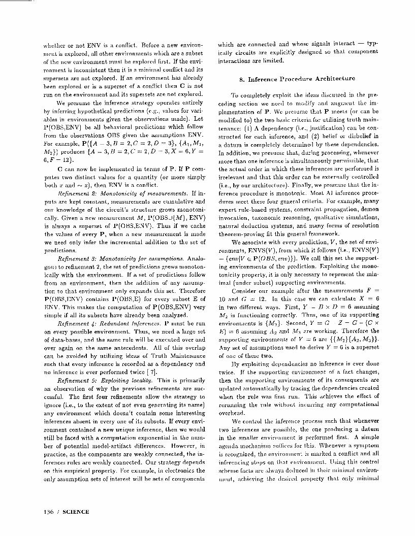
ber of components. Any component could be working or faulty, thus the candidate space for Fig. 1 initially consists of 2” = 32 candidates.

[MI.M2.Ml.Al.A2)

[MI.MZ.MJ.Al)

[Mull PfMwI &i%All IMU9 [AL421

Fig. 2 Initial candidate space for circuit example.

It is essential that candidates be represented concisely

as well. Notice that, like conflicts, candidates have the

property that any superset of a candidate must be a can-

didate as well. Thus the space of all candidates consistent

with the observations can be represented by the minimal

candidates. The goal of candidate generation is to idcn- tify the complctc set of niinimnl candidates. The space of

candidates can be vislinlixed in tcrri1s of a slll)sct,-snI)cl.,~ct

l;~tlicf: (Fig. 2). ‘1‘1 ic tnirliurnl camflitl~~lcs tltcn flcfitie a

bonritli~ry suc!i t.hat f~vcrytliing fro~il Idie boundary up is a vnlifl candidate, ;vhilc: everything below is not.

Given no measurements every component might be

working correctly, thus the single minimal candidate is the

empty set, [], which is the root of the lattice at the bottom

of Fig. 2.

To summarize, the set of candidates is constructed in

two stages: conflict recognition and candidate generation.

ConIlict rccoguition uses the observations made along with

a model of t,he device to construct a complete set of min-

134 / SCIENCE

imal conflicts. Next, candidate generation uses the set of

minimal conflicts to construct a complete set of minimal candidates. Candidate generation is the topic of the next

section, While conflict recognition is discussed in Section

7.

0. Candidate Generation

Diagnosis is an incremental process; as the amgnos-

tician takes measurements he continually relines the can-

didate space and then uses this to guide further measurements. Within a single diagnostic session the total set of

candidates must decrease monotonically. This corresponds

to having the minimal candidates move monotonically up

through the candidate superset lattice towards the candi-

date represented by the set of all components. Similarly,

the total set of conflicts must increase monotonically. This corresponds to having the minimal conflicts move mono-

tonically down through a conflict superset lattice towards

the conflict represented by the empty set. Candidates care generated incrementally, using the new conflict(s) and the

old candidate(s) to generate the new candidate(s).

The set of candidates is incrementally modified as follows. Whenever a new conflict is discovered, any previous

minimal candidate which does not explain the new con-

flict is replaced by one or more superset candidates which are minimal based on this new information. This is ac-

complished by moving up along the lattice from the old

minimal candidate, recording the first candidate reached which explains the new conflict; i.e., when the candidate’s

intersection with the new conflict is non-empty. When

moving up past a candidate with more than one parent a consistent candidate must be found along each branch.

Eliminated from those candidates recorded are any which

are subsumed or duplicated; the remaining candidates are

added to the set of new candidates.

Consider our example. Initially there are no conflicts, thus the minimal candidate [] (i.e., everything working)

explains all observations. We have already seen that the

single symptom “F = 10 not 12” produces one conflict

(A,, Ml, Mz). This rules out the single minimal candidate [I. Thus, its immediate supersets [Ml], [Mz], [MS], [Al],

and [AZ] are examined. Each of the candidates [MI], [Mz],

and [A,] explain the new conflict and thus are recorded;

however, [AZ] and [MS] do not. All of their immediate

superset candidates except for [AZ, MS] are supersets of the three minimal candidates discovered above. [AZ, MS]

does not explain the new conflict, however, its immedi-

ate superset candidates are supersets of the three minimal

candidates and thus are implicitly represented. Therefore,

the new minimal candidate set consists of [Ml], [Mz], and

[AI]. The second conflict (infcrrcd from observation G ==

1% (4, A2, Ml, MA only eliminates minimal Catldidid!

[&fz]; the unaffected candidntcs [Ml], aud [ tll] remain min-

imal. Ijowever, to complete the set of minimal candidates

we must consider the supersets of [Mz]: [Al, Mz], [A2, n/r,],

[W, M2], an d [M2, M3]. Each of these candidates explains

the new conflict, howcvcr, [A,,MzJ and [n/r,, M21 are SU-

persets of the minimal candidates [Al] ad [MI], respec- tjvely. Thus the new minimal candidates are [A2, n/iz], and

[p/f2, M3], resulting in the Il;inimal candidate set: [Al],

[Ml], [AZ, Mz], and [Mz, Mz]. Candjdate generation has several interesting proper-

ties: First, the set of minimal candidates may increase or decrease in size as a result of a measurement; however, a

candidate, once eliminated can never reappear. AS measurements accumulate the sizes of the minimal candidates

never decrease. Second, if an assumption appears in every

minimal candidate (and thus every candidate), then that

assumption is necessarily false. Third, the presupposition

that there is only a single fault (exploited in all previous

model-based troubleshooting strategies), is equivalent to

assuming all candidates are singletons. In this case, the set of candidates can be obtained by intersecting all the

conflicts.

7. Conflict Recognition Strategy

The remaining task involves incrementally constructing the conflicts used by candidate generation. In this sec-

tion we first present a simple model of conflict recognition.

This approach is then refined into an efficient strategy. A conflict can be identified by selecting a set of as-

sumptions, referred to as an environment, and testing if they are inconsistent with the observations.4 If they are, then the inconsistent environment is a conflict. This re-

quires an inference strategy C(OBS,ENV) which given the

set of observations OBS made thus far, and the cnviron-

merit ENV, determines whether the combination is consis-

tent. In our example, after measuring F = 10, and before

measuring G = 12, C({F = lo}, {M~,M2,A,}) (leaving off the inputs) is false indicating the conflict (Ml, M2, Al).

This approach is refined as follows:

Refinement I: Exploiting minimality. To identify the

set of minimal inconsistent environments (and thus the

minimal conflicts), we begin our search at the empty environment, moving up along its parents. This is sinlilar

to the search pattern used during candidate generation.

At each environment we apply C(OBS,ENV) to dcterrnine

4 An environment should not be confused with n calldidnte. An environment is n set of assumptions all of which are assnrned to be true (e.g., A41 alld M2 WC CSSII I~~CI to bc working correctly), a cnndidntc is a set of assumptions all of which arc assumed to be false (e.g., colllpollents Ml and A42 are liot fuuctionillg correctly). A conflict is n, set of ;lssun~~~l.iolls, at least one of which is f&c. Intuitivrly an rnvironmtmt is t,bc% set of assulllptions tlmt defijl:? il "contc!ut" in a deductive infc~rcrtcc engin(B, in this cnx: t,llc engilM2 i:; IISCX~ for pdict.iotr and t.ho assurnpt,iom ;IIC ;hout the 1:lck of particular n~otlcl-artifact dilfcrctlccs.

Qualitative Reasoning and Diagnosis: AUTOMATED REASONING / 13 j

whether or not ENV is a conflict. Before a new environ-

ment is explored, all other environments which are a subset

of the new environment must be explored first. If the environment is inconsistent then it is a minimal conflict and its

supersets are not explored. If an environment has already been explored or is a superset of a conflict then C is not

run on the environment and its supersets are not explored.

We presume the inference strategy operates entirely

by inferring hypothetical predictions (e.g., values for vnri-

ables in environments given the observations made). Let

P(OBS,ENV) b e all behavioral predictions which follow

from the observations OBS given the assumptions ENV.

For example, P({A = 3,B = 2,C = 2,D = 3}, {Al,Ml, Mz}) produces {A = 3, B = 2, C == 2,D = 3,X = 6, Y =

6, F = 12).

C can now be implemented in terms of P. If P com-

putes two distinct values for a quantity (or more simply both z and - TC), then ENV is a conflict.

Refinement 2: Monotonicity of measurements. If in-

puts are kept constant, measurements are cumulative and our knowledge of the circuit’s structure grows monotoni-

cally. Given a new measurement M, P(OBSU{M}, ENV)

is always a superset of P(OBS,ENV). Thus if we cache

the values of every P, when a new measurement is made

we need only infer the incremental addition to the set of predictions.

Refinement 3: Monotonicity for assumptions. Analo-

gous to refinement 2, the set of predictions grows monoton-

ically with the environment. If a set of predictions follow

from an environment, then the addition of any assumption to that environment only expands this set. Therefore

P(OBS,ENV) contains P(OBS,E) for every subset E of

ENV. This makes the computation of P(OBS,ENV) very simple if all its subsets have already been analyzed.

Refinement 4: Redundant Inferences. P must be run

on every possible environment. Thus, we need a large set

of data-bases, and the same rule will be executed over and

over again on the same antecedents. All of this overlap can be avoided by utilizing ideas of Truth Maintenance

such that every inference is recorded as a dependency and no inference is ever performed twice [ 71.

Refinement 5: Exploiting locality. This is primarily

an observation of why the previous refinements care suc-

cessful. The first four refinements allow the strategy to ignore (i.e., to the extent of not even generating its name)

any enviromnent which doesn’t contain some interesting

inferences absent in every one of its subsets. If every envi-

ronment contained a new unique inference, then we would

still be faced with a computation exponential in the num-

bcr of potential model-artifact differences, However, in

practice, as the components are weakly connected, the in-

ferences rules are weakly connected. Our strategy depends

on this empirical property. For example, in electronics the

only assumption sets of interest will be sets of components

which are connected and whose signals interact - typ-

ically circuits are explicitly designed SO that colllporlent

interactions are limited.

8. Inference Procedure Architecture

To completely exploit the ideas discussed in the pre-

ceding section we need to moclify and augmcn t, Ihe itn-

plementation of P. We presume that P meels (or can be

modified to) the two basic criteria for utilizing truth main-

tenance: (1) A dependency (i.e., justification) can be con-

structed for each inference, and (2) belief or disbelief in

a datum is completely determined by these dependencies.

In addition, we presume that, during processing, whenever more than one inference is simultaneously permissible, that

the actual order in which these inferences are performed is

irrelevant and that this order can be ext.ernally controlled (i.e., by our architecture). Finally, we presume that the in-

ference procedure is monotonic. Most Al inference proce-

dures meet these four general criteria. For example, many

expert rule-based systems, constraint propagation, demon invocation, taxonomic reasoning, qualitative simulations,

natural deduction systems, and many forms of resolution

theorem-proving fit this general framework.

We associate with every prediction, V, the set of envi-

ronments, ENVS(V), from which it follows (i.e., ENVS(V) E {envlV E P(OBS, env)}). We call this set the support-

ing environments of the prediction. Exploiting the mono-

tonicity property, it is only necessary to represent the minimal (under subset) supportiug environments.

Consider our example after the measurements F =

10 and G = 12. In this case we can calculate X = 6

in two different ways. First, Y = B x 15) = 6 assuming

n/r, is functioning correctly. Thus, one of its supporting environnlents is {Mz}. Second, Y = G - 2 = G - (C x

I;-‘) == 6 assl~ming 112 and ,‘l13 nre working. Therefore the

supporting environments of Y := 6 are {{Mz}{A:!, MS}). Any set of assumptions used to derive Y = G is a superset

of one of these two.

By exploitin, m dependencies no inference is ever done

twice. If the supporting environment of a fact changes,

then the supporting environments of its consequents are

updated automatically by tracing the dcpcndencies created

when the rule was first, run. l’his achieves the effect of

rerunning the rule without incurring any computational

overhead,

Wc control the inference IJrixCSS such that whenever

two inFerenccs are posslhle, the one producing a datum

in the smaller environment is performed first. A simple

agenda lJlCChc?~JiSlll srlIfices for this. Whenever a symptom

is rccoguizcd, the enviroamcnl is marked a conflict and all

inf::ro~icing stops on lhat or:‘* -iron nlcut. Using this control

schr~lle facts are ;dwnys dctlucetl in their nlinilual environ-

IllClJi,, ;Lcllicving oho dcsircd property th,at only minimal

136 I SCIENCE

conflicts (i.e., inconsistent environments) arc geueratcd.

In this architecture P can be incomplete (in praclice it

usually is). The only consequence of incolnplcteness is that

fewer conflicts will be detected and thus fewer candidates will be eliminated than the ideal - no candidate will be

mistakenly eliminated.

9. Circuit Diagnosis

Thus far we have descrihcd a very general diagnos-

tic strategy for handling multiple faults: whose application to a specific domain depends only on the selection of

the function P. During the remainder of this paper, WC

demonstrate the power of this approach, by applying it to

the problem of circuit diagnosis. For our example we make a number of simplifying pre-

suppositions. First, we assume that the model of a circuit

is described in terms of a circuit topology plus a behavioral description of each of its components. Second, that the

only type of model-artifact difference considered is whether

or not a particular component is working correctly. Fi- nally, all observations are made in terlns of measurements

at a component’s terminals. Measurements are expensive,

thus not every value at every terminal is known. Instead,

some values must be inferred from other values and the

component models. Intuitively, symptoms are recognized by propagating out locally through components from the

measurement points, using the component models to deduce new values. The application of each model is based

on the assumption that its corresponding component is

working correctly. If two values are deduced for the same

quantity in different ways, then a coincidence has occurred.

If the two values differ then the coincidence is a symptom. The conflict then consists of every component propagated

throng11 from the measurement points to the point of coin-

cidence (i.e., the sympt,om implies that, at least one of the

components used to deduce the two values is inconsistent,).

10. Constraint Propagation

Constraint propagation [12,13] operates on cells, val-

ues, and constraints. Cells represent state variables such

as voltages, logic levels, or fluid flows. A constraint stipu-

lates a condition that the cells must satisfy. For example, Ohm’s law, ZI = iR, is represented as a constraint among

the three cells V, i, and R. Given a set of initial values,

constraint propagation assigns each cell a value that sat-

isfies the constraints. The basic inference step is to find

a constraint that allows it to determine a value for a pre-

viously unknown cell. For example, if it has discovered

values v = 2 and i = 1, then it rises the constraint v = iR

to calculate the value R = 2. In addition, the propa.gnt,or

records If’s depclltloricy on 21, i and the constraitit 1~ -z ill.

The newly recorded value ~lrny cnusc other conslrnints to

trigger and more values to be deduced. Thus, constraints

may be viewed as a set of conduits along which values can

be propagated out locally from the inputs to other cells in

the system. The dependencies recorded trace out a particular path through the constraints that the inputs have

taken. ,i synlptom is manifcstcd when two different values

are deduced for the same cell (i.e., a logical inconsistency

is identified). In this event dependencies are used to con-

struct the conflict.

Sometimes the constraint propagation process tcrmi-

nates leaving some constraints unused and some cells unas-

signed. This usually arises as a consequence of insufficient informatiou about device inputs. However, it can also =arise

as the consequence of logical incompleteness in the propagator.

In the circuit domain, the behavior of each component

is modeled as a set of constraints. For example, in analya-

ing analog circuits the cells represent circuit voltages and currents, the values are numbers, and the constraints are

mathematical equations. In digital circuits, the cells repre-

sent logic levels, the values are 0 and t, and the constraints are boolean equations.

Consider the constraint model for the circuit of Fig.

1. There are ten cells: A, B, C, D, E, X, Y, 2, F, and

G, five of which are provided the observed values: A = 3, B = 2, C = 2, D = 3 and E = 3. There are three lnultipliers and two adders each of which is modeled by

a single constraint: MI : X = A x C, M, : Y = I3 x D, MS : 2 = CXE, AI : F = X+Y, and A2 : G = Y+Z. The

following is a list of cleductions and dependencies that the constraint propagator generates (a dependency is indicated

by (component : antecedents):

X=6(MI:A=3,C=2)

Y=6(M2:B=2,D=3)

Z=6 (M3:C=2,E=3)

F=12(Al:X=6,Y=6)

G=12(AZ:Y=6,Z=6)

A symptom is indicated when two values are detcrnlincd

for the same cell (e.g., measuring F to be 10 not 12). Each symptom leads to new conflict(s) (e.g., in this example the

symptom indicates a conflict (A,, MI, Mz)), This approach has some important properties. First,

it is not necessary for the starting points of these paths

to be inputs or outputs of the circuit. A path may begin

at, any point in the circuit where a measurement has been

taken. Scconcl, it is not necessary lo make any assumy- tions about Ilie direction that sigllnls flow tliroiigh conipo-

ncnts. Tn most digital circuits a signal can only flow from

inputs to outputs. For cxa~l~plc, a subtracI.or cannot bc

constructed by sinlply reversing xi input ,and the output


of an adder since it violates the directionality of signal flow.

However, the directionality of a component’s signal flow is irrelevant to our diagnostic technique: a component places a constraint between the values of its terminals which can

be used any way desired. To detect discrepancies, infor-

mation can flow along a path through a component in any

direction. For example, although the subtractor does not function in reverse, when we observe its outputs we can

infer what its inputs must have been.

11. Generalized Constraint Propagation

Each step of constraint propagation takes a set of an-

tecedent values and computes a consequent. We have built

a constraint propagator within our inference architecture

which explores minimal environments first. This guides

each step during propagation in an efficient manner to incrementally construct minimal conflicts and candidates for

multiple faults. Consider our example. We ensure that propagations

in subset environments are performed first, thereby guar-

anteeing that the resulting supporting environments and conflicts arc minimal. We use 15, el, e2, . ..I to represent the

assertion x with its associated supporting environments.

Before any measurements or propagations take place, given

only the inputs, the data base consists of: [A = 3, {}I, [B = 2, {}], [[C = 2, {>], [[D = 3, -OD, and UE = 3, On- Observe that when propagating values through a component, the assumption for the component is added to the

dependency, and thus to the supporting environment(s)

of the propagated value. Propagating A and C through

Ml we obtain: [[X = 6, {Ml}]. The remaining propa-

gations produce: [[Y = 6, w2)n, uz = 6, w3n up =

12, {AI, wafdn, and [G = 12, (A2, M2, it&}]. Suppose we measure F to be 10. This adds [IF =

10, {}I to t,he data base. Analysis proceeds as follows

(starting with the smaller assumption sets first): [[X =

4, {Al,M2}~, and [Y = 4, {Al,Ml}j. NOW the symptom between [[F = 10, {}I and [TF = 12, {Al, Ml,M2}~ is rec-

ognized indicating a new minimal conflict: (Al, MI, M2). Thns the inference architecture prevents further propaga-

tion in the environment {Al, Ml, Mz} and its supersets.

The propagation goes one more step: [G = 10, {Al, AZ, MI, MS}]. There are no more inferences to be made.

Next, suppose we measure G to be 12. Propaga-

tion gives: [I2 = 6, {A2,M3}], [Y = 6, {&,~I~}], 12 = 8, (4, A2, MIIII, and [X = 4, {A 1, A2, &}]. The symp-

tom “G = 12 not 10” produces the conflict (Al,A,, Ml, MS). The final data-base state is:5

A= 3,0 B= 2,{) c= 2,o

D= 3,0 E= 390 F= lO,{}

G= 12,{}

X = 4, (AI, j&&G, Ad&)

ww

Y I= 4, {Al, M,} %{M2}{Az,M3)

Z = 8, {&,~MI)

6,{M3}{A2,M2) This results in two minimal conflicts:

(AI, 4, Mdf3) Note that at no point during propagation is effort

wasted in constructing non-minimal conflicts.

The algorithm discussed in section 6 uses the two minimal conflicts to incrementally construct the set of mini-

mal candidates. Given new measurements the propaga-

tion/candidate generation cycle continues until the candidate space has been sufficiently constrained

12. Connected Research

Our approach has been completely implemented and

tested on numerous examples. Our implementation consists of four basic modules. The first maintains the mini-

mal supporting environments for each prediction and constructs minimal conflicts. It is based on Assumption-Based

Truth Maintenance [4]. Tl le second controls the inference such that minimal conflicts are discovered first and records the dependencies of inferences. It is based on the consumer

and agenda architectures of [5]. The third is a general con-

straint language based on the first two modules. The last module, the candidate generator, incrementally constructs

the minimal candidates from the minimal conflicts.

As all the work within the model-based paradigm, our

approach presumes measurements and potential model-

artifact differences are given. In [3] we exploit the framework of this paper in two ways to generate measurements

which are information-theoretically optimal. First, the data structures constructed by our strategy (e.g., the data

base state of Section 11) make it easy to consider and eval-

uate hypothetical measurements. Second, as we construct

all minimal environments, conflicts, and candidates, it is

relatively straight forward to compare potential measurements (using probabilistic information of component fail-

ure rates).

The work presented here represents <another step to-

wards Ihe goal of automatecl diagnosis, nevcrthcless there

remains much to be done. Plans for the future include:

1) incorpornling the predictive cnginc cliscussed in [14] in

order to diagnosis systcn~s with time-varying signals and

138 / SCIENCE

state, and 2) controlling the set of model-artifact differ-

ences being considered.

13. Related Work

This research fits within the model-based debugging

paradigm: [1,2,3,6,8, 9,111. However, unlike [1,2,6,8, 91, we propose a general method of diagnostic reasoning which is

effic.ient, incremental, handles multiple faults, and is easily

extended to include measurement strategies. Reiter (111

has been exploring these ideas independently and provides

a formal account of many of our “intuitive” techniques of

conIlict recognition and candidate generation.

ACKNOWLEDGMENTS

Daniel G. Bobrow, Randy Davis, Kenneth Forbus, Matthew Ginsberg, Frank Halasz, Walter Hamscher, Tad

Hogg, Ramesh Patil, provided useful insights. We espe-

cially thank Ray Reiter for his clear perspective <and many

productive interactions.

BIBLIOGRAPHY

1. Brown, J.S., Burton, R. R. and de Kleer, J., Peda- gogical, natural language and knowledge engineering

techniques in SOPHIE I, II and III, in: D. Sleeman

and J.S. Brown (Eds.), Intelligent Tutoring Systems, (Academic Press, New York, 1982) 227-282.

2. Davis, R., Shrobe, H., Hamscher, W., Wieckert, K.,

Shirley, M. and Polit, S., Diagnosis based on description of structure and function, in: Proceedings of the

National Conference on Artificial Intelligence, Pitts-

burgh, PA (August, 1982) 137-142.

3. de Kleer, J. and Williams, B.C., Diagnosing multiple

faults, Artificial Intelligence (1986) forthcoming. 4. de Kleer, J., An assumption-based truth maintenance

system, Artificial Intelligence 28 (1986) 127--162. 5. de Kleer, J., Problem solving with the ATMS, Artifi-

cial Intelligence 28 (1986) 197-224.

6. de Kleer, J., Local methods of localizing faults in

electronic circuits, Artificial Intelligence Laboratory, AIM-394, Cambridge: M.I.T., 1976.

7. Doyle, J., A truth maintenance system, Artificial In-

telligence 24 (1979). 8. Genesereth, M.R., The use of design descriptions in

automated diagnosis, Artificial Intelligence 24 (1984),

411-436.

9. Hamscher, W., and Davis, R.., Diagnosing circuits with

state: an inhcrcntly undcrconstraincd problem, in:

Proceedings of the National Conference on Artificia.1

Intelligence, Austin, TX (August, 1984) 142 -147.

10.

11.

12.

13.

14.

Mitchell, T., Version spaces: An approach to concept

learning, Computer Science Department, STAN-CS- 78-711, Palo Alto: Standford University, 1978.

Reiter, R., A theory of diagnosis from first principles,

Artificial Intelligence, forthcomming. Also: Depart-

ment of Computer Science Technical Report 187/86,

(University of Toronto, Toronto, 1985).

Steele, G.L., The dcEnition and implementation of a computer programming language based on constraints,

AI Technical Report 595, MIT, Cambridge, MA, 1979.

Sussman, G.J. and Steele, G.L., CONSTRAINTS: A language for expressing almost-hierarchical descriptions, Artificial Intelligence 14 (1980) l-39.

Williams, B.C., “Doing Time: Putting Qualitative

Reasoning on Firmer Ground,” Proceedings of the Nu- tional Conference on Artificial Intelligence, Philadel-

phia, Penn., (August, 1984).


1986 - reasoning about multiple faults · they accurately reflect the actual differences. ......

Documents