1q2015-part1-bloesch-gourio-pdf (1)

1Federal Reserve Bank of Chicago

The effect of winter weather on U.S. economic activity

Justin Bloesch and François Gourio

Introduction and summary

The unusually cold and snowy 2013–14 winter substan-tially disrupted the routines of people across the United States, leading commentators and policymakers to ask if the weather affected economic activity as well. There were many media stories that supported this hypothesis. For instance, some employees were reported as unable to com-mute to work, and some projects, particularly in con-struction, were delayed due to equipment limitations or concerns about safety in the cold and snow. Supply chains were sometimes interrupted; for instance, steel production along the coast of Lake Michigan was affected because the boats delivering iron ore were unable to navigate the deeply frozen Great Lakes. Furthermore, retailers reported that households may have delayed shopping due to ex-treme weather. And finally, some expected that the higher heating costs and the expenses for home repairs (such as burst pipes) would hamper consumer spending.

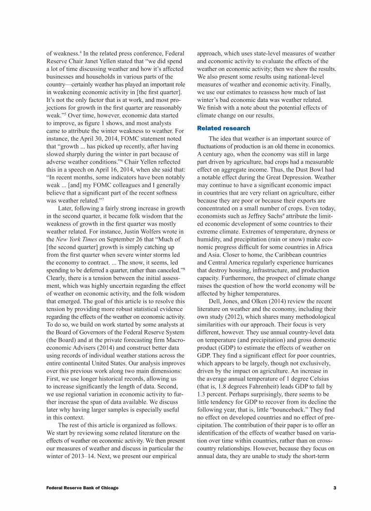
Consistent with these anecdotes, economic indica-tors published early in 2014, such as industrial produc-tion, employment, and car sales, showed that economic activity had slowed substantially in December 2013 and January 2014. While the economic recovery following the Great Recession had appeared to accelerate in the fall of 2013, these statistics suggested a renewed slow-down. To illustrate these patterns, figure 1 depicts the evolution of several economic indicators:1 the monthly change in nonfarm employment, the National Associ-ation of Purchasing Managers (NAPM) Index, light-weight vehicle sales, retail sales (excluding auto sales), manufacturing industrial production, and the Chicago Fed National Activity index (CFNAI), which itself summarizes a variety of indicators. These indicators are seasonally adjusted using statistical methods, which amounts to removing the effects of a “normal winter.” In these figures, the three red dotted points correspond to December 2013, January 2014, and February 2014, respectively. The decline of these indicators during the December to February period is consistent with a

slowdown in economic activity due to the weather, but could also have reflected other sources of weakness. Indeed, there was much controversy at the time on how much of the decline in the indicators was driven by the bad weather as opposed to other factors. The conventional wisdom was that a slowdown in economic activity due to weather would be very temporary; projects that had been delayed due to weather would eventually be finished and consumer shopping would likely resume.

Justin Bloesch is an associate economist and François Gourio is a senior economist in the Economic Research Department at the Federal Reserve Bank of Chicago. The authors thank their colleagues at the Chicago Fed and Lisa Barrow, Olivier Deschênes, Charles Gilbert, Ben Herzon, Alejandro Justiniano, and Thomas Klier for useful discussions and feedback.© 2015 Federal Reserve Bank of Chicago Economic Perspectives is published by the Economic Research Department of the Federal Reserve Bank of Chicago. The views expressed are the authors’ and do not necessarily reflect the views of the Federal Reserve Bank of Chicago or the Federal Reserve System.Charles L. Evans, President; Daniel G. Sullivan, Executive Vice President and Director of Research; Spencer Krane, Senior Vice President and Economic Advisor; David Marshall, Senior Vice President, financial markets group; Daniel Aaronson, Vice President, microeconomic policy research; Jonas D. M. Fisher, Vice President, macroeconomic policy research; Richard Heckinger, Vice President, markets team; Anna L. Paulson, Vice President, finance team; William A. Testa, Vice President, regional programs; Lisa Barrow, Senior Economist and Economics Editor; Helen Koshy and Han Y. Choi, Editors; Rita Molloy and Julia Baker, Production Editors; Sheila A. Mangler, Editorial Assistant.Economic Perspectives articles may be reproduced in whole or in part, provided the articles are not reproduced or distributed for commercial gain and provided the source is appropriately credited. Prior written permission must be obtained for any other reproduc-tion, distribution, republication, or creation of derivative works of Economic Perspectives articles. To request permission, please contact Helen Koshy, senior editor, at 312-322-5830 or email [email protected].

ISSN 0164-0682

2 1Q/2015, Economic Perspectives

Whether the economic slowdown was due to winter weather or an underlying trend had implications for monetary policy. The Federal Reserve Open Market Committee (FOMC), which sets monetary policy for the United States, decided in its December 2013 meet-ing to start reducing the monthly volume of its asset purchases (from $85 billion per month to $75 billion per month). This “tapering” policy was motivated by improvements in the economy toward the Federal Reserve’s inflation and employment targets during 2013, but it was explicitly made data dependent.2 This means that if the economy was indeed becoming weaker persistently, the committee would likely continue its asset purchases at current levels rather than “taper” them. The weak economic data released early in 2014 made this a real possibility. However, if the disappointing data reflected only transitory weather effects, then the Federal Reserve would continue its gradual decline of asset purchases. The challenge for both for the committee and investors was to disentangle how much of the weakness of the economy was weather

FIGURE 1

Economic indicators

Source: Haver Analytics.

related. It is fairly unusual that the weather affects the economy in a very significant way, and hence there is little established knowledge, or even a good rule of thumb, that economists can rely on.3 In part, it also reflects the fact that good-quality weather data were not readily available to allow economists to perform the statistical analyses they would need to estimate causal relationships. For instance, commonly used databases do not have data on aggregate snowfall for the United States, and temperature series are often area weighted rather than population weighted, which is probably better for physical science applications but less useful when one is trying to measure the economic impact of weather since it gives a large importance to some sparsely populated states. Reflecting this diffi-culty in measuring the precise effects of weather, the March 2014 FOMC statement noted simply that “growth ... slowed during the winter months, in part reflecting adverse weather conditions,” with the qualifier “in part” hedging the statement but suggesting that staff work had not found weather to be the sole determinant

400

300

200

100

60

55

50

18

17

16

15

14

12.65

12.60

12.55

4.62

4.60

4.58

4.56

4.54

.5

0

–.5

–1.0

thousands

millions of units

log index

log index

index

index

2013m1 2014m1 2014m7 2013m1 2014m1 2014m7

2013m1 2014m1 2014m7 2013m1 2014m1 2014m7

2013m1 2014m1 2014m7 2013m1 2014m1 2014m7

A. Employment change B. Purchasing Manager Index

C. Car sales D. Retail sales ex-autos

E. Manufacturing industrial production F. CFNAI


of weakness.4 In the related press conference, Federal Reserve Chair Janet Yellen stated that “we did spend a lot of time discussing weather and how it’s affected businesses and households in various parts of the country—certainly weather has played an important role in weakening economic activity in [the first quarter]. It’s not the only factor that is at work, and most pro-jections for growth in the first quarter are reasonably weak.”5 Over time, however, economic data started to improve, as figure 1 shows, and most analysts came to attribute the winter weakness to weather. For instance, the April 30, 2014, FOMC statement noted that “growth ... has picked up recently, after having slowed sharply during the winter in part because of adverse weather conditions.”6 Chair Yellen reflected this in a speech on April 16, 2014, when she said that: “In recent months, some indicators have been notably weak ... [and] my FOMC colleagues and I generally believe that a significant part of the recent softness was weather related.”7

Later, following a fairly strong increase in growth in the second quarter, it became folk wisdom that the weakness of growth in the first quarter was mostly weather related. For instance, Justin Wolfers wrote in the New York Times on September 26 that “Much of [the second quarter] growth is simply catching up from the first quarter when severe winter storms led the economy to contract. ... The snow, it seems, led spending to be deferred a quarter, rather than canceled.”8 Clearly, there is a tension between the initial assess-ment, which was highly uncertain regarding the effect of weather on economic activity, and the folk wisdom that emerged. The goal of this article is to resolve this tension by providing more robust statistical evidence regarding the effects of the weather on economic activity. To do so, we build on work started by some analysts at the Board of Governors of the Federal Reserve System (the Board) and at the private forecasting firm Macro-economic Advisers (2014) and construct better data using records of individual weather stations across the entire continental United States. Our analysis improves over this previous work along two main dimensions: First, we use longer historical records, allowing us to increase significantly the length of data. Second, we use regional variation in economic activity to fur-ther increase the span of data available. We discuss later why having larger samples is especially useful in this context.

The rest of this article is organized as follows. We start by reviewing some related literature on the effects of weather on economic activity. We then present our measures of weather and discuss in particular the winter of 2013–14. Next, we present our empirical

approach, which uses state-level measures of weather and economic activity to evaluate the effects of the weather on economic activity; then we show the results. We also present some results using national-level measures of weather and economic activity. Finally, we use our estimates to reassess how much of last winter’s bad economic data was weather related. We finish with a note about the potential effects of climate change on our results.

Related research

The idea that weather is an important source of fluctuations of production is an old theme in economics. A century ago, when the economy was still in large part driven by agriculture, bad crops had a measurable effect on aggregate income. Thus, the Dust Bowl had a notable effect during the Great Depression. Weather may continue to have a significant economic impact in countries that are very reliant on agriculture, either because they are poor or because their exports are concentrated on a small number of crops. Even today, economists such as Jeffrey Sachs9 attribute the limit-ed economic development of some countries to their extreme climate. Extremes of temperature, dryness or humidity, and precipitation (rain or snow) make eco-nomic progress difficult for some countries in Africa and Asia. Closer to home, the Caribbean countries and Central America regularly experience hurricanes that destroy housing, infrastructure, and production capacity. Furthermore, the prospect of climate change raises the question of how the world economy will be affected by higher temperatures.

Dell, Jones, and Olken (2014) review the recent literature on weather and the economy, including their own study (2012), which shares many methodological similarities with our approach. Their focus is very different, however. They use annual country-level data on temperature (and precipitation) and gross domestic product (GDP) to estimate the effects of weather on GDP. They find a significant effect for poor countries, which appears to be largely, though not exclusively, driven by the impact on agriculture. An increase in the average annual temperature of 1 degree Celsius (that is, 1.8 degrees Fahrenheit) leads GDP to fall by 1.3 percent. Perhaps surprisingly, there seems to be little tendency for GDP to recover from its decline the following year, that is, little “bounceback.” They find no effect on developed countries and no effect of pre-cipitation. The contribution of their paper is to offer an identification of the effects of weather based on varia-tion over time within countries, rather than on cross-country relationships. However, because they focus on annual data, they are unable to study the short-term


movements in economic activity that may be due to weather in developed countries. In a related analysis, Deschênes and Greenstone (2007) measure the effects of weather on U.S. agricultural production using de-tailed geographic data. Here, too, measures of output are annual.

Most closely related to our study are three papers that were written contemporaneously with ours. Boldin and Wright (2015) calculate the effect of weather on national nonfarm payroll employment. One important conclusion they draw is that weather affects the sea-sonal adjustment. Colacito, Hoffman, and Phan (2014) and Deryugina and Hsiang (2014) both use cross- regional U.S. data to study the effects of weather on economic activity. An important difference is that they focus on annual measures of income or produc-tion rather than on the higher-frequency measures that we use. These papers also study the total annual weather effect, whereas we focus on the effect of unusual winter weather only.

Measuring the weather

Measuring the weather may seem to be a simple and straightforward exercise. However, exploring the details of the data reveals various challenges. First, we need to decide which measure of weather to study. Temperature alone does not fully capture the ways in which weather can affect economic activity; other factors may be important, such as precipitation, wind (direction and strength), and humidity, for example. Additionally, several variables may interact. Second, weather can be highly localized, and a snowstorm in southern Illinois is unlikely to have the same effect on employment as a snowstorm in Chicago. Because of this, the correct way to weight and aggregate our weather variables is not clear ahead of time. This section out-lines our approach.

Our source of weather measurements is a data set called the U.S. Historical Climatology Network, which is part of the Global Historical Climatology Network (GHCN); these data were constructed by the National Climatic Data Center (NCDC), a part of the National Oceanic and Atmospheric Administration (NOAA).10 This data set has daily measures of many weather variables, including temperature, snowfall, and total precipitation; in this article, we focus on temperature and snowfall. The data set reports conditions from about 1,200 weather stations throughout the United States. However, not all stations were in use in all years (that is, these data are an unbalanced panel). We use data from 1950 through 2014 for our estimation.11

There are a few potential issues with the quality of these data. First, changes in station design or practices

sometimes introduce changes in measured temperatures. For instance, the station instrumentation may change; the station’s neighborhood may change due to human activity or the station itself might be moved; the time at which observations are made during the day may change. These changes are especially important when we try to measure long-term changes in the mean tem-perature; some researchers have developed algorithms to take into account the changes. However, these ad-justments are not available for our data.12

A possibly more important issue with the data is that stations are introduced partway through the data set, and some stations stop reporting measurements in the middle of the data set. This can cause problems with aggregation. To illustrate this, imagine constructing a state index for temperature in Illinois. Suppose that numerous stations are introduced in southern Illinois and some are discontinued in northern Illinois. Since the southern part of the state is on average substan-tially warmer than the northern part, the data would show a large increase in the statewide temperature even though the actual temperature never changed. Failing to account for the evolution of active stations over time could create artificial changes in measured weather conditions. When constructing our state weather indexes, we resolve this problem by aggregating devia-tions from local long-run averages. For example, sup-pose the temperature in Illinois is uniformly 2 degrees above average across the entire state. Suppose it is 52 degrees in southern Illinois but 42 degrees in Chicago, with a state average of 47 degrees. The normal tem-peratures for a given day are 50, 40, and 45 degrees, respectively. If the Chicago station drops out of the data set, then the state average temperature will sud-denly jump to 52 degrees. It then appears that the state average is 7 degrees above normal, rather than the actual 2 degrees. However, if one were to average the deviations from normal, the observed average tem-perature would still be only 2 degrees above average.

This is precisely the process that we use to con-struct our weather indexes at the state and monthly level. We construct the index in six steps. We start from the daily temperature for a given weather station13 and first calculate the average monthly temperature for each month and each year. Mathematically, for a month that lasts 30 days, and denoting Ts, d, m, y as the temperature in day d of month m of year y in station s, we define

T Ts m y d s d m y, , , , ,.= ∑130 Second, we define the “normal

weather” for a station and a month as the monthly temperature averaged over all years from 1950 through 2014. Mathematically, T Ts m y s m y, , ,

,= ∑165


since we use 65 years of data. Third, we calculate the monthly deviation as the difference between the monthly average and the long-run normal, or ., , , , ,T T Ts m y s m y s m= −

∧

This yields a measure of temperature deviation from its normal. It is important to note here that stations naturally experience different levels of variation: A day 20 degrees above or below normal will be more common in Minneapolis than in San Diego. Therefore, it is intuitive to normalize the monthly deviation by a measure of variability.14 Hence, in the fourth step, we calculate a station- and month-specific measure of variability: the standard deviation across years of the monthly temperature Ts m y, , , which we denote σs mT, . The mathematical formula is

σs mT

s m y s myT T, , , , .= −( )∑165

2

We then define the normalized deviation as the ratio of deviation to this standard deviation:

�TT

s m ys m y

s mT, ,, ,

,

.=σ

∧

The next step involves aggregating over all weather stations within a state. A refined approach would be to weight stations according to the population surround-ing them, since economic activity is correlated with population. However, in the interests of simplicity, we calculate the simple average of Ts m y, , across all stations in a state; this yields a temperature index that we denote Ti,m, y (where i denotes the state):

., ,, ,y

, ,TN

Ti m yi m

s m ys i

=∈∑1 �∧

Ni,m, y is the number of stations in state i in month m and year y, and the sum runs over all stations s in a state i. In a final step, we normalize this index so it has mean zero and standard deviation one:

TT E T

Ti m yi m y i m y

i m y, ,

, , , ,

, ,

,=− ( )( )

σ

where E and σ denote the mean and standard devia-tion, calculated over the winter months.

One potential concern is that the simple average across all stations might be misleading if the weather is very different across the state. Figure 2 presents the temperatures of all stations in Illinois in January 2014;

FIGURE 2

Temperature in all stations in Illinois

Source: National Climatic Data Center.

−20

0

20

40

60

Jan. 1, 2014 Jan. 8, 2014 Jan. 15, 2014 Jan. 22, 2014 Jan. 29, 2014

Fahrenheit


even in this fairly large state, the co-movement of temperatures is striking. This suggests that the simple average may be good enough for our purposes.

We also construct regional (Midwest, West, North-east, and South) and national weather indexes by weight-ing the state indexes according to their employment. Finally, in exactly the same way, we construct a snow-fall index, replacing temperature T with snowfall data S. In this case, the lumpier nature of snowfall makes our simple averaging within a state less compelling, though figure 3 suggests that there is still some signif-icant co-movement.

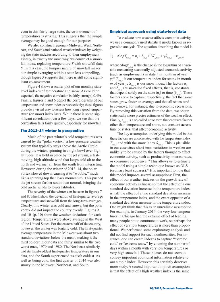
Figure 4 shows a scatter plot of our monthly state-level indexes of temperature and snow. As could be expected, the negative correlation is fairly strong (–0.49). Finally, figures 5 and 6 depict the correlograms of our temperature and snow indexes respectively; these figures provide a visual way to assess how long a good temper-ature (or snow) index lasts. While there is some sig-nificant correlation over a few days, we see that the correlation falls fairly quickly, especially for snowfall.

The 2013–14 winter in perspective

Much of the past winter’s cold temperatures was caused by the “polar vortex,” a low-pressure weather system that typically stays above the Arctic Circle during the winter, spinning in a tight bowl over high latitudes. It is held in place by the jet stream, a fast-moving, high-altitude wind that keeps cold air to the north and warmer air from the south from interacting. However, during the winter of 2013–14, the polar vortex slowed down, causing it to “wobble,” much like a spinning top that loses momentum. This pushed the jet stream farther south than normal, bringing the cold arctic winds to lower latitudes.

The severity of the winter can be seen in figures 7 and 8, which show the deviation of first-quarter average temperatures and snowfall from the long-term averages. Clearly, this winter was cold and snowy, but the polar vortex did not impact the country evenly. Figures 9 and 10 (p. 10) show the weather deviations for each region. Temperatures were above average in the West of the United States. For the eastern half of the country, however, the winter was brutally cold. The first-quarter average temperature in the Midwest was about two standard deviations below the mean, making it the third coldest in our data and fairly similar to the two worst ones, 1979 and 1980. The Northeast similarly had its third-coldest first-quarter temperature in our data, and the South experienced its sixth coldest. As well as being cold, the first quarter of 2014 was also snowy in the Midwest, Northeast, and South.

Empirical approach using state-level data

To evaluate how weather affects economic activity, we use a commonly used statistical model known as re-gression analysis. The equation describing the model is

1) ΔlogYi, m, y = αi + δm, y + βTi, m, y + γSi, m, y + εi, m, y ,

where ΔlogYi, m, y is the change in the logarithm of a vari-able measuring seasonally adjusted economic activity (such as employment) in state i in month m of year y;15 Ti, m, y is our temperature index for state i in month m of year y; Si, m, y is our snow index. The factors αi and δm, y are so-called fixed effects, that is, constants that depend solely on the state (αi ) or time (δm, y ). These factors serve to capture, respectively, the fact that some states grow faster on average and that all states tend to co-move, for instance, due to economic recessions. By removing this variation from the data, we obtain statistically more precise estimates of the weather effect. Finally, εi, m, y is a so-called error term that captures factors other than temperature and snow, not constant across time or states, that affect economic activity.

The key assumption underlying this model is that these factors are uncorrelated with the temperature index Ti, m, y and with the snow index Si, m, y. This is plausible in our case since short-term variations in weather are unlikely to be caused by the factors thought to affect economic activity, such as productivity, interest rates, or consumer confidence.16 This allows us to estimate the model using a simple technique known as OLS (ordinary least squares).17 It is important to note that this model imposes several assumptions: First, the effect of our weather indexes on the growth rate of economic activity is linear, so that the effect of a one standard deviation increase in the temperature index is half the effect of a two standard deviation increase in the temperature index, and the exact opposite of a standard deviation increase in the temperature index. One might think that this is an unrealistic assumption. For example, in January 2014, the very low tempera-tures in Chicago had the extreme effect of leading many people not to commute to work, so perhaps the effect of very low temperatures is more than propor-tional. We performed some exploratory analysis and did not find support for such nonlinearities. For in-stance, one can create indexes to capture “extreme cold” or “extreme snow” by counting the number of days within a month with very low temperatures or very high snowfall. These indexes do not seem to convey important additional information relative to our simple index. However, this certainly deserves more study. A second important implicit assumption is that the effect of a high weather index is the same


FIGURE 3

Snowfall in all stations in Illinois

Source: National Climatic Data Center.

inches

Jan. 1, 2014 Jan. 8, 2014 Jan. 15, 2014 Jan. 22, 2014 Jan. 29, 2014

30

20

10

0

FIGURE 4

Correlation between temperature and snow (winter months)

Source: Authors’ calculations based on data from the National Climatic Data Center.

snow index

−4 −2 0 2 4

temperature index

10

5

0

–5


FIGURE 5

Correlogram of temperature index


autocorrelation

0.00

0.20

0.40

0.60

0.80

0 5 10 15 20

days

FIGURE 6

Correlogram of snowfall index


autocorrelation

0.00

0.10

0.20

0.30

0.40

0 5 10 15 20

days


FIGURE 7

National temperature deviation from 1950–2014 average


degrees Fahrenheit

−5

0

5

1950 1970 1990 2010year

FIGURE 8

National snowfall deviation from 1950–2014 average


inches

−.10

−.05

0

.05

.10

.15

1950 1970 1990 2010year


FIGURE 9

Regional temperature index for first quarter


FIGURE 10

Regional snow index for first quarter


10

5

0

−5

−10

1950 1970 1990 2010year

A. Midwest temperature

Fahrenheit degrees

1950 1970 1990 2010year

B. Northeast temperatureFahrenheit degrees

1950 1970 1990 2010year

C. South temperatureFahrenheit degrees

1950 1970 1990 2010year

D. West temperatureFahrenheit degrees

−5

0

5

10

−4

−2

0

2

4

−6

−2

0

2

4

−4

Deviation from 1950–2014 average

1950 1970 1990 2010year

A. Midwest Snow Index

inches

1950 1970 1990 2010year

B. Northeast Snow Indexinches

1950 1970 1990 2010year

C. South Snow Indexinches

−.1

0

.1

.2

.3

1950 1970 1990 2010year

D. West Snow Indexinches

−.1

0

.1

.2

.3

−.2−.1

0

.1

.2

−.05

0

.05

.10

Deviation from 1950–2014 average


in all states. As we discussed above, our weather in-dexes are normalized to have the same standard devi-ation in all states, which makes this assumption more plausible, but it also deserves more study. A third as-sumption is that the average weather during the month is the relevant metric; for instance, we do not differentiate bad weather during the week from bad weather during the weekend.

Equation 1 estimates the effect of a given month’s weather on the same month’s economic vari-able Y. An important question is how long these ef-fects last. To answer this question, we also estimate the same model, but allowing for lags in the weather:

20 0

) log , , , , , , ,

, ,

∆ = + + +

+=

− −=

∑ ∑Y T Si m y i m y kk

K

i m k y k i m k yk

K

i m

α δ β γ

ε yy ,

that is, the weather in the previous K months may affect Y. This specification allows us to evaluate the strength and speed of the bounceback from a bad weather spell.18 The coefficient β0 measures the effect in a given month of a one standard deviation change in the temperature index that month, the coefficient β1 is the effect the following month, and so on.

Finally, note that we estimate this equation using the “cold season” only. That is, we define the temper-ature and snowfall indexes for November through March only (and allow the lags to work through until K months later). While weather affects the economy in the sum-mer as well, the effects are likely to be different—for instance, high temperatures might have negative effects rather than positive effects and rainfall rather than snow-fall might be relevant. This requires a different model.

Our analysis requires us to measure economic activi-ty at the state level and at high frequency. Unfortunately, there is a relative paucity of economic data at this level of regional disaggregation and at this frequency. The main source of our data is the Bureau of Labor Statis-tics’ Current Establishment Survey (CES), which sur-veys a large number of establishments each month regarding how many employees are on the payroll (during the pay period of the week including the 12th of the month). The headline national number (“nonfarm payrolls”) is released the first Friday of the following month to considerable attention, but the same survey also produces monthly estimates of employment in each state and in each industry. These are our main sources of data. We also use monthly data on new unemployment insurance claims, housing starts, and housing permits.19 Finally, we exclude Alaska and Hawaii from our analysis given their distinctive weather patterns and small population.

Results using state-level data

We first present the immediate effect of the weather, then discuss the bounceback. Finally, we study whether the economy has become less sensitive to weather over time.

Immediate effectTable 1 presents the estimates of equation 1, which

shows the effects of temperature and snowfall on total nonfarm employment, the unemployment rate, new unemployment insurance claims, housing permits, and housing starts. (Note that the economic data become available in different years, depending on the specific statistic.) A one standard deviation increase in the

TABLE 1

Nonfarm Unemployment U.I. new Housing Housing payrolls rate claims permits starts

Temperature 0.041*** – 0.034 – 0.967*** 1.124* 2.431*** (0.008) (0.253) (0.260) (0.648) (0.889)

Snowfall – 0.029*** 0.100 0.861*** – 2.091*** –1.905*** (0.006) (0.153) (0.191) (0.451) (0.595)

Observations 37,154 22,517 25,084 19,900 25,660R2 0.262 0.451 0.148 0.118 0.098Sample start 1950 1976 1971 1980 1970

Notes: Results from estimation of equation 1 using monthly data from November through March by ordinary least squares with state and time effects; standard errors in parentheses are two-way clustered by state and time. The left-hand-side variables are all in log changes, except the unemployment rate, which is in level change. Sample start date as shown; end date is 2014 for all series. U.I. indicates unemployment insurance. Temperature and snowfall indexes are normalized to have mean zero and standard deviation one for each state. Asterisks indicate statistical significance at the 10 percent (*), 5 percent (**), and 1 percent (***) level.Source: Authors’ calculations based on data from the National Climatic Data Center.

Effect of temperature and snowfall indexes on state-level economic activity


TABLE 2

Effect of temperature and snowfall on the subcomponents of state-level nonfarm employment

Temperature Snowfall Observations R2

Private nonfarm payrolls (A+B) 0.024*** (0.007) – 0.031*** (0.006) 14,143 0.426A. Goods 0.080*** (0.016) – 0.056*** (0.014) 14,143 0.3391. Mining – 0.016 (0.108) – 0.149* (0.084) 12,067 0.0582. Construction 0.185*** (0.045) – 0.181*** (0.032) 13,377 0.2733. Manufacturing 0.036** (0.016) 0.001 (0.011) 13,828 0.2353a. Durable manufacturing – 0.077 (0.132) – 0.093 (0.096) 12,226 0.9503b. Nondurable manufacturing – 0.003 (0.014) 0.004 (0.014) 13,257 0.125B. Private services 0.009 (0.006) – 0.025*** (0.006) 14,143 0.353B1. Trade, transportation, and utilities 0 (0.008) – 0.024*** (0.008) 14,143 0.322B1a. Wholesale 0.011 (0.012) – 0.015 (0.011) 13,545 0.165B1b. Retail – 0.003 (0.010) – 0.033*** (0.010) 14,143 0.259B1c. Transportation and utilities 0.005 (0.018) – 0.003 (0.014) 13,848 0.184B2. Information 0.013 (0.021) 0.021 (0.013) 12,679 0.126B3. Financial services 0.017 (0.012) 0.001 (0.011) 14,143 0.142B4. Professional and business services 0.003 (0.019) – 0.014 (0.016) 14,143 0.213B5. Education and health 0.009 (0.008) – 0.022*** (0.008) 14,143 0.092B6. Leisure and hospitality 0.041** (0.016) – 0.067*** (0.014) 14,143 0.148B6a. Accommodation and food 0.043*** (0.016) – 0.062*** (0.014) 13,839 0.146B6b. Arts and leisure 0.054 (0.045) – 0.079 (0.051) 13,388 0.066B7. Other services – 0.019 (0.013) – 0.043*** (0.012) 14,143 0.069C. Total government 0.026** (0.011) – 0.015 (0.010) 14,143 0.133C1. Federal government 0.007 (0.030) – 0.010 (0.016) 13,393 0.624C2. State government – 0.007 (0.016) – 0.030 (0.022) 13,819 0.027C3. Local government 0.040*** (0.015) – 0.021 (0.014) 13,963 0.061

Notes: Results from estimation of equation 1 using monthly data from November through March by ordinary least squares with state and time effects; standard errors in parentheses are two-way clustered by state and time. All left-hand-side variables are in log changes. Sample is 1990–2014. Temperature and snowfall indexes are normalized to have mean zero and standard deviation one for each state. Asterisks indicate statistical significance at the 10 percent (*), 5 percent (**), and 1 percent (***) level.Source: Authors’ calculations based on data from the National Climatic Data Center.

temperature index during the winter leads nonfarm employment to grow by 0.04 percent, while a one standard deviation increase in the snowfall index leads to a decline of 0.03 percent. While these percentages are small, they can be important relative to the usual month-to-month fluctuations. For example, nonfarm payrolls are around 140 million nationwide, so the 0.04 percent estimated effect of temperature amounts to a difference of around 56,000 employees, which can make the difference between a “good” labor report and an “average” one. Importantly, the effects here are highly statistically significant, but the precision of the estimate is not extremely high. This may reflect the complexity of measuring the weather accurately.

The effect on the unemployment rate has the ex-pected sign: A one standard deviation increase in the temperature index lowers the unemployment rate by 0.03 percentage points, and a one standard deviation increase in the snowfall index increases the unemploy-ment rate by one-tenth of a percentage point (for in-stance, the unemployment rate would go from 5.8 to 5.9 percentage points). However, these effects are not

statistically significant. The effects on new unemploy-ment insurance claims, housing permits, and housing starts are all highly significant, of the expected sign, and fairly large: A one standard deviation shock to either snowfall or temperature moves new claims by about 1 percent and housing starts and permits by 1–2 percent. These are larger effects, but the underlying series are also more volatile, so that a percentage point difference is not extremely important.

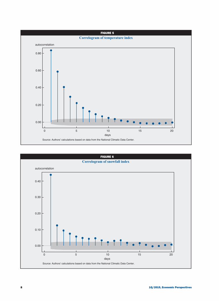
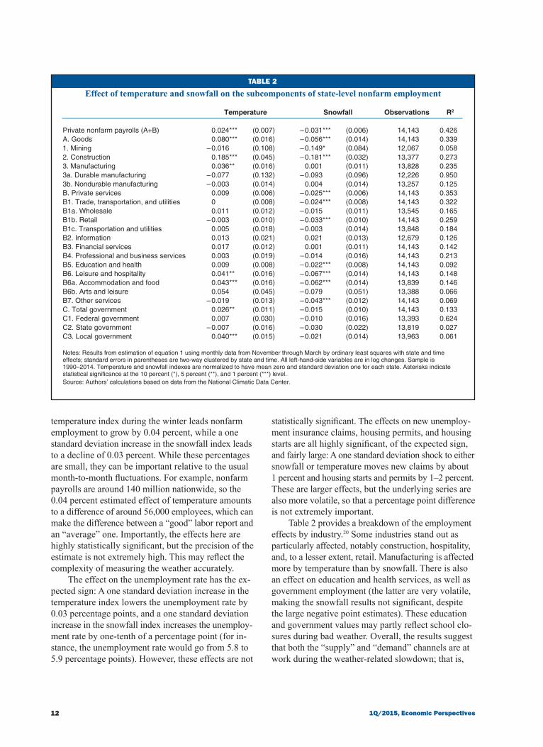
Table 2 provides a breakdown of the employment effects by industry.20 Some industries stand out as particularly affected, notably construction, hospitality, and, to a lesser extent, retail. Manufacturing is affected more by temperature than by snowfall. There is also an effect on education and health services, as well as government employment (the latter are very volatile, making the snowfall results not significant, despite the large negative point estimates). These education and government values may partly reflect school clo-sures during bad weather. Overall, the results suggest that both the “supply” and “demand” channels are at work during the weather-related slowdown; that is,


some sectors contract because it is impossible to pro-duce, while some contract because there is less demand for their services.

Beyond showing the mechanics of the weather effect, these industry responses are useful because they allow us to identify episodes in which the weather may be an important driver of the economy. Thus, if a slow-down is associated with a large decline in construction, hospitality, and retail, it may in fact be weather relat-ed (even if the weather is not well measured).

BouncebackTo evaluate how long the effects of weather last,

we estimate equation 2 with three lags (K = 3). These results are in table 3. The same-month impact effect of weather is obtained for each economic time series in the row k = 0 for temperature and snowfall, respec-tively. These are very similar to the effects found in table 1.21 The novel result in this table is that last month’s weather typically affects these economic time series with the opposite sign. For instance, a higher temper-ature index pushes nonfarm employment up by 0.043 percent the first month, but this recedes by 0.009 per-cent the next month and 0.025 percent the following month. This means that after two months, the effect of a higher temperature has largely receded. This pattern is very general across all time series, suggesting a strong bounceback, such that the level of economic activity returns roughly to where it was before the weather. A formal test of the hypothesis that a temperature shock has no effect on the level of economic activity three months later can be formulated as k

Kk= =∑ 0 0β ; and

for snowfall the test is kK

k= =∑ 0 0γ . This amounts to a test of whether the weather only has transitory effects. For all of the series studied here, we cannot reject the hypothesis that weather has only transitory effects.22 Overall, our results strongly support the intuitive notion of a bounceback.23 The bounceback usually happens within a month or two, though in at least one case (nonfarm employment) there appears to be some re-maining bounceback three months later.

Has the weather sensitivity declined?The U.S. economy has changed in many ways since

the 1960s and 1970s. New technologies for home-building have been developed, just-in-time inventory systems have been introduced, and there has been a shift away from industry and toward services. It is possible that as a result of these changes, the weather has less of an impact on the economy now than it once had. To evaluate this hypothesis, we estimate separate-ly the effects of both temperature and snow on two subsamples: prior to 1990 and after 1990.24 Table 4

reports these results. The temperature sensitivity of nonfarm employment, unemployment insurance claims, and housing permits and starts appears to have declined, though not all these changes are statistically significant. However, the snowfall sensitivity appears to have re-mained constant (for nonfarm employment) and may be even larger (for permits and starts). These last re-sults could be due to structural changes in the home-building industry, such as the lengthening of the homebuilding season.

Methodology and results using national data

In this section, we present our results using national data. The main advantage of using national data is that there are many more economic data series available at a monthly frequency at the national rather than state level. The key disadvantage, which will become ob-vious as we proceed, is that by discarding regional variation in the weather, we have less data available, which does not allow as precise estimates of the weather effect. In part, this reflects the difficulty of disentan-gling the effects of snowfall and temperature, which are strongly negatively correlated (–0.60) in our na-tional data.

Our methodology here is similar to our state-level work. We first construct a national temperature index and a national snowfall index by weighting the state indexes using nonfarm employment:

T Tm y i m y i m yi

, , , , ,==∑ω1

48

,

where ωi,m, y is the share of national nonfarm employ-ment in state i in month m of year y; and similarly for snowfall. We then run a simple time-series regression of an economic indicator on our national weather indexes:

3) ΔlogYm, y = α + βTm, y + γSm, y + εm, y ,

and later on allow for lags to capture the bounceback:

4) ∆ log ., , , ,Y T Sm y k m k y k m k yk

K

m yk

K

= + + +− −==∑∑α β γ ε00

Table 5 presents the results. Overall, there are fewer statistically significant results, and often the temperature coefficient β has the “wrong” sign. For instance, the effect of snowfall on nonfarm employ-ment is negative, but so is the temperature effect, so that this equation predicts that lower temperatures lead to higher employment. Both effects are statisti-cally insignificant. This pattern is fairly general, though in the cases of industries or activities that are


TABLE 4

Effect of temperature and snowfall on measures of state-level economic activity, pre- and post-1990

Nonfarm Unemployment U.I. Housing Housing employment rate claims permits starts

Temperature, pre-1990 0.050*** –0.588 –1.369*** 1.227 4.207*** (0.011) (0.373) (0.359) (1.371) (1.350)

Temperature, post-1990 0.023*** 0.374 –0.580* 1.049* 0.618 (0.006) (0.325) (0.341) (0.619) (0.974)

Snowfall, pre-1990 –0.030*** 0.056 0.663** –0.987 –0.379 (0.008) (0.219) (0.261) (0.870) (0.745)

Snowfall, post-1990 –0.026*** 0.143 1.069*** –2.650*** –3.563*** (0.006) (0.214) (0.261) (0.632) (1.062)

Observations 37,154 22,517 25,084 19,900 25,660R2 0.262 0.451 0.148 0.118 0.099

Notes: Results from estimation of equation 1 using monthly data from November through March by ordinary least squares with state and time effects; standard errors in parentheses are two-way clustered by state and time. The left-hand-side variables are all in log changes, except the unemployment rate, which is in level change. U.I. indicates unemployment insurance. Temperature and snowfall indexes are normalized to have mean zero and standard deviation one for each state and are interacted with two dummies, pre- and post- 1990. Asterisks indicate statistical significance at the 10 percent (*), 5 percent (**), and 1 percent (***) level.Source: Authors’ calculations based on data from the National Climatic Data Center.

TABLE 3

Effect of temperature and snowfall on state-level economic indicators with lags

Nonfarm Unemployment U.I. new Housing Housing Lag employment rate claims permits starts

Temperature Current month (k = 0) 0.043*** – 0.011 – 1.269*** 1.568*** 3.128*** (0.007) (0.247) (0.280) (0.683) (0.915)

Last month (k = 1) – 0.009 – 0.065 1.357*** – 1.577** – 3.120*** (0.007) (0.262) (0.347) (0.724) (0.888)

Two months ago (k = 2) – 0.025*** 0.174 – 0.053 – 1.111*** – 0.239 (0.008) (0.232) (0.232) (0.458) (0.827)

Three months ago (k = 3) 0.006 0.104 0.109 0.033 – 0.917 (0.007) (0.216) (0.197) (0.495) (0.855)

Snowfall Current month (k = 0) – 0.027*** 0.091 0.848*** – 2.038*** – 1.891*** (0.004) (0.152) (0.189) (0.445) (0.598)

Last month (k = 1) 0.009 0.113 – 0.275 0.944* 0.693 (0.005) (0.180) (0.234) (0.516) (0.553)

Two months ago (k = 2) 0.011*** 0.104 – 0.457** 0.385 1.222* (0.006) (0.149) (0.190) (0.548) (0.665)

Three months ago (k = 3) 0.015*** – 0.103 0.008 0.483 0.255 (0.005) (0.187) (0.193) (0.330) (0.468)

Observations 36,964 22,466 25,036 19,852 25,612R2 0.294 0.449 0.152 0.120 0.101Sample start 1950 1976 1971 1980 1970

Notes: Results from estimation of equation 2 using monthly data from November through March by ordinary least squares with state and time effects; standard errors in parentheses are two-way clustered by state and time. All left-hand-side variables are in log changes except the unemployment rate, which is in difference. U.I. indicates unemployment insurance. Temperature and snowfall indexes are normalized to have mean zero and standard deviation one for each state. Asterisks indicate statistical significance at the 10 percent (*), 5 percent (**), and 1 percent (***) level.Source: Authors’ calculations based on data from the National Climatic Data Center.


TABLE 5

Effect of temperature and snowfall on national economic indicators

Temperature Snowfall Observations R2

Nonfarm employment – 0.01 (0.028) – 0.009 (0.028) 854 0.002Unemployment rate – 0.15 (0.151) – 0.16 (0.151) 791 0.000Private nonfarm employment – 0.03 (0.031) – 0.014 (0.031) 854 0.001Construction employment 0.163* (0.098) – 0.191*** (0.098) 854 0.021Retail sales (excluding cars) 0.03 (0.077) – 0.132* (0.079) 571 0.011Private average hours per worker – 0.05* (0.028) – 0.181*** (0.029) 608 0.074Industrial production (IP): Total – 0.061 (0.126) – 0.14 (0.126) 979 0.001IP: Manufacturing 0.035 (0.137) – 0.13 (0.137) 979 0.002IP: Utilities – 1.504*** (0.159) – 0.23 (0.167) 511 0.210Lightweight vehicle sales – 0.97 (0.595) – 1.407** (0.610) 572 0.009CFNAI – 0.053 (0.085) – 0.12 (0.088) 570 0.003New orders of core capital goods – 0.46 (0.442) – 1.573*** (0.450) 270 0.054Shipments of core capital goods – 0.467* (0.281) – 0.610** (0.286) 271 0.017Housing starts 0.92 (0.629) – 2.270*** (0.631) 667 0.055Housing permits 0.58 (0.480) – 0.949** (0.482) 655 0.022Purchasing Managers Index – 0.069 (0.543) 0.45 (0.543) 791 0.002

Notes: Results from estimation of equation 3 using monthly data from November through March of all years by ordinary least squares (OLS). Standard errors in parentheses are simple OLS. All left-hand-side variables are in log changes, except for the unemployment rate (in change) and CFNAI (in level). Temperature and snowfall indexes are normalized to have mean zero and standard deviation one. Asterisks indicate statistical significance at the 10 percent (*), 5 percent (**), and 1 percent (***) level.Source: Authors’ calculations based on data from the National Climatic Data Center.

heavily affected by temperature or snowfall we do obtain clear and intuitive results. For instance, the coefficients on construction employment are similar to those ob-tained at the state level (0.163 on temperature and –0.191 on snowfall, compared with 0.185 and –0.181 for state-level data). Average hours worked, retail and car sales, housing starts and permits, and shipments and order of new capital goods are all affected signifi-cantly by snowfall. In the case of utilities production, the very strong negative effect of temperature is likely not an artifact but simply reflects the higher demand for heating. This shows that some sectors of the economy react positively to cold weather. Overall, the general message is that snowfall seems better at capturing the effect of weather on the economy, but these effects are more difficult to measure using aggregate data alone.

While it is reassuring that the magnitudes of the effects are similar (where available) in both exercises, this need not be the case. For instance, if there are spill-overs across states such that bad weather in one state negatively affects economic activity in another state, and if the weather is positively correlated across the two states, our state-level regression would overesti-mate the effect of local weather. However, these spill-overs are likely to be small.

Table 6 studies the bounceback in the national data by adding lags to equation 3. As in the state-level data, we find significant evidence of bounceback for the categories that are highly affected by temperature

or snowfall. For instance, snowfall is estimated to re-duce car sales by 1.3 percent on impact, but the bounce-back is estimated to be 1.27 percent the next month. Similarly, average hours fall by 0.17 percent then re-bound by 0.13 percent the next month. In many cases, however, the bounceback is estimated imprecisely, prob-ably due to sparseness of data at the national level.

Revisiting the 2013–14 weather contribution

We are finally in a position to estimate the effect of the 2013–14 winter on economic activity. We present two sets of results—the first one based on the national model of the previous section and the second based on the state-level model. In all cases, we simply use the actual weather observed during the winter, together with the sensitivities estimated using historical data (that is, our estimates of β and γ), to obtain the effect of the observed weather on the growth rates of these economic indicators. Table 7 presents the results based on the state-level model (which is more precisely estimated), while table 8 (p. 18) shows the national results.25 In the first row of table 7, we see that nonfarm employment dis-plays the slowdown presented in figure 1 (p. 2): Employ-ment growth rates of 0.06 percent in December and 0.1 percent in January were below the recent trend of about 0.16 percent (that is, 200,000 jobs created per month). The second row shows that, according to our estimates, the weather contributed negatively to the growth rate of nonfarm employment from November


TA

BLE

6

Eff

ect o

f tem

pera

ture

and

snow

fall

on n

atio

nal e

cono

mic

indi

cato

rs w

ith la

gs

T

emp

erat

ure

S

no

wfa

ll

Tw

o m

on

ths

C

urr

ent

mo

nth

L

ast

mo

nth

T

wo

mo

nth

s ag

o

Cu

rren

t m

on

th

Las

t m

on

th

ago

Non

farm

em

ploy

men

t –

0.00

2

(0.0

28)

–0

.033

(0

.028

)

0.01

1

(0.0

27)

–0.

011

(0

.027

) 0

.011

(0

.027

)

0.02

7 U

nem

ploy

men

t rat

e

– 0.

12

(0.1

52)

0.

25

(0.1

52)

–

0.21

(0

.150

)

– 0.

12

(0.1

50)

0.

19

(0.1

51)

–

0.21

P

rivat

e no

nfar

m e

mpl

oym

ent

0.00

4

(0.0

31)

–

0.04

3

(0.0

31)

0.

005

(0

.030

)

– 0.

016

(0

.030

)

0.00

2

(0.0

30)

0.

032

Con

stru

ctio

n em

ploy

men

t 0.

193*

*

(0.0

92)

–

0.25

2***

(0

.092

)

– 0.

082

(0

.090

)

– 0.

217*

*

(0.0

91)

–

0.01

7

(0.0

91)

0.

264*

**

Ret

ail s

ales

(ex

clud

ing

cars

)

0.09

4

(0.0

78)

–

0.10

(0

.078

)

– 0.

011

(0

.077

)

– 0.

12

(0.0

79)

0.

194*

*

(0.0

80)

–

0.01

5 P

rivat

e av

erag

e ho

urs

per

wor

ker

–

0.0

14

(0.0

28)

–

0.04

4

(0.0

28)

0.

034

(0

.027

)

– 0.

170*

**

(0.0

28)

0.

126*

**

(0.0

28)

0.

008

Indu

stria

l pro

duct

ion

(IP

): T

otal

–

0.06

3

(0.1

20)

–

0.06

1

(0.1

20)

0.

037

(0

.118

)

– 0.

15

(0.1

18)

0.

047

(0

.119

)

– 0.

003

IP: M

anuf

actu

ring

0.

037

(0

.130

)

– 0.

087

(0

.130

)

– 0.

006

(0

.128

)

– 0.

14

(0.1

28)

0.

050

(0

.129

)

– 0.

004

IP: U

tiliti

es

– 1.

636*

**

(0.1

45)

0.

906*

**

(0.1

46)

0.

536*

**

(0.1

43)

–

0.11

(0

.152

)

0.09

4

(0.1

52)

–

0.24

Li

ghtw

eigh

t veh

icle

sal

es

– 0.

62

(0.6

05)

–

0.23

(0

.606

)

0.00

1

(0.5

96)

–

1.30

3**

(0

.613

)

1.27

4**

(0

.621

)

– 0.

051

New

ord

ers

of c

ore

capi

tal g

oods

–

0.01

4

(0.0

87)

0.0

23

(0.0

87)

0.

097

(0

.086

)

– 0.

11

(0.0

88)

0.

179*

*

(0.0

89)

0.

15

New

ord

ers

of c

ore

capi

tal g

oods

–

0.34

(0

.446

)

0.19

(0

.464

)

– 0.

032

(0

.462

)

– 1.

621*

**

(0.4

67)

0.

69

(0.4

67)

0.

46

Shi

pmen

ts o

f cor

e ca

pita

l goo

ds

– 0.

522*

(0

.283

)

0.11

(0

.295

)

0.60

8**

(0

.294

)

– 0.

659*

*

(0.2

97)

0.

056

(0

.296

)

0.62

4**

Hou

sing

sta

rts

1.

345*

*

(0.6

20)

–

1.78

3***

(0

.621

)

0.28

(0

.610

)

– 2.

375*

**

(0.6

16)

0.

87

(0.6

20)

1.

846*

**

Hou

sing

per

mits

0.

70

(0.4

75)

–

1.57

8***

(0

.476

)

1.23

9***

(0

.470

)

– 1.

114*

*

(0.4

72)

–

0.18

(0

.475

)

2.00

4***

P

urch

asin

g M

anag

ers

Inde

x

– 0.

096

(0

.552

)

– 0.

036

(0

.553

)

– 0.

035

(0

.543

)

0.42

(0

.544

)

0.18

(0

.548

)

0.08

7

Not

es: R

esul

ts fr

om e

stim

atio

n of

equ

atio

n 4

usin

g m

onth

ly d

ata

from

Nov

embe

r th

roug

h M

arch

of a

ll ye

ars

by o

rdin

ary

leas

t squ

ares

(O

LS).

Sim

ple

OLS

sta

ndar

d er

rors

are

rep

orte

d in

par

enth

eses

. All

left-

hand

-si

de v

aria

bles

are

in lo

g ch

ange

s, e

xcep

t for

the

unem

ploy

men

t rat

e (in

cha

nge)

and

CF

NA

I (in

leve

l). T

empe

ratu

re a

nd s

now

fall

inde

xes

are

norm

aliz

ed to

hav

e m

ean

zero

and

sta

ndar

d de

viat

ion

one.

Ast

eris

ks

indi

cate

sta

tistic

al s

igni

fican

ce a

t the

10

perc

ent (

*), 5

per

cent

(**

), a

nd 1

per

cent

(**

*) le

vel.

Sou

rce:

Aut

hors

’ cal

cula

tions

bas

ed o

n da

ta fr

om th

e N

atio

nal C

limat

ic D

ata

Cen

ter.


TABLE 7

Estimated effect of 2013–14 winter using state model

Nov. Dec. Jan. Feb. Mar. Apr. May

Nonfarm employment Data 0.20 0.06 0.10 0.16 0.15 0.22 0.17 Weather effect – 0.02 – 0.02 – 0.01 – 0.04 0.00 0.03 0.03Unemployment rate Data – 0.20 – 0.30 – 0.10 0.10 0.00 – 0.40 0.00 Weather effect – 0.02 0.03 – 0.05 0.06 0.03 – 0.03 – 0.27New unemployment Data – 5.30 8.27 – 9.27 5.43 – 3.26 – 2.29 – 0.83 insurance claims Weather effect 0.24 0.22 – 0.07 0.98 – 0.31 – 1.13 0.08Housing permits Data – 2.85 – 1.46 – 8.47 7.39 – 1.09 5.73 – 5.23 Weather effect – 0.59 – 0.32 0.95 – 1.04 1.11 1.51 1.08Housing starts Data 16.60 – 6.64 – 14.21 3.40 2.34 11.24 – 7.72 Weather effect – 1.71 – 0.27 0.85 – 0.67 0.22 3.35 0.62

Notes: Based on state model with three lags. All results are in percentage growth rates, except for the unemployment rate, which is the change in percentage points.Source: Authors’ calculations based on data from the National Climatic Data Center.

through February, to the tune of 0.04 percent in Feb-ruary, or about 50,000 to 60,000 jobs. The weather effects are then reversed in April and May. However, the weather hardly accounts for the weak December and January employment numbers. Similarly, the un-employment rate grew by 0.06 percentage points in February due to weather, according to these estimates. Housing permits and starts were also affected in a signif-icant way, but the estimated effects (about 1 percent) fall short of the observed magnitude of the decline in the data (14 percent for starts and 8 percent for permits in January, for instance).

In table 8, we see that the results with national data have the same flavor, but are less clear perhaps due to the imprecision of the estimation. For instance, the weather effect is now estimated to be positive for nonfarm employment during most months. However, this relies on an equation that was insignificant. More sensible results are obtained for construction employ-ment, retail sales, average hours worked, and lightweight vehicle sales. For instance, hours fell 0.6 percent in February, of which 0.19 percent is attributed to the weather. Utility production grew 3.3 percent in January, of which 0.52 percent is attributed to the weather. The decline in starts and permits due to weather is about 3 percent. However, the timing does not fit the observed decline in indicators well. For instance, the CFNAI fell sharply in January, and our model attributes little of this to the weather; and housing starts and permits rebounded in February, contrary to our model’s pre-diction. Overall, while some of the patterns observed in the data can be attributed in part to weather, this explanation is insufficient to explain the magnitude and timing of the slowdown.

How does climate change affect our results?

It is important to note the potential impact of cli-mate change on our study. When we construct our weather index, we normalize by a base value, which we take to be simply the long-run average (1950–2014). However, it is conceivable that given rising global temperatures, the typical temperature in the United States increased during the period of observation. This would make, for example, a 25-degree day in November more anomalous in 2014 than in 1950. As noted above, our weather data are not adjusted for changes in in-strumentation and other measurement issues. Without these adjustments, it is difficult to detect a trend in temperature.26 However, in some cases it is possible to observe a positive trend starting in 1980, which is consistent with the evidence on climate change on the United States. To assess the effect of this potential trend on our results, we fitted a linear trend starting in 1980 to each weather index and reestimated our models. All of our results are nearly unaffected by this modifi-cation. This is not surprising since the effect of weather is intuitively identified using the short-run deviations of weather, which are much larger than the trend. In-corporating the trend has one significant consequence: It makes the 2013–14 winter look even harsher; that is, the weather deviation from normal is larger due to the positive trend. This implies that our estimated effect of that winter weather is larger, by about 20 percent, than we discussed in the previous section.

Conclusion

Our results overall support the view that weather has a significant, but short-lived, effect on economic activity. Except for a few industries, which are affected importantly (such as utilities, construction, hospitality,


TABLE 8

Estimated effect of 2013–14 winter using national model

Nov. Dec. Jan. Feb. Mar. Apr. May

Nonfarm employment Data 0.20 0.06 0.10 0.16 0.15 0.22 0.17 Weather effect 0.01 0.02 – 0.01 0.02 0.07 0.08 – 0.02Unemployment rate Data – 0.20 – 0.30 – 0.10 0.10 0.00 – 0.40 0.00 Weather effect 0.16 – 0.31 0.25 – 0.19 0.31 – 0.57 0.29Retail sales (excluding cars) Data – 0.38 0.55 – 0.47 0.36 0.81 0.72 0.25 Weather effect – 0.02 – 0.11 – 0.02 – 0.07 0.35 0.09 0.02Private average hours per worker Data 0.30 – 0.60 0.30 – 0.60 0.89 0.00 0.00 Weather effect 0.09 – 0.10 – 0.08 – 0.19 0.30 0.03 – 0.04Industrial production (IP) Data 0.59 0.20 – 0.30 0.98 0.78 0.10 0.48 Weather effect 0.12 – 0.02 – 0.06 – 0.17 0.21 0.03 – 0.05IP: Manufacturing Data 0.31 0.10 – 0.93 1.23 0.81 0.30 0.40 Weather effect 0.04 – 0.04 – 0.08 – 0.20 0.14 0.10 0.01IP: Utilities Data 1.85 0.10 3.32 – 0.28 – 0.47 – 5.30 0.20 Weather effect 1.39 – 0.14 0.52 0.15 0.88 – 2.05 – 0.65Lightweight vehicle sales Data 5.79 – 4.74 – 1.60 0.90 6.88 – 2.81 4.29 Weather effect 1.11 – 0.79 0.13 – 0.77 3.54 0.05 0.00CFNAI Data 0.71 – 0.19 – 0.85 0.55 0.53 0.15 0.18 Weather effect 0.06 – 0.15 – 0.15 – 0.03 0.41 0.15 – 0.14New orders on core capital goods Data 5.72 – 0.88 – 1.90 0.10 4.58 – 1.10 – 1.41 Weather effect 1.03 – 1.15 – 1.05 – 2.18 2.21 0.60 – 0.01Shipments of core capital goods Data 2.81 0.38 – 1.91 0.83 2.16 – 0.31 0.08 Weather effect 0.73 – 0.23 – 0.97 – 0.84 0.81 0.57 – 0.83Housing starts Data 16.60 – 6.64 – 14.21 3.40 2.34 11.24 – 7.72 Weather effect 0.01 – 0.72 – 2.98 – 2.77 3.10 5.50 – 0.55Housing permits Data – 2.85 – 1.46 – 8.47 7.39 – 1.09 5.73 – 5.23 Weather effect – 0.05 0.51 – 2.87 – 1.19 0.95 4.87 – 1.78Purchasing Managers Index Data 57.00 56.50 51.30 53.20 53.70 54.90 55.40 Weather effect – 0.12 0.20 0.53 1.14 0.56 0.22 0.03

Notes: Based on national model with two lags. All results are in percentage growth rates, except the unemployment rate, which is the change in percentage points. Source: Authors’ calculations based on data from the National Climatic Data Center.

and, to a lesser extent, retail), the effect is not very large, so that even the fairly bad weather during the 2013–14 winter cannot account entirely for the weak economy during that period. Other factors must have been at play. Indeed, the National Income and Product Accounts data suggest that an important share of the slowdown in the first quarter was driven by an inventory correction and the effect of foreign trade. Another simple hint that something more than the weather was at play is that the timing of the decline, measured in economic statistics in the period December through March, was uneven across indicators: Some declined in December

and January, others in January and February, and so on, which seems inconsistent with a simple weather story. There are several directions in which it would be interesting to extend this work. First, better weather indexes could be constructed by weighting station data using very local employment. The importance of nonlinearities could also be studied in more detail, as could the differences across states in sensitivities to weather. Finally, local measurement of production and sales would enable us to extend this study and consider more outcomes.


NOTES

1These indicators come from a variety of data sources, including private or government surveys, trade associations, or administrative data. These statistics are followed closely by investors because they are released often and with little lag, and hence are more timely and less subject to revisions than the broader and more comprehen-sive measures such as gross domestic product.

2FOMC statements noted starting in December 2013 that “asset purchases are not on a preset course, and the Committee’s decisions about their pace will remain contingent on the Committee’s outlook for the labor market and inflation as well as its assessment of the likely efficacy and costs of such purchases.” See www.federalreserve.gov/newsevents/press/monetary/20131218a.htm .

3Recently, there has been some renewed interest by economists in the question of how weather affects the economy, but this research was not relevant for the issues at hand, as we explain.

4The minutes from the March 2014 meeting provided more detail: “The information reviewed for the March 18–19 meeting indicated that economic growth slowed early this year, likely only in part be-cause of the temporary effects of the unusually cold and snowy winter weather. ... The staff’s assessment was that the unusually severe winter weather could account for some, but not all, of the recent unanticipated weakness in economic activity, and the staff lowered its projection for near-term output growth. ... Most participants noted that unusually severe winter weather had held down economic activ-ity during the early months of the year. Business contacts in various parts of the country reported a number of weather-induced disrup-tions, including reduced manufacturing activity due to lost work-days, interruptions to supply chains of inputs and delivery of final products, and lower-than-expected retail sales. Participants expected economic activity to pick up as the weather-related disruptions to spending and production dissipated.” See www.federalreserve.gov/monetarypolicy/fomcminutes20140319.htm.

5 See www.federalreserve.gov/mediacenter/files/FOMCpresconf20140319.pdf .

6The minutes noted that “the information reviewed for the April 29–30 meeting indicated that growth in economic activity paused in the first quarter as a whole, but that activity stepped up late in the quarter; this pattern reflected, in part, the temporary effects of the unusually cold and snowy weather earlier in the quarter and the unwinding of those effects later in the quarter.” See www.federalreserve.gov/monetarypolicy/fomcminutes20140430.htm.

7 See www.federalreserve.gov/newsevents/speech/yellen20140416a.htm.

8Published on the New York Times website September 26, 2014; available at www.nytimes.com/2014/09/27/upshot/gdp-report- emphasizes-the-problem-of-conflicting-economic-signals.html.

9See, for instance, Gallup, Sachs, and Mellinger (1999).

10The data are available at ftp://ftp.ncdc.noaa.gov/pub/data/ghcn/daily. Our data set is version 3.12, retrieved in September 2014.

11One important data issue is that until recently, snowfall was often not reported unless it was snowing; that is, the data are reported as missing rather than zero. As we believe is standard practice, we at-tribute a zero snowfall to all missing observations (which may include some observations for which no data were actually observed).

12As a result of the lack of adjustments, our data do not exhibit very clear increases in average temperature. We believe the adjust-ments, while critical for the measurement of the trend in average

temperature, are not important for the measurement of short-term weather. We discuss this in more detail in the last section.

13We calculate the daily temperature as the simple average of the minimum and maximum daily temperature, that is,

T T T=

+max min .2

14The underlying issue is whether normalizing helps capture the ef-fect of unusual weather on economic activity. We hypothesize that economies in highly variable climates have adapted: For example, states with highly variable levels of snowfall may have the infra-structure in trucks and salt to deal with large snowfall events. This is largely an empirical question. In some explorations, we found that the precise normalization was not critical to our result, but this is an area that deserves future research.

15The log change approximates the percentage change in the variable Y, while reducing the effects of outliers and heteroskedasticity.

16However, it may be that economic activity in state i depends on weather in other states, for example, because of supply chains or because lower retail sales in one state affect production in another state. Because weather may be correlated across states, this could lead to a bias.

17The error terms εi, m, y may be correlated across states and over time; we adjust the standard errors to take this into account using two-way clustering.

18Technically, this equation requires defining Ti, m–k, y = Ti, m–k+12, y–1 if m – k ≤ 0.

19We are not aware of monthly data available on sales or production at the state level.

20The breakdown of employment by industry at the state level and at the monthly frequency is only available for the period 1990–2014, so we have fewer data and consequently fewer statistically signifi-cant results. The sample size varies further by industry because the Bureau of Labor Statistics’ establishment survey does not report employment for some industries in some states.

21This is expected since our indexes of temperature and snowfall exhibit relatively little serial correlation; hence, adding lagged values to the regression does not affect the same-month impact estimates since current weather and lagged weather are roughly orthogonal.

22The only marginal case is the effect of temperature on housing permits, which is significant at the 7 percent level.

23Note, however, that the precision of the estimates does not permit us to rule out a small long-run effect.

24Technically, we interact both of our weather indexes with two dummies, pre- and post-1990, and run a single regression for each economic indicator.

25We construct the national implied weather effects from the state model by weighting the state-level predictions to adjust for the state size.

26There appears to be no trend in precipitation, even in “adjusted” data.


REFERENCES

Boldin, Michael, and Jonathan H. Wright, 2015, “Weather-adjusting employment data,” Federal Reserve Bank of Philadelphia, working paper, No. 15-05, January.

Colacito, Riccardo, Bridget Hoffman, and Toan Phan, 2014, “Temperatures and growth: A panel analysis of the U.S.,” University of North Carolina at Chapel Hill, working paper, December 18.

Dell, Melissa, Benjamin F. Jones, and Benjamin A. Olken, 2014, “What do we learn from the weather? The new climate-economy literature,” Journal of Economic Literature, Vol. 52, No. 3, September, pp. 740–798.

__________, 2012, “Temperature shocks and economic growth: Evidence from the last half century,” American Economic Journal: Macroeconomics, Vol. 4, No. 3, July, pp. 66–95.

Deryugina, Tatyana, and Solomon M. Hsiang, 2014, “Does the environment still matter? Daily temperature and income in the United States,” National Bureau of Economic Research, working paper, No. 20750, December.

Deschênes, Olivier, and Michael Greenstone, 2007, “The economic impacts of climate change: Evidence from agricultural output and random fluctuations in weather,” American Economic Review, Vol. 97, No. 1, March, pp. 354–385.

Gallup, John Luke, Jeffrey D. Sachs, and Andrew D. Mellinger, 1999, “Geography and economic development,” International Regional Science Review, Vol. 22, No. 2, August, pp. 179–232.

Macroeconomic Advisers, 2014, “Elevated snowfall reduced Q1 GDP growth 1.4 percentage points,” April 15, available at www.macroadvisers.com/2014/ 04/elevated-snowfall-reduced-q1-gdp-growth-1-4- percentage-points/.

1q2015-part1-bloesch-gourio-pdf (1)

Documents

economic indicators

economic recovery

economic research department

economic indicators

bad weather

extreme weather

variety of indicators

retail sales