2 1 (a) (b) 2, 2; ancel each...
TRANSCRIPT

, 9th Edition A Automatic Control Systems Chapter 2 Solutionns Golnarr
C
2
(
2
2
M
Chapter 2
2‐1 (a) Poles
Zeros
(c) Poles: s =
Zeros
2-2) a)
b)
c)
2-3)
MATLAB code
s: s = 0, 0, −1, −
s: s = −2, ∞, ∞
0, −1 + j, −1 −
s: s = −2.
e:
−10;
, ∞.
j;
(b)
(d) Poles: s
2‐1
Poles: s = −2,
Zeros: s = 0.
The pole and
= 0, −1, −2, ∞
, −2;
zero at s = −1 c
.
aghi, Kuo
cancel each otther.

Automatic Control Systems, 9th Edition Chapter 2 Solutions Golnaraghi, Kuo clear all;
s = tf('s')
'Generated transfer function:'
Ga=10*(s+2)/(s^2*(s+1)*(s+10))
'Poles:'
pole(Ga)
'Zeros:'
zero(Ga)
'Generated transfer function:'
Gb=10*s*(s+1)/((s+2)*(s^2+3*s+2))
'Poles:';
pole(Gb)
'Zeros:'
zero(Gb)
'Generated transfer function:'
Gc=10*(s+2)/(s*(s^2+2*s+2))
'Poles:';
pole(Gc)
'Zeros:'
zero(Gc)
'Generated transfer function:'
Gd=pade(exp(-2*s),1)/(10*s*(s+1)*(s+2))
'Poles:';
pole(Gd)
'Zeros:'
zero(Gd)
2‐2
Automatic Control Systems, 9th Edition Chapter 2 Solutions Golnaraghi, Kuo
Poles and zeros of the above functions:
(a)
Poles: 0 0 ‐10 ‐1
Zeros: ‐2
(b)
Poles: ‐2.0000 ‐2.0000 ‐1.0000
Zeros: 0 ‐1
(c)
Poles:
0
‐1.0000 + 1.0000i
‐1.0000 ‐ 1.0000i
Zeros: ‐2
Generated transfer function:
(d) using first order Pade approximation for exponential term
Poles:
0
‐2.0000
‐1.0000 + 0.0000i
‐1.0000 ‐ 0.0000i
Zeros:
1
2‐3

Automatic Control Systems, 9th Edition Chapter 2 Solutions Golnaraghi, Kuo 2-4) Mathematical re ation: present
In all cases substitute and simplify. The use MATLAB to verify.
a)
31 2
2
2
2 2 2
2 2 2 2 2
10( 2)( 1)( 10)
10( 2) ( 1)( 10)( 1)( 10) ( 1)( 10)
10( 2)( 1)( 10)( 1)( 100)2 1 10
2 1 10( )jj j
jj j
j j jj j j j
j j j
j j jR
R e e e φφ φ
ωω ω ω
ω ω ω +ω ω ω ω ω
ω ω ωω ω ωω ω ω
ω ω ω
+− + +
+ − + −= ×− + + − + − +
+ − + − +=
− + ++ − + − +
=+ + +
=
2 2 2 2 2
2 2 2
2 211
2 2
212
2
2 213
2 2
1 2 3
10 2 1 10 ;( 1)( 100)
2tan 22
1tan 11
10tan 1010
R ω ω ωω ω ω
ωωφ
ωωωφ
ωωωφ
ωφ φ φ φ
−
−
−
+ + +=
− + +
+=
+−
+=
+−
+=
+= + +
b)
31 2
2
2 2 2
2 2 2
10( 1) ( 3)
10 ( 1)( 1)( 3)( 1)( 1)( 3) ( 1)( 1)( 3)10( 1)( 1)( 3)
( 1) ( 9)1 1 3
1 1 9( )jj j
j jj j j
j j j j j jj j j
j j jR
R e e e φφ φ
ω ωω ω ω
ω ω ω ω ω ωω ω ωω ω
ω ω ωω ω ω
+ +− + − + − +
= ×+ + + − + − + − +− + − + − +
=+ +
− + − + − +=
+ + +=
2 2
2 2 2
211
2
212
2
213
2
1 2 3
10 1 9 ;( 1) ( 9)
1tan 11
1tan 11
9tan 39
R ω ωω ω
ωωφ
ωωωφ
ωωωφ
ωφ φ φ φ
−
−
−
+ +=
+ +−
+=
+−
+=
+−
+=
+= + +
2‐4

Automatic Control Systems, 9th Edition Chapter 2 Solutions Golnaraghi, Kuo
c)
2
2
2 2
2
2 2 2
2
2 2 2
10( 2 2 )
10 (2 2 )( 2 2 ) (2 2 )
10( 2 (2 ) )(4 (2 ) )
2 (2 )4 (2 )
( )j
j jj j
j jj
jR
R e φ
ω ω ωω ω
ω ω ω ωω ω
ω ω ωω ωω ω
+ −
− − −= ×
+ − − −
− − −=
+ −
− − −=
+ −
=
ω
2 2 2
2 2 2 2 2
2
2 2 21
2 2
10 4 (2 ) 10 ;(4 (2 ) ) 4 (2 )
24 (2 )tan 2
4 (2 )
Rω ω
ω ω ω ω ω ω
ωω ωφ ω
ω ω
−
+ −= =
+ − + −
− −
+ −= −
+ −
2
2
d)
31 2
2
22 2
2 /2
2 2 2
10 ( 1)( 2)( 1)( 2)
10 ( 1)( 2)2 1
2 1( )
j
j
j j
jj j
ej j jj j j e
j jR e
R e e e
ω
ω
ω π
φφ φ
ω ω ωω ω
ω ω ωω ω
ω ω
−
−
− −
+ +− − + − +
=+ +
− + − +=
+ +=
2 2 2
2 211
2 2
212
2
1 2 3
1 ;10 2 1
2tan 22
1tan 11
Rω ω ω
ωωφ
ωωωφ
ωφ φ φ φ
−
−
=+ +−
+=
+−
+=
+= + +
MATLAB code:
clear all;
s = tf('s')
'Generated transfer function:'
Ga=10*(s+2)/(s^2*(s+1)*(s+10))
figure(1)
2‐5
Automatic Control Systems, 9th Edition Chapter 2 Solutions Golnaraghi, Kuo Nyquist(Ga)
'Generated transfer function:'
Gb=10*s*(s+1)/((s+2)*(s^2+3*s+2))
figure(2)
Nyquist(Gb)
'Generated transfer function:'
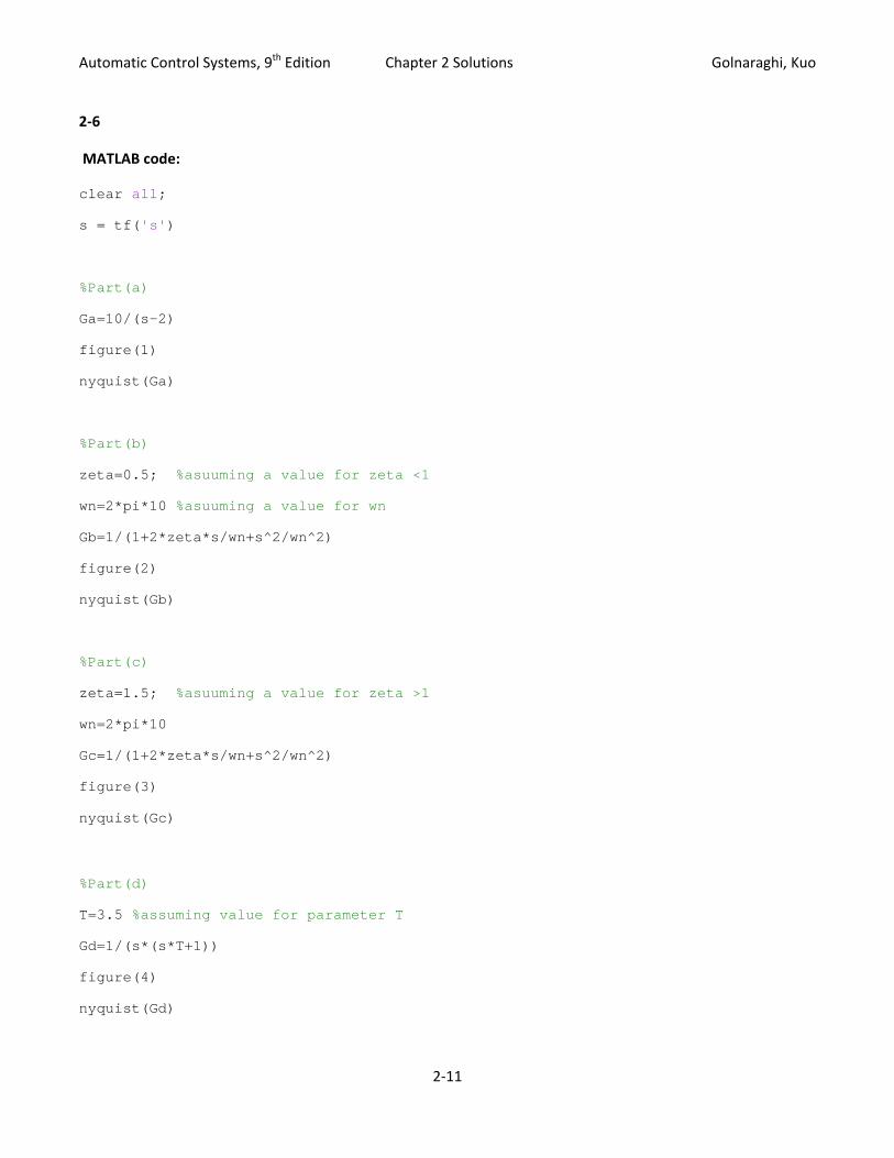
Gc=10*(s+2)/(s*(s^2+2*s+2))
figure(3)
Nyquist(Gc)
'Generated transfer function:'
Gd=pade(exp(-2*s),1)/(10*s*(s+1)*(s+2))
figure(4)
Nyquist(Gd)
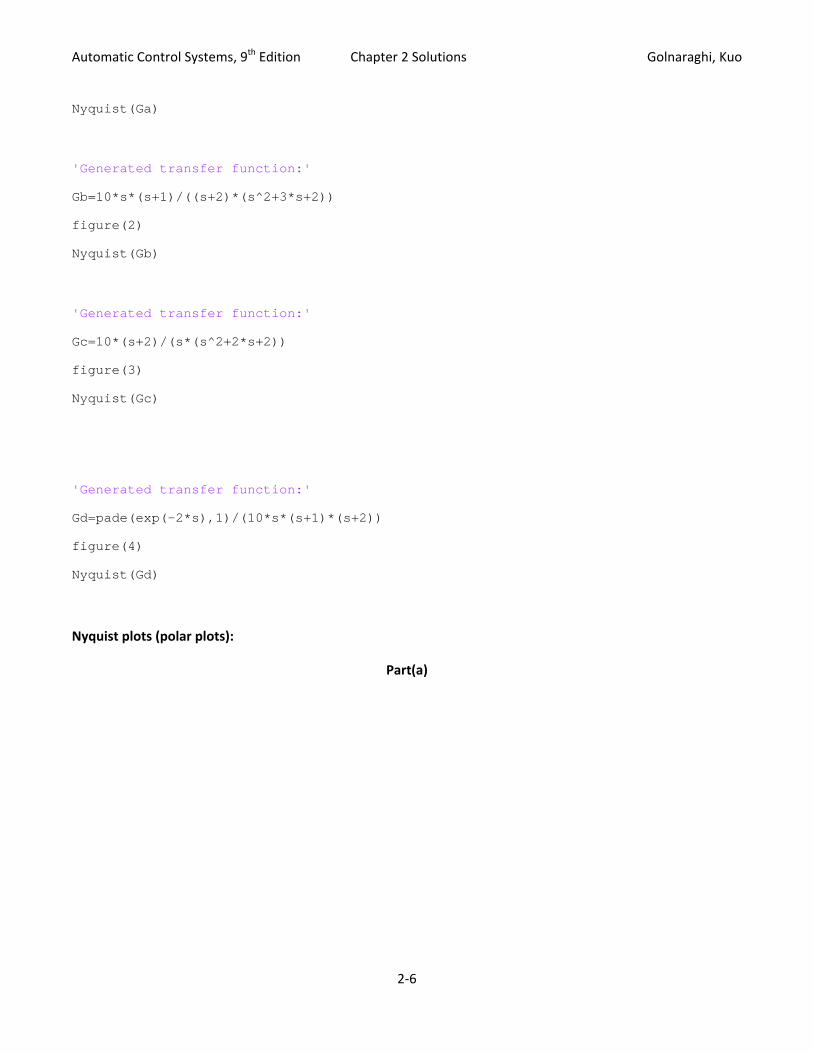
Nyquist plots (polar plots):
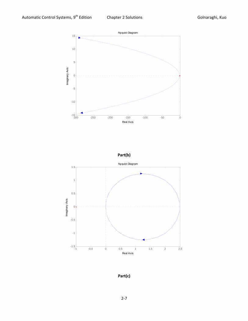
Part(a)
2‐6
Automatic Control Systems, 9th Edition Chapter 2 Solutions Golnaraghi, Kuo
-300 -250 -200 -150 -100 -50 0-15
-10
-5
0
5
10
15Nyquist Diagram
Real Axis
Imag
inar
y Ax
is
Part(b)
-1 -0.5 0 0.5 1 1.5 2 2.5-1.5
-1
-0.5
0
0.5
1
1.5Nyquist Diagram
Real Axis
Imag
inar
y Ax
is
Part(c)
2‐7

Automatic Control Systems, 9th Edition Chapter 2 Solutions Golnaraghi, Kuo
-7 -6 -5 -4 -3 -2 -1 0-80
-60
-40
-20
0
20
40
60
80Nyquist Diagram
Real Axis
Imag
inar
y Ax
is
Part(d)
-1 -0.8 -0.6 -0.4 -0.2 0 0.2 0.4-2.5
-2
-1.5
-1
-0.5
0
0.5
1
1.5
2
2.5Nyquist Diagram
Real Axis
Imag
inar
y Ax
is
2‐8
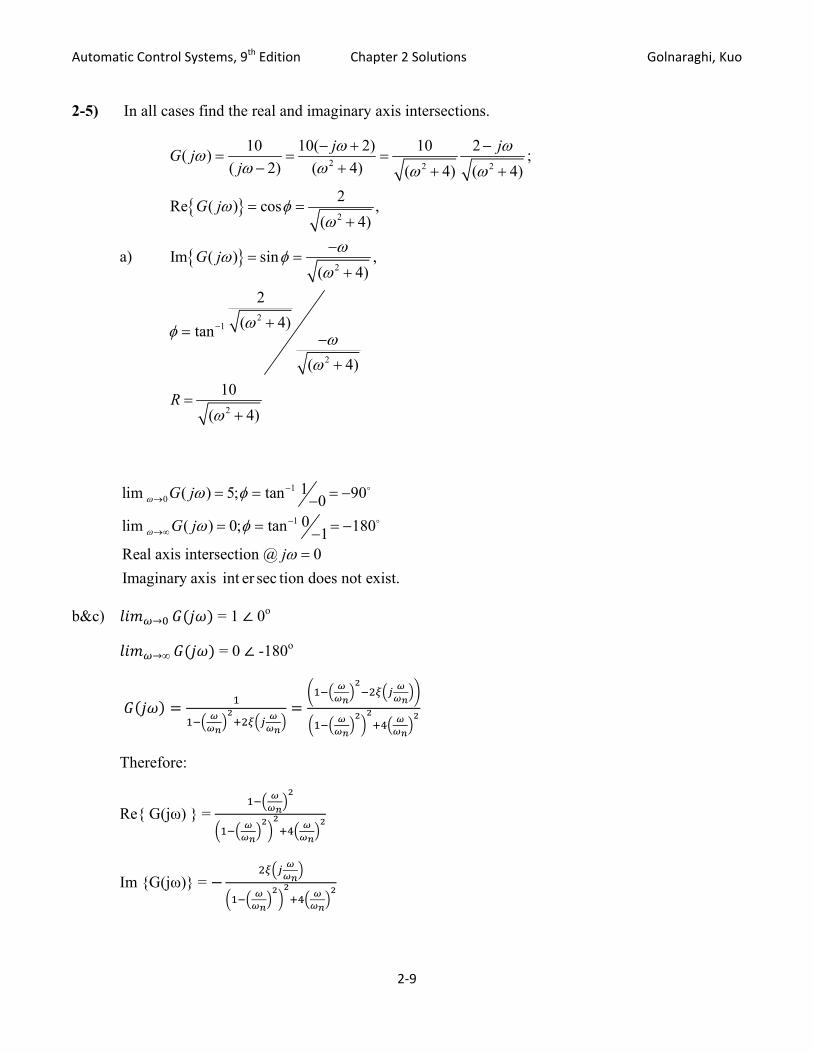
Automatic Control Systems, 9th Edition Chapter 2 Solutions Golnaraghi, Kuo 2-5) In all cases find the real and imaginary axis intersections.
a)
{ }
{ }
2 2 2
2
2
21
2
2
10 10( 2) 10 2( )( 2) ( 4) ( 4) ( 4)
2Re ( ) cos ,( 4)
Im ( ) sin ,( 4)
2( 4)tan
( 4)10
( 4)
j jG jj
G j
G j
R
;ω ωωω ω ω ω
ω φωωω φ
ω
ωφ ωω
ω
−
− + −= = =
− + + +
= =+
−= =
+
+= −
+
=+
10
1
1lim ( ) 5; tan 9000lim ( ) 0; tan 1801
Real axis intersection @ 0Imaginary axis er
b&c) = 1 o
int sec tion does not exist.
G j
G j
j
ω
ω
ω φ
ω φ
ω
−→
−→∞
= = = −−
= = = −−=
o
o
0
∞ = 0 -180o
Therefore:
Re{ G(jω) } =
Im {G(jω)} =
2‐9

Automatic Control Systems, 9th Edition Chapter 2 Solutions Golnaraghi, Kuo
If Re{G(jω )} = 0
If Im{ G(jω )} = 0 00
∞
If ω = ωn
90
If ω = ωn and ξ = 1
If ω = ωn and ξ 0
If ω = ωn and ξ ∞ 0
d) ω) =G(j
ωlim G jω =
limω ∞ G jω =
- 90o
-180o
e) || √
G(jω) = + = tan-1 (ω T) – ω L
2‐10
Automatic Control Systems, 9th Edition Chapter 2 Solutions Golnaraghi, Kuo 2‐6
MATLAB code:
clear all;
s = tf('s')
%Part(a)
Ga=10/(s-2)
figure(1)
nyquist(Ga)
%Part(b)
zeta=0.5; %asuuming a value for zeta <1
wn=2*pi*10 %asuuming a value for wn
Gb=1/(1+2*zeta*s/wn+s^2/wn^2)
figure(2)
nyquist(Gb)
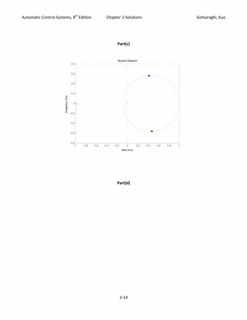
%Part(c)
zeta=1.5; %asuuming a value for zeta >1
wn=2*pi*10
Gc=1/(1+2*zeta*s/wn+s^2/wn^2)
figure(3)
nyquist(Gc)
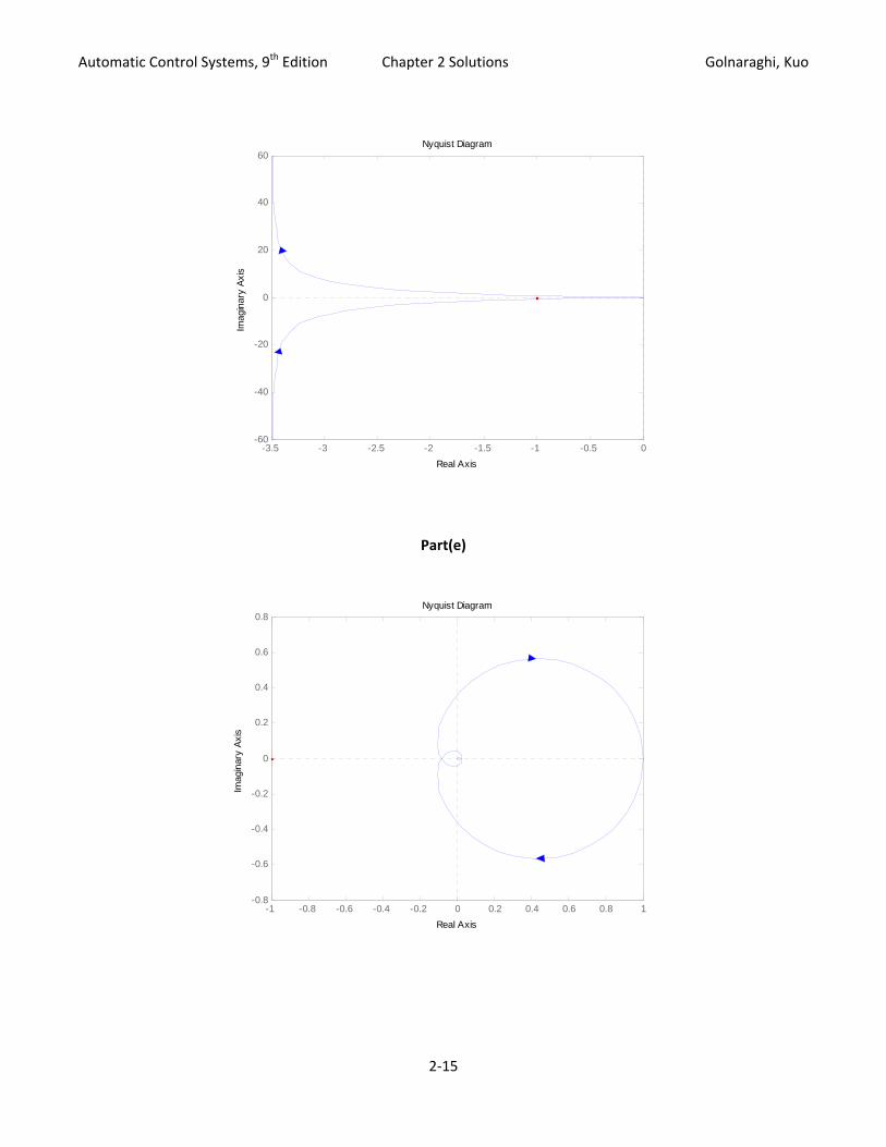
%Part(d)
T=3.5 %assuming value for parameter T
Gd=1/(s*(s*T+1))
figure(4)
nyquist(Gd)
2‐11

Automatic Control Systems, 9th Edition Chapter 2 Solutions Golnaraghi, Kuo %Part(e)
T=3.5
L=0.5
Ge=pade(exp(-1*s*L),2)/(s*T+1)
figure(5)
hold on;
nyquist(Ge)
notes: In order to use Matlab Nyquist command, parameters needs to be assigned with values, and Pade approximation needs to be used for exponential term in part (e).
Nyquist diagrams are as follows:
2‐12

Automatic Control Systems, 9th Edition Chapter 2 Solutions Golnaraghi, Kuo
Part(a)
-5 -4 -3 -2 -1 0 1-2.5
-2
-1.5
-1
-0.5
0
0.5
1
1.5
2
2.5Nyquist Diagram
Real Axis
Imag
inar
y Ax
is
Part(b)
-1 -0.8 -0.6 -0.4 -0.2 0 0.2 0.4 0.6 0.8 1-1.5
-1
-0.5
0
0.5
1
1.5Nyquist Diagram
Real Axis
Imag
inar
y Ax
is
2‐13
Automatic Control Systems, 9th Edition Chapter 2 Solutions Golnaraghi, Kuo
Part(c)
-1 -0.8 -0.6 -0.4 -0.2 0 0.2 0.4 0.6 0.8 1-0.8
-0.6
-0.4
-0.2
0
0.2
0.4
0.6
0.8Nyquist Diagram
Real Axis
Imag
inar
y Ax
is
Part(d)
2‐14
Automatic Control Systems, 9th Edition Chapter 2 Solutions Golnaraghi, Kuo
-3.5 -3 -2.5 -2 -1.5 -1 -0.5 0-60
-40
-20
0
20
40
60Nyquist Diagram
Real Axis
Imag
inar
y Ax
is
Part(e)
-1 -0.8 -0.6 -0.4 -0.2 0 0.2 0.4 0.6 0.8 1-0.8
-0.6
-0.4
-0.2
0
0.2
0.4
0.6
0.8Nyquist Diagram
Real Axis
Imag
inar
y Ax
is
2‐15

Automatic Control Systems, 9th Edition Chapter 2 Solutions Golnaraghi, Kuo
2-7) a) G(jω) =. .
Steps for plotting |G|:
(1) For ω < 0.1, asymptote is
Break point: ω = 0.5 Slope = -1 or -20 dB/decade
(2) For 0.5 < ω < 10 Break point: ω = 10 Slope = -1+1 = 0 dB/decade
(3) For 10 < ω < 50: Break point: ω = 50 Slope = -1 or -20 dB/decade
(4) For ω > 50 Slope = -2 or -40 dB/decade
Steps f r plotting G o
(1) = -90o
(2) = 0: 90
∞
0
(3) .
= 0:
. 0
. ∞:
90
(4) .
= 0:
.90
∞ .
0
b) Let’s convert the transfer function to the following form:
G(jω) = . G(s) = .
Steps for plotting |G|:
2‐16
(1) Asymptote: ω < 1 |G(jω)| 2.5 / ω Slope: -1 or -20 dB/d| | 2.5
ecade

Automatic Control Systems, 9th Edition Chapter 2 Solutions Golnaraghi, Kuo
(2) ωn =2 and ξ = 0.1 for second-order pole break point: ω = 2 slope: -3 60 d cade
| |
or - dB/ e
5
Steps for plotting G(jω):
(1) for term 1/s the phase starts at -90o and at ω = 2 the phase will be -180o (2) for higher frequencies the phase approaches -270o
c) Convert the transfer function to the following form:
0.01 1
0.01 9 1
for term , slope is -2 (-40 dB/decade) and passes through | | 1
(1) the breakpoint: ω = 1 and slope is zero (2) the breakpoint: ω = 2 and slope is -2 or -40 dB/decade
|G(jω)|ω = 1 = 2 = 0.01 below the asymptote ξ|G(jω)|ω = 1 =
. = 50 above the asymptote
ξ =
Steps for plotting G:
(1) ase starts from -180o due to ph
(2) G(jω)|ω =1 = 0 (3) G(jω)|ω = 2 = -180o
d) G(jω) = ξ ω
ωωω
Steps for plotting the |G|:
(1) Asymptote for <1 is zero
(2) Breakpoint: = 1, slope = -1 or -10 dB/decade
(3) As ξ is a damping ratio, then the magnitude must be obtained for various ξ when 0 ≤ ξ ≤ 1
2‐17

Automatic Control Systems, 9th Edition Chapter 2 Solutions Golnaraghi, Kuo
The high frequency slope is twice that of the asymptote for the single-pole case
Steps for plotting G:
(1) The phase starts at 0o and falls -1 or -20 dB/decade at = 0.2 and approaches -180o
at = 5. For > 5, the phase remains at -180o.
(2) As ξ is a damping ratio, the phase angles must be obtained for various ξ when 0 ≤ ξ ≤ 1
2‐8) Use this part to confirm the results from the previous part.
MATLAB code:
s = tf('s')
'Generated transfer function:'
Ga=2000*(s+0.5)/(s*(s+10)*(s+50))
figure(1)
bode(Ga)
grid on;
'Generated transfer function:'
Gb=25/(s*(s+2.5*s^2+10))
figure(2)
bode(Gb)
grid on;
'Generated transfer function:'
Gc=(s+100*s^2+100)/(s^2*(s+25*s^2+100))
figure(3)
bode(Gc)
grid on;
2‐18
Automatic Control Systems, 9th Edition Chapter 2 Solutions Golnaraghi, Kuo
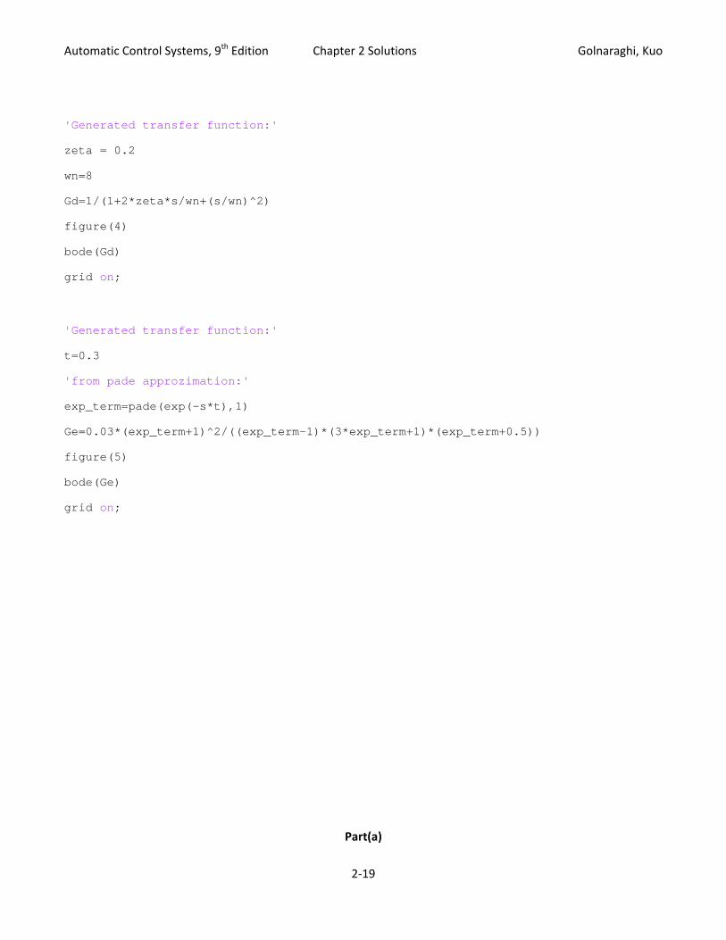
'Generated transfer function:'
zeta = 0.2
wn=8
Gd=1/(1+2*zeta*s/wn+(s/wn)^2)
figure(4)
bode(Gd)
grid on;
'Generated transfer function:'
t=0.3
'from pade approzimation:'
exp_term=pade(exp(-s*t),1)
Ge=0.03*(exp_term+1)^2/((exp_term-1)*(3*exp_term+1)*(exp_term+0.5))
figure(5)
bode(Ge)
grid on;
Part(a)
2‐19

Automatic Control Systems, 9th Edition Chapter 2 Solutions Golnaraghi, Kuo
-60
-40
-20
0
20
40
60
Mag
nitu
de (d
B)
10-2
10-1
100
101
102
103
-180
-135
-90
-45
0
Phas
e (d
eg)
Bode Diagram
Frequency (rad/sec)
Part(b)
-100
-50
0
50
Mag
nitu
de (d
B)
10-1
100
101
102
-270
-225
-180
-135
-90
Phas
e (d
eg)
Bode Diagram
Frequency (rad/sec)
2‐20

Automatic Control Systems, 9th Edition Chapter 2 Solutions Golnaraghi, Kuo
Part(c)
-40
-20
0
20
40
60M
agni
tude
(dB)
10-1
100
101
-180
-135
-90
-45
0
Phas
e (d
eg)
Bode Diagram
Frequency (rad/sec)
Part(d)
2‐21

Automatic Control Systems, 9th Edition Chapter 2 Solutions Golnaraghi, Kuo
-50
-40
-30
-20
-10
0
10
Mag
nitu
de (d
B)
10-1
100
101
102
-180
-135
-90
-45
0
Phas
e (d
eg)
Bode Diagram
Frequency (rad/sec)
Part(e)
-120
-100
-80
-60
-40
-20
0
Mag
nitu
de (d
B)
10-1
100
101
102
103
-270
-180
-90
0
Phas
e (d
eg)
Bode Diagram
Frequency (rad/sec)
2‐22
Automatic Control Systems, 9th Edition Chapter 2 Solutions Golnaraghi, Kuo
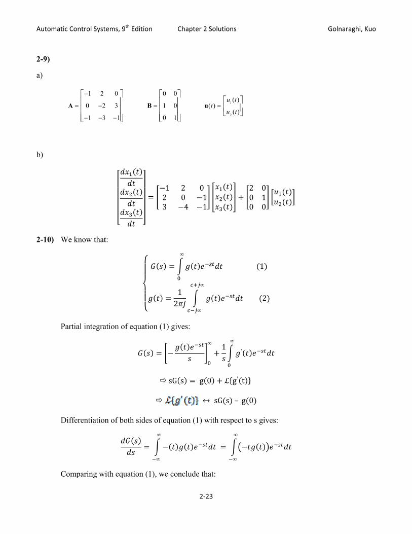
2-9)
a)
1
2
1 2 0 0 0( )
0 2 3 1 0 ( )( )
1 3 1 0 1
u tt
u t
−
= − = =
− − −
⎡ ⎤ ⎡ ⎤⎡ ⎤⎢ ⎥ ⎢ ⎥⎢ ⎥⎢ ⎥ ⎢ ⎥ ⎣ ⎦⎢ ⎥ ⎢ ⎥⎣ ⎦ ⎣ ⎦
A B u
1 2 02 0 13 4 1
2 00 10 0
b)
2-10) We know that:
∞
1
12
∞
∞
2
Partial integration of equation (1) gives:
∞ 1 ′
∞
sG s g 0 g′ t
sG s – g 0
Differentiation of both sides of equation (1) with respect to s gives:
∞
∞
∞
∞
Comparing with equation (1), we conclude that:
2‐23

Automatic Control Systems, 9th Edition Chapter 2 Solutions Golnaraghi, Kuo
2-11) Let g(t) = ∞ then
Using Laplace transform and differentiation property, we have X(s) = sG(s)
Therefore G(s) = , which means:
∞
∞
1
2-12) By Laplace transform definition:
∞
Now, consider τ = t - T, then:
∞ ∞
Which means: ↔
2-13) Consider:
f(t) = g1(t) g2(t) =
By Laplace transform definition:
By using time shifting theorem, we have:
2‐24

Automatic Control Systems, 9th Edition Chapter 2 Solutions Golnaraghi, Kuo
·
Let’s consider g(t) = g1(t) g2(t)
By inverse Laplace Transform definition, w ve e ha
12
Then
Where
therefore:
12 G s G s
2-14) a) We know that
= = sG(s) + g(0)
When s ∞ , it can be written as:
2‐25

Automatic Control Systems, 9th Edition Chapter 2 Solutions Golnaraghi, Kuo
0
As
0
Therefore: 0
b) By Laplace transform d ntiation property: iffere
0
As
∞ 0
Therefore
0 ∞ 0
which means:
∞
2‐15)
MATLAB code:
clear all;
syms t
s=tf('s')
f1 = (sin(2*t))^2
L1=laplace(f1)
2‐26
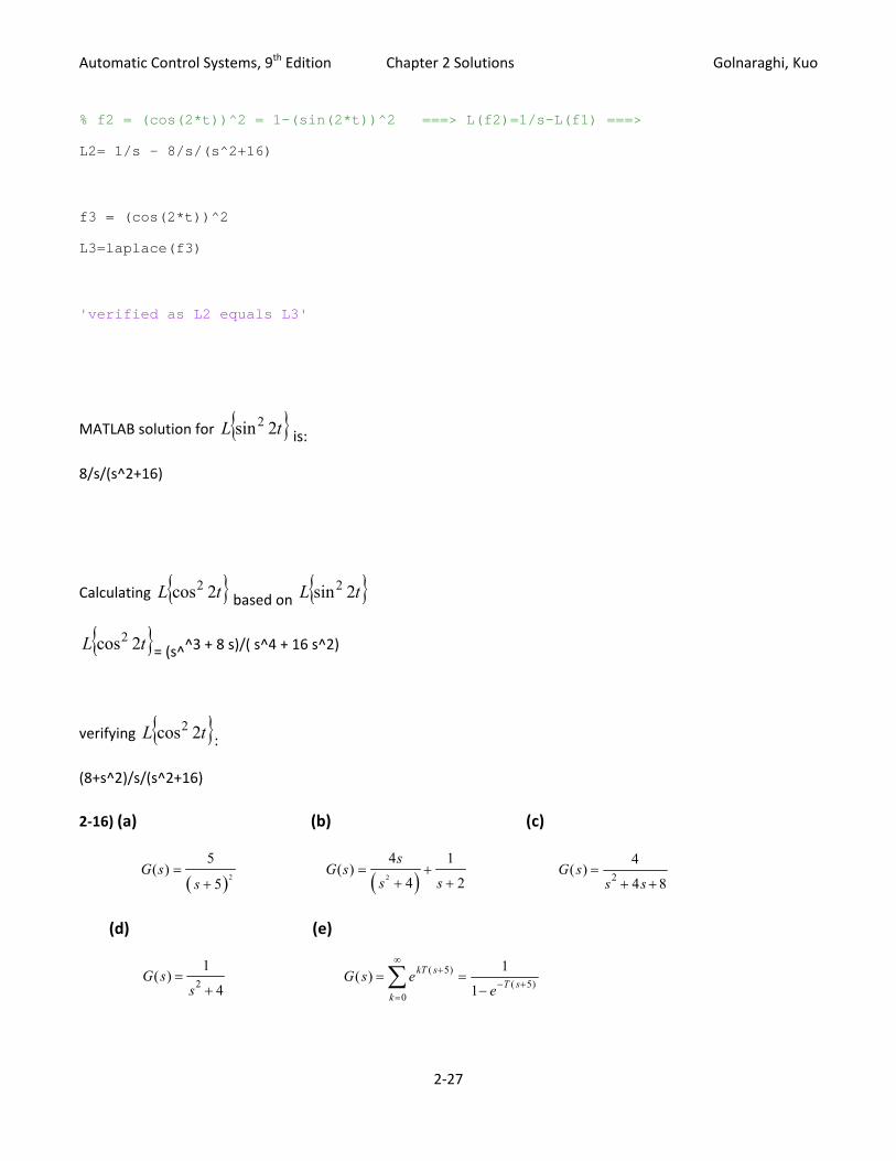
Automatic Control Systems, 9th Edition Chapter 2 Solutions Golnaraghi, Kuo % f2 = (cos(2*t))^2 = 1-(sin(2*t))^2 ===> L(f2)=1/s-L(f1) ===>
L2= 1/s - 8/s/(s^2+16)
f3 = (cos(2*t))^2
L3=laplace(f3)
'verified as L2 equals L3'
{ }tL 2sin2 is: MATLAB solution for
8/s/(s^2+16)
{ } { }tL 2cos2 based on tL 2sin2 Calculating
{ }tL 2cos2= (s^^3 + 8 s)/( s^4 + 16 s^2)
{ }t2cos2L : verifying
(8+s^2)/s/(s^2+16)
2‐16) (a)
( )
(b) (c)
2
5( )
5s=
+ ( )G s
2
4 1( )
4 2
sG s
s s= + G s
+ + s s( ) =
+ +
4
4 82
(d) (e)
G ss
( ) =+
1
42 G s ekT s
k
( ) ( )= =+
e T s( )−=
∞
− +5
1
1∑ 5
0
2‐27

Automatic Control Systems, 9th Edition Chapter 2 Solutions Golnaraghi, Kuo
)(5)( 5 tutetg st−=
g t t t e u tt
2‐17) Note: %section (e) requires assignment of T and a numerical loop calculation
MATLAB code:
clear all;
syms t u
f1 = 5*t*exp(-5*t)
L1=laplace(f1)
f2 = t*sin(2*t)+exp(-2*t)
L2=laplace(f2)
f3 = 2*exp(-2*t)*sin(2*t)
L3=laplace(f3)
f4 = sin(2*t)*cos(2*t)
L4=laplace(f4)
%section (e) requires assignment of T and a numerical loop calculation
(a)
Answer: 5/(s+5)^2
(b) s( ) ( sin ) ( )= + −2 2
t
Answer: 4*s/(s^2+4)^2+1/(s+2)
(c) g t e t uts( ) sin (= −2 22 )
Answer: 4/(s^2+4*s+8)
2‐28
Automatic Control Systems, 9th Edition Chapter 2 Solutions Golnaraghi, Kuo (d) g t t t u ts( ) sin cos ( )= 2 2
Answer: 2/(s^2+16)
(e) g t e t kTkT
k
( ) ( )= −
=
∞
∑ 5
0
δ − where δ(t) = unit‐impulse function
%section (e) requires assignment of T and a numerical loop calculation
2‐18 (a)
( ) ( )
( ) ( )
2 3
22
1 1( ) 1 2 2 2
1
( ) ( ) 2 ( 1) ( 2) 0 2
1 1( ) 1 2 1
s s s ss
s s s
( ) ( ) 2 ( 1) 2 ( 2) 2 ( 3)
s
T s s s
s s sT
eG s e e e
s s
g t u t u t u t t
G s e e es s
−− − −
−
− − −
−= − + − + =
+
= − − + − ≤ ≤
= − + = −
L
g t u t u t u t u t
e
= − − + − − − +L
g t g t k u t k G s e ee
T ss ks
s
s( ) ( ) ( ) ( ) ( )= − − = − =−− −
s s ekk ( )+
−
−=
∞
= 100
∞
∑∑ 2 21
112 2
( ) 2 ( ) 4( 0.5) ( 0.5) 4( 1) ( 1) 4( 1.5) ( 1.5)s s s sg t tu t t u t t u t t u t= − − − + − − − − − +L
(b)
( ) ( )( )
0.52 12s
0.5 1.52 2 0.5( ) 1 2 2 2
1s s s
s
e−−
t
G s e e es s e
− − −−= − + − + =
+L
g t tu t t u t t u tT s s s( ) ( ) ( . ( . ) ( )= − − − + − − ≤ ≤2 4 0 5) 0 5) 2( 1 1 0 1
( ) ( )20.5 0.52 2
2 2( ) 1 2 1s s s
TG s e e e− − −= − + = − s s
( )( )( )
0.5
2 2 0.50 0
2 1( ) ( ) ( ) ( ) 1
1
20.52s
s ksT s s
k k
eg t g t k u t k G s e e
s s e
−
−= =
−= − − = − =
+∑ ∑
s (
∞ ∞− −
2‐19)
g t t u t t u t u t t u t t u t u ts s s s s( ) ( ) ( ) ( ) ( ) ( ) ( ) ( ) ( (= + − − − − − − − − + − − + − 3)1 1 1 2 1 2 2 3) 3)
2‐29
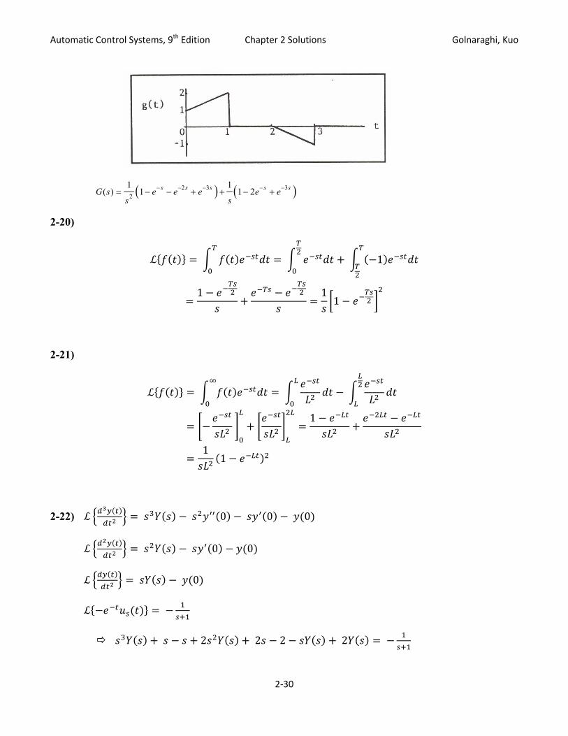
Automatic Control Systems, 9th Edition Chapter 2 Solutions Golnaraghi, Kuo
( ) ( )2 3 32
1 1( ) 1 1 2s s s s sG s e e e e e
s s− − − − −= − − + + − +
2-20)
1
1 11
2-21)
1
11
2-22) 0 0 0
0 0
0
2 2 2 2
2‐30

Automatic Control Systems, 9th Edition Chapter 2 Solutions Golnaraghi, Kuo
2 2 2 2
2‐23
MATLAB code:
clear all;
syms t u s x1 x2 Fs
f1 = exp(-2*t)
L1=laplace(f1)/(s^2+5*s+4);
Eq2=solve('s*x1=1+x2','s*x2=-2*x1-3*x2+1','x1','x2')
f2_x1=Eq2.x1
f2_x2=Eq2.x2
f3=solve('(s^3-s+2*s^2+s+2)*Fs=-1+2-(1/(1+s))','Fs')
Here is the solution provided by MATLAB:
Part (a): F(s)=1/(s+2)/(s^2+5*s+4)
Part (b): X1(s)= (4+s)/(2+3*s+s^2)
X2(s)= (s‐2)/(2+3*s+s^2)
Part (c): F(s) = s/(1+s)/(s^3+2*s^2+2)
2‐31

Automatic Control Systems, 9th Edition Chapter 2 Solutions Golnaraghi, Kuo 2‐24)
MATLAB code:
clear all;
syms s Fs
f3=solve('s^2*Fs-Fs=1/(s-1)','Fs')
Answer from MATLAB: Y(s)= 1/(s-1)/(s^2-1)
2‐25)
MATLAB code:
clear all;
syms s CA1 CA2 CA3
v1=1000;
v2=1500;
v3=100;
k1=0.1
k2=0.2
k3=0.4
f1='s*CA1=1/v1*(1000+100*CA2-1100*CA1-k1*v1*CA1)'
f2='s*CA2=1/v2*(1100*CA1-1100*CA2-k2*v2*CA2)'
f3='s*CA3=1/v3*(1000*CA2-1000*CA3-k3*v3*CA3)'
Sol=solve(f1,f2,f3,'CA1','CA2','CA3')
CA1=Sol.CA1
CA3=Sol.CA2
CA4=Sol.CA3
2‐32

Automatic Control Systems, 9th Edition Chapter 2 Solutions Golnaraghi, Kuo Solution from MATLAB:
CA1(s) = 1000*(s*v2+1100+k2*v2)/(1100000+s^2*v1*v2+1100*s*v1+s*v1*k2*v2+1100*s*v2+1100*k2*v2+k1*v1*s*v2+1100*k1*v1+k1*v1*k2*v2)
CA3(s) =
1100000/(1100000+s^2*v1*v2+1100*s*v1+s*v1*k2*v2+1100*s*v2+1100*k2*v2+k1*v1*s*v2+1100*k1*v1+k1*v1*k2*v2)
CA4 (s)=
1100000000/(1100000000+1100000*s*v3+1000*s*v1*k2*v2+1100000*s*v1+1000*k1*v1*s*v2+1000*k1*v1*k2*v2+1100*s*v1*k3*v3+1100*s*v2*k3*v3+1100*k2*v2*s*v3+1100*k2*v2*k3*v3+1100*k1*v1*s*v3+1100*k1*v1*k3*v3+1100000*k1*v1+1000*s^2*v1*v2+1100000*s*v2+1100000*k2*v2+1100000*k3*v3+s^3*v1*v2*v3+1100*s^2*v1*v3+1100*s^2*v2*v3+s^2*v1*v2*k3*v3+s^2*v1*k2*v2*v3+s*v1*k2*v2*k3*v3+k1*v1*s^2*v2*v3+k1*v1*s*v2*k3*v3+k1*v1*k2*v2*s*v3+k1*v1*k2*v2*k3*v3)
2-26) (a)
G ss s s
g t e e tt t( )) (
( )= −+
++
= − + ≥− −1
3
1
2( 2
1
3 3)
1
3
1
2
1
302 3
(b)
G ss s s
g t e te et t t( ).
( )
.( ) . .=
−
++
++
+= − + +− − −2 5
1
5
1
2 5
32 5 5 2 52
3 t ≥ 0
(c)
( ) [ ]( 1)50 20 30 202( 1) ( 1)s t
ss
t u t− − −+− −2( ) ( ) 50 20 30 cos 2( 1) 5 sin
1 4G s e g t e t
s s s= − − = − − − −
+ +
(d)
s s G s
s s s s s s( ) = −
−
+ += +
+ +−
s s+ +
1 1
2
1 1
2 22 2 2 Taking the inverse Laplace transform,
( )[ ] ( )0.5 o 0.5( ) 1 1.069 sin1.323 sin 1.323 69.3 1 1.447 sin1.323 cos1.323 0t tg t e t t e t t t− −= + + − = + − ≥
(e) g t t e tt( ) .= ≥−0 5 02
(f)Try using MATLAB
>> b=num*2
2‐33

Automatic Control Systems, 9th Edition Chapter 2 Solutions Golnaraghi, Kuo
b =
2 2 2
>>num =
1 1 1
>> denom1=[1 1]
denom1 =
1 1
>> denom2=[1 5 5]
denom2 =
1 5 5
>> num*2
ans =
2 2 2
>> denom=conv([1 0],conv(denom1,denom2))
denom =
1 6 10 5 0
>> b=num*2
b =
2 2 2
>> a=denom
a =
1 6 10 5 0
>> [r, p, k] = residue(b,a)
r =
-0.9889
2‐34

Automatic Control Systems, 9th Edition Chapter 2 Solutions Golnaraghi, Kuo
2.5889
-2.0000
0.4000
p =
-3.6180
-1.3820
-1.0000
0
k = [ ]
If there are no multiple roots, then
The number of poles n is
1 2
1 2
... n
n
rr rb ka s p s p s p= + + + +
+ + +
In this case, p1 and k are zero. Hence,
3.618 2.5889
0.4 0.9889 2.5889 2( )3.6180 1.3820 1
( )g t =
(g)
0.4 0.9889 1.3820 2t t t
G ss s s s
e e e− − −
= − + −+ + +
− + −
G s 2e 2e 2e 1
(h)
3
2‐35

Automatic Control Systems, 9th Edition Chapter 2 Solutions Golnaraghi, Kuo
(i)
2‐27
MATLAB code:
clear all;
syms s
f1=1/(s*(s+2)*(s+3))
F1=ilaplace(f1)
f2=10/((s+1)^2*(s+3))
F2=ilaplace(f2)
f3=10*(s+2)/(s*(s^2+4)*(s+1))*exp(-s)
F3=ilaplace(f3)
f4=2*(s+1)/(s*(s^2+s+2))
F4=ilaplace(f4)
f5=1/(s+1)^3
F5=ilaplace(f5)
f6=2*(s^2+s+1)/(s*(s+1.5)*(s^2+5*s+5))
F6=ilaplace(f6)
s=tf('s')
f7=(2+2*s*pade(exp(-1*s),1)+4*pade(exp(-2*s),1))/(s^2+3*s+2) %using Pade command for exponential term
2‐36
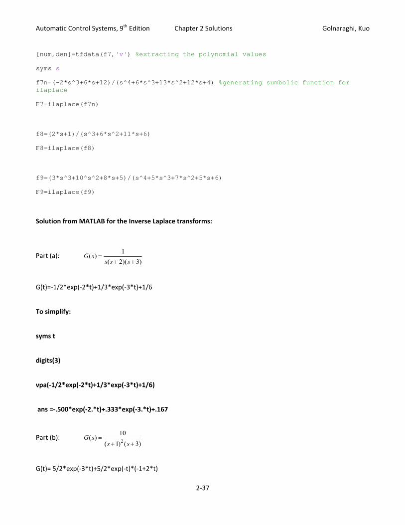
Automatic Control Systems, 9th Edition Chapter 2 Solutions Golnaraghi, Kuo [num,den]=tfdata(f7,'v') %extracting the polynomial values
syms s
f7n=(-2*s^3+6*s+12)/(s^4+6*s^3+13*s^2+12*s+4) %generating sumbolic function for ilaplace
F7=ilaplace(f7n)
f8=(2*s+1)/(s^3+6*s^2+11*s+6)
F8=ilaplace(f8)
f9=(3*s^3+10^s^2+8*s+5)/(s^4+5*s^3+7*s^2+5*s+6)
F9=ilaplace(f9)
Solution from MATLAB for the Inverse Laplace transforms:
Part (a): G ss s s
( )( )( )
=+ +
12 3
G(t)=‐1/2*exp(‐2*t)+1/3*exp(‐3*t)+1/6
To simplify:
syms t
digits(3)
vpa(‐1/2*exp(‐2*t)+1/3*exp(‐3*t)+1/6)
ans =‐.500*exp(‐2.*t)+.333*exp(‐3.*t)+.167
Part (b): G ss s
( )( ) ( )
=+ +
101 32
G(t)= 5/2*exp(‐3*t)+5/2*exp(‐t)*(‐1+2*t)
2‐37
Automatic Control Systems, 9th Edition Chapter 2 Solutions Golnaraghi, Kuo
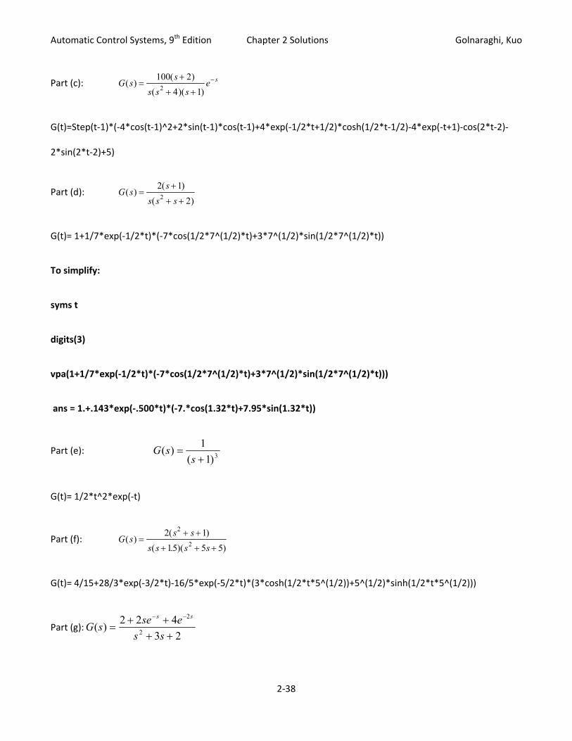
Part (c): G ss
s s se s( )
( )( )( )
=+
+ +−100 2
4 12
G(t)=Step(t‐1)*(‐4*cos(t‐1)^2+2*sin(t‐1)*cos(t‐1)+4*exp(‐1/2*t+1/2)*cosh(1/2*t‐1/2)‐4*exp(‐t+1)‐cos(2*t‐2)‐
2*sin(2*t‐2)+5)
Part (d): G ss
s s s( )
( )( )
=+
+ +
2 122
G(t)= 1+1/7*exp(‐1/2*t)*(‐7*cos(1/2*7^(1/2)*t)+3*7^(1/2)*sin(1/2*7^(1/2)*t))
To simplify:
syms t
digits(3)
vpa(1+1/7*exp(‐1/2*t)*(‐7*cos(1/2*7^(1/2)*t)+3*7^(1/2)*sin(1/2*7^(1/2)*t)))
ans = 1.+.143*exp(‐.500*t)*(‐7.*cos(1.32*t)+7.95*sin(1.32*t))
Part (e): 3)1(1)(+
=s
sG
G(t)= 1/2*t^2*exp(‐t)
Part (f): G ss s
s s s s( )
( )( . )( )
=+ +
+ + +
2 115 5 5
2
2
G(t)= 4/15+28/3*exp(‐3/2*t)‐16/5*exp(‐5/2*t)*(3*cosh(1/2*t*5^(1/2))+5^(1/2)*sinh(1/2*t*5^(1/2)))
Part (g): 23
422)( 2
2
++++
=−−
ssesesG
ss
2‐38

Automatic Control Systems, 9th Edition Chapter 2 Solutions Golnaraghi, Kuo G(t)= 2*exp(‐2*t)*(7+8*t)+8*exp(‐t)*(‐2+t)
Part (h): 6116
12)( 23 ++++
=sss
ssG
G(t)= ‐1/2*exp(‐t)+3*exp(‐2*t)‐5/2*exp(‐3*t)
Part (i): 6575
58103)( 234
23
+++++++
=ssss
ssssG
G(t)= ‐7*exp(‐2*t)+10*exp(‐3*t)‐
1/10*ilaplace(10^(2*s)/(s^2+1)*s,s,t)+1/10*ilaplace(10^(2*s)/(s^2+1),s,t)+1/10*sin(t)*(10+dirac(t)*(‐exp(‐
3*t)+2*exp(‐2*t)))
2‐39
Automatic Control Systems, 9th Edition Chapter 2 Solutions Golnaraghi, Kuo
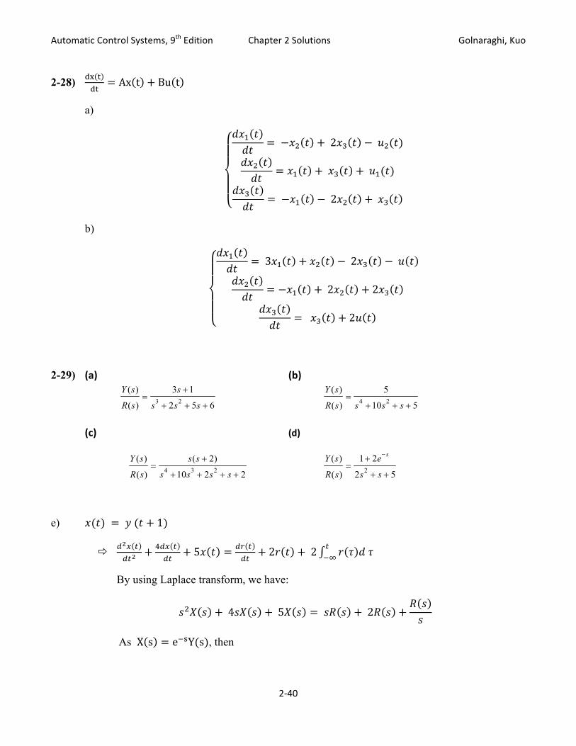
2-28) Ax t Bu t
2
2
a)
3 2
2 2
2
b)
2-29) (a) (b)
3 2
( ) 3 1
( ) 2 5 6
Y s s
R s s s s
+=
+ + + 4 2
( ) 5
( ) 10 5
Y s
R s s s s=
+ + +
(c) (d)
4 3 2( ) 10 2 2R s s s s s=
+ + + +
( ) ( 2)Y s s s + 2( ) 2 5
s( ) 1 2Y s e−+
R s s s=
+ +
e) 1
5 2 2
By using Laplace transform, we have:
4 5 2
As X s e Y s , then
2‐40
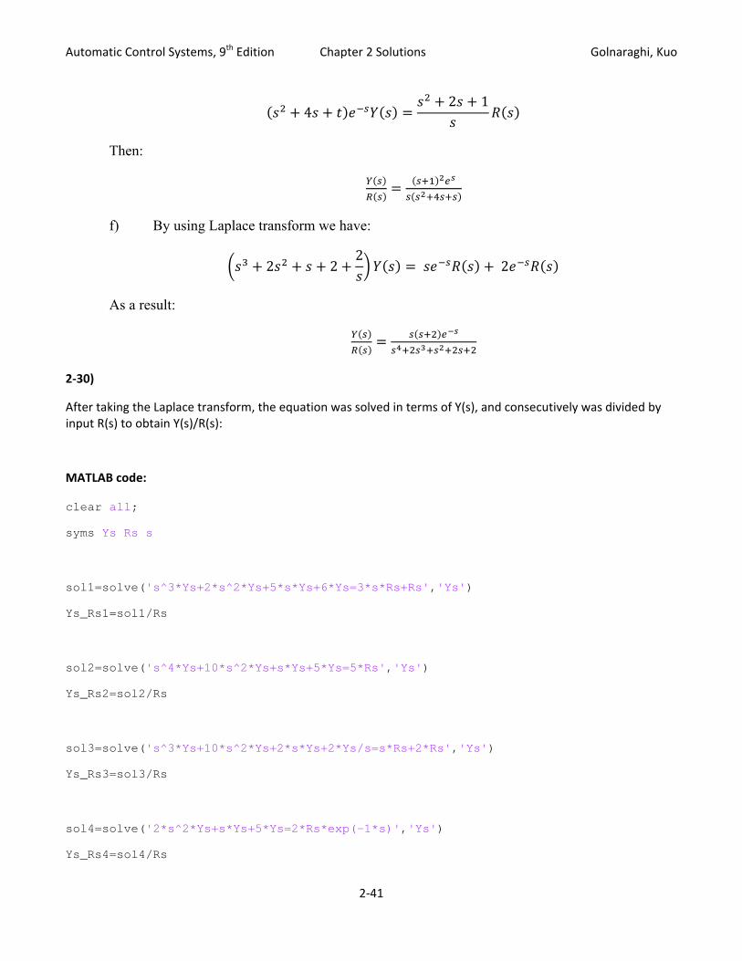
Automatic Control Systems, 9th Edition Chapter 2 Solutions Golnaraghi, Kuo
42 1
Then:
f) By using Laplace transform we have:
2 22
2
As a result:
2‐30)
After taking the Laplace transform, the equation was solved in terms of Y(s), and consecutively was divided by input R(s) to obtain Y(s)/R(s):
MATLAB code:
clear all;
syms Ys Rs s
sol1=solve('s^3*Ys+2*s^2*Ys+5*s*Ys+6*Ys=3*s*Rs+Rs','Ys')
Ys_Rs1=sol1/Rs
sol2=solve('s^4*Ys+10*s^2*Ys+s*Ys+5*Ys=5*Rs','Ys')
Ys_Rs2=sol2/Rs
sol3=solve('s^3*Ys+10*s^2*Ys+2*s*Ys+2*Ys/s=s*Rs+2*Rs','Ys')
Ys_Rs3=sol3/Rs
sol4=solve('2*s^2*Ys+s*Ys+5*Ys=2*Rs*exp(-1*s)','Ys')
Ys_Rs4=sol4/Rs
2‐41

Automatic Control Systems, 9th Edition Chapter 2 Solutions Golnaraghi, Kuo %Note: Parts E&F are too complicated with MATLAB, Laplace of integral is not executable in MATLAB.....skipped
MATLAB Answers:
Part (a): Y(s)/R(s)= (3*s+1)/(5*s+6+s^3+2*s^2);
Part (b): Y(s)/R(s)= 5/(10*s^2+s+5+s^4)
Part (c): Y(s)/R(s)= (s+2)*s/(2*s^2+2+s^4+10*s^3)
Part (d): Y(s)/R(s)= 2*exp(‐s)/(2*s^2+s+5)
%Note: Parts E&F are too complicated with MATLAB, Laplace of integral is not executable in MATLAB.....skipped
2‐31
MATLAB code:
clear all;
s=tf('s')
%Part a
Eq=10*(s+1)/(s^2*(s+4)*(s+6));
[num,den]=tfdata(Eq,'v');
[r,p] = residue(num,den)
%Part b
Eq=(s+1)/(s*(s+2)*(s^2+2*s+2));
[num,den]=tfdata(Eq,'v');
[r,p] = residue(num,den)
%Part c
Eq=5*(s+2)/(s^2*(s+1)*(s+5));
[num,den]=tfdata(Eq,'v');
2‐42

Automatic Control Systems, 9th Edition Chapter 2 Solutions Golnaraghi, Kuo [r,p] = residue(num,den)
%Part d
Eq=5*(pade(exp(-2*s),1))/(s^2+s+1); %Pade approximation oreder 1 used
[num,den]=tfdata(Eq,'v');
[r,p] = residue(num,den)
%Part e
Eq=100*(s^2+s+3)/(s*(s^2+5*s+3));
[num,den]=tfdata(Eq,'v');
[r,p] = residue(num,den)
%Part f
Eq=1/(s*(s^2+1)*(s+0.5)^2);
[num,den]=tfdata(Eq,'v');
[r,p] = residue(num,den)
%Part g
Eq=(2*s^3+s^2+8*s+6)/((s^2+4)*(s^2+2*s+2));
[num,den]=tfdata(Eq,'v');
[r,p] = residue(num,den)
%Part h
Eq=(2*s^4+9*s^3+15*s^2+s+2)/(s^2*(s+2)*(s+1)^2);
[num,den]=tfdata(Eq,'v');
[r,p] = residue(num,den)
The solutions are presented in the form of two vectors, r and p, where for each case, the partial fraction expansion is equal to:
2‐43

Automatic Control Systems, 9th Edition Chapter 2 Solutions Golnaraghi, Kuo
2‐44
n
nps
rps
rps
rsasb
−++
−+
−= ...
)()(
2
2
1
1
Following are r and p vectors for each part:
Part(a):
r =0.6944
‐0.9375
0.2431
0.4167
p =‐6.0000
‐4.0000
0
0
Part(b):
r =0.2500
‐0.2500 ‐ 0.0000i
‐0.2500 + 0.0000i
0.2500
p =‐2.0000
‐1.0000 + 1.0000i
Automatic Control Systems, 9th Edition Chapter 2 Solutions Golnaraghi, Kuo
‐1.0000 ‐ 1.0000i
0
Part(c):
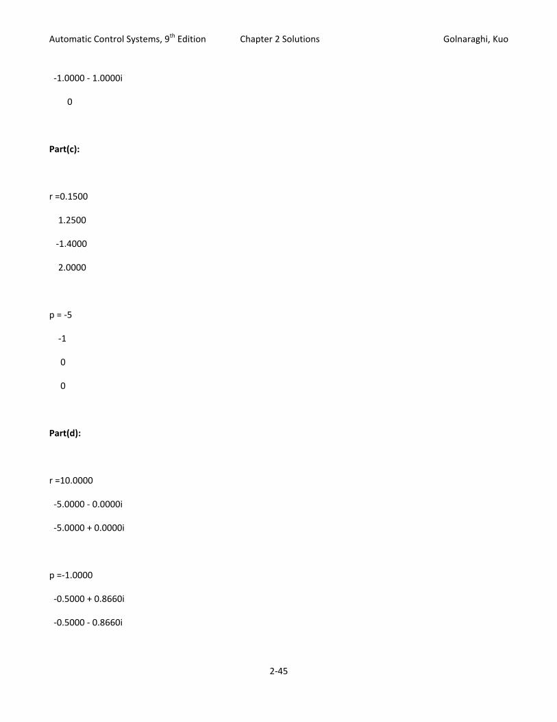
r =0.1500
1.2500
‐1.4000
2.0000
p = ‐5
‐1
0
0
Part(d):
r =10.0000
‐5.0000 ‐ 0.0000i
‐5.0000 + 0.0000i
p =‐1.0000
‐0.5000 + 0.8660i
‐0.5000 ‐ 0.8660i
2‐45
Automatic Control Systems, 9th Edition Chapter 2 Solutions Golnaraghi, Kuo
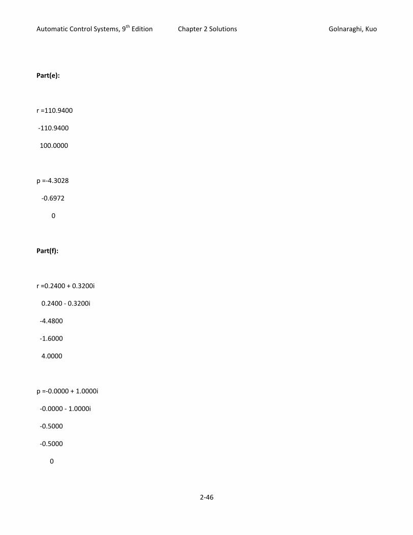
Part(e):
r =110.9400
‐110.9400
100.0000
p =‐4.3028
‐0.6972
0
Part(f):
r =0.2400 + 0.3200i
0.2400 ‐ 0.3200i
‐4.4800
‐1.6000
4.0000
p =‐0.0000 + 1.0000i
‐0.0000 ‐ 1.0000i
‐0.5000
‐0.5000
0
2‐46
Automatic Control Systems, 9th Edition Chapter 2 Solutions Golnaraghi, Kuo
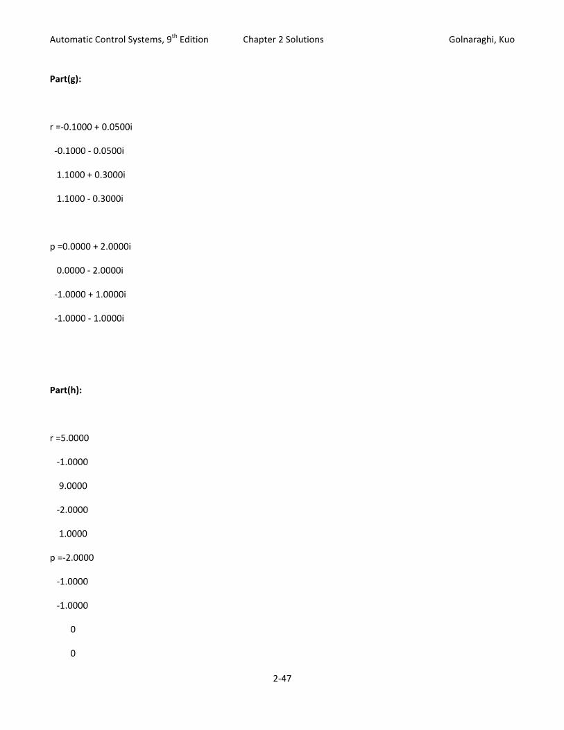
Part(g):
r =‐0.1000 + 0.0500i
‐0.1000 ‐ 0.0500i
1.1000 + 0.3000i
1.1000 ‐ 0.3000i
p =0.0000 + 2.0000i
0.0000 ‐ 2.0000i
‐1.0000 + 1.0000i
‐1.0000 ‐ 1.0000i
Part(h):
r =5.0000
‐1.0000
9.0000
‐2.0000
1.0000
p =‐2.0000
‐1.0000
‐1.0000
0
0
2‐47
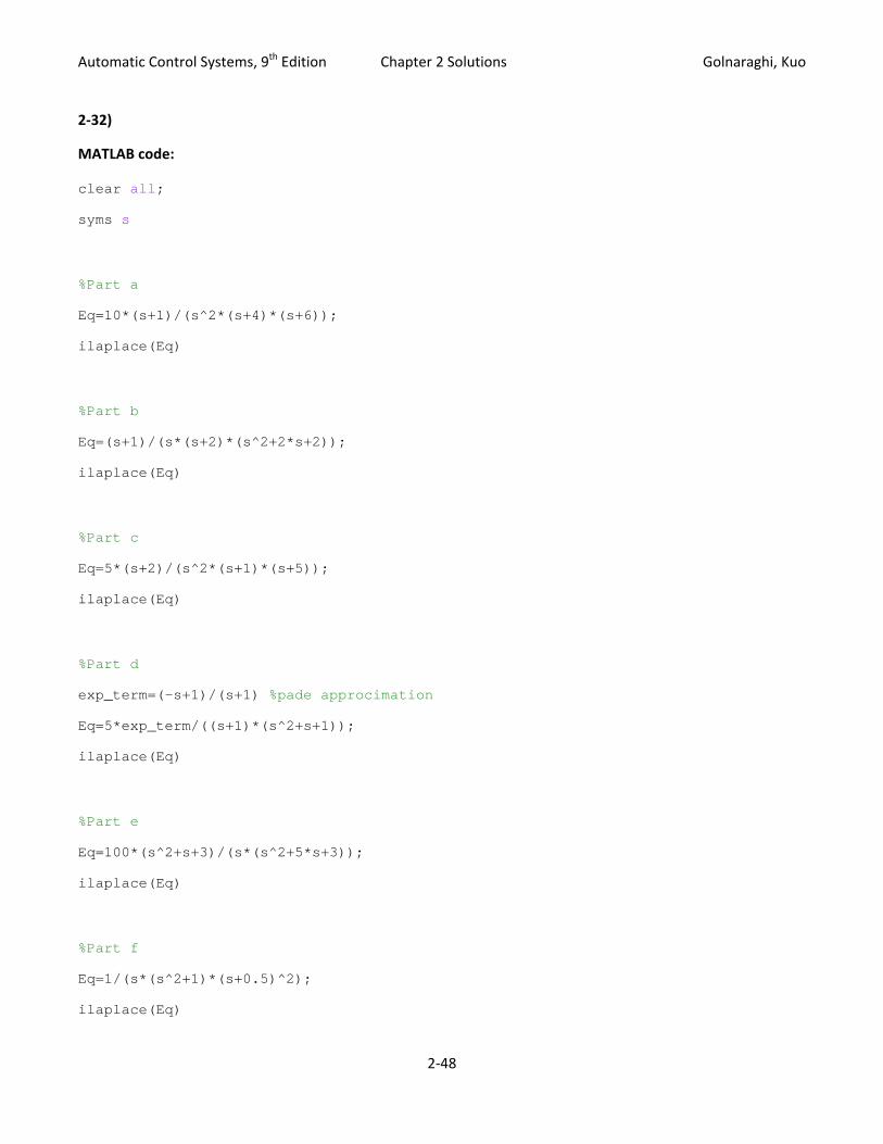
Automatic Control Systems, 9th Edition Chapter 2 Solutions Golnaraghi, Kuo 2‐32)
MATLAB code:
clear all;
syms s
%Part a
Eq=10*(s+1)/(s^2*(s+4)*(s+6));
ilaplace(Eq)
%Part b
Eq=(s+1)/(s*(s+2)*(s^2+2*s+2));
ilaplace(Eq)
%Part c
Eq=5*(s+2)/(s^2*(s+1)*(s+5));
ilaplace(Eq)
%Part d
exp_term=(-s+1)/(s+1) %pade approcimation
Eq=5*exp_term/((s+1)*(s^2+s+1));
ilaplace(Eq)
%Part e
Eq=100*(s^2+s+3)/(s*(s^2+5*s+3));
ilaplace(Eq)
%Part f
Eq=1/(s*(s^2+1)*(s+0.5)^2);
ilaplace(Eq)
2‐48

Automatic Control Systems, 9th Edition Chapter 2 Solutions Golnaraghi, Kuo
%Part g
Eq=(2*s^3+s^2+8*s+6)/((s^2+4)*(s^2+2*s+2));
ilaplace(Eq)
%Part h
Eq=(2*s^4+9*s^3+15*s^2+s+2)/(s^2*(s+2)*(s+1)^2);
ilaplace(Eq)
MATLAB Answers:
Part(a):
G(t)= ‐15/16*exp(‐4*t)+25/36*exp(‐6*t)+35/144+5/12*t
To simplify:
syms t
digits(3)
vpa(‐15/16*exp(‐4*t)+25/36*exp(‐6*t)+35/144+5/12*t)
ans =‐.938*exp(‐4.*t)+.694*exp(‐6.*t)+.243+.417*tPart(b):
G(t)= 1/4*exp(‐2*t)+1/4‐1/2*exp(‐t)*cos(t)
Part(c):
G(t)= 5/4*exp(‐t)‐7/5+3/20*exp(‐5*t)+2*t
2‐49

Automatic Control Systems, 9th Edition Chapter 2 Solutions Golnaraghi, Kuo
Part(d):
G(t)= ‐5*exp(‐1/2*t)*(cos(1/2*3^(1/2)*t)+3^(1/2)*sin(1/2*3^(1/2)*t))+5*(1+2*t)*exp(‐t)
Part(e):
G(t)= 100‐800/13*exp(‐5/2*t)*13^(1/2)*sinh(1/2*t*13^(1/2))
Part(f):
G(t)= 4+12/25*cos(t)‐16/25*sin(t)‐8/25*exp(‐1/2*t)*(5*t+14)
Part(g):
G(t)= ‐1/5*cos(2*t)‐1/10*sin(2*t)+1/5*(11*cos(t)‐3*sin(t))*exp(‐t)
Part(h):
G(t)= ‐2+t+5*exp(‐2*t)+(‐1+9*t)*exp(‐t)
2‐50
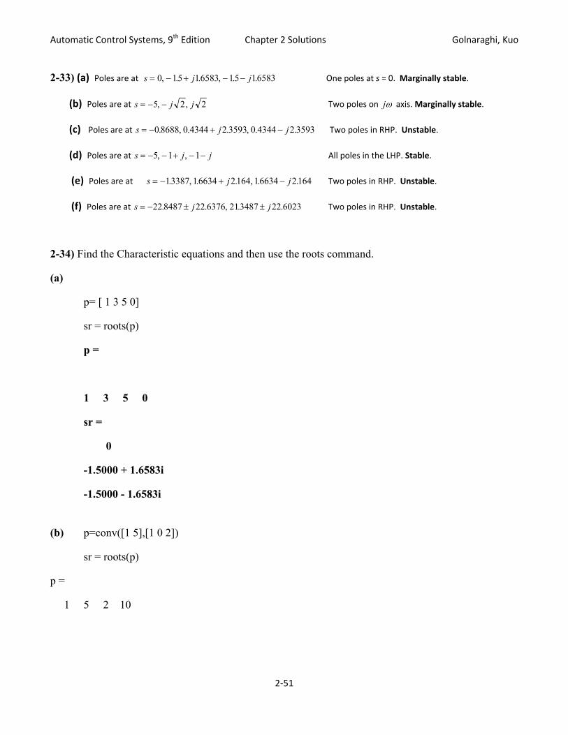
Automatic Control Systems, 9th Edition Chapter 2 Solutions Golnaraghi, Kuo 2-33) (a) Poles are at s j j= − + − −0 15 16583 15 16583, . . , . . One poles at s = 0. Marginally stable.
(b) Poles are at s j j= − −5 2, , 2 Two poles on jω axis. Marginally stable.
(c) Poles are at s j= − + j−0 8688 0 2 3593 0 2 3593. , .4344 . , .4344 . Two poles in RHP. Unstable.
(d) Poles are at s j j= − − + − −5 1 1, , All poles in the LHP. Stable.
(e) Poles are at s j= − + j−13387 16634 2164, 16634 2164. , . . . . Two poles in RHP. Unstable.
(f) Poles are at s j= − ± j±22 8487 22 6376 213487 22 6023. . , . . Two poles in RHP. Unstable.
2-34) Find the Characteristic equations and then use the roots command.
(a)
p= [ 1 3 5 0]
sr = roots(p)
p =
1 3 5 0
sr =
0
-1.5000 + 1.6583i
-1.5000 - 1.6583i
(b) p=conv([1 5],[1 0 2])
sr = roots(p)
p =
1 5 2 10
2‐51

Automatic Control Systems, 9th Edition Chapter 2 Solutions Golnaraghi, Kuo sr =
-5.0000
0.0000 + 1.4142i
0.0000 - 1.4142i
(c)
>> roots([1 5 5])
ans =
-3.6180
-1.3820
(d) roots(conv([1 5],[1 2 2]))
ans =
-5.0000
-1.0000 + 1.0000i
-1.0000 - 1.0000i
(e) roots([1 -2 3 10])
ans =
1.6694 + 2.1640i
1.6694 - 2.1640i
-1.3387
2‐52

Automatic Control Systems, 9th Edition Chapter 2 Solutions Golnaraghi, Kuo (f) roots([1 3 50 1 10^6])
-22.8487 +22.6376i
-22.8487 -22.6376i
21.3487 +22.6023i
21.3487 -22.6023i
Alternatively
Problem 2‐34
MATLAB code:
% Question 2-34,
clear all;
s=tf('s')
%Part a
Eq=10*(s+2)/(s^3+3*s^2+5*s);
[num,den]=tfdata(Eq,'v');
roots(den)
%Part b
Eq=(s-1)/((s+5)*(s^2+2));
[num,den]=tfdata(Eq,'v');
roots(den)
%Part c
Eq=1/(s^3+5*s+5);
[num,den]=tfdata(Eq,'v');
roots(den)
2‐53
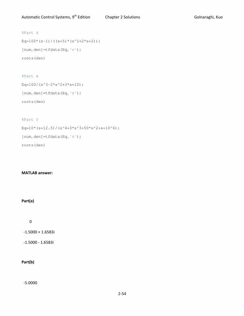
Automatic Control Systems, 9th Edition Chapter 2 Solutions Golnaraghi, Kuo %Part d
Eq=100*(s-1)/((s+5)*(s^2+2*s+2));
[num,den]=tfdata(Eq,'v');
roots(den)
%Part e
Eq=100/(s^3-2*s^2+3*s+10);
[num,den]=tfdata(Eq,'v');
roots(den)
%Part f
Eq=10*(s+12.5)/(s^4+3*s^3+50*s^2+s+10^6);
[num,den]=tfdata(Eq,'v');
roots(den)
MATLAB answer:
Part(a)
0
‐1.5000 + 1.6583i
‐1.5000 ‐ 1.6583i
Part(b)
‐5.0000
2‐54
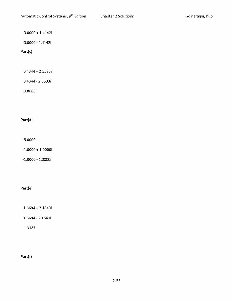
Automatic Control Systems, 9th Edition Chapter 2 Solutions Golnaraghi, Kuo
‐0.0000 + 1.4142i
‐0.0000 ‐ 1.4142i
Part(c)
0.4344 + 2.3593i
0.4344 ‐ 2.3593i
‐0.8688
Part(d)
‐5.0000
‐1.0000 + 1.0000i
‐1.0000 ‐ 1.0000i
Part(e)
1.6694 + 2.1640i
1.6694 ‐ 2.1640i
‐1.3387
Part(f)
2‐55

Automatic Control Systems, 9th Edition Chapter 2 Solutions Golnaraghi, Kuo
‐22.8487 +22.6376i
‐22.8487 ‐22.6376i
21.3487 +22.6023i
21.3487 ‐22.6023i
2-35)
(a) s s s3 225 10 450 0+ + + = Roots: − + −25 31 01537 4.214, 01537 4.214. , . .j
Routh Tabulation:
s
s
3
2
1 10
25 450
s
s
1
0
250 450
258 0
450
−= −
Two sign changes in the first column. Two roots in RHP.
(b) s s s3 225 10 50 0+ + + = Roots: − − + − −24.6769 01616 1 01616 1, . .4142, . .4142j j
Routh Tabulation:
s
s
3
2
1 10
25 50
s
s
1
0
250 50
258 0
50
−=
No sign changes in the first column. No roots in RHP.
(c) s s s3 225 250 10 0+ + + = Roots: − − + −0 0402 12 9 6566 9 6566. , .48 . , .j j
Routh Tabulation:
2‐56
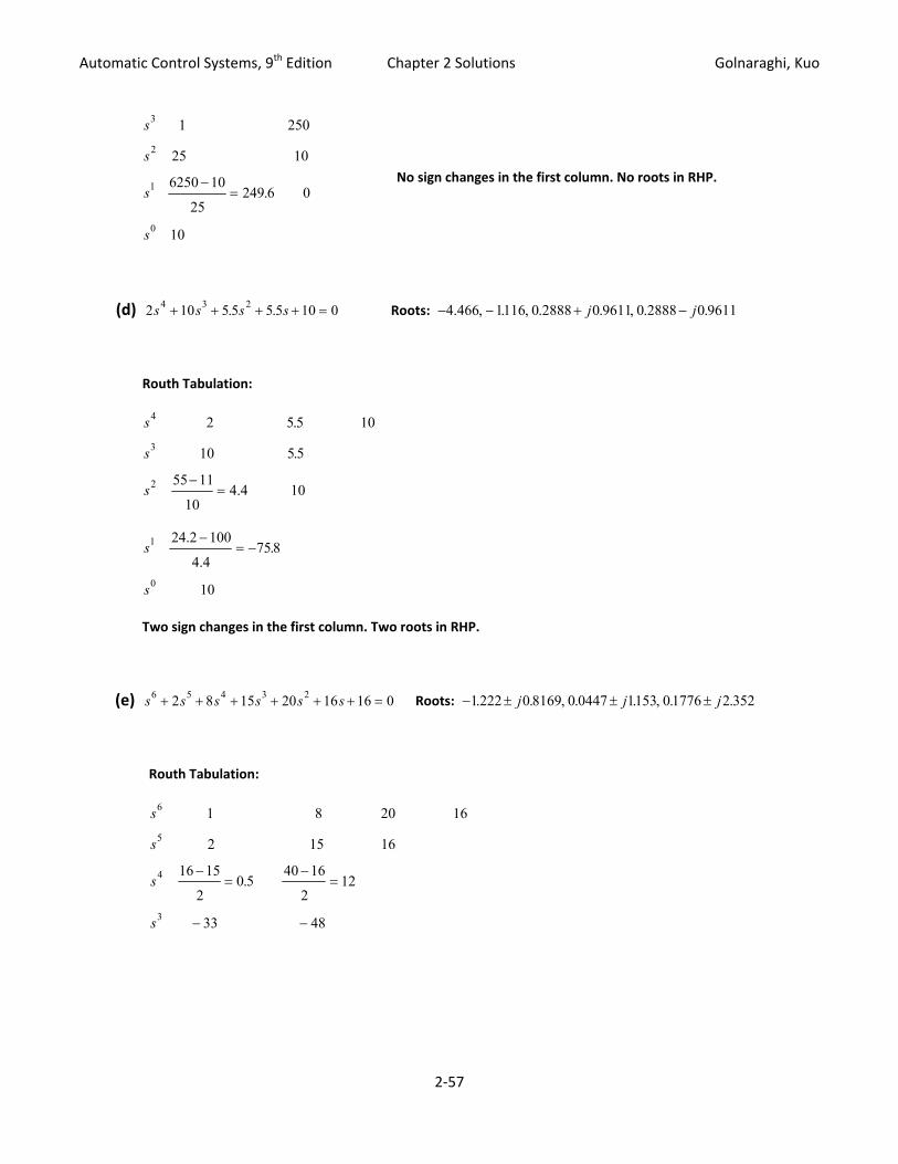
Automatic Control Systems, 9th Edition Chapter 2 Solutions Golnaraghi, Kuo
s
s
s
s
3
2
1
0
1 250
25 10
6250 10
25249 6 0
10
−= .
No sign changes in the first column. No roots in RHP.
(d) 2 10 5 5 5 5 104 3 2 0s s s s+ + + + =. . Roots: − − + −4.466 1116 0 0 9611 0 0 9611, . , .2888 . , .2888 .j j
Routh Tabulation:
s
s
s
4
3
2
2 5 5
10 5 5
55 11
104.4 10
.
.
−=
10
s
s
1
0
24.2 100
4.475 8
10
−= − .
Two sign changes in the first column. Two roots in RHP.
(e) s s s s s s6 5 4 3 22 8 15 20 16 16 0+ + + + + + = Roots: − ± ± ±1 0 8169 0 0447 1153 01776 2 352.222 . , . . , . .j j j
Routh Tabulation:
s
s
s
s
6
5
4
3
1 8 20 16
2 15 16
16 15
20 5
40 16
212
33 48
−=
−=
− −
.
2‐57
Automatic Control Systems, 9th Edition Chapter 2 Solutions Golnaraghi, Kuo
‐
s
s
s
2
1
0
396 24
3311 16
5411 528
11116 0
0
− +
−=
− += −
.27
.
.27.
Four sign changes in the first column. Four roots in RHP.
(f) s s s s4 3 22 10 20 5+ + + + = 0 Roots: − − + −0 1788 0 039 3105 0 039 3105.29, . , . . , . .j j
Routh Tabulation:
s
s
s
s
4
3
2
2
1 10 5
2 20
20 20
20 5
5
−=
ε ε Replace 0 in last row by
s
s
1
0
20 10 10
5
ε
ε ε
−≅ −
Two sign changes in first column. Two roots in RHP.
(g)
s8 1 8 20 16 0
s7 2 12 16 0 0
s6 2 12 16 0 0
s5 0 0 0 0 0
2 58
2 12 16
12 60 64

Automatic Control Systems, 9th Edition Chapter 2 Solutions Golnaraghi, Kuo
s5 12 60 64 0
s4 2 163 0 0
s3 28 64 0 0
s2 0.759 0 0 0
s1 28 0
s0 0
2-36) Use MATLAB roots command
a) roots([1 25 10 450])
ans =
-25.3075
0.1537 + 4.2140i
0.1537 - 4.2140i
b) roots([1 25 10 50])
ans =
-24.6769
-0.1616 + 1.4142i
-0.1616 - 1.4142i
c) roots([1 25 250 10])
ans =
-12.4799 + 9.6566i
-12.4799 - 9.6566i
2‐59

Automatic Control Systems, 9th Edition Chapter 2 Solutions Golnaraghi, Kuo
-0.0402
d) roots([2 10 5.5 5.5 10])
ans =
-4.4660
-1.1116
0.2888 + 0.9611i
0.2888 - 0.9611i
e) roots([1 2 8 15 20 16 16])
ans =
0.1776 + 2.3520i
0.1776 - 2.3520i
-1.2224 + 0.8169i
-1.2224 - 0.8169i
0.0447 + 1.1526i
0.0447 - 1.1526i
f) roots([1 2 10 20 5])
ans =
0.0390 + 3.1052i
0.0390 - 3.1052i
-1.7881
-0.2900
g) roots([1 2 8 12 20 16 16])
2‐60
Automatic Control Systems, 9th Edition Chapter 2 Solutions Golnaraghi, Kuo ans =
0.0000 + 2.0000i
0.0000 - 2.0000i
-1.0000 + 1.0000i
-1.0000 - 1.0000i
0.0000 + 1.4142i
0.0000 - 1.4142i
Alternatively use the approach in this Chapter’s Section 2‐14:
1. Activate MATLAB
2. Go to the directory containing the ACSYS software.
3. Type in
Acsys
4. Then press the “transfer function Symbolic button
2‐61

Automatic Control Systems, 9th Edition Chapter 2 Solutions Golnaraghi, Kuo
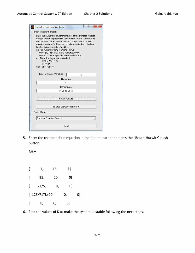
5. Enter the characteristic equation in the denominator and press the “Routh‐Hurwitz” push‐button.
RH =
[ 1, 10]
[ 25, 450]
[ -8, 0]
[ 450, 0]
Two sign changes in the first column. Two roots in RHP=> UNSTABLE
2-37) Use the MATLAB “roots” command same as in the previous problem.
2‐62

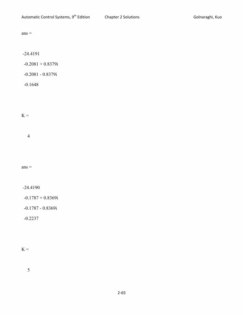
Automatic Control Systems, 9th Edition Chapter 2 Solutions Golnaraghi, Kuo 2-38) To solve using MATLAB, set the value of K in an iterative process and find the roots such that at least one root changes sign from negative to positive. Then increase resolution if desired.
Example: in this case 0<K<12 ( increase resolution by changing the loop to: for K=11:.1:12)
for K=0:12
K
roots([1 25 15 20 K])
end
K =
0
ans =
0
-24.4193
-0.2904 + 0.8572i
-0.2904 - 0.8572i
K =
1
ans =
2‐63
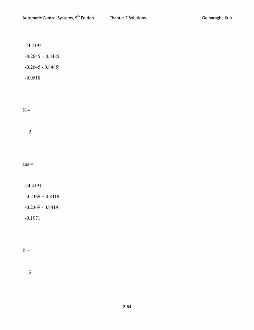
Automatic Control Systems, 9th Edition Chapter 2 Solutions Golnaraghi, Kuo
-24.4192
-0.2645 + 0.8485i
-0.2645 - 0.8485i
-0.0518
K =
2
ans =
-24.4191
-0.2369 + 0.8419i
-0.2369 - 0.8419i
-0.1071
K =
3
2‐64
Automatic Control Systems, 9th Edition Chapter 2 Solutions Golnaraghi, Kuo ans =
-24.4191
-0.2081 + 0.8379i
-0.2081 - 0.8379i
-0.1648
K =
4
ans =
-24.4190
-0.1787 + 0.8369i
-0.1787 - 0.8369i
-0.2237
K =
5
2‐65

Automatic Control Systems, 9th Edition Chapter 2 Solutions Golnaraghi, Kuo
ans =
-24.4189
-0.1496 + 0.8390i
-0.1496 - 0.8390i
-0.2819
K =
6
ans =
-24.4188
-0.1215 + 0.8438i
-0.1215 - 0.8438i
-0.3381
K =
7
2‐66

Automatic Control Systems, 9th Edition Chapter 2 Solutions Golnaraghi, Kuo
ans =
-24.4188
-0.0951 + 0.8508i
-0.0951 - 0.8508i
-0.3911
K =
8
ans =
-24.4187
-0.0704 + 0.8595i
-0.0704 - 0.8595i
-0.4406
K =
2‐67

Automatic Control Systems, 9th Edition Chapter 2 Solutions Golnaraghi, Kuo 9
ans =
-24.4186
-0.0475 + 0.8692i
-0.0475 - 0.8692i
-0.4864
K =
10
ans =
-24.4186
-0.0263 + 0.8796i
-0.0263 - 0.8796i
-0.5288
K =
2‐68

Automatic Control Systems, 9th Edition Chapter 2 Solutions Golnaraghi, Kuo
11
ans =
-24.4185
-0.0067 + 0.8905i
-0.0067 - 0.8905i
-0.5681
K =
12
ans =
-24.4184
0.0115 + 0.9015i
0.0115 - 0.9015i
-0.6046
Alternatively use the approach in this Chapter’s Section 2‐14:
2‐69

Automatic Control Systems, 9th Edition Chapter 2 Solutions Golnaraghi, Kuo
1. Activate MATLAB
2. Go to the directory containing the ACSYS software.
3. Type in
Acsys
4. Then press the “transfer function Symbolic button
2‐70
Automatic Control Systems, 9th Edition Chapter 2 Solutions Golnaraghi, Kuo
5. Enter the characteristic equation in the denominator and press the “Routh‐Hurwitz” push‐button.
RH =
[ 1, 15, k]
[ 25, 20, 0]
[ 71/5, k, 0]
[ ‐125/71*k+20, 0, 0]
[ k, 0, 0]
6. Find the values of K to make the system unstable following the next steps.
2‐71

Automatic Control Systems, 9th Edition Chapter 2 Solutions Golnaraghi, Kuo Alternative Problem 2‐36
Using ACSYS toolbar under “Transfer Function Symbolic”, the Routh‐Hurwitz option can be used to generate RH matrix based on denominator polynhomial. The system is stable if and only if the first column of this matrix contains NO negative values.
MATLAB code: to calculate the number of right hand side poles
%Part a
den_a=[1 25 10 450]
roots(den_a)
%Part b
den_b=[1 25 10 50]
roots(den_b)
%Part c
den_c=[1 25 250 10]
roots(den_c)
%Part d
den_d=[2 10 5.5 5.5 10]
roots(den_d)
%Part e
den_e=[1 2 8 15 20 16 16]
roots(den_e)
%Part f
den_f=[1 2 10 20 5]
roots(den_f)
2‐72

Automatic Control Systems, 9th Edition Chapter 2 Solutions Golnaraghi, Kuo
%Part g
den_g=[1 2 8 12 20 16 16 0 0]
roots(den_g)
using ACSYS, the denominator polynomial can be inserted, and by clicking on the “Routh‐Hurwitz” button, the R‐H chart can be observed in the main MATLAB command window:
Part(a): for the transfer function in part (a), this chart is:
RH chart =
[ 1, 10]
[ 25, 450]
[ ‐8, 0]
[ 450, 0]
Unstable system due to ‐8 on the 3rd row.
2 complex conjugate poles on right hand side. All the poles are:
‐25.3075
0.1537 + 4.2140i and 0.1537 ‐ 4.2140i
2‐73
Automatic Control Systems, 9th Edition Chapter 2 Solutions Golnaraghi, Kuo
Part (b):
RH chart:
[ 1, 10]
[ 25, 50]
[ 8, 0]
[ 50, 0]
Stable system >> No right hand side pole
Part (c):
2‐74
Automatic Control Systems, 9th Edition Chapter 2 Solutions Golnaraghi, Kuo RH chart:
[ 1, 250]
[ 25, 10]
[ 1248/5, 0]
[ 10, 0]
Stable system >> No right hand side pole
Part (d):
RH chart:
[ 2, 11/2, 10]
[ 10, 11/2, 0]
[ 22/5, 10, 0]
[ ‐379/22, 0, 0]
[ 10, 0, 0]
Unstable system due to ‐379/22 on the 4th row.
2 complex conjugate poles on right hand side. All the poles are:
‐4.4660
‐1.1116
0.2888 + 0.9611i
0.2888 ‐ 0.9611i
2‐75

Automatic Control Systems, 9th Edition Chapter 2 Solutions Golnaraghi, Kuo
Part (e):
RH chart:
[ 1, 8, 20, 16]
[ 2, 15, 16, 0]
[ 1/2, 12, 16, 0]
[ ‐33, ‐48, 0, 0]
[ 124/11, 16, 0, 0]
[ ‐36/31, 0, 0, 0]
[ 16, 0, 0, 0]
Unstable system due to ‐33 and ‐36/31 on the 4th and 6th row.
4 complex conjugate poles on right hand side. All the poles are:
0.1776 + 2.3520i
0.1776 ‐ 2.3520i
‐1.2224 + 0.8169i
‐1.2224 ‐ 0.8169i
0.0447 + 1.1526i
0.0447 ‐ 1.1526i
Part (f):
RH chart:
[ 1, 10, 5]
[ 2, 20, 0]
2‐76
Automatic Control Systems, 9th Edition Chapter 2 Solutions Golnaraghi, Kuo [ eps, 5, 0]
[ (‐10+20*eps)/eps, 0, 0]
[ 5, 0, 0]
Unstable system due to ((‐10+20*eps)/eps) on the 4th.
2 complex conjugate poles slightly on right hand side. All the poles are:
0.0390 + 3.1052i
0.0390 ‐ 3.1052i
‐1.7881
‐0.2900
Part (g):
RH chart:
[ 1, 8, 20, 16, 0]
[ 2, 12, 16, 0, 0]
[ 2, 12, 16, 0, 0]
[ 12, 48, 32, 0, 0]
[ 4, 32/3, 0, 0, 0]
[ 16, 32, 0, 0, 0]
[ 8/3, 0, 0, 0, 0]
[ 32, 0, 0, 0, 0]
[ 0, 0, 0, 0, 0]
Stable system >> No right hand side pole
2‐77

Automatic Control Systems, 9th Edition Chapter 2 Solutions Golnaraghi, Kuo 6 poles wt zero real part:
0
0
0.0000 + 2.0000i
0.0000 ‐ 2.0000i
‐1.0000 + 1.0000i
‐1.0000 ‐ 1.0000i
0.0000 + 1.4142i
0.0000 ‐ 1.4142i
2‐78

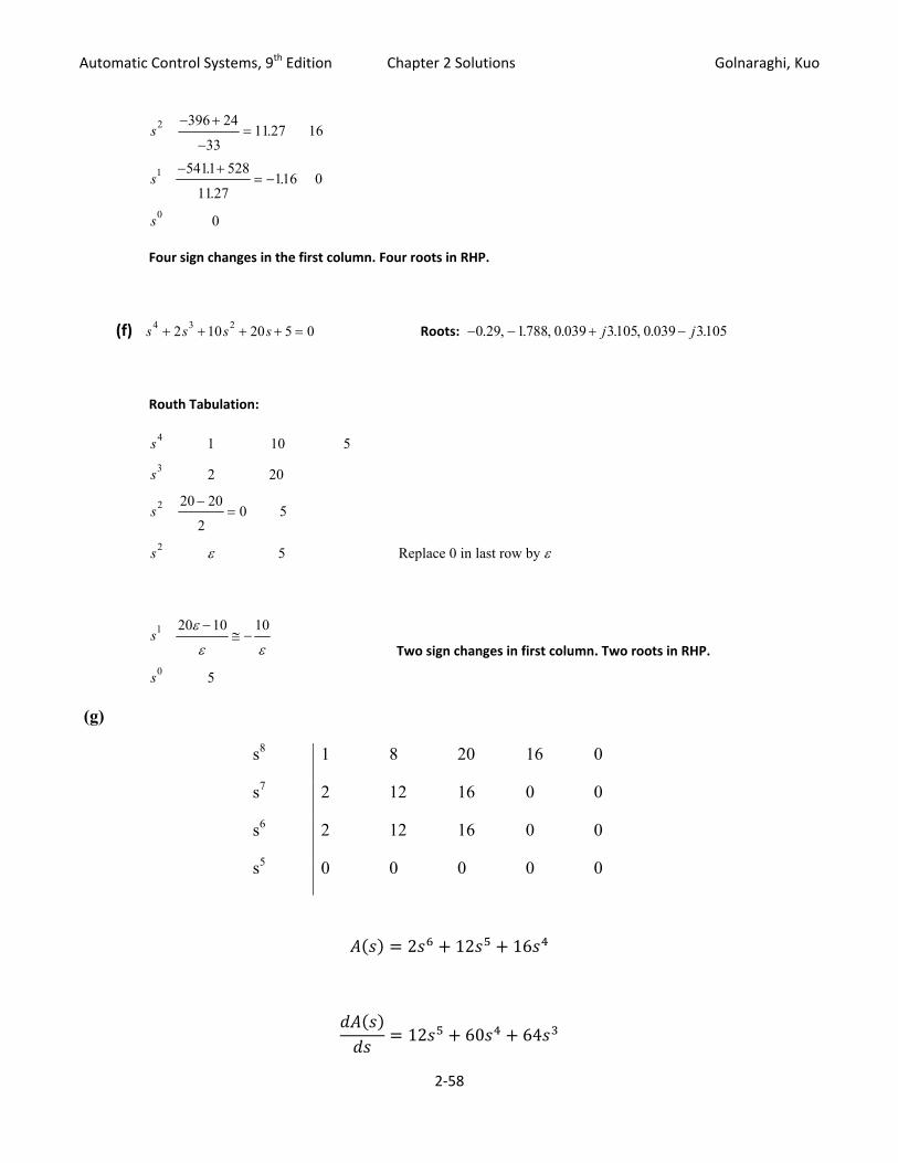
Automatic Control Systems, 9th Edition Chapter 2 Solutions Golnaraghi, Kuo (a) s s s s K4 3 225 15 20 0+ + + + =
Routh Tabulation:
s K
s
s K
4
3
2
1 15
25 20
375 20
2514.2
−=
s
KK K
s K K
1
0
284 25
14.220 176 20 176 0 1136
0
−= − − > <
>
. . or
K .
Thus, the system is stable for 0 < K < 11.36. When K = 11.36, the system is marginally stable. The
auxiliary equation is A s The solution of A(s) = 0 is s( ) . .= + =14.2 1136 02 s2 0 8= − . . The
frequency of oscillation is 0.894 rad/sec.
(b) s K s s K s4 3 22 1 10 0+ + + + + =( )
Routh Tabulation:
s
s K K K
sK K
K
K
KK
4
3
2
1 2 10
1 0
2 1 110 1
+ >
− −=
−>
s
K
KK
s
12
2
0
9 1
19 1
10
− −
−− − >
0
The conditions for stability are: K > 0, K > 1, and − − >9 12 0K . Since K 2 is always positive, the
last condition cannot be met by any real value of K. Thus, the system is unstable for all values of K.
2‐79

Automatic Control Systems, 9th Edition Chapter 2 Solutions Golnaraghi, Kuo
(c) s K s Ks3 22 2 10 0+ + + + =( )
Routh Tabulation:
s K
s K K
sK K
KK K
s
3
2
12
2
0
1 2
2 10 2
2 4 10
22 5
10
+ >
+ −
++ − > 0
−
The conditions for stability are: K > −2 and K K2 2 5 0+ − > or (K +3.4495)(K − 1.4495) > 0,
or K > 1.4495. Thus, the condition for stability is K > 1.4495. When K = 1.4495 the system is
marginally stable. The auxiliary equation is A s The solution is s( ) .4495 .= +3 102 = 0 s2 2 899= − . .
The frequency of oscillation is 1.7026 rad/sec.
(d) s s s K3 220 5 10 0+ + + =
Routh Tabulation:
s
s K
sK
K K
s K K
3
2
1
0
1 5
20 10
100 10
205 0 5 5 0 5 0 10
10 0
−= − − > <
>
. . or
K
The conditions for stability are: K > 0 and K < 10. Thus, 0 < K < 10. When K = 10, the system is
marginally stable. The auxiliary equation is The solution of the auxiliary A s s( ) .= + =20 100 02
equation is s2 5= − . The frequency of oscillation is 2.236 rad/sec.
2‐80

Automatic Control Systems, 9th Edition Chapter 2 Solutions Golnaraghi, Kuo
(e) s Ks s s K4 3 25 10 10+ + + + = 0
Routh Tabulation:
s K
s K K
sK
KK K
4
3
2
1 5 10
10 0
5 1010 5 10 0 2
>
−− > > or K
s
K
KK
K
K
K K
KK K
s K K
1
23
3
0
50 10010
5 1050 100 10
5 105 10
10 0
−−
−=
− −
−− − >
>
0
0
The conditions for stability are: K > 0, K > 2, and 5 10 3K K− − > .
Use Matlab to solve for k from last condition
>> syms k
>> kval=solve(5*k‐10+k^3,k);
>> eval(kval)
kval =
1.4233
‐0.7117 + 2.5533i
‐0.7117 ‐ 2.5533i
So K>1.4233.
Thus, the conditions for stability is: K > 2
2‐81

Automatic Control Systems, 9th Edition Chapter 2 Solutions Golnaraghi, Kuo (f) s s s s K4 3 212 5 5 0+ + + +. =
Routh Tabulation:
s K
s
s K
4
3
2
1 1
12 5 5
12 5 5
12 50 6
.
.
..
−=
s
KK K
s K K
1
0
3 12 5
0 65 20 83 5 20 83 0 0
0
−= − − > <
>
.
.. . .24 or
K
The condition for stability is 0 < K < 0.24. When K = 0.24 the system is marginally stable. The auxiliary
equation is The solution of the auxiliary equation is A s s( ) . .24 .= + =0 6 0 02 s2 0= − .4. The frequency of
oscillation is 0.632 rad/sec.
2-39)
The characteristic equation is Ts T s K s K3 22 1 2 5+ + + + + =( ) ( )
Routh Tabulation:
0
2−
s T K T
s T K T
3
2
2 0
2 1 5 1
+ >
+ >
/
s
T K KT
TK T T
s K K
1
0
2 1 2 5
2 11 3 4 2 0
5 0
( )( )( )
+ + −
+− + + >
>
The conditions for stability are: T > 0, K > 0, and . The regions of stability in the KT
T<
+
−
4 2
3 1
2‐82

Automatic Control Systems, 9th Edition Chapter 2 Solutions Golnaraghi, Kuo T‐versus‐K parameter plane is shown below.
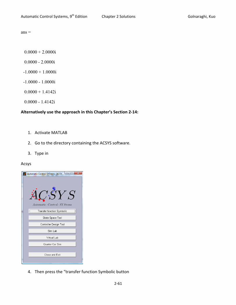
2‐40 Use the approach in this Chapter’s Section 2‐14:
1. Activate MATLAB
2. Go to the directory containing the ACSYS software.
3. Type in
Acsys
2‐83

Automatic Control Systems, 9th Edition Chapter 2 Solutions Golnaraghi, Kuo
2‐84
4. Then press the “transfer function Symbolic button.”
Automatic Control Systems, 9th Edition Chapter 2 Solutions Golnaraghi, Kuo
5. Enter the characteristic equation in the denominator and press the “Routh‐Hurwitz” push‐button.
RH =
[1, 50000, 24*k]
[600, k, 80*k]
[‐1/600*k+50000, 358/15*k, 0]
[ (35680*k‐1/600*k^2)/(‐1/600*k+50000), 80*k, 0]
[ 24*k*(k^2‐21622400*k+5000000000000)/(k‐30000000)/(35680*k‐1/600*k^2)*(‐1/600*k+50000), 0, 0]
[80*k, 0, 0]
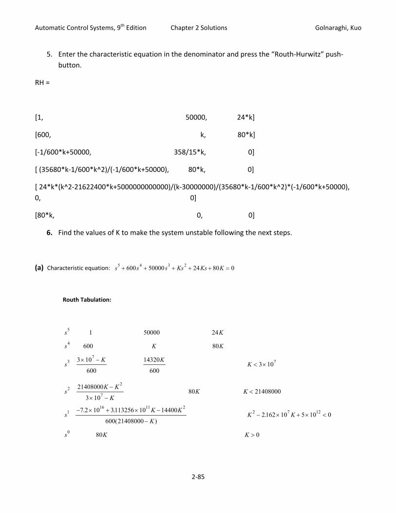
6. Find the values of K to make the system unstable following the next steps.
(a) Characteristic equation: s s s Ks Ks K5 4 3 2600 50000 24 80 0+ + + + + =
Routh Tabulation:
s K
s K K
sK K
K
5
4
37
7
1 50000 24
600 80
3 10
600
14320
6003 10
× −< ×
sK K
KK K
sK K
KK K
s K K
22
7
116 11 2
2 7
0
21408000
3 1080 21408000
7 10 3113256 10 14400
600(214080002162 10 5 10 0
80 0
−
× −<
− × + × −
−− × + × <
>
.2 .
). 12
2‐85

Automatic Control Systems, 9th Edition Chapter 2 Solutions Golnaraghi, Kuo
The so
Conditions for stability:
From the row: s3 K < ×3 107
From the row: s2 K < ×2 1408 107.
From the row: s1 K K K K2 7 12 52 162 10 5 10 0 2 34 10 2 1386 10 0− × + × < − × − × <. ( . )( . or 7 )
2 34 10 2 1386 105 7. .× < < ×K Thus,
From the row: K > 0 s0
Thus, the final condition for stability is: 2 34 10 2 1386 105 7. .× < < ×K
When rad/sec. K = ×2 34 105. ω = 10 6.
When rad/sec. K = ×2 1386 107. ω = 188 59.
(b) Characteristic equation: s K s Ks K3 22 30 200 0+ + + + =( )
Routh tabulation:
s K
s K K K
sK K
KK
s K K
3
2
12
0
1 30
2 200 2
30 140
24.6667
200 0
+ >
−
+>
>
Stability Condition: K > 4.6667
When K = 4.6667, the auxiliary equation is lution is .
−
=A s s( ) . .= +6 6667 933 333 02 s2 140= − .
The frequency of oscillation is 11.832 rad/sec.
(c) Characteristic equation: s s s K3 230 200 0+ + + =
2‐86

Automatic Control Systems, 9th Edition Chapter 2 Solutions Golnaraghi, Kuo
Th
Routh tabulation:
s
s K
sK
K
s K K
3
2
1
0
1 200
30
6000
306000
0
−<
>
Stabililty Condition: 0 6000< <K
When K = 6000, the auxiliary equation is e solution is A s s( ) .= + =30 6000 02 s2 200= − .
The frequency of oscillation is 14.142 rad/sec.
(d) Characteristic equation: s s K s K3 22 3) 1+ + + + + =( 0
Routh tabulation:
s K
s K
sK
K
s K K
3
2
1
0
1 3
2
5
305
1
+
+> −
> −
+1
+1
Stability condition: K > −1. When K = −1 the zero element occurs in the first element of the
row. Thus, there is no auxiliary equation. When K = −1, the system is marginally stable, and one s0
of the three characteristic equation roots is at s = 0. There is no oscillation. The system response
would increase monotonically.
2‐87

Automatic Control Systems, 9th Edition Chapter 2 Solutions Golnaraghi, Kuo
⎤⎥⎦
2‐42 State equation: Open‐loop system:
1 2 0
10 0 1
−= =⎡ ⎤ ⎡⎢ ⎥ ⎢⎣ ⎦ ⎣
A B
Closed‐loop system:
1 2
1 2
10 k k
−− =
− −
⎡ ⎤⎢ ⎥⎣ ⎦
A BK
Characteristic equation of the closed‐loop system:
( )2
2 1
1 2
1 21 20 2
10
ss s k s
k s k
−− + = = + − + − − =
− + +I A BK 2 0k k
Stability requirements:
Parameter plane:
2‐43) Characteristic equation of closed‐loop system:
( ) ( )3 2
3 2
1 2 3
1 0
0 1 3 4
4 3
s
s s s k s k
k k s k
−
− + = − = + + + + + =
+ + +
I A BK 1 0s k
t
& ( ) ( ) ( )x Ax Bt t u= +
& ( ) ( ) ( )x A BK xt t= −
k k2 21 0− > > or 1
120 2 0 20 21 2 2− − > < −k k k k or
2‐88
Automatic Control Systems, 9th Edition Chapter 2 Solutions Golnaraghi, Kuo
Routh Tabulation:
( )( )( )( )
3 2 1
0
1
3
2
2
3 1 3
1 3 2 1
3
3 4 0
1 4
3 +3>0 or 3
3 4
3k k k
s k
s k
s k k k k
k k ks
k+ + − >
+
+ >
+ + −
+
1 0k >
3−
Stability Requirements:
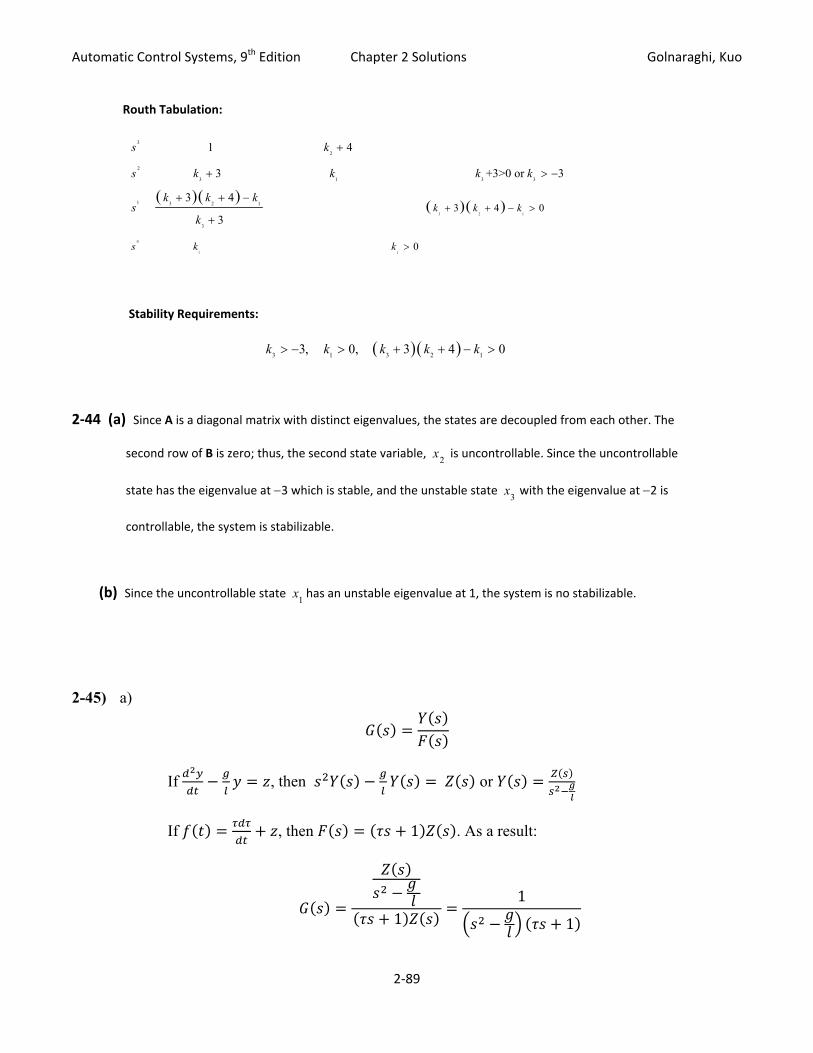
( )( )3 1 3 2 13, 0, 3 4 0k k k k k> − > + + − >
2‐44 (a) Since A is a diagonal matrix with distinct eigenvalues, the states are decoupled from each other. The
second row of B is zero; thus, the second state variable, is uncontrollable. Since the uncontrollable x2
state has the eigenvalue at −3 which is stable, and the unstable state with the eigenvalue at −2 is x3
controllable, the system is stabilizable.
(b) Since the uncontrollable state has an unstable eigenvalue at 1, the system is no stabilizable. x1
2-45) a)
, then or If
If , then . As a result:
2‐89
1
11
1

Automatic Control Systems, 9th Edition Chapter 2 Solutions Golnaraghi, Kuo
b1
1
As a result:
1
1
2
3 2
( )( ) ( ) ( )( ) (1 ( ) ( )) (( 1)( / ) )
( )( ( ( / ) 1) / )
p d
p d
p d
d p
K K sY s G s H sX s G s H s s s g l K K
K K ss g l s K s g l K
τ
τ τ
s+
= =+ + − +
+=
+ − + + − +
+
c) lets choose 10 0.1.
Use the approach in this Chapter’s Section 2‐14:
1. Activate MATLAB
2. Go to the directory containing the ACSYS software.
3. Type in
Acsys
2‐90
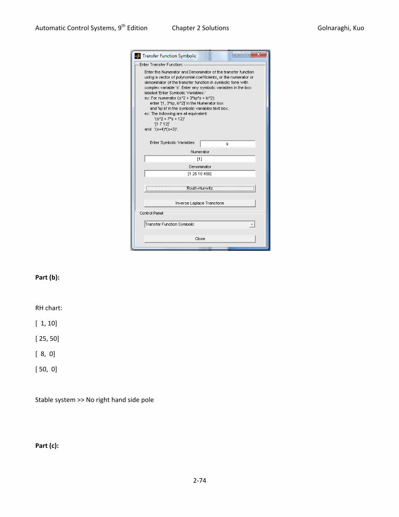
Automatic Control Systems, 9th Edition Chapter 2 Solutions Golnaraghi, Kuo
2‐91
4. Then press the “transfer function Symbolic button.”
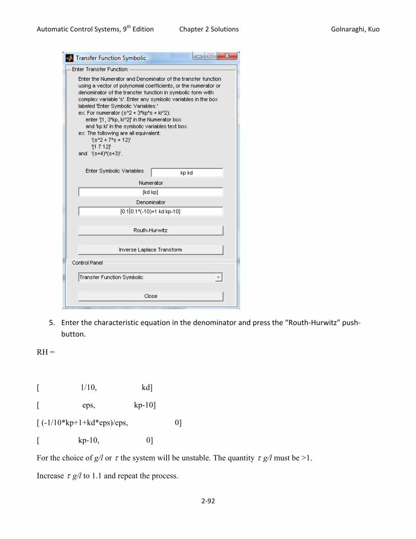
Automatic Control Systems, 9th Edition Chapter 2 Solutions Golnaraghi, Kuo
5. Enter the characteristic equation in the denominator and press the “Routh‐Hurwitz” push‐button.
RH =
[ 1/10, kd]
[ eps, kp-10]
[ (-1/10*kp+1+kd*eps)/eps, 0]
[ kp-10, 0]
For the choice of g/l or τ the system will be unstable. The quantity τ g/l must be >1.
Increase τ g/l to 1.1 and repeat the process.
2‐92
Automatic Control Systems, 9th Edition Chapter 2 Solutions Golnaraghi, Kuo
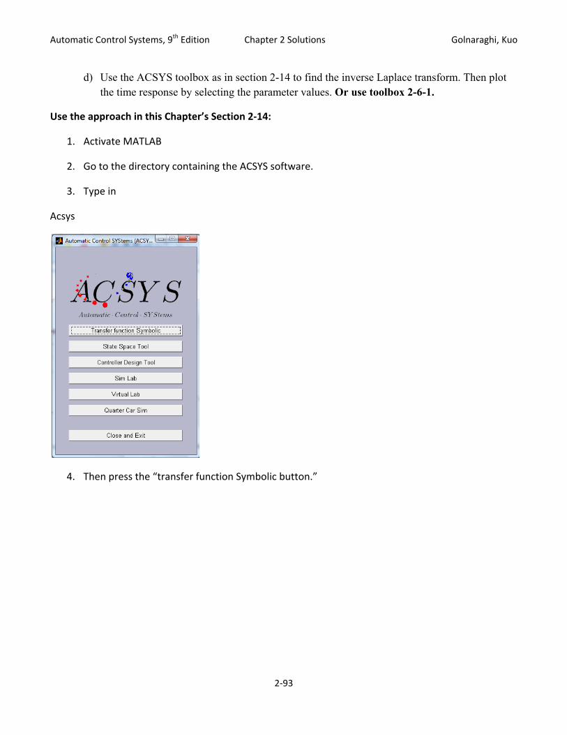
d) Use the ACSYS toolbox as in section 2-14 to find the inverse Laplace transform. Then plot the time response by selecting the parameter values. Or use toolbox 2-6-1.
Use the approach in this Chapter’s Section 2‐14:
1. Activate MATLAB
2. Go to the directory containing the ACSYS software.
3. Type in
Acsys
4. Then press the “transfer function Symbolic button.”
2‐93

Automatic Control Systems, 9th Edition Chapter 2 Solutions Golnaraghi, Kuo
5. Enter the characteristic equation in the denominator and press the “Inverse Laplace Transform” push‐button.
----------------------------------------------------------------
Inverse Laplace Transform
----------------------------------------------------------------
2‐94
Automatic Control Systems, 9th Edition Chapter 2 Solutions Golnaraghi, Kuo
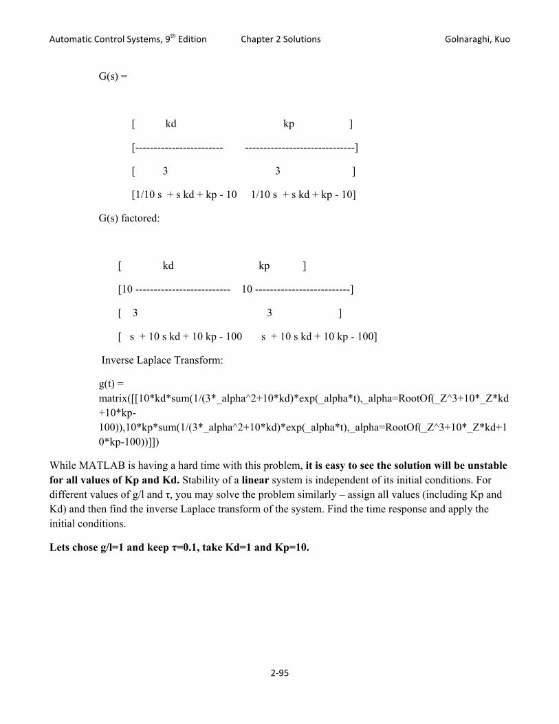
G(s) =
[ kd kp ]
[------------------------ ------------------------------]
[ 3 3 ]
[1/10 s + s kd + kp - 10 1/10 s + s kd + kp - 10]
G(s) factored:
[ kd kp ]
[10 -------------------------- 10 --------------------------]
[ 3 3 ]
[ s + 10 s kd + 10 kp - 100 s + 10 s kd + 10 kp - 100]
Inverse Laplace Transform:
g(t) = matrix([[10*kd*sum(1/(3*_alpha^2+10*kd)*exp(_alpha*t),_alpha=RootOf(_Z^3+10*_Z*kd+10*kp-100)),10*kp*sum(1/(3*_alpha^2+10*kd)*exp(_alpha*t),_alpha=RootOf(_Z^3+10*_Z*kd+10*kp-100))]])
While MATLAB is having a hard time with this problem, it is easy to see the solution will be unstable for all values of Kp and Kd. Stability of a linear system is independent of its initial conditions. For different values of g/l and τ, you may solve the problem similarly – assign all values (including Kp and Kd) and then find the inverse Laplace transform of the system. Find the time response and apply the initial conditions.
Lets chose g/l=1 and keep τ=0.1, take Kd=1 and Kp=10.
2‐95

Automatic Control Systems, 9th Edition Chapter 2 Solutions Golnaraghi, Kuo
2
3 2 3 2
( )( ) ( ) ( )( ) (1 ( ) ( )) (( 1)( / ) )
(10 ) (10 )(0.1 (0.1( 1) 1) 1 10) (0.1 0.9 9)
p d
p d
K K sY s G s H sX s G s H s s s g l K K s
s ss s s s s
τ
s
+= =
+ + − + +
+ += =
+ − + + − + + + +
Using ACSYS:
RH =
[ 1/10, 1]
[ 9/10, 9]
[ 9/5, 0]
[ 9, 0]
Hence the system is stable
----------------------------------------------------------------
Inverse Laplace Transform
----------------------------------------------------------------
G(s) =
s + 10
-------------------------
3 2
1/10 s + 9/10 s + s + 9
2‐96

Automatic Control Systems, 9th Edition Chapter 2 Solutions Golnaraghi, Kuo
G factored:
Zero/pole/gain:
10 (s+10)
-----------------
(s+9) (s^2 + 10)
Inverse Laplace Transform:
g(t) = -10989/100000*exp(-2251801791980457/40564819207303340847894502572032*t)*cos(79057/25000*t)+868757373/250000000*exp(-2251801791980457/40564819207303340847894502572032*t)*sin(79057/25000*t)+10989/100000*exp(-9*t)
Use this MATLAB code to plot the time response:
for i=1:1000
t=0.1*i;
tf(i)=‐10989/100000*exp(‐2251801791980457/40564819207303340847894502572032*t)*cos(79057/25000*t)+868757373/250000000*exp(‐2251801791980457/40564819207303340847894502572032*t)*sin(79057/25000*t)+10989/100000*exp(‐9*t);
end
figure(3)
plot(1:1000,tf)
2‐97

Automatic Control Systems, 9th Edition Chapter 2 Solutions Golnaraghi, Kuo
2‐52) USE MATLAB
syms t
f=5+2*exp(‐2*t)*sin(2*t+pi/4)‐4*exp(‐2*t)*cos(2*t‐pi/2)+3*exp(‐4*t)
F=laplace(f)
cltF=F/(1+F)
f =
5+2*exp(‐2*t)*sin(2*t+1/4*pi)‐4*exp(‐2*t)*sin(2*t)+3*exp(‐4*t)
F =
(8*s^3+44*s^2+112*s+160+8*2^(1/2)*s^2+16*2^(1/2)*s+2^(1/2)*s^3)/s/(s^2+4*s+8)/(s+4)
cltF =
2‐98
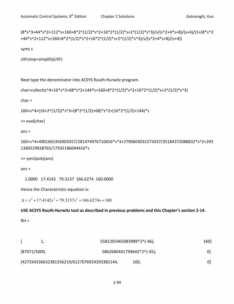
Automatic Control Systems, 9th Edition Chapter 2 Solutions Golnaraghi, Kuo (8*s^3+44*s^2+112*s+160+8*2^(1/2)*s^2+16*2^(1/2)*s+2^(1/2)*s^3)/s/(s^2+4*s+8)/(s+4)/(1+(8*s^3+44*s^2+112*s+160+8*2^(1/2)*s^2+16*2^(1/2)*s+2^(1/2)*s^3)/s/(s^2+4*s+8)/(s+4))
syms s
cltFsimp=simplify(cltF)
Next type the denominator into ACSYS Routh‐Hurwitz program.
char=collect(s^4+16*s^3+68*s^2+144*s+160+8*2^(1/2)*s^2+16*2^(1/2)*s+2^(1/2)*s^3)
char =
160+s^4+(16+2^(1/2))*s^3+(8*2^(1/2)+68)*s^2+(16*2^(1/2)+144)*s
>> eval(char)
ans =
160+s^4+4901665356903357/281474976710656*s^3+2790603031573437/35184372088832*s^2+2931340519928765/17592186044416*s
>> sym2poly(ans)
ans =
1.0000 17.4142 79.3137 166.6274 160.0000
Hence the Characteristic equation is:
4 3 217.4142 79.3137 166.6274 160s s s sΔ = + + + +
USE ACSYS Routh‐Hurwitz tool as described in previous problems and this Chapter’s section 2‐14.
RH =
[ 1, 5581205465083989*2^(‐46), 160]
[87071/5000, 5862680441794645*2^(‐45), 0]
[427334336632381556219/6127076924293382144, 160, 0]
2‐99
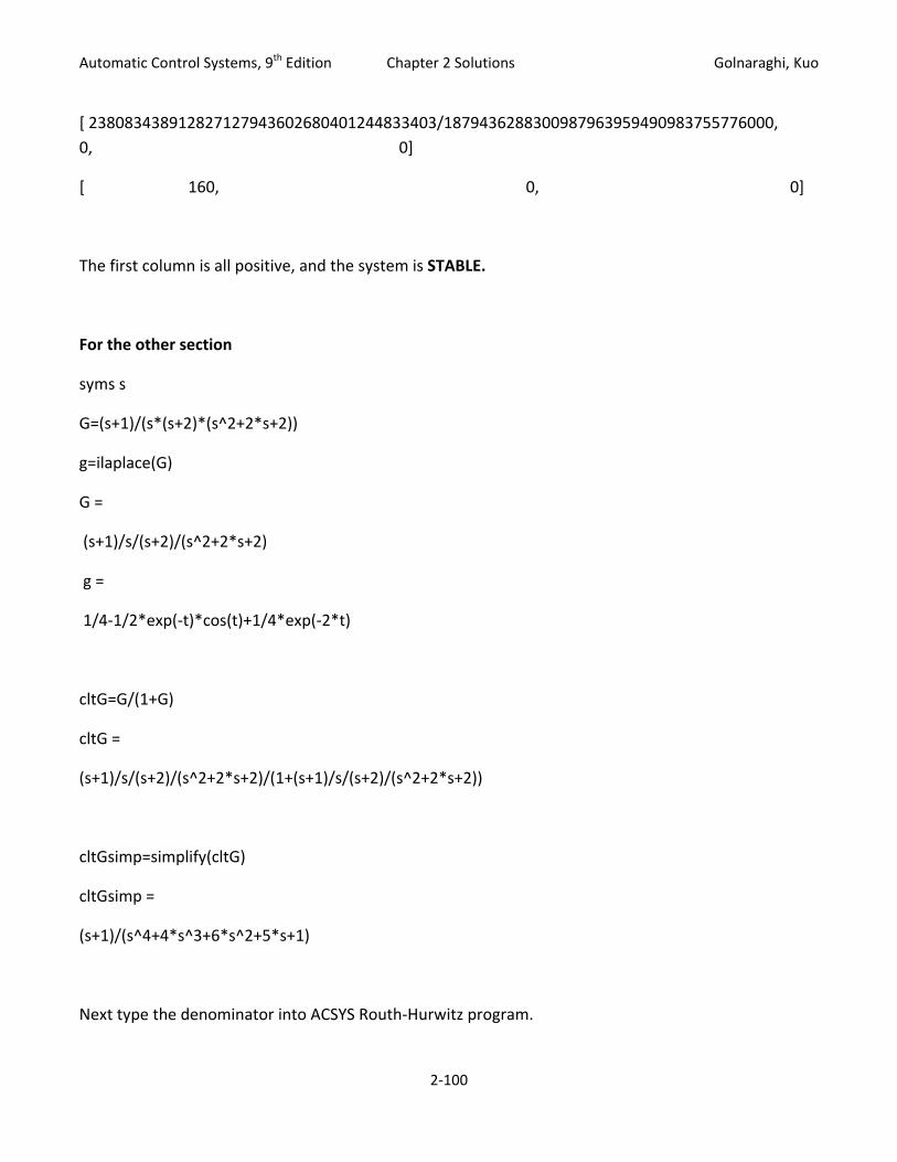
Automatic Control Systems, 9th Edition Chapter 2 Solutions Golnaraghi, Kuo [ 238083438912827127943602680401244833403/1879436288300987963959490983755776000, 0, 0]
[ 160, 0, 0]
The first column is all positive, and the system is STABLE.
For the other section
syms s
G=(s+1)/(s*(s+2)*(s^2+2*s+2))
g=ilaplace(G)
G =
(s+1)/s/(s+2)/(s^2+2*s+2)
g =
1/4‐1/2*exp(‐t)*cos(t)+1/4*exp(‐2*t)
cltG=G/(1+G)
cltG =
(s+1)/s/(s+2)/(s^2+2*s+2)/(1+(s+1)/s/(s+2)/(s^2+2*s+2))
cltGsimp=simplify(cltG)
cltGsimp =
(s+1)/(s^4+4*s^3+6*s^2+5*s+1)
Next type the denominator into ACSYS Routh‐Hurwitz program.
2‐100
Automatic Control Systems, 9th Edition Chapter 2 Solutions Golnaraghi, Kuo
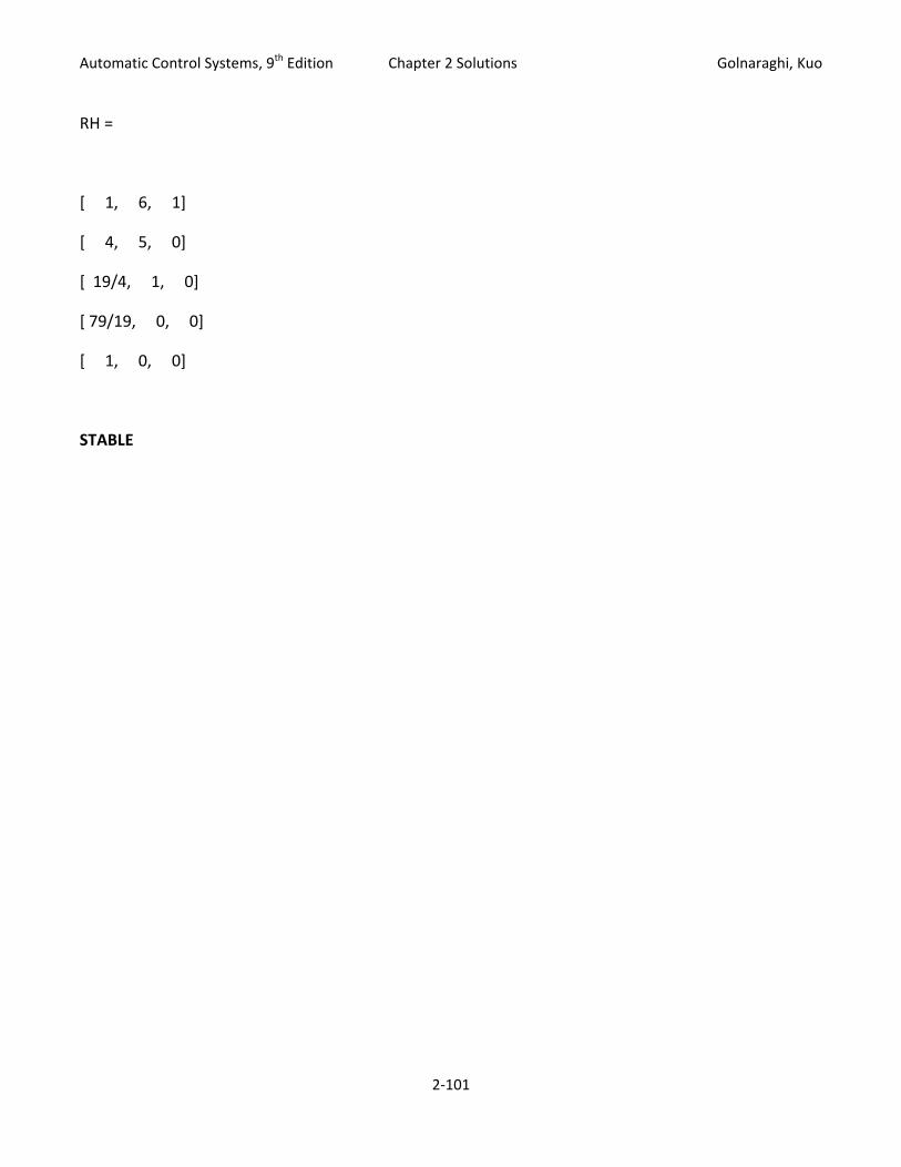
2‐101
RH =
[ 1, 6, 1]
[ 4, 5, 0]
[ 19/4, 1, 0]
[ 79/19, 0, 0]
[ 1, 0, 0]
STABLE