2 - higher-order, cascaded, active...

ECE 6414: Continuous Time Filters (P. Allen) - Chapter 2 Page 2-1

2 - HIGHER-ORDER, CASCADED, ACTIVE FILTERS

In the previous chapter we have shown how to design second-order active filters.

However, most filter applications require an order higher than two. The objective of this

section will be to show how to use the first- and second-order filters to achieve higher

order filters. We shall also introduce a general, second-order stage called the biquad. The

biquad is useful as a general component in filter realizations.

Higher-order active filters as presented in this section is strictly a design activity. We

will begin by understanding how a filter is specified. A great deal of tabular information is

available as a starting point for the design. This tabular information is generally presented

in the form of a normalized low-pass filter as shown in Fig. 2-1.

Low-Pass,NormalizedFilter with a passband of 1 rps and an impedance of 1 ohm.

Denormalize the Filter

Realization

Cascade of First- and/or Second-Order

Stages

First-OrderReplacement

of LadderComponents

Frequency Transform the Roots to HP,

BP, or BS

Frequency Transform the L's and C's to

HP, BP, or BS

Normalized LP Filter

RootLocations

Normalized Low-Pass

RLC Ladder Realization

Figure 2-1 - General design approach for active filters of Chapters 2 and 3.

Two design approaches are used design higher-order active filters. One is based on

realizing the root locations of the filter with cascaded first- and second-order stages and the

second is based on replacing components of a passive RLC ladder filter with first-order

stages. We will postpone our discussion of ladder filter design to the next section. If the

filter is to be other than low-pass, then it is necessary to transform the filter design to a

high-pass (HP), bandpass (BP), or bandstop (BS). The last step in higher-order, low-pass

filter design is to denormalize the design to achieve the actual performance specifications.

The subject of active filters is an extensive one and encompasses more material than

can be presented in this section. We shall attempt to give an overview and illustrate some

of the basic concepts and design procedures. For more information, the reader is referred

ECE 6414: Continuous Time Filters (P. Allen) - Chapter 2 -2

to the many excellent texts that cover this subject in much more detail†. In the simulation

part of this section, we shall illustrate one of the computer-aided design approaches

presently available for the design of active filters.

Ideal Filters

Filters are generally classified by their magnitude response in the frequency domain

only. However, there are some filters, which will not be considered here, that are

characterized by both their magnitude and phase response. The magnitude response of an

ideal filter will be divided into two types of regions. One region has a gain of unity and is

called the passband. Even though filters can have gains greater or less than unity in the

passband, we shall consider the passband gain unity for purposes of simplicity. The

second region has a gain of zero and is called the stopband. We shall also assume that the

ideal filter can have the passband adjacent to the stopband and that ωT is the frequency

where the transition is made from one band to the other.

Fig. 2-2 shows the four categories of filters that we shall consider. The first category

is called a low-pass filter and has a gain of 1 from 0 to ωT and a gain of zero for all

frequencies greater than ωT. The ideal low-pass filter is illustrated by Fig. 2-2a. The

magnitude response of this filter is given as

TLP(jω)| = 1 0≤ω≤ωT

0 ωT<ω<∞ . (2-1)

† A. Budak, Passive and Active Network Analysis and Synthesis, Houghton Mifflin Co., Boston, 1974. J.L. Hilburn and D.E. Johnson, Manual of Active Filter Design, McGraw-Hill Book Co., NY, 1973.

L.P. Huelsman and P.E. Allen, Introduction to the Theory and Design of Active Filters, McGraw-Hill Book Co., NY, 1980.R. Schaumann, M. S. Ghausi, and K.R. Laker, Design of Analog Filters, Prentice-Hall, Englewood Cliffs, NJ, 1990.A.S. Sedra and P.O. Brackett, Filter Theory and Design: Active and Passive, Matrix Publishers Inc., Portland, OR, 1977.M.E. Van Valkenburg, Introduction to Modern Network Synthesis, John Wiley & Sons, Inc. NY, 1960.L. Weinburg, Network Analysis and Synthesis, McGraw-Hill Book Co., 1962, R.E. Krieger Publishing Co., Huntington, NY, 1975.A.I. Zverev, Handbook of Filter Synthesis, John Wiley & Sons, Inc., NY, 1967.


1

00 ωT

ω (rps)

TLP(jω)

1

00 ωT

ω (rps)

THP(jω)

1

00

ω (rps)

TBP(jω)

ωT1 ωT2

1

00

ω (rps)

TBS(jω)

ωT1 ωT2

(a.) (b.)

(c.) (d.)

Figure 2-2 - Ideal magnitude responses of (a.) low-pass, (b.) high-pass, (c.) bandpass,

and (d.) bandstop filter.

The second category of ideal filter is the high-pass filter and has a gain of 0 from 0 to

ωT and a gain of 1 for all frequencies greater than or equal to ωT. The ideal high-pass filter

is shown in Fig. 2-2b. The magnitude response of the high-pass filter is given as

THP(jω)| = 0 0≤ ω< ωT

1 ωT≤ ω< ∞ . (2-2)

The third category of ideal filters is the bandpass filter and has a gain of 1 between the

frequencies of ωT1 and ωT2 and a gain of zero elsewhere. The magnitude response of an

ideal bandpass filter is shown in Fig. 2-2c and is mathematically expressed as

TBP(jω)| = 0 0≤ ω< ωT 1

1 ωT1≤ω<ωT 2

0 ωT 2 < ω< ∞ . (2-3)

The fourth and last category of ideal filters is the bandstop filter and has a gain of 0

between the frequencies of ωT1 and ωT2 and a gain of 1 elsewhere. The magnitude


response of an ideal bandpass filter is shown in Fig. 2-2d and is mathematically expressed

as

TBP(jω)| = 1 0≤ ω< ωT 1

0 ωT1≤ω<ωT 2

1 ωT 2 < ω< ∞ . (2-4)

The phase response of each of these ideal filters is exactly the same. It is given as

Arg[T(jω)] = -ωTd , 0 ≤ ω ≤ ∞ . (2-5)

We see the ideal phase shift is a straight line passing through 0 degrees at ω = 0 and having

a slope of -Td. Because the time delay of a filter is equal to the negative derivative of the

phase shift with respect to frequency, Td is called the time delay of the filter and is constant

for all frequencies.

Practical Filters

Practical filters cannot have a continuous band of zero gain nor can they have an

instantaneous transition from the passband to the stopband. Consequently, we need to

extend our ideal filter specifications to include practical filters. This is done by defining the

filter magnitude response in terms of constraints separated by finite-width transition

regions. Fig. 2-3 shows the magnitude specifications for the four types of filters that can

be realized by active and/or passive circuits.

The low-pass filter specification of Fig. 2-3a has been divided into three frequency

regions. From 0 to ωPB the magnitude must be between 1 and TPB. This is passband

region. From ωSB to infinity, the magnitude must be less than TSB. This is the stopband

region. The region between ωPB and ωSB is called the transition region. The magnitude of

the filter is unspecified in this region, although a good approximation would be expected to

closely follow a straight line drawn from point A to point B. Any filter design which stays

within the shaded regions and approximates a straight-line from A to B in the transition

region will satisfy the filter specifications. The line shown on Fig. 2-3a is an example of

one possible filter realization whose magnitude response would satisfy the specifications.


It is not necessary that the magnitude response oscillate as shown, but this characteristic

permits practical filters to have a smaller transition region than filter realizations whose

slope is monotonic.

(a.) (b.)

(c.) (d.)

0 ωSBωPB

1

0 ω (rps)

TLP(jω)

TPB

TSB

TransitionRegion

A

B

One possiblefilter realization

ωPB

THP(jω)

1

00

ω (rps)

TPB

TSB

ωSB

TransitionRegionA

BOne possiblefilter realization

1

00

ω (rps)

TBP(jω)

ωPB1ωPB2 ωSB2ωSB1

TPB

TSB A

B C

D

One possiblefilter realizationLower

TransitionRegion Upper Transi-

tion Region

0ω (rps)

TBS(jω)

1

00

ω (rps)ωPB1 ωPB2ωSB2ωSB1

TPB

TSB

A

B

C

D


LowerTransitionRegion

Upper Transi-tion Region

Figure 2-3 - Practical magnitude responses of (a.) low-pass, (b.) high-pass, (c.) bandpass,

and (d.) bandstop filter.

Figs. 2-3b through 2-d are practical magnitude specifications for the high-pass,

bandpass, and bandstop filters, respectively. In each case, the magnitude of the filter must

fall within the shaded areas. The magnitude of the filter in the transition region(s) should

approximate a straight-line through points A and B or C and D, in the case of the bandpass

and bandstop filters.

In order to simplify the filter design procedure, all filter design begins with a

normalized, low-pass filter specification. The normalized low-pass filter is a structure from

which all other filters can be derived by denormalization or transformation. The low-pass

filter is normalized so that ωPB of Fig. 2-3a is unity. The low-pass filter has also been

normalized to an impedance level of 1 ohm. Fig. 2-1 illustrates the low-pass, normalized


filter is the starting point of all filter design. The normalizations used in the low-pass, filter

are defined as follows. The normalized frequency variable, sn, is defined as

sn = s

ωPB (2-6)

where we use sn to indicate the frequency normalized complex variable. The normalization

impedance, Zn, used in the low-pass filter is defined as

Zn = Zzo

(2-7)

where Z is the unnormalized impedance and zo is a unitless impedance scaling constant. In

RLC passive filters, the impedance level is important. However, in active filter design, the

impedance denormalization amounts to a simple impedance scaling constant. We must

remember that the normalization definitions in Eqs. (2-6) and (2-7) apply only to the low-

pass filter of Fig. 2-3a.

Often, the entire design of an active filter is done using the normalized complex

frequency variable, sn, and the normalized impedance, Zn. At the end of the design

procedure, as indicated in Fig. 2-1, the filter is denormalized to achieve the desired

frequency range and to scale the passive component to values which are more convenient.

This denormalization is simply the inverse of Eqs. (2-6) and (2-7). Table 2-1 gives the

influence of the frequency and impedance denormalization is illustrated on the normalized

passive components and the normalized root locations of a filter.

Example 2-1 - Appli cation of the Denormalizing Factors to the Low-Pass Filter

Suppose that a normalized, second-order, low-pass filter is characterized by the

circuit of Fig. 2-4 or by the following pole locations pn1, pn2 = -1

2 ± j

1

2 .

Find the denormalized circuit and pole locations if the filter is to have a passband frequency

of 1 kHz and the resistors in the realization should be 10 kΩ.


Ln= 2H

+

-

+

-

Vin(sn) Vout(sn)Cn=1/ 2F

Rn=1Ω

Figure 2-4 - A normalized, second-order, low-pass filter.

Solution

From the information given, ωPB is 2πx103 rps. zo is 104 because the normalized 1

Ω in Fig. 2-4 is to become 10 kΩ. Therefore, the denormalized pole locations are

p1, p2 = - (0.707)(2πx103) ±j (0.707)(2πx103) = -4,443 ± j4,443 rps .

The denormalized components of Fig. 2-4 become

L =104 26283.2 = 2.251 H,

C = 1

2(6283.2)(104) = 0.1125 nF,

and

R = 10 kΩ.

Table 2-1 - Influence of the frequency and impedance denormalizations on the passive

components and root locations of a filter.

Denormalization↓

DenormalizedResistance, R

DenormalizedCapacitance, C

DenormalizedInductance, L

DenormalizedPole, p, or

Zero, z

Frequency -s = ωPBsn

= ωPBp

R = RnC =

Cn

ωPB L =

Ln

ωPB

p = ωPBpn

z = ωPBzn

Impedance -Z = zoZn R = zoRn

C = Cnzo

L = zoLn

p = pnz = zn

Frequency andImpedance -

Z(s) =zoZn(ωPBsn)

R = zoRnC =

Cn

zoωPB L =

zoLn

ωPB p = ωPBpn

z = ωPBzn


Attenuation Viewpoint of Practical Filter Specifications

Fig. 2-5a shows the specifications of a low-pass filter where the vertical axis has

been plotted in terms of dB. If we normalize the frequency axis by ωPB, then the

normalized passband frequency is now 1 rps and the normalized stopband frequency, Ωn,

is given as

Ωn = ωSB

ωPB . (2-8)

The realizations of this normalized, low-pass filter must remain in the shaded areas and

approximate a straight-line drawn through points A and B in the transition region. A

possible filter realization is shown on Fig. 2-5a.

(a.) (b.)

0 dBA

B


Ωn1

log10 ωnAPB dB

ASB dB

log10 ALP(jωn)

0 dB

A

B


Ωn1 log10 ωn

log10 TLP(jωn)

TPB dB

TSB dB

Figure 2-5 - Normalized, low-pass filter. (a.) Gain in dB. (b.) Attenuation in dB.

Because we have normalized the gain of the low-pass filter to unity, the dB values are

all negative. Sometimes, it is convenient to view the normalized, low-pass filter from

attenuation which is the reciprocal of gain. An attenuation plot in dB for the normalized,

low-pass filter of Fig. 2-5a is shown in Fig. 2-5b. In some references, APB is called

AMAX and ASB is called AΩ or AMIN.

The specification for the normalized, low-pass filter is completely described by three

parameters. These parameters are TPB, TSB, and Ωn or APB, ASB, and Ωn. Once these

parameter values are known, then we must determine the order of the filter necessary to

satisfy the specification. However, the order is determined by the type of filter

approximation used to realize the specifications. While there are numerous filter


approximations, we shall discuss two of the more popular ones next. They are the

maximally flat magnitude or Butterworth approximation and the equal passband ripple or

Chebyshev approximation.

Normalized, Low-Pass, Butterworth Filter Approximation

One of the more useful filter approximations to the normalized low-pass filter is called

the Butterworth† filter approximation. The magnitude of the Butterworth filter

approximation is maximally flat at low frequencies (ω→0) and monotonically rolls off to a

value approaching zero at high frequencies (ω→∞). The magnitude of the normalized,

Butterworth, low-pass filter approximation can be expressed as

| |TLPn(jωn) = 1

1 + ε2 ω2 N

n

(2-9)

where N is the order of the filter approximation and ε is defined in Fig. 2-6. Fig. 2-6

shows the magnitude response of the Butterworth filter approximation for several values of

N.

Normalized Frequency, ωn

0 0.5 1 1.5 2 2.5 30

0.2

0.4

0.6

0.8

1

TLPn(jωn)

A

N=5

N=2N=4

N=3N=6

N=8

N=10

1

1+ε2

Figure 2-6 - Magnitude response of a normalized Butterworth low-pass filter

approximation for various orders, N, and for ε = 1.

† S. Butterworth was a British engineer who described this type of filter approximation in conjunction with

electronic amplifiers in his paper "On The Theory of Filter Amplifiers," Wireless Engineer, vol. 7, 1930.


The shaded area on Fig. 2-6 corresponds to the shaded area in the passband region of

Figs. 2-3a and 2-5a. It is characteristic of all filter approximations that they pass through

the point A as illustrated on Fig. 2-6. The value of ε can be used to adjust the width of the

shaded area in Fig. 2-6. Normally, Butterworth filter approximations are given for an ε of

unity as illustrated on Fig. 2-6. We see from Fig. 2-6 that the higher the order of the filter

approximation, the smaller the transition region for given value of TSB. For example, if

TPB = 0.707 (ε = 1), TSB = 0.1 and Ωn = 1.5 (illustrated by the both shaded areas of Fig.

2-6), then the order of the Butterworth filter approximation must be 6 or greater to satisfy

the specifications. Note that the order must be an integer which means that even though N

= 6 exceeds the specification it must be used because N = 5 does not meet the specification.

The magnitude of the Butterworth filter approximation at ωSB can be expressed from Eq.

(2-9) as

TLPn

jωSB

ωPB = |TLPn(jΩn)| = TSB =

1

1 + ε2 Ω2 N

n

. (2-10)

This equation is useful for determining the order required to satisfy a given filter

specification. Often, the filter specification is given in terms of dB. In this case, Eq. (2-

10) is rewritten as

20 log10(TSB) = TSB (dB) = -10 log10 1 + ε2 Ω2 N

n . (2-11)

Example 2-2 - Determining the Order of A Butterworth Filter Approximation

Assume that a normalized, low-pass filter is specified as TBP = -3dB, TSB = -20 dB,

and Ωn = 1.5. Find the smallest integer value of N of the Butterworth filter approximation

which will satisfy this specification.

Solution

TBP = -3dB corresponds to TBP = 0.707 which implies that ε = 1. Thus, substituting

ε = 1 and Ωn = 1.5 into Eq. (2-11) gives

TSB (dB) = - 10 log10( )1 + 1.52 N .


Substituting values of N into this equation gives TSB = -7.83 dB for N = 2,

-10.93 dB for N = 3, -14.25 dB for N = 4, -17.68 dB for N = 5, and -21.16 dB for N =

6. Thus, N must be 6 or greater to meet the filter specification.

Once, the order of the Butterworth filter approximation is known, we must next find

the normalized root locations. Of course, all zeros are at infinity because the realization is

low-pass. The poles depend on the value of ε. For ε = 1, the pole locations are on a unit

circle. The normalized poles are designated as pkn = σkn + jωkn and are given as

σkn = - sin

(2k - 1)π

2N and ωkn = cos

(2k - 1)π

2N , k = 1,2,3,···, N . (2-12)

To help illustrate this formula, the poles for fifth-order, Butterworth filter approximation

have been evaluated and are given in Table 2-2. Figure 2-7 shows the pole locations for

the fifth-order, Butterworth filter approximation. It can be shown that these poles are

angularly spaced by an amount of π/N (36° for N = 5).

k σkn = - sin

(2k - 1)π

2N ωkn = cos

(2k - 1)π

2N

1 -0.3090 rps 0.9511 rps

2 -0.8090 rps 0.5878 rps

3 -1.0000 rps 0.0000 rps

4 -0.8090 rps -0.5878 rps

5 -0.3090 rps -0.9511 rps

Table 2-2 - Normalized pole locations for a fifth-order, Butterworth filter approximation.

Cascade Realization of Butterworth Filter Approximations

It is important to realize that while the Butterworth filter approximation is monotonic,

the individual pole pairs are not. For example, let us write the normalized transfer function

of the fifth-order example of Table 2-2 into the product of two, second-order terms and

one, first-order terms. The filter transfer function is written as

TLPn(sn) =

p3n

sn+p3n

p1np5n

(sn+p1n)(sn+p5n)

p2np4n

(sn+p2n)(sn+p4n) (2-13)


where we have grouped the complex-conjugate poles into second-order terms. Substituting

the values of Table 2-2 into Eq. (2-13) gives

TLPn(sn) = T1(sn)T2(sn)T3(sn) =

1

sn+1

1

s2n+0.6180sn+1

1

s2n+1.6180sn+1

. (2-14)

The contributions of the first-order term, T1(sn), and the two second-order terms, T2(sn)

and T3(sn), can be illustrated by plotting each one separately and then taking the products

of all three. Fig. 2-8 shows the result. Interestingly enough, we see that the magnitude of

T2(sn) has a peak that is about 1.7 times the gain of the fifth-order filter at low frequencies.

If we plotted Fig. 2-8 with the vertical scale in dB, we could identify the Q by comparing

the results with the normalized second-order, magnitude responses of Fig. 1-6a.

Consequently, all filter approximations that are made up from first-order and/or second-

order products do not necessarily have the properties of the filter approximation until all the

terms are multiplied (added on a dB scale).

jωn

σn1

j1

-j1

-1 -0 8090 -0 3090

j0.9511

j0.5878

-j0 5878

-j0.9511

p1n

p2n

p3n

p4n

p5n

Figure 2-7 - Example of the normalized pole locations for a fifth-order, normalized

Butterworth filter approximation.


0

0.5

1

1.5

2

0 0.5 1 1.5 2 2.5 3

T1(jωn)

T2(jωn)

T3(jωn)

(jωnTLPn )M

agni

tude


Figure 2-8 - Individual magnitude contributions of a fifth-order, Butterworth filter

approximation.

Now we see how the Butterworth filter approximation can be realized by the

cascading of second-order stages and, at most, one-first order stage. The design procedure

is stated as follows:

1.) From TPB, TSB, and Ωn (or APB, ASB, and Ωn) determine the required order of

the Butterworth filter approximation using Eq. (2-10) or Eq. (2-11).

2.) From Eq. (2-12) find the normalized poles of the approximation.

3.) Group the complex-conjugate poles into second-order realizations. For odd-

order realizations there will be one first-order term of the form 1/(sn+1).

4.) Realize each of the second-order terms using the active filters of Sec. 1. Realize

the first-order section (if any) by the first-order low-pass circuits of Sec. 4.2.

5.) Cascade the realizations in the order from input to output of the lowest-Q stage

first (first-order stages generally should be first).

6.) Denormalize to the desired passband frequency and denormalize the impedances

if desired.

Step 5 covers an aspect we have not considered and that is the order of the stages. The

principle behind the ordering suggested in step 5 is to prevent one stage from being

overdriven. Consider the fifth-order filter of Fig. 2-8 to illustrate this principle. If the


frequency applied to the filter is at the passband (ωn = 1), the gain of T2(sn) is about 1.6

while the gain of T1(sn) is 0.707 and T3(sn) is 0.6. If the order were T2, T1, and T3 and

the amplitude of the sinusoid at ωn = 1 was 1V, the output of the first stage (T2) would be

1.6V, the output of the second stage (T1) would be 1.13V, and finally the output of the

third stage (T3) would be 0.707. If the input signal is too large, or the power supply

voltages too small, the first and possibly the second stages may saturate or clip. However,

if we put the stages in the order of T1, T3, and T2 or T3, T1 and T2, saturation will not

occur and one can achieve maximum signal amplitude. Let us illustrate the cascade design

approach with an example.

Example 2-3 - Design of a Fifth-Order, Low-Pass Butterworth Filter

Design a cascade, active filter realization for a Butterworth filter approximation to the

filter specifications of APB = 3dB, ASB = 30 dB, fPB = 1 kHz, and fSB = 2 kHz. Give a

schematic and component values for the realization using the negative feedback, second-

order, low-pass active filter of Fig. 1-14 and any first-order stage that may be necessary.

Solution

First we must convert the specifications to TPB = - 3dB, TSB = -30dB, and Ωn =

fSB/fPB = 2.0. TPB = -3 dB means ε = 1. Trying different values of N in Eq. (2-11)

shows that for N = 5 that TSB = -30.1 dB. Thus, a fifth-order Butterworth approximation

barely satisfies the requirement. We might be smart to go to a sixth-order realization to

obtain a margin of safety but we shall stay with N = 5 for this example. N = 5 allows us to

take advantage of the previous results given above. Let us do the design stage-by-stage.

Stage 1: Stage 1 is simply a first-order stage. We will use Fig. 4.2-6c with R11 =

R21 = 1Ω and C21 = 1F where the second subscript stands for the stage number.

Stage 2: The transfer function for the second stage is

T2(sn) = 1

s2n+0.6181sn+1

.


From Eq. (1-3) we see that ωo = 1rps and Q = 1.6181. Using the design equations

of Eqs. (1-41) through (1-45) give C52 = 1 F, C42 = 4(1.6181)2(1+1)C = 20.95 F ,

R12 = 1/[(2)(1)(1)(1.6181)(1)] = 0.3090 Ω, R22 = 1/[(2)(1)(1.6181)(1)] = 0.3090

Ω, and R32 = 1/[(2)(1)(1.6181)(1+1)] = 0.1545 Ω.

Stage 3: The transfer function for the third stage is

T3(sn) = 1

s2n+1.6180sn+1

.

From Eq. (1-3) we see that ωo = 1rps and Q = 0.6181. Using the design equations

of Eqs. (1-41) through (1-45) give C53 = 1 F, C43 = 4(0.6181)2(1+1)C = 3.056 F ,

R13 = 1/[(2)(1)(1)(0.6181)(1)] = 0.8090 Ω, R23 = 1/[(2)(1)(0.6181)(1)] = 0.8090

Ω, and R33 = 1/[(2)(1)(0.6181)(1+1)] = 0.4045 Ω.

Next, we frequency denormalize the filter realization by ωPB = 2πx103. At the same

time we will impedance denormalize by 105 (arbitrarily chosen). The resulting values are

shown on the realization of Fig. 2-9 and are achieved using the bottom row of Table 2-1.

Note, that we have placed stage 1 first, stage 3 second, and stage 2 last. This filter

realization will meet the specifications given and will permit maximum signal amplitude.

Figure 2-9 - A denormalized, fifth-order, active filter realization of a low-pass ,

Butterworth filter approximation.

Normalized, Low-Pass, Chebyshev Filter Approximation

Vin(s)

Stage 3

C53 =1.59nF

C43 =4.86nF

80.9kΩR13 =

80.9kΩR23 = R33 =

40.5kΩ

Stage 1

R11 =100kΩ

R21 =100kΩ

C21=1.59nF

Vo2Vo1 Vout(

Stage 2

15.5kΩR32 =R22 =

30.9kΩ

30.9kΩR12 =

C52 =1.59nF

C42 =20.95nF


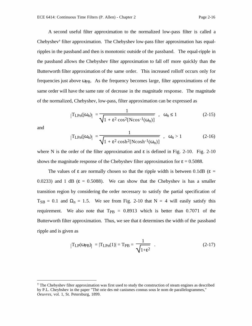
A second useful filter approximation to the normalized low-pass filter is called a

Chebyshev† filter approximation. The Chebyshev low-pass filter approximation has equal-

ripples in the passband and then is monotonic outside of the passband. The equal-ripple in

the passband allows the Chebyshev filter approximation to fall off more quickly than the

Butterworth filter approximation of the same order. This increased rolloff occurs only for

frequencies just above ωPB. As the frequency becomes large, filter approximations of the

same order will have the same rate of decrease in the magnitude response. The magnitude

of the normalized, Chebyshev, low-pass, filter approximation can be expressed as

| |TLPn(jωn) = 1

1 + ε2 cos2[Ncos-1(ωn)] , ωn ≤ 1 (2-15)

and

| |TLPn(jωn) = 1

1 + ε2 cosh2[Ncosh-1(ωn)] , ωn > 1 (2-16)

where N is the order of the filter approximation and ε is defined in Fig. 2-10. Fig. 2-10

shows the magnitude response of the Chebyshev filter approximation for ε = 0.5088.

The values of ε are normally chosen so that the ripple width is between 0.1dB (ε =

0.0233) and 1 dB (ε = 0.5088). We can show that the Chebyshev is has a smaller

transition region by considering the order necessary to satisfy the partial specification of

TSB = 0.1 and Ωn = 1.5. We see from Fig. 2-10 that N = 4 will easily satisfy this

requirement. We also note that TPB = 0.8913 which is better than 0.7071 of the

Butterworth filter approximation. Thus, we see that ε determines the width of the passband

ripple and is given as

| |TLP(ωPB) = |TLPn(1)| = TPB = 1

1+ε2 . (2-17)

† The Chebyshev filter approximation was first used to study the construction of steam engines as describedby P.L. Cheybshev in the paper "The orie des me canismes connus sous le nom de parallelogrammes,"Oeuvres, vol. 1, St. Petersburg, 1899.


0

0.2

0.4

0.6

0.8

1

0 0.5 1 1.5 2 2.5 3

TLPn(jωn)

A

N=5

N=2

N=4

N=3

1

1+ε2


Figure 2-10 - Magnitude response of a normalized Chebyshev low-pass filter

approximation for various orders of N and for ε = 0.5088.

The magnitude of the Chebyshev filter approximation at ωSB can be expressed from Eq. (2-

16) as

TLPn

ωSB

ωPB = |TLPn(Ωn)| = TSB =

1

1 + ε2 cosh2[Ncosh-1(Ωn)] . (2-18)

If the specifications are in terms of decibels, then Eq. (2-19) is more convenient in the form

20 log10(TSB) = TSB (dB) = -10 log10[ ]1 + ε2 cosh2[Ncosh-1(Ωn)] . (2-19)

Example 2-4 - Determining the Order of A Chebyshev Filter Approximaton

Repeat Ex. 2-2 for the Chebyshev filter approximation.

Solution

In Ex. 2-2, ε = 1 which means the ripple width is 3 dB or TPB = 0.707. Now we

substitute ε = 1 into Eq. (2-19) and find the value of N which satisfies TSB = - 20dB. For

N = 2, we get TSB = - 11.22 dB. For N =3, we get TSB = -19.14 dB. Finally, for N = 4,

we get TSB = -27.43 dB. Thus N = 4 must be used although N = 3 almost satisfies the

specifications.

The normalized pole locations, pkn, of the low-pass, normalized Chebyshev filter

approximation can be found from the following formula


pkn = σkn + jωkn = - sin

(2k-1)π

2N sinh

1

N sinh-11

ε + j cos

(2k-1)π

2N cosh

1

N sinh-11

ε

,

k = 1, 2, 3, ···, N . (2-20)

To illustrate this formula, the poles for a fifth-order, normalized, Chebyshev filter have

been evaluated are are given in Table 2-3 for the case where TPB = -1dB. It can be shown

that these poles lie on an ellipse centered about the origin of the complex frequency plane.

The pole locations for Table 2-3 are illustrated on Fig. 2-11.

k σkn = - sin

(2k-1)π

2N sinh

1

N sinh-11

ε ωkn = cos

(2k-1)π

2N cosh

1

N sinh-11

ε

1 -0.0895 rps 0.9901 rps

2 -0.2342 rps 0.6119 rps

3 -0.2895 rps 0.0000 rps

4 -0.2342 rps -0.6119 rps

5 -0.0895 rps -0.9901 rps

Table 2-3 - Normalized pole locations for a fifth-order, Chebyshev filter approximation for

ε = 0.5088.

jωn

σn1

j1

-1

-0.2342 -0.0895

j0.9901

j0.6119

-j0.6119

-j0.9901

-0.2895

UnitCircle

Ellipse on which poles lie

p1n

p2n

p3n

p4n

p5n

Figure 2-11 - Location of the normalized poles for a fifth-order, normalized Chebyschev

filter approximation for ε = 0.5088.


The normalized transfer function of the Chebyshev filter approximation can be written

as the product of second-order terms and one, first-order term if the order is odd. For the

fifth-order, Chebysheve filter approximation, the filter transfer function is written as

TLPn(sn) =

p3n

sn+p3n

p1np5n

(sn+p1n)(sn+p5n)

p2np4n

(sn+p2n)(sn+p4n) (2-21)

where we have grouped the complex-conjugate poles into second-order terms. Substituting

the values of Table 2-3 into Eq. (2-21) gives

TLPn(sn) = T1(sn)T2(sn)T3(sn) =

0.2895

sn+0.2895

0.9883

s2n+0.1789sn+0.9883

0.4239

s2n+0.4684sn+0.4239

. (2-22)

As before, each product does not necessarily have the characteristic of a Chebychev filter.

However, when all the products are multiplied together, the result is a Chebyschev filter

approximation.

The design procedure for designing a cascaded, Chebyshev filter approximation

using active filters is stated as follows:


the Chebyshev filter approximation using Eq. (2-18) or Eq. (2-19).

2.) From Eq. (2-20) find the normalized poles of the approximation.

3.) Group the complex-conjugate poles into second-order realizations. For odd-

order realizations there will be one first-order term of the form 1/(sn+1).

4.) Realize each of the second-order terms using the active filters of Sec. 1. Realize

the first-order section (if any) by the first-order low-pass circuits of Sec. 4.2.

5.) Cascade the realizations in the order from input to output of the lowest-Q stage

first (first-order stages generally should be first).


if desired.

The following example will illustrate the application of this design procedure.


Example 2-5 - Design of a Fifth-Order, Low-Pass Chebyshev Filter

Design a cascade, active filter realization for a Chebyshev filter approximation to the

filter specifications of APB = 1dB, ASB = 45 dB, fPB = 1 kHz, and fSB = 2 kHz. Give a

schematic for the realization using the negative feedback, second-order, low-pass active

filter of Fig. 1-14 and any first-order state that may be necessary. Show all values of the

components.

Solution

First we must convert the specifications to TPB = - 1dB, TSB = -45dB, and Ωn =

fSB/fPB = 2.0. TPB = -1 dB means ε = 0.5088. Trying different values of N in Eq. (2-20)

shows that for N = 5 that TSB = -45.3 dB. Thus, a fifth-order Chebyshev approximation

barely satisfies the requirement. Again, we might be smart to go to a sixth-order realization

to achieve a margin of safety but we shall stay with N = 5 for this example. N = 5 allows

us to take advantage of the previous results given above. Let us do the design stage-by-

stage.

Stage 1: Stage 1 is simply a first-order stage. Let us use Fig. 4.2-6c and choose

R11 = R21 = 1Ω. Therefore, from Eq. (4.2-17) we get C21 = 1

0.2895R21 = 3.454 F

where the second subscript stands for the stage number.


T2(sn) = 0.9883

s2n+0.1789sn+0.9883

.

From Eq. (1-3) we see that ωo = 0.9883 = 0.9941 rps and Q = Q2 = 0.9883

0.1789 =

5.557. Using the design equations of Eqs. (1-41) through (1-45) give C52 = 1 F ,

C42 = 4(5.557)2(1+1)C = 247.04 F, R12 = 1

(2)(1)(0.9941)(5.557)(1) = 0.09051 Ω,

R22 = 1

(2)(0.9941)(5.557)(1) = 0.09051 Ω, and R32 = 1

(2)(0.9941)(5.557)(1+1) =

0.04525 Ω.



T3(sn) = 0.4239

s2n+0.4684sn+0.4239

.

From Eq. (1-3) we see that ωo = 0.4239 = 0.6522 rps and Q3 = 0.4239

0.4684 =

1.390. Using the design equations of Eqs. (1-41) through (1-45) give C53 = 1 F ,

C43 = 4(1.390)2(1+1)C = 15.457 F, R13 = 1

(2)(1)(0.6522)(1.390)(1) = 0.5515 Ω,

R23 = 1

(2)(0.6522)(1.390)(1) = 0.5515 Ω, and R33 = 1

(2)(0.6522)(1.390)(1+1) =

0.2758 Ω.

Next, we frequency denormalize the filter realization by ωPB = 2πx103. At the same

time we will impedance denormalize by 105 (arbitrarily chosen). The resulting values are

shown on the realization of Fig. 2-12 and are achieved using the bottom row of Table 2-1.

Note, that we have placed stage 1 first, stage 3 second, and stage 2 last. This filter

realization will meet the specifications given and will permit maximum signal amplitude.

Figure 2-12 - A denormalized, fifth-order, active filter realization of a low-pass, Cheby-

shev filter approximation.

In comparing the results of Examples 2-3 and 2-5, we see that the realizations are

identical and it is the value of the components which distinguishes the Butterworth

approximation from the Chebyshev approximation. However, we should note that for the

same ωPB and ωSB, the Chebyshev approximation has a 1dB passband ripple compared to

a 3dB passband "ripple" for the Butterworth approximation. More importantly, the

stopband attenuation of the Chebyshev approximation is greater than 45 dB as compared to

Vin(s)

Stage 1

R11 =100kΩ

=100kΩR21 C21=5.50nF

Vo1 Vout(Vo2

Stage 2

C52 =1.59nF

C42=393nF

9.05kΩR12=

9.05kΩR22=

4.52kΩR32=

Stage 3

27.6kΩR33=

55.2kΩR23=

55.2kΩR13=

C43=24.6nF

C53=1.59nF


30 dB for the Butterworth. In fact, we could easily satisfy the requirements of Ex. 2-3

with a fourth-order Chebyshev approximation which would eliminate stage 1 of Fig. 2-12

(obviously, the components of stages 3 and 2 will change values).

High-Pass Active Filters

One of the useful principles of active filter design is that all design is based on the

normalized, low-pass filter approximation. Therefore, all we have to do is to transform the

normalized, low-pass filter design to a high-pass, bandpass, or bandstop design. If we let

sln be the normalized, low-pass frequency variable, the normalized, low-pass to

normalized, high-pass transformation is defined as

sln = 1

shn (2-23)

where shn is the normalized, high-pass frequency variable (normally the subscripts h and l

are not used when the meaning is understood). We have seen from the previous work that

a general form of the normalized, low-pass transfer function is

TLPn(sln) = p1lnp2lnp3ln···pNln

(sln+p1ln)(sln+p2ln)(sln+p3ln)···(sln+pNln) (2-24)

where pkln is the kth normalized, low-pass pole. If we apply the normalized, low-pass to

high-pass transformation to Eq. (2-24) we get

THPn(shn) = p1lnp2lnp3ln···pNln

1

shn +p1ln

1

shn +p2ln

1

shn +p3ln ···

1

shn +pNln

= s

Nhn

shn+

1p1ln

shn+

1p2ln

shn+

1p3ln

···

shn+

1pNln

= s

Nhn

( )shn+p1hn ( )shn+p2hn ( )shn+p3hn ···( )shn+pNhn (2-25)

where pkhn is the kth normalized high-pass pole.


We see that the normalized, low-pass to high-pass transformation inverts the pole

locations and causes all of the zeros to appear at the origin of the complex frequency plane.

Therefore, the design procedure is essentially the same as for the normalized, low-pass

filters except the poles are inverted and we associate with each pole a zero at the origin.

The order of the high-pass filter is determined by translating its specifications to an

equivalent low-pass filter. The general cascade design procedure for a high-pass filter is as

follows:

1.) Start with the high-pass specification in the form of Fig. 2-3b (or the equivalent

in terms of attenuation). Normalize the frequency by dividing by ωPB. Therefore,

the normalized passband frequency is 1 rps and the normalized bandstop frequency is

1Ωn

= Ωhn = ωSB

ωPB . (2-26)

Note that Ωhn will always be less than unity.


the filter approximation using the proper equations for the selected approximation.

3.) Find the normalized, low-pass poles of the approximation.

4.) Invert the normalized, low-pass poles (pkln) to get the normalized, high-pass

filter poles (pkhn).

5.) Group the complex-conjugate poles of the normalized, high-pass filter into

second-order realizations including 2 zeros at the origin. For odd-order realizations

there will be one first-order high-pass product.

6.) Realize each of the second-order terms using the high-pass, first- or second-order

active filters of Chapter 1.

7.) Cascade the realizations in the order from input to output of the lowest pole-Q

stage first (first-order stages generally should be first).

8.) Denormalize to the desired passband frequency and denormalize the impedances.



Example 2-6 - Design of a Butterworth, High-Pass Filter

Design a high-pass filter having a -3dB ripple bandwidth above 1 kHz and a gain of

less than -35 dB below 500 Hz using the Butterworth approximation. Use the positive

feedback active filter realization and give a complete circuit and all component values.

What is the value of the filter gain as frequency approaches infinity?

Solution

From the specification, we know that TPB = -3 dB and TSB = -35 dB. Eq. (2-26)

gives us an Ωn = 2 (Ωhn = 0.5). ε = 1 because TPB = -3 dB. Therefore, we use Eq. (2-

11) to find that N = 6 will give TSB = -36.12 dB which is the lowest, integer value of N

which meets the specifications.

Next, we evaluate the normalized, low-pass poles from Eq. (2-12) as

p1ln, p6ln = -0.2588 ± j 0.9659

p2ln, p5ln = -0.7071 ± j 0.7071and

p3ln, p4ln = -0.9659 ± j 0.2588

where the first subscript on the poles corresponds to k in Eq. (2-12). Inverting the

normalized, low-pass poles gives the normalized, high-pass poles which are

p1hn, p6hn = -0.2588 -+ j 0.9659

p2hn, p5hn = -0.7071 -+ j 0.7071and

p3hn, p4hn = -0.9659 -+ j 0.2588 .

We note the inversion of the Butterworth poles simply changes the sign of the imaginary

part of the pole.

The next step is to group the poles in second-order products, since there are no first-

order products. This result gives the following normalized, high-pass transfer function.

THPn(shn) = T1(shn)T2(shn)T3(shn)

=

s

2hn

(shn+p1hn)(shn+p6hn)

s

2hn


s

2hn



=

s

2hn

s2hn+0.5176shn+1

s

2hn

s2hn+1.4141shn+1

s

2hn

s2hn+1.9318shn+1

.

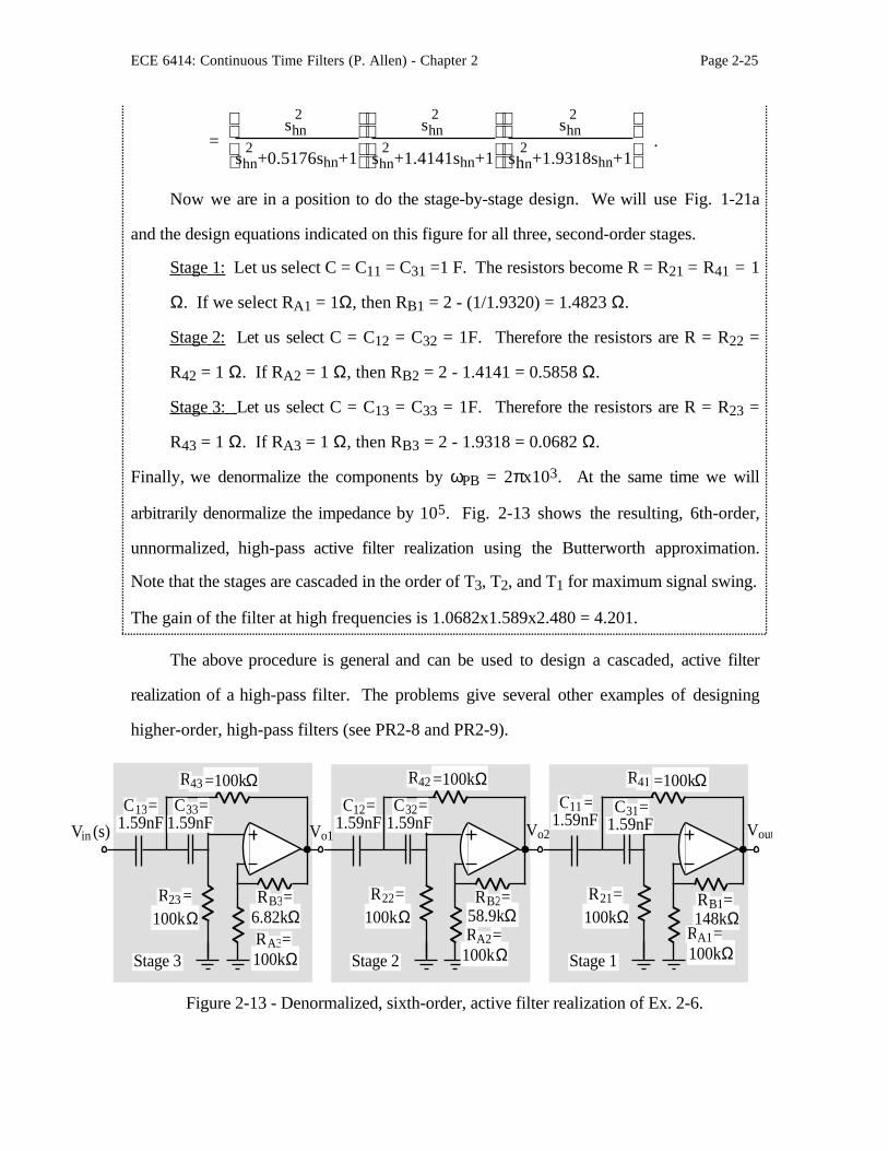
Now we are in a position to do the stage-by-stage design. We will use Fig. 1-21a

and the design equations indicated on this figure for all three, second-order stages.

Stage 1: Let us select C = C11 = C31 =1 F. The resistors become R = R21 = R41 = 1

Ω. If we select RA1 = 1Ω, then RB1 = 2 - (1/1.9320) = 1.4823 Ω.

Stage 2: Let us select C = C12 = C32 = 1F. Therefore the resistors are R = R22 =

R42 = 1 Ω. If RA2 = 1 Ω, then RB2 = 2 - 1.4141 = 0.5858 Ω.

Stage 3: Let us select C = C13 = C33 = 1F. Therefore the resistors are R = R23 =

R43 = 1 Ω. If RA3 = 1 Ω, then RB3 = 2 - 1.9318 = 0.0682 Ω.

Finally, we denormalize the components by ωPB = 2πx103. At the same time we will

arbitrarily denormalize the impedance by 105. Fig. 2-13 shows the resulting, 6th-order,

unnormalized, high-pass active filter realization using the Butterworth approximation.

Note that the stages are cascaded in the order of T3, T2, and T1 for maximum signal swing.

The gain of the filter at high frequencies is 1.0682x1.589x2.480 = 4.201.

The above procedure is general and can be used to design a cascaded, active filter

realization of a high-pass filter. The problems give several other examples of designing

higher-order, high-pass filters (see PR2-8 and PR2-9).

Figure 2-13 - Denormalized, sixth-order, active filter realization of Ex. 2-6.

Vin (s)

C11 =1.59nF

R41 =100kΩ

R21=100kΩ 148kΩ

RB1=

C31=1.59nF

100kΩRA1=

Stage 1

Vo2

Stage 2

58.9kΩRB2=

100kΩRA2=

R22=100kΩ

C12=1.59nF

C32=1.59nF

R42 =100kΩ

Stage 3

R43 =100kΩ

R23 =100kΩ

100kΩRA3=

6.82kΩRB3=

C13=1.59nF

C33=1.59nF Vo1 Vout


Bandpass Active Filters

We can continue to use our knowledge of low-pass filters to develop the other types

of filter responses indicated in Fig. 2-3. We will now develop bandpass filters which are

based on the normalized, low-pass filter. First, we define the width of the passband and

the width of the stopband of the bandpass filter as

BW = ωBP2 - ωPB1 (2-27)

and

SW = ωSB2 - ωSB1 , (2-28)

respectively. Our study here only pertains to a certain category of bandpass filters. This

category is one where the passband and stopband are geometrically centered about a

frequency, ωr, which is called the geometric center frequency of the bandpass filter. The

geometric center frequency of the bandpass filter is defined as

ωr = ωPB1ωPB2 = ωSB2ωSB1 . (2-29)

The geometrically centered bandpass filter can be developed from the normalized low-

pass filter by the use of a frequency transformation. If sb is the bandpass complex

frequency variable, then we define a normalized low-pass to unnormalized bandpass

transformation as

sln = 1

BW

sb

2 + ω r2

sb =

1BW

sb + ω r

2

sb . (2-30)

A normalized low-pass to normalized bandpass transformation is achieved by dividing the

bandpass variable, sb, by the geometric center frequency, ωr, to get

sln =

ωr

BW

sb

ωr +

1

(sb/ωr) =

ωr

BW

sbn + 1

sbn (2-31)

where

sbn = sb

ωr . (2-32)


We can multiply Eq. (2-31) by BW/ωr and define yet a further normalization of the low-

pass, complex frequency variable as

sln' =

BW

ωr sln = Ωbsln = Ωb

sl

ωPB =

sbn + 1

sbn (2-33)

where Ωb is a bandpass normalization of the low-pass frequency variable given as

Ωb = BW

ωr . (2-34)

We will call the normalization of Eq. (2-33) a bandpass normalization of the low-pass

complex frequency variable.

In order to be able to use this transformation, we need to solve for sbn in terms of sln'

. From Eq. (2-33) we get the following quadratic equation.

s2bn - sln

' sbn + 1 = 0 . (2-35)

Solving for sbn from Eq. (2-34) gives

sbn =

sln

'

2 ±

sln

'

22

- 1 . (2-36)

Figure 2-14 shows how transformation of Eq. (2-30) is used to create an unnormalized

bandpass filter from an unnormalized low-pass filter. We must remember that the low-pass

filter magnitude includes negative frequencies as indicated by the area enclosed by dashed

lines to the left of the vertical axis of Fig. 2-14a. The low-pass filter has been amplitude

normalized so that the passband gain is unity. Fig. 2-14b shows the normalization of the

frequency by ωPBl. Next, the low-pass to bandpass transformation of Eq. (2-31) is

applied to get the normalized, band-pass magnitude in Fig. 2-14c. Finally, the bandpass

filter is frequency denormalized to get the frequency unnormalized bandpass magnitude

response of Fig. 2-14d. The stopbands of the bandpass filter were not included for

purposes of simplicity but can be developed in the same manner.


(a.) (b.)

0 ωbn (rps)

1

00

TPBn(jωb)

ωr-ωr

BW BW

ωb (rps)

(c.)(d.)

Bandpass Normalization

Normalized low-pass to normalized bandpass

transformation

BandpassDenormalization

1

00-1 1

TLPn(jωln)

ωln (rps)ωrωPB

1

00

1Ωb-Ωb

TLPn(jωln' )

ωln' (rps)

sln'

2 ±

sln'

2

2

- 1

↓sbn

1

0

TBPn(jωbn)

ΩbΩb

1-1

sb ← Ωbsbn = BWωr

sbn

Ωbsln = BWωr

sln → sln'

Figure 2-14 - Illustration of the development of a bandpass filter from a low-pass filter. (a.)

Ideal normalized, low-pass filter. (b.) Normalization of (a.) for bandpass transformation.

(c.) Application of low-pass to bandpass transformation. (d.) Denormalized bandpass

filter.

Once the normalized, low-pass poles, p ' kln , are known, then the normalized

bandpass poles can be found from

pkbn = p ' k l n2 ±

p ' k l n

22

- 1 . (2-37)

which is written from Eq. (2-36). For each pole of the low-pass filter, two poles result for

the bandpass filter. Consequently, the order of complexity based on poles is 2N for the

bandpass filter. If the low-pass pole is on the negative real axis, the two bandpass poles

are complex conjugates. However, if the low-pass pole is complex, two bandpass poles

result from this pole and two bandpass poles result from its conjugate. Fig. 2-15 shows

how the complex conjugate low-pass poles contribute to a pair of complex conjugate


bandpass poles. p* is the designation for the conjugate of p. This figure shows that both

poles of the complex conjugate pair must be transformed in order to identify the resulting

two pairs of complex conjugate poles.

pjln'

pkln'

= pjln' *

pkbn*

pjbn*

pjbn

pkbn

jωln'

σln' σbn

jωbn

Low-pass PolesNormalized by ωPBωr

BWNormalized

Bandpass Poles

Figure 2-15 - Illustration of how the normalized, low-pass, complex conjugate poles are

transformed into two normalized, bandpass, complex conjugate poles.

It can also be shown that the low-pass to bandpass transformation takes each zero at

infinity and transforms to a zero at the origin and a zero at infinity. After the low-pass to

bandpass transformation is applied to N-th order low-pass filter, there will be N complex

conjugate poles, N zeros at the origin, and N zeros at infinity. We can group the poles and

zeros into second-order products having the following form

Tk(sbn) = Kksbn

(sbn + pkbn)(sbn + pjbn* )

= Kksbn

(sbn+σkbn+jωkbn)(sbn+σkbn-jωkbn)

= Kksbn

sbn2

+(2σkbn)sbn+(σbn2

+ωkbn2

) =

Tk(ωkon)

ωkon

Qksbn

sbn2

+

ωkon

Qksbn + ωkon

2 (2-38)

where j and k corresponds to the jth and kth low-pass poles which are a complex conjugate

pair, Kk is a gain constant, and

ωkon = σkbn2

+ωkbn2

(2-39)


and

Qk = σbn

2+ωkbn

2

2σbn . (2-40)

Normally, the gain of Tk(ωkon) is unity.

The order of the bandpass filter is determined by translating its specifications to an

equivalent low-pass filter. The ratio of the stop bandwidth to the pass bandwidth for the

bandpass filter is defined as

Ωn = SWBW =

ωSB2 - ωSB1

ωBP2 - ωPB1 . (2-41)

The general cascade design procedure for a bandpass filter follows:

1.) Start with the bandpass specification in the form of Fig. 2-3c (or the equivalent in

terms of attenuation). Normalize the frequency by dividing by ωr . Therefore, the

normalized geometric center frequency is 1 rps and the normalized bandwidth Ωb.


the normalized, low-pass filter approximation using the proper equations for the

selected approximation.

3.) Find the normalized, low-pass poles of the approximation.

4.) Frequency scale (normalize) the normalized, low-pass poles by Ωb = (BW/ωr).

5.) Find the normalized poles of the bandpass filter by inserting each normalized

low-pass pole into Eq. (2-37).

6.) Group the complex conjugate poles in to the form of Eq. (2-38).

7.) Realize each complex conjugate pole pair by a second-order, bandpass active

filter.

8.) Cascade the realizations in the order from input to output of the lowest pole-Q

stage first.


if desired using Eq. (2-32) and Table 2-1.



Example 2-7 - Design of a Butterworth, BandPass Filter

Design a bandpass, Butterworth filter having a -3dB ripple bandwidth of 200 Hz

geometrically centered at 1 kHz and a stopband of 1 kHz with an attenuation of 40 dB or

greater, geometrically centered at 1 kHz. Use the Tow-Thomas active filter realization and

give a complete circuit and all component values. The gain at 1 kHz is to be unity.

Solution

From the specifications, we know that TPB = -3 dB and TSB = -40 dB. Eq. (2-39)

gives a value of Ωn = 1000/200 = 5. ε = 1 because TPB = -3 dB. Therefore, we use Eq.

(2-11) to find that N = 3 will give TSB = -41.94 dB which is the lowest, integer value of N

which meets the specifications.

Next, we evaluate the normalized, low-pass poles from Eq. (2-12) as

p1ln, p3ln = -0.5000 ± j0.8660and

p2ln = -1.0000 .

where the first subscript on the poles corresponds to k in Eq. (2-12). Normalizing these

poles by the bandpass normalization of Ωb = 200/1000 = 0.2 gives

p ' 1ln , p ' 3ln = -0.1000 ± j 0.1732

andp ' 2ln = -0.2000 .

Each one of the p ' kln will contribute a second-order term of the form given in Eq. (2-

37). The normalized bandpass poles are found by using Eq. (2-36) which results in 6

poles given as follows. For p ' 1ln = -0.1000 + j0.1732 we get

p1bn, p2bn = -0.0543 + j1.0891, -0.0457 - j0.9159.

For p ' 3ln = -0.1000 - j0.1732 we get

p3bn, p4bn = -0.0457 + j0.9159, -0.543 - j 1.0891.

For p ' 2ln = -0.2000 we get

p5bn, p6bn = -0.1000 ± j 0.9950.


Fig. 2-16 shows the normalized low-pass pole locations, pkln, the bandpass normalized,

low-pass pole locations, pkln' , and the normalized bandpass poles, pkbn. Note that the

bandpass poles have very high pole-Qs if BW < ωr.

p1ln

p2ln

p3ln

p3ln'

p2ln'p1ln

'

j1

-j1

-1σln

'

jωln'

(b.)(a.)

-1

j1

-j1

-0.5000

j0.8660

-j0.8660

jωln

σln

p1ln

p2ln

p3ln

σbn

p1bn

p2bn

p3bn

p4bn

p5bn

p6bn

jωbn

j1

-1

-j1

(c.)

3 zerosat ±j∞

Figure 2-16 - Pole locations for Ex. 2-7. (a.) Normalized low-pass poles. (b.) Bandpass

normalized low-pass poles. (c.) Normalized bandpass poles.

Grouping the complex conjugate bandpass poles gives the following second-order

transfer functions.

T1(sbn) = K1sbn

(s+p1bn)(s+p4bn) =

K1sbn(sbn+0.0543+j1.0891)(sbn+0.0543-j1.0891)

=

1.0904

10.0410 sbn

sbn2

+

1.0904

10.0410 sbn+1.09042 .

T2(sbn) = K2sbn

(s+p2bn)(s+p3bn) =

K2sbn(sbn+0.0457+j0.9159)(sbn+0.0457-j0.9159)

=

0.9170

10.0333 sbn

sbn2

+

0.9170

10.0333 sbn+0.91592

.

and

T3(sbn) = K3sbn

(s+p5bn)(s+p6bn) = K3sbn

(sbn+0.1000+j0.9950)(sbn+0.1000-j0.9950)


=

1.0000

5.0000 sbn

sbn2

+

1.0000

5.0000 sbn+1.00002 .

Now we are in a position to do the stage-by-stage design. We will use Fig. 1-22 and

the design equations of Eqs. (1-60), (1-61), and (1-73) for all three, second-order stages.

Stage 1: Let us select C = C11 = C21 =1 F. From Eq. (1-60), the resistors R21 and

R31 are designed as R = R21 = R31 = 1/(ω1onC) = 1/(1.09043)(1) = 0.9171 Ω. Eq.

(1-61) gives R41 = QR = (10.0410)(0.9171) = 9.2083 Ω. Finally, Eq. (1-73) gives

R11 = R41 = 9.2083 Ω.


R32 are designed as R = R22 = R32 = 1/(ω2onC) = 1/(0.9159)(1) = 1.0918 Ω. Eq.

(1-61) gives R42 = QR = (10.0333)(1.0918) = 10.9546 Ω. Finally, Eq. (1-73) gives

R12 = R42 = 10.9546 Ω.


R33 are designed as R = R23 = R33 = 1/(ω3onC) = 1/(1)(1) = 1.0000 Ω. Eq. (1-61)

gives R41 = QR = (5.0000)(1.0000) = 5.0000 Ω. Finally, Eq. (1-73) gives R13 =

R43 = 5.0000 Ω.

Finally, we denormalize the components by ωr = 2πx103. At the same time we will

arbitrarily denormalize the impedance by 104. Fig. 2-17 shows the resulting, sixth-order,

unnormalized, bandpass active filter realization using the Butterworth approximation. Note

that the stages are cascaded in the order of T3, T2, and T1 for maximum signal swing.

The bandpass design procedure illustrated in Ex. 2-7 is general and can be used to

design a cascaded, active filter realization of a bandpass filter whose bandwidth is

geometrically centered around a frequency, ωr. The problems give several other examples

of designing higher-order, high-pass filters (see PR2-11 and PR2-12).


Vin(s)

A13 A23

A33

10 kΩ

Stage 3

A12 A22

A32

10 kΩ

10 kΩ

Stage 2

A11 A21

A31

R31 = 9.171 kΩ

R41 = 92.08 kΩ

10 kΩ

10 kΩ

C21 = 15.91 nF

C11 = 15.91 nF

R21 = 9.171 kΩ

R11 = 92.08 kΩ

Stage 1

R12 = 109.55

kΩ

R42 =

109.5 kΩ R22 = 10.92

kΩ

R32 = 10.92kΩ C22 = 15.91 nF

C12 = 15.91 nF

C13 = 15.91 nF

C23 = 15.91 nFR33= 10kΩ

R13 =

kΩ

R23 = 10.00

kΩ

R43 = 50.00kΩ

Vout(s)

50.00

10 kΩ

10 kΩ

Figure 2-17 - Sixth-order, Butterworth filter realization for Ex. 2-7.

Active Filters with Finite Complex Conjugate Zeros

Some filter approximations which we have not studied use finite complex conjugate

zeros as well as complex conjugate poles. Typically, these zeros are on the jω axis

although they may be either in the left-half or right-half complex frequency plane. The

advantage of having complex conjugate zeros is that these zeros may be placed in the

stopband to make the attenuation of the filter approximation greater for a given transition

region. Fig. 2-18 shows an approximation called elliptic filter approximation. The elliptic

filter has equal ripple bands in both the passband and the stopband. The number of poles

must be equal to or greater than the number of zeros so that the magnitude of the low-pass

filter rolls off to zero as frequency approaches infinity.

jω axiszeros

0

0.2

0.4

0.6

0.8

1

0 0.5 1 1.5 2 2.5 3

TLPn(jωn)

A1

1+ε2


B

Figure 2-18 - Magnitude response of a fifth-order, elliptic filter approximation.


The elliptic filter approximation has the steepest possible roll off in the transition

region of any type of filter approximation. This steep roll off is due to the presence of

complex conjugate zeros on the jω axis just outside of the passband. The realization of

filters containing jω axis zeros is exactly the same as been previously demonstrated in this

section. The filter design starts from the normalized, low-pass structure which will contain

complex conjugate zeros. The realization uses the cascade of first- and second-order active

filters. However, this time, the active filters must be capable of realizing the complex

conjugate zeros. The biquad, second-order active filter discussed in the last section is

useful for this purpose. See the problems for further details on the design of filters with

complex conjugate zeros (see PA2-2 and PA2-3).

Summary

The emphasis of this section has been on the design of higher-order filters using the

cascade of first- and second-order active filter realizations. The normalized low-pass filter

approximation is the starting point of all filter designs. The normalized low-pass filter has

a passband from 0 to 1 rps. A filter is completely specified by four quantities: 1.)

passband region, 2.) ripple of the passband region, 3.) stopband region, and 4.) the ripple

of the stopband region. We use the word "ripple" even for those filter approximations

which are monotonic.

We have examined two popular filter approximations. They are the Butterworth and

the Chebyshev approximations. An approximation is a transfer function in the complex

frequency variable which will satisfy the filter specification. The order of the

approximation is a measure of the complexity of a realization. It is generally preferable to

keep the order as small as possible.

There are four types of filters that have been considered. These types are the low-

pass, high-pass, bandpass, and bandstop. The normalized low-pass filter is the starting

point for the design of these different types of filters. Frequency transformations are used

to take the low-pass filter approximation to the other types of filters. It is important to


remember if the frequency transformations are used for the bandpass filters (and bandstop

filters) that the filter passband and stopband must be geometrically related to a center

frequency, ωr.

The realization of higher-order filters discussed in this section uses the cascade of

first- and second-order active filters. The design of each cascaded active filter uses a set of

design equations which permit the designer to find the value of the components of the filter

in terms of the first- or second-order transfer function. The design of these active filters is

usually done for the normalized approximation and then a frequency denormalization and

an impedance denormalization (which is generally arbitrary) is used to achieve the actual

filter specifications and to get practical component values.

A word of caution is in order concerning the filters that have been discussed in this

section. The design techniques introduced work well until the frequency of the filter begins

to become larger than about 10 kHz. At this point, the frequency response of the op amp

can no longer be ignored. Some of the realizations are more susceptible than others to the

influence of the op amp frequency response. There are methods which permit active filters

to be extended to 100 kHz and above but they are beyond the scope of this chapter. It has

been observed that the influence of the op amp frequency response on the filter

performance increases as the Q of the pole becomes higher.

2 - higher-order, cascaded, active...

Documents