MATRIX FUNCTIONS

ANDREAS FROMMER∗ AND VALERIA SIMONCINI†

1. Introduction. In this chapter, we give an overview on methods to computefunctions of a (usually square) matrix A with particular emphasis on the matrixexponential and the matrix sign function. We will distinguish between methods whichindeed compute the entire matrix function, i.e. they compute a matrix, and thosewhich compute the action of the matrix function on a vector. The latter task isparticularly important in the case where we have to deal with a very large (andpossibly sparse) matrix A or in situations, where A is not available as a matrix butjust as a function which returns Ax for any input vector x. Computing the action of amatrix function on a vector is a typical model reduction problem, since the resultingtechniques usually rely on approximations from small-dimensional subspaces.

This chapter is organized as follows: In section 2 we introduce the concept of amatrix function f(A) in detail, essentially following [37] and [27]. Section 3 gives anassessment of various general computational approaches for either obtaining the wholematrix f(A) or its action f(A)v on a vector v. Sections 4 and 5 then give much moredetails for two specific functions, the exponential and the sign functions, which, as wewill show, are particularly important in many areas like control theory, simulation ofphysical systems and other application fields involving the solution of certain ordinaryor partial differential equations. The applicability of matrix functions in general, andof the exponential and the sign functions in particular, is vast. However, we willlimit our discussion to characterizations and to application problems that are mostlyrelated to Model Order Reduction.

2. Matrix Functions. In this section we address the following general question:Given a function f : C → C, is there a canonical way to extend this function to squarematrices, i.e. to extend f to a mapping from C

n×n to Cn×n? If f is a polynomial p

of degree d, f(z) = p(z) =∑d

k=0 akzk, the canonical extension is certainly given by

p : Cn×n → C

n×n, p(A) =

d∑

k=0

akAk.

If f(z) can be expressed by a power series, f(z) =∑∞

k=0 akzk, a natural next step isto put

f(A) =

∞∑

k=0

akAk, (2.1)

but for (2.1) to make sense we must now discuss convergence issues. The main result isgiven in the following theorem, the proof of which gives us valuable further informationon matrix functions. Recall that the spectrum spec(A) is the set of all eigenvalues ofA.

∗Fachbereich Mathematik und Naturwissenschaften, Universitat Wuppertal, D-42097 Wuppertal,frommer@math.uni-wuppertal.de

†Dipartimento di Matematica, Universita di Bologna, Piazza di Porta S. Donato 5, I-40127Bologna, and CIRSA, Ravenna, Italy valeria@dm.unibo.it

1

Theorem 2.1. Assume that the power series f(z) =∑∞

k=0 akzk is convergentfor |z| < ρ with ρ > 0 and assume that spec(A) ⊂ z ∈ C : |z| < ρ. Then the series(2.1) converges.

Proof. Let T be the transformation matrix occuring in the Jordan decomposition

A = TJT−1, (2.2)

with

J =

Jm1(λ1) 0

. . .

0 Jm`(λ`)

=: diag(Jm1

(λ1), . . . , Jm`(λ`) ).

Here, λ1, . . . , λ` are the (not necessarily distinct) eigenvalues of A and mj is the sizeof the jth Jordan block associated with λj , i.e.

Jmj(λj) =

λj 1 0 · · · 0

0 λj 1. . .

......

. . .. . .

. . . 0...

. . .. . . 1

0 · · · · · · 0 λj

=: λjI + Smj∈ C

mj×mj ,

and∑`

j=1 mj = n. For each λj , the powers of Jmj(λj) are given by

Jm(λj)k =

k∑

ν=0

(k

ν

)λk−ν

j · Sνmj

.

Note that Sνmj

has zero entries everywhere except for the ν-th upper diagonal, whoseentries are equal to 1. In particular, Sν

mj= 0 for ν ≥ mj . Therefore,

f(Jmj(λj)) =

∞∑

k=0

ak

k∑

ν=0

(k

ν

)λk−ν

j · Sνmj

,

and for ν and j fixed we have

∞∑

k=0

ak

(k

ν

)λk−ν

j =∞∑

k=0

1

ν!· ak · (k · . . . · (k − ν + 1))λk−ν

j =1

ν!f (ν)(λj).

Note that the last equality holds in the sense of absolute convergence because λj

lies within the convergence disk of the series. This shows that the series f(Jmj(λj))

converges. Plugging these expressions into the series from (2.1) we obtain the valueof the original (now convergent) series,

f(A) = Tdiag (f(Jm1(λ1)), . . . , f(Jm`

(λ`)))) T−1

= Tdiag

(m1−1∑

ν=0

1

ν!f (ν)(λ1) · Sν

m1, . . . ,

m`−1∑

ν=0

1

ν!f (ν)(λ`) · Sν

m`

)T−1. (2.3)

2

It may happen that a function f cannot be expressed by a series converging in alarge enough disk. If f is sufficiently often differentiable at the eigenvalues of A, thenthe right-hand side of (2.3) is still defined. We make it the basis of our final definitionof a matrix function.

Definition 2.2. Let A ∈ Cn×n be a matrix with spec(A) = λ1, . . . , λ` and

Jordan normal form

J = T−1AT = diag(Jm1(λ1), . . . , Jm`

(λ`) ).

Assume that the function f : C → C is mj−1 times differentiable at λj for j = 1, . . . , `.Then the matrix function f(A) is defined as f(A) = Tf(J)T−1 where

f(J) = diag(f(Jm1(λ1)), . . . , f(Jm`

(λ`))) with f(Jmj(λj)) =

mj−1∑

ν=0

1

ν!f (ν)(λj) · Sν

mj.

This definition makes explicit use of the Jordan canonical form and of the asso-ciated transformation matrix T . Neither T nor J are unique, but it can be shown –as is already motivated by (2.1) – that f(A) as introduced in Definition 2.2 does notdepend on the particular choice of T or J .

As a first consequence of Definition 2.2 we note the following important property.Proposition 2.3. With the notation above, it holds f(A) = p(A), where p is the

polynomial of degree not greater than n − 1 which interpolates the eigenvalues λj ofA in the Hermite sense (i.e. f (ν)(λj) = p(ν)(λj) for all relevant ν’s and j’s).

The polynomial p in Proposition 2.3 will not only depend on f , but also on Aor, more precisely, on the minimal polynomial of A (of which the multiplicity of aneigenvalue λ determines the maximal block size mj for the Jordan blocks correspond-ing to this eigenvalue). When A is normal, T is an orthogonal matrix and all Jordanblocks have size one, i.e. we have

J = diag(λ1, . . . , λn).

So, in this particular case, we do not need any differentiability assumption on f .A further representation of f(A) can be derived in the case when f is analytic in

a simply connected region Ω containing spec(A). Let γ be a curve in Ω with windingnumber +1 w.r.t. a point z ∈ Ω. The Residue Theorem tells us

f (ν)(z)

ν!=

1

2πi

∮

γ

f(t)

(t − z)ν+1dt. (2.4)

Let Jmj(λj) be a Jordan block associated with λj and let z 6= λj . Then

(zI − Jmj)−1 = ((z − λj)I − Smj

)−1 =1

z − λj·

mj−1∑

ν=0

(1

z − λj· Smj

)ν

,

from which we get

1

2πi

∮

γ

f(z)(zI − Jmj)−1 =

mj−1∑

ν=0

1

2πi

∮

γ

f(z)

(z − λj)ν+1Sν

mjdt

=

mj−1∑

ν=0

f (ν)(λj)

ν!· Sν

mj,

3

the second line holding due to (2.4). Using this for each Jordan block in Definition 2.2and recombining terms we obtain the following integral representation of f(A),

f(A) =1

2πi

∮

γ

f(t)(tI − A)−1dt. (2.5)

3. Computational aspects. It is not necessarily a good idea to stick to oneof the definitions of matrix function given in the previous section when it comes tonumerically compute a matrix function f(A). In this section we will discuss such com-putational issues, describing several numerical approaches having their advantages indifferent situations, basically depending on spectral properties of A, on the dimensionand sparsity of A and on whether we really want to obtain the matrix f(A) ratherthan “just” its action f(A)v on a vector v.

3.1. Normal matrices. A matrix A ∈ Cn×n is said to be normal if it commutes

with its adjoint, AAH = AHA. Normal matrices may also be characterized as beingunitarily diagonalizable, i.e. we have the representation

A = QΛQH with Q−1 = QH , Λ = diag(λ1, . . . , λn), spec(A) = λ1, . . . , λn.

This representation is also the Jordan decomposition of A from (2.2), so that

f(A) = Qf(Λ)QH , f(Λ) = diag(f(λ1), . . . , f(λn)). (3.1)

Normal matrices have the very attractive property that their eigenvalues λi and thecorresponding invariant subspaces are well conditioned (see [16], for example), i.e.small changes in A yield only small changes in Λ and Q. Therefore, if we use anumerically (backward) stable algorithm to compute Λ and Q, like, for example,the standard Householder reduction to upper Hessenberg form followed by the QR-iteration, we may safely use the so computed Λ and Q to finally compute f(A) via(3.1). The computational cost of this approach is O(n3) due to the various matrix-matrix multiplications and to the cost for computing the eigendecomposition.

If A is not normal, its eigenvalues are not necessarily well conditioned, the con-dition number being related to ‖T‖2 · ‖T−1‖2 with T from the Jordan decomposition(2.2). It is also important to realize that the size of the Jordan blocks may widely varyunder infinitesimal perturbations in A. Therefore, if A is not normal, Definition 2.2does not provide a numerically stable means for computing f(A).

3.2. Quadrature rules. Assume that f is analytic in Ω and that γ and Ω areas in (2.5) so that we have

f(A) =1

2πi

∮

γ

f(t)(tI − A)−1dt.

We apply a quadrature rule with m nodes tj ∈ γ and weights ωj to the right-handside to get

1

2πi

∮

γ

f(t)

t − zdt =

m∑

j=1

ωjf(tj)

tj − z+ r.

This shows that we can approximate

f(A) ≈m∑

j=1

ωjf(tj) · (tjI − A)−1. (3.2)

4

For such quadrature rules, the approximation error r can be expressed or boundedusing higher derivatives of f . Actually, since we integrate over a closed curve, takingthe right nodes the quadrature error is usually much smaller than what one wouldexpect from quadrature formulas over finite (real) intervals, and the accuracy oftenincreases exponentially with the number of nodes, see [14],[15]. In principle, this canthen be used to obtain bounds on the approximation error in (3.2), but to do so weusually need some knowledge about the norms of T and T−1 in (2.2), as well as onthe size of the eigenvalues of A. See also section 3.6.

For specific functions, other integral representations may be used. For example,for z ∈ C, z not on the non-positive real line, we have (see [14])

log(z) =

∫ 1

0

(z − 1)[t(z − 1) + 1]−1dt,

so that using a quadrature rule for the interval [0, 1], we can use the approximation

log(A) ≈m∑

j=1

ωj · (A − I)[tj(A − I) + I]−1.

As another example, for z > 0 we can write

z−1/2 =2

π·∫ ∞

0

1

t2 + zdt,

and use a quadrature rule on [0,∞] to approximate A−1/2 when spec(A) ⊂ (0,∞].Similar approaches have been proposed for various other functions like the p-th

root or the sign function, see [6], [57], for example.Within this quadrature framework, the major computational cost will usually be

due to the inversion of several matrices. As is explained in [14], this cost can oftenbe reduced if we first compute a unitary reduction to upper Hessenberg form (whichcan be done in a numerically stable manner using Householder transformations), i.e.

A = QHQH , Q unitary , H zero below the first subdiagonal.

Then, for example,

(tjI − A)−1 = Q · (tjI − H)−1 · QH for all j,

with the inversion of the matrix tjI − H having cost O(n2) rather than O(n3).

3.3. Matrix iterations. Sometimes, it is convenient to regard f(z) as the solu-tion of a fixed point equation gz(f) = f with gz being contractive in a neighbourhoodof the fixed point f(z). The method of successive approximations

fk+1 = gz(fk) (3.3)

can then be turned into a corresponding matrix iteration

Fk+1 = gA(Fk). (3.4)

Approaches of this kind have, for example, been proposed for the matrix square root[31], [32], where Newton’s method

fk+1 =1

2·(

fk +z

fk

)(3.5)

5

to compute√

z results in the iteration

Fk+1 =1

2·(Fk + A · F−1

k

). (3.6)

Similar other iterations, not always necessarily derived from Newton’s method, havebeen proposed for the matrix p-th root [6] or for the matrix sign function [40]. Amajor catch with these approaches is that numerical stability of the matrix iteration(3.4) is not always guaranteed, even when the scalar iteration (3.3) is perfectly stable.Then, some quite subtle modifications, like e.g. the coupled two-term iteration for thesquare root analyzed in [31] must be used in order to achieve numerical stability. Theiteration (3.4) is usually also quite costly. For example, (3.6) requires the inversionof Fk at every step, so that each step has complexity O(n3). Therefore, for thesemethods to be efficient, convergence should be fast, at least superlinear.

3.4. Rational approximations. Polynomial approximations for a function foften require a quite high degree of the approximating polynomial in order to achievea reasonable quality of approximation. Rational approximations typically obtain thesame quality with substantially fewer degrees of freedom.

Assume that we have the rational approximation

f(z) ≈ Nµν(z)

Dµν(z),

where Nµν ,Dµν are polynomials of degree µ and ν, respectively. (The use of thetwo indices µ and ν in both polynomials may appear abusive at this point, but itwill be very convenient when discussing Pade approximations to the exponential insection 4.2). Then

f(A) ≈ Nµν(A) · (Dµν(A))−1

.

Assume that A is diagonalizable. If we know

∣∣∣∣f(z) − Nµν(z)

Dµν(z)

∣∣∣∣ ≤ ε for z ∈ spec(A),

we get

‖f(A) −Nµν(A) · (Dµν(A))−1 ‖2 ≤ ε · ‖T‖2 · ‖T−1‖2

which further simplifies when A is normal, since then T is unitary so that ‖T‖2 ·‖T−1‖2 = 1. Rational functions can be expressed as partial fraction expansions.Simplifying our discussion to the case of single poles, this means that we can expand

Nµν(z)

Dµν(z)= p(z) +

ν∑

j=1

ωj

z − τj,

with p(z) being a polynomial of degree µ − ν if µ ≥ ν and p ≡ 0 if µ < ν. Thisrepresentation is particularly useful if we are interested only in f(A)v for some vectorv, as we will discuss later in section 3.6. Note also that the quadrature rules from(3.2) immediately give a partial fraction expansion, so that the two approaches arevery closely related. For a recent investigation, see [65].

6

3.5. Krylov subspace approaches. When A has large dimension, the action off(A) on a vector v, namely f(A)v, may be effectively approximated by projecting theproblem onto a subspace of possibly much smaller dimension. The Krylov subspace

Kk(A, v) = spanv,Av, . . . , Ak−1v

has been extensively used to this purpose, due to its favourable computational andapproximation properties, see, e.g., van der Vorst [67], [68] for a discussion for generalf . Let Vk be a full column rank n × k matrix whose columns span Kk(A, v), andassume the following Arnoldi type recurrence holds for Vk,

AVk = Vk+1Hk+1,k = VkHk + hk+1,kvk+1eTk . (3.7)

An approximation to x = f(A)v may be obtained as

xk = Vkf(Hk)e1‖v‖. (3.8)

The procedure amounts to projecting the matrix onto the much smaller subspaceKk(A, v), by means of the representation matrix Hk and v = Vke1‖v‖. If Vk hasorthonormal columns then Hk = V T

k AVk. If in addition A is Hermitian, the iteration(3.7) reduces to the Lanczos three-term recurrence, in which case Hk is tridiagonaland Hermitian.

The functional evaluation is carried out within this reduced space, and the ob-tained solution is expanded back to the original large space. Assume now that k = niterations can be carried out, so that the square matrix Vn is orthogonal. Then (3.7)gives AVn = VnHn and thus A = VnHnV T

n . Using this relation, for k < n, the ap-proximation in Kk(A, v) may be viewed as a problem order reduction to the first kcolumns of Vn and corresponding portion of Hn as

x = f(A)v = Vnf(Hn)V Tn v ≈ Vkf(Hk)V T

k v.

For k small compared to n, the quality of the approximation strongly depends on thespectral properties of A and on the capability of Kk(A, v) to capture them. A firstcharacterization in this sense is given by the following result, which can be deducedfrom Proposition 2.3 applied to the matrix Hk and the fact that p(A)v = Vkp(Hk)vfor all polyomials of degree less than or equal to k − 1; see [60, Proposition 6.3]. Thisis a generalization of [59, Theorem 3.3].

Proposition 3.1. Let the columns of Vk, with V Tk Vk = Ik span Kk(A, v) and

let Hk = V Tk AVk. Then, the approximation Vkf(Hk)e1‖v‖ represents a polynomial

approximation p(A)v to f(A)v, in which the polynomial p of degree k− 1 interpolatesthe function f in the Hermite sense on the set of eigenvalues of Hk.

Other polynomial approximations have been explored, see, e.g., [18]; approachesthat interpolate over different sets have been proposed for the exponential function[52]. Note that the projection nature of the approach allows to derive estimates for‖f(A)‖ as ‖f(A)‖ ≈ ‖f(Hk)‖ which may be accurate even for small k when A isHermitian.

All these results assume exact precision arithmetic. We refer to [17] for an analysisof finite precision computation of matrix functions with Krylov subspace methodswhen A is Hermitian.

It should be mentioned that the projection onto a Krylov subspace does notrequire A to be stored explicitly, but it only necessitates a function that given v,

7

returns the action of A, namely y = Av. This operational feature is of paramountimportance in applications where, for instance, A is the (dense) product or othercombination of sparse matrices, so that the operation y = Av may be carried out bya careful application of the given matrix combination.

Another practical aspect concerns the situation where k, the dimension of theKrylov subspace, becomes large. Computing f(Hk) with one of the methods presentedin the previous sections can then become non-negligible. Moreover, we may run intomemory problems, since approximating f(A)v via (3.8) requires the whole matrix Vk

to be stored. This is needed even when, for istance, A is Hermitian, in which case(3.7) is the Lanczos recurrence and Hk is tridiagonal. In such a situation, however, wecan resort to a “two–pass” procedure which crucially reduces the amount of memoryneeded: In the first pass, we run the short-term recurrence Lanczos process. Here,older columns from Vk can be discarded, yet the whole (tridiagonal) matrix Hk canbe built column by column. Once f(Hk) has been generated, we compute yk =f(Hk)e1 · ‖v‖. Then we run the short-term recurrence modification of the Lanczosprocess once again to recompute the columns of Vk and use them one at a time tosum up Vkf(Hk)e1 = Vkyk. Of course, this two-stage approach essentially doublesthe computational work.

For a general matrix A the Arnoldi process cannot be turned into a short-termrecurrence, so one must search for alternatives in the case that k gets too large.Recently, Eiermann and Ernst [20] have developed an interesting scheme that allowsto restart Krylov subspace methods for computing f(A)v, in the same flavour aswith linear system solvers; in fact, the two approaches are tightly related; see [46].Having computed a not yet sufficiently good approximation xk via (3.8), the idea is tostart again a Krylov subspace approximation based on the error xk − f(A)v which isexpressed as a new matrix function of A. The algorithmic formulation is non-trivial,particularly since special care has to be taken with regard to numerical stability, see[20].

Other alternatives include acceleration procedures, that aim at improving theconvergence rate of the approximation as the Krylov subspace dimension increases.Promising approaches have been recently proposed in the Hermitian case by Druskinand Knizhnerman [19], by Moret and Novati [51] and by Hochbruck and van denEshof [36].

3.6. Krylov subspaces and rational approximations. As a last contributionto this section, let us turn back to rational approximations for f which we assume tobe given in the form of a partial fraction expansion (no multiple poles for simplicity)

f(z) ≈ p(z) +

ν∑

j=1

ωj

z − τj.

Then f(A)v can be approximated as

f(A)v ≈ p(A)v +

ν∑

j=1

ωj(A − τjI)−1v. (3.9)

Since evaluating p(A)v is straightforward, let us assume p ≡ 0 in the sequel.The computation of (A− τjI)−1v means that we have to solve a linear system for

each j, where all linear systems have the same right-hand side, while the coefficientmatrix only differs for the shift. In general, shifts may be complex even for real and

8

symmetric A, although they appear in conjugate pairs. Interestingly, the particular“shifted” structure of these systems can be exploited in practical computation. If wesolve each system iteratively using a Krylov subspace method with initial zero guessfor all j, the kth iterate for each system lies in Kk(A − τjI, v) which is identical toKk(A, v). The fact that Krylov subspaces are invariant with respect to shifts can nowbe exploited in various Krylov subspace solvers like CG, BiCG, FOM and QMR (andalso with modifications in BiCGStab and restarted GMRES) to yield very efficientprocedures which require only one matrix-vector multiplication with A, and possiblywith AT , in order to update the iterates for all m systems simultaneously; see [62] fora survey of these methods for shifted systems and also [21], [22], [23], [24]. Denote by

x(j)k the iterate of the Krylov solver at step k for system j. Then the linear combination

xk =ν∑

j=1

ωjx(j)k ∈ Kk(A, v) (3.10)

is an approximation to f(A)v. In fact, it is an approximation to the action of therational function approximating f(A). Therefore, what we obtained in (3.10) is anapproximation to f(A)v in Kk(A, v), which is different from (3.8) presented before.A special case is when f is itself a rational function. In such a situation, the twoapproaches may coincide if, for instance, a Galerkin method is used to obtain the

approximate solutions x(j)k . Indeed, for f = Rµν = Nµν/Dµν ,

f(A)v = Nµν(A)(Dµν(A))−1v =

ν∑

j=1

ωj(A − τjI)−1v (3.11)

≈ν∑

j=1

ωjVk(Hk − τjI)−1e1‖v‖ = Vkf(Hk)e1‖v‖.

The approach outlined above has several attractive features for a general function f .

Firstly, if we have a bound for the error between x(j)k and the solution (A − τj)

−1vfor each j, we can combine these bounds with the approximation error of the rationalapproximation to get an overall a posteriori bound for ‖f(A)v−x(k)‖. Sometimes, suchbounds might be obtained quite easily. For example, if A is Hermitian and positivedefinite and all shifts τj are real and negative, the norm of the inverse (A− τjI)−1 is

bounded by 1/|τj |. Since the residuals r(j)k = (A − τjI)x

(j)k − v are usually available

in the Krylov solver in use, we can use the bound

‖x(j)k − (A − τjI)−1v‖2 ≤ 1

|τj |‖r(j)

k ‖2.

Similar bounds that require estimates of the spectrum of A may be obtained also forcomplex poles τj , see [46].

Secondly, in the Hermitian case, the memory requirements of this approach onlydepend on m, the number of poles in the rational approximation, but not on k, thedimension of the Krylov subspace. Indeed, the symmetry of the problem can beexploited to devise a short-term recurrence which dynamically updates the solutionxk without storing the whole Krylov subspace basis. So even if k has to be sensiblylarge in order to get a good approximation, we will not run into memory problems.This is in contrast to the approach from section 3.5, although the two approaches are

9

strictly related. Indeed, using xk in (3.10), by the triangle inequality we have

| ‖f(A)v − xk‖ − ‖f(A)v − Vkf(Hk)e1‖v‖ ‖ | ≤ ‖Vkf(Hk)e1‖v‖ − xk‖= ‖ (f(Hk) −Rµν(Hk)) e1‖‖v‖ .

Therefore, whenever the chosen rational function Rµν accurately approximates f , thetwo approaches evolve similarly as the Krylov subspace dimension increases.

4. The exponential function. We next focus our attention on methods specif-ically designed to approximate the matrix exponential, exp(A), and its action on avector v. We start by briefly discussing the role of this function within Model Or-der Reduction applications. Depending on the setting, we shall use either of the twoequivalent notations exp(A) and eA. Finally, we explicitly observe that Definition 2.2ensures that exp(A) is nonsingular for any matrix A.

4.1. The exponential matrix in model order reduction applications. Inthis section we briefly review some application problems whose numerical solutionbenefits from the approximate computation of the exponential.

Numerical solution of time-dependent differential equations. The numerical solu-tion of ordinary and time-dependent partial differential equations (ODEs and PDEs,respectively) may involve methods that effectively employ the matrix exponential.Recent developments in the efficient approximation of exp(A)v have increased the useof numerical “exponential-based” (or just “exponential”) techniques that allow oneto take larger time steps. More precisely, consider the system of ODEs of the form

u′(t) = Au(t) + b(t), u(0) = u0,

where A is a negative semidefinite matrix. The analytic solution is given by

u(t) = etAu0 +

∫ t

0

e(τ−t)Ab(τ)dτ,

Whenever a good approximation to the propagation operator esA is available, it ispossible to approximate the analytic solution by simply approximating the integralabove with convenient quadrature formulas, leading to stable solution approximations.The generalization of this approach to the numerical solution of partial differentialequations can be obtained, for instance, by employing a semidiscretization (in space)of the given problem. Consider the following self-adjoint parabolic equation

∂u(x, t)

∂t= div(a(x)∇u(x, t)) − b(x)u(x, t) + c(x),

with x ∈ Ω, Dirichlet boundary conditions and b(x) ≥ 0, a(x) > 0 in Ω, with a, b, csufficiently regular functions. A continuous time-discrete space discretization leads tothe ordinary differential equation

Edu(t)

dt= −Au(t) + c, t ≥ 0,

where A,E are positive definite Hermitian matrices, so that the procedure discussedabove can be applied; see, e.g., [11], [25], [50], [64], [69]. Further attempts to generalizethis procedure to non-selfadjoint PDEs can be found in [25, section 6.2], although the

10

theory behind the numerical behavior of the ODE solver in this case is not completelyunderstood yet.

The use of exponential integrators is particularly effective in the case of certainstiff systems of nonlinear equations. Consider, e.g., the initial value problem

du(t)

dt= f(u), u(t0) = u0.

If the problem is stiff, standard integrators perform very poorly. A simple example ofan exponential method for this system is the exponentially fitted Euler scheme, givenby

u1 = u0 + hφ(hA)f(u0),

where h is the step size, φ(z) = ez−1z , and A = f ′(u0). The recurrence ukk=0,1,...

requires the evaluation of φ(hA)v at each iteration, for some vector v; see, e.g., [35].An application that has witnessed a dramatic increase in the use of the matrix

exponential is Geometric Integration. This research area includes the derivation ofnumerical methods for differential equations whose solutions are constrained to belongto certain manifolds equipped with a group structure. One such example is given bylinear Hamiltonian problems of the form

Y (t) = JA(t)Y (t),Y (t0) = Y0,

where J is the matrix [0, I;−I, 0], A is a continuous, bounded, symmetric matrixfunction, and Y0 ∈ R

N×p is symplectic, that is it satisfies Y T0 J Y0 = J . The solution

Y (t) is symplectic for any t ≥ t0. Using the fact that JA is Hamiltonian, it canbe shown that exp(JA(t)) is symplectic as well. Numerical methods that aim atapproximating Y (t) should also preserve its symplecticity property. This is achievedfor instance by the numerical scheme Yk+1 = exp(hJA(tk))Yk, tk+1 = tk + h, k =0, 1, . . .. Structure preserving methods associated with small dimensional problemshave received considerable attention, see, e.g., [10], [29], [38], [70] and referencestherein. For large problems where order reduction is mandatory, approximationsobtained by specific variants of Krylov subspace methods can be shown to maintainthese geometric properties; see, e.g., [47].

Analysis of dynamical systems. The exponential operator has a significant role inthe analysis of linear time-invariant systems of the form

x(t) = Ax(t) + Bu(t)y(t) = Cx(t)

(4.1)

where A,B and C are real matrices of size n × n, n × m and p × n, respectively. Inthe following we assume that A is stable, that is its eigenvalues are in the left halfplane C

−, and that the system is controllable and observable; see, e.g., [1].The matrix of the states of the system for impulsive inputs is x(t) = etAB, whereas

in general, for an initial state x0 at time t0, the resulting state at time t ≥ t0 is givenby

x(t) = e(t−t0)Ax0 +

∫ t

t0

e(t−τ)ABu(τ)dτ.

11

Therefore, an approximation to the state involves the approximation of the matrixexponential. Moreover, the state function is used to define the first of the followingtwo matrices which are called the controllability and the observability Gramians,respectively,

P =

∫ ∞

0

etABBT etAT

dt, Q =

∫ ∞

0

etAT

CT CetAdt. (4.2)

The following result shows that these are solutions to Lyapunov equations.Theorem 4.1. Given the linear time-invariant system (4.1), let P,Q be as de-

fined in (4.2). Then they satisfy

AP + PAT + BBT = 0, AT Q + QA + CT C = 0.

Proof. The proof follows from substituting the definition of P and Q into the corre-sponding expressions AP + PAT , AT Q + QA. By using the fact that etAA = d

dt (etA)

and integrating, we obtain, e.g., for Q,

QA + AT Q =

∫ ∞

0

(etAT

CT CetAA + AT etAT

CT CetA)

dt

=

∫ ∞

0

(etAT

CT CdetA

dt+

detAT

dtCT CetA

)dt

=

∫ ∞

0

d(etAT

CT CetA)

dtdt = lim

τ→∞(etAT

CT CetA)∣∣∣τ

0= −CT C.

It can also be shown that the solution to each Lyapunov equation is unique. Ina more general setting, the matrix M := −(AT Q + QA) is not commonly given infactored form. In this case, if it can be shown that M is positive semidefinite andthat the pair (A,M) is observable, then Q is positive definite (a corresponding resultholds for P ); see, e.g., [4], [1], [13].

The Lyapunov equation may be used to compute estimates for ‖etA‖, which inturn provides information on the stability of the original system in the case of CT Cfull rank; see, e.g., [13, Th. 3.2.2] for a proof.

Theorem 4.2. Let A be stable and CT C full rank. Then the unique solution Qto the Lyapunov equation AT Q + QA + CT C = 0 satisfies

‖etA‖ ≤(

λmax(Q)

λmin(Q)

) 1

2

e−αt,

where α = λmin(Q−1CT C)/2 > 0.For large problems, other devices can be used to directly approximate ‖etA‖

without first resorting to the solution of a Lyapunov equation; cf. section 3.5. Wealso refer to [45] for a general discussion on the norm ‖etA‖ and some of its bounds.

4.2. Computing the exponential of a matrix. Over the years, several meth-ods have been devised and tested for the computation of the matrix exponential; werefer to [49] for a recent survey of several approaches and for a more complete biblio-graphic account. The algorithmic characteristics may be very different depending onwhether the matrix has small or large dimension, or whether it is dense or sparse; thestructural and symmetry properties also play a crucial role; see, e.g., the discussionin [61]. In this section we discuss the case of small matrices. When A is normal, the

12

spectral decomposition discussed in section 3.1 can be employed, namely A = TJTH

with T unitary. This gives exp(A) = T exp(J)TH , once the decomposition of A iscomputed.

In the non-normal case, one method has emerged in the last decade, for its ro-bustness and efficiency: Pade approximation with scaling and squaring. The basicmethod employs a rational function approximation to the exponential function as

exp(λ) ≈ Rµν(λ) =Nµν(λ)

Dµν(λ),

where Nµν ,Dµν are polynomials of degree µ and ν, respectively. One attractive featureof the [µ/ν] Pade approximation is that the coefficients of the two polynomials areexplicitly known, that is

Nµν(λ) =

µ∑

j=0

(µ + ν − j)!µ!

(µ + ν)!(µ − j)!j!λj , Dµν(λ) =

ν∑

j=0

(µ + ν − j)!ν!

(µ + ν)!(ν − j)!j!(−λ)j .

These two polynomials have a rich structure. For example, one has the relationNµν(λ) = Dνµ(−λ) as well as several other important properties which can be found,e.g., in [26, section 5.2].

Diagonal Pade approximation (µ = ν), is usually preferred because computingRµν with say, µ > ν, is not cheaper than computing the more accurate Rν∗ν∗

whereν∗ = maxµ, ν. Nonetheless, because of their stability properties, Pade [ν + 1/ν]approximations are used, together with [ν/ν] approximations, in the numerical so-lution of initial value problems with one-step methods. Another attractive propertyof the diagonal Pade approximation is that if A has eigenvalues with negative realpart, then the spectral radius of Rνν(A) is less than one, for any ν. In the following,diagonal rational approximation will be denoted by Rνν = Rν . The accuracy of theapproximation can be established by using the following result.

Theorem 4.3. [26, Theorem 5.5.1] Let the previous notation hold. Then

eλ −Rµν(λ) = (−1)ν µ! ν!

(µ + ν)! (µ + ν + 1)!λµ+ν+1 + O(λµ+ν+2).

This error estimate shows that the approximation degrades as λ gets away fromthe origin. This serious limitation motivated the introduction of the scaling andsquaring procedure. By exploiting the property eA = (eA/k)k, for any square matrixA and scalar k, the idea is to determine k so that the scaled matrix A/k has normclose to one, and then employ the approximation

eA/k ≈ Rν(A/k).

The approximation to the original matrix eA is thus recovered as eA ≈ Rν(A/k)k.The use of powers of two in the scaling factor is particularly appealing. Indeed, bywriting k = 2s, the final approximation Rν(A/2s)2

s

is obtained by repeated squaring.The scalar s is determined by requiring that ‖A‖∞/2s is bounded by some smallconstant, say 1/2. In fact, this constant could be allowed to be significantly largerwith no loss in stability and accuracy; see [33]. The approach oulined here is used inMatlab 7.1. [48].

A rational function that is commonly used in the case of symmetric negativesemidefinite matrices, is given by the Chebychev rational function. The Chebychev

13

approximation R?µν determines the best rational function approximation in [0,+∞)

to e−λ by solving the problem

minRµν

maxλ∈[0,+∞)

∣∣e−λ −Rµν(λ)∣∣ ,

where the minimum is taken over all rational functions. In particular, the casesµ = 0 and µ = ν have been investigated in greater detail, and the coefficients of thepolynomials of R?

ν have been tabulated first by Cody, Meinardus and Varga in [12] forν ≤ 14 and then in [9] for degree up to 30. Setting Eν = maxλ∈[0,+∞)

∣∣e−λ −R?ν(λ)

∣∣,great efforts in the approximation theory community have been devoted to show thefollowing elegant result on the error asymptotic behavior,

limν→∞

E1/νν =

1

9.28903...,

disproving the so-called “1/9” conjecture. From the result above it follows thatsupλ∈[0,+∞)

∣∣e−λ −Rν(λ)∣∣ ≈ 10−ν .

Other rational function approximations that have recently received renewed inter-est are given by rational functions with real poles, such as Rµν(λ) = Nµ(λ)/(1+hλ)ν ;see, e.g., [7], [51], [54]. An advantage of these functions is that they avoid dealingwith complex conjugate poles.

4.3. Reduction methods for large matrices. In many application problemswhere A is large, the action of exp(A)v is required, rather than exp(A) itself, sothat the methods of section 3.5 and of section 3.6 can be used. We first discusssome general convergence properties, and then show the role of the Krylov subspaceapproximation to exp(A)v in various circumstances. Note that time dependence can,in principle, be easily acommodated in the Krylov approximation as, for instance,exp(tA)v ≈ Vk exp(tHk)e1‖v‖. In the following, we shall assume that A alreadyincorporates time dependence. In particular, estimates involving spectral informationon the matrix will be affected by possible large values of t.

An analysis of the Krylov subspace approximation Vk exp(Hk)e1‖v‖ to exp(A)vwas given by Saad [59], where the easily computable quantity

hk+1,k ·∣∣eT

k exp(Hk)e1‖v‖∣∣

was proposed as stopping criterion for the iterative Arnoldi process; a higher orderestimate was also introduced in [59]. Further study showed that the convergence rateof the approximation is often superlinear. In the Hermitian negative semidefinite case,a complete characterization of this superlinearity behavior can be derived using thefollowing bounds. We refer to [18], [64] for qualitatively similar, although asymptoticbounds.

Theorem 4.4 (see Hochbruck and Lubich [34]). Let A be a Hermitian negativesemidefinite matrix with eigenvalues in the interval [−4ρ, 0], with ρ > 0. Then theerror in the approximation (3.8) of exp(A)v is bounded as follows:

‖ exp(A)v − Vk exp(Hk)e1‖ ≤ 10e−k2/(5ρ),√

4ρ ≤ k ≤ 2ρ,

‖ exp(A)v − Vk exp(Hk)e1‖ ≤ 10

ρe−ρ

(eρ

k

)k

, k ≥ 2ρ.

14

Other bounds that emphasize the superlinear character of the approximation havealso been proposed in [63], and earlier in [25]. Similar results also hold in the casewhen A is skew-symmetric, or when A is non-symmetric, under certain hypotheses onthe location of its spectrum, see [18], [34].

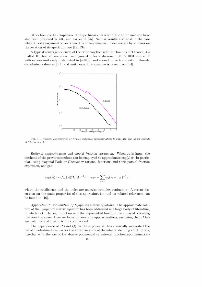
A typical convergence curve of the error together with the bounds of Theorem 4.4(called HL bound) are shown in Figure 4.1, for a diagonal 1001 × 1001 matrix Awith entries uniformly distributed in [−40, 0] and a random vector v with uniformlydistributed values in [0, 1] and unit norm; this example is taken from [34].

0 5 10 15 20 25 30 35 40 45

10−15

10−10

10−5

100

105

dimension of Krylov subspace

no

rm o

f e

rro

r

HL bound

norm of error

Fig. 4.1. Typical convergence of Krylov subspace approximation to exp(A)v and upper bounds

of Theorem 4.4.

Rational approximation and partial fraction expansion. When A is large, themethods of the previous sections can be employed to approximate exp(A)v. In partic-ular, using diagonal Pade or Chebyshev rational functions and their partial fractionexpansion, one gets

exp(A)v ≈ Nν(A)Dν(A)−1v = ω0v +ν∑

j=1

ωj(A − τjI)−1v,

where the coefficients and the poles are pairwise complex conjugates. A recent dis-cussion on the main properties of this approximation and on related references canbe found in [46].

Application to the solution of Lyapunov matrix equations. The approximate solu-tion of the Lyapunov matrix equation has been addressed in a large body of literature,in which both the sign function and the exponential function have played a leadingrole over the years. Here we focus on low-rank approximations, assuming that B hasfew columns and that it is full column rank.

The dependence of P (and Q) on the exponential has classically motivated theuse of quadrature formulas for the approximation of the integral defining P (cf. (4.2)),together with the use of low degree polynomial or rational function approximations

15

to exp(tλ). More precisely, setting X(t) = exp(tA)B, P could be approximated as

P (τ) =

∫ τ

0

X(t)X(t)T dt,

for some τ ≥ 0. Then, by using a quadrature formula with discretization points ti andweights δi, the integral in [0, τ ] is approximated as P (τ) ≈ ∑k

i=1 X(ti)δiX(ti)T . The

practical effectiveness of the approach depends on the value of τ , but most notably onthe quadrature formula used, under the constraint that all δi be positive, to ensure thatP (τ) is positive semidefinite; see [58] for some experiments using different quadratureformulas.

The procedure above determines a low-rank approximation to the correspond-ing Gramian since the number of columns of B is small. An alternative approachthat bypasses the integral formulation within the low-rank framework, is obtainedby reducing the problem dimension. If an approximation to exp(tA)B is available asxk = Vk exp(tHk)E, where E and Vk are defined so that B = VkE, then

Pk = Vk

∫ ∞

0

exp(tHk)EET exp(tHTk )dt V T

k =: VkGkV Tk .

If Hk is stable, Theorem 4.1 ensures that Gk is the solution to the following smalldimensional Lyapunov equation:

HkG + GHTk + EET = 0. (4.3)

This derivation highlights the theoretical role of the exponential in the approximationprocedure. However, one can obtain Gk by directly solving the small matrix equation,by means of methods that exploit matrix factorizations [3], [30].

The following result sheds light onto the reduction process performed by thisapproximation; see, e.g., [39], [58].

Proposition 4.5. Let the columns of Vk, with V Tk Vk = Ik, span Kk(A,B) =

spanB,AB, . . . , Ak−1B. The approximate solution Pk = VkGkV Tk where Gk solves

(4.3) is the result of a Galerkin process onto the space Kk(A,B).Proof. Let Vk be a matrix whose orthonormal columns span Kk(A,B). Let

Rk = APk + PkAT + BBT be the residual associated with Pk = VkGkV Tk for some

Gk and let Hk = V Tk AVk. A Galerkin process imposes the following orthogonality

condition on the residual1

V Tk RkVk = 0.

Expanding Rk and using V Tk Vk = I, we obtain

V Tk AVkGkV T

k + GkV Tk AT Vk + V T

k BBT Vk = 0

HkGk + GkHk + V Tk BBT Vk = 0.

Recalling that B = VkE, the result follows.Other methods have been proposed to approximately solve large-scale Lyapunov

equations; see [28],[44],[55] and references therein.

1This “two-sided” condition can be derived by first defining the matrix inner product 〈X, Y 〉 =tr(XY T ) and then imposing 〈Rk, Pk〉 = 0 for any Pk = VkGV T

kwith G ∈ R

k×k.

16

5. The matrix sign function. In this section we discuss methods for the matrixsign function, with the sign function on C defined as

sign(z) =

+1 if <(z) > 0,−1 if <(z) < 0.

We do not define sign(z) on the imaginary axis where, anyway, it is not continuous.Outside the imaginary axis, sign is infinitely often differentiable, so that sign(A) isdefined as long as the matrix A ∈ C

n×n has no eigenvalues on the imaginary axis. Wefirst recall a few application problems where the sign function is commonly employed.

5.1. Motivation. The algebraic Riccati equation arises in control theory as avery fundamental system to be solved in order to compute, for example, certain ob-servers or stabilizers, see [4], [43]. It is a quadratic matrix equation of the form

G + AT X + XA − XFX = 0, (5.1)

where A,F,G ∈ Rn×n and F and G are symmetric and positive definite. One aims at

finding a symmetric positive definite and stabilizing solution X, i.e. the spectrum ofA − FX should lie in C

−. The quadratic equation (5.1) can be linearized by turningit into a system of doubled size as

K :=

[AT GF −A

]=

[X −II 0

]·[

−(A − FX) −F0 (A − FX)T

]·[

X −II 0

]−1

.

If we assume that X is a stabilizing solution (such a solution exists under mild condi-tions, see [4],[43]), a standard approach is to use the matrix sign function to computeX. We have sign(−(A − FX)) = I and sign(A − FX) = −I. Therefore,

sign

[−(A − FX) −F

0 (A − FX)T

]=

[I Z0 −I

], Z ∈ R

n×n

and we see that

sign(K) − I =

[X −II 0

]·[

0 Z0 −2I

]·[

X −II 0

]−1

. (5.2)

Split sign(K) − I vertically in its middle as [M |N ], move the inverse matrix to theleft-hand side in (5.2) and then equate the first halves, to get

MX = N.

This is an overdetermined, but consistent linear system for X, and by working withthe second half blocks, it can be shown that M is full column rank. Therefore, theprocedure above outlines a method to derive a stabilizing solution X to (5.1) by meansof the sign function.

As discussed in section 4.3, the Lyapunov equation

AT X + XA + CT C = 0, where A,C ∈ Rn×n

also arises in control theory. It was already shown in [57] that the (Hermitian) solutionX is the (2,1) block of the sign-function of a matrix of twice the dimension, that is

[0 0X I

]=

1

2

(I + sign

([A 0

CT C −AT

])).

17

This follows in a way similar to what we presented for the algebraic Riccati equation;see also [5] for a generalization.

The matrix sign function also appears in the modelling (and subsequent simu-lation) of complex physical systems. One example is given by the so-called overlapfermions of lattice quantum chromodynamics [53], where one has to solve linear sys-tems of the form

(I + Γ5sign(Q))x = b. (5.3)

Here Γ5 is a simple permutation matrix and Q is a huge, sparse, complex Hermitianmatrix representing a nearest neighbour coupling on a regular 4-dimensional gridwith 12 variables per grid point. Note that here we may situate ourselves in anorder reduction context, since if we solve (5.3) with some iterative method, the basicoperation will be to compute matrix-vector products, i.e. we need the action sign(Q)vrather than sign(Q) itself.

5.2. Matrix methods. A detailed survey on methods to compute the wholematrix sign(A) is given in [42], see also [2]. We shortly describe the most importantones.

The Newton iteration to solve z2 − 1 = 0 converges to +1 for all starting valuesin the right half plane, and to −1 for all those from C

−. According to (3.5), thecorresponding matrix iteration reads

Sk+1 =1

2

(Sk + S−1

k

), where S0 = A. (5.4)

Although the convergence is global and asymptotically quadratic, it can be quite slowin the presence of large eigenvalues or eigenvalues with a small real part. Therefore,several accelerating scaling strategies have been proposed [41], for example by usingthe determinant [8], i.e.

Sk+1 =1

2

((ckSk) +

1

ckS−1

k

), with ck = det(Sk).

Note that det(Sk) is easily available if Sk is inverted using the LU -factorization. Analternative which avoids the computation of inverses is the Schulz iteration, obtainedas Newton’s method for z−2 − 1 = 0, which yields

Sk+1 =1

2· Sk ·

(3I − S2

k

), S0 = A.

This iteration is guaranteed to converge only if ‖I−A2‖ < 1 (in an arbitrary operatornorm).

In [40], several other iterations were derived, based on Pade approximations ofthe function (1 − z)−1/2. They have the form

Sk+1 = Sk · Nµν(S2k) · Dµν(S2

k)−1, S0 = A.

For µ = 2p, ν = 2p − 1, an alternative representation is

Sk+1 =((I + Sk)2p + (I − Sk)2p

)·((I + Sk)2p − (I − Sk)2p

)−1. (5.5)

18

In this case, the coefficients of the partial fraction expansion are explicitly known,giving the equivalent representation

Sk+1 =1

p· Sk ·

p∑

i=1

1

ξi

(S2

k + αiI)−1

, S0 = A, (5.6)

with ξi =1

2

(1 + cos

(2i − 1)π

2p

), α2

i =1

ξi− 1, i = 1, . . . , p.

Interestingly, ` steps of the iteration for parameter p are equivalent to one stepwith parameter p`. The following global convergence result on these iterations wasproved in [40].

Theorem 5.1. If A has no eigenvalues on the imaginary axis, the iteration (5.5)converges to sign(A). Moreover, one has

(sign(A) − Sk)(sign(A) + Sk)−1 =((sign(A) − A)(sign(A) + A)−1

)(2p)k

,

which, in the case that A is diagonalizable, gives

‖(sign(A)−Sk)(sign(A) + Sk)−1‖ ≤ ‖T‖ · ‖T−1‖ ·(

maxλ∈spec(A)

sign(λ) − λ

sign(λ) + λ

)2pk

. (5.7)

5.3. Krylov subspace approximations. We now look at Krylov subspace ap-proximations for

sign(A)v, v ∈ Cn

with special emphasis on A Hermitian. The Krylov subspace projection approachfrom (3.8) gives

sign(A)v ≈ Vksign(Hk)e1 · ‖v‖. (5.8)

If one monitors the approximation error in this approach as a function of k, thedimension of the Krylov subspace, one usually observes a non-monotone, jig-saw likebehaviour. This is particularly so for Hermitian indefinite matrices, where the realeigenvalues lie to the left and to the right of the origin. This can be explained bythe fact, formulated in Proposition 3.1, that the Krylov subspace approximation isgiven as pk−1(A)v where pk−1 is the degree k − 1 polynomial interpolating at theRitz values. But the Ritz values can get arbitrarily close to 0 (or even vanish), eventhough the spectrum of A may be well separated from 0, then producing a (relatively)large error in the computed approximation. A Ritz value close to 0 is likely to occurif k − 1 is odd, so the approximation has a tendency to degrade every other step.A remedy to this phenomenon is to use the polynomial that interpolates A at theharmonic Ritz values, since these can be shown to be as well separated from zero asspec(A). Computationally, this can be done using the same Arnoldi recurrence (3.7)as before, but applying a simple rank-one modification to Hk before computing itssign function. Details are given in [66].

An alternative is to use the identity

sign(z) = z · (z2)−1

2 ,

19

then use the Krylov subspace approach on the squared matrix A2 to approximate

(A2

)− 1

2 v ≈ Vk(Hk)−1

2 e1 · ‖v‖ =: yk,sign(A)v ≈ xk = Ayk.

(5.9)

Note that in (5.9) the matrix Hk represents the projection of A2 (not of A !),onto the Krylov subspace Kk(A2, b). Interestingly, this is one of the special caseswhen explicitly generating the space Kk(A2, b) is more effective than using Kk(A, b);see [67] for a general analysis of cases when using the latter is computationally moreadvantageous.

It is also remarkable that, in case that A is Hermitian, it is possible to give aposteriori error bounds on the quality of the approximation xk as formulated in thefollowing theorem taken from [66].

Theorem 5.2. Let A be Hermitian and non-singular. Then xk from (5.9) satis-fies

‖sign(A)v − xk‖2 ≤ ‖rk‖2 ≤ 2κ

(κ − 1

κ + 1

)k

· ‖v‖2, (5.10)

where κ ≡ ‖A‖2‖A−1‖2 and rk is the residual in the k-th step of the CG methodapplied to the system A2x = v (with initial residual v, i.e. initial zero guess).

The residual norms ‖rk‖ need not be computed via the CG method since theycan be obtained at almost no cost from the entries of the matrix Hk in the Lanczosrecursion (3.7). This can be seen as follows: Since A2 is Hermitian, Hk is Hermitianand tridiagonal. If pk−1 is the degree k − 1 polynomial expressing the k-th Lanczosvector vk as vk = pk−1(A

2)v, the Lanczos recursion gives hk+1,kpk(z) = (z − hk,k) ·pk−1(z) − hk−1,kpk−2(z). On the other hand, it can be shown that rk = σvk+1 with‖vk+1‖ = 1 for some scalar σ (see [60, Proposition 6.20]), and since rk = qk(A2)v forsome polynomial qk of degree k satisfying qk(0) = 1, it must be qk = pk/pk(0), sothat rk = pk(A2)v/pk(0) = vk+1/pk(0). Therefore, along with the Lanczos process wejust have to evaluate the recursion pk(0) = −[hk,k · pk−1(0) + hk−1,kpk−2(0)]/hk+1,k

to obtain ‖rk‖ = 1/|pk(0)|.We do not know of comparable error bounds for the other two approaches outlined

earlier ((5.8) and its variant using harmonic Ritz values). Note also that xk from (5.9)satisfies xk = Apk−1(A

2)v, where q(z) = z · pk−1(z2) is an odd polynomial, that is

q(−z) = −q(z), of degree 2k−1 in z. This is a restriction as compared to the other twoapproaches where we do not enforce any symmetry on the interpolating polynomials.However, this restriction will most probably have an effect only if the spectrum ofA is very unsymmetric with respect to the origin. Our computational experiencein simulations from lattice QCD indicates that xk is actually the best of the threeapproximations discussed so far. Since, in addition, xk comes with a bound of thetrue error norm, we definitely favor this approach.

5.4. Partial fraction expansions. If we have sufficient information on theeigensystem of A available, we can use (5.7) to estimate a number p ∈ N such thatthe first iterate from (5.6) already gives a sufficiently good approximation to the signfunction. As discussed in section 3.6, we can then approximate

sign(A)v ≈ A ·p∑

i=1

1

pξix(j),

20

with x(j) an approximate solution of the linear system

(A2 + αjI)x(j) = v, j = 1, . . . , p.

We already discussed in section 3.6 how we can make efficient use of the shifted natureof these systems when solving them with standard Krylov subspace methods.

A particularly important situation arises when A is Hermitian and the inter-vals [−b,−a] ∪ [c, d], with 0 < a ≤ b, 0 < c ≤ d, containing the eigenvalues of Aare available. Under these hypotheses, Zolotarev explicitly derived the best ratio-nal approximation in the Chebyshev sense; see [56]. The next theorem states thisresult for [−b,−a] = −[c, d]. The key point is that for fixed µ = 2p − 1, ν = 2p,finding the optimal rational approximation Rµν(z) = Nµν(z)/Dµν(z) to the signfunction on [−b,−a]∪ [a, b] is equivalent to finding the best such rational approxima-tion Sp−1,p(z) = Np−1,p(z)/Dp−1,p(z) in relative sense to the inverse square root on[1, (b/a)2]. The two functions are then related via R2p−1,2p(z) = az · Sp−1,p(az).

Proposition 5.3. Let R2p−1,2p(z) = N2p−1,2p(z)/D2p−1,2p(z) be the Chebyshevbest approximation to sign(z) on the set [−b,−a] ∪ [a, b], i.e. the function whichminimizes

maxa<|z|<b

|sign(z) − R2p−1,2p(z)|

over all rational functions R2p−1,2p(z) = N2p−1,2p(z)/D2p−1,2p(z). Then the factoredform of R2p−1,2p is given by

R2p−1,2p(z) = az · Sp−1,p((az)2) with Sp−1,p(z) = D

∏p−1i=1 (z + c2i)∏p

i=1(z + c2i−1),

where

ci =sn2

(iK/(2p);

√1 − (b/a)2

)

1 − sn2(iK/(2p);

√1 − (b/a)2

) ,

K is the complete elliptic integral, sn is the Jacobi elliptic function, and D is uniquelydetermined by the condition

maxz∈[1,(b/a)2]

(1 −√

zSp−1,p(z))

= − minz∈[1,(b/a)2]

(1 −√

zSp−1,p(z)).

For a given number of poles, the Zolotarev approximation is much more accuratethan that of the rational approximation (5.6) and is therefore to be preferred. Thisis illustrated in Table 5.1, taken form [66]. However, the use of the Zolotarev approx-imation is restricted to Hermitian matrices for which lower and upper bounds (a andb, resp.) on the moduli of the eigenvalues are known.

As a final point, let us again assume that A is Hermitian and that we approxi-mate sign(A) by some rational approximation R(A) with R having a partial fractionexpansion of the form

R(z) =

p∑

j=1

ωjz

z2 + αj, ωj ≥ 0, αj ≥ 0, j = 1, . . . , p.

21

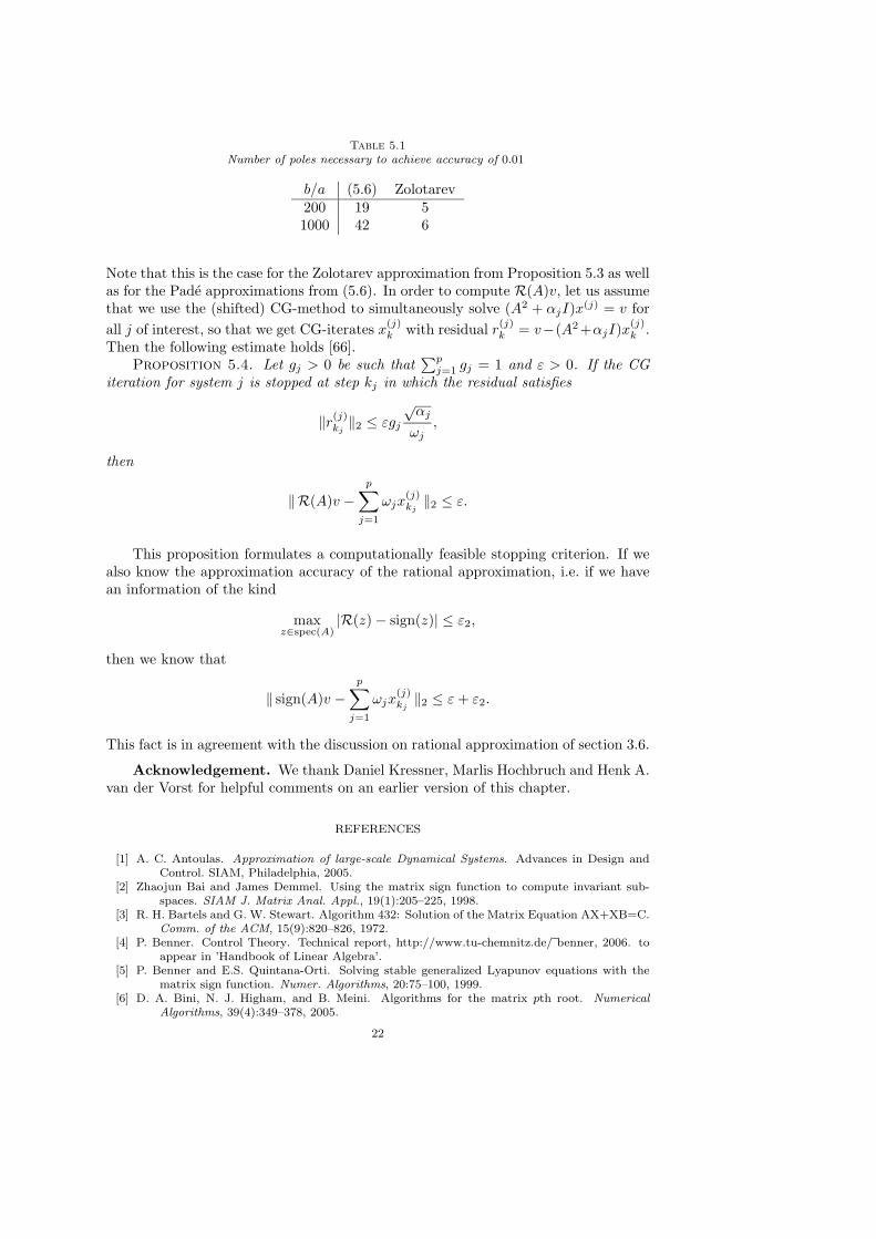
Table 5.1Number of poles necessary to achieve accuracy of 0.01

b/a (5.6) Zolotarev200 19 51000 42 6

Note that this is the case for the Zolotarev approximation from Proposition 5.3 as wellas for the Pade approximations from (5.6). In order to compute R(A)v, let us assumethat we use the (shifted) CG-method to simultaneously solve (A2 + αjI)x(j) = v for

all j of interest, so that we get CG-iterates x(j)k with residual r

(j)k = v−(A2+αjI)x

(j)k .

Then the following estimate holds [66].Proposition 5.4. Let gj > 0 be such that

∑pj=1 gj = 1 and ε > 0. If the CG

iteration for system j is stopped at step kj in which the residual satisfies

‖r(j)kj

‖2 ≤ εgj

√αj

ωj,

then

‖R(A)v −p∑

j=1

ωjx(j)kj

‖2 ≤ ε.

This proposition formulates a computationally feasible stopping criterion. If wealso know the approximation accuracy of the rational approximation, i.e. if we havean information of the kind

maxz∈spec(A)

|R(z) − sign(z)| ≤ ε2,

then we know that

‖ sign(A)v −p∑

j=1

ωjx(j)kj

‖2 ≤ ε + ε2.

This fact is in agreement with the discussion on rational approximation of section 3.6.

Acknowledgement. We thank Daniel Kressner, Marlis Hochbruch and Henk A.van der Vorst for helpful comments on an earlier version of this chapter.

REFERENCES

[1] A. C. Antoulas. Approximation of large-scale Dynamical Systems. Advances in Design andControl. SIAM, Philadelphia, 2005.

[2] Zhaojun Bai and James Demmel. Using the matrix sign function to compute invariant sub-spaces. SIAM J. Matrix Anal. Appl., 19(1):205–225, 1998.

[3] R. H. Bartels and G. W. Stewart. Algorithm 432: Solution of the Matrix Equation AX+XB=C.Comm. of the ACM, 15(9):820–826, 1972.

[4] P. Benner. Control Theory. Technical report, http://www.tu-chemnitz.de/ebenner, 2006. toappear in ’Handbook of Linear Algebra’.

[5] P. Benner and E.S. Quintana-Orti. Solving stable generalized Lyapunov equations with thematrix sign function. Numer. Algorithms, 20:75–100, 1999.

[6] D. A. Bini, N. J. Higham, and B. Meini. Algorithms for the matrix pth root. Numerical

Algorithms, 39(4):349–378, 2005.

22

[7] P. B. Borwein. Rational approximations with real poles to e−x and xn. Journal of Approxi-

mation Theory, 38:279–283, 1983.[8] R. Byers. Solving the algebraic Riccati equation with the matrix sign function. Linear Algebra

Appl., 85:267–279, 1987.[9] A. J. Carpenter, A. Ruttan, and R. S. Varga. Extended numerical computations on the “1/9”

conjecture in rational approximation theory. In P. R. Graves-Morris, E. B. Saff, andR. S. Varga, editors, Rational approximation and interpolation. Proceedings of the United

Kingdom-United States conference held at Tampa, Florida, December 12-16, 1983, pages503–511, Berlin, 1990. Springer-Verlag, Lecture Notes Math.

[10] E. Celledoni and A. Iserles. Approximating the exponential from a Lie algebra to a Lie group.Mathematics of Computation, 69(232):1457–1480, 2000.

[11] E. Celledoni and I. Moret. A Krylov projection method for systems of ODEs. Applied Num.

Math., 24:365–378, 1997.[12] W. J. Cody, G. Meinardus, and R. S. Varga. Chebyshev rational approximations to e−x in

[0, +∞) and applications to heat-conduction problems. J. Approx. Theory, 2(1):50–65,March 1969.

[13] M. J. Corless and A. E. Frazho. Linear systems and control - An operator perspective. Pureand Applied Mathematics. Marcel Dekker, New York - Basel, 2003.

[14] Ph. I. Davies and N. J. Higham. Computing f(A)b for matrix functions f . In QCD and

numerical analysis III, volume 47 of Lect. Notes Comput. Sci. Eng., pages 15–24. Springer,Berlin, 2005.

[15] P. J. Davis and P. Rabinowitz. Methods of Numerical Integration. Academic Press, London,2nd edition edition, 1984.

[16] J. W. Demmel. Applied numerical linear algebra. SIAM, Philadelphia, 1997.[17] V. Druskin, A. Greenbaum, and L. Knizhnerman. Using nonorthogonal Lanczos vectors in the

computation of matrix functions. SIAM J. Sci. Comput., 19(1):38–54, 1998.[18] V. Druskin and L. Knizhnerman. Two polynomial methods of calculating functions of sym-

metric matrices. U.S.S.R. Comput. Math. Math. Phys., 29:112–121, 1989.[19] V. Druskin and L. Knizhnerman. Extended Krylov subspaces: approximation of the matrix

square root and related functions. SIAM J. Matrix Analysis and Appl., 19(3):755–771,1998.

[20] M. Eiermann and O. Ernst. A restarted Krylov subspace method for the evaluation of ma-trix functions. Technical report, Institut fur Numerische Mathematik und Optimierung,Technische Universitat Bergakademie Freiberg, 2005.

[21] R. W. Freund. Solution of shifted linear systems by quasi-minimal residual iterations. InL. Reichel et al., editor, Numerical linear algebra. Proceedings of the conference in numer-

ical linear algebra and scientific computation, Kent, OH, USA, March 13-14, 1992, pages101–121. Walter de Gruyter, Berlin, 1993.

[22] A. Frommer. BiCGStab(`) for families of shifted linear systems. Computing, 70:87–109, 2003.[23] A. Frommer and U. Glassner. Restarted GMRES for shifted linear systems. SIAM J. Sci.

Comput., 19(1):15–26, 1998.[24] A. Frommer and P. Maass. Fast CG-based methods for Tikhonov–Phillips regularization. SIAM

J. Sci. Comput., 20(5):1831–1850, 1999.[25] E. Gallopoulos and Y. Saad. Efficient solution of parabolic equations by Krylov approximation

methods. SIAM J. Sci. Stat. Comput., 13(5):1236–1264, 1992.[26] W. Gautschi. Numerical Analysis. An Introduction. Birkhauser, Boston, 1997.[27] G. Golub and C. F. Van Loan. Matrix computations. The Johns Hopkins Univ. Press, Baltimore,

3rd edition, 1996.[28] S. Gugercin, D. C. Sorensen, and A. C. Antoulas. A modified low-rank Smith method for

large-scale Lyapunov equations. Numer. Algorithms, 32:27–55, 2003.[29] E. Hairer, C. Lubich, and G. Wanner. Geometric numerical integration. Structure-preserving

algorithms for ordinary differential equations, volume 31 of Springer Series in Computa-

tional Mathematics. Springer, Berlin, 2002.[30] S. J. Hammarling. Numerical solution of the stable, non-negative definite Lyapunov equation.

IMA J. Numer. Anal., 2:303–323, 1982.[31] N. J. Higham. Newton’s method for the matrix square root. Math. Comp., 46(174):537–549,

April 1986.[32] N. J. Higham. Stable iterations for the matrix square root. Numer. Algorithms, 15(2):227–242,

1997.[33] N. J. Higham. The Scaling and Squaring Method for the Matrix Exponential Revisited. SIAM

J. Matrix Analysis and Appl., 26(4):1179–1193, 2005.[34] M. Hochbruck and C. Lubich. On Krylov subspace approximations to the matrix exponential

23

operator. SIAM J. Numer. Anal., 34(5):1911–1925, 1997.[35] M. Hochbruck, C. Lubich, and H. Selhofer. Exponential integrators for large systems of differ-

ential equations. SIAM J. Sci. Comput., 19(5):1552–1574, 1998.[36] M. Hochbruck and J. van den Eshof. Preconditioning Lanczos approximations to the matrix

exponential. SIAM J. Sci. Comput., 27(4):1438–1457, 2006.[37] R. A. Horn and C. R. Johnson. Topics in matrix analysis. 1st paperback ed. with corrections.

Cambridge University Press, Cambridge, 1994.[38] A. Iserles, H. Z. Munthe-Kaas, S. P. Nørsett, and A. Zanna. Lie-group methods. Acta Numerica,

9:215–365, 2000.[39] I. M. Jaimoukha and E. M. Kasenally. Krylov subspace methods for solving large Lyapunov

equations. SIAM J. Numer. Anal., 31(1):227–251, Feb. 1994.[40] C. Kenney and A. J. Laub. Rational iterative methods for the matrix sign function. SIAM J.

Matrix Anal. Appl., 12(2):273–291, 1991.[41] C. Kenney and A. J. Laub. On scaling Newton’s method for polar decomposition and the

matrix sign function. SIAM J. Matrix Anal. Appl., 13(3):688–706, 1992.[42] C. S. Kenney and A. J. Laub. The matrix sign function. IEEE Trans. Autom. Control,

40(8):1330–1348, 1995.[43] P. Lancaster and L. Rodman. The Algebraic Riccati Equation. Oxford University Press, Oxford,

2nd edition edition, 1995.[44] J.-R. Li and J. White. Low-Rank solutions of Lyapunov equations. SIAM Review, 46(4):693–

713, 2004.[45] Charles Van Loan. The sensitivity of the matrix exponential. SIAM J. Numer. Anal., 14(6):971–

981, 1977.[46] L. Lopez and V. Simoncini. Analysis of projection methods for rational function approximation

to the matrix exponential. SIAM J. Numer. Anal., 44(2):613 – 635, 2006.[47] L. Lopez and V. Simoncini. Preserving geometric properties of the exponential matrix by block

Krylov subspace methods. Technical report, Dipartimento di Matematica, Universita diBologna, December 2005.

[48] The MathWorks, Inc. MATLAB 7, September 2004.[49] C. Moler and C. Van Loan. Nineteen dubious ways to compute the exponential of a matrix,

twenty-five years later. SIAM Review, 45(1):3–49, 2003.[50] I. Moret and P. Novati. An interpolatory approximation of the matrix exponential based on

Faber polynomials. J. Comput. and Applied Math., 131:361–380, 2001.[51] I. Moret and P. Novati. RD-rational approximations of the matrix exponential. BIT, Numerical

Mathematics, 44(3):595–615, 2004.[52] I. Moret and P. Novati. Interpolating functions of matrices on zeros of quasi-kernel polynomials.

Numer. Linear Algebra Appl., 11(4):337–353, 2005.[53] H. Neuberger. The overlap Dirac operator. In Numerical Challenges in Lattice Quantum

Chromodynamics, volume 15 of Lect. Notes Comput. Sci. Eng., pages 1–17. Springer,Berlin, 2000.

[54] S. P. Nørsett. Restricted Pade approximations to the exponential function. SIAM J. Numer.

Anal., 15(5):1008–1029, Oct. 1978.[55] T. Penzl. A cyclic low-rank Smith method for large sparse Lyapunov equations. SIAM J. Sci.

Comput., 21(4):1401–1418, 2000.[56] P. P. Petrushev and V. A. Popov. Rational approximation of real functions. Cambridge

University Press, Cambridge, 1987.[57] J. D. Roberts. Linear model reduction and solution of the algebraic Riccati equation by use of

the sign function. Int. J. Control, 32:677–687, 1980.[58] Y. Saad. Numerical solution of large Lyapunov equations. In M. A. Kaashoek, J. H. van

Schuppen, and A. C. Ran, editors, Signal Processing, Scattering, Operator Theory, and

Numerical Methods. Proceedings of the international symposium MTNS-89, vol III, pages503–511, Boston, 1990. Birkhauser.

[59] Y. Saad. Analysis of some Krylov subspace approximations to the matrix exponential operator.SIAM J. Numer. Anal., 29:209–228, 1992.

[60] Y. Saad. Iterative Methods for Sparse Linear Systems. The PWS Publishing Company, Boston,1996. Second edition, SIAM, Philadelphia, 2003.

[61] R. B. Sidje. Expokit: A Software Package for Computing Matrix Exponentials. ACM Trans-

actions on Math. Software, 24(1):130–156, 1998.[62] V. Simoncini and D. B. Szyld. Recent developments in Krylov subspace methods for linear

systems. Technical report, Dipartimento di Matematica, Universita di Bologna, September2005. Submitted.

[63] D. E. Stewart and T. S. Leyk. Error estimates for Krylov subspace approximations of matrix

24

exponentials. J. Comput. and Applied Math., 72:359–369, 1996.[64] H. Tal-Ezer. Spectral methods in time for parabolic problems. SIAM J. Numer. Anal., 26:1–11,

1989.[65] L. N. Trefethen, J. A. C. Weideman, and T. Schmelzer. Talbot Quadratures and Rational

Approximations. BIT, to appear.[66] J. van den Eshof, A. Frommer, Th. Lippert, K. Schilling, and H.A. van der Vorst. Numerical

methods for the QCD overlap operator. I: Sign-function and error bounds. Comput. Phys.

Commun., 146(2):203–224, 2002.[67] H.A. van der Vorst. An iterative solution method for solving f(A)x = b, using Krylov subspace

information obtained for the symmetric positive definite matrix A. J. Comput. Appl. Math.,18:249–263, 1987.

[68] Henk A. van der Vorst. Solution of f(A)x = b with projection methods for the matrix A.In Numerical Challenges in Lattice Quantum Chromodynamics, volume 15 of Lect. Notes

Comput. Sci. Eng., pages 18–28. Springer, Berlin, 2000.[69] R. S. Varga. On higher order stable implicit methods for solving parabolic partial differential

equations. J. of Mathematics and Physics, XL:220–231, 1961.[70] A. Zanna and H. Z. Munthe-Kaas. Generalized polar decompositions for the approximation of

the matrix exponential. SIAM J. Matrix Analysis and Appl., 23(3):840–862, 2002.

25