2 testing the reliability and existence - gulzar

DOI: 10.31703/ger.2019(IV-II).02 URL: http://dx.doi.org/10.31703/ger.2019(IV-II).02

Gulzar Ali * | Said Zamin Shah † | Ghulam Mustafa ‡

Testing the Reliability and Existence of IS-LM Model for Pakistan

The IS-LM model was considered indispensable and

had great importance and recital for macroeconomic phenomenon at theoretical as well empirical analysis since 1960s. Now a days the applications of IS-LM model has been greatly restricted to few situations depicts losing the fame. However, it has been a crucial part of the basic principles and manuscripts of macroeconomics long since 1960s. Observing the reliability and existence of IS-LM model in case of Pakistan, for that purpose the study regressed two model; in first the basic model without including the model parameters and in second, with model parameters. The empirical results found the reliability and existence of IS-LM model.

JEL Classification E44, E41, E21

• Vol. IV, No. II (Spring 2019)

• Page: 13 – 23

• p-ISSN: 2521-2974

• e-ISSN: 2707-0093

• L-ISSN: 2521-2974

Key Words: IS-LM model, planned expenditure, Descriptive Statistics, ARDL approach.

Introduction IS-LM analysis is a philosophical phenomenon, and to realize its determination one should be aware of the principles of basic economic theory (Casares and McCallum, 2006). The IS-LM theory was considered indispensable and had great performance at both empirical and theoretical analysis of macroeconomic phenomenon since 1960s, however the thought didn’t persists now, which indicates the chronological changes in the model during last century according to requirements of situation. Now a days the applications of IS-LM model has been greatly restricted to few situations depicts losing the fame. However it has been a crucial part of the basic principles and manuscripts of macroeconomics long since 1960s. Even though the Aggregate Expenditure or Aggregate Production formation of the IS-LM model is vanishing from the macro-economic manuscript and is being swapped with Aggregate Supply or Aggregate Demand model. One of the interesting features of this advancement is that, in principle, the Aggregate Supply or Aggregate Demand model is the derivation result of IS-LM framework. Previously, the Aggregate Expenditure or Aggregate Production multiplier model, that

*Assistant Professor, Department of Economics, Islamia College Peshawar, KP, Pakistan.Email: [email protected]

†Assistant Professor, Department of Economics, Islamia College Peshawar, KP, Pakistan.‡Assistant Professor, Department of Economics and Business Administration, Division of Artsand Social Sciences, University of Education, Lahore, Punjab Pakistan.

Abstract

Gulzar Ali, Said Zamin Shah and Ghulam Mustafa

Page | 14 Global Economics Review (GER)

is fundamental part of IS-LM model formation, appeared to be the compulsory part of the macro-economic texts and principles, and the IS-LM transitional model was the expansion of the basic Aggregate Expenditure or Aggregate Production model. Currently, the model multiplier has lost its importance from the basic principles of macro-economics, and has been replaced with the Aggregate Supply or Aggregate Demand based analysis with strong theoretical grounds and significant empirical applications. Furthermore fewer references of the IS-LM model observed in top journals shows the limited scope of the discussion in the contemporary theory.

Efforts have been done by (Clarida et al., 1999; and Yun, 1996) to interpret modern research and theory in context of IS-LM framework. However their models are based upon the dynamic general equilibrium model, and the transformation their models in IS-LM is not fundamental part of their study. The transformation is just operated by policy concerned to provide mean of connecting their outcomes to IS-LM framework. Colander and Gamber (2002) presented dynamic general equilibrium models by assuming minor inflexibilities; a transitory negative association can possibly be seen between interest rates and output growth that is be named “IS” curve. The model has been closed by an arrangement of nominal interest rates instead of a traditional LM curve; however that difference is nominal that is associated with standard IS-LM model via introducing effectual LM curve into the model that integrates the monetary reaction.

The present situation is almost opposite to that of 1960s where IS-LM model has been the focal point of both theoretical and policy debates and discussions. IS-LM was at the core of the macro-economic offering a combination of Keynesian and classical models, which were a key factor in politics and higher education on the economy. If someone had learned IS-LM in 1960s, then there was no huge leap between advance macroeconomic work and intermediate studies. Till mid 1970s the IS-LM was basics of the graduate economics course. Nowadays the debate about multiple market items and the equilibrium of money market lost the focus to great extent, and IS-LM is merely used just as a framework for policy argument, indicating that IS-LM continued, but its function has altered significantly.

In the 1960s, the IS-LM model was highlighted not only as the starting point for a theoretical macroeconomics, but it was also the basics for the overall empirical macroeconomic and econometric models which was then the focal point of advance macroeconomic policy analysis. In 1960s the application of IS-LM was extended to large econometric models which had hundreds of equations however the structure of those equations remained the same. Lawrence (2000) represented the educational use of the IS-LM in a very good and revealed how IS-LM model could be presented with empirical contents in view of its role in past and assuming the same performance for present situation. It is recommended by him that “systems that are carefully fitted to observed data and capable of generating realistic values are far better for teaching purposes.” The statement is accurate but it doesn’t represent the case of IS-LM in the advance analysis as profession is more apprehensive of the economic models on a large scale and the consequence derived are ambiguous while dealing with real situation.

Various researches have efficiently used active macro-economic models having enhancing comportment articulated in the form of associations that were alike in numerous aspects to conventional models of the IS-LM (i.e. Woodford, 2003; Gali and Gertler, 1999; Jeanne, 1998; Walsh, 1998; Woodford, 1995). The major differentiation among the models of the cited studies and traditional IS-LM formation is the differentiation of interest rates (real and nominal) and the accompaniment of IS function


Vol. IV, No. II (Spring 2019) Page | 15

that contains extra term concerning to the anticipated expenditure in future. In addition of the term provides futuristic feature of expenditure assessments, an aspect that in general consequence in considerably changed dynamic performance in the model, comparative to the traditional kind. Yet, optimizing models have considerable restrictions, among which a most noteworthy is that capital investment is generally considered to be exogenous (McCallum and Nelson; 1999) or absent (Woodford; 1995). Obviously, this limitation is pretty considerable. Besides ignoring the opportunity of investigating matters concerning the growth and capital formation, however it also eliminates the chance of describing endogenously the complementary changeability of investment/speculative and consumption expenditure, a distinction characterized in most of the literature related to real-business- cycle (Gali; 2001).

From the above discussion it can be concluded that though IS-LM model and its existence had remained an important debate for the academic teachers and learners as well as for policy makers and economist. Still IS-LM model has essential place in economic activities by covering both fiscal and monetary policy side. Both the government and financial institution of the country used IS-LM model in development and frameworks of the different policies to be implemented. Keeping the importance of IS-LM model, the existence of IS-LM model and test their reliability through planned expenditure for Pakistan from 1980-2018 to be examined. This empirical attempt may be helpful for an economic agents and policy maker in implementing and making both the monetary and fiscal policies. It will give direction for taking the decision regarding money supply, interest rate, government expenditure, implementation of taxes and propensity change to consumption and possible role in growth. Developing of Empirical Model and Theoretical Justification

This research paper aims to empirically analyze the reliability of IS-LM (Planned expenditure) in case of Pakistan, for that purpose on the basis of above brief theoretical introduction, consider the IS-LM model as;

Consumption functions = a + b(Y - T)……… (1) Investment function: I = c – dr……………….. (2) The sign of Parameters is (a > 0, 0 < b < 1, c > 0, d > 0,) As the Planned expenditure is Y = C + I + G……………………….. (3) Now by putting the value of equations (1) and (2) in to equation (3), it becomes as Y = (a + b (Y - T)) + (c - dr) + G………………………. (3.1) Y (1 - b) = a - bT + c - dr + G…………………………… (3.2) Y = (a- bT + c- dr + G)/ (1-b)……………………………. (3.3) From equation (3.3) the slope of IS curve will be; Slope of IS curve = dY/ dr= -d/ (1-b)…………………………… (3.3a) d[IS(r)]/d(d) = -1/(1-b) < 0…………………(3.3b) As the real demand for money, that is the function of interest rate (r) and income (y)

that is (M/P) = L(r, Y) = (eY-fr)……………………………. (4) fr = (eY-M/P)……………….…………(4.1) r = (eY-M/P)/f……………….………. (4.2) The slope of LM curve sensitivity to the parameters of interest rate to money

demands function, that is;



r = (eY-M/P)/f……………………….. (4.2a) Slope of LM r = dy/dr= e/f ……………………..… (4.2b)

dy/df= -e/f2………………………… (4.2c)

Note that as “f” gets larger, money demand becomes increasingly sensitive (flatter) to interest rate. If LM is more sensitive to real interest rates than “∆r” responds less strongly to changes in income to achieve money market equilibrium; with some ∆Y, smaller r needed to return to equilibrium. Mathematically

dy/dM= d/ {1+(e/f)-p2f}…………………………………………………(5) dy/dM = d/ P{(1-b)f+de}= 1/ P{e +(1-b/d)f} > 0………………………..(5.1) dy/dG= 1/ {1+(de/f)-b} = f/de+(1-b)/f} > 0……………………………(5.2) dy/dT= -b/ {1+(de/f)-b} = -be/de+(1-b)/f} < 0………………………….(5.3) For reliability of planned expenditure, compare equation (3.3) and (4.2), that is; (eY-M/P)/f = -(Y( 1-b) -a+bT-c-G)/d ……………..………………………..(6) By re-arranging equation (6)

eY/f +Y(1-b)/d = ( a-bT +c +G)/d +M/Pf …………………………….……….(6.1) Y( e/f +(1-b)/d) =( a-bT +c +G)/d +M/Pf ……………………………………..(6.2) Y =1/P* (M/f) / ( e/f +(1-b)/d) + ( a-bT +c +G)/d( e/f +(1-b)/d) ……………..(6.3)

The above equation (6.3) shows that planned expenditure or aggregate demand (Y) is the function of P, exogenous variables M, G, and T. whereas “f”, “e”, “b”, “c” and “d” are the model’s parameters.

Analysis, Findings and Discussions

Statistical Description and Normality of the Data

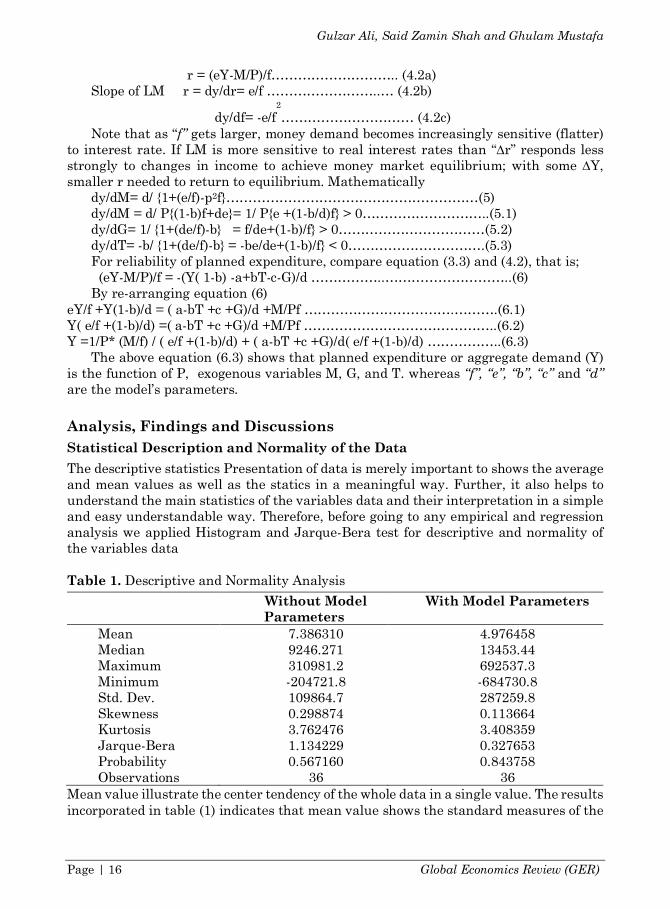
The descriptive statistics Presentation of data is merely important to shows the average and mean values as well as the statics in a meaningful way. Further, it also helps to understand the main statistics of the variables data and their interpretation in a simple and easy understandable way. Therefore, before going to any empirical and regression analysis we applied Histogram and Jarque-Bera test for descriptive and normality of the variables data Table 1. Descriptive and Normality Analysis

Without Model Parameters

With Model Parameters

Mean 7.386310 4.976458 Median 9246.271 13453.44 Maximum 310981.2 692537.3 Minimum -204721.8 -684730.8 Std. Dev. 109864.7 287259.8 Skewness 0.298874 0.113664 Kurtosis 3.762476 3.408359 Jarque-Bera 1.134229 0.327653 Probability 0.567160 0.843758 Observations 36 36

Mean value illustrate the center tendency of the whole data in a single value. The results incorporated in table (1) indicates that mean value shows the standard measures of the



whole variables data used in this study as well as center distribution of the data in descriptive analysis of both (Model without and with Parameters) models.

Central tendency is mainly measures by median in the data. But median is affected if there are any outliers and unusual values included in the variables data. If there is any sort of outliers or unusual values problem in the data, than median is not a best measurement to represent data in the meaningful and descriptive form. The table (1) clarifies that median is represent the data used in this study in their best form thus rejecting any chances of outliers and unusual values in the data. Further, the median also expresses that the data used in the study is preeminent.

In statistical description the data is further elaborated by measuring the range of dispersion using range of variance and standard deviation. The value of standard deviation falls close to the mid-range by comparing the maximum and minimum values assumed by both models as shown in table (1). Skewness shows the probability distribution of the variables as well as error term or random term and it can assume either negative or positive values. Further, Skewness shows and measures symmetry in the data or lack of symmetry. The zero (0) 0f skewness shows that data is perfectly symmetry and if the value of skewness falls between one (1) and zero (0) that indicates that the data set used is symmetry. The simple formula for the skewness that is regressed and considered by most of economic and statistical software is in the form

Skewness= "("$%)("$')

∑ ()$ź)+,

= "+,("$%)("$')

…………………… (7) However, it is too difficult to exactly interpret and Skewness has assumed positive

values and very close to zero for both models (without and with Parameters) showing the data used in this study is properly symmetry of both the models. Moreover, Kurtosis measures the degree of distributed peakedness in the data and the value of Kurtosis assumed the distributed peakedness.

The study also regressed Jarque-Bera test for the normality that either the data is normally distributed as well as normality and correlation between Skewness and kurtosis in the model. The general form of Jarque-Bera test in the regression analysis is

Jarque-Bera = "$-.%/

(𝑠' %2(𝑘𝑡 − 3) …………………… (8)

The results of Jarque-Bera test and their probability values captures normal distribution indicating that variable data is normally distributed and didn’t show any serious problem.

Integration of Sationarity

Shrestha and Chowdhury (2005) concluded that a conspicuous that a negligible alteration in the data specification as well as in assumptions may effectively manipulate and change the outcomes and sometimes non-stationarity that alters the significant results of the variables to spurious, insignificant and biased. Consequently, if the variables data shows their stationarity but still there remains a risk of mis-specification. Non-stationarity has keen suspicious for researchers and investigator while doing research on time series data, as this investigation is also doing on time series analysis so been tested for unit root and the findings showing the rejection of null hypothesis at different level of integration specified below.



Table 2. Stationarity Level Results Variables Acronyms Without Model Parameters With Model Parameters

At I(0) At 1(1) Critical Values

At I(0) At 1(1) CriticalValues

Planned Expenditure

Y -1.889012

-4.945417*

-2.945842

-- -- --

Government Expenditure

G -3.784680*

-6.724531*

-2.945842

-3.477860*

-5.678959*

-2.951125

Taxes T -4.983063*

-7.736903*

-2.945842

-2.213937 -4.475638*

-2.951125

Money Supply

M -1.744261 -4.108121*

-2.945842

-1.676608 -3.821911*

-2.951125

Price Level Index

P -2.127776 -4.032559*

-2.945842

-3.890167*

-6.701775*

-2.951125

Marginal Propensity to Consume

MPC -- -- -- -1.630152 -3.594049 -2.951125

Autonomous Investment

I0 -- -- -- -3.578214 -5.293643 -2.951125

Investment Sensitivity to r

Ir -- -- -- -1.897352 -4.708319 -2.951125

(*) shows rejection of null hypothesis at 5%

1.1. Modeling and Interpretation of Regression Results

Inspect the reliability and existence of IS-LM model, the ARDL approach as technique of regression is applying based on the findings of the stationarity outcomes of table (2). The study regressed two model, one is the basic model without including the variables parameters; i.e.

Y= f (M, G, T, P)……………………………………. (12) Equation (12) shows the theoretical model in which “Y” is the planned expenditure

“M” is the money supply, “G” is the government expenditure, “T” is the taxes and “P” is the price level. The econometric model (without model Parameters) is

The sign of co-efficient estimator that shows the impact and relation of regressor

with dependent variables be;

The ARDL model (without model Parameters) that be regressed for variables data to empirically examined the reliability of planned expenditure from IS-LM model

The second model that is regressed includes the model parameters as assumed by final model (6.3) after deriving. The theoretical and econometric form of that model is

Y= f (M*e/f, G, T, P, c, I0, I0*dr) The econometric model is

0 1 2 3 4 ..................................................(13)t t t t t tY G T M Pa a a a a µ= + + + + +

1 2 3 40, 0, 0, 0,a a a a> > > <

0 2 2 3 4 0 1 2 3

4 ...............................................................................................(1

t n t n t n t n

t t t t t t i t i t i t it i t i t i t i

t n

t i tt i

Y G T M P Y G T M

P

a a a a a b a a a

a h

= = = =

- - - -- - - -

=

--

= + + + + + D + D + D + D

+ D +

å å å å

å 4)

0 1 2 3 4 5 6 0 7*( / ) *( ) ................................(15)t t t t t t t tY M e f G T P c I I drb b b b b b b b µ= + + + + + + + +



In the above econometric model Planned expenditure (Y) is the dependent variable, whereas, independent variables is money supply “M” that is the function of money demand to income (e) and interest rate (f), government expenditure (G), Taxes (T), Marginal propensity to consume (c), autonomous Investment (I0) and Investment that is function of interest rate (dr), regressed model is

Both the models were regressed, in first the basic variables without including model parameters (14) and in the second model with models parameters (16) to empirically examine the reliability of planned expenditure deriving from IS-LM model. ARDL acquire satisfactory number of lags for the regression. The automatic lag length criteria following Akaike Information Criteria (AIC) for both the models (without and with model parameters) and the models were regressed a number of times testing at different level is selected. The optimal lag number that gives best results as well as shows minimum number of lag length was at (1, 0, 1, 1, 0) for the model without including parameters and (1, 1, 0, 0, 1, 0, 1, 1) for the models that include parameters.

The first model with basic variables that doesn’t contains model parameters as derived from IS-LM model in equation (14); the performance of the model is noteworthy as the prob. F-stat is highly significant. Moreover, R2 value enlightens the satisfactory variation between variables included in the model. Table 3. Analysis of the Variables (Without Model Parameters) Variables Co-efficient Sd. Error t-Stat P. values

Constant C -0.412383 0.184085 -2.240169 0.0372 Government Expenditure

G 0.329815 0.474459 0.695139 0.4954


G(-1) 0.273602 0.098712 2.772041 0.0121

Taxes T 0.386571 0.098110 3.940161 0.0009 Money Supply

M 0.275001 0.251972 1.091395 0.2887

Money Supply

M(-1) 0.313073 0.258425 1.211463 0.2406

Price Level P -0.104275 0.053851 -1.936391 0.0678 Price Level P(-1) -0.134815 0.069452 1.941109 0.0672 Lag Value of Y

Y(-1) 0.572877 0.142027 4.033582 0.0007

R2 0.963128 DW 1.797640 Ad. R2 0.936248 F-stat. Prob 0.000000

The result of explanatory variables to empirically test the reliability of planned expenditure via IS-LM model incorporated in table (3) indicates that both taxes and price level is significant. The co-efficient sign of the estimator is also reliable to model and shows that increase in taxes and decrease in price level (inflation) is positive role in

0 1 2 3 4 5 6 0 7 0 1

2 3 4 5 6 0 7

*( / ) *( ) *( / )

*( ) ..............

t n t n

t t t t t t t t i t it i t i

t n t n t n t n t n t n

t i t i t i t i t i t i tt i t i t i t i t i t i

Y M e f G T P c I I dr Y M e f

G T P c I I dr

b b b b b b b b a b

b b b b b b h

= =

- -- -

= = = = = =

- - - - - -- - - - - -

= + + + + + + + + D + D

+ D + D + D + D + D + D +

å å

å å å å å å ...............(16)



planned expenditure in case of Pakistan. This gives the direction for both fiscal and monetary policy as to take decision regarding to taxes is the responsibility of government sector and to control price level (inflation) of the central bank of the country. Further, the results also indicates that lagged value of planned expenditure is significant showing that previous year Planned expenditure also a considerable effect in existing year Planned expenditure.

The results integrated in table (3) also show that both monetary policy and government expenditure is insignificant. It is an evident from last two decades’ that economist, analyst, researchers and policy maker’s criticizing the excessive government expenditure and unnecessary increase in money supply. The empirical results of this study also confirming that government current expenditure and disproportionate money supply cannot play any affirmative role and it should be controlled. Table 4. Regression of Variables (With Model Parameters)

Variables Acronyms Co-efficient Sd. Error t-Stat P. values Constant C

0.135856 0.561738 0.241849 0.8107


G 0.416643 0.245234

1.698964 0.1028


G(-1) 0.409626 0.196475

2.084854 0.0484

Taxes T 0.741352 0.169622

4.370588 0.0000

Taxes T(-1) 0.758042 0.175283

4.324651 0.0000

Money Supply M 0.511138 0.197078

2.593581 0.0149

Money Supply M(-1) 0.733162 0.239438

3.062012 0.0048

Price Level P -0.187078 0.091206

-2.051139 0.0597

Price Level P(-1) -0.172943 0.095586

-1.809291 0.0835


MPC

0.174868 0.052023 3.361347 0.0030


MPC(-1)

0.377561 0.087659 4.307132 0.0000


I0 0.426715 0.138307

3.085258 0.0052


I0(-1) 0.402359 0.138179

2.911861 0.0179


Ir -0.491914 0.219897 -2.237017 0.0419


Ir(-1) -0.679691 0.280122 -2.426410 0.0343

Lag Value of Y Y(-1) 0.818948 0.190999

4.287693 0.0000



R-squared 0.939234 Durbin-Watson stat 1.961687 Adjusted R-squared 0.918867 Prob(F-statistic) 0.000000

The basic model with its parameters is regressed and the model is reliable and consistent at the prob. F-stat value is vastly considerable. The results of regresor variables, money supply after multiplying with money multiplier (e/f) is positive and significant indicates that money supply successfully bring an increase of fifty one to seventy three percent. The estimator value marginal propensity to consume is also positive and significant. That indicates that increase in income will increase the propensity to consume that leads to positive impact of MPC on planned expenditure. The induced investment is also positive impact on planned expenditure and the results also indicating that planned expenditure indirectly have inverse relation with interest rate. Interest rate directly affect (increase or decrease) investment that will then affect the planned expenditure. The taxes and price level has significant effect in both models while government expenditure remains insignificant in both models (without and with model parameters).

The study conclude from the empirical results of the both (without and with model parameters) models that the model that is regressed after including the model parameters is more satisfactory as compared to model without parameters. So, the later model that include parameters significantly explains and prove the reliability of IS-LM via planned expenditure

Conclusion

The history has witnessed and observed that IS-LM model had remained the important tool to design fiscal and monetary policy. Besides that it has also an imperative place in macroeconomics. It will not worth saying that without IS-LM model macroeconomic be incomplete. Though IS-LM model has a complex framework but still it is more focused model for economist, researchers, policy makers and academic readers.

This study is an empirical attempt of investigating the reliability of IS-LM model in case of Pakistan for the period of 1980-2018. The study regressed two models; in first model (without model parameters) is the basic model. Again the same model is regressed by including the model parameters. From the Comparisons of both models it is evident that model with parameters performs well as compared to basic model. The results also enlightening the existence and reliability of IS-LM model in case of Pakistan empirically. Moreover, the study also concluded that government expenditure remains insignificant and should be minimized and controlled. The study also concluded that decision regarding to money supply and investment must be indigenize rather than exogenous.



References Banerjee, A., Juan, D., Galbraith, J., and David. F. H. (1993). Co-integration, Error

Correction, and the Econometric Analysis of Non-Stationary Data. Oxford: Oxford University Press.

Box, G. E. P., and Jenkins, G. (1970). Time Series Analysis, Forecasting and Control. Holden Day, San Francisco.

Casares, M., and McCallum, B. T. (2006). An optimizing IS-LM framework with endogenous investment. Journal of Macroeconomics 28, 621–644.

Clarida, R., Gali, J., and Gertler, M. (1999). The science of monetary policy: A new Keynesian perspective. Journal of Economic Literature 37, 1661–1707.

Colander, D. and Edward, G. (2002). Macroeconomics. Upper Saddle River, New Jersey: Prentice Hall.

Engle, F. R., and Granger, C. W. J. (1987). Co-Integration and Error Correction: Representation, Estimation, and Testing. Econometrica, 55 (2), 251-276.

Gali, J. (2002). New Perspective on Monetary Policy, Inflation and the Business Cycles. NBER Working Paper No. 8767.

Gali, J., and Gertler, M. (1999). Inflation dynamics: A structural econometric analysis. Journal of Monetary Economics, 44, 195–222.

Hoque, M. M., and Yusop, Z. (2010). Impacts of trade liberalization on aggregate import in Bangladesh: An ARDL Bounds test approach. Journal of Asian Economics, 21(1), 37-52.

Jeanne, O. (1998). Generating real persistent effects of monetary shocks: How much nominal rigidity do we need? European Economic Review, 42, 1009–1032.

Johansen, S. (1988). Statistical Analysis of Co-integration Vectors. Journal of Economic Dynamics and Control, 12, 231-254.

Johansen, S. (1991). Estimation and Hypothesis Testing of Co-integration Vectors in Gaussian Vector Autoregressive Models. Econometrica 59, 1551-1580.

Johansen, S. (1995). Likelihood-Based Inference in Co-integrated Vector Autoregressive Models. Oxford University Press, New York.

Johansen, S., and Juselius, K. (1990). Maximum Likelihood Estimation and Inference on Co-integration – with Applications to the Demand for Money. Oxford Bulletin of Economics and Statistics 52, 169-210.

Kerr, W., and King, R. G. (1996). Limits on interest rate rules in the IS model. Federal Reserve Bank of Richmond Economic Quarterly, 82, 47–75.

Laurenceson, J. and Chai, J. (2003). Financial Reform and Economic Development in China. Cheltenham, UK, Edward Elgar.

Lawrence, K. (2000). The IS-LM Model: Its Role in Macroeconomics. In Young, Warren and Ben Zion Zilberfarb. IS-LM and Modern Macroeconomics. Boston and London: Kluwer Academic Publishers.

McCallum, B. T., and Nelson, E. (1999a). An optimizing IS-LM specification for monetary policy and business cycle analysis. Journal of Money, Credit, and Banking, 31, 296–316.

McCallum, B. T., and Nelson, E. (1999b). Performance of operational policy rules in an estimated semi classical structural model. In: Taylor, J.B. (Ed.), Monetary Policy Rules. University of Chicago Press, Chicago, IL.

Narayan, K. P., and Smyth, L. R. (2004). Modelling the linkages between Australian and G7 stock markets: common stochastic trends and regime shifts. Applied Financial Economics, 14, 991-1004.



Narayan, K. P., and Smyth, L. R. (2004). Temporal causality and the dynamics of exports, human capital and real income in China. nternational Journal of Applied Economics, 1(1), 24-45.

Park, J. Y. (1990). Maximum likelihood estimation of simultaneous co-integrated models. Mimeographed, Institute of Economics, Aarhus University.

Pesaran, H., and Shin, Y. (1999). An Autoregressive Distributed Lag Modeling Approach to Co-integration Analysis. In S. Strom (eds.) Econometrics and Economic Theory in the 20th Century: The Ragnar Frisch Centennial Symposium Cambridge University Press.

Pesaran, M. H., Shin, Y., and Smith, R. J. (2001). Bounds Testing Approaches to the Analysis of Level Relationships. Journal of Applied Economy, 16 (1), 289–326.

Phillips, P. C. B., and Hansen, B. E. (1990). Statistical inference of instrumental variables regression with I(1) process. Review of Economic Studies, 57, 99-125.

Rotemberg, J. J., and Woodford, M. (1997). An optimizing-based econometric framework for the evaluation of monetary policy. In: Bernanke, B. M., Rotemberg, J.J. (Eds.), NBER Macroeconomics Annual MIT Press.

Rotemberg, J. J., and Woodford, M. (1999). Interest rate rules in an estimated sticky price model. In: Taylor, J.B. (Ed.), Monetary Policy Rules. University of Chicago Press.

Shin, D. C. (1994). On the third wave of democratization. World Politics, 47,135-170. Shrestha, M. B., and Chowdhury, K. (2005). A Sequential Procedure for Testing Unit

Roots in the Presence of Structural Break in Time Series Data: An Application to Nepalese Quarterly Data 1970–2003. International Journal of Applied Econometrics and Quantitative Studies, 2(2), 1-16.

Shrestha, M. B., and Chowdhury, K. (2005). ARDL Modeling Approach to Testing the Financial Liberalization Hypothesis, Working Paper 05-15, Department of Economics, University of Wollongong.

Sims, C. A. (1980). Macro-economic and Reality. Econometrica, 48(1), 1-48. Stock, J. H. (1991). Confidence Intervals for the Largest Autoregressive Root in U.S.

Economic Time-Series. Journal of Monetary Economics 28, 435-460. Stock, J. H., and Watson, M. W. (1993). A simple estimator of cointegrating vectors in

higher order integrated systems. Econometrica, 61, 783-820. Stock, J. H., and. Watson, M. W. (1988). Testing for common trends. Journal of the

American Statistical Association, 83, 1097-1107. Walsh, C. E. (1998). Monetary Theory and Policy. MIT Press, Cambridge, MA. Woodford, M. (1995). Price-level determinacy without control of a monetary aggregate.

Carnegie-Rochester Conference Series on Public Policy, 43, 1–46. Woodford, M. (2003). Interest and Prices: Foundations of a Theory of Monetary Policy.

Princeton University Press. Yun, T. (1996). Nominal price rigidity, money supply endogenity, and business cycles.

Journal of Monetary Economics 37, 345–370.

2 testing the reliability and existence - gulzar

Documents