Revealed Preference

Hal R. Varian∗

January 2005

Revised: September 20, 2006

Abstract

This is a survey of revealed preference analysis focusing on the period

since Samuelson’s seminal development of the topic with emphasis on

empirical applications. It was prepared for Samuelsonian Economics

and the 21st Century, edited by Michael Szenberg.

1 Introduction

In January 2005 I conducted a search of JSTOR business and economics jour-

nals for the phrase “revealed preference” and found 997 articles. A search of

Google scholar returned 3,600 works that contained the same phrase. Surely,

revealed preference must count as one of the most influential ideas in eco-

nomics. At the time of its introduction it was a major contribution to the

pure theory of consumer behavior, and the basic idea has been applied in a

number of other areas of economics.

In this essay I will briefly describe of the history of revealed preference,

starting first descriptions of the concept in Samuelson’s papers. These papers

subsequently stimulated a substantial amount of work devoted to refinements

∗Email contact: hal@sims.berkeley.edu

1

and extension of Samuelson’s ideas. This theoretical works, in turn, led to a

literature on the use of revealed preference analysis for empirical work that

is still growing rapidly.

2 The pure theory of revealed preference

Samuelson [1938] contains the first description of the concept he later called

“revealed preference.” The initial terminology was “selected over.”1

In this paper, Samuelson stated what has since become known as the

“Weak Axiom of Revealed Preference” by saying “. . . if an individual selects

batch one over batch two, he does not at the same time select two over one.”

Let us state Samuelson’s definitions a bit more formally.

Definition 1 (Revealed Preference) Given some vectors of prices and

chosen bundles (pt, xt) for t = 1, . . . , T , we say xt is directly revealed pre-

ferred to a bundle x (written xtRDx) if ptxt ≥ ptx. We say xt is revealed

preferred to x (written xtRx) if there is some sequence r, s, t, . . . , u, v such

that prxr ≥ prxs, psxs ≥ psxt, · · · , puxu ≥ pux. In this case, we say the

relation R is the transitive closure of the relation RD.

Definition 2 (Weak Axiom of Revealed Preference) If xtRDxs then it

is not the case that xsRDxt. Algebraically, ptxt ≥ ptxs implies psxs < psxt.

Subsequently, building on the work of Little [1949], Samuelson [1948]

sketched out an argument describing how one could use the revealed pref-

erence relation to construct a set of indifference curves. This proof was for

two goods only, and was primarily graphical. Samuelson recognized that

a general proof for multiple goods was necessary, and left this as an open

question.

1As Richter [1966] has pointed out, “selected over” has the advantage over “revealedpreference” in that it avoids confusion about circular definition of “preference.” Unfortu-nately, the original terminology didn’t catch on.

2

Houthakker [1950] provided the missing proof for the general case. As

Samuelson [1950] put it, “He has given us the long-sought test for integrability

that can be formed in finite index-number terms, without need to estimate

partial derivatives.”

Houthakker’s contribution was to recognize that one needed to extend the

“direct” revealed preference relation to what he called the “indirect” revealed

preference relation or, for simplicity, what we call the “revealed preference”

relation. Houthakker’s condition can be stated as:

Definition 3 (Strong Axiom of Revealed Preference (SARP)) If xtRxs

then it is not the case that xsRxt. Algebraically, SARP says xtRxs implies

psxs < psxt.

Rose [1958] later offered a formal argument that the Strong Axiom and

the Weak Axiom were equivalent in two dimensions, providing a rigorous,

algebraic foundation for Samuelson’s earlier graphical exposition. (See Afriat

[1965] for a different proof.)

Samuelson [1953], stimulated by Hicks [1939], summed up all of consumer

theory in what he called the Fundamental Theorem of Consumption Theory.

“Any good (simple or composite) that is known always to increase in demand

when money income alone rises must definitely shrink in demand when its

price alone rises.” In this paper he lays out a graphical and algebraic de-

scription of the Slutsky equation and the restrictions imposed by consumer

optimization. Yokoyama [1968] elegantly combined Samuelson’s verbal and

algebraic treatments of the Slutsky equation and made the connection be-

tween the Samuelson and the Hicks approaches explicit.

By 1953 the basic theory of consumer behavior in terms of revealed prefer-

ence was pretty much in place, though it was not completely rigorous. Sub-

sequent contributions, such as Newman [1960], Uzawa [1960], and Stigum

[1973] added increasing rigor to Houthakker and Samuelson’s arguments.

During the same period Richter [1966] recognized that one could dis-

pense with the traditional integrability approach using differential equations

3

and base revealed preference on pure set-theoretic arguments involving the

completion of partial orders.

This period culminated in the publication of Chipman et al. [1971], which

contained a series of chapters that would seem to be the last word on revealed

preference. Several years later Sondermann [1982], following Richter [1966]’s

analysis, provided a one-paragraph proof of the basic revealed preference

result, albeit a proof that used relatively sophisticated mathematics.

3 Afriat’s approach

Most of the theoretical work described above starts with a demand function:

a complete description of what would be chosen at any possible budget.

Afriat [1967] offered quite a different approach to revealed preference theory.

He started with a finite set of observed prices and choices and asked how

to actually construct a utility function that would be consistent with these

choices.2

The standard approach showed, in principle, how to construct preferences

consistent with choices, but the actual preferences were described as limits

or as a solution to some set of partial differential equations.

Afriat’s approach, by contrast, was truly constructive, offering an explicit

algorithm for to calculate a utility function consistent with the finite amount

of data, whereas the other arguments were just existence proofs. This makes

Afriat’s approach much more suitable as a basis for empirical analysis.

Afriat’s approach was so novel that most researchers at the time did

not recognize its value. In addition, Afriat’s exposition was not entirely

transparent. Several years later Diewert [1973] offered a somewhat clearer

exposition of Afriat’s main results.

2I once asked Samuelson whether he thought of revealed preference theory in terms ofa finite or infinite set of choices. His answer, as I recall, was: “I thought of having a finiteset of observations . . . but I always could get more if I needed them!”

4

4 From theory to data

During the late 1970s and early 1980s there was considerable interest in esti-

mating aggregate consumer demand functions. Christensen, Lars, Jorgensen

and Lau [1975] and Deaton [1983] are two notable examples. In reading this

work, it occurred to me that it could be helpful to use revealed preference as

a pre-test for this econometric analysis.

After all, the Strong Axiom of Revealed Preference was a necessary and

sufficient condition for data to be consistent with utility maximization. If

the data satisfied SARP there would be some utility function consistent with

the observations. If the data violated SARP, no such utility function would

exist. So why not test those inequalities directly?

I dug into the literature a bit and discovered that Koo [1963] had already

thought of doing this, albeit with a somewhat different motivation. However,

as Dobell [1965] pointed out, his analysis was not quite correct so there was

still something left to be done.

Furthermore I recognized the received theory, using WARP and SARP,

was not well-suited for empirical work, since it was built around the assump-

tion of single-valued demand functions. In 1977, during a visit to Berke-

ley, Andreu Mas-Collel pointed me to Diewert [1973]’s exposition of Afriat’s

analysis, which seemed to me to be a more promising basis for empirical

applications.

Diewert [1973] in turn led to Afriat [1967]. I corresponded with Afriat

during this period, and he was kind enough to send me a package of his

writing on the subject. His monograph Afriat [1987] offered the clearest

exposition of his work in this area, though, as I discovered, it was not quite

explicit enough to be programmed into a computer.

I worked on reformulating Afriat’s argument in a way that would be

directly amenable to computer analysis. While doing this, I recognized that

Afriat’s condition of “cyclical consistency” was basically equivalent to Strong

Axiom. Of course, in retrospect this had to be true since both cyclical

5

consistency and SARP were necessary and sufficient conditions for utility

maximization. Even though the proof was quite straightforward, this was

a big help to my understanding since it pulled together the quite different

approaches of Afriat and Houthakker.

During 1978-79 I worked on writing a program for empirical revealed

preference analysis. The code was written in FORTRAN77 and ran on the

University of Michigan MTS operating system on an IBM mainframe. This

made is rather unportable, but then again this was before the days of personal

computers, so everything was unportable. During 1980-81 I was on leave

at Nuffield College, Oxford and became more and more intrigued by the

empirical applications of revealed preference. As I saw it, the main empirical

questions could be formulated in the following way.

Given a set of observations of prices and chosen bundles, (pt, xt) for t =

1, . . . T we can ask four basic questions.

Consistency. When is the observed behavior consistent with utility maxi-

mization?

Form. When is the observed behavior consistent with maximizing a utility

function of particular form?

Recoverability. How can we recover the set of utility functions that are

consistent with a given set of choices?

Forecasting. How can we forecast what demand will be at some new bud-

get?

In the rest of the paper I will review some of the literature concerned

with pursuing answers to these four basic questions.

6

5 Consistency

Consistency is, of course, the central focus of the early work on revealed

preference. As we have seen, several authors contributed to its solution,

including Samuelson, Houthakker, Afriat and others. The most convenient

result for empirical work, as I suggested above, comes from Afriat’s approach.

Definition 4 (Generalized Axiom of Revealed Preference) The data

(pt, xt) satisfy the Generalized Axiom of Revealed Preference (GARP) if xtRxs

implies psxs ≤ psxt.

GARP, as mentioned above, is equivalent to what Afriat called “cyclical

consistency.” That the only difference between GARP and SARP is that the

strong inequality in SARP becomes a weak inequality in GARP. This allows

for multivalued demand functions and “flat” indifference curves, which turns

out to be important in empirical work.

Now we can state the main result.

Theorem 1 (Afriat’s Theorem.) Given some choice data (pt, xt) for t =

1, . . . , T , the following conditions are equivalent.

1. There exists a nonsatiated utility function u(x) that rationalizes the

data in the sense that for all t, u(xt) ≥ u(x) for all x such that ptxt ≥

ptx.

2. The data satisfy GARP.

3. There is a positive solution (ut, λt) to the set of linear inequalities

ut ≤ us + λsps(xt − xs)textforalls, t.

4. There exists a nonsatiated, continuous, monotone, and concave utility

function u(x) that rationalizes the data.

7

This theorem offers two equivalent, testable conditions for the data to be

consistent with utility maximization. The first is GARP, which, as we have

seen, is a small generalization of Houthakker’s SARP. The second condition is

whether there is a positive solution to a certain set of linear inequalities. This

can easily be checked by linear programming methods. However, from the

viewpoint of computational efficiency it is much easier just to check GARP.

The only issue is to figure out how to compute the revealed preference relation

in an efficient way.

Let us define a matrix m that summarizes the direct revealed preference

relation. In this matrix the (s, t) entry is given by mst = 1 if ptxt ≥ ptxs

and mst = 0 otherwise. In order to test GARP all that is necessary is to

compute the transitive closure of the relation summarized by this matrix.

What algorithms are appropriate?

Dobell [1965] recognized that this could be accomplished simply by taking

the T th power of the T×T binary matrix that summarizes the direct revealed

preference relation. However, it turned out the computer scientists had a

much more efficient algorithm. Warshall [1962] had shown a few years earlier

how to use dynamic programming to compute the transitive closure in just

T 3 steps.

Combining the work of Afriat and Warshall effectively solved the problem

of finding a computationally efficient method of testing data for consistency

with utility maximization. One could simply construct the matrix summariz-

ing the direct relation, compute the transitive closure and then check GARP.

5.1 Empirical analysis

Several authors have tested revealed preference conditions on different sorts

of data. The “best” data, in some sense, is experimental data involving

individual subjects since one can vary prices in such a setting and so test

choice behavior over a wide range of environments.

8

Battalio et al. [1873] was, I believe, the first paper to look at individual

human subjects. The subjects were patients in a mental institution who were

offered payments for good behavior. Cox [1989] later examined the same data

and extended the analysis in several ways.

Kagel et al. [1995] summarizes several studies examining animal behavior.

Harbaugh et al. [2001] examined choice behavior by children and Andreoni

and Miller [2002] looked at public goods experiments to test for rational

behavior in this context.

Individual household consumption data is the next best set of data to

examine in the context of consumer choice theory. I believe that Koo [1963]

was the first paper to look at household data. See also the subsequent ex-

change between Dobell [1965] and Koo [1965]. Later studies using household

budgets include Manser and McDonald [1988] and Famulari [1995]. Dowrick

and Quiggin [1994] and Dowrick and Quiggin [1997]look at international ag-

gregate data.

Finally, we have time series data on aggregate consumption. I used these

methods described above to test revealed preference in Varian [1982a]. To

my surprise, the aggregate consumption data easily satisfied the revealed

preference conditions. I soon realized that this was for a trivial reason: the

changes expenditure from year to year were large relative to the changes

in relative prices. Hence budget sets rarely intercepted in ways that would

generate a GARP violation (or so it seemed).

Bronars [1985] offered a novel contribution by investigating the power of

the GARP test. Power, of course, can only be measured against a specific

alternative hypothesis, and Bronars chose the Becker [1962] hypothesis of

random choice on the budget set. He found that Becker’s random choice

model violated GARP about 67 percent of the time. Contrary to my original

impression, there were apparently enough budget intersections in aggregate

time series to give GARP some bite.

GARP was even more powerful on per capita data. Of course, another

9

interpretation of these findings is that Becker’s random choice model isn’t a

very appealing alternative hypothesis. But, for all the criticism directed at

the classical theory of consumer behavior there seem to be few alternative

hypotheses other than Becker’s that can be applied using the same sorts of

data used for revealed preference analysis.

5.2 Goodness of fit

It is of interest to consider ways to relax the revealed preference tests so that

one might say “these data are almost consistent with GARP.” Afriat [1967]

defines a “partial efficiency” measure which can be used to measure how well

a given set of data satisfies utility maximization.

Definition 5 (Efficiency levels) We say that xt is directly revealed pre-

ferred to x at efficiency level e if eptxt ≥ ptx.

We define the transitive closure of this relation as Re in the usual way.

If e = 1 this is the standard direct revealed preference relation. If e = 0

nothing is directly revealed preferred to anything else, so GARP is vacuously

satisfied. Hence there is some critical level e∗ where the data just satisfy

GARP.

It is easy to find the critical level e by doing a binary search. Varian [1990]

suggests defining et separately for each observation and then finding those

et that are as close as possible to 1 (in some norm). I interpret these et as

a “minimal perturbation.” They can be interpreted as error terms and thus

be used to give a statistical interpretation to the goodness-of-fit measure.

Whitney and Swofford [1987] suggest using the number of violations as

a fit measure, while Famulari [1995] uses a measure which is roughly the

fraction of violations that occur divided by the fraction that could have

occurred. Houtman and Maks [1985] proposes computing the maximal subset

of the data that is consistent with revealed preference. These measures are

reviewed and compared in Gross [1995] who also offers his own suggestions.

10

6 Form

The issue of testing for various sorts of separability had been considered

by Afriat in unpublished work and independently examined by Diewert and

Parkan [1985]. The Diewert-Parkhan work extended the linear inequalities

described in Afriat’s Theorem. They showed that if an appropriate set of lin-

ear inequalities had positive solutions, then the data satisfied the appropriate

form restriction.

To get the flavor of this analysis, suppose that some observed data (pt, xt)

were generated by a differentiable concave utility function u(x). Differentia-

bility and concavity imply that

u(xt) ≤ u(xs) + Du(xt)(xs − xt) for all s, t

The first-order conditions for utility maximization imply

Du(xt) = λtpt for all t.

Putting these together, we find that a necessary condition for the data to be

consistent with utility maximization is that there is a set of positive numbers

(ut, λt), which can be interpreted as utility levels and marginal utilities of

income, that satisfy the linear inequalities

ut ≤ us + λs(psxt − ptxt) for all s, t.

Furthermore, the existence of a solution to this set of inequalities is a

sufficient condition as well. This can be proved by defining a utility function

as the lower envelope of a set of hyperplanes defined as follows:

u(x) = mins

us + λsps(x − xs).

Afriat [1967] had used a similar construction but went further showed that

11

cyclical consistency (i.e., GARP) was a necessary and sufficient condition for

a solution to this set of linear inequalities to exist. Thus the computationally

demanding task of verifying that a positive solution to a set of T 2 linear

inequalities could be replaced by a much simpler calculation: checking GARP.

Suppose now that the data were generated by a homothetic utility func-

tion. Then it is well known that the indirect utility function can be repre-

sented as a multiplicatively separable function of price and income: v(p)m.

This means that the marginal utility of income is simply v(p), which also

equals the utility level at income 1.

So if we normalize the observed prices so that expenditure equals 1 at

each observation, we can write the above inequalities as

ut ≤ us + us(1 − psxt) for all s, t.

We have shown that the existence of a positive solution to these inequalities is

a necessary condition for the maximization of a homothetic utility function.

This can also be shown to be sufficient.

One immediately asks: is there an easier-to-check combinatorial condition

that is equivalent to the existence of a solution for these inequalities. Var-

ian [1982b] found such a condition. Simultaneously, Afriat [1981] published

essentially the same test.

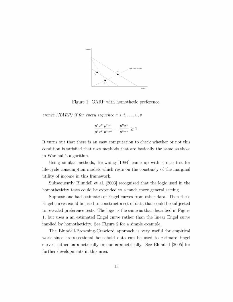
To get some intuition, consider Figure 1. The data (p1, x1) and (p2, x2) are

consistent with revealed preference. However, if the underlying preferences

are homothetic, then x3 would be demanded at the budget set p3, creating a

violation of revealed preference.

In general, the necessary and sufficient condition for an observed set of

choices to be consistent with homotheticity is given by HARP:

Definition 6 (Homothetic Axiom of Revealed Preference.) A set of

data (pt, xt) for t = 1, . . . , T satisfy the Homothetic Axiom of Revealed Pref-

12

GOOD 1

G OOD 2

Engel curve (linear)

x

x 1

x 3

2

Figure 1: GARP with homothetic preference.

erence (HARP) if for every sequence r, s, t, . . . , u, v

prxs

prxr

psxt

psxs· · ·

puxv

puxu≥ 1.

It turns out that there is an easy computation to check whether or not this

condition is satisfied that uses methods that are basically the same as those

in Warshall’s algorithm.

Using similar methods, Browning [1984] came up with a nice test for

life-cycle consumption models which rests on the constancy of the marginal

utility of income in this framework.

Subsequently Blundell et al. [2003] recognized that the logic used in the

homotheticity tests could be extended to a much more general setting.

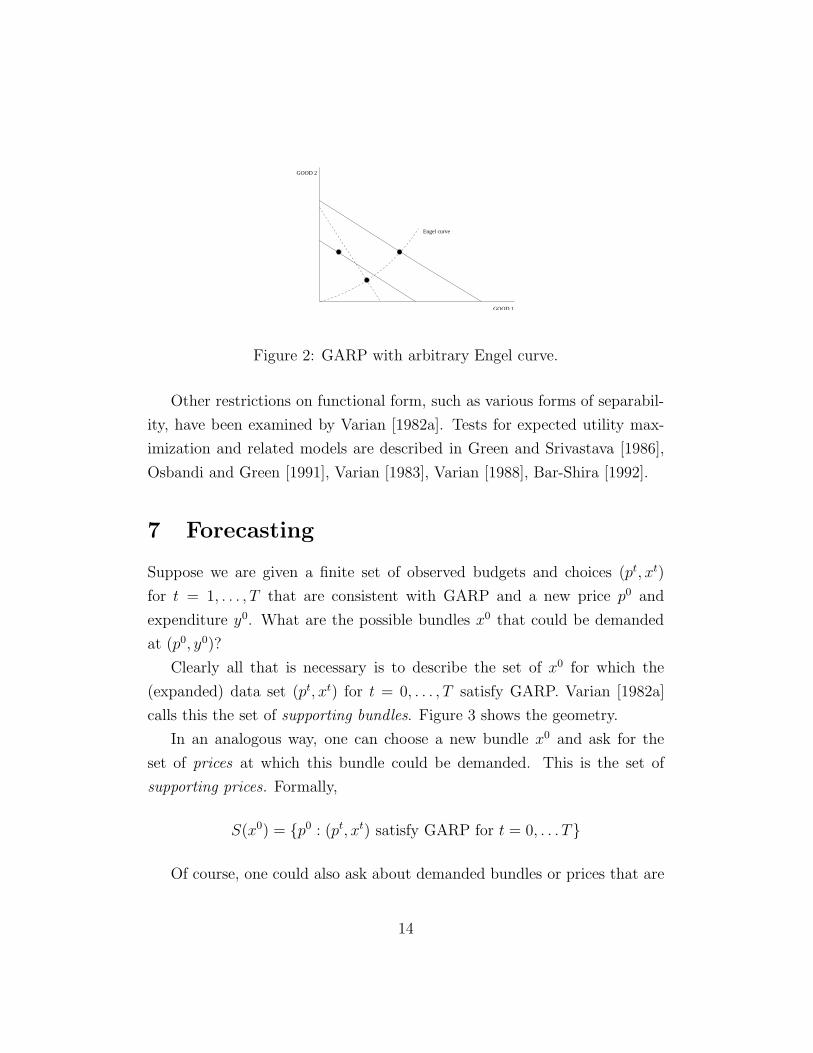
Suppose one had estimates of Engel curves from other data. Then these

Engel curves could be used to construct a set of data that could be subjected

to revealed preference tests. The logic is the same as that described in Figure

1, but uses a an estimated Engel curve rather than the linear Engel curve

implied by homotheticity. See Figure 2 for a simple example.

The Blundell-Browning-Crawford approach is very useful for empirical

work since cross-sectional household data can be used to estimate Engel

curves, either parametrically or nonparametrically. See Blundell [2005] for

further developments in this area.

13

GOOD 1

GOOD 2

Engel curve

Figure 2: GARP with arbitrary Engel curve.

Other restrictions on functional form, such as various forms of separabil-

ity, have been examined by Varian [1982a]. Tests for expected utility max-

imization and related models are described in Green and Srivastava [1986],

Osbandi and Green [1991], Varian [1983], Varian [1988], Bar-Shira [1992].

7 Forecasting

Suppose we are given a finite set of observed budgets and choices (pt, xt)

for t = 1, . . . , T that are consistent with GARP and a new price p0 and

expenditure y0. What are the possible bundles x0 that could be demanded

at (p0, y0)?

Clearly all that is necessary is to describe the set of x0 for which the

(expanded) data set (pt, xt) for t = 0, . . . , T satisfy GARP. Varian [1982a]

calls this the set of supporting bundles. Figure 3 shows the geometry.

In an analogous way, one can choose a new bundle x0 and ask for the

set of prices at which this bundle could be demanded. This is the set of

supporting prices. Formally,

S(x0) = {p0 : (pt, xt) satisfy GARP for t = 0, . . . T}

Of course, one could also ask about demanded bundles or prices that are

14

x2

x1

S(p0,y0)

(p0,y0)

Figure 3: Supporting bundles.

consistent with utility functions with various restrictions imposed such as

homotheticity, separability, specific forms for Engel curves and so on.

8 Recoverability

As we have seen, Afriat’s methods can be used to construct a utility func-

tion that is consistent with finite set of observed choices that satisfy GARP.

However, this is only one utility function. Typically there will be many other

such functions. Is there a way to describe the entire set of utility functions

(or preferences) consistent with some data?

Varian [1982a] posed the question in the following way. Suppose we are

given a finite set of data (pt, xt) for t = 2, . . . T that satisfies GARP and two

new bundles x0 and x1. Consider the set of prices at which which x0 could

be demanded, i.e., the supporting set of prices. If every such supporting

set makes x0 revealed preferred to x1 then we conclude that all preferences

consistent with the data must have x0 preferred to x1.

Given any x0, it is possible to define the sets of x’s that are revealed

15

x2

x1

P1

x1

x0

RP(x0)

RW(x0)

Figure 4: RP (x0) and RW (x0): simple case.

preferred to x0 (RP (x0)) and set of x’s that are revealed worse than x0

(RW (x0). A very simple example is shown in Figure 4. The possible set

of supporting prices for x0 must lie in the shaded cone so every such set of

prices imply that x0 is revealed preferred to the points in RW (x0). Similarly,

the points in the convex hull of the bundles revealed preferred to x0 must

themselves be preferred to x0 for any concave utility function that rationalizes

the data.

Of course Figure 4 uses only one observation. As we get more observations

on demand, we will get tighter bounds on RP (x0) and RW (x0), as shown in

Figure 5.

Another approach, also suggested by Varian [1982a] is to try to compute

bounds on specific utility functions. A very convenient choice in this case is

what Samuelson [1974] calls the money metric utility function. First define

the expenditure function

e(p, u) = min pz such that u(z) ≥ u.

16

x 2

x 1

RP(x 0 )

RW( x 0 )

x o

x 1

x 2

x 3

x 4

x 5

Figure 5: RP (x0) and RW (x0): a more complex case.

It is not hard to see that under minimal regularity conditions e(p, u) will be

a strictly increasing function of u. Now define

m(p, x) = e(p, u(x)).

For fixed p, m(p, x) is a strictly increasing function of utility, so it is itself a

utility function that represents the same preferences.

Varian [1982a] suggested that given a finite set of data (pt, xt) one could

define an upper bound to the money metric utility by using

m+(p, x) = min pzt such that ztRx.

Subsequently, Knoblauch [1992] showed that this bound was in fact tight:

there were preferences that rationalized the observed choices that had m+(p, x)

as their money-metric utility function. Varian [1982a] defined a lower bound

to Samuelson’s money metric utility function and showed that it was tight.

Of course, using restrictions on utility form such as HARP allow for

tighter bounds. There are several papers on the implications of such re-

17

strictions in the theory and measurement of index numbers, including Afriat

[1981], Afriat [1981], Diewert and Parkan [1985], Dowrick and Quiggin [1994],

Dowrick and Quiggin [1997], and Manser and McDonald [1988].

9 Summary

Samuelson’s 1938 theory of revealed preference has turned out to be amaz-

ingly rich. Note only does the Strong Axiom of Revealed Preference provide

a necessary and sufficient condition for observed choices to be consistent

with utility maximization, it also provides a very useful tool for empirical,

nonparametric analysis of consumer choices.

Up until recently, the major applications of Samuelson’s theory of revealed

preference have been in economic theory. As we get larger and richer sets of

data describing consumer behavior, nonparametric techniques using revealed

preference analysis will become more feasible. We anticipate that in the

future, revealed preference analysis will make a significant contribution to

empirical economics as well.

18

References

S. N. Afriat. The equivalence in two dimensions of the strong and weak

axioms of revealed preference. Metroeconomica, 17:24–28, 1965.

Sydney Afriat. The construction of a utility function from expenditure data.

International Economic Review, 8:67–77, 1967.

Sydney Afriat. On the constructibility of consistent price indices between

several periods simultaneously. In Angus Deaton, editor, Essays in Theory

and Measurement of Demand: in Honour of Sir Richard Stone. Cambridge

University Press, Cambridge, England, 1981.

Sydney Afriat. Logic of Choice and Economic Theory. Clarendon Press,

Oxford, 1987.

James Andreoni and John Miller. Giving according to GARP: An experi-

mental test of the consistency of preferences for altruism. Econometrica,

70(2):737–753, 2002.

Ziv Bar-Shira. Nonparametric test of the expected utility hypothesis. Amer-

ican Journal of Agricultural Economics, 74(3):523–533, 1992.

Raymond C. Battalio, John H. Kagel, Robin C. Winkler, Edwin B. Fisher,

Robert L BAsmann, and Leonard Krasner. A test of csnsumer demand

theory using observations of individual consumer purchases. Western Eco-

nomic Journal, 11(4):411–428, 1873.

Gary Becker. Irrational behavior and economic theory. Journal of Political

Economy, 70:1–13, 1962.

Richard Blundell. How revealing is revealed preference? European Economic

Journal, 3:211–235, 2005.

19

Richard Blundell, Martin Browning, and I. Crawford. Nonparametric Engel

curves and revealed preference. Econometrica, 71(1):205–240, 2003.

Stephen Bronars. The power of nonparametric tests. Econometrica, 55(3):

693–698, 1985.

Martin Browning. A non-parametric test of the life-cycle rational expecta-

tions hypothesis. International Economic Review, 30:979–992, 1984.

J. S. Chipman, L. Hurwicz, M. K. Richter, and H. F. Sonnenschein. Prefer-

ences, Utility and Demand. Harcourt Brace Janovich, New York, 1971.

Dale Christensen, Lars, Jorgensen and Lawrence Lau. Transcendental loga-

rithmic utility functions. American Economic Review, 65:367–383, 1975.

James C. Cox. On testing the utility hypothesis. Technical report, University

of Arizona, 1989.

Angus Deaton. Demand analysis. In Z. Griliches and M. Intrilligator, editors,

Handbook of Econometrics. JAI Press, Greenwich, CT, 1983.

Erwin Diewert and Celick Parkan. Tests for consistency of consumer data

and nonparametric index numbers. Journal of Econometrics, 30:127–147,

1985.

W. E. Diewert. Afriat and revealed preference theory. The Review of Eco-

nomic Studies, 40(3):419–425, 1973.

A. R. Dobell. A comment on A. Y. C. Koo’s an empirical test of revealed

preference theory. Econometrica, 33(2):451–455, 1965.

Steve Dowrick and John Quiggin. International comparisons of living stan-

dards and tastes: A revealed-preference analysis. The American Economic

Review, 84(1):332–341, 1994.

20

Steve Dowrick and John Quiggin. True measures of GDP and convergence.

The American Economic Review, 87(1):41–64, 1997.

M. Famulari. A household-based, nonparametric test of demand theory. Re-

view of Economics and Statistics, 77:372–383, 1995.

Richard Green and Sanjay Srivastava. Expected utility maximization and

demand behavior. Journal of Economic Theory, 38(2):313–323, 1986.

John Gross. Testing data for consistency with revealed preference. The

Review of Economics and Statistics, 77(4):701–710, 1995.

William T. Harbaugh, Kate Krause, and Timoth R. Berry. GARP for kids:

on the development of rational choice theory. American Economic Review,

91(5):1539–1545, 2001.

J. R. Hicks. Value and Capital. Oxford University Press, Oxford, England,

1939.

H. S. Houthakker. Revealed preference and the utility function. Economica,

17(66):159–174, 1950.

M. Houtman and J. A. Maks. Determining all maximial data subsets consis-

tent with revealed preference. Kwantitatieve Methoden, 19:89–104, 1985.

John H. Kagel, Raymond C. Battalio, and Leonard Green. Choice The-

ory: An Experimental Analysis of Animal Behavior. Cambridge University

Press, Cambridge, England, 1995.

Vicki Knoblauch. A tight upper bound on the money metric utility function.

The American Economic Review, 82(3):660–663, 1992.

Anthony Y. C. Koo. An empirical test of revealed preference theory. Econo-

metrica, 31(4):646–664, 1963.

21

Anthony Y. C. Koo. A comment on A. Y. C. Koo’s an empirical test of

revealed preference theory: Reply. Econometrica, 33(2):456–458, 1965.

I. M. D. Little. A reformulation of the theory of consumers’ behavior. Oxford

Economic Papers, 1:90–99, 1949.

Marilyn Manser and R. McDonald. An analysis of substitution bias in mea-

suring inflation, 1959–85. Econometrica, 56:909–930, 1988.

Peter Newman. Complete ordering and revealed preference. Economica, 27:

65–77, 1960.

Kent Osbandi and Edward J. Green. A revealed preference theory for ex-

pected utility. The Review of Economic Studies, 58(4):677–695, 1991.

Marcel K. Richter. Revealed preference theory. Econometrica, 34(3):635–645,

1966.

H. Rose. Consistency of preference: The two-commodity case. Review of

Economic Studies, 25:124–125, 1958.

Paul A. Samuelson. A note on the pure theory of consumer’s behavior.

Economica, 5(17):61–71, 1938.

Paul A. Samuelson. Consumption theory in terms of revealed preference.

Economica, 15(60):243–253, 1948.

Paul A. Samuelson. The problem of integrability in utility theory. Economica,

17(68):355–385, 1950.

Paul A. Samuelson. Consumption theorems in terms of overcompensation

rather than indifference comparisons. Economics, 20(77):1–9, 1953.

Paul A. Samuelson. Complementarity: an essay on the 40th anniversary

of the Hicks-Allen revolution in demand theory. Journal of Economic

Literature, 12(4):1255–1289, 1974.

22

Dieter Sondermann. Revealed preference: An elementary treatment. Econo-

metrica, 50(3):777–780, 1982.

Bernt P. Stigum. Revealed preference–A proof of Houthakker’s theorem.

Econometrica: Journal of the Econometric Society, 41(3):411–423, 1973.

H. Uzawa. Preference and rational choice in the theory of consumption. In

K. J. Arrow, S. Karlin, and P. Suppes, editors, Mathematical Models in

Social Science. Stanford University Press, Stanford, CA, 1960.

Hal R. Varian. The nonparametric approach to demand analysis. Economet-

rica, 50(4):945–972, 1982a.

Hal R. Varian. Nonparametric test of models of consumer behavior. Review

of Economic Studies, 50:99–110, 1982b.

Hal R. Varian. Nonparametric tests of models of investor behavior. Journal

of Financial and Quantitative Analysis, 18(3):269–278, 1983.

Hal R. Varian. Estimating risk aversion from Arrow-Debreu portfolio choice.

Econometrica, 56(4):973–979, 1988.

Hal R. Varian. Goodness-of-fit in optimizing models. Journal of Economet-

rics, 46:125–140, 1990.

S. Warshall. A theorem on Boolean matrices. Journal of the Association of

Computing Machinery, 9:11–12, 1962.

Gerald A. Whitney and James L. Swofford. Nonparametric tests of utility

maximization and weak separability for consumption, leisure and money.

The Review of Economic Statistics, 69(3):458–464, 1987.

T. Yokoyama. A logical foundation of the theory of consumer’s demand. In

P. Newman, editor, Readings in Mathematical Economics. Johns Hopkins

Press, Baltimore, 1968.

23