2000- balancing static and dynamic testing: some ... · (an exercise for the reader). v. 1.2,...
TRANSCRIPT
Title Slide
2000-
"Balancing static and dynamic testing:Some observations from measurement"
by
Les Hatton
Oakwood Computing, Surrey, U.K. andthe Computing Laboratory, University of Kent
Version 1.2: 09/Mar/2000
©Copyright, L.Hatton, 2000-
OAKWOOD COMPUTING - SURVIVAL AND AVOIDANCE STRATEGIES FOR SOFTWARE FAILURE. . . . . . . . . . . . . . . . . . . . . . . . . . . . . . . . . . . . . . . . . . . . . . . . . . . . . . . . . . . . . . . . . . . . . . . . . . . . . . . . . . .

v. 1.2, 09/Mar/2000 , (slide 1 - 2). Not to be copied without permission from copyright holder. © L.Hatton, 2000-
Overview
v Static v. dynamic testingv Forensic work: patterns in failurev Wallowing in data

v. 1.2, 09/Mar/2000 , (slide 1 - 3). Not to be copied without permission from copyright holder. © L.Hatton, 2000-
Control Process feedback - the essence of engineering improvement
Process Product
Measure samples of product for
quality
Feed-back into Process to improve it
If you want to improve reliability, measure andanalyse failures.

v. 1.2, 09/Mar/2000 , (slide 1 - 4). Not to be copied without permission from copyright holder. © L.Hatton, 2000-
Preparing the ground
Fixing the definitions– A fault is a statically detectable property
of a piece of code or a design– A failure is a fault or set of faults which
together cause the system to show unexpected behaviour at run-time
– A defect or bug is a generic term for either faults which fail or faults which do not.
– Fault density is the number of faults divided by the number of lines of code

v. 1.2, 09/Mar/2000 , (slide 1 - 5). Not to be copied without permission from copyright holder. © L.Hatton, 2000-
Preparing the ground
Note that the causal relationship between fault and failure differs in some standards:-
• IEEE + other sources:error -> fault -> failure
• IEC 61508, (formerly IEC SC 65A):fault -> error -> failure

v. 1.2, 09/Mar/2000 , (slide 1 - 6). Not to be copied without permission from copyright holder. © L.Hatton, 2000-
Preparing the ground
The basis of measurement is to define the dependent and independent variables– Independent variables
u LOC (line of code)u Timeu Function points
– Dependent variablesu Defect typeu Defect severity

v. 1.2, 09/Mar/2000 , (slide 1 - 7). Not to be copied without permission from copyright holder. © L.Hatton, 2000-
What is a line of code ?
Correlation between two measures of source lines in C
0
50000
100000
150000
200000
250000
300000
0 100000 200000 300000 400000 500000
Total pre-processed lines
Correlation between two measures of line of codein systems written in C. The two measures areexecutable lines and total number of pre-processedlines, Hatton (1995).

v. 1.2, 09/Mar/2000 , (slide 1 - 8). Not to be copied without permission from copyright holder. © L.Hatton, 2000-
Fault density is a function of time
Faultsper1000lines
DKLOC
Time of testing
Fault density depends on how much the system has been used, (c.f. HP)

v. 1.2, 09/Mar/2000 , (slide 1 - 9). Not to be copied without permission from copyright holder. © L.Hatton, 2000-
Where and how do defects occur historically ?
All faults
Those faultswhich fail
v. 1.2, 09/Mar/2000 , (slide 1 - 10). Not to be copied without permission from copyright holder. © L.Hatton, 2000-
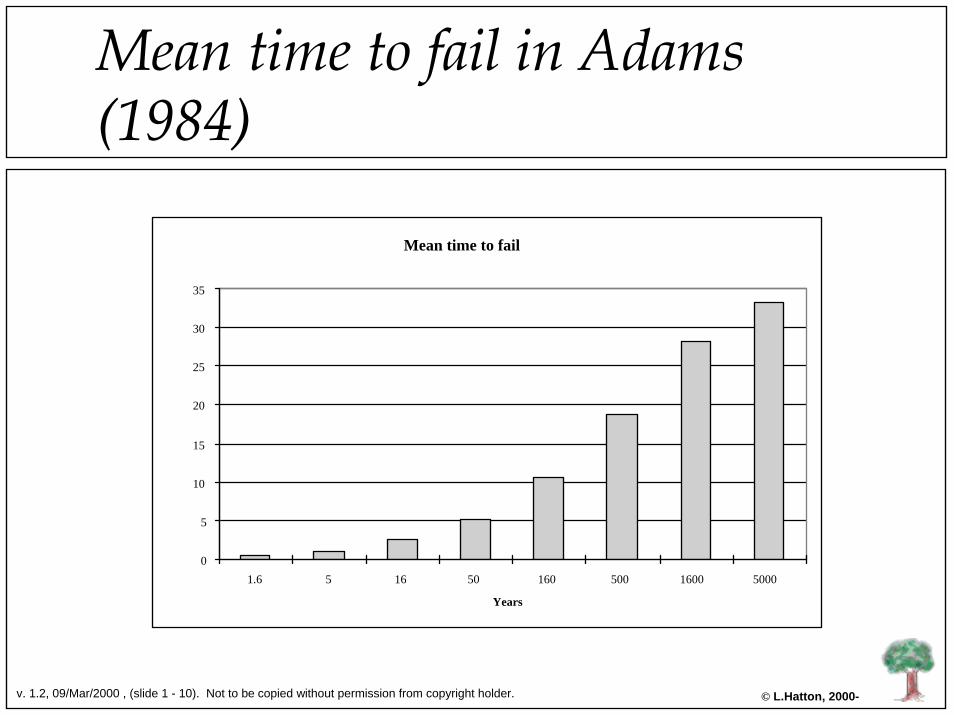
Mean time to fail in Adams (1984)
Mean time to fail
0
5
10
15
20
25
30
35
1.6 5 16 50 160 500 1600 5000
Years

v. 1.2, 09/Mar/2000 , (slide 1 - 11). Not to be copied without permission from copyright holder. © L.Hatton, 2000-
Cost v. detection point
Cost of fixing defects
0
10
20
30
40
50
60
70
80
90
100
Req
uire
men
ts D
esig
n
Cod
ing
Uni
t tes
ting
Acc
epta
nce
test
ing
Ope
ratio
n
LowHigh
Embedded systems tend to follow the high curve.Data from Boehm, (1981) and many others.Note that curve kicks only around coding stage.

v. 1.2, 09/Mar/2000 , (slide 1 - 12). Not to be copied without permission from copyright holder. © L.Hatton, 2000-
Overview
v Static v. dynamic testingv Forensic work: patterns in failurev Wallowing in data

v. 1.2, 09/Mar/2000 , (slide 1 - 13). Not to be copied without permission from copyright holder. © L.Hatton, 2000-
Patterns in failure
There are two complicating factors in the forensic analysis of software failure
• Exponentially increasing complexity• Chaotic behaviour

v. 1.2, 09/Mar/2000 , (slide 1 - 14). Not to be copied without permission from copyright holder. © L.Hatton, 2000-
Exponentially increasing complexity
The amount of software in consumer electronic products is currently doubling about every 18 months.
• Line-scan TVs have ~250,000 lines of C.• There are around 200,000 lines of C in a car.• Most consumer devices, washing-machines
and so on have a few K of software.• The Airbus A340 and Boeing 777 are totally
dependent on software.

v. 1.2, 09/Mar/2000 , (slide 1 - 15). Not to be copied without permission from copyright holder. © L.Hatton, 2000-
Chaotic behaviour
AT & T Jan, Jan 15, 1990:• Single misplaced line of C in 3 million lines by-
passed network error-recovery code• For 9 hours, millions of long-distance callers
just heard message “all circuits are busy”• Reported $1.1 billion loss

v. 1.2, 09/Mar/2000 , (slide 1 - 16). Not to be copied without permission from copyright holder. © L.Hatton, 2000-
Anatomy of a $1billion bug
...switch( message ){case INCOMING_MESSAGE:
if ( sending_switch == OUT_OF_SERVICE ){
if ( ring_write_buffer == EMPTY )send_in_service_to_smm(3B);
elsebreak; /* Whoops ! */
}process_incoming_message(); /* skipped */break;
...}do_optional_database_work();...

v. 1.2, 09/Mar/2000 , (slide 1 - 17). Not to be copied without permission from copyright holder. © L.Hatton, 2000-
Chaotic behaviour
Cars too ...:• 22/July/1999. General Motors has to recall 3.5
million vehicles because of a software defect. Stopping distances were extended by 15-20 metres.
• Federal investigators received almost 11,000 complaints as well reports of 2,111 crashes and 293 injuries.
• Recall costs ? (An exercise for the reader).

v. 1.2, 09/Mar/2000 , (slide 1 - 18). Not to be copied without permission from copyright holder. © L.Hatton, 2000-
The PC picture ...
0.1
1
10
100
1000
10000
W'95 Macintosh7.5-8.1
NT 4.0 Linux Sparc4.1.3c
OS
Mean Time Between Failures of various operating systems

v. 1.2, 09/Mar/2000 , (slide 1 - 19). Not to be copied without permission from copyright holder. © L.Hatton, 2000-
Useful links
v On software failure:-– http://www.csl.sri.com/risks.html, (general failures)– http://www.rvs.uni-bielefeld.de/publications,
(aircraft)– http://www.bugnet.com/, (PC)– http://www.oakcomp.co.uk/TechPub.html, (general
failure)

v. 1.2, 09/Mar/2000 , (slide 1 - 20). Not to be copied without permission from copyright holder. © L.Hatton, 2000-
Overview
v Static v. dynamic testingv Forensic work: patterns in failurev Wallowing in data

v. 1.2, 09/Mar/2000 , (slide 1 - 21). Not to be copied without permission from copyright holder. © L.Hatton, 2000-
Where and how do defects occur historically ?
Looking for properties of defects– Defects tend to cluster, (in one case 47% of
defects in 4% of modules in IBM’s S/370 OS– The earlier you find them, the cheaper you
find them

v. 1.2, 09/Mar/2000 , (slide 1 - 22). Not to be copied without permission from copyright holder. © L.Hatton, 2000-
Where and how do defects occur historically ?
Where you find one, you find more, (Pfleeger, (1998))
Defect clustering
0
10
20
30
40
50
60
70
80
90
C2 C J G
G2 N T
C3 W D F
C1 O
W1
D1 P
G1 L S U Z
Oth
ers
Component

v. 1.2, 09/Mar/2000 , (slide 1 - 23). Not to be copied without permission from copyright holder. © L.Hatton, 2000-
Where and how do defects occur historically ?
Defect density clustering
0
2
4
6
8
10
12
14
16
18
20
C2
C3 P C L
G2 N J G F W G1 S D O
W1
C4 M D1 I Z B
Component
Where you find one, you find more.The effect is even more emphatic when you normaliseagainst lines of code. (Hatton (1998), Pfleeger, (1998))

v. 1.2, 09/Mar/2000 , (slide 1 - 24). Not to be copied without permission from copyright holder. © L.Hatton, 2000-
Where and how do defects occur historically ?
The following slides show distributions of faults and failures from a number of case studies, each with an introduction and a conclusion.
v. 1.2, 09/Mar/2000 , (slide 1 - 25). Not to be copied without permission from copyright holder. © L.Hatton, 2000-
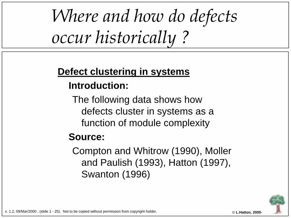
Where and how do defects occur historically ?
Defect clustering in systemsIntroduction:The following data shows how
defects cluster in systems as a function of module complexity
Source:Compton and Whitrow (1990), Moller
and Paulish (1993), Hatton (1997), Swanton (1996)

v. 1.2, 09/Mar/2000 , (slide 1 - 26). Not to be copied without permission from copyright holder. © L.Hatton, 2000-
Failures and component size, (new and changed)
Size in statements
0
1
2
3
4
5
6
7
8
9
10 30 50 70 90 110
Moller new actual
Moller new pred
Moller chg actual
Moller chg pred
Data from an OS study at Siemens (1993)

v. 1.2, 09/Mar/2000 , (slide 1 - 27). Not to be copied without permission from copyright holder. © L.Hatton, 2000-
What happens for big components ?
Logarithmic Quadratic
Average size in statements
0
2
4
6
8
10
12
14
16
18
60
100
160
250
400
630
1000
2000
C&W Ada
Moller Columbus
Prediction

v. 1.2, 09/Mar/2000 , (slide 1 - 28). Not to be copied without permission from copyright holder. © L.Hatton, 2000-
Failure density and component size
Average size in statements
0
2
4
6
8
10
1260
100
160
250
400
630
1000
2000
C&W density data
Moller Columbus
Comparison of Ada and assembler,Hatton (1997)

v. 1.2, 09/Mar/2000 , (slide 1 - 29). Not to be copied without permission from copyright holder. © L.Hatton, 2000-
Failure density and component size
Defect density v. C function size
0
10
20
30
40
50
60
70
0-20 20-40 40-80 80-160 160-320 > 320
function size in lines
Data from the GNU indent program, Swanton (1996)
v. 1.2, 09/Mar/2000 , (slide 1 - 30). Not to be copied without permission from copyright holder. © L.Hatton, 2000-
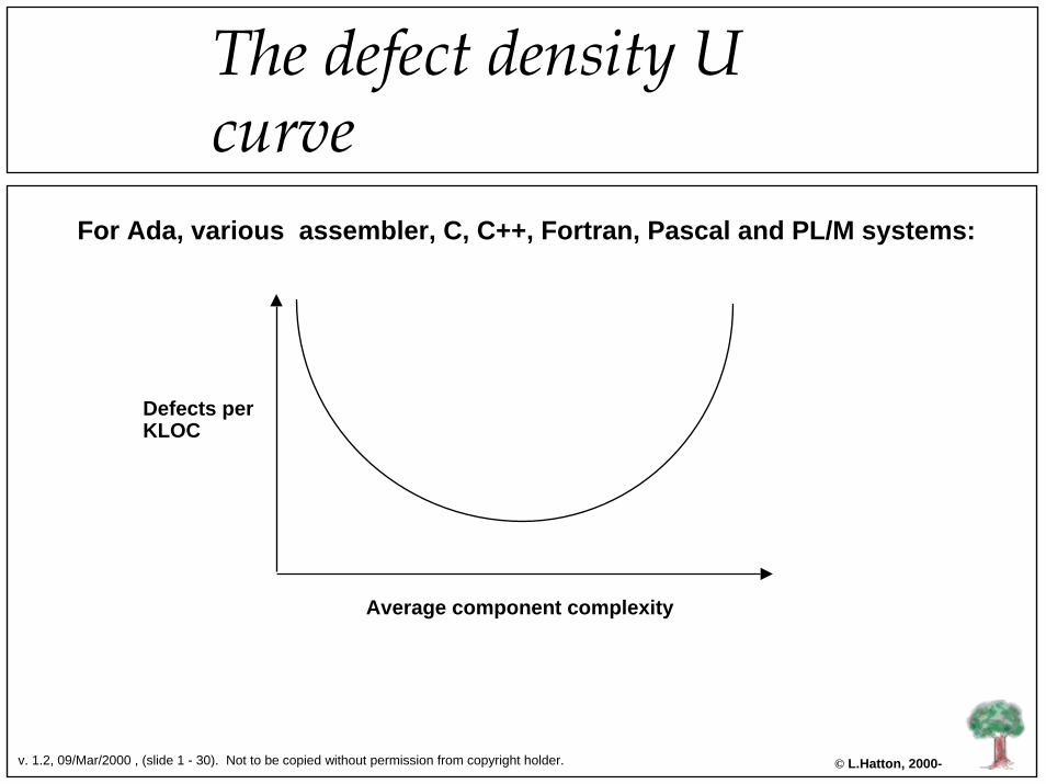
The defect density U curve
For Ada, various assembler, C, C++, Fortran, Pascal and PL/M systems:
Defects perKLOC
Average component complexity
v. 1.2, 09/Mar/2000 , (slide 1 - 31). Not to be copied without permission from copyright holder. © L.Hatton, 2000-
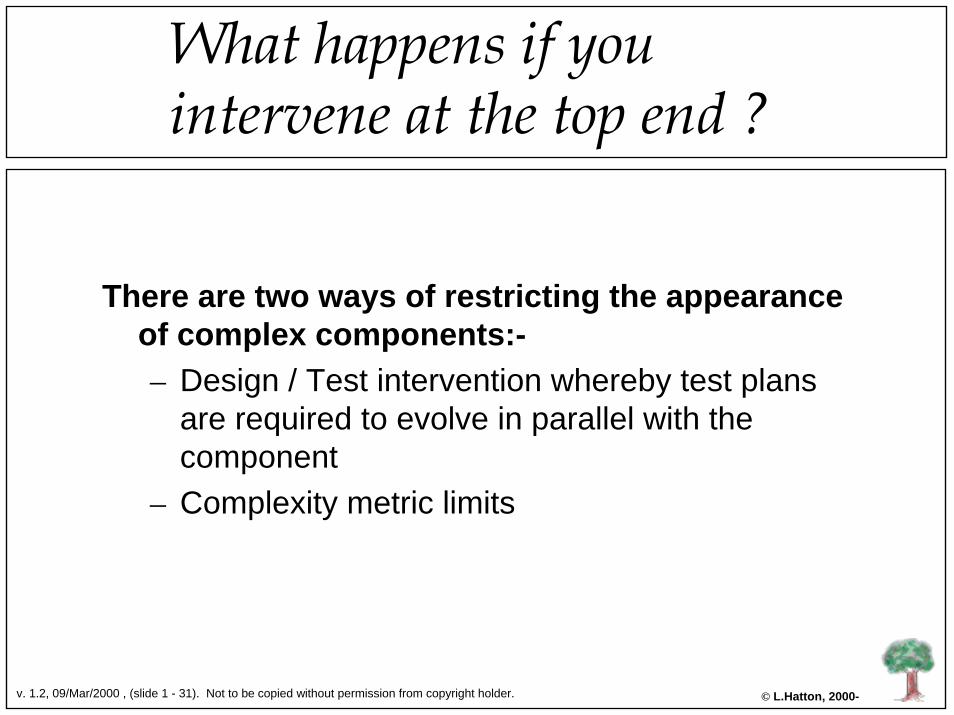
What happens if you intervene at the top end ?
There are two ways of restricting the appearance of complex components:-– Design / Test intervention whereby test plans
are required to evolve in parallel with the component
– Complexity metric limits

v. 1.2, 09/Mar/2000 , (slide 1 - 32). Not to be copied without permission from copyright holder. © L.Hatton, 2000-
Complexity measurement limiting
Complexity testing generally includes the following:-– Measurement of complexity values such as
lines of code (LOC), cyclomatic or path complexity
– Identification of the worst 10% of a population– Using the known properties of the U curve to
exclude this 10%

v. 1.2, 09/Mar/2000 , (slide 1 - 33). Not to be copied without permission from copyright holder. © L.Hatton, 2000-
The defect density U curve -invasive truncation
In those systems where excessive complexity has been restricted:-
Defects perKLOC
Average component complexity

v. 1.2, 09/Mar/2000 , (slide 1 - 34). Not to be copied without permission from copyright holder. © L.Hatton, 2000-
Complexity measurement limiting
Complexity measures:-– Cyclomatic complexity is a count of the number
of decisions plus 1, (in an if else, don’t count the else. In a switch, don’t count the default).
– The path count is calculated by assuming that every decision is independent. Sequential blocks multiply and parallel blocks add.

v. 1.2, 09/Mar/2000 , (slide 1 - 35). Not to be copied without permission from copyright holder. © L.Hatton, 2000-
Cyclomatic complexity distributions
0
1
2
3
4
5
6
7
8
90-1
00
80-9
0
70-8
0
60-7
0
50-6
0
40-5
0
30-4
0
20-3
0
10-2
0
0-10
Percentiles
UnrestrictedRestricted
Note the effectiveness of complexity limiting here (lower curve)in excluding the dangerous upper end in this experiment
Complexity measurement limiting

v. 1.2, 09/Mar/2000 , (slide 1 - 36). Not to be copied without permission from copyright holder. © L.Hatton, 2000-
Path complexity distributions
0
1
2
3
4
5
6
90-1
00
80-9
0
70-8
0
60-7
0
50-6
0
40-5
0
30-4
0
20-3
0
10-2
0
0-10
Percentiles
UnrestrictedRestricted
The same complexity limiting is equally successful at controllingpath complexity, improving dynamic testability dramatically.
Complexity measurement limiting

v. 1.2, 09/Mar/2000 , (slide 1 - 37). Not to be copied without permission from copyright holder. © L.Hatton, 2000-
Complexity measurement limiting
Complexity limiting notes:-– It doesn’t seem to matter which complexity
metric you use to do this, they are currently very crude
– It should be used at either end because of the U-curve effect.

v. 1.2, 09/Mar/2000 , (slide 1 - 38). Not to be copied without permission from copyright holder. © L.Hatton, 2000-
Where and how do defects occur historically ?
Defect clustering in systemsDefects are not spread equally as a function of component size. They tend to cluster
Conclusion:– Use defect clustering to guide
inspection and testing strategies– Use complexity metric limits

v. 1.2, 09/Mar/2000 , (slide 1 - 39). Not to be copied without permission from copyright holder. © L.Hatton, 2000-
Where and how do defects occur historically ?
Statically detectable faultIntroduction:The following slides show the distribution of
statically detectable inconsistencies and widely-known faults in C and Fortran 77
These were measured using purpose built tools exploiting the knowledge base of such behaviour
Source:Hatton (1995)
v. 1.2, 09/Mar/2000 , (slide 1 - 40). Not to be copied without permission from copyright holder. © L.Hatton, 2000-
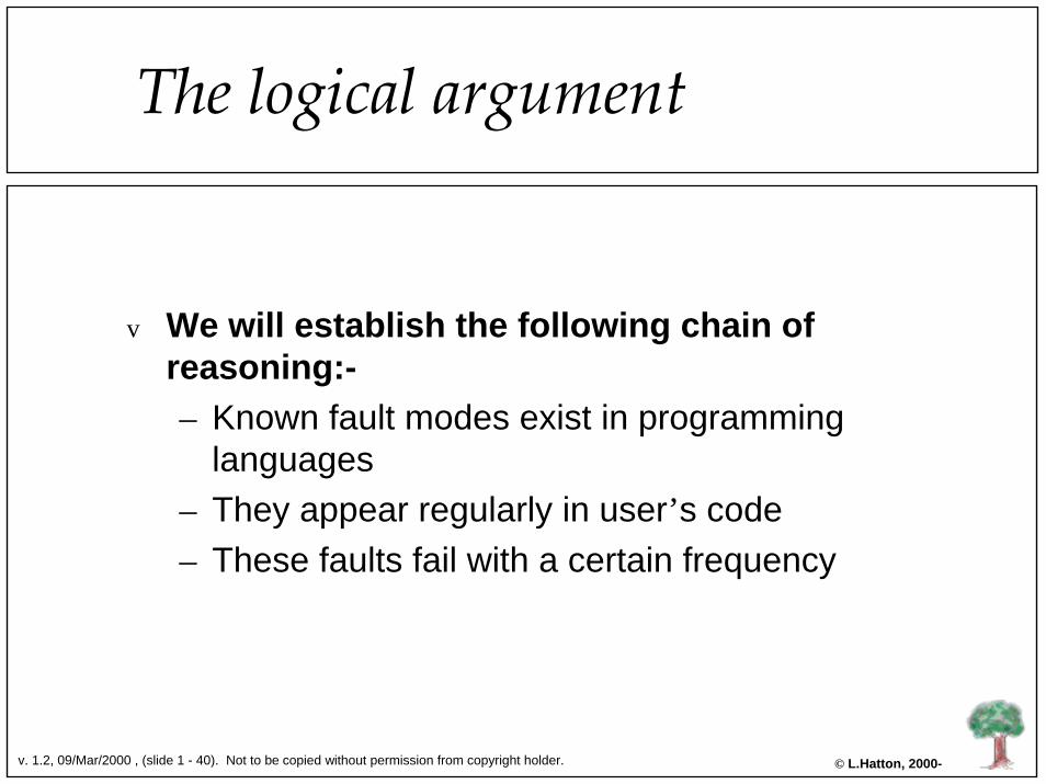
The logical argument
v We will establish the following chain of reasoning:-– Known fault modes exist in programming
languages– They appear regularly in user’s code– These faults fail with a certain frequency

v. 1.2, 09/Mar/2000 , (slide 1 - 41). Not to be copied without permission from copyright holder. © L.Hatton, 2000-
Sources of information
v Sources of information on problematic behaviour in languages come from two sources:-– The committee’s work, (formally identified
problem areas). Approximately 300 items.– Experience in the world at large through news
groups, comp.lang.c, the Obfuscated C competition and so on, (informally identified problem areas). Approximately 400 items.
v. 1.2, 09/Mar/2000 , (slide 1 - 42). Not to be copied without permission from copyright holder. © L.Hatton, 2000-
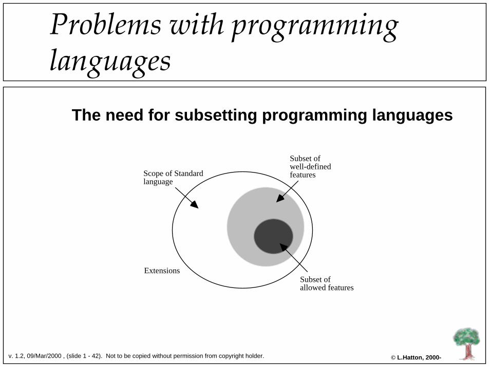
Problems with programming languages
The need for subsetting programming languages
Scope of Standard language
Subset of well-defined features
ExtensionsSubset of allowed features

v. 1.2, 09/Mar/2000 , (slide 1 - 43). Not to be copied without permission from copyright holder. © L.Hatton, 2000-
Formally identified problem areas
v Let us consider C. The following areas of C are problematic:– At standardisation in 1990 (197 items)
u Unspecified behaviouru Undefined behaviouru Implementation-defined behaviouru Locale-specific behaviour
– Since standardisation (119 items)u Defect Reports

v. 1.2, 09/Mar/2000 , (slide 1 - 44). Not to be copied without permission from copyright holder. © L.Hatton, 2000-
Examples reported by user community
v There are approximately 400 known. They are usually well-defined but misleading.Examples:– Returning the address of a local from a
function.– Assignment in a conditional
if ( a = b )
– Relational equality in an assignmenta == b;
– Spare semi-colons:if ( a == b ); { ... }

v. 1.2, 09/Mar/2000 , (slide 1 - 45). Not to be copied without permission from copyright holder. © L.Hatton, 2000-
Fault frequencies in C applications
Wei
ghte
d fa
ults
per
100
0 lin
es.
0
5
10
15
20
25G
raph
ics
Gen
eral
Elec
-eng
Des
ign
Syst
em
Con
trol
Dat
abas
e
Gra
phic
s
Pars
ing
Pars
ing
Insu
ranc
e
Util
ities
Util
ities
Util
ities
Con
trol
Com
ms
Com
ms
Averageof 8
Data like this is extractable using tools such as the Safer C Toolset,(http://www.oakcomp.co.uk)

v. 1.2, 09/Mar/2000 , (slide 1 - 46). Not to be copied without permission from copyright holder. © L.Hatton, 2000-
Fault frequencies in Fortran 77 applications
Wei
ghte
d fa
ults
per
100
0 lin
es.
0
5
10
15
20
25ge
nera
l
elc-
eng
Earth
Sci
pars
ing
Cad
Cam
Che
mM
od
Earth
Sci
elc-
eng
fld-e
ng
mch
-eng
mch
-eng
nuc-
eng
nuc-
eng
oper
-rs
Cad
Cam
the-
phys
Geo
desy
Aer
ospa
ce
gene
ral
Averageof 12
Same application areaone at 140 / KLOC and oneat 0 / KLOC

v. 1.2, 09/Mar/2000 , (slide 1 - 47). Not to be copied without permission from copyright holder. © L.Hatton, 2000-
Where and how do defects occur historically ?
Data derived from CAA CDIS
00.5
11.5
22.5
33.5
4
Averagedynamictesting
Thoroughdynamictesting
This study shows that statically detectable faults do in fact failduring the life-cycle of the software.

v. 1.2, 09/Mar/2000 , (slide 1 - 48). Not to be copied without permission from copyright holder. © L.Hatton, 2000-
Where and how do defects occur historically ?Conclusions on safer subsetting:– We can prove the following:
u There is a class of defect in programming languages which to a significant extent is statically detectable, widely reported and entirely avoidable
u This class of defect evades conventional testing to the extent of around 8 residual defects per 1000 lines of code
u A significant percentage of this class of defect fails during the life-cycle of the code but we are not able to predict which faults fail, so we must remove them all.
– Engineer education and tool support is crucial to the control of this class of defect.
v. 1.2, 09/Mar/2000 , (slide 1 - 49). Not to be copied without permission from copyright holder. © L.Hatton, 2000-
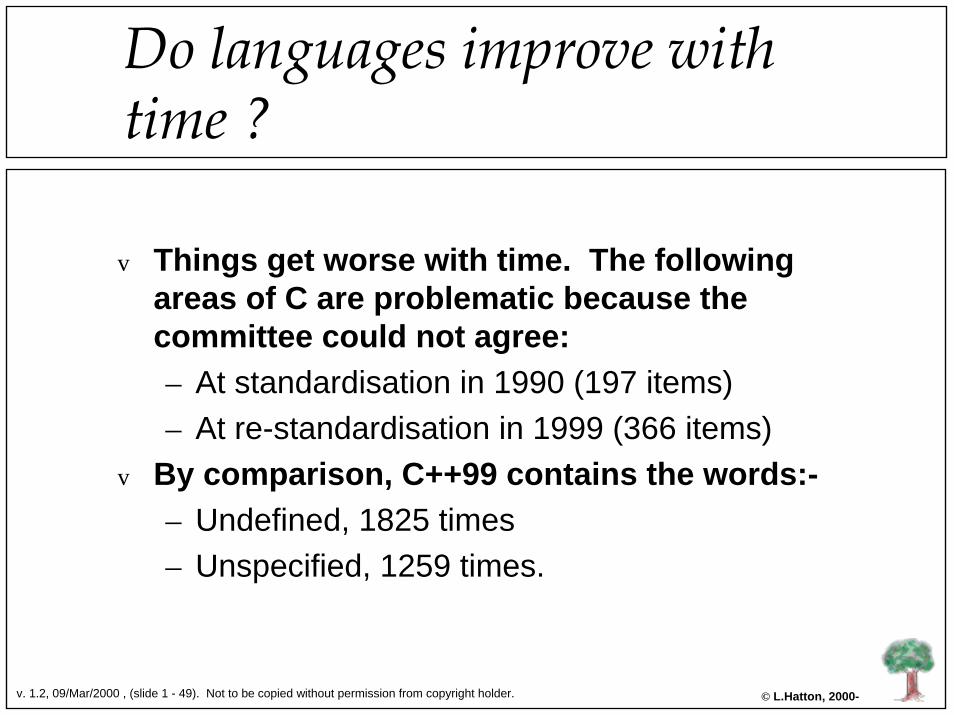
Do languages improve with time ?
v Things get worse with time. The following areas of C are problematic because the committee could not agree:– At standardisation in 1990 (197 items)– At re-standardisation in 1999 (366 items)
v By comparison, C++99 contains the words:-– Undefined, 1825 times– Unspecified, 1259 times.

v. 1.2, 09/Mar/2000 , (slide 1 - 50). Not to be copied without permission from copyright holder. © L.Hatton, 2000-
Why languages can’t improve
ADD NEWFEATURES
Re-standardise
language
Recognise poorfeatures
Feedbackcrippled bybackwards
compatibility
Using the model of control process feedback, we see thatthe feedback stage is crippled by the “shall not break oldcode” rule or “backwards compatibility” as it is morecommonly known.

v. 1.2, 09/Mar/2000 , (slide 1 - 51). Not to be copied without permission from copyright holder. © L.Hatton, 2000-
Where and how do defects occur historically ?
Statically detectable faultStatic analysis suffers from a noise problem
u When sometimes its a fault and sometimes not, for example:-
if ( a = b )instead ofif ( a == b )
u In this case, if we warn of all transgressions those statements which are OK will tend to hide those which are not from the programmer. The ‘signal’ is hidden by the noise.
u Some form of filtering is necessary, to maximise the likelihood of positive detection, for example a safer subset standard.

v. 1.2, 09/Mar/2000 , (slide 1 - 52). Not to be copied without permission from copyright holder. © L.Hatton, 2000-
Where and how do defects occur historically ?
Statically detectable faultWe do not know in advance which statically
detectable faults will fail, but on average a significant percentage will
Conclusions:– Source code should not be released with
any statically detectable fault– Learn about the fault modes of your
language– Beware of the static noise problem

v. 1.2, 09/Mar/2000 , (slide 1 - 53). Not to be copied without permission from copyright holder. © L.Hatton, 2000-
Conclusions
The view from data:-– Static testing v. dynamic testing
u Efficient static testing via inspections with semi-automated tool support has a dramatic beneficial effect on software reliability and production cost
– Tool supportu Automation should and can support:-
– The best static fault detection possible– Education of engineers on difficult language areas– Manual code inspections– Dynamic checking– Simple complexity control

v. 1.2, 09/Mar/2000 , (slide 1 - 54). Not to be copied without permission from copyright holder. © L.Hatton, 2000-
More information ...
For more information on safer subsets, static testing, downloadable technical publications and tools and other links, you are invited to browse our site:-
http://www.oakcomp.co.uk/

v. 1.2, 09/Mar/2000 , (slide 1 - 55). Not to be copied without permission from copyright holder. © L.Hatton, 2000-
Bibliography• Bach, R. (1997) “Test automation snake oil”, 14th annual conference on Testing Computer
Software, Washington, USA• Beizer, B. (1990). Software Testing Techniques. Van Nostrand Reinhold.• Brettschneider, (1989) “Is your software ready for release ?”, IEEE Software, July, p. 100-108• Fagan, M.E. (1976) “Design and code inspections to reduce errors in program development”, IBM
Systems Journal, 15(3), p. 182-211.• Fenton, N. E. (1991). Software Metrics: A Rigorous Approach. Chapman and Hall.• Genuchten, M. v. (1991). Towards a Software Factory. Eindhoven.• Gilb, T. & Graham D. (1993) Software Inspection, Addison-Wesley• Grady, R. B. and D. L. Caswell (1987). Software Metrics: Establishing a Company-Wide Program.
Englewood Cliffs, N.J., Prentice-Hall.• Graham, D. (1995) “A software inspection (failure) story”, EuroStar’95, London, November• Hatton, L. et. al. (1988). “SKS: an exercise in large-scale Fortran portability”, Software Practice
and Experience.• Hatton, L. (1995) “Safer C: Developing for High-Integrity and Safety-Critical Systems. McGraw-
Hill, ISBN 0-07-707640-0.• Hatton, L. (1997) Re-examining the fault density - component size connection, IEEE Software,
March-April 1997.• Hatton, L. (1997) The T experiments: errors in scientific software, IEEE Computational Science &
Engineering, vol 4, 2• Hatton, L. (1998) Does OO sync with the way we think ?, IEEE Software, May/June 1997• Hatton, L. (2000) “Software failure: avoiding the avoidable and living with the rest”, Addison-
Wesley, to appear in 2000.• Humphreys, W. (1995) “A discipline of software engineering”, Addison-Wesley, ISBN 0-201-
54610-8

v. 1.2, 09/Mar/2000 , (slide 1 - 56). Not to be copied without permission from copyright holder. © L.Hatton, 2000-
Bibliography
• IEC 61508 (1991). Software for computers in the application of industrial safety-related systems. International Electrotechnical Commission: Drafts only - cannot yet be referenced.
• Knight, J. C., A. G. Cass, et al. (1994). Testing a safety-critical application. International Symposium on Software Testing and Analysis (ISSTA'94), Seattle, ACM.
• Kolawa, A. (1999) “Mutation Testing: a new approach to automatic error detection”, StarEast ‘99,Orlando, May 1999
• Liedtke, C, and Ebert, H. (1995), “On the benefits of reinforcing code inspection activities”, EuroStar’95, London
• Leveson, N. (1995). “Safeware: System Safety and Computers.” Addison-Wesley, ISBN 0-201-11972-2.
• Littlewood, B. and L. Strigini (1992). “Validation of Ultra-High Dependability for Software-based Systems.” Comm ACM to be published:
• McCabe, T. A. (1976). “A complexity measure.” IEEE Trans Soft. Eng. SE-2(4): 308-320.• Mills, H.D. (1972) “On the statistical validation of computer programs”, IBM Federal Systems
Division. Gaithersburg, MD, Red. 72-6015, 1972• Myers, G. J. (1979). The Art of Software Testing. New York, John Wiley & Sons.• Nejmeh, B. A. (1988). “NPATH: A measure of execution path complexity and its applications.”
Comm ACM 31(2): 188-200.• Parnas, D. L., J. v. Schouwen, et al. (1990). “Evaluation of Safety-Critical Software.” Comm ACM
33(6): 636-648.
v. 1.2, 09/Mar/2000 , (slide 1 - 57). Not to be copied without permission from copyright holder. © L.Hatton, 2000-
Bibliography
• Pfleeger, S and Hatton L. (1997) “How well do Formal Methods work ?”, IEEE Computer, Ian 1997.
• Pfleeger, S. (1998) “Measurement and testing: doing more with less”, ICTCS’98, Washington.• Porter, A.A., Siy, H.P., Toman, C.A., Votta, L.G. (1997) “An experiment to assess the cost-
benefits of code inspections in large scale software development”, IEEE Transactions, 23(6), p. 329-345
• Roper, M. (1999) “Problems, Pitfalls and Prospects for OO Code Review”, EuroStar’ 99, Barcelona, November
• Veevers, A. and A. C. Marshall (1994). “A relationship between software coverage metrics and reliability.” Software Testing, Verification and Reliability 4(1): 3-8.
• Vinter, O. and Poulsen, P-M (1996) “Improving the software process and test efficiency”, ESSI Project 10438, http://www.esi.es/ESSI/Reports/All/10438
• Warnier, J. D. (1974). Precis de logique informatique: les procedures de traitement et leurs donnees. H.E. Stenfert Kroesse.
• Woodward, M. R., D. Hedley, et al. (1980). “Experience with path analysis and testing of programs.” IEEE Transactions 6(3): 278-286.