400 Commonwealth Drive, Warrendale, PA 15096-0001 U.S.A. Tel: (724) 776-4841 Fax: (724) 776-5760

SAE TECHNICALPAPER SERIES 2001-01-0965

Modeling the Effect of Split Injections onDISI Engine Performance

Gunnar Stiesch and Guenter P. MerkerInstitute of Technical Combustion, University of Hanover

Zhichao Tan and Rolf D. ReitzEngine Research Center, University of Wisconsin-Madison

Reprinted From: Direct Injection SI Engine Technology 2001(SP–1584)

SAE 2001 World CongressDetroit, Michigan

March 5-8, 2001

The appearance of this ISSN code at the bottom of this page indicates SAE’s consent that copies of thepaper may be made for personal or internal use of specific clients. This consent is given on the condition,however, that the copier pay a $7.00 per article copy fee through the Copyright Clearance Center, Inc.Operations Center, 222 Rosewood Drive, Danvers, MA 01923 for copying beyond that permitted by Sec-tions 107 or 108 of the U.S. Copyright Law. This consent does not extend to other kinds of copying such ascopying for general distribution, for advertising or promotional purposes, for creating new collective works,or for resale.

SAE routinely stocks printed papers for a period of three years following date of publication. Direct yourorders to SAE Customer Sales and Satisfaction Department.

Quantity reprint rates can be obtained from the Customer Sales and Satisfaction Department.

To request permission to reprint a technical paper or permission to use copyrighted SAE publications inother works, contact the SAE Publications Group.

No part of this publication may be reproduced in any form, in an electronic retrieval system or otherwise, without the prior writtenpermission of the publisher.

ISSN 0148-7191Copyright 2001 Society of Automotive Engineers, Inc.

Positions and opinions advanced in this paper are those of the author(s) and not necessarily those of SAE. The author is solelyresponsible for the content of the paper. A process is available by which discussions will be printed with the paper if it is published inSAE Transactions. For permission to publish this paper in full or in part, contact the SAE Publications Group.

Persons wishing to submit papers to be considered for presentation or publication through SAE should send the manuscript or a 300word abstract of a proposed manuscript to: Secretary, Engineering Meetings Board, SAE.

Printed in USA

All SAE papers, standards, and selectedbooks are abstracted and indexed in theGlobal Mobility Database

2001-01-0965

Modeling the Effect of Split Injections onDISI Engine Performance

Gunnar Stiesch and Guenter P. MerkerInstitute of Technical Combustion, University of Hanover

Zhichao Tan and Rolf D. ReitzEngine Research Center, University of Wisconsin-Madison

Copyright © 2001 Society of Automotive Engineers, Inc.

ABSTRACT

A spray model for pressure-swirl atomizers that is basedon a linearized instability analysis of liquid sheets hasbeen combined with an ignition and combustion modelfor stratified charge spark ignition engines. The ignitionmodel has been advanced, such that the presence ofdual spark plugs can now be accounted for.

Independent validation of the spray model is achieved byinvestigating a pressure-swirl injector inside a pressurebomb containing air at ambient temperature. In asecond step, the complete model is used to estimate theperformance of a small marine DISI Two-Stroke engineoperating in stratified charge mode. Simulation resultsand experimental data are compared for several differentinjection timings and the agreement is generally goodsuch that there is confidence in the predictive quality ofthe combustion model.

Finally the model is applied in a conceptual study toinvestigate possible benefits of split injections. Thesimulation results suggest that both fuel economy andNOx-emissions can be improved when a two-pulseinjection is used such that the late injected, stratified fuelensures stable ignition at the spark plug whereas theearly injected, diluted fuel reduces the maximumcombustion temperature and controls NOx-formation.

INTRODUCTION

In recent years direct injection spark ignition (DISI)engines have become more and more popular due topotential fuel economy advantages compared to portinjected SI engines [1]. Many of these modern gasolinedirect injection engines rely on pressure-swirl atomizersas a means of establishing a highly dispersed hollowcone spray [2]. The fuel is injected with a strongrotational motion into the combustion chamber andforms a cone-shaped liquid sheet due to centrifugalforces. This sheet thins as it departs from the injectorand subsequently breaks up into ligaments and droplets.Since spray characteristics influence the air-fuel mixing

and hence ignition and combustion, an in-depthunderstanding of these processes is necessary in orderto enable future engine designs that yield both better fueleconomy and lower emissions. In this context the late-injection, stratified-charge part load mode [3] of a DISIengine is of special interest to research, becausepossible misfiring and increased exhaust emissions aremost crucial in these conditions.

A powerful tool to allow for deeper insights into thevarious subprocesses of engine combustion and theirinteractions is multi-dimensional modeling with so-calledCFD-Codes (Computational Fluid Dynamics). Suchcodes have been successfully applied for more than twodecades in order to provide detailed information onspray and combustion phenomena, that can hardly beobtained by experiments because the location of interestis either not accessible with today’s measurementtechniques or because a particular process of interestcannot be isolated from other processes taking placesimultaneously. Moreover, engine models - if correctlyadjusted over a range of boundary conditions for aparticular problem – can effectively be used to carry outparameter studies. Thus they can help identifyingpotentials for better engine design with a smaller numberof time-consuming and expensive experiments.

In the past much progress has been made in modelingsolid-cone jet sprays (i.e. diesel sprays), often choosinga formulation with an Eulerian scheme describing thegas phase and a Lagrangian stochastic method for theliquid phase of the spray. The interactions between thetwo phases are taken into account by adding sourceterms to the respective conservation equations of mass,energy and momentum. This method is used, forexample, in the KIVA-II [4] and KIVA-3 [5] codesoriginally developed at Los Alamos National Laboratory.In order to calculate the atomization and secondarybreakup of the injected liquid, various submodels havebeen proposed. Most widely used among those are the“blob” model proposed by Reitz [6] and the TAB-model(Taylor-Analogy-Breakup) by O’Rourke and Amsden [7].In the former method blobs with the size of the effective

nozzle diameter are injected and subsequently broken up by Kelvin-Helmholtz and Rayleigh-Taylor [8] instabilities, and the latter assumes a predefined droplet size distribution at the nozzle exit and utilizes an analogy between a distorted droplet and an oscillating spring-mass-system in order to estimate breakup.

Previous numerical studies on hollow-cone sprays have often been based on the same principles as those on jet sprays, thus relying on several simplifying assumptions and empirical parameters for the presence of the initial liquid sheet and its breakup into droplets, e.g. [9-11]. However, recent models for hollow-cone sprays have shown significant progress by calculating the breakup-length as well as the resulting diameters of ligaments and droplets based on a stability analysis of the initial cone-shaped liquid sheet [12, 13]. Arcoumanis and Gavaises [14] have presented a model that allows very detailed insight into the transient development of the two-phase flow within the a pressure-swirl nozzle by coupling a 1-D model for the fuel injection system with a 3-D single-phase model for the development of the swirl inside the injector and a 2-D two-phase model solving for the liquid-gas interface at the nozzle exit. However, due to the very high grid resolution required, applications of this model are limited to studies of the injector and its near vicinity.

Few numerical studies on DISI engines have concentrated on combustion phenomena. O’Rourke and Amsden [15] and Gill et al. [16] have investigated the UPS-2 engine with variable degrees of accuracy. Fan et al. [17] have presented a new way of modeling the ignition and early flame progress by utilizing Lagrangian marker particles - similar to the ones representing the spray particles - to track the position of the flame kernel. This reduces the sensitivity of the results to grid size effects that are usually encountered during the early stage of the ignition process. The main part of the combustion is treated by the characteristic-time model [18] with a modified description of the turbulent time scale originally proposed by Magnussen and Hjertager [19].

The intention of the present study is to combine two independent submodels for spray atomization [13] and combustion [17] in DISI engines, that have been developed recently, in order to simulate a complete engine cycle including scavenging, injection, ignition, combustion and emission formation. The cited models are extended in this study to account for multiple spark plugs and split injections in order to be able to investigate DISI engines in a more conceptual and fundamental way. Using KIVA-3 [5] as a platform, the submodels are validated independently by comparing the simulation results with experimental data obtained both in a pressure bomb and in a small marine DISI two-stroke engine equipped with a flat piston and a centrally located pressure-swirl injector. Finally, the model is used for a conceptual study on this engine in order to assess potential benefits of split injections on engine performance.

NUMERICAL MODELS

The CFD-code used in this study is a version of KIVA-3, that has been modified at the Engine Research Center at the University of Wisconsin specifically for engines flows, in order to improve prediction of gas turbulence [20] and wall heat transfer [21] as well as spray wall impingement [22] that can be of importance in DISI engines, especially when the fuel is injected towards the upwards moving piston in stratified charge partload conditions. The submodels for spray development and combustion are described in more detail in the following sections.

SPRAY MODEL: The transition from internal injector flow to a fully developed spray is estimated by the so-called LISA model (Linearized Instability Sheet Atomization) [13]. The process is assumed to occur in three consecutive steps: film formation, sheet breakup and atomization (Fig. 1). The rotational motion of the fuel inside the injector leads to the formation of a liquid film near the injector walls, surrounding an air core at the center of the injector. Outside the nozzle the tangential velocity component of the fuel is transformed into a mostly radial component such that a cone shaped sheet results. Due to mass conservation this sheet thins as it departs further from the nozzle and moreover, it is subject to aerodynamic instability that causes breakup into ligaments. It is then assumed that the ligaments quickly break up into droplets by varicose instability. Once droplets are present in the spray, their behavior is determined by drag, collision, coalescence and secondary breakup.

Fig. 1: Sheet and Spray Formation

The total velocity of the fuel exiting the injector is related to the pressure drop across the injector exit by

2v

l

pU k

∆=ρ

(1)

and the axial velocity component can be determined by the cone half-angle θ of the spray which is assumed to be known for a given injector

( )cosu U= θ . (2)

Based on similarity considerations between the swirl ports and nozzles, the discharge coefficient kv is assumed to be 0.7 in this study. However, the expression

( )

∆

=pd

mk l

l

v 2cos

4,7.0max

20

ρθρπ

(3)

has to be obeyed, in order to make sure that the experimentally determined mass flow rate m through the injector does not violate the continuity equation. In the general case, where the term on the right of eq. (3) is less than 0.7, it is assumed that an air-core exits in the center of the rotating flow as indicated in Fig. 1, and the continuity equation relates the thickness tf of the liquid film to the measured mass flowrate:

( )ff tdutm −= 0π . (4)

The sheet breakup model has been discussed in detail in [23] and is only briefly presented here. It is assumed that a two-dimensional, viscous, incompressible liquid sheet of thickness 2h moves with velocity U through a quiescent, inviscid, incompressible gas medium. A spectrum of infinitesimal disturbances is imposed on the sheet surface and the liquid-gas interaction causes the amplitudes of these disturbances to grow:

( )0 exp ikx tη = η + ω . (5)

In eq. (5), η0 is the initial wave amplitude, k=2π /λ is the wave number, and ω =ωr+iωi is the complex growth rate of the surface disturbances. The most unstable disturbance has the largest value of ωr , denoted by Ω in the present work, and is assumed to be responsible for sheet breakup. Thus, it is desired to obtain a dispersion relation ωr =ωr (k) from which the most unstable disturbance can be deduced.

It has been shown [24, 25] that two solutions, or modes, exist which satisfy the liquid governing equations subject to the boundary conditions at the upper and lower interfaces. For the first solution, called the sinuous mode, the waves at both surfaces are exactly in phase. On the other hand, for the varicose mode the waves are π radians out of phase. Senecal et al. [23] have suggested that concentrating on the sinuous mode is sufficient for typical engine type applications. Moreover, they concluded that a simplified form of the dispersion relation,

32 2 4 2 22 4r l l

l

kk k QU k

σω = − ν + ν + −ρ

, (6)

can be used if three main assumptions are made: first of all, an order of magnitude analysis using typical values from the inviscid solutions shows that the terms of second order in viscosity can be neglected in comparison to all other terms. In addition, if a critical gas Weber number of Weg=27/16 (based on the relative velocity, the gas density and the sheet half-thickness) is

exceeded, short waves will grow on the sheet surface, with a growth rate independent of the sheet thickness. Lastly, the gas to liquid density ratio Q has to be sufficiently small, Q << 1. All of the above conditions are typically met by modern pressure-swirl atomizers in DISI engine type applications.

Once the disturbances on the sheet surface have reached a critical amplitude, ligaments are assumed to be formed. The breakup time τb for this process can be formulated based on an analogy with the breakup length of cylindrical liquid jets, e.g., [26]

( )0

1exp ln b

b b b0

ηη = η Ωτ ⇔ τ = Ω η , (7)

where ηb is the critical amplitude at breakup, η0 is the amplitude of the initial disturbance and Ω is the maximum growth rate, that is obtained by numerically maximizing eq. (6) as a function of the wave number k. The corresponding breakup length L can then be estimated by assuming constant velocity for the liquid sheet:

0

ln bb

UL U

η= τ = Ω η . (8)

The quantity ln(ηb/η0) is given the value 12 in the present study based on the work of Dombrowski and Hooper [27]. The diameter of the ligaments formed at the point of breakup is obtained from a mass balance, assuming that that the ligaments are formed from tears in the sheet once per wavelength. The resulting diameter is given by

16L

s

hd

K= , (9)

where Ks is the wave number corresponding to the maximum growth rate Ω. Hence, the ligament diameter is a function of the sheet half-thickness h at the breakup position, which is related to its initial value h0 at the injector exit by

( )0 0

02 sinf

f

h d th

L d t

− =θ −

, (10)

where

( )0 cos2ft

h ≈ θ . (11)

The further breakup of ligaments into droplets is calculated based on an analogy to Weber’s result for growing waves on cylindrical, viscous liquid columns. The wave number KL for the fastest growing wave on the ligaments is

( )

1

2

1/ 2

31

2 2l

L L

l L

K dd

− µ= +

ρ σ . (12)

If it is assumed that breakup occurs when the amplitude of the most unstable wave is equal to the radius of the ligament, one drop will be formed per wavelength. A mass balance then yields

2

33 L

DL

dd

K

π= (13)

for the dropsize dD.

The above formulations provide the initial information for the drops that are introduced into the computational domain. The widely used TAB breakup model [7] is chosen in the present study in order to estimate the secondary breakup of those droplets. The TAB model utilizes the analogy between a distorted droplet and an oscillating spring-mass-system. The force balance for the droplet gives

22

2 2 3 2

25 8

3gl

l l l

Ud y dyy

dt r dt r r

ρµ σ+ + =ρ ρ ρ

, (14)

where t is time and y is the drop distortion parameter that is normalized by the drop radius. Breakup occurs if and only if y>1. In that case energy balances taken before (subscript 1) and after (subscript 2) breakup lead to the new mean droplet diameter:

2311 1

2

7

3 8l rr dy

r dt

ρ = + σ . (15)

As opposed to the original TAB model where a χ2 function is assumed for the dropsize distribution after breakup, a Rosin-Rammler distribution was chosen here, since it showed better agreement for DISI applications in previous studies [12].

TREATMENT OF SPARK PLUGS: In most DISC engines the reach of the spark plugs into the combustion chamber is greater than in homogenous charge engines, since the mixture in DISC engines is often lean close to the cylinder head walls and thus not suited for ignition. Because of this protrusion, a spark plug acts as a flow obstacle that may have a significant influence on the gas motion in the cylinder. This effect is accounted for by representing a plug by particles that are distributed within the grid cells occupied by that plug [17]. The drag coefficient of these particles is set to a very large number (i.e., cD = 1000) to decrease the gas velocity in the vicinity of the obstacle. A number of 3000 particles has been chosen to represent one spark plug.

In the present study, the spark plug model has been upgraded such that it is now possible to model cases with more than one spark plug per cylinder. This increases the usefulness of the model by allowing a much greater variety of conceptual studies that can be executed with the program. The addition to the model has been implemented in a way that the geometric shape of the plugs has to be defined only once, relative

to a reference point and a reference axis. One or more spark plugs can then easily be placed at any location and in any orientation within the combustion chamber by moving and tilting the reference point and axis, respectively.

IGNITION MODEL: The so-called discrete particle ignition kernel (DPIK) model proposed by Fan et al. [17] is used in this study to describe the ignition process and early stage of combustion. In this model the initial flame kernel is represented by Np,tot Lagrangian marker particles, similar to the particles representing the fuel droplets in the spray model (Fig. 2). This treatment allows one to reduce the sensitivity of the ignition model to grid size effects.

Fig. 2: Discrete Particle Ignition Kernel Model

The ignition kernel is assumed to be spherical and its radial growth rate is calculated as a function of the laminar flame speed sL and the turbulent kinetic energy k of the flow field:

+= ks

T

Tu L

adradk 3

2, . (16)

The parameter Tad/T accounts for thermal expansion effects, where Tad is the adiabatic flame temperature and T is an estimated local unburned gas temperature based on adiabatic compression, i.e.

11

21

1

kk

k

pT T

p

−γ

=

. (17)

The subscripts k1 and k2 represent the conditions inside the ignition kernel at the start and after the start of ignition, respectively. For typical cylinder contents, γ is approximately between 1.3 and 1.4. The laminar flame speed sL in eq. (16) can be estimated following Metghalchi and Keck [28]. For gasoline it becomes

( ) [ ]( )( ) ( )

2

2.18 0.8 1 0.16 0.22 1

2

1 2.1 26.32 84.72 1.13

,298K 101.3kPa

− Φ− − + Φ−

= − ⋅ − Φ −

⋅ ⋅

L

k

s R

pT (18)

where Φ is the equivalence ratio in the spark region, R is the residual mass fraction and T is obtained from eq. (17) again.

The diameter dk of the ignition kernel can now be estimated as a function of the time elapsed since the start of ignition:

( ), 02k k rad ign kd u t t d= ⋅ ⋅ − + . (19)

In eq. (19) dk0 is the initial kernel diameter at start of ignition which is set to 1mm – approximately the size of the spark gap – in this study. For simplicity, a one-step reaction is chosen during this early stage of combustion

C8H18 + 12.5 O2 → 8 CO2 + 9 H2O , (20)

and the change in species densities is calculated by

2

2

,

min( , )1 12.5

.

ρρ ρ= − ⋅⋅ ⋅

⋅ ⋅ ⋅ ⋅Σ

fi Ow

f O

L sto i i

dC

t MW MW

s C MW

(21)

In eq. (21), Csto,i is the stoichiometric coefficient of species i in reaction (20), Σ is the flame surface density within a particular cell,

2,

,

p cell k

p tot cell

N d

N V

πΣ = , (22)

and Cw is a constant which is set to 20 and accounts for flame wrinkling effects and assures complete combustion inside the ignition kernel.

In addition to the heat released by the chemical reaction inside the ignition kernel a constant rate of energy is supplied to the spark cell during the ignition period. It represents the actual spark energy and typically lasts for about 0.5 to 1.0 ms.

COMBUSTION MODEL: Once the ignition kernel has exceeded a critical diameter that is related to the integral turbulent length scale ll of the flow field, such that

0.2;16.0 1

5.1

11 =⋅=⋅≥ mmlmk Ck

ClCdε

, (23)

the ignition model switches to the main combustion model. For this purpose the characteristic-time combustion model is applied [18]. It assumes the conversion rate for each species is governed by the difference between its actual and equilibrium densities within a cell and a characteristic time τc for the achievement of equilibrium:

* *i i i i i

c l t

d

dt

ρ ρ − ρ ρ − ρ= − = −τ τ + τ

. (24)

The characteristic time τc is the sum of a laminar and a turbulent timescale τl and τt, respectively, and is identical for all seven species considered: Fuel, O2, N2, H2O, CO2, CO and H2. Following [29], the laminar time scale is

( )( )

0.7512

20

3.09 10

1.27 1 2.1

1 0.08 1.15exp ,

− ⋅τ = − ⋅

+ Φ −⋅

l

pT

pR

E

T

(25)

where R is the residual mass fraction, p0=101.3 kPa and E=15,098 K.

The turbulent mixing time scale is calculated based on Ref. [19] with the following modifications:

2t m

kCτ =

ε (26)

if ( )

( ) ( )2

* *3 2 2

1P PSm

m F F O O

Y YC

C Y Y Y Y

−≥

− + −, and

( ) ( )( )

* *2 2

3

F F O O

t mP PS

Y Y Y YkC

Y Y

− + −τ =

ε − (27)

otherwise. Cm3 is set to 0.09 and Cm2 = 0.6Cm3.

In cells adjacent to the combustion chamber walls the turbulent time scale becomes zero and combustion is solely governed by laminar combustion. However, since the mesh size is greater than the typical boundary layer, the laminar time scale is estimated based on an effective temperature,

2

3wall cell

eff

T TT

+= , (28)

in these cases.

NOX EMISSION MODEL: The extended Zeldovich mechanism is used for calculation of NO-formation. Based on a steady state assumption for N, the mechanism is reduced to a single rate equation for NO as described by Heywood [30].

RESULTS AND DISCUSSION

SPRAY SIMULATION – PRESSURE BOMB: The proposed spray model was first tested by simulating an injection process into a pressure bomb. By injecting a liquid with low volatility (Stoddard Solvent) into quiescent air of ambient temperature, it is possible to isolate spray formation and penetration from evaporation and combustion that would take place simultaneously in a combustion engine. Thus, the spray submodel can be validated independently.

The injection process was simulated in two spatial dimensions of the rectangular bomb, using a 25x100 grid (X- and Z-directions, respectively) of 2x2 mm cells. The pressure-swirl atomizer studied was the same that was used in the two-stroke engine discussed in the following

sections. The injection parameters are summarized in Tab. 1 and were chosen to be similar to the engine conditions. Two different air back pressures inside the bomb – 101 kPa and 366 kPa – were studied. The air temperature inside the bomb was chosen as 300 K in both cases.

Table 1: Injection Characteristics

Spray Cone Angle θ [º] 54 Dispersion Angle ∆θ [º] 10 Hole Diameter [mm] 0.458 Injection Pressure [MPa] 4.93 Fuel Mass [mg] 44 Injection Duration [ms] 6.1 Fuel Temperature [K] 300 Liquid Density [g/cm3] 0.76 Air Temperature [K 300

t=0.444ms t=1.111ms t=1.777ms

Fig. 3: Spray Images. pamb=101 kPa

t=0.444ms t=1.111ms t=1.777ms

Fig. 4: Spray Images, pamb=366 kPa

In Fig. 3 a series of spray photographs obtained in this pressure bomb [31] is compared with the corresponding simulation results for the atmospheric backpressure case. Figure 4 shows the respective results for the case with an air pressure of 366 kPa. Both series of pictures suggest that the LISA spray model can predict the general behavior of the spray very well. Just after the start of injection (t = 0.444 ms) the spray has a “perfect” cone-shape with the cone angle specified in Tab. 1.

During the progress of injection (t = 1.111 ms and t = 1.777 ms), the spray shape deviates from its initial perfect cone-shape. The cone angle becomes narrower towards the spray front and a re-circulating vortex starts to form at the spray edges. This vortex is very well developed and is clearly visible at t = 1.777 ms.

The influence of the increased backpressure on the spray is predicted very well, too. Comparing Figs. 3 and 4, it can be seen that the spray tip penetration decreases for the higher air pressure. Moreover, the cone angle becomes significantly narrower and the vortex at the spray edge is much more distinct for this case. All these phenomena can be observed in the spray photographs as well as in the simulation results.

Fig. 5: Spray Penetration, pamb = 101 kPa

Fig. 6: Spray Penetration, pamb = 366 kPa

Figures 5 and 6 show the calculated and simulated spray tip penetrations for the low and high air pressure cases, respectively. Again, the agreement between simulation and experimental data is very satisfactory. Both the absolute distances and the changes in gradient, i.e., the changes in spray tip velocity, are predicted well. The calculated Sauter mean diameter of the spray droplets (averaged over all droplets in the spray) is included in Figs. 5 and 6, too. It can be seen that the increased back pressure causes smaller droplets and a higher degree of dispersion. This effect is to be

expected because of the pronounced interaction between the spray and the higher density gas.

The increase of the mean droplet diameter with time in Fig. 6 can be explained by droplet coalescence. Since the spray is much denser in the increased back pressure case (compare Figs. 3 and 4), droplet collision and coalescence occur more frequently than in the atmospheric back pressure case. Therefore, the mean diameter increases until an equilibrium between droplet coalescence and aerodynamic breakup is reached.

Overall, the accordance between simulation results obtained with the LISA spray model and experimental data is very good. This holds especially since the LISA model is based on first principles and does not include tuning parameters. The only constants included in the sheet atomization model are the nozzle discharge coefficient kv in eq. (3) and the quantity ln(ηb/η0) in eq. (8). Both parameters are kept constant for all calculations at their values of 0.7 and 12, respectively; these values are generally accepted and have been used in various previous studies.

TWO-STROKE DISI ENGINE: A small direct injection spark ignition two-stroke engine that is widely used in marine applications and has been modeled previously [32] is investigated in this study. The experimental results presented in this section have been obtained on a single-cylinder research version of this engine [33]. The engine has a flat piston and is operated with a prototype pressure-swirl injector located centrally in the dome-shaped cylinder head. Two spark plugs – one on the boost port side and one on the exhaust port side of the cylinder dome – with identical ignition timings have been used for all test runs. They are located on the symmetry plane of the engine and their axes are tilted 35° from the cylinder centerline. The spark plug reach into the dome is approximately 12 mm.

Table 2: Engine Specifications and Operating Conditions

Bore [mm] 85.8 Stroke [mm] 67.3 True Compression Ratio [-] 7.4 Exhaust Port Timing [°ATDC] 95 Boost Port Timing [°ATDC] 117 Transfer Port Timing [°ATDC] 117 Speed [rpm] 2000 Load [Nm] 11.4 Ignition Timing [°ATDC] -26 Injection Timing [°ATDC] -94, -80, -68 Spray Cone Angle [°] 54 Injection Pressure [MPa] 5.17

In order to validate the combustion model, a medium speed, part load operating condition, typical of stratified charge operation in DISI engines, has been investigated. The model parameters were first adjusted to a baseline case (ϕinj = -80°) and the model was then used to

estimate engine performance for an advanced and a retarded injection timing. The ignition timing was kept constant for the validation cases. The operating conditions and engine specifications are summarized in Tab. 2, and Fig. 7 shows the computing mesh used for the KIVA-calculation.

Fig. 7: Computing Mesh

Scavenging: The scavenging process is generally of great importance in two-stroke engines. Because even slight changes in the intake or exhaust port pressures can influence the in-cylinder flow field significantly, it is crucial to specify precise port boundary conditions in multi-dimensional engine modeling. In this study the exhaust port pressure trace was available from experiments and the results of a one-dimensional engine code [34] were utilized to specify the intake pressure as a function of crank angle. The intake pressure trace obtained from the 1D-calculation was then slightly adjusted to assure that the integrated mass flow through the cylinder predicted by the CFD-calculation matched the experimental steady-state exhaust flow rate.

Fig. 8: Predicted and Experimental Cylinder Pressures During Scavenging

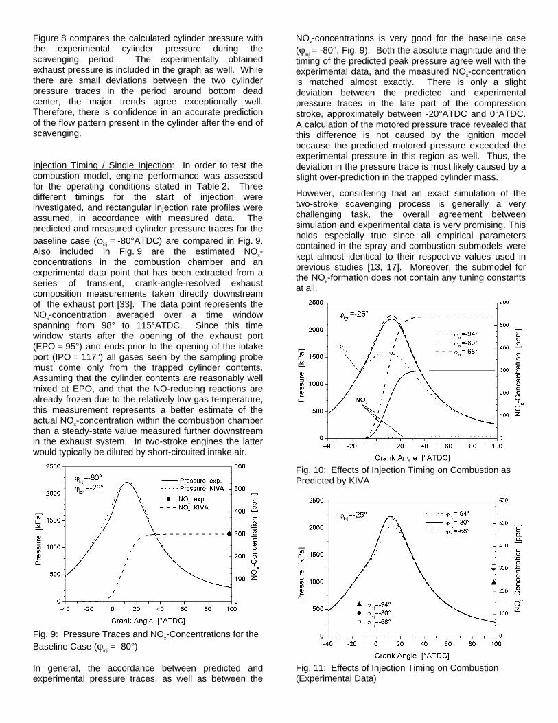
Figure 8 compares the calculated cylinder pressure with the experimental cylinder pressure during the scavenging period. The experimentally obtained exhaust pressure is included in the graph as well. While there are small deviations between the two cylinder pressure traces in the period around bottom dead center, the major trends agree exceptionally well. Therefore, there is confidence in an accurate prediction of the flow pattern present in the cylinder after the end of scavenging.

Injection Timing / Single Injection: In order to test the combustion model, engine performance was assessed for the operating conditions stated in Table 2. Three different timings for the start of injection were investigated, and rectangular injection rate profiles were assumed, in accordance with measured data. The predicted and measured cylinder pressure traces for the baseline case (ϕinj = -80°ATDC) are compared in Fig. 9. Also included in Fig. 9 are the estimated NOx-concentrations in the combustion chamber and an experimental data point that has been extracted from a series of transient, crank-angle-resolved exhaust composition measurements taken directly downstream of the exhaust port [33]. The data point represents the NOx-concentration averaged over a time window spanning from 98° to 115°ATDC. Since this time window starts after the opening of the exhaust port (EPO = 95°) and ends prior to the opening of the intake port (IPO = 117°) all gases seen by the sampling probe must come only from the trapped cylinder contents. Assuming that the cylinder contents are reasonably well mixed at EPO, and that the NO-reducing reactions are already frozen due to the relatively low gas temperature, this measurement represents a better estimate of the actual NOx-concentration within the combustion chamber than a steady-state value measured further downstream in the exhaust system. In two-stroke engines the latter would typically be diluted by short-circuited intake air.

Fig. 9: Pressure Traces and NOx-Concentrations for the Baseline Case (ϕinj = -80°)

In general, the accordance between predicted and experimental pressure traces, as well as between the

NOx-concentrations is very good for the baseline case (ϕinj = -80°, Fig. 9). Both the absolute magnitude and the timing of the predicted peak pressure agree well with the experimental data, and the measured NOx-concentration is matched almost exactly. There is only a slight deviation between the predicted and experimental pressure traces in the late part of the compression stroke, approximately between -20°ATDC and 0°ATDC. A calculation of the motored pressure trace revealed that this difference is not caused by the ignition model because the predicted motored pressure exceeded the experimental pressure in this region as well. Thus, the deviation in the pressure trace is most likely caused by a slight over-prediction in the trapped cylinder mass.

However, considering that an exact simulation of the two-stroke scavenging process is generally a very challenging task, the overall agreement between simulation and experimental data is very promising. This holds especially true since all empirical parameters contained in the spray and combustion submodels were kept almost identical to their respective values used in previous studies [13, 17]. Moreover, the submodel for the NOx-formation does not contain any tuning constants at all.

Fig. 10: Effects of Injection Timing on Combustion as Predicted by KIVA

Fig. 11: Effects of Injection Timing on Combustion (Experimental Data)

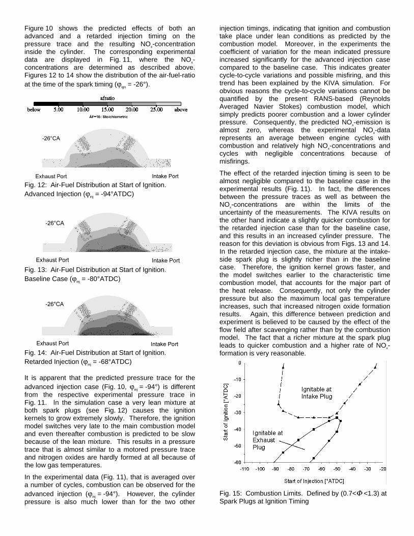
Figure 10 shows the predicted effects of both an advanced and a retarded injection timing on the pressure trace and the resulting NOx-concentration inside the cylinder. The corresponding experimental data are displayed in Fig. 11, where the NOx-concentrations are determined as described above. Figures 12 to 14 show the distribution of the air-fuel-ratio at the time of the spark timing (ϕign = -26°).

Fig. 12: Air-Fuel Distribution at Start of Ignition. Advanced Injection (ϕinj = -94°ATDC)

Fig. 13: Air-Fuel Distribution at Start of Ignition. Baseline Case (ϕinj = -80°ATDC)

Fig. 14: Air-Fuel Distribution at Start of Ignition. Retarded Injection (ϕinj = -68°ATDC)

It is apparent that the predicted pressure trace for the advanced injection case (Fig. 10, ϕinj = -94°) is different from the respective experimental pressure trace in Fig. 11. In the simulation case a very lean mixture at both spark plugs (see Fig. 12) causes the ignition kernels to grow extremely slowly. Therefore, the ignition model switches very late to the main combustion model and even thereafter combustion is predicted to be slow because of the lean mixture. This results in a pressure trace that is almost similar to a motored pressure trace and nitrogen oxides are hardly formed at all because of the low gas temperatures.

In the experimental data (Fig. 11), that is averaged over a number of cycles, combustion can be observed for the advanced injection (ϕinj = -94°). However, the cylinder pressure is also much lower than for the two other

injection timings, indicating that ignition and combustion take place under lean conditions as predicted by the combustion model. Moreover, in the experiments the coefficient of variation for the mean indicated pressure increased significantly for the advanced injection case compared to the baseline case. This indicates greater cycle-to-cycle variations and possible misfiring, and this trend has been explained by the KIVA simulation. For obvious reasons the cycle-to-cycle variations cannot be quantified by the present RANS-based (Reynolds Averaged Navier Stokes) combustion model, which simply predicts poorer combustion and a lower cylinder pressure. Consequently, the predicted NOx-emission is almost zero, whereas the experimental NOx-data represents an average between engine cycles with combustion and relatively high NOx-concentrations and cycles with negligible concentrations because of misfirings.

The effect of the retarded injection timing is seen to be almost negligible compared to the baseline case in the experimental results (Fig. 11). In fact, the differences between the pressure traces as well as between the NOx-concentrations are within the limits of the uncertainty of the measurements. The KIVA results on the other hand indicate a slightly quicker combustion for the retarded injection case than for the baseline case, and this results in an increased cylinder pressure. The reason for this deviation is obvious from Figs. 13 and 14. In the retarded injection case, the mixture at the intake-side spark plug is slightly richer than in the baseline case. Therefore, the ignition kernel grows faster, and the model switches earlier to the characteristic time combustion model, that accounts for the major part of the heat release. Consequently, not only the cylinder pressure but also the maximum local gas temperature increases, such that increased nitrogen oxide formation results. Again, this difference between prediction and experiment is believed to be caused by the effect of the flow field after scavenging rather than by the combustion model. The fact that a richer mixture at the spark plug leads to quicker combustion and a higher rate of NOx-formation is very reasonable.

Fig. 15: Combustion Limits. Defined by (0.7<Φ <1.3) at Spark Plugs at Ignition Timing

Figure 15 shows a predicted map of ignition timing versus injection timing that identifies regions which allow stable combustion for the engine load and speed specified in Tab. 2. The map was established by running the proposed models for various injection timings and assuming that stable combustion can be achieved for those ignition timings, at which the gas equivalence ratio at one of the spark gaps is within the ignitable limits of 0.7 and 1.3. Thus, for each injection timing a time span for possible ignition timings was determined for each of the two spark plugs, such that the two areas of ignitable injection-/ ignition-timing combinations shown in Fig. 15 were obtained. The upper area represents the spark plug located on the intake port side of the combustion chamber (right hand side in Figs. 12 to 14) and the lower area represents the plug located on the exhaust port side.

According to test engine data, an injection duration of 12°CA with a rectangular injection rate profile was chosen for all runs included in Fig. 15. The injected fuel mass was kept constant for all investigated injection timings.

The results show that for the engine operating conditions specified in Tab. 2, the exhaust side spark plug requires generally an earlier ignition timing than the intake side plug. This can be explained by the counter-clockwise tumble inside the cylinder, that is of mediocre strength for the chosen engine speed. The airflow deflects the injected fuel towards the exhaust plug while it is still in the upper half of the cylinder dome. Once the fuel reaches the region near the piston, it is shifted to the intake port side again, and finally up towards the intake side plug.

Two main conclusions can be drawn from Fig. 15. Firstly, the range of those injection-/ ignition-timing combinations yielding strong and stable combustion that can be selected in order to optimize the typical trade-off between fuel consumption and NOx-emissions can be enlarged significantly by using two spark plugs instead of only one. This is especially the case if one considers that the sizes, shapes and locations of the two areas displayed in Fig. 15 will change for different load and speed conditions of the engine. For example, for a higher engine speed the tumble in the combustion chamber will intensify such that the fuel vapor will be deflected more quickly and the combustible area corresponding to the exhaust side plug is likely to increase and move to a later ignition timing while the area representing the intake side plug will most probably shift to earlier timings. The second conclusion is drawn from the fact that the two areas representing the spark plugs do not intersect. This suggests that engine performance could most likely be enhanced by choosing an independent ignition timing for each of the plugs. The most stable and quickest combustion – that could however, cause drawbacks with respect to NOx-formation and engine knock – will typically result for ignition timings chosen well within the indicated limits of ignition/combustion for the respective plugs indicated in Fig. 15.

With the spray and combustion models described above, plots similar to Fig. 15 can be created for various load and speed conditions of an engine. Iso-curves for particular equivalence ratios that have been proven desirable for ignition of the specific engine can then easily be included, such that the proposed combustion model can be viewed as a powerful tool to simplify the search for a map of suitable injection- and ignition-timings of a DISC engine.

CONCEPTUAL STUDY ON SPLIT INJECTIONS: The proposed model was applied to study the effects of split injections on combustion characteristics and engine performance for the same operating conditions of the DISC two-stroke engine specified in the previous section. In order to keep the number of parameters for this study manageable, only injection cases with two pulses of equal duration (6°CA each) were considered. Consequently, each pulse contained exactly 50% of the total fuel mass injected in the single injection cases. Moreover, to enable a direct comparison of the split injection results to the single injection results, the second injection pulse was always timed such that its end was equal to the end of injection of the respective single injection case (see Fig. 16). The start of the first injection pulse was varied in increments of 6°CA up to a timing of -110°ATDC, which represents the earliest start of injection that still eliminates the possibility of fuel getting short-circuited directly into the exhaust port of the two-stroke engine (EPC=-95°ATDC).

Fig. 16: Timing for Split Injection Pulses

Two series of split injection calculations were performed, corresponding to the baseline and retarded single injection cases of the previous section. In the first series of runs (corresponding to the baseline case) the second injection pulse was fixed, starting at -74° and ending at -68°ATDC, while the timing of the first pulse was varied. In the second series of runs (corresponding to the retarded injection case) the second pulse was fixed at -62° to -56°ATDC and the timing of the first pulse was varied again.

The injection-/ ignition-timing combinations yielding stable combustion are displayed in Figs. 17 and 18 for these two series of calculations, respectively. Compared

to the single injection results (Fig. 15), it can be seen that for both series of split injections the possible start of ignition at the exhaust side plug can be extended to a later timing by up to 20°CA. On the other hand, the time windows for possible ignition at the intake side plug decrease for an earlier start of injection of the first pulse. However, in spite of this shortening at the intake plug, Fig. 18 suggests that a split injection can be designed which allows simultaneous ignition at both spark plugs (i.e., in contrast to Fig. 15 the areas representing the two spark plugs do intersect in Fig. 18). The corresponding time window during that ignition at both plugs is possible is located between approximately –30° and –15°CA, which is very favorable for combustion under the given operating conditions. Hence, the combination of two spark plugs and split injections can be utilized to design a strong ignition and stable combustion, when the later timing for the second injection pulse (-62° to –56°) is selected.

Fig. 17: Combustion Limits (0.7<Φ<1.3 at Spark Plugs) for Split Injection. 2nd Pulse Fixed at –74° to –68°ATDC

Fig. 18: Combustion Limits (0.7<Φ<1.3 at Spark Plugs) for Split Injection. 2nd Pulse Fixed at –62° to –56°ATDC

The reason for the described changes in the injection-/ ignition-timing maps can be concluded by examining the histories of the air-fuel ratio distributions in the combustion chamber for a typical split injection case and for a single injection case as shown in Figs. 19 and 20, respectively. As the top plot in Fig. 19 (ϕ=-60°ATDC) indicates, the fuel injected during the early first pulse is already diluted to an air-fuel ratio of about 20 when the second injection pulse starts. Since early in the compression stroke the counter-clockwise tumble is not yet strongly developed, this fuel cloud resulting from the first injection pulse tends to stay on the left side of the cylinder (i.e., on the exhaust port side). And even though the evaporation rate of the liquid fuel droplets – represented by the dots in Figs. 19 and 20 – is slow due to the low gas temperature at an early injection timing, there is no excessive amount of liquid fuel impinging on the piston surface. This is simply due to the fact that the early injected fuel can travel a longer distance from the injector until it reaches the piston.

At –40°ATDC the fuel clouds resulting from the two different pulses have mixed. However, the air-fuel distribution is much different than in the corresponding single injection case of Fig. 20. Due to the early first injection pulse, that almost reaches into the squish region near the exhaust port, the fuel cloud stays more to the left and extends further into the cylinder dome. An additional effect is that an early injection pulse just after EPC counteracts the development of a strong tumble. Therefore, the counter-clockwise trajectory of the injected fuel is diminished.

Because only 50% of the total fuel mass is injected at a late timing when the piston is close to the injector, the amount of liquid fuel impinging on the piston surface can be limited. Consequently, the amount of extremely rich mixture close to the piston is also reduced. Overall the fuel cloud caused by the split injection is narrower, shifted towards the exhaust side and extends further up into the cylinder dome than the one resulting from a single injection.

At –26°ATDC, which was chosen as the ignition timing for all combustion calculations in this study, similar trends can be observed. For the split injection, there is less liquid fuel and less rich mixture close to the piston surface and the regions of intermediate and lean mixture extend further towards the exhaust side spark plug. On the other hand, the weaker tumble caused by the early first injection pulse delays the movement of the fuel cloud up into the dome area and towards the intake side spark plug. This is the main reason why the intake plug areas in Figs. 17 and 18 are smaller and start at a later ignition timing than for the single injection cases displayed in Fig. 15. However, in the split injection case represented in Fig. 19 the air-fuel ratio at the spark gap is still comparable to the one in the single injection case, such that stable ignition and combustion are predicted. In fact, since the flamefront can be initiated at both plugs for the presented split injection case, the mixture starts to burn even more quickly.

Fig. 19: Development of Air-Fuel Distribution for Split Injection. Pulse 1: -92° to –86°. Pulse 2: -62° to –56°.

Fig. 20: Development of Air-Fuel Distribution for Single Injection. Inj. Timing: -68° to –56°.

The latter aspect is further explored in Fig. 21, which shows predicted peak combustion pressures resulting from various injection timings for both single and split injection cases. The ignition timing was kept constant for all investigated cases at -26°ATDC. Since the total mass of injected fuel is also identical in each of the cases, the peak pressure can provide an estimate of the specific fuel consumption. A higher peak pressure occurring at roughly the same timing typically means a better efficiency of the engine.

Fig. 21: Peak Cylinder Pressure for Various Injection Strategies

The graph shows that the split injection with the retarded second pulse (-62° to –56°ATDC) can yield a higher maximum cylinder pressure than the baseline and retarded single injection cases that are also included in Fig. 21. This is due to the fact that ignition can take place at two different locations in the cylinder such that the early stages of combustion proceed more quickly. For the split injection cases with the second pulse timed between -74° and –68° ATDC, the very low peak pressures indicate that there is hardly any combustion taking place for the chosen ignition timing of -26°. This agrees to the results in Fig. 17 that show that no stable combustion can be achieved for this particular ignition timing at either spark plug.

The cylinder averaged concentrations of nitrogen oxides and unburned fuel at EPO that correspond to the above peak pressures are displayed in Figs. 22 and 23. As it was expected the cases without sufficient combustion are characterized by extremely low NOx-concentrations and large amounts of unburned fuel. However, comparing the split injection cases that do yield satisfactory combustion (retarded second pulse) and the single injection cases, the graphs suggest that a split injection can be designed that allows a combustion with higher peak pressure (i.e., a lower specific fuel consumption), comparable emissions of unburned fuel and equal or even lower NOx-emissions. Specifically, this is the case for split injections with the start of the first pulse varying between –92 and –80°ATDC and the start of the second pulse fixed at –62°ATDC.

Taking into account the results of Fig. 19 this behavior can be explained as follows. The late second pulse of the injection supplies a stratified charge that is sufficiently rich to initiate combustion at the intake plug. At the same time, the fuel of the earlier first pulse penetrates into a region of the cylinder that is not that strongly affected by the tumble flow. Therefore, it tends to stay on the exhaust port side of the combustion chamber and enables ignition at the exhaust side plug. Due to the flame initiations at two different positions in the cylinder, the early part of combustion can proceed more quickly such that the spatially integrated rate of heat release is increased and an improved engine efficiency is obtained. However, since each injection pulse contains only 50 % of the total fuel mass, the fraction of fuel that burns rapidly in a stoichiometric or rich mixture and results in high local temperatures is limited. A greater amount of fuel has been more diluted with air and burns under leaner conditions (AF-ratio between 20 and 25). Thus, high local temperatures are avoided and the rate of nitrogen-oxide formation can be controlled.

Another reason for the lower NOx-concentration in the split injection case could be that there is less liquid fuel evaporating off the piston surface because of the smaller amount of fuel injected late when the piston is close to the injector. Consequently a greater fraction of energy that is required for the evaporation is subtracted from the cylinder gases rather than the piston. Therefore, the gas temperature stays lower, which is favorable for low NOx-formation.

Fig. 22: In-Cylinder NOx-Concentrations for Various Injection Strategies

Similar positive effects of split injections have been found by Kuwahara et al. [35] in an experimental study performed on a DISC four-stroke engine. Among other results they concluded that a richer mixture at the spark plug is beneficial for a quick initiation of the flame and a more diluted mixture resulting from an early pulse helps controlling engine knock that is typically caused if combustion takes place too fast.

The agreement between the two studies is very promising, as it indicates that general trends resulting

from various injection and ignition strategies can be predicted well with the current combustion model. Therefore, the model represents a powerful tool for further improvements in engine design.

Fig. 23: In-Cylinder Concentrations of Unburned Fuel for Various Injection Strategies

CONCLUSIONS

A liquid sheet atomization model for pressure-swirl injectors has been combined with a phenomenological ignition model that tracks the initial growth of the flame kernel with Lagrangian marker particles. The models have been advanced in this analysis to allow the simulation of multiple spark plugs as well as split injections and have been applied in order to study a small marine DISI two-stroke engine with a modified KIVA-3 code.

In a first step, the spray model has been validated independently of the ignition and combustion models by calculating a non-evaporating spray in a pressure bomb under various boundary conditions. A good agreement was found between predicted results and experimental data such that there is confidence in the predictive quality of the spray model.

The complete model has then been applied to study the DISI two-stroke engine operating in a late injection, stratified charge mode typical of part load conditions. Predicted engine performance has been compared to experimental data for three different injection timings. While the accordance for the baseline case is exceptionally good, deviations in the absolute quantities for cylinder pressures and NOx-emissions can be observed for the advanced and retarded injection timings. These deviations are most likely caused by an uncertainty in the flow field present after the scavenging process of the two-stroke engine, for which only limited experimental data was available. However, the general trends caused by a change in injection timing have been predicted correctly.

Finally, a conceptual study about the effect of split injections has been performed for the same DISI two-stroke engine. In this study the simulation model has

been proven to be a valuable tool in engine design, since it allows to establish maps of injection-/ ignition-timing combinations that ensure stable combustion without misfiring that is crucial in DISC engines, especially at part load conditions. Moreover, the model has been successfully used to identify optimum timings for split injections. A potential has been found to improve the engine’s specific fuel consumption compared to single injection operation while the unburned fuel emissions remain approximately unchanged and NOx-formation can even be slightly reduced.

Specifically, the simulation results suggest that a two-pulse injection with 50% of the fuel mass injected directly after the closing of the exhaust port and the remaining 50% injected approximately 30°CA later represents the optimum for the investigated part load conditions. The late injected fuel of the second pulse is still stratified at the ignition timing such that a sufficiently rich mixture at the spark plug ensures a stable initiation of combustion. In contrast, the fuel injected during the early first pulse is more diluted and results in a reduced maximum combustion temperature such that formation of nitrogen oxides can be controlled.

ACKNOWLEDGMENTS

This work was supported by Ford. The authors thank Dr. Li Fan (Ford), and Prof. Jaal Ghandhi and Prof. P. Farrell and W.S. Chang (ERC) for supplying experimental data.

NOMENCLATURE

Latin Symbols:

C constant cD drag coefficient d0 nozzle diameter dD droplet diameter E activation temperature h sheet half-thickness k wave number, turbulent kinetic energy kv discharge coefficient L sheet breakup length ll integral turbulent length scale m mass flow rate MW molecular weight Np number of particles p pressure Q density ratio ρg/ρl R residual mass fraction r radius sL laminar flame speed T Temperature t time tf film thickness inside the nozzle exit U total fuel velocity u axial velocity component uk,rad ignition kernel growth speed V volume We Weber number

Y mass fraction y drop distortion parameter Greek Symbols

ε dissipation rate of turb. kin. energy Φ equivalence ratio η surface disturbance ϕ crank angle µ dynamic viscosity λ wave length ν kinematic viscosity θ spray half-cone angle ρ density Σ flame surface density σ surface tension τb sheet breakup time τc chemical time scale τl laminar time scale τt turbulent time scale Ω growth rate of most unstable disturbance ω disturbance growth rate Subscripts and Superscripts:

ad adiabatic amb ambient b breakup F fuel g gas i species ign ignition inj injection k ignition kernel L ligament l liquid, laminar P product S start of ignition t turbulent 0 initial * equilibrium composition Abbreviations:

ATDC after top dead center CA crank angle DISC direct injection stratified charge DISI direct injection spark ignition DPIK discrete particle ignition kernel EPC exhaust port closure EPO exhaust port opening IPC intake port closure IPO intake port opening LISA linearized instability sheet atomization TAB Taylor-Analogy-Breakup

REFERENCES

[1] Anderson, R.W., Yang, J., Brehob, D.D., Vallance, J.K., Whiteaker, R.M.: Understanding the Thermodynamics of Direct Injection Spark Ignition (DISI) Combustion Systems: An Analytical and Experimental Investigation; SAE Paper 962018, 1996

[2] Fraidl, G.K., Piock, W.F., Wirth, M.: Gasoline Direct Injection: Actual Trends and Future Strategies for Injection and Combustion Systems; SAE Paper 960465, 1996

[3] Zhao, F.Q., Lai, M.C., Harrington, D.L.: A Review of Mixture Preparation and Combustion Control Strategies for Spark-Ignited Direct-Injection Gasoline Engines; SAE Paper 970627, 1997

[4] Amsden, A.A., O’Rourke, P.J., Butler, T.D.: KIVA-II – A Computer Program for Chemically Reactive Flows with Sprays; Los Alamos National Laboratory LA-11560-MS, 1989

[5] Amsden, A.A.: KIVA-3: A KIVA Program with Block-Structured Mesh for Complex Geometries; Los Alamos National Laboratory LA-12503-MS, 1993

[6] Reitz, R.D.: Modeling Atomization Processes in High-Pressure Vaporizing Sprays; Atomization and Spray Technology, vol. 3, pp. 309-337, 1987

[7] O’Rourke, P.J., Amsden, A.A.: The TAB Method for Numerical Calculation of Spray Droplet Breakup; SAE Paper 872089, 1987

[8] Hwang, S.S., Liu, Z., Reitz, R.D.: Breakup Mechanisms and Drag Coefficients of High Speed Vaporizing Liquid Drops; Atomization and Sprays, vol. 6, no. 3, pp. 353-376, 1996

[9] Reitz, R.D., Diwakar, R.: Effect of Drop Breakup on Fuel Sprays; SAE Paper 860469, 1986

[10] Han, Z., Reitz, R.D., Claybaker, P.J., Rutland, C.J., Yang, J., Anderson, R.W.: Modeling the Effects of Intake Flow Structures on Fuel/Air Mixing in a Direct-Injected Spark-Ignition Engine; SAE Paper 961192, 1996

[11] Yi, J., Han, Z., Yang, J., Anderson, R., Trigui, N., Boussarsar, R.: Modeling of the Interaction of Intake Flow and Fuel Spray in DISI Engines; SAE Paper 2000-01-0656, 2000

[12] Han, Z., Parrish, S., Farrell, P.V., Reitz, R.D.: Modeling Atomization Processes of Pressure-Swirl Hollow-Cone Fuel Sprays; Atomization and Sprays, vol. 7, pp. 663-684, 1997

[13] Schmidt, D.P., Nouar, I., Senecal, P.K., Rutland, C.J., Martin, J.K., Reitz, R.D.: Pressure-Swirl Atomization in the Near Field; SAE Paper 1999-01-0496, 1999

[14] Arcoumanis, C., Gavaises, M.: Pressure-Swirl Atomizers for DISI Engines: Further Modeling and Experiments; SAE Paper 2000-01-1044

[15] O’Rourke, P.J., Amsden, A.A.: Three Dimensional Numerical Simulations of the UPS-292 Stratified Charge Engine; SAE Paper 870597, 1987

[16] Gill, A., Gutheil, E., Warnatz, J.: Numerical Investigation of the Combustion Process in a Direct-Injection Stratified Charge Engine; Combustion Science and Technology, vol. 115, pp. 317-333, 1996

[17] Fan, L., Li, F., Han, Z., Reitz, R.D.: Modeling Fuel Preparation and Stratified Combustion in a Gasoline Direct Injection Engine; SAE Paper 1999-01-0175, 1999

[18] Abraham, J., Bracco, F.V., Reitz, R.D.: Comparisons of Computed and Measured Premixed Charge Engine Combustion; Combustion and Flame, vol. 60, pp. 309-322, 1985

[19] Magnussen, B.F., Hjertager, B.H.: On Mathematical Modeling of Turbulent Combustion with Special Emphasis on Soot Formation and Combustion; 16th Symp. (Int.) Comb., The Combustion Institute, pp. 719-729, 1977

[20] Han, Z., Reitz, R.D.: Turbulence Modeling of Internal Combustion Engines Using RNG k-e Models; Comb Science and Technology, vol. 106, pp. 267-295, 1995

[21] Han, Z., Reitz, R.D.: A Temperature Wall Function Formulation for Variable-Density Turbulent Flows with Application to Engine Convective Heat Transfer Modeling; Int. J. Heat Mass Transfer, vol. 40, pp. 613-625, 1997

[22] Naber, J.D., Reitz, R.D.: Modeling Engine Spray/Wall-Impingement; SAE Paper 880107, 1988

[23] Senecal, P.K., Schmidt, D.P., Nouar, I., Rutland, C.J., Reitz, R.D., Corradini, M.L.: Modeling High-Speed Viscous Liquid Sheet Atomization; Int. J. Multiphase Flow, vol. 25, No. 6-7, pp. 1073-1097, 1999

[24] Squire, H.B.: Investigation of the Instability of a Moving Liquid Film; Brit. J. Appl. Phys., vol. 4, p. 167, 1953

[25] Heagerty, W.W., Shea, J.F.: A Study of the Stability of Plane Fluid Sheets; J. Appl. Mech., vol. 22, p. 509, 1955

[26] Reitz, R.D., Bracco, F.V.: Mechanism of Atomization of a Liquid Jet; The Physics of Fluids, vol. 25, p. 1730, Oct. 1982

[27] Dombrowski, N., Hooper, P.C.: The Effect of Ambient Density on Drop Formation in Sprays; Chem. Eng. Sci., vol. 17, p. 291, 1962

[28] Metghalchi, M., Keck, J.: Burning Velocities of Mixtures of Air with Methanol, Isooctane, and Indolene at High Pressure and Temperature; Combustion and Flame, vol. 48, pp.191-210, 1982

[29] Kuo, T.W., Reitz, R.D.: Three-Dimensional Computations of Combustion in Premixed-Charge and Direct-Injected Two-Stroke Engines; SAE paper 920425, 1992

[30] Heywood, J.B.: Internal Combustion Engine Fundamentals; McGraw Hill, 1988

[31] Chang, W.S., Farrell, P.V.: Comparison of Spray Characteristics for Two GDI Fuel Injectors; ASME Internal Combustion Engine Division Conference, 2000

[32] Fan, L., Reitz, R.D.: Multi-Dimensional Modeling of Mixing and Combustion of a Two-Stroke Direct-Injection Spark Ignition Engine; SAE Paper 2001-01-1228, 2001

[33] Hudak, E.: Time-Resolved Exhaust Measurements of a Two-Stroke Direct-Injection Engine; M.S. Thesis, University of Wisconsin-Madison, 1998

[34] Zhu, Y., Reitz, R.D.: A 1-D Gas Dynamics Code for Subsonic and Supersonic Flows Applied to Predict EGR Levels in a Heavy-Duty Diesel Engine; Int. J. Vehicle Design, vol. 22, pp. 227-252, 1999

[35] Kuwahara, K., Ueda, K., Ando, H.: Mixing Control Strategy for Engine Performance Improvement in a Gasoline Direct Injection Engine; SAE paper 980158, 1998