Fisheries and OceansScience

Pêches et OcéansSciences

C S A SCanadian Science Advisory Secretariat

S C C SSecrétariat canadien de consultation scientifique

* This series documents the scientific basis forthe evaluation of fisheries resources inCanada. As such, it addresses the issues ofthe day in the time frames required and thedocuments it contains are not intended asdefinitive statements on the subjectsaddressed but rather as progress reports onongoing investigations.

* La présente série documente les basesscientifiques des évaluations des ressourceshalieutiques du Canada. Elle traite desproblèmes courants selon les échéanciersdictés. Les documents qu’elle contient nedoivent pas être considérés comme desénoncés définitifs sur les sujets traités, maisplutôt comme des rapports d’étape sur lesétudes en cours.

Research documents are produced in theofficial language in which they are provided tothe Secretariat.

This document is available on the Internet at:

Les documents de recherche sont publiés dansla langue officielle utilisée dans le manuscritenvoyé au Secrétariat.

Ce document est disponible sur l’Internet à:http://www.dfo-mpo.gc.ca/csas/

ISSN 1480-4883Ottawa, 2001

Research Document 2001/083 Document de recherche 2001/083

Not to be cited withoutpermission of the authors *

Ne pas citer sansautorisation des auteurs *

2001 Stock Status Assessment of Coho Salmon from the InteriorFraser River

J. R. Irvine1, C. K. Parken1, D. G. Chen2, J. Candy1, T. Ming1, J. Supernault1, W. Shaw3, and R. E. Bailey4

1Fisheries and Oceans Canada Science Branch, Pacific Biological Station

3190 Hammond Bay RoadNanaimo, B.C. V9R 5K6

2International Pacific Halibut CommissionP.O. Box 95009

Seattle, Washington 98145-2009

3Fisheries and Oceans CanadaOperations Branch, South Coast Division

3225 Stephenson Point RoadNanaimo, B.C. V9T 1K3

4 Fisheries and Oceans CanadaScience Branch, Stock Assessment Division

1278 Dalhousie DriveKamloops, B.C. V2B 6G3

2

Abstract

The extreme fishery management measures undertaken in BC since 1998 to conserve coho appear to havestopped the declining trend for interior Fraser coho populations. We evaluated the impacts of continuedrestrictions in salmon harvest on the status of coho salmon of the interior Fraser River, including theThompson drainage in 2000. Fishery exploitations in 2000 were the lowest on record, ~3.4% in total, ofwhich half was in British Columbia. Fishery exploitations the last two years were low enough thatspawner numbers generally exceeded brood escapements. Productivity measured in recruits per spawnerhas improved and populations are now above replacement levels.

A mark-recapture program that used fishwheels in the Fraser Canyon as marking platforms provided anindependent estimate of spawner numbers in the interior Fraser watershed, as well as useful informationon stock composition. Results indicated that spawner surveys may be missing significant numbers ofcoho, particularly in non-Thompson streams. Additional survey work is required to verify the distributionof coho in the upper Fraser watershed, determine abundance, and collect baseline genetic samples.

We updated our information on the population structure of interior Fraser coho, and present evidence thatindicates that major drainage basins (e.g. North and South Thompson) may need to be considered asseparate Conservation Units. We discuss reference points for various coho populations and presentseveral values calculated using data from North Thompson coho. The mean of two minimum referencepoints was 5.2 female spawners per kilometer of accessible habitat. We presume that a limit referencepoint for North Thompson coho would be greater than or equal to this value. Since coho escapements inthe North Thompson watershed have been near but generally below this provisional reference point thepast four years, we conclude that the viability of these fish remains at risk. This finding, combined withthe short-term forecast for Thompson coho of continued poor survivals, leads to our recommendation thata cautious approach to fisheries management needs to remain in place in order to allow these populationsthe opportunity to rebuild.

The major recommendations from this research document are:1. More extensive baseline coverage of interior Fraser coho, especially in non-Thompson tributaries

upstream of the Fraser-Thompson confluence are required to aid in the delineation of populations andConservation Units, and provide more precise estimates of the distribution and numbers of interiorFraser coho in catches.

2. Rates of genetic exchange between generations and among populations need to be determined.3. To enable more effective fisheries management, coho encounter and DNA based stock composition

information should be used to develop a model of coho marine distribution and migratory timing.4. Although benefits can be seen from the extreme fishery management measures taken in recent years,

these measures should remain in place to permit populations the opportunity to rebuild.

3

Résumé

Les mesures radicales de gestion des pêches prises en Colombie-Britannique depuis 1998 en vue deprotéger le saumon coho semblent avoir stoppé la tendance à la baisse des populations du cours supérieurdu Fraser. Sont évaluées dans le présent document les répercussions des limites des prises de saumon surl'état du stock de coho du cours supérieur du Fraser, y compris le bassin versant de la rivière Thompson,en 2000. Les prises en 2000 étaient les plus faibles enregistrées, soit environ 3,4 % du total des effectifs,dont la moitié ont été récoltées en Colombie-Britannique. Les prises au cours des deux dernières annéesétaient tellement faibles que le nombre de géniteurs était généralement supérieur à l'échappée. Laproductivité, mesurée en nombre de recrues par géniteur, a augmenté et les populations se situentmaintenant au-dessus des niveaux de remplacement.

Un programme de marquage et de recapture utilisant des filets rotatifs installés dans le canyon du Frasercomme plates-formes de marquage a donné une estimation indépendante du nombre de géniteurs dans lecours supérieur du Fraser, ainsi que des renseignements utiles sur la composition du stock. Les résultatsrévèlent que les relevés de géniteurs ignorent peut-être un grand nombre de coho, en particulier dans lescours d'eau autres que la Thompson. D'autres travaux sont requis pour vérifier la distribution du cohodans le cours supérieur du Fraser, établir son abondance et prélever des échantillons de matériel génétiquede base.

Les renseignements sur la structure de la population du coho du cours supérieur du Fraser ont été mis àjour et des éléments probants sont présentés qui indiquent que les principaux bassins versants (p. ex., laThompson Nord et la Thompson Sud) devraient peut-être être considérés comme des unités deconservation distinctes. Les points de référence de diverses populations de coho sont examinés etplusieurs valeurs, calculées à partir de données sur le coho de la Thompson Nord, présentées. La moyennede deux points de référence minimums se chiffre à 5,2 géniteurs femelles par km d'habitat facile d'accès.On suppose qu'un point de référence limite pour le coho de la Thompson Nord serait égal ou supérieur àcette valeur. Étant donné que les échappées de coho dans le bassin versant de la Thompson Nord serapprochaient de ce point de référence moyen, mais sans y être égal, au cours des quatre dernières années,on conclut que la viabilité de ces géniteurs reste menacée. Cette conclusion, jointe au fait que l'on prévoità court terme que le coho de la Thompson continuera à souffrir d'un faible taux de survie, a mené à larecommandation à l'effet qu'il faut continuer de faire preuve de prudence dans la gestion des pêches afinde permettre à ces populations de se rétablir.

Suivent les principales recommandations formulées :1. Une couverture de base plus exhaustive du coho du cours supérieur du Fraser, en particulier des

tributaires autres que la Thompson en amont de la confluence de ces deux cours d'eau, est nécessairepour délimiter les populations et les unités de conservation et obtenir des estimations plus précises dela distribution et du nombre de coho du cours supérieur du Fraser dans les prises.

2. Les taux d'échange génétique inter-populations et intra-populations doivent être déterminés.3. Pour que la gestion des pêches soit plus efficace, l'information sur la présence du coho et la

composition des stocks établies par analyse de l'ADN devrait être utilisée pour élaborer un modèle dela distribution et de la chronologie de la migration du coho en mer.

4. Les mesures radicales de gestion des pêches mises en œuvre dans les dernières années, très efficaces,devraient continuer à s'appliquer afin de permettre aux populations de se rétablir.

4

Table of Contents

Abstract .......................................................................................................................................... 21.0 Introduction ............................................................................................................................. 82.0 Data Sources and Treatments ................................................................................................ 8

2.1 Genetic Information ..................................................................................................82.2 Spawner Escapement Surveys ....................................................................................92.3 Fraser Canyon Fishwheel Program............................................................................102.4 Fisheries.................................................................................................................102.5 Stock-Recruitment ..................................................................................................113.0 Population Structure of Interior Fraser Coho ..............................................................123.1 Stock Composition of Interior Fraser Coho ................................................................13

4.0 Spawner Escapements........................................................................................................... 144.1 Results from Spawner Surveys .................................................................................144.2 Population Size Estimates from Fishwheel Program....................................................154.3 Comparison Between Spawner Survey and Fishwheel Population Estimates .................154.4 Run Timing Through Fraser Canyon .........................................................................16

5.0 Catch and Exploitation ......................................................................................................... 166.0 Productivity............................................................................................................................ 177.0 Reference Points .................................................................................................................... 18

7.1 North Thompson reference points .............................................................................198.0 Summary and Conclusions................................................................................................... 209.0 Acknowledgements................................................................................................................ 2210.0 References Cited.................................................................................................................. 22

5

List of Tables

Table 1. Definitions of the fishwheel tag application site, fishwheel tag recovery site andmajor watershed codes corresponding to Figure 1. ................................................................. 25Table 2. Estimated percentage stock composition, with standard deviations in parentheses,for coho sampled at the Yale and Siska fishwheels. ................................................................. 26Table 3. Mean bias between trend and true escapement (esc.) estimates for major basinswithing the Interior Fraser Management Unit......................................................................... 27Table 4. Summary of statistical test results for sampling selectivity bias investigations inthe application (fishwheels) and recovery (tag recovery sites) samples. Data were stratifiedby tagging at Yale and Siska. ..................................................................................................... 27Table 5. Summary of mark-recapture parameters and pooled Petersen escapementestimates stratified by tagging at Yale and Siska. .................................................................... 28Table 6. Migration timing reference points from cumulative frequency distributions of thenormal curve, Poisson curve, and observed CPUE at the Gordon Creek fishwheel, 2000. . 28Table 7. Summary estimates of 2000 escapements, fishery mortalities, and exploitations forThompson watershed coho in fisheries in Alaska, North/Central BC, southern BC andWashington. ................................................................................................................................. 29Table 8. Generational rates of change for escapements of unenhanced coho salmonreturning to indicator stream aggregates in the South and North Thompson drainages. ... 29Table 9. Summary of provisional reference points for North Thompson coho salmon. Seetext for explanation (S = spawners). .......................................................................................... 29Table 10. Sex ratios for coho returning to streams in the North Thompson watershed1. ... 30

6

List of Figures

Figure 1. Known and suspected coho salmon distribution in the interior Fraser Riverwatershed. Numbers for the fishwheel tag application sites, fishwheel tag recovery sitesand major watersheds are defined in Table 1. ......................................................................... 31Figure 2. Neighbor joining dendrogram of Fraser River coho salmon populations based onFst values calculated from six microsatellite loci and two MHC class I and class II loci. Fstscale is shown on bottom left. ..................................................................................................... 32Figure 3. Proposed population structure for interior Fraser River coho salmon. *indicatesa high degree of uncertainty. Streams sampled for DNA analysis are listed but not enclosedin boxes. ........................................................................................................................................ 33Figure 6. Relationship between aggregate escapements to South and North Thompsonindicator streams. ........................................................................................................................ 35Figure 7. Adjusted historical escapement for coho salmon returning to the North, South,and lower Thompson watersheds (data are in Appendix 3).................................................... 36Figure 8. Relationship between escapements to 16 indicator streams in the SouthThompson plus escapements to the Eagle and Salmon rivers and adjusted historicalescapements to the South Thompson watershed. ..................................................................... 37Figure 9. Relationship between escapements to 10 indicator streams in the NorthThompson and adjusted historical escapements to the North Thompson watershed. ......... 37Figure 10. Migration timing of coho at Yale (the Wall and Gordon Creek) and Siska basedon CPUE (fish/hr) at the fishwheels from 1998 to 2000. Brackets indicate the seasonalperiods of fishwheel operation and the solid line indicates the three-day moving average.. 38Figure 11. Normal and Poisson migration timing curves fit by least squares to coho CPUEobserved at the Gordon Creek fishwheel, Yale, 2000. ............................................................. 39Figure 12. Time series of ran, the annual rate of population growth for Thompson cohosalmon. Each point is the average (+-SE) of four time series (North and South indicatorstream aggregates, Eagle and Salmon rivers). When r<0, populations are unable to replacethemselves, even in the absence of fishing................................................................................. 40Figure 13. Time series of ran, the annual rate of population growth of Thompson cohosalmon. Each point is the average (+-SE) of two time series (North and South indicatorstream aggregates). When r<0, populations are unable to replace themselves, even in theabsence of fishing......................................................................................................................... 40Figure 14. Exploitation rate estimates for Thompson watershed (North and Southindicator stream aggregates, Eagle and Salmon rivers) coho (solid line) and exploitationrates that would have maintained coho production at the brood year escapement level (i.e.St = St-3 ) (dashed line). ................................................................................................................ 41Figure 15. Exploitation rate estimates for Thompson watershed (North and Southindicator stream aggregates) coho (solid line) and exploitation rates that would havemaintained coho production at the brood year escapement level (i.e. St = St-3 ) (dashed line)........................................................................................................................................................ 41Figure 16. Annual estimates of numbers of female coho per kilometre within the NorthThompson watershed. Horizontal line indicates the mean of two possible limit referencepoints (5.2 females/km). .............................................................................................................. 42

7

List of Appendices

Appendix 1. Coho DNA mixed stock estimates for 1997-1999 sampling, N= number of fishin sample. Standard deviations are in brackets. Samples with * indicates 1998 and 1999samples analyzed in year 2000. Thompson and Upper Fraser combined for 1997 and 1998samples analyzed in 1998............................................................................................................ 43Appendix 2. Coho DNA mixed stock estimates for year 2000 sampling, N = number of fishin sample. Standard deviations are in brackets........................................................................ 49Appendix 3. Estimated fishery exploitation rates (expl), adjusted historical escapements(esc), marine fishery catches and total abundances (abund) for interior Fraser Riverwatershed coho salmon. .............................................................................................................. 51Appendix 4 Chen, D. G., J. R. Irvine, and A. Cass. Incorporating Allee effects in salmonstock-recruitment models and applications for determining reference points. Draftmanuscript (in review). ............................................................................................................... 52

8

1.0 IntroductionThis is the fourth annual assessment of coho salmon from the interior Fraser River watershed. The studyarea encompasses the Fraser River watershed upstream of Hells Gate and includes the Thompson River,the largest watershed within the Fraser River system. We follow the recommendation from last year’sassessment (Irvine et al. 2000b) that stated the upstream boundary of the management unit for interiorFraser coho should indicate the known distribution of coho. Coho are prevalent throughout theThompson watershed but their distribution in non-Thompson Fraser systems is not well known. They arerecorded as far upstream as the Nechako drainage (Fig. 1).

The primary objective of this report is to update our knowledge of the status of interior Fraser cohosalmon. As in previous assessments, we do this by revising and evaluating our time series of spawnerescapement and productivity (recruits per spawner) estimates. In addition, in response to arecommendation in last year’s assessment, we assess status for North Thompson coho by comparingabundance with provisional reference points developed for coho from this watershed. We also evaluatethe utility of a fishwheel program in the Fraser Canyon, and incorporate and discuss new information onthe population genetic structure of interior Fraser coho.

2.0 Data Sources and Treatments

2.1 Genetic InformationIn last year’s assessment (Irvine et al. 2000b), we provided a detailed discussion on the geneticsubstructuring of interior Fraser coho. In the current report, we assemble the time series of stockcomposition information used to assess fishery impacts, and we incorporate new baseline information in adiscussion of population structure.

As in other recent years, tissue samples were taken from coho caught in most fisheries. For mixed stocksamples analyzed during 2000, five microsatellite (Oki1, Oki10, Oki100, Oki101 and Ots101) and twoMHC (alpha 1 and alpha 2) loci were used.

The coho salmon coast-wide baseline currently consists of approximately 22,000 fish from 141 stocksranging from southeastern Alaska to the Columbia River. An additional three stocks have been added tothe baseline since our previous assessment. These additional populations are the Nahatlatch River, FraserCanyon (~ 220 fish), Chapman Creek, Southern Mainland (~130 fish), and Chase River, East coast ofVancouver Island (~130 fish).

As in earlier assessments, we used three baseline sets of populations (including the three additionalstocks) for estimation of stock compositions in marine fisheries in British Columbia (see Appendix 1 inIrvine et al. 2000b). These three baselines were developed to account for the likely origin of coho salmonin specific fisheries. To minimize bias, we did not include populations in the baseline if they were highlyunlikely to be encountered in a fishery. Stock compositions for fishery samples from Statistical Areas 14-23 and 28-29 and Washington State were estimated with a “southern baseline”. The southern baselineincluded 85 populations, with populations from Oregon, Washington, the Fraser River, Vancouver Island,and the southern BC mainland for analysis. Stock compositions for samples from Areas 6-13 and 24-27were estimated with the “central baseline” that included all populations except Alaska. Stockcompositions for samples from northern Areas 1-6 were estimated with the “northern baseline” thatincluded all 142 populations in the analysis. Drainage-specific baseline populations were used to estimatestock compositions in freshwater fisheries in the Fraser River.

9

Maximum likelihood estimates (MLE) of stock grouping contributions were produced using the StatisticsProgram for Analyzing Mixtures (Debevec et al. 2000). Mixtures and baselines were bootstrapped 100times to generate standard deviations about each point estimate.

Stock composition estimates for fisheries sampled during 1997-1999 are provided in Appendix 1, andresults of analysis of 2000 samples are in Appendix 2. Although preliminary results from 1997-1999were provided in earlier assessments, Appendix 1 contains results from the analysis of additional samplesfrom this period and therefore replaces those results in earlier reports.

2.2 Spawner Escapement SurveysAnalysis of spawner escapement data provides the basis for many of our inferences about the status ofinterior Fraser coho. Some escapement estimates are obtained using a counting fence (with or withoutmark-recapture), others while drifting a stream in a vessel or by snorkeling, on foot, and from ahelicopter. Previous assessments (Irvine et al. 1999a, b, 2000b) describe these field studies in detail.

We were concerned with the accuracy and precision of our escapement time series. We expected thatmany estimates were biased low for a variety of reasons including difficulties in seeing all fish andsurveyors only sampling portions of many streams. We modified our sampling procedures commencing1998 to evaluate bias (i.e. accuracy). Before the 1998 field season began, we assembled detailed streamescapement histories going back to 1990 for as many systems as we could (Irvine et al. 1999b, Appendix3). For each stream/year combination, we documented the field technique and location where fish werecounted, and the analytical or other methods used to generate the escapement estimate from the field data.For most systems since 1998, two separate escapement estimates were generated. The first was our bestestimate of the true number of coho in the system that resulted from our increased survey effort. Thesecond was what we refer to as a trend estimate which is the probable number of fish that would havebeen estimated if survey effort had been similar to other recent years. We refer to these as estimates ofthe true escapement and the trend escapement.

As in last year’s assessment, two approaches were used to examine trends in spawner numbers. The first,an escapement indicator approach, relied on escapement estimates to unenhanced North and SouthThompson streams with reasonably consistent monitoring. Results provided in this report are the totalnumbers estimated to return to spawn in 10 unenhanced streams in the North Thompson, and 16unenhanced streams in the South Thompson and have not been corrected for bias. Details on theapproach are provided in earlier assessments (Irvine et al. 1999a, 1999b, 2000b).

The second time series approach used an escapement time series that included estimates for all streams.Using procedures documented in the most recent forecast document for southern B.C. coho (Simpson etal. 2001), total numbers of coho salmon spawners returning to the major basins within the Thompsonwatershed were estimated (Appendix 3). The complete escapement data set post-1975 was used, ratherthan only indicator stream data as described in the previous paragraph. Escapement estimates since 1975were adjusted upwards based on individual stream estimates of the ratio between the estimate of the trueescapement and the trend estimate. Missing escapement values were estimated. The escapement timeseries since 1998 consisted of our best estimates of the true numbers of coho spawning in each system.Streams draining into the North and South Thompson rivers have the longest and most complete timeseries of consistently generated estimates, streams of the lower Thompson/Nicola watersheds have ashorter time series, and non-Thompson interior Fraser streams have a short and relatively poor history ofcoho spawner records (Appendix 3).

10

2.3 Fraser Canyon Fishwheel ProgramThe primary stock assessment objectives of the fishwheel program were to generate spawner escapementestimates that were independent of those from escapement surveys, to document run timing, and toinvestigate temporal patterns of stock composition. In 2000, the program was expanded from the singlefishwheel operated in 1998 and 1999 at Yale, to two fishwheels near Yale and one near Siska (Fig. 1).Yale is at the downstream end of the Fraser Canyon, whereas Siska is upstream of the Fraser Canyon,about 15 km downstream of the Fraser and Thompson river confluence. Coho escapements wereestimated by mark-recapture by applying tags at the fishwheels and later inspecting coho at the fishwheeltag recovery sites.

The fishwheels were similar in design to those used for stock assessment on the Nass River (Link et al.1996). Each fishwheel, about 12.2 m long and 6.1 m wide, had three baskets on a rotating axle that couldcapture salmon as deep as about 4.2 m below the river surface. In 2000, fishwheels were operated duringmost of the coho migration period although time-periods varied among sites. Fishwheels operated 24h/day and results are provided as numbers caught per hour of fishwheel operation (CPUE). Near Yale,the Gordon Creek fishwheel operated longer (September 7 to October 24) than the Wall fishwheel(October 14 to 28), and also longer than the Siska fishwheel (September 22 to November 3). Coho weremarked with a uniquely numbered white (Yale) or yellow (Siska) jaw tag, applied to the lower jaw(Conrad et al. 2000). A circular (Yale) or square (Siska) hole punched in the operculum functioned as asecondary mark and as a source of tissue for genetic analyses. The sex, fork length, release condition, andfishwheel location and other data were recorded for all tagged coho.

Data from the two fishwheel locations were used to estimate somewhat different populations. Forexample, Nahatlatch River coho migrated by Yale, but they were unlikely to migrate past Siska, about 20km upstream of the Nahatlatch/Fraser River confluence. The recovery sample for Yale was constructedfrom live fish examined at counting fences, fishways, the Siska fishwheel and tangle netting (NahatlatchRiver), whereas the recovery sample for Siska was limited to live fish at counting fences and fishways.

Coho escapements past Yale and Siska were estimated with Chapman’s modification of the unbiasedPetersen estimator. Spatial, temporal, sex, size and fish stress biases were examined in the applicationand recovery samples following the methods described by Schubert (2000). Tagged coho probablyexperienced mortality rates in the range of 0 to 15% due to the capture, handling and tagging proceduresat the fishwheels. At the Nass River fishwheels, coho mortality was about 8% after capture, handling andradio tagging (Link and Gurak 1997), and we are unaware of other studies examining coho mortalityunder similar conditions. We assumed a 10% mortality rate for coho captured and tagged at thefishwheels based on the Nass River study and the condition of tagged coho observed at the fishwheel tagrecovery sites.

2.4 FisheriesIn 2000, salmon fisheries in southern BC continued to be managed to minimize mortalities of coho fromthe Thompson River watershed. Earlier assessments (Irvine et al. 1999a, 1999b, 2000b) describeapproaches used to assess fishery impacts on interior Fraser coho in detail and only a brief description ofthe approach is provided here. The approach used the last several years has been to allocate what wasconsidered to be an acceptable exploitation for Thompson coho in southern BC fisheries (~2%) amongstvarious fisheries. Fortunately, Thompson coho are sufficiently distinct genetically that we are reasonablyconfident in our ability to estimate numbers of Thompson-origin fish from mixed stock fishery samples.As most BC fisheries since 1997 have been non-retention for coho, few coho have been sampled forcoded-wire tags (CWTs). CWT recovery data alone would underestimate mortality in these fisheries inany case because they do not incorporate catch and release mortality. We applied stock composition

11

estimates developed using a DNA-based approach to estimates of coho killed in these fisheries(Appendices 1 and 2).

An in-season monitoring programme has been used the last several years to estimate coho encounters insouthern BC. Attempts were made to ensure that representative samples were taken from coho caught inmost fisheries. Samples were analyzed and estimated stock compositions (Appendix 2) were applied toencounter estimates from the 2000-monitoring programme to partition these amongst major populationaggregates. If we did not have an adequate sample size from the same or a nearby 2000 fishery during thesame or similar time period, we used stock composition estimates from sampling in earlier years(Appendix 1).

Coho mortalities in BC fisheries were determined by applying standard gear mortality estimates (sport10%, gill net 60%, troll 26%, and seine 25%) to the encounter data. Similar values, provided by Americancolleagues, were used to estimate the numbers of coho mortalities in mark-selective fisheries in Areas 5and 6 in WA. A description of the rationale for standard gear mortality estimates was provided in Irvineet al. (1999a). Additional work has taken place since these estimates were derived and new informationon gear and Canadian fishery specific mortality has recently become available. However, we did notupdate our gear mortality rates since there was insufficient time to review this new work.

Preliminary estimates of coho encounters and mortalities for fisheries in Washington State were providedto us by American colleagues. In 2000, selective mark-only sport fisheries operated in Washington Areas5 (Sekiu and Pillar Point) and 6 (East Juan de Fuca) but not in Area 7 San Juan Islands where cohoencounters were modest (J. Haymes, Wash. Dept. Fish. Wild. pers. comm.). DNA based estimates of theproportion made up by Thompson-origin fish were applied to estimates of the numbers of unmarked cohokilled in these fisheries. In addition, Boldt Treaty and non-treaty fisheries captured coho, and some ofthese coho would be of BC origin. Some commercial catch data were provided to us combined for Areas3+4, however, we assumed that there were no Thompson coho amongst catches from these areas. In2000, purse seines and reef nets were required to release coho from most areas (S. Boessow, Wash. Dept.Fish. Wild., pers. comm.), including those judged by us where they might capture migrating Thompsoncoho. Although gill-netters were allowed to keep coho, their coho catches were very small. Again, weused DNA evidence to estimate numbers of Thompson-origin mortalities amongst catches from Areas 4-7.

We did not have reliable estimates of mortalities or fishery exploitations for Thompson coho in Alaska orNorth/Central BC. We therefore assumed exploitation rates were the same as computed for 1999.

2.5 Stock-RecruitmentThe time series of exploitation rates for Thompson coho from MRP recoveries are summarized inAppendix 3 (see Appendix 3 in Irvine et al. 2000b for details). Estimates prior to 1986 were thearithmetic average of measured values from 1986 to 1996 (68%). Estimated exploitation in 1998 and1999 was approximately 7% and 9%, as previously reported (Irvine et al. 2000b). The estimatedexploitation rate in 2000 is 3.4% (Section 5.0).

Recruitment (catch plus spawning escapement) was estimated using the time series of fishery exploitationrates:

(1) Rt = St-3/(1-explt)

where Rt, St, and explt are the corresponding recruits, spawners, and fishery exploitations at year t, t = 1 ton. Spawner numbers were the adjusted historical estimates from escapement surveys (Appendix 3).

12

Spawners were assumed to be all three years old and stock and recruitment data were analyzed using theRicker (1975) model:

(2) 33

−−−= tS

tt eSR βα

where α and β are parameters to describe productivity of the population at low density, and capacitylimited by density dependence, respectively.

The optimal spawning stock size for maximum sustained yield (MSY) was computed (Hilborn andWalters 1992) as:

(3) Smsy = α(0.5-0.07*α)/β

3.0 Population Structure of Interior Fraser CohoCoancestry coefficients (Fst values)1 were used to produce an updated dendrogram illustrating therelatedness of coho from samples taken in the Fraser River watershed (Fig. 2). Samples from interiorFraser coho were distinctive from lower Fraser River fish, confirming our previous understanding of acommon origin for coho upstream of the Fraser canyon.

Stock Assessment Division, Pacific Region is tasked with identifying Conservation Units for Pacificsalmon. A Conservation Unit is one or more closely related local populations with similar productivityand vulnerability to fisheries that can be managed separately (DFO 2000). Local populations arecollections of individuals normally distributed contiguously that can find each other and reproduce(Burgman et al. 1993). Extirpation of local populations and establishment of new ones by migration canoccur. A metapopulation is defined as an assemblage of discrete local populations, with migration amongthem (Hanski and Gilpin 1997).

Within the interior Fraser Management Unit (Fig. 1), fish from samples taken in the North Thompson,South Thompson, and lower Thompson/Nicola basins grouped together (Fig. 2). However, fish fromupper Fraser sites (Bridge and McKinley) did not pair with our recent sample from the Fraser Canyon(Nahatlatch River). This is perhaps not surprising considering the extent of the distribution of coho in thenon-Thompson portion of the Fraser (Fig. 1), and the fact that we have baseline samples from only threesites outside of the Thompson. Coho are confirmed in the Seton, Bridge, Chilcotin, Westroad, andNechako rivers, and are suspected of being in the several other non-Thompson systems. Baseline samplesare required from these rivers before we can properly reconstruct the phylogeny of interior Fraser coho.

Wood and Holtby (1998) used results from genetic surveys of Skeena coho (and sockeye) in definingConservation Units. They point out that choosing the appropriate population unit to satisfy conservationobjectives is a matter of determining the spatial scale at which local adaptations exist. They found thatgenetic variation in coho was distributed as a cline, reflecting the almost continuous distribution of cohowithin the Skeena watershed. Populations were defined by rates of gene flow, which were correlated withdistance. We have not computed rates of genetic exchange for interior Fraser coho as Wood and Holtbydid for Skeena coho. However, results provided in last year’s assessment (Irvine et al. 2000b)demonstrated that genetic diversity among major drainage basins within the Thompson watershed (LowerThompson/Nicola, North Thompson, South Thompson, Shuswap) was three to ten times greater thanvariations among tributaries within basins. It appears that the major basins within the interior Fraserconstitute local populations. 1 Fst is the correlation of genes of different individuals in the same population.

13

In the proposed population structure for interior Fraser coho (Fig. 3), we assume that interior Fraser cohorepresent a metapopulation. Migration of interior coho salmon among different Thompson River basinsand between the Thompson and upper Fraser drainages is sufficiently restricted to allow local adaptationto occur, and allele frequencies provide evidence of these migrations (Irvine et al. 2000b). Proposedgroupings of streams are primarily those that resulted from the Fst-value based dendrogram (Fig. 2). Themajor coho bearing basins within the interior Fraser (Fraser Canyon, upper Fraser, lower Thompson,North Thompson, and South Thompson) separate in the dendrogram. Major uncertainties at this levelinclude: whether the Shuswap and Adams lake tributaries should be a separate unit from Shuswap Rivertributaries; whether the lower Thompson/Nicola should be separate units; and where fish from the upperFraser should be grouped2.

The threshold for the degree of genetic distinctiveness to assign populations into Conservation Units issomewhat arbitrary. However, Conservation Units are based on productivity and manageability, plusgenetic similarity. Earlier analyses did not detect appreciable differences in the marine recovery patternsamong South Thompson, North Thompson, and lower Thompson/upper Fraser populations (Irvine et al.1999a). However, since spawning and rearing distributions are distinct, populations from each basin aresubjected to different pressures within the freshwater environment. Our understanding of the distributionand status of non-Thompson coho is weak. In contrast, we have good information on the distribution andstatus of coho in the North and South Thompson and to a lesser extent, lower Thompson. In Section 6.0we provide evidence for differences in productivity among populations in different basins. It wouldappear that Conservation Units should not be larger than the major sub-basins. However, we are not ableto finalize the selection of Conservation Units at this time.

In conclusion, additional baseline sampling is required, as well as additional analysis of existing geneticinformation, before we will be in a position to recommend the number of Conservation Units within theInterior Fraser Coho Management Unit.

3.1 Stock Composition of Interior Fraser CohoAn assessment of the stock composition of interior coho was undertaken by examining DNA results fromsamples at the fishwheels in the Fraser Canyon. We expected that only interior Fraser coho would becaught in these fishwheels but all baseline populations from the Fraser watershed were used in themixture model. Interestingly, some fish were detected in the fishwheel samples that were more similar topopulations in the lower Fraser River than to baseline populations from the Fraser Canyon, upper FraserRiver or Thompson River (Table 2). The analysis consistently detected lower Fraser River coho in allyears, however the standard deviations were large with respect to the stock composition estimates, similarto results for the Fraser Canyon and upper Fraser River. The relatively large standard deviationsindicated some populations may be absent from the baseline, and results should be interpreted cautiously.

Coho catches at the Yale and Siska fishwheels were mainly of Thompson River populations throughoutall weekly sampling periods in 2000 (Table 2). Upper Fraser River populations represented a higherpercentage of catches than lower Fraser and Fraser Canyon populations, and appeared to represent a fairlyconsistent percentage throughout September and October. Lower Fraser River populations represented aminor percentage at Yale throughout September and increased to about 14% of the sampled catch by midto late October, while at Siska, they represented a minor percentage throughout September and October.Fraser Canyon populations represented a higher percentage than lower Fraser River populations. At Yale

2 The Bridge and McKinley systems join the Fraser River upstream of the Thompson/Fraser confluencewhile the Nahatlatch River joins the Fraser downstream. The Nahatlach River supports what appears tobe the largest number of coho in the interior Fraser outside of the Thompson.

14

they represented higher percentages in October than September, whereas at Siska they appeared to be lowand variable through September and October. In 1998, the temporal stock composition patterns at Yalewere generally similar to 2000, and lower Fraser River populations represented higher percentages of theweekly catches.

At Yale, comparisons of interannual stock composition estimates were limited by temporal representationin 1998 and 1999. However, Thompson River populations consistently represented the highestcomponent, followed by upper Fraser River, Fraser Canyon and lower Fraser River populations. Also,the percentage stock compositions appeared to vary among years, which may be attributed to variabilityin the annual sampling periods, and/or variation in the relative return strength of particular populations.

4.0 Spawner Escapements

4.1 Results from Spawner SurveysThere were often large differences between our trend and true estimates (Table 3). As expected, mosttrend estimates were biased low. On average, escapement estimates to North Thompson streams werebiased low by 50% (i.e. individual stream escapement estimates were usually less than half the truenumber). Estimates to South Thompson streams were more accurate (mean negative biases between 18and 35%), while estimates to lower Thompson streams were the most accurate (mean annual biasesbetween 0 and –34%). A large discrepancy between true and trend estimates for the Coldwater River in2000 was the main reason for the negative bias in lower Thompson escapements that year. Recent trendestimates to upper Fraser systems were generally less than 50% of true estimates (Table 3). It is difficultto know if the biases computed for estimates generated for the years since 1998 are appropriate forestimates for earlier years. In general, there is less documentation for older estimates.

Precision is usually more important than accuracy in time series analysis and high precision requires thatfield and estimation methods should be consistent through time. Total escapements to the 10 NorthThompson escapement indicator streams appeared to follow similar temporal patterns as escapements tothe 16 South Thompson escapement indicators (Figs. 4 and 5). To see if escapements to the two areastracked each other through time, estimates for these aggregates were compared by regressing annualestimates for each unit (Fig. 6). Estimates for the two areas were positively correlated with each other (R2

= 0.55; the covariance of the two data sets divided by the product of their standard deviations (ρ) = 0.74).

The second time series approach used the adjusted historical data set for all streams (Appendix 3).Temporal patterns for the North and South Thompson drainages (Fig. 7) were similar to those of theindicator streams (Figs. 4 and 5). Escapements peaked in the mid-1980’s, declined until about 1995, andhave been stable or increasing since then. Of the three Thompson data sets, we have the least confidencein the data for the lower Thompson. Escapements to the lower Thompson have been less variable thanother parts of the Thompson, although they also appear to have increased somewhat in recent years (Fig.7).

We compared our two trend analysis approaches by regressing annual adjusted estimates against the totaltrend estimate for the South (supplemented by escapement estimates to two large enhanced systems, theEagle and Salmon) and North Thompson (Figs. 8 and 9). The correlation for the South Thompson wasvery high (R2=0.99, Fig. 8). The relationship between the two North Thompson estimation approacheswas not as good (R2=0.77, Fig. 9). The North Thompson relationship was not as good in part because the10 stream aggregate made up a smaller portion of the total North Thompson escapement than the 16stream aggregate plus the Eagle and Salmon rivers did of the South Thompson total.

15

We have been unable to reliably reconstruct the time series of lower Thompson escapement estimatesprior to 1984 (Appendix 3). Consequently we have much less confidence in historical data from thelower Thompson than we do for either the North or South Thompson. We are unable to assess the statusof coho from non-Thompson streams.

Spawner escapement data are compared to proposed reference points later in the report.

4.2 Population Size Estimates from Fishwheel ProgramThe escapement estimates developed by the fishwheel program were biased, since sampling biases weredetected (Table 4), and the tag application had fair, yet unequal representation during the migrationperiod. Tag application at the Siska fishwheel appeared biased toward males and fish migrating todifferent spawning areas. Furthermore, the low tag incidence resulted in low statistical power for thesampling selectivity tests; accordingly, the escapement estimates must be interpreted cautiously. Theseare the first mark recapture estimates of the total coho escapement past Yale and Siska, thus no previousestimates exist for comparisons (Table 5). Escapement estimates were higher at Yale than Siska becausethe Yale estimate included fish migrating past Siska, fish returning to the Fraser Canyon rivers and in-river mortalities between Yale and Siska.

The fishwheel program could be improved through several modifications. Tag application would be moretemporally representative by operating fishwheels and tagging coho throughout September and October.Also, we encountered problems with jaw tag readability (~29% unreadable) from both sites and tag loss atYale (~25%), accordingly different tags are required. A second fishwheel at Siska would increase themark-rate and improve the precision of escapement estimates past Yale and Siska. Fish stress andmortality could be reduced at fishwheel sites by providing additional training for fish handling andtagging and employing recovery tanks.

4.3 Comparison Between Spawner Survey and Fishwheel Population EstimatesThe 2000 escapement estimates from the Yale and Siska fishwheel mark-recapture method exceededthose from the interior Fraser coho-monitoring program. Spawner surveys generated estimates ofspawning escapements past Yale and Siska of about 20,000 and 17,300 coho, respectively, whereas thecorresponding mark-recapture estimates (95% confidence interval) were 51,000 (43,300-63,400) and31,600 (27,300-38,300) coho. The mark-recapture estimates were biased (Table 4) and the estimatesappeared to have positive bias, after the application and recovery samples were stratified by sex.However the influence of spatial bias, poor temporal representation for tag application and undetectedbiases remain unknown. As well, spawner survey estimates, particularly for non-Thompson streams, arebiased low. There may be substantial numbers of coho spawning in streams inadequately surveyed by thecurrent coho monitoring program, especially those in the upper Fraser River area where we are uncertainof coho distribution (Fig. 1). Also, environmental conditions in 2000 caused difficulty in developingprecise and accurate escapement estimates. For example, visual escapement estimation methods werelimited by the development of river-ice in some Thompson and upper Fraser tributaries from lateNovember to early December 2000. After Louis Creek was covered by ice, coho were counted throughthe fence into January 2001 and spawning would have occurred under the ice. Jaw tagged coho examinedat Louis Creek in January had been captured at the Yale and Siska fishwheels in the last week ofSeptember, indicating interior Fraser coho may spend 3 months in larger rivers before arriving at theirspawning grounds.

16

4.4 Run Timing Through Fraser CanyonUntil 2000, limited quantitative information existed to describe the migration timing of interior Frasercoho in the Fraser River. Previous descriptions were limited to CWT information collected fromThompson River coho caught in the Fraser River gillnet fishery (Irvine et al. 1999a) and temporallylimited fishwheel operations at Yale (Irvine et al. 2000b). In 2000, most of the coho migration wasobserved at Yale in the last two weeks of September and first week of October, and was earlier than atSiska where it was observed in the last week of September and first three weeks of October. Run timingin 2000 appeared similar to that recorded at fishwheels during 1998 and 1999 (Fig. 10).

The Gordon Creek fishwheel near Yale operated throughout much of the interior Fraser coho migrationand we assume the daily CPUE was proportional and representative of in-river coho abundance. Usingleast squares estimation and iterative solving, normal and Poisson distribution curves were fit to the dailycoho CPUE to develop migration timing reference points (Fig. 11; Table 6). Both curves had similarsums of squared deviations (normal 4.73, Poisson 5.03) and the normal curve had normally distributederror (Kolmogorov-Smirnov 1-sample test, P = 0.188). Migration timing reference points were alsodeveloped from the cumulative distribution of the observed CPUE. The fishwheel probably did notsample the earliest and latest components of coho migration, since they were observed at Yale as early asAugust 16, 1999, and as late as November 20, 1998. We estimated about 8% of the total CPUE occurredprior to September 8 and 1% after October 24 from the CPUE on those days and by assuming the first andlast coho would have been sampled on August 16 and November 20, respectively. All three methodsestimated similar median migration dates. Variability among migration timing reference points wasrelated to the width, or spread, in the curves and the cumulative frequency distributions indicated theobserved CPUE had the widest distribution, and the normal curve had the narrowest.

Migration timing is often described by normal distribution models (Gazey and Palermo 2000), howeverchoosing the appropriate statistical distribution, or combination of distributions, can be confounded byfishery effects or variable gear efficiencies. In 2000, in-river fisheries continued until about September13 and fishery-related mortalities would influence the shape of the migration timing curve and cause itsposition to appear later than for conditions of no fishery-related mortalities. For fishwheels, the gearefficiency (catchability coefficient) may change temporally due to environmental factors such as variableriver discharge. Low river discharge in mid October resulted in slow fishwheel revolution rates,decreasing the gear’s ability to adequately capture migrating salmon. Slow revolution rates in Octoberwould influence the shape of the migration timing curve and cause its position to appear earlier than forconditions of optimal revolution rates. Together, the interaction of these factors would lead themigration-timing curve to appear more peaked and have a smaller standard deviation than the truedistribution.

5.0 Catch and ExploitationIn Table 7 we summarise catch and exploitation estimates of Thompson origin coho during 2000. The2000 exploitation rate on Thompson coho was estimated to be ~3.4% which was divided equally betweenmortalities in Canadian and American waters. This is the lowest exploitation estimated to date (Appendix3).

There are several reasons why exploitation in 2000 was less than in other recent years. Firstly, fisherieswere managed to continue avoiding stocks of concern. For instance, recreational fishing boundaries in2000 along the West Coast of Vancouver Island were limited to areas inshore of the surf line and to areasoffshore starting from one mile off the surf line (outside the chinook corridor closure boundary). Closinga 1-mile corridor along the West Coast discouraged many recreational fishers from fishing outsidebecause their boats were too small to handle the rough seas. This resulted in fewer Thompson fish beingencountered. Secondly, in part because of increased education and awareness, commercial fishers are

17

practising more selective fishery techniques and are taking actions to avoid encountering coho salmon. InWashington, there were increased requirements to release coho from commercial fisheries and to releaseunclipped coho from recreational fisheries. Selective mark fisheries were also initiated for sport fishers inparts of BC. During the 2000 season, DFO separated encounter data into fish with and without a fin clip.Stock compositions were determined from samples of unclipped (i.e. wild) coho only. In 1999, the stockcomposition included hatchery fish, which we could not separate from wild coho at the time.

6.0 ProductivityFor this analysis, we used the escapement time series consisting of data from the 10 North Thompson and16 South Thompson indicator streams, each series of which has relatively few missing data and isunaffected by hatchery activities. Also included are the Eagle and Salmon rivers because historically theyhave been the largest coho producing streams in the Thompson drainage, and data are reasonably reliablecoming from weir programs on these streams. We used the trend estimates for 1998 - 2000 because theyallow direct comparison with pre-1998 data.

We derived annual estimates of the productivity of Thompson coho as:

(4) ran = ln [Rt/St-3]

where Rt is recruitment (i.e. catch plus escapement) and St-3 is the abundance of parent spawners (i.e.escapement). Thus r is a measure of survival from spawners to returning (i.e. prefishery) adults. Wecalculated ran for each of the four escapement series, and averaged these to obtain an overall trend for theNorth and South Thompson areas (Fig. 12). We also present the time series of ran for the mean of the 10North and 16 South Thompson indicator streams only (Fig. 13).

Regardless of whether data from the Eagle and Salmon rivers were included, there was an overall declinein ran from the mid-1980’s until the mid-1990’s (Fig. 12 and 13). However, in each case, the average ranfor the 1999 and 2000 returns was positive. Because returns in 2000 were better for the South Thompsonthan the North Thompson, and Figure 12 includes the South Thompson wild indicator aggregate plus theEagle and Salmon rivers in the South Thompson, this figure shows a more optimistic pattern. Sincefishing mortalities were low in 1999 and 2000, escapements generally increased over the brood year, asnoted earlier.

The time series was divided into four periods: (1) an initial period of apparently stable but low returns(return years 1975-1984); (2) a second period during which populations seemed to be healthy (returnyears 1984-1989); (3) a period of declining numbers (return years 1989-1996); and (4) the most recent 5-year period. To analyze trends in abundance, it was assumed that all fish had a 3-year life cycle andpopulation growth rates were calculated for each brood line. Estimates of r for each period and brood linewere averaged. Finite generational rates of change were:

(5) 1 - er

The analysis identified apparent differences in productivity between the two stock aggregates (Table 8).The trend for the complete time series was downward for each group, with a mean rate of decline of 15and 3% per generation for South and North Thompson populations respectively. South Thompson cohoincreased in population size by 14% per generation during the first portion of the time series (i.e. returnyears 1975-1984) while changes for North Thompson were not significant. South Thompson cohocontinued to experience positive growth during the 1984-1989 (11%) while North Thompson numbersdeclined at 15% per generation. Both population aggregates experienced large negative rates of return

18

during 1989-1996 (64% and 48% respectively). The lowest returns on record occurred for many systemsduring 1996 (Figs. 4 and 5). Since then, data are only available for two brood lines and one generation soit is difficult to comment with certainty on population changes. However, these data indicate substantialincreases in returns to both the South Thompson (38%) and North Thompson (30%) for the onegeneration (two brood lines) measured (Table 8).

Mean annual estimates of r for the North and South Thompson were used to calculate the harvest rate thatwould have maintained wild spawner abundances at levels similar to those of the parental escapement:

(6) h* = 1- e-ran

where h* = 0 if r ≤ 0 (Bradford and Irvine 2000a). For years when r > 0, h* would have maintainedpopulations at stable levels (i.e. St = St-3 ) assuming all other mortality factors remained constant. We thencompared h* to the actual exploitation rates. We considered fishing to have contributed to the decline inabundance when the observed values of h exceeded h*.

When we compared the actual exploitation rates to our estimates of h*, we found that fishing mortalitywas well matched to the productivity of the aggregate between 1987 to 1989, but subsequently, until1997, harvest rates were often excessive and h* exceeded h in all but one year, 1994, when it equaled h(Fig. 14 and 15). In 1999 and 2000, regardless of whether population data for the Salmon and Eaglerivers are included (Fig. 14) or excluded (Fig. 15), exploitations have been low enough that populationshave been above replacement levels. Exploitations were deliberately low the last several years inresponse to a recognized conservation concern for these fish.

7.0 Reference PointsLast year’s assessment document (Irvine et al. 2000b) recommended that target and limit reference points(TRPs and LRPs) be developed for interior Fraser River coho salmon. DFO’s draft Wild Salmon Policy(DFO 2000) also states that minimum and target levels of abundance need to be determined for eachConservation Unit. According to the draft policy, a TRP represents the lower bound of the target zone,abundances between the LRP and TRP are in the rebuilding zone, while abundances below the LRPindicate that the long-term viability of the Conservation Unit is at risk.

Although provisional reference points (RPs) have been established for various salmon populations, thereis no consensus within DFO on what approaches to use, or even on specific definitions for LRPs or TRPs.A recent workshop on the development of RPs for salmon3 reviewed three approaches to determine LRPs:1) risk domain or viability analysis (frequently used in the US and reviewed by McElhany et al. 2000); 2)habitat capacity/stock productivity (frequently used by BC provincial fisheries, see Johnston et al. 2000);and 3) the historic minimum, an approach based on the lowest returns observed from which thepopulation has recovered.

The first RPs proposed for coho salmon in the Pacific Region were for Black Creek. Kadowaki et al.(1994) analyzed stock-recruit data for Black Creek coho and calculated optimal escapements andexploitations for MSY (SMSY and explMSY) and provided these as targets. Subsequent work primarily by L.B. Holtby on coho from Carnation Creek resulted in a conservation “floor” density of 3 females/km beingproposed for coastal coho salmon populations (Stocker and Peacock 1998). Holtby et al. (1999) proposedan LRP for Skeena coho salmon of 10.9 females/km, which is an unweighted average of various RPs.

3 Memo from M. Stocker to L. Richards and R. Kadowaki, 16 February 2000 entitled “Workshop ondevelopment of provisional lrps for key salmon stocks”

19

Bradford et al. (2000) computed RPs for coho salmon based on productivity information from freshwater.Since relationships between smolts and adult coho often appear to be density independent, RPs calculatedusing freshwater information have the advantage of avoiding confounding effects of varying marinesurvivals. Bradford et al. (2000) estimated a TRP of 19 females/km based on data from 14 coho systems.Sufficient data to properly examine the relationship between spawners and smolts for interior Frasersystems do not exist.

Bradford and Irvine (2000b) provided a preliminary assessment of the possibility of using streamoccupancy to assess the status of Thompson coho. It had been shown (Irvine et al. 2000b) that coho arefound in fewer streams within the Thompson watershed than they were several generations previously.Bradford and Irvine (2000b) found a non-linear reduction in stream occupancy with declining cohoabundance. Reductions in stream occupancy began to occur when the overall abundance was reduced byabout 75% from peak abundance. They suggested that 25% of peak abundance might therefore be areasonable conservation based RP.

Most recently, Chen et al.4 extended the approach of Frank and Brickman (2000) who appear to be thefirst to publish a S-R model that incorporates possible depensatory mortality. In theory, depensatorymortality might occur when the population is below some critical level. In such situations, inbreedingcould occur and result in reduced survivals, densities might be so low that fish cannot easily find mates,or predation might result in high proportions of fish being killed when densities are low. This is knownas the Allee effect (Allee et al. 1949) when population growth declines as population density declines.

Based on the Allee effect, the S-R model in equation (2) becomes:

(7) )S(offset

offset)S( −−−= tStt eSR βα

where Soffset is the parameter associated with the Allee effects and is the offset from the origin representingzero recruitment (Frank and Brickman 2000). Based on this extended model, Chen et al. demonstrate howto produce extinction probability curves that can be used to calculate the probability of extinction for agiven spawning density. Because this approach has not yet been published, we provide the draftmanuscript in Appendix 4.

7.1 North Thompson reference pointsAs discussed earlier (3.0 Population Structure of Interior Fraser Coho), identification of specificConservation Units within the interior Fraser has not been finalized. In this section we develop severalRPs using data from coho from the North Thompson drainage. The North Thompson was selected ratherthan other populations within the Interior Fraser for four reasons: 1) reasonable estimates of spawnernumbers (since 1975) and sex ratios are available; 2) lakes are rare and we are confident in estimates ofstream lengths accessible to coho salmon, necessary to express fish densities in terms of fish/km; 3) theNorth Thompson appears to be less impacted by enhancement and water abstraction than the SouthThompson; and 4) coho from the North Thompson are genetically distinct from others (Fig. 2).

Three provisional RPs are provided in Table 9. The first two are potential LRPs while the last one couldbe a TRP. The lowest escapement on record to the North Thompson watershed that the population has

4 Chen, D. G., J. R. Irvine, and A. Cass. Incorporating Allee effects in salmon stock-recruitment modelsand applications for determining reference points. Draft manuscript (in review) is attached as Appendix4.

20

recovered from (10535 coho) occurred in 1980. The next value in Table 9 is from the analyses describedin Appendix 4. We did not feel that Soffset at the 50% probability was sufficiently precautionary so weused the value equivalent to a 10% probability of yielding 0 recruitment (Appendix 4, Table 2). SMSY isthe optimal number of spawners for MSY (equation 3).

To convert estimates of spawners to females per kilometer, it was necessary to know the lengths ofstreams accessible to coho within the North Thompson watershed, and the sex ratio of spawners. Streamlengths were provided in Irvine et al. 1999b; the total stream length accessible to anadromous coho withinthe North Thompson is 780 km. In Table 10 we provide a summary of data on coho sex ratios for NorthThompson tributaries. The average proportion of the escapement made up by females was 0.45.

Since calculation of Soffset and SMSY required the analysis of stock recruitment data for the NorthThompson, a brief discussion of some of the potential limitations of this approach is provided. Spawnerestimates appear to be reasonably accurate and precise but we are less confident in our estimates ofexploitation. Since exploitation rates prior to 1985 are the mean of measured estimates from 1985-1996,the initial portion of our abundance time series is subject to more uncertainty than the recent portion.Patterns in the residuals were examined after the Ricker model (equation 2) was fit to the data. Noapparent relationship was seen between the size of the population and the residuals but there was evidenceof non-stationarity. A sequence of strong positive residuals in the early 1980’s preceded a declining trendwith negative residuals occurring in recent years. This is not surprising; a similar pattern was found whenwe examined patterns in productivity (r) (Figs. 12 and 13).

While trends in the residuals cast some doubt on the validity of calculations of SMSY, they do not negatethe value of calculating Soffset and may provide an explanation why an Allee-Ricker model fit the databetter than the traditional Ricker S-R model (Appendix 4 Table 1). The first-order autocorrelation wassignificant when the Ricker S-R model was applied (Lag 1, autocorrelation coefficient =0.42), but wasnot when the Allee-Ricker model was fit to the data (Appendix 4, Fig. 5). Close examination of Figure 1in Appendix 4 reveals that the line is very close to a cluster near the origin of four data points whichcorrespond to four recent returns (91, 94, 96, and 97 brood years). Recent low productivities (α) result ina positive bias in estimates of Soffset . We consider that a small positive bias when computing an LRP isacceptable since it is risk averse.

It would seem reasonable that an LRP for North Thompson coho salmon would be equal to or exceed themean of the two minimum RPs values which is 8986 spawners or 5.2 females/km (Table 9). We are notconfident proposing a specific TRP. A consensus needs to be reached on the policy objectives of TRPs.Smsy relies on S-R data, which we have shown are non-stationary.

In Figure 16, we compare estimated numbers of female coho salmon per kilometre with the mean of thetwo provisional LRPs. It can be seen that spawner numbers have been near, but generally below this levelsince 1997. The forecast abundance of Thompson watershed coho in 2001 is for a similar abundance aswas reported in the brood year (Simpson et al. 2001). In 1998, ~5.3 females per kilometre were estimatedto return to spawn in the North Thompson watershed, and we expect similar numbers in 2001, assumingsimilar survivals and fishing pressures exist. In conclusion, it appears that the viability of these fishremains at risk.

8.0 Summary and ConclusionsA variety of approaches were used to assess the status of coho from the interior Fraser River ManagementUnit. While our time series were too short to adequately assess the status of coho populations fromoutside the Thompson watershed, we have reliable data for most of the Thompson watershed.

21

Coho spawner numbers in the Thompson watershed generally exceeded brood year escapements (Fig. 7)although this pattern was not seen for the North Thompson wild indicator dataset (Fig. 4). Fisheryexploitations in 2000 were the lowest on record, only ~3.4% in total, of which approximately half were inBritish Columbia.

A large amount of effort has been undertaken in recent years to estimate mortalities of Thompson coho insouthern BC fisheries. In addition, an intensive monitoring program has been undertaken which wasoriginally designed to provide in-season estimates of coho encounter rates. We feel it is time to changethis approach. There is enough information available now to develop a model of coho distribution andtiming. Stock composition data in Appendices 1 and 2 should be examined with a view to determining ifthere is significant interannual variability in fishery specific encounter rates for particular populationaggregates. Rather than sampling most fisheries every year for stock compositions, sampling effortshould be directed to those areas and times where either coho are abundant, or stock compositions arehighly uncertain. As well, recent information on fishery specific mortality rates needs to be reviewed andused to assess fishery impacts as appropriate.

Productivity measured in recruits per spawner improved the last two years and populations are now abovereplacement levels (Figs. 12 and 13). Recent fishery exploitations were low enough that populations havebeen able to begin to rebuild (Fig. 14 and 15). However, we must bear in mind that the short-term forecastfor Thompson coho is for continued poor survivals (Simpson et al. 2001), in large part because we do nothave strong evidence that marine survival rates will increase.

A mark-recapture program provided an independent estimate of spawner numbers in the interior Fraserwatershed as well as useful information on stock composition. Results indicated that our spawner surveysmight be missing significant numbers of coho, particularly in non-Thompson streams. Additional surveywork is required to verify the distribution of coho in the upper Fraser watershed, determine abundances,and collect baseline genetic samples.

Information provided on the population structure of interior Fraser coho in this report augmented resultsin last year’s assessment (Irvine et al. 2000b). Interior Fraser coho were distinct genetically from lowerFraser River fish, confirming our previous understanding of a common origin for coho upstream of theFraser canyon. Last year we found that genetic variation among basins was three to ten times greater thanvariations among tributaries within basins. Although there is evidence to support the conclusion thatmajor drainage basins within the interior Fraser (e.g. North Thompson, South Thompson) should beconsidered as separate Conservation Units, a lack of baseline samples from non-Thompson sites,combined with insufficient analysis of existing information, prevent us from recommending specificConservation Units at this time. Rates of genetic exchange need to be computed to verify that there isadequate gene flow among local populations before finalising the selection of Conservation Units.

Several provisional reference points were discussed for coho from the North Thompson watershed. Themean of two population specific reference points was 5.2 female coho per kilometer of accessible habitat.We presume that an LRP for North Thompson coho would equal or exceed this value. Since the meanspawner density has generally been below 5.2 females per kilometer each of the last four years, weconclude that fishery management actions should remain conservative to allow spawner numbers toincrease.

In conclusion, the extreme management measures undertaken in BC since 1998 to conserve coho appearto have arrested the declining trend for interior Fraser coho populations. We are less worried aboutpopulation extinction than we were several years ago. However, the short-term forecast for Thompsoncoho is for continued poor survivals (Simpson et al. 2001), and population densities in the NorthThompson watershed remain below the mean of two provisional reference points determined for these

22

fish. Continued low fishery exploitations, combined with balanced programs of habitat protection andwatershed restoration, are required to ensure the long-term viability of these important fish.

9.0 AcknowledgementsGayle Brown and Alan Sinclair provided useful comments on the manuscript. Steve Boessow, AngelikaHagen-Breaux, and Jeff Haymes provided coho encounter and catch data from Washington State. Wethank the Yale First Nation and Siska Indian Band for operating the fishwheels and the Adams Lake,Bootheroyd, Bonaparte, North Thompson and Skeetchestn Indian bands, Nicola Watershed andStewardship Authority, Okanagan First Nation, Shuswap Nation Fisheries Commission, TisdaleEnvironmental Consulting, Doug Lofthouse, Doug Turvey and Szczepan Wolski for operating thefishwheel tag recovery sites. We are grateful to Kendra Holt for her assistance with the fishwheelprogram and the collection of baseline genetic samples from the Nahatlatch River. Roberta Cook, DeanAllan, and Cindy Yockey assembled information on biological characteristics for interior coho salmon.

10.0 References Cited

Allee, W.C., Emerson, A.E., Park,O., Park, T. and Schmidt, K.P. 1949. Principles of Animal Ecology, Saunders, Philadelphia.

Bradford, M. J. and J. R. Irvine. 2000a. Land use, fishing, climate change and the decline of ThompsonRiver, British Columbia, coho salmon. Can. J. Fish. Aquat. Sci. 57:13-16.

Bradford, M. J., and J. R. Irvine. 2000b. The decline of coho salmon of the Thompson River watershed,British Columbia. Society for Conservation Biology Annual Meeting, Missoula, Montana, June2000. Abstract.

Burgman, M. A., S. Ferson, and H. R. Akcakaya. 1993. Risk assessment in conservation biology.Chapman & Hall. New York. 314 pp.

Bradford, M. J., R. A. Myers, and J. R. Irvine. 2000. Reference points for coho salmon (Oncorhynchuskisutch) harvest rates and escapement goals based on freshwater production. Can. J. Fish. Aquat.Sci. 57:677-686.

Conrad, R. H., R. A. Hayman, E. A., Beamer, and P. J. Goddard. 2000. Coho salmon escapement to theSkagit River estimated using a mark-recapture method: 1990. Northwest Fishery ResourceBulletin Project Report Series No. 11.

DFO. 2000. Wild Salmon Policy – A Discussion Paper (draft). A New Direction: The Fifth in a Seriesof Papers from Fisheries and Oceans Canada. Miscellaneous Report, Pacific Region, March2000. Available from www.comm.pac.dfo-mpo.gc.ca/wsp-sep-consult

Debevec, E. M. , R. B. Gates, M. Masuda, J. Pella, J. Reynolds, and L.W. Seeb. 2000 SPAM (Version3.2): Statistics Program for Analyzing Mixtures. J. Heredity 91(6).

Frank, K.T. and D. Brickman. 2000. Allee effects and compensatory population dynamics within astock complex. Can. J. Fish. Aquat. Sci. 57:513-517.

Galesloot, M. M. 1999. Results from monitoring adult coho escapements into Thompson basin

23

streams during the fall of 1998. Prep. for Neskonlith Indian Band and DFO by Shuswap NationFisheries Commission. 40 pp. + app.

Gazey, W.J., and R.V. Palermo. 2000. A preliminary review of a new model based on test fishing dataanalysis to measure abundance of returning chum stocks to the Fraser River. Can. Stock Assess.Secretariat Res. Doc. 2000/159. Available from CSAS, 200 Kent St., Ontario, K1A 0E6, Canada,or www.dfo-mpo.gc.ca/csas.

Hanski, I. A. and M. E. Gilpin (Eds.). 1997. Metapopulation biology – ecology, genetics, and evolution.Academic Press, Toronto. 512 pp.

Hilborn, R., and C.J. Walters. 1992. Quantitative fisheries stock assessment and management:choice, dynamics, and uncertainty. Chapman and Hall Inc., New York.

Holtby, L. B., B. Finnegan, D. Chen, and D. Peacock. 1999. Biological assessment of Skeena River cohosalmon. Can. Stock Assess. Secretariat Res. Doc. 99/140. Available from CSAS, 200 Kent St.,Ontario, K1A 0E6, Canada, or www.dfo-mpo.gc.ca/csas.

Irvine, J. R., K. Wilson, B. Rosenberger, and R. Cook. 1999a. Stock assessment of ThompsonRiver/Upper Fraser River coho salmon. Can. Stock Assess. Secretariat Res. Doc. 99/28.Available from CSAS, 200 Kent St., Ontario, K1A 0E6, Canada, or www.dfo-mpo.gc.ca/csas/

Irvine, J. R., R. E. Bailey, M. J. Bradford, R. K. Kadowaki, and W. S. Shaw. 1999b. 1999 Assessment ofThompson River/Upper Fraser River Coho Salmon. Can. Stock Assess. Secretariat Res. Doc.99/128. Available from CSAS, 200 Kent St., Ontario, K1A 0E6, Canada.

Irvine, J. R., M. K. Farwell, A. E. Tisdale, and L. C. Walthers. 2000a. Coho spawning escapements toLouis and Lemieux creeks (North Thompson River), 1995-1998. Can. Manuscr. Rep. Fish.Aquat. Sci. 2521: 76 p.

Irvine, J. R., R. E. Withler, M. J. Bradford, R. E. Bailey, S. Lehmann, K. Wilson, J. Candy, and W. Shaw.2000b. Stock status and genetics of interior Fraser coho salmon. Can. Stock Assess. SecretariatRes. Doc. 2000/125. Available from CSAS, 200 Kent St., Ontario, K1A 0E6, Canada orhttp://www.dfo-mpo.gc.ca/csas/

Johnston, N. T., E. A. Parkinson, A. F. Tautz, and B. R. Ward. 2000. Biological reference points for theconservation and management of steelhead, Oncorhynchus mykiss. Canadian Stock AssessmentSecretariat Research Document 2000/126. Available from CSAS, 200 Kent St., Ontario,K1A 0E6, Canada or http://www.dfo-mpo.gc.ca/csas/

Kadowaki, R. K., J. R. Irvine, B. Holtby, N. Schubert, K. Simpson, R. Bailey, and C. Cross. 1994.Assessment of Strait of Georgia coho salmon stocks (including the Fraser River). PSARCSalmon Subcommittee Working Paper S94-09. 103 pp.

Link, M.R., and A.C. Gurak. 1997. The 1995 fishwheel project on the Nass River, BC. Can. MS Rep. ofFish. Aquat. Sci. No. 2422.

Link, M.R., K.K. English, and R.C. Bocking. 1996. The 1992 fishwheel project on the Nass River andan evaluation of fishwheels as a inseason management and stock assessment tool for the NassRiver. Can. MS Rep. Fish. Aquat. Sci. No. 2372.

24

McElhany, P., M. H. Ruckelshaus, M. J. Ford, T. C. Wainwright, and E. P. Bjorkstedt. 2000. Viablesalmonid populations and the recovery of evolutionarily significant units. U.S. Dept. Commer.,NOAA Tech. Memo. NMFS-NWFSC-42, 156 p.

Schubert, N.D. 2000. The 1994 Stellako River sockeye salmon (Oncorhynchus nerka) escapement:evaluation of pooled Petersen and stratified mark-recapture estimates of a known population.Can. Tech. Rep. Fish. Aquat. Sci. No. 2303.

Simpson, K., D. Dobson, J. R. Irvine, L. B. Holtby, and R. W. Tanasichuk. 2001. Forecast for southernBritish Columbia coho salmon in 2001. Pacific Science Advice Review Committee SalmonSubcommittee Working Paper S01-04.

Stocker, M., and D. Peacock. 1998. Report of the PSARC Salmon Subcommittee meeting April 27-May1, 1998 and the Steering Committee meeting May 4, 1998. Canadian Stock AssessmentProceedings Series 98/08. Available from CSAS, 200 Kent St., Ontario, K1A 0E6, Canada orhttp://www.dfo-mpo.gc.ca/csas/

Wood, C. C., and L. B. Holtby. 1998. Defining conservation units for Pacific salmon using geneticsurvey data. Pages 233-250 in B. Harvey, C. Ross, D. Greer, and J. Carolsfeld (Eds.), Actionbefore extinction: an international conference on conservation of fish genetic diversity. WorldFisheries Trust, Victoria, BC.

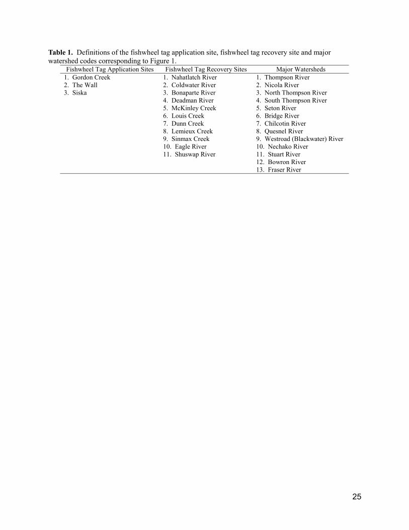
25

Table 1. Definitions of the fishwheel tag application site, fishwheel tag recovery site and majorwatershed codes corresponding to Figure 1.

Fishwheel Tag Application Sites Fishwheel Tag Recovery Sites Major Watersheds1. Gordon Creek 1. Nahatlatch River 1. Thompson River2. The Wall 2. Coldwater River 2. Nicola River3. Siska 3. Bonaparte River 3. North Thompson River

4. Deadman River 4. South Thompson River5. McKinley Creek 5. Seton River6. Louis Creek 6. Bridge River7. Dunn Creek 7. Chilcotin River8. Lemieux Creek 8. Quesnel River9. Sinmax Creek 9. Westroad (Blackwater) River10. Eagle River 10. Nechako River11. Shuswap River 11. Stuart River

12. Bowron River13. Fraser River

26

Table 2. Estimated percentage stock composition, with standard deviations in parentheses, for coho sampled at the Yale andSiska fishwheels.

Fishwheel Sample Size & September October& Year Stock Group 10-16 17-23 24-30 1-7 8-14 15-21 22-28 Total

Siska 2000 n NA 231 100 94 42 252 ND 284Lower Fraser NA 4.4 (3.1) 5.8 (2.9) 3.0 (2.0) 2.5 (4.0) 0.0 (0.0) ND 3.2 (1.6)Thompson NA 95.6 (5.2) 71.7 (5.1) 90.2 (4.0) 93.3 (5.4) 90.8 (7.7) ND 84.1 (3.0)Upper Fraser NA 0.0 (0.7) 15.2 (4.0) 2.9 (2.6) 4.2 (3.1) 5.0 (6.4) ND 7.6 (2.3)Fraser Canyon NA 0.0 (4.8) 7.4 (2.9) 4.0 (2.6) 0.0 (1.3) 4.2 (4.4) ND 5.1 (1.6)

Yale 2000 n 703 83 100 71 47 624 438Lower Fraser 1.7 (2.3) 1.2 (2.1) 0.0 (1.4) 4.5 (3.0) 13.9 (6.6) 12.8 (5.1) 4.1 (1.3)Thompson 76.3 (6.7) 77.0 (6.4) 83.9 (4.6) 74.3 (7.0) 60.1 (9.4) 53.1 (7.1) 73.7 (2.5)Upper Fraser 16.2 (5.0) 19.7 (6.1) 11.3 (4.2) 7.4 (5.3) 13.1 (6.6) 17.6 (6.2) 14.2 (2.4)Fraser Canyon 5.9 (3.6) 2.1 (1.9) 4.9 (2.8) 13.8 (4.9) 12.8 (6.1) 16.6 (5.2) 8.0 (1.7)

Yale 1999 n 975 NA NA NA 97Lower Fraser 2.4 (1.9) NA NA NA 2.4 (1.9)Thompson 83.1 (5.5) NA NA NA 83.1 (5.5)Upper Fraser 11.2 (4.7) NA NA NA 11.2 (4.7)Fraser Canyon 3.3 (2.6) NA NA NA 3.3 (2.6)

Yale 1998 n NA 536 81 127 103 228 271Lower Fraser NA 7.4 (4.1) 4.2 (3.0) 5.4 (9.8) 5.3 (3.0) 14.9 (9.7) 6.3 (1.9)Thompson NA 67.0 (7.6) 65.7 (6.6) 47.7 (16.6) 72.7 (6.4) 60.0 (13.6) 67.7 (4.1)Upper Fraser NA 25.6 (7.2) 14.1 (5.1) 15.9 (11.4) 18.4 (5.3) 19.4 (11.8) 18.2 (3.4)Fraser Canyon NA 0.0 (0.2) 16.0 (5.8) 30.9 (17.1) 3.6 (4.0) 5.6 (8.4) 7.7 (3.0)

NA indicates no samples were collected.ND indicates samples were collected from October 22 to November 3, but could not be analyzed because of problems with thesamples.1. Samples available for September 23 only.2. Samples available for October 18 only.3. Samples available for September 8 to 16.4. Samples available for October 15 to 24.5. Samples available for September 9 to October 36. Samples available for September 21 to 23.7. Samples available for October 2 to 5.8. Samples available for October 15 to November 19.

27

Table 3. Mean bias between trend and true escapement (esc.) estimates for major basins withing theInterior Fraser Management Unit.

North Thompson South Thompson Lower Thompson Fraser1998 1999 2000 98-00 1998 1999 2000 98-00 1998 1999 2000 98-00 1998 1999 2000 98-00

n1 25 29 18 21 24 28 5 6 5 5 5 10True total esc.2 8997 8753 6867 4770 2845 3649 2234 4363 4003 8093 5374 4723Mean bias3 -0.51 -0.48 -0.48 -0.49 -0.35 -0.18 -0.30 -0.28 0.00 -0.04 -0.34 -0.13 -0.57 -0.44 -0.71 -0.571n=number of streams assessed; streams with zero fish counted ignored in mean bias calculation.2Fish taken for brood stock not included in estimates.3Mean bias in escapements between true and trend escapement estimates.

Table 4. Summary of statistical test results for sampling selectivity bias investigations in the application(fishwheels) and recovery (tag recovery sites) samples. Data were stratified by tagging at Yale and Siska.Bias Type Test of Among Yale Siska

Application SampleSpatial Tag incidence Fishwheel tag recovery sites No bias detected Bias high in Lemieux C. and

Shuswap R. and low in McKinleyC. and Bonaparte R.

Temporal Tag incidence Equal recovery periods No bias detected No bias detectedFish Size Size frequency

distributionMarked/unmarked recoveries No bias detected No bias detected

Fish Sex Sex ratio Marked/unmarked recoveries No bias detected Bias toward malesRecovery Sample

Temporal Recovery rate Equal application periods No bias detected No bias detectedFish Size Size frequency

distributionRecovery/not recovered tags No bias detected No bias detected

Fish Sex Sex ratio Recovery/not recovered tags No bias detected No bias detectedFish Stress Recovery rate Active/apparently stressed1 No bias detected No bias detected

1. Apparently stressed fish were lethargic, bleeding, bruised, dropped, or difficult to tag.

28

Table 5. Summary of mark-recapture parameters and pooled Petersen escapement estimates stratified bytagging at Yale and Siska.

Yale SiskaNumber Tagged (M) 667 517Number Examined1 (C) 8,139 7,393Number Recaptured (R) 95 108Tag Incidence (R/C) 1.2% 1.5%Adjusted Tag Rate [(C+1)/(R+1)] 84.8 67.8Petersen Estimate ( talitytaggingmorN %10

ˆ ) 51,000 31,600

95% Confidence Interval 43,300 – 63,400 27,300 – 38,3001. The number examined was higher for Yale than Siska because the Yalerecovery sample included the Siska fishwheel and Nahatlatch Riverlocations.

Table 6. Migration timing reference points from cumulative frequency distributions of the normal curve,Poisson curve, and observed CPUE at the Gordon Creek fishwheel, 2000.

Percentage of the migrationpast Yale

NormalCurve

PoissonCurve

ObservedCPUE

5% September 15 September 13 September 410% September 17 September 15 September 1050% September 24 September 24 September 2390% September 30 October 3 October 595% October 2 October 5 October 9

29

Table 7. Summary estimates of 2000 escapements, fishery mortalities, and exploitations for Thompsonwatershed coho in fisheries in Alaska, North/Central BC, southern BC and Washington.

Number ExploitationSpawning escapement 15300 NAAlaska1 47 0.003North/Central BC1 77 0.005Southern BC

Aboriginal 23 0.002Commercial 8 0.001Recreational 60 0.004Test 49 0.003Experimental 55 0.004

Washington Recreational 60 0.004Aboriginal (treaty) 165 0.011Commercial 0 0.000

Total Canadian 272 0.017Total US 272 0.017TOTAL 544 0.0341Assumed that exploitation rates were the same as computed for 1999.

Table 8. Generational rates of change for escapements of unenhanced coho salmon returning to indicatorstream aggregates in the South and North Thompson drainages.Return Years 1975-2000 1975-1984 1984-1989 1989-1996 1996-2000n1 23 7 3 5 2South Thompson - 16 streams -0.152 0.135 0.114 -0.636 0.378North Thompson - 10 streams -0.030 -0.007 -0.147 -0.483 0.2991n = sum of the generations for each brood line.

Table 9. Summary of provisional reference points for North Thompson coho salmon. See text forexplanation (S = spawners).Model S Females/kmMinimum escapement popn. recovered from 10535 6.1S offset (10% extinction possibility) 7438 4.3

mean 8986 5.2

S MSY 43085 24.9

30

Table 10. Sex ratios for coho returning to streams in the North Thompson watershed1.Dunn Lemieux Louis Mann Sinmax

Ret. Year n % Female n % Female n % Female n % Female n % Female2000 1360 47.4 461 57.5 61 42.6 85 40 96 54.21999 712 48.6 506 47.2 144 43.7 259 48.61998 935 46.6 625 43.7 208 41.2 65 27.71997 331 39.6 367 33.4 123 21.11996 211 48.8 156 40.5 236 21.51995 392 40.3 388 50 446 38.91994 1062 47.6 830 44.1 373 26.31993 587 39.7 564 39.5 290 43.11992 1984 48.2 667 49.3 364 40.41991 1289 46.2 1399 47.5 416 50.71990 772 45.2 592 60.5 109 35.81989 338 57.1 389 51.9 868 45.31988 1497 47.6 430 59.8 467 44.51987 500 45.4 116 49.11986 590 50.5 1041 42.41985 1564 63.7

mean 47.7 47.8 38.1 38.8 54.21 1995-98 Louis and Lemieux data were from Irvine et al. 2000a, other 1985-97 sex ratio data from Irvine et al. 1999a. 1998-99 sex ratio data from Galesloot 1999, 2000 sex ratio data from R. E. Bailey, unpub.

31

0

0

25

40

50miles

80kmKnown Coho Salmon DistributionSuspected Coho Salmon Distribution

Major WatershedsFishwheel Tag Recovery SitesFishwheel Tag Application Sites

.

tr

.

21

3

1

3

6

5

2

4

7

89

10

4

3

1

10

9

8

5

7

6

11

1112 13

2

Fraser Canyon

Figure 1. Known and suspected coho salmon distribution in the interior Fraser River watershed.Numbers for the fishwheel tag application sites, fishwheel tag recovery sites and major watersheds aredefined in Table 1.

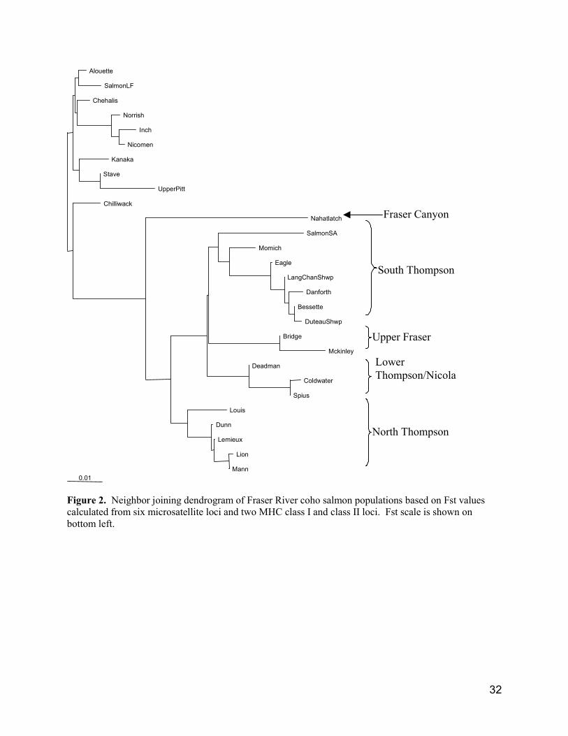
32

LowerThompson/Nicola

0.01

Alouette

SalmonLF

Chehalis

Norrish

Inch

Nicomen

Kanaka

Stave

UpperPitt

Chilliwack

Nahatlatch

SalmonSA

Momich

Eagle

LangChanShwp

Danforth

Bessette

DuteauShwp

Bridge

Mckinley

Deadman

Coldwater

Spius

Louis

Dunn

Lemieux

Lion

Mann

Fraser Canyon

South Thompson

Upper Fraser

North Thompson

Figure 2. Neighbor joining dendrogram of Fraser River coho salmon populations based on Fst valuescalculated from six microsatellite loci and two MHC class I and class II loci. Fst scale is shown onbottom left.

33

Figure 3. Proposed population structure for interior Fraser River coho salmon. *indicates a high degreeof uncertainty. Streams sampled for DNA analysis are listed but not enclosed in boxes.

Nahatlatach

Fraser Canyon

Deadman

LowerThompson

ColdwaterSpius

Nicola

LowerThompsonNicola*

EagleSalmonMomich

Shuswapand Adams Lake

Tributaries

DuteauBessetteDanforth

Lang Channel

ShuswapRiver

Tributaries

SouthThompson

Louis, DunnLion

LemieuxMann

NorthThompson

BridgeMcKinley

Upper Fraser*

InteriorFraserRiver

Watershed

34

0100020003000400050006000

75 77 79 81 83 85 87 89 91 93 95 97 99

Return Year

Num

ber A

dult

Coh

o

Figure 4. Aggregate coho escapement to 10 escapement indicator streams in the North Thompsonwatershed.

0100020003000400050006000

75 77 79 81 83 85 87 89 91 93 95 97 99

Return Year

Num

ber o

f Adu

lt C

oho

Figure 5. Aggregate coho escapement to 16 escapement indicator streams in the South Thompsonwatershed.

35

y = 0.7078x + 849.12R2 = 0.5477

0

1000

2000

3000

4000

5000

6000

0 1000 2000 3000 4000 5000 6000

Index of South Thompson Escapements 1975-2000

Inde

x of

Nor

th T

hom

pson

Esc

apem

ents

197

5-20

00

Figure 6. Relationship between aggregate escapements to South and North Thompson indicator streams.

36

0

5000

10000

15000

20000

25000

30000

75 76 77 78 79 80 81 82 83 84 85 86 87 88 89 90 91 92 93 94 95 96 97 98 99 2000

Return Year

S. a

nd L

. Tho

mps

on

0

20000

40000

60000

80000

100000

120000

N. T

hom

pson

South Thompson Lower Thompson North Thompson

Figure 7. Adjusted historical escapement for coho salmon returning to the North, South, and lower Thompson watersheds (data are in Appendix3).

37

y = 1.3596xR2 = 0.9839

0

5000

10000

15000

20000

25000

30000

0 5000 10000 15000 20000

16 Streams + Eagle and Salmon

Adj

uste

d T

otal

Esc

apem

ents

Figure 8. Relationship between escapements to 16 indicator streams in the South Thompson plusescapements to the Eagle and Salmon rivers and adjusted historical escapements to the South Thompsonwatershed.

y = 13.875xR2 = 0.7719

0

20000

40000

60000

80000

100000

120000

0 1000 2000 3000 4000 5000 6000

10 Stream Index

Adj

uste

d T

otal

Esc

apem

ents

Figure 9. Relationship between escapements to 10 indicator streams in the North Thompson andadjusted historical escapements to the North Thompson watershed.

38

DateDateThe Wall Gordon Creek Siska

0

1

2

3

4

5C

PUE

1998

0

1

2

3

4

5C

PUE

1998

5

0

1

2

3

4

19995

0

1

2

3

4

1999

0

1

2

3

4

5

8-Aug 7-Sep 7-Oct 6-Nov

2000

0

1

2

3

4

5

8-Aug 7-Sep 7-Oct 6-Nov

2000

0

1

2

3

4

5

8-Aug 7-Sep 7-Oct 6-Nov

2000

0

1

2

3

4

5

8-Aug 7-Sep 7-Oct 6-Nov

2000

0

1

2

3

4

5

8-Aug 7-Sep 7-Oct 6-Nov

Date

CPU

E

2000

0

1

2

3

4

5

8-Aug 7-Sep 7-Oct 6-Nov

Date

CPU

E

2000

No Sampling

No Sampling

No Sampling

No Sampling

Figure 10. Migration timing of coho at Yale (the Wall and Gordon Creek) and Siska based on CPUE (fish/hr) at the fishwheels from 1998 to2000. Brackets indicate the seasonal periods of fishwheel operation and the solid line indicates the three-day moving average.

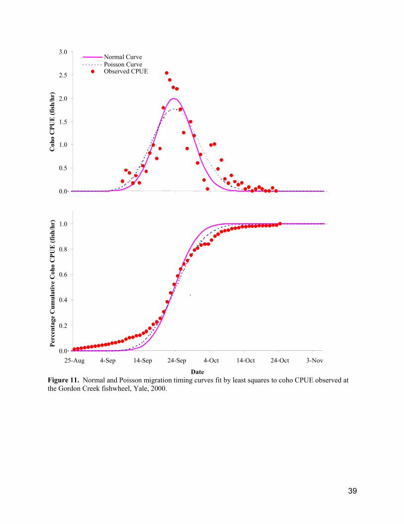
39

0.0

0.2

0.4

0.6

0.8

1.0

25-Aug 4-Sep 14-Sep 24-Sep 4-Oct 14-Oct 24-Oct 3-Nov

Date

Perc

enta

ge C

umul

ativ

e C

oho

CPU

E (f

ish/h

r)

`

0.0

0.5

1.0

1.5

2.0

2.5

3.0C

oho

CPU

E (f

ish/

hr)

Normal CurvePoisson CurveObserved CPUE

Figure 11. Normal and Poisson migration timing curves fit by least squares to coho CPUE observed atthe Gordon Creek fishwheel, Yale, 2000.

40

-1.0-0.50.00.51.01.52.02.5

1978 1983 1988 1993 1998

Return Year

r

Figure 12. Time series of ran, the annual rate of population growth for Thompson coho salmon. Eachpoint is the average (+-SE) of four time series (North and South indicator stream aggregates, Eagle andSalmon rivers). When r<0, populations are unable to replace themselves, even in the absence of fishing.

-2

-1

0

1

2

3

1978 1983 1988 1993 1998

Return Year

r

Figure 13. Time series of ran, the annual rate of population growth of Thompson coho salmon. Eachpoint is the average (+-SE) of two time series (North and South indicator stream aggregates). When r<0,populations are unable to replace themselves, even in the absence of fishing.

41

-0.05

0.15

0.35

0.55

0.75

0.95

1987 1992 1997Return Year

Expl

oita

tion

Rat

e

Figure 14. Exploitation rate estimates for Thompson watershed (North and South indicator streamaggregates, Eagle and Salmon rivers) coho (solid line) and exploitation rates that would have maintainedcoho production at the brood year escapement level (i.e. St = St-3 ) (dashed line).

-0.05

0.15

0.35

0.55

0.75

0.95

1987 1992 1997Return Year

Expl

oita

tion

Rat

e

Figure 15. Exploitation rate estimates for Thompson watershed (North and South indicator streamaggregates) coho (solid line) and exploitation rates that would have maintained coho production at thebrood year escapement level (i.e. St = St-3 ) (dashed line).

42

0

10

20

30

40

50

60

75 76 77 78 79 80 81 82 83 84 85 86 87 88 89 90 91 92 93 94 95 96 97 98 99

2000

Return Year

Fem

ale

Coho

Spa

wne

rs p

er K

ilom

etre

of A

cces

sibl

e Ha

bita

t

Figure 16. Annual estimates of numbers of female coho per kilometre within the North Thompsonwatershed. Horizontal line indicates the mean of two possible limit reference points (5.2 females/km).

43

Appendix 1. Coho DNA mixed stock estimates for 1997-1999 sampling, N= number of fish in sample. Standard deviations are in brackets. Samples with *indicates 1998 and 1999 samples analyzed in year 2000. Thompson and Upper Fraser combined for 1997 and 1998 samples analyzed in 1998.

Southern BaselineArea20 Seine Test Fishery

1998 1999 1998 1999 1998 1999 1998 1999 1998 1999 1998 1999July 24-25 July 21-24 July 26-Aug 1 July 25-31 Aug 2 - 8 Aug 1-3 Aug 9 -15 Aug 8-14 Aug 16- 22 Aug 15-21 Aug 23-25 Aug 22-28

N 184 172 310 252 153 50 168 99 155 207 59 63WCVI 14.2 (3.4) 7.2 (2.9) 3.9 (2.5) 1.7 (1.2) 5.4 (3.4) 1.7 (1.2) 9.3 (3.8) 4.5 (3.8) 6.7 (3.5) 3.9 (1.9) 8.9 (5.4) 7.4 (5.3)ECVI 9.3 (3.7) 4.5 (3.0) 8.4 (2.8) 12.6 (3.2) 4.6 (3.0) 12.6 (3.2) 17.6 (5.8) 22.3 (5.8) 6.7 (3.9) 19.6 (3.9) 12.5 (7.8) 20.2 (9.3)NCVI 1.3 (2.2) 2.3 (2.3) 6.8 (2.0) 6.0 (2.1) 0.9 (2.2) 6.0 (2.1) 1.3 (1.7) 0.0 (2.2) 3.3 (2.1) 1.4 (1.7) 4.6 (4.2) 4.7 (4.3)S. Mainland 10.2 (3.2) 10.3 (3.1) 7.0 (2.3) 14.9 (2.7) 12.4 (4.7) 14.9 (2.7) 7.5 (3.7) 7.4 (4.9) 4.2 (3.1) 9.5 (2.9) 5.0 (5.4) 25.9 (7.6)Lower Fraser 15.7 (4.2) 23.9 (4.5) 13.2 (3.0) 14.7 (3.3) 9.7 (4.4) 14.7 (3.3) 3.3 (3.4) 13.9 (5.2) 4.9 (3.3) 14.3 (3.5) 1.1 (3.3) 10.1 (6.5)Thompson/UPFR 1.3 (1.3) 0.8 (0.7) 2.8 (1.4) 1.4 (1.1) 1.1 (0.9) 2.3 (2.2)Thompson 1.3 (0.9) 0.0 (0.5) 0.0 (0.5) 1.9 (1.8) 1.9 (1.1) 0.0 (0.8)UPFR 0.0 (0.2) 0.0 (0.2) 0.0 (0.2) 0.0 (0.4) 0.7 (1.1) 0.0 (0.5)Puget S. 36.5 (4.7) 39.8 (5.2) 36.2 (4.5) 37.9 (4.5) 39.6 (6.7) 37.9 (4.5) 41.2 (5.1) 29.3 (6.6) 32.3 (6.4) 41.4 (4.6) 47.8 (8.7) 25.9 (8.7)Juan de Fuca 4.0 (3.3) 5.6 (2.9) 12.6 (3.5) 2.9 (2.0) 17.3 (5.2) 2.9 (2.0) 5.4 (3.6) 10.7 (5.0) 18.4 (5.7) 1.9 (1.9) 7.2 (4.8) 0.0 (2.3)Coastal Wash 4.1 (2.2) 2.1 (1.8) 9.5 (2.8) 4.3 (1.9) 1.1 (2.8) 4.3 (1.9) 8.8 (2.8) 8.7 (4.8) 18.3 (4.4) 1.9 (1.4) 8.4 (5.2) 0.0 (2.9)Columbia 3.4 (1.5) 2.9 (1.6) 1.7 (1.2) 5.0 (1.9) 6.3 (2.3) 5.0 (1.9) 4.2 (1.9) 1.4 (2.0) 4.2 (2.1) 3.5 (1.5) 2.4 (2.2) 5.9 (3.2)

{Canada 52.1 (5.0) 49.5 (5.6) 40.1 (4.2) 49.9 (4.8) 35.7 (6.7) 49.9 (4.8) 40.4 (5.7) 49.9 (7.4) 26.8 (5.5) 51.3 (4.4) 34.3 (9.3) 68.2 (9.0){US 47.9 (5.0) 50.5 (5.6) 59.9 (4.2) 50.1 (4.8) 64.3 (6.7) 50.1 (4.8) 59.6 (5.7) 50.1 (7.4) 73.2 (5.5) 48.7 (4.4) 65.7 (9.3) 31.8 (9.0)

Area 20 Gillnet Test Fishery1998 1999 1998 1999 1988 1999 1998

July 3-18 July 14-17 July 19-25 July18-24 July 26-Aug 1 July 25-31 Aug 2-16N 123 111 22 116 85 58 66WCVI 21.2 (5.2) 8.0 (3.9) 17.4 (9.0) 0.0 (1.5) 18.5 (6.4) 6.5 (5.5) 15.4 (6.7)ECVI 6.9 (3.8) 14.2 (5.8) 4.7 (8.0) 12.3 (6.1) 12.1 (6.1) 15.6 (8.7) 4.3 (4.2)NCVI 3.6 (3.1) 6.4 (3.7) 1.7 (4.6) 2.0 (2.2) 7.4 (4.5) 9.5 (6.5) 8.2 (5.9)S. Mainland 9.5 (4.4) 7.7 (4.9) 13.8 (8.8) 15.9 (5.2) 9.8 (4.7) 4.8 (5.3) 16.0 (6.7)Lower Fraser 7.5 (3.6) 22.0 (5.4) 0.0 (7.3) 15.3 (5.7) 4.2 (5.7) 17.1 (9.3) 5.5 (7.4)Thompson/UPFR 1.0 (0.8) 0.0 (0.0) 1.3 (1.6) 0.0 (0.6)Thompson 2.1 (1.4) 0.4 (1.5) 1.1 (1.8)UPFR 0.0 (0.4) 1.6 (1.5) 0.0 (0.0)Puget S. 24.4 (5.8) 31.4 (6.9) 8.1 (11.2) 41.3 (6.6) 15.4 (6.6) 40.8 (10.4) 14.2 (7.2)Juan de Fuca 4.6 (3.3) 2.8 (3.2) 31.9 (13.4) 4.9 (3.7) 14.4 (6.2) 1.7 (3.2) 14.5 (7.7)Coastal Wash 13.1 (4.4) 5.6 (3.1) 22.4 (14.1) 5.2 (3.7) 9.2 (3.9) 0.0 (2.8) 20.6 (6.4)Columbia 8.3 (3.1) 0.0 (0.8) 0.0 (0.6) 1.3 (1.5) 7.7 (4.1) 2.9 (2.7) 1.4 (2.6)

{Canada 49.6 (5.5) 60.3 (7.0) 37.7 (13.5) 47.4 (6.5) 53.3 (8.2) 54.6 (11.0) 49.3 (9.3){US 50.4 (5.5) 39.7 (7.0) 62.3 (13.5) 52.6 (6.5) 46.7 (8.2) 45.4 (11.0) 50.7 (9.3)

44

Appendix 1 - cont.

Gillnet Seine Washington Troll Fishery1999 1998* 1998 1998 1999 1998* 1999 1999 1999 1999 1999

Wash A5 Area14 Area21 Area23 Area20 Area 21 Area 3 Area 4 Area 4 Area 4 Area 4/4bAug 4-5 Nov2-10 Oct 17-24 Sept 9-11 Aug 6 Oct 11-12 Aug15-18 < Aug 15 Aug 16-31 Sept 2 Aug 22

N 44 6 153 100 122 35(35) 56 101 180 199 207WCVI 12.1 (6.0) 16.2 (9.6) 38.2 (6.5) 89.2 (5.4) 2.3 (2.6) 60.9 (11.9) 9.1 (5.4) 0.1 (2.6) 6.8 (3.5) 4.4 (2.6) 2.5 (2.7)ECVI 6.8 (7.2) 13.0 (18.6) 18.8 (4.6) 6.5 (3.7) 12.5 (6.1) 3.0 (4.6) 3.6 (5.0) 9.1 (4.0) 7.0 (3.7) 11.1 (4.6) 0.0 (2.2)NCVI 0.0 (3.9) 0.0 (14.9) 3.6 (3.0) 2.9 (2.9) 1.2 (2.3) 0.0 (7.6) 5.4 (4.6) 2.4 (2.3) 0.7 (1.6) 0.7 (2.3) 4.2 (2.2)S. Mainland 16.6 (8.3) 17.8 (15.6) 16.9 (5.1) 0.0 (1.2) 10.4 (5.3) 9.3 (6.5) 3.9 (4.1) 1.5 (2.4) 2.9 (2.6) 1.2 (2.9) 11.1 (3.2)Lower Fraser 19.9 (7.8) 15.6 (25.8) 5.8 (3.2) 1.5 (1.6) 26.1 (6.7) 15.8 (7.8) 4.4 (4.0) 15.1 (5.1) 10.5 (4.3) 21.6 (4.3) 12.8 (3.5)Thompson/UPFR 1.2 (1.1) 0.0 (0.4)Thompson 4.9 (3.5) 0.0 (0.0) 1.3 (1.7) 0.0 (0.0) 3.2 (2.6) 5.5 (2.9) 4.4 (2.1) 3.0 (1.6) 1.2 (1.2)UPFR 0.0 (0.0) 0.0 (0.0) 0.0 (0.0) 0.0 (0.0) 1.4 (1.1) 1.1 (0.9) 0.0 (0.2) 0.0 (0.5) 0.0 (0.3)Puget S. 37.1 (10.3) 17.1 (15.6) 6.9 (4.1) 0.0 (2.1) 34.1 (7.9) 1.5 (5.7) 19.6 (9.3) 44.9 (7.0) 25.5 (6.1) 29.5 (4.8) 30.6 (4.8)Juan de Fuca 2.6 (3.6) 0.0 (9.1) 0.1 (2.6) 0.0 (1.7) 8.8 (4.3) 7.7 (4.4) 0.0 (2.1) 3.0 (3.8) 11.9 (4.1) 1.7 (1.9) 1.6 (2.4)Coastal Wash 0.0 (1.8) 20.4 (20.9) 8.5 (4.2) 0.0 (1.2) 1.9 (3.8) 1.7 (4.3) 29.4 (9.1) 12.8 (4.9) 17.2 (5.6) 20.8 (4.7) 22.7 (4.2)Columbia 0.0 (2.2) 0.0 (8.4) 0.0 (1.0) 0.0 (0.5) 1.4 (2.3) 0.0 (1.6) 20.0 (6.6) 4.5 (2.6) 13.0 (3.1) 6.0 (2.9) 13.3 (2.9)

{Canada 60.3 (10.9) 62.6 (23.4) 84.5 (5.7) 100.0 (3.0) 53.9 (7.7) 89.1 (7.2) 30.9 (9.2) 34.8 (7.0) 32.4 (5.2) 42.0 (6.2) 31.7 (4.9){US 39.7 (10.9) 37.4 (23.4) 15.5 (5.7) 0.0 (3.0) 46.1 (7.7) 10.9 (7.2) 69.1 (9.2) 65.2 (7.0) 67.6 (5.2) 58.0 (6.2) 68.3 (4.9)

Canadian Troll Fishery Recreational Fishery1999 1999 1999 1998 1998 1998 1997 1997 1998 1999

Area 123 Area 123 Area 123 Area 14 Area 17 Area 19 Area 20 Area 20 Area 20 Area20

Port Renfrew Port Renfrew

July 25-31 Aug 12-13 Sept2-14 Oct 2-29 July 29-31 Jul5-Sep27 Aug1-24 Aug24-Sept5 July 26-Sept 9 Aug 8-13N 194 204 211 67 12 73 77 77 46 81WCVI 4.4 (2.3) 1.7 (2.3) 7.5 (2.6) 0.2 (1.9) 7.5 (10.4) 12.6 (7.2) 7.9 (4.9) 6.4 (6.1) 18.1 (8.1) 1.5 (2.4)ECVI 9.6 (3.6) 7.6 (2.8) 12.3 (3.9) 84.7 (6.6) 16.5 (10.7) 9.5 (6.2) 4.1 (5.3) 22.2 (7.4) 9.5 (6.0) 14.2 (7.8)NCVI 1.5 (1.5) 3.1 (2.3) 3.4 (2.5) 2.7 (2.4) 0.0 (0.6) 5.8 (4.7) 0.9 (3.2) 8.8 (5.1) 11.2 (6.5) 7.3 (4.0)S. Mainland 7.9 (2.9) 5.9 (2.3) 7.0 (2.9) 6.3 (5.8) 0.0 (9.1) 24.0 (8.5) 1.6 (3.6) 7.3 (6.3) 15.6 (6.9) 12.8 (4.8)Lower Fraser 24.3 (4.2) 23.6 (3.7) 32.2 (4.1) 0.0 (1.4) 45.0 (16.9) 10.1 (5.4) 37.3 (8.5) 18.0 (7.1) 11.0 (4.5) 14.2 (6.0)Thompson/UPFR 0.0 (0.0) 8.3 (7.5) 3.8 (3.0) 3.7 (2.5) 5.8 (2.8) 6.3 (4.6)Thompson 3.3 (1.5) 2.2 (1.2) 0.5 (0.6) 1.2 (1.1)UPFR 0.0 (0.6) 0.6 (0.6) 0.0 (0.4) 0.0 (0.0)Puget S. 27.4 (4.6) 36.9 (4.2) 22.0 (3.4) 0.0 (1.6) 22.7 (11.9) 26.3 (7.5) 31.1 (9.8) 12.3 (7.0) 9.4 (6.7) 33.7 (7.9)Juan de Fuca 13.2 (3.8) 8.0 (2.4) 4.2 (2.9) 0.8 (1.7) 0.0 (2.5) 4.4 (3.9) 10.4 (6.5) 6.0 (4.1) 7.3 (5.2) 5.9 (4.6)Coastal Wash 8.0 (2.5) 6.6 (3.0) 7.1 (2.5) 5.2 (3.3) 0.0 (3.1) 3.6 (4.4) 3.0 (3.8) 9.2 (4.3) 6.4 (4.6) 4.8 (3.8)Columbia 0.3 (0.8) 3.6 (1.7) 3.8 (1.6) 0.0 (0.0) 0.0 (0.0) 0.0 (0.4) 0.0 (1.3) 4.0 (3.1) 5.2 (3.4) 4.5 (2.7)

{Canada 51.2 (5.0) 44.8 (4.4) 62.9 (4.3) 94.0 (4.0) 77.3 (12.4) 65.7 (8.1) 55.5 (8.8) 68.5 (8.4) 71.7 (8.9) 51.1 (8.2){US 48.8 (5.0) 55.2 (4.4) 37.1 (4.3) 6.1 (4.0) 22.7 (12.4) 34.3 (8.1) 44.5 (8.8) 31.5 (8.4) 28.3 (8.9) 48.9 (8.2)

45

Appendix 1 – cont.Recreational Fisheries

1999 1999 1997 1998 1999 1997 1999 1998 1998 1999 1998 1998 1998Area 20 Area 20 Area 23 Area 23 Area 23 Area 23 Area 23 Area28 Area 29 Area 123/124 US Area 5 US Area 5 US Area 5Guides BCWF Ucluelet Ucluelet Ucluelet Bamfield Bamfield

Aug10-Oct1 Aug 15-Sept5 July 12-19 Aug1-Sept9 July7-Sept11 July 20-30 July31-Aug16 July1-16 July15-Oct19 Aug16-Sept1 Aug-16 Aug23 Sept 05N 18 59 86 14 115 63 247 42 17 31 147 149 146WCVI 14.9 (11.4) 2.7 (3.0) 16.3 (6.1) 52.5 (17.5) 29.5 (5.7) 15.0 (6.0) 87.3 (3.5) 4.2 (6.9) 13.3 (12.2) 14.6 (6.7) 8.7 (4.1) 2.9 (2.5) 3.4 (2.8)ECVI 3.5 (9.3) 16.8 (6.3) 4.9 (5.0) 0.0 (8.9) 16.0 (5.4) 5.7 (4.5) 2.8 (1.8) 0.0 (3.3) 5.3 (10.8) 14.6 (6.6) 6.2 (3.9) 10.1 (3.8) 2.6 (3.4)NCVI 0.0 (5.8) 5.5 (4.2) 2.1 (3.0) 14.6 (9.8) 10.4 (4.2) 3.0 (3.3) 1.6 (2.3) 0.0 (1.1) 0.0 (3.8) 2.5 (4.2) 5.5 (2.8) 7.4 (3.1) 0.7 (1.4)S. Mainland 16.5 (11.9) 11.4 (6.2) 5.0 (4.1) 17.5 (14.4) 6.9 (3.6) 3.6 (4.2) 4.2 (2.1) 65.2 (15.5) 35.8 (17.3) 5.6 (5.3) 6.2 (3.8) 4.0 (2.9) 8.5 (4.3)Lower Fraser 30.9 (14.8) 13.6 (6.2) 30.4 (7.2) 7.6 (7.8) 15.9 (5.2) 12.3 (6.7) 2.4 (1.6) 0.0 (7.0) 14.9 (12.6) 26.1 (10.9) 7.9 (4.5) 9.3 (3.0) 5.8 (2.4)Thompson/UPFR 1.1 (1.5) 0.0 (0.0) 2.4 (2.2) 2.23 2.01 6.0 (6.9) 1.1 (0.9) 1.1 (1.2) 4.6 (1.7)Thompson 0.0 (0.0) 6.7 2.94 4.8 (2.2) 0.0 (0.4) 0.0 (3.3)UPFR 0.0 (0.0) 1.8 (2.0) 0.0 (0.1) 0.0 (0.3) 0.0 (0.0)Puget S. 20.7 (10.4) 37.5 (8.2) 22.0 (7.0) 7.8 (8.1) 5.4 (2.9) 39.1 (8.1) 1.2 (1.1) 4.08 6.23 0.0 (5.4) 13.6 (7.3) 43.1 (6.8) 45.4 (5.8) 59.4 (6.3)Juan de Fuca 5.5 (7.6) 0.0 (2.4) 6.4 (5.2) 0.0 (1.8) 2.9 (2.1) 6.4 (4.2) 0.0 (0.6) 0.0 (0.3) 0.0 (0.0) 0.0 (1.7) 3.5 (3.3) 5.8 (3.5) 7.2 (3.8)Coastal Wash 5.2 (6.5) 4.0 (3.5) 6.2 (4.6) 0.0 (3.3) 8.3 (3.7) 10.4 (5.9) 0.2 (0.8) 22.7 (12.9) 12.0 (14.7) 19.9 (7.4) 15.1 (3.8) 6.7 (4.3) 4.4 (2.5)Columbia 2.8 (4.2) 0.0 (1.8) 5.5 (3.2) 0.0 (0.0) 0.0 (0.7) 2.0 (1.9) 0.3 (0.4) 1.6 (6.4) 12.7 (12.2) 3.2 (3.0) 2.7 (1.6) 7.1 (2.8) 3.3 (2.0)

0.0 (0.0){Canada 65.8 (11.3) 58.5 (7.7) 59.9 (9.0) 92.2 (8.4) 83.4 (4.7) 42.2 (8.6) 98.2 (1.5) 71.7 (13.5) 75.3 (15.4) 63.3 (10.4) 35.6 (6.2) 34.9 (5.2) 25.6 (5.1){US 34.2 (11.3) 41.5 (7.7) 40.1 (9.0) 7.8 (8.4) 16.6 (4.7) 57.8 (8.6) 1.8 (1.5) 28.3 (13.5) 24.7 (15.4) 36.7 (10.4) 64.4 (6.2) 65.1 (5.2) 74.4 (5.1)

Central BaselineSeine Fisheries Round Isl Test Seine Seized

1998 1998* 1998* 1998* 1998 1998* 1998* 1998* 1998 1998 1998 1998 1999Area 12 Area 12 Area 12 Area 12 Area 13 Area 13 Area 13 Area 13 Area 12 Area 12 Area7 Area8 Area8/9Aug3-26 Oct10-13 Oct17-22 Oct 23-24 Aug3-8 Oct14-17 Oct 19-23 Nov1-13 July 16-31 Aug 1-13 Aug30-Sept12 Jul18-Aug29 Aug 13 - Oct

24N 108 49 87 36(36) 18 161 112 118 59 27 22 131 40QCI 2.9 (2.0) 0.0 (1.1) 1.3 (1.5) 5.0 (4.2) 0.0 (5.2) 1.1 (1.8) 1.6 (1.4) 0.0 (0.7) 6.9 (4.0) 2.7 (4.8) 0.0 (1.3) 2.3 (1.7) 5.1 (4.6)Nass 0.0 (1.6) 0.0 (0.8) 0.0 (1.7) 3.5 (3.2) 0.0 (2.7) 0.0 (1.4) 0.0 (0.4) 0.0 (1.0) 0.0 (1.6) 0.0 (1.8) 0.0 (1.9) 1.9 (1.7) 0.0 (1.0)Upper Skeena 1.7 (1.7) 0.0 (2.0) 1.0 (1.4) 0.0 (0.8) 0.0 (4.5) 1.3 (1.6) 0.0 (0.3) 2.0 (1.5) 5.1 (3.1) 0.0 (2.8) 0.0 (3.4) 0.0 (0.6) 0.0 (1.3)Lower Skeena 0.0 (2.2) 0.0 (2.7) 3.0 (2.9) 1.8 (4.1) 6.4 (6.2) 0.5 (1.9) 0.7 (2.5) 3.0 (2.4) 9.5 (4.5) 3.9 (5.4) 8.6 (7.9) 4.2 (2.7) 2.8 (3.7)North/Central Coast 17.5 (7.4) 7.1 (6.0) 14.4 (6.8) 1.2 (5.3) 20.1 (12.7) 9.1 (3.2) 1.4 (3.7) 1.2 (2.4) 16.5 (7.1) 14.7 (7.5) 37.6 (15.3) 69.6 (6.7) 28.9 (9.1)WCVI 7.3 (4.0) 11.2 (5.1) 4.1 (3.3) 8.1 (4.6) 0.0 (7.5) 3.5 (3.4) 5.0 (3.6) 6.0 (3.8) 11.1 (6.9) 21.9 (11.4) 13.4 (10.0) 10.7 (3.8) 7.2 (7.1)ECVI 15.7 (6.3) 42.1 (10.4) 30.1 (7.1) 44.1 (11.7) 30.1 (14.4) 30.6 (7.0) 32.0 (6.2) 40.7 (6.6) 10.5 (6.4) 11.0 (9.8) 0.0 (5.4) 2.2 (3.1) 10.0 (6.5)NCVI 8.2 (3.9) 2.2 (3.1) 8.2 (5.8) 6.3 (6.0) 0.0 (3.6) 2.0 (2.6) 4.7 (3.1) 0.9 (2.7) 15.3 (5.8) 11.0 (7.1) 35.0 (13.2) 2.0 (2.3) 9.2 (6.1)South Main 25.1 (7.7) 11.9 (9.1) 5.9 (5.3) 0.0 (3.0) 18.1 (12.1) 12.4 (4.6) 13.4 (5.2) 7.9 (3.9) 11.7 (5.2) 0.0 (3.7) 0.5 (9.2) 5.6 (4.0) 15.0 (7.6)Lower Fraser 7.1 (3.0) 9.5 (7.2) 21.0 (5.6) 13.1 (6.4) 4.0 (7.8) 28.3 (6.1) 28.2 (5.8) 26.5 (6.2) 2.1 (3.0) 7.8 (6.3) 5.0 (6.3) 0.0 (0.9) 5.8 (5.1)Thompson/UPFR 2.6 (1.5) 5.6 (5.0) 0.0 (0.0) 0.0 (0.0) 0.0 (2.5) 0.0 (0.5)Thompson 1.4 (2.4) 0.0 (1.1) 7.7 (3.9) 1.0 (1.2) 0.4 (1.1) 0.0 (0.6) 0.0 (0.0)UPFR 3.1 (3.3) 1.2 (1.2) 3.0 (5.0) 0.0 (0.5) 2.7 (1.7) 0.0 (0.7) 0.0 (0.0)Puget Sound 9.0 (4.2) 7.4 (6.8) 3.7 (3.5) 0.0 (2.9) 15.8 (10.0) 8.6 (4.5) 5.4 (4.1) 6.6 (4.6) 9.1 (4.8) 14.0 (9.0) 0.0 (0.0) 0.0 (1.1) 10.2 (5.9)Juan de Fuca 3.2 (2.8) 0.0 (2.4) 0.5 (2.6) 6.1 (5.9) 0.0 (0.0) 0.0 (1.7) 1.6 (1.5) 0.7 (2.0) 0.0 (1.2) 0.0 (1.1) 0.0 (5.0) 1.5 (1.5) 0.0 (1.6)Coastal Wash 0.0 (2.5) 4.1 (5.5) 3.5 (2.5) 0.0 (2.2) 0.0 (0.0) 1.8 (2.5) 0.7 (1.4) 2.1 (1.9) 0.0 (3.0) 5.8 (6.9) 0.0 (0.0) 0.0 (0.9) 3.6 (2.7)Columbia 0.0 (0.2) 0.0 (2.3) 2.1 (1.8) 0.0 (1.6) 0.0 (3.8) 0.0 (0.8) 2.1 (1.9) 2.5 (1.9) 2.3 (1.9) 7.3 (4.9) 0.0 (0.0) 0.0 (0.4) 2.2 (1.6)

0.0 (0.0){Canada 87.8 (4.6) 88.5 (7.9) 90.2 (5.0) 93.9 (6.8) 84.2 (10.0) 89.6 (5.2) 90.1 (4.7) 88.2 (5.1) 88.7 (6.1) 72.9 (8.8) 100.0 (5.1) 98.5 (2.0) 84.0 (6.7){U.S. 12.2 (4.6) 11.5 (7.9) 9.8 (5.0) 6.1 (6.8) 15.8 (10.0) 10.4 (5.2) 9.9 (4.7) 11.8 (5.1) 11.3 (6.1) 27.1 (8.8) 0.0 (5.1) 1.5 (2.0) 16.1 (6.7)

46

Appendix 1 – cont.Gillnet Troll Fishery

1998 1999* 1998 1999 1998 1999* 1999* 1999* 1999* 1999*Area 12 Area12 Area 11 Area 11 Area 12 Area12 Area12 Area12 Area12 Area13

Aug26-30 Jul24-Aug5 July 26-Aug8 Aug 3 July 24-31 Jul01 Jul11 Jul18-19 Jul24-Oct17 Aug6-Sep29N 27 65(65) 47 23 196 52(52) 43(43) 268(268) 13(13) 65(65)QCI 0.0 (8.2) 0.0 (2.0) 7.8 (4.2) 2.7 (4.3) 0.3 (1.1) 1.5 (2.5) 0.0 (1.9) 2.2 (1.6) 0.0 (6.1) 0.0 (1.0)Nass 2.9 (4.8) 1.8 (1.8) 0.0 (3.6) 4.4 (4.8) 1.4 (1.9) 0.0 (0.4) 1.5 (2.3) 0.8 (1.4) 0.2 (6.2) 0.0 (4.5)Upper Skeena 0.0 (2.9) 0.0 (1.2) 3.9 (3.4) 0.0 (1.2) 1.0 (0.9) 0.0 (0.5) 0.0 (1.7) 0.5 (0.9) 8.9 (10.4) 3.1 (2.3)Lower Skeena 3.3 (7.4) 0.0 (2.0) 9.8 (5.4) 4.4 (5.8) 1.6 (1.4) 5.1 (4.5) 2.7 (2.4) 1.6 (1.9) 0.0 (5.0) 7.9 (6.1)North/Central Coast 33.9 (13.2) 17.7 (8.4) 19.9 (7.6) 33.6 (12.5) 7.0 (3.9) 11.7 (5.4) 8.9 (8.1) 26.4 (4.5) 47.9 (21.7) 14.4 (6.7)WCVI 18.0 (12.2) 2.3 (5.9) 7.5 (6.3) 11.3 (9.0) 16.3 (4.8) 15.7 (5.9) 13.4 (7.6) 5.8 (2.7) 0.9 (8.4) 8.0 (4.8)ECVI 19.6 (13.2) 12.1 (9.1) 12.8 (6.8) 2.2 (3.9) 24.6 (5.3) 33.1 (7.8) 37.2 (10.9) 21.9 (4.0) 28.3 (14.0) 9.7 (6.0)NCVI 7.9 (9.0) 16.2 (6.2) 9.6 (6.2) 15.5 (10.9) 8.5 (3.2) 2.2 (3.4) 12.5 (6.9) 15.1 (3.4) 0.1 (6.9) 1.8 (2.9)South Main 6.5 (7.9) 28.8 (8.3) 0.4 (4.1) 4.9 (7.1) 18.0 (5.9) 16.1 (6.7) 6.4 (5.9) 8.0 (3.2) 0.0 (11.3) 39.8 (10.6)Lower Fraser 0.0 (5.8) 12.2 (7.0) 14.8 (6.2) 3.8 (5.7) 5.4 (2.9) 8.4 (5.8) 6.4 (6.0) 7.2 (2.9) 0.0 (4.1) 8.5 (5.3)Thompson/UPFR 0.4 (3.8) 2.3 (2.2) 3.0 (1.3)Thompson 0.0 (0.6) 8.1 (5.8) 1.8 (1.8) 0.0 (0.4) 0.7 (0.5) 0.0 (0.0) 2.1 (2.4)UPFR 0.3 (2.3) 0.0 (1.0) 0.0 (0.8) 0.0 (0.1) 0.2 (0.6) 4.8 (6.6) 0.9 (1.1)Puget Sound 7.7 (7.7) 6.5 (4.7) 3.4 (3.7) 0.0 (1.7) 8.8 (4.0) 2.0 (3.3) 5.3 (3.1) 7.7 (2.4) 0.9 (9.0) 0.0 (3.6)Juan de Fuca 0.0 (4.1) 2.3 (4.3) 3.1 (3.0) 3.4 (3.4) 1.9 (1.7) 0.0 (0.2) 0.0 (2.5) 1.4 (1.6) 8.0 (8.8) 0.0 (2.2)Coastal Wash 0.0 (3.0) 0.0 (1.8) 4.8 (4.4) 0.0 (0.0) 0.7 (1.2) 2.4 (3.5) 0.0 (1.7) 0.4 (1.0) 0.0 (1.4) 1.9 (2.6)Columbia 0.0 (1.2) 0.0 (1.8) 0.0 (0.7) 5.7 (5.5) 1.6 (1.3) 0.0 (1.8) 5.8 (4.0) 0.1 (1.2) 0.0 (3.2) 2.1 (2.2)

{Canada 92.3 (8.7) 91.2 (6.1) 88.8 (5.8) 90.9 (6.6) 87.0 (4.4) 95.6 (4.7) 88.9 (5.5) 90.4 (2.9) 91.2 (12.4) 96.0 (5.2){U.S. 7.7 (8.7) 8.8 (6.1) 11.3 (5.8) 9.1 (6.6) 13.0 (4.4) 4.4 (4.7) 11.1 (5.5) 9.6 (2.9) 8.8 (12.4) 4.0 (5.2)

Troll Fisheries1998 1998 1998 1999 1999 1998 1999 1999 1999 1999 1998

Area 12 Area 12 Area 12 Area 12 Area124 Area124 Area124 Area124 Area124 Area125 Area125Aug 1-7 Aug 8-16 Aug 17-25 July 23-Aug6 Jul23-31 Aug1-7 Aug1-7 Aug8-14 Sept12-15 Jul25-31 Aug1-7

N 68 292 44 158 260 55 110 199 191 264 260QCI 2.6 (2.4) 1.6 (0.8) 1.4 (2.8) 0.9 (1.4) 0.8 (1.0) 1.5 (1.8) 0.0 (1.0) 0.3 (1.4) 1.5 (1.5) 0.8 (0.8) 1.3 (1.3)Nass 1.7 (3.0) 0.0 (1.4) 0.0 (1.0) 0.0 (1.0) 0.0 (0.8) 0.0 (1.0) 1.2 (1.1) 0.0 (0.5) 0.3 (1.0) 0.3 (0.7) 1.2 (1.2)Upper Skeena 1.6 (2.5) 0.3 (0.5) 0.0 (0.7) 0.0 (0.7) 0.9 (0.7) 0.0 (0.2) 0.5 (1.3) 0.0 (0.7) 0.0 (0.3) 0.7 (0.8) 0.0 (0.6)Lower Skeena 5.2 (3.6) 5.1 (2.5) 1.7 (3.6) 1.4 (1.8) 3.0 (1.8) 2.7 (3.2) 0.2 (1.5) 4.3 (2.2) 0.2 (0.9) 2.6 (1.9) 1.0 (1.0)North/Central Coast 6.5 (5.0) 19.8 (3.8) 0.0 (6.6) 23.7 (4.9) 9.7 (2.7) 3.3 (2.8) 6.0 (3.1) 7.5 (2.9) 2.8 (1.9) 2.1 (1.9) 3.3 (2.1)WCVI 10.4 (6.5) 14.4 (4.8) 4.8 (6.9) 19.3 (5.1) 19.2 (3.4) 26.8 (6.9) 25.5 (4.9) 20.4 (4.4) 33.2 (5.0) 18.6 (3.3) 23.7 (4.0)ECVI 21.8 (8.5) 4.1 (2.9) 22.7 (7.7) 11.1 (3.9) 11.9 (3.6) 0.0 (3.2) 1.9 (3.8) 11.8 (3.2) 17.5 (4.8) 13.3 (3.3) 12.2 (3.9)NCVI 18.7 (7.4) 18.8 (3.3) 24.7 (8.2) 10.9 (4.4) 8.5 (2.7) 8.6 (5.7) 4.1 (3.4) 6.0 (2.7) 9.3 (3.6) 5.5 (2.2) 7.1 (3.1)South Main 12.4 (6.3) 14.9 (3.8) 9.3 (6.0) 20.0 (5.6) 3.6 (2.2) 5.8 (4.0) 2.8 (2.2) 0.0 (1.3) 5.6 (2.9) 5.7 (2.4) 2.6 (2.0)Lower Fraser 12.5 (6.1) 3.2 (1.9) 17.2 (6.8) 5.3 (2.8) 19.9 (3.4) 16.0 (7.2) 17.1 (5.0) 20.1 (3.8) 13.8 (3.5) 24.8 (3.3) 12.3 (3.2)Thompson/UPFR 2.1 (1.6) 2.3 (1.0) 2.3 (2.9) 1.0 (1.3) 2.3 (1.2)Thompson 0.0 (0.5) 1.2 (1.0) 0.9 (1.7) 0.6 (0.6) 0.6 (0.7) 0.9 (0.9)UPFR 0.0 (0.1) 1.5 (0.9) 1.5 (1.1) 0.5 (0.5) 0.0 (0.2) 1.5 (1.0)Puget Sound 3.8 (3.8) 7.5 (2.5) 7.3 (4.9) 1.6 (1.8) 12.0 (3.5) 13.9 (7.8) 19.2 (4.9) 16.6 (3.7) 5.3 (2.7) 13.1 (2.9) 13.9 (3.6)Juan de Fuca 0.0 (2.9) 4.6 (2.2) 0.0 (3.1) 4.1 (2.1) 1.9 (1.6) 3.0 (4.5) 1.8 (2.1) 4.9 (2.7) 2.4 (1.8) 2.8 (1.9) 6.3 (3.0)Coastal Wash 0.9 (3.5) 3.4 (1.5) 8.7 (6.3) 0.2 (2.0) 4.4 (1.9) 17.3 (6.7) 15.2 (4.6) 7.2 (3.0) 6.5 (2.8) 5.3 (1.8) 8.9 (3.1)Columbia 0.0 (0.6) 0.0 (0.2) 0.0 (0.7) 1.6 (1.4) 1.5 (0.8) 0.0 (1.4) 2.3 (1.6) 0.0 (0.2) 1.4 (1.0) 2.1 (0.9) 3.8 (1.5)

{Canada 95.3 (6.0) 84.6 (3.2) 84.0 (8.4) 92.5 (3.3) 80.2 (4.4) 65.7 (8.5) 61.5 (6.1) 71.4 (4.4) 84.5 (3.9) 76.8 (3.7) 67.1 (4.9){U.S. 4.7 (6.0) 15.5 (3.2) 16.0 (8.4) 7.5 (3.3) 19.8 (4.4) 34.3 (8.5) 38.5 (6.1) 28.6 (4.4) 15.6 (3.9) 23.2 (3.7) 33.0 (4.9)

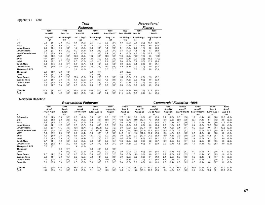
47

Appendix 1 – cont.Troll

FisheriesRecreational

Fishery1999 1999 1998 1999 1998 1999 1998 1998

Area125 Area126 Area127 Area127 Area 124-127 Area 124-127 Area 24 Area25

Aug1-13 Jul 26- Aug13 Jul31- Aug7 Jul26- Aug4 Aug 1-16 Jul 23-Aug2 July26-Aug1 July24-Sept25N 142 219 155 177 106 195 91 18QCI 0.8 (1.4) 0.0 (0.7) 0.1 (1.6) 3.6 (1.7) 0.3 (2.1) 1.3 (0.9) 3.1 (2.3) 10.7 (8.9)Nass 0.3 (1.2) 2.0 (1.2) 0.0 (0.8) 0.0 (1.1) 6.9 (3.9) 0.1 (0.9) 0.0 (0.2) 9.9 (8.0)Upper Skeena 2.0 (1.4) 0.0 (0.8) 1.2 (1.2) 0.0 (0.5) 1.4 (2.3) 1.1 (1.2) 2.3 (1.4) 0.0 (2.9)Lower Skeena 2.3 (2.1) 1.8 (2.2) 0.0 (1.1) 3.9 (2.6) 2.6 (3.4) 2.3 (1.9) 1.3 (1.8) 4.3 (8.0)North/Central Coast 5.2 (2.9) 4.3 (2.3) 4.8 (3.2) 12.3 (3.9) 8.4 (3.9) 4.1 (2.0) 4.8 (2.8) 19.9 (11.2)WCVI 16.5 (4.2) 18.9 (3.9) 15.0 (5.3) 19.2 (3.9) 28.3 (6.9) 19.9 (3.5) 74.0 (7.4) 9.3 (10.9)ECVI 16.4 (4.6) 11.7 (2.7) 11.9 (4.4) 12.0 (4.3) 8.6 (4.9) 10.1 (3.4) 0.0 (2.6) 18.6 (13.2)NCVI 2.4 (2.2) 7.7 (2.6) 8.0 (3.6) 14.7 (4.1) 7.1 (4.2) 7.8 (2.8) 5.9 (5.3) 13.1 (9.6)South Main 3.8 (2.8) 6.8 (3.1) 5.7 (3.7) 7.8 (4.2) 7.9 (5.5) 3.9 (2.5) 3.4 (3.6) 0.0 (4.1)Lower Fraser 29.7 (5.0) 28.9 (4.2) 16.0 (4.9) 12.9 (3.6) 15.4 (6.5) 26.8 (4.1) 0.0 (1.0) 0.0 (1.4)Thompson/UPFR 3.1 (1.6) 3.8 (2.1) 0.0 (1.0) 5.8 (5.3)Thompson 3.1 (1.9) 3.0 (1.5) 0.0 (0.4) 0.8 (0.9)UPFR 4.5 (2.1) 0.0 (0.6) 0.0 (0.6) 0.4 (0.5)Puget Sound 5.7 (3.0) 7.7 (2.6) 20.9 (5.6) 5.5 (2.9) 3.0 (3.7) 15.2 (3.6) 3.0 (2.5) 2.5 (6.2)Juan de Fuca 2.1 (1.7) 2.3 (1.6) 6.7 (3.5) 3.7 (2.3) 1.8 (2.6) 0.5 (1.3) 0.0 (0.0) 0.0 (2.8)Coastal Wash 3.6 (2.5) 4.6 (2.9) 6.1 (3.2) 2.2 (1.9) 4.5 (3.0) 3.1 (2.1) 2.1 (2.2) 0.0 (6.1)Columbia 1.6 (1.7) 0.3 (0.8) 0.5 (1.2) 2.3 (1.5) 0.0 (0.0) 2.6 (1.5) 0.0 (0.0) 5.9 (5.3)

{Canada 87.0 (4.1) 85.1 (3.8) 65.8 (5.8) 86.4 (4.2) 90.7 (5.5) 78.6 (4.3) 94.8 (3.2) 91.6 (9.4){U.S. 13.0 (4.1) 14.9 (3.8) 34.2 (5.8) 13.6 (4.2) 9.4 (5.5) 21.4 (4.3) 5.2 (3.2) 8.4 (9.4)

Northern BaselineRecreational Fisheries Commercial Fisheries -1998

1998 1999 1998 1999 1999 Seine Seine Troll Troll Gillnet Seine Seine SeineArea3 Area3 Area4 Area4 Langara Isl. Area 1 Area 2W Area2W Area2W Area2E Area2E Area 3 Area3

July 25-Aug23 Jul 26 July 25-Aug 15 Jul 25-Aug 15 Aug 23 Aug 8-22 Aug 22-29 Jul 25-Aug1 Aug 8-29 Sep 19-Oct 10 Sep 19-Oct 10 Jul 18-Aug 1 Aug 2- 8N 71 135 67 30 71 21 12 99 152 123 260 153 498S.E. Alaska 5.6 (4.3) 6.0 (3.5) 2.0 (2.6) 0.0 (3.9) 0.0 (2.7) 17.5 (10.5) 0.0 (3.0) 4.7 (3.0) 5.1 (2.7) 3.5 (2.6) 1.9 (1.4) 9.9 (4.0) 18.3 (2.8)QCI 7.2 (4.2) 3.0 (2.0) 9.0 (4.5) 5.2 (3.9) 29.8 (7.1) 12.8 (9.7) 20.9 (12.1) 7.3 (4.2) 12.6 (3.8) 68.9 (5.6) 69.1 (4.4) 0.7 (1.2) 2.0 (0.9)Nass 6.6 (4.5) 5.2 (3.7) 0.0 (2.7) 6.5 (4.2) 10.2 (5.7) 0.0 (1.8) 0.0 (4.1) 1.3 (1.4) 0.0 (1.4) 0.0 (0.6) 2.3 (1.6) 5.4 (3.0) 11.7 (2.3)Upper Skeena 10.2 (4.1) 12.9 (3.9) 7.5 (3.7) 6.6 (4.7) 0.0 (2.0) 0.0 (0.5) 0.0 (0.0) 3.0 (2.4) 0.0 (1.0) 0.0 (0.7) 0.4 (0.5) 15.0 (3.8) 3.8 (1.5)Lower Skeena 7.0 (5.3) 14.7 (4.9) 16.6 (5.7) 17.3 (10.3) 8.2 (5.2) 8.8 (7.6) 8.9 (10.3) 6.9 (3.3) 1.1 (1.8) 2.1 (1.4) 0.0 (0.9) 9.6 (4.4) 12.3 (2.8)North/Central Coast 35.7 (7.8) 29.2 (5.4) 43.4 (8.8) 28.2 (10.8) 19.4 (6.6) 9.5 (10.4) 38.9 (16.5) 10.1 (4.4) 23.5 (5.6) 3.3 (2.7) 7.5 (2.6) 20.8 (4.8) 29.0 (3.3)WCVI 3.0 (3.2) 4.9 (2.6) 8.1 (4.4) 0.0 (0.9) 1.7 (3.0) 24.3 (11.2) 21.0 (14.6) 13.4 (6.3) 13.3 (4.8) 6.2 (3.9) 5.6 (2.5) 5.2 (3.0) 3.0 (1.8)ECVI 1.5 (4.0) 9.3 (3.5) 0.1 (3.7) 12.7 (7.2) 0.0 (2.0) 0.0 (2.4) 0.0 (10.1) 24.2 (6.3) 11.9 (4.5) 2.3 (3.0) 2.8 (2.3) 11.1 (4.7) 2.3 (1.9)NCVI 6.1 (4.3) 5.6 (2.8) 3.7 (4.4) 11.7 (7.9) 7.5 (4.5) 10.2 (9.2) 0.0 (4.1) 5.5 (4.1) 7.5 (3.9) 7.8 (3.6) 3.4 (2.6) 6.2 (3.2) 9.0 (2.3)South Main 7.7 (4.1) 7.2 (3.0) 3.6 (4.6) 0.0 (5.5) 6.9 (4.4) 16.3 (9.2) 0.0 (6.3) 6.2 (3.7) 10.9 (3.5) 0.6 (1.1) 3.9 (2.0) 3.0 (2.5) 3.5 (2.3)Lower Fraser 1.8 (3.2) 1.7 (2.2) 0.1 (2.8) 0.0 (3.4) 5.4 (4.1) 0.0 (1.3) 0.0 (0.0) 0.1 (2.9) 2.9 (2.7) 4.8 (2.8) 1.7 (1.4) 6.2 (3.3) 0.0 (0.9)Thompson/UPFR 0.0 (0.1) 1.4 (1.3)Thompson 0.0 (0.1) 3.8 (4.3) 0.0 (0.0)UPFR 0.0 (0.0) 0.0 (2.2) 0.0 (0.0) 0.0 (0.2) 0.0 (0.0) 0.0 (0.0) 2.0 (1.6) 0.0 (0.4) 0.6 (0.7) 0.0 (0.2) 0.7 (0.6) 0.3 (0.4)Puget Sound 7.7 (4.2) 0.0 (1.6) 0.0 (0.6) 3.4 (4.0) 0.0 (1.3) 0.0 (5.8) 10.3 (9.1) 3.0 (3.2) 2.2 (2.0) 0.1 (2.3) 1.5 (1.1) 3.7 (3.3) 1.8 (1.2)Juan de Fuca 0.0 (1.4) 0.0 (0.7) 2.6 (2.6) 0.0 (1.5) 0.0 (2.6) 0.0 (2.5) 0.0 (3.5) 8.1 (4.0) 2.4 (2.8) 0.0 (0.3) 0.0 (0.1) 1.2 (1.7) 0.7 (0.9)Coastal Wash 0.0 (0.5) 0.4 (0.9) 2.1 (2.3) 4.1 (3.6) 10.9 (4.6) 0.7 (4.1) 0.0 (2.0) 4.2 (3.0) 6.7 (2.7) 0.0 (0.2) 0.0 (0.5) 1.3 (1.6) 2.1 (1.0)Columbia 0.0 (0.5) 0.0 (0.3) 0.0 (0.0) 0.6 (3.0) 0.0 (0.9) 0.0 (0.0) 0.0 (0.0) 0.0 (1.0) 0.0 (0.4) 0.0 (0.9) 0.0 (0.1) 0.0 (0.7) 0.2 (0.5)

{Canada 86.7 (5.6) 93.6 (3.9) 93.4 (5.0) 91.9 (6.4) 89.1 (5.3) 81.8 (11.4) 89.7 (10.1) 80.0 (5.3) 83.7 (4.0) 96.5 (3.3) 96.6 (1.9) 83.9 (5.1) 77.0 (3.3){U.S. 13.3 (5.6) 6.4 (3.9) 6.7 (5.0) 8.1 (6.4) 10.9 (5.3) 18.2 (11.4) 10.3 (10.1) 20.0 (5.3) 16.3 (4.0) 3.6 (3.3) 3.4 (1.9) 16.1 (5.1) 23.0 (3.3)

48

Appendix 1 – cont.Commercial Fisheries 1998

Seine Gillnet Gillnet Seine Seine Seine Seine Seine GillnetArea3 Area3 Area4 Area6 Area6 Area6 Area6 Area6 Area6

Aug 15-31 Jul 11- Aug 22 Jul18-25 July12-18 Jul19-25 Jul26-Aug1 Aug2-8 Aug16-22 Jul25-Aug29N 90 25 8 116 232 111 109 36 76

S.E. Alaska 6.8 (7.7) 21.8 (10.7) 8.4 (10.5) 11.0 (5.3) 3.9 (2.8) 0.9 (1.9) 5.9 (4.0) 3.4 (2.8) 2.1 (4.3)QCI 5.3 (3.4) 0.0 (2.2) 26.4 (17.0) 1.4 (3.3) 0.8 (1.6) 2.3 (2.5) 2.5 (2.1) 3.9 (3.4) 0.0 (0.9)Nass 0.0 (4.0) 0.0 (6.9) 0.0 (0.0) 0.0 (2.3) 0.0 (0.4) 0.0 (1.4) 4.6 (2.9) 0.0 (3.5) 5.4 (4.7)Upper Skeena 1.3 (2.7) 8.6 (5.9) 23.7 (14.6) 0.9 (2.6) 0.0 (0.7) 0.3 (1.0) 1.5 (1.5) 0.0 (0.5) 2.5 (1.5)Lower Skeena 3.2 (5.2) 22.7 (12.3) 0.0 (5.7) 19.7 (6.7) 9.5 (3.7) 1.4 (3.2) 4.7 (3.9) 17.3 (8.4) 0.0 (3.7)North/Central Coast 35.7 (9.7) 22.0 (10.4) 0.5 (11.2) 35.7 (8.7) 55.5 (6.0) 40.6 (8.8) 61.6 (6.4) 51.7 (12.5) 69.7 (10.4)WCVI 5.0 (4.2) 21.7 (8.9) 19.7 (16.8) 7.6 (5.2) 0.1 (1.5) 3.9 (4.8) 2.8 (3.2) 4.2 (5.2) 2.0 (2.4)ECVI 6.3 (4.6) 0.0 (2.1) 16.2 (17.0) 0.4 (4.2) 7.2 (3.4) 0.9 (4.7) 13.5 (4.5) 8.0 (6.8) 0.0 (2.6)NCVI 12.8 (7.7) 0.0 (0.7) 5.0 (10.1) 4.8 (3.7) 3.5 (2.6) 9.9 (5.3) 0.0 (1.4) 6.6 (7.5) 6.1 (4.0)South Main 5.4 (4.8) 0.0 (3.9) 0.0 (0.5) 11.5 (5.8) 9.1 (3.9) 19.1 (8.4) 0.1 (3.3) 0.0 (2.8) 7.1 (4.5)Lower Fraser 5.5 (4.5) 0.0 (3.8) 0.0 (3.5) 0.0 (2.7) 6.5 (3.1) 5.6 (4.4) 1.7 (2.6) 0.1 (3.5) 0.0 (0.8)Thompson/UPFR 0.0 (1.4) 3.3 (3.4) 0.0 (4.3) 0.0 (0.6) 0.4 (0.6) 0.9 (1.2) 0.0 (0.1) 2.6 (2.6) 0.0 (0.0)Puget Sound 1.2 (3.6) 0.0 (5.5) 0.0 (4.7) 3.6 (4.9) 2.5 (2.5) 4.7 (3.2) 0.0 (1.0) 0.0 (1.6) 1.5 (3.0)Juan de Fuca 0.0 (1.2) 0.0 (1.2) 0.0 (0.0) 2.1 (1.8) 0.0 (0.6) 1.1 (3.1) 1.2 (1.3) 2.3 (2.3) 2.7 (2.2)Coastal Wash 11.6 (6.0) 0.0 (3.8) 0.0 (9.0) 1.3 (2.8) 0.0 (1.5) 3.0 (4.1) 0.0 (1.5) 0.0 (2.1) 0.0 (3.4)Columbia 0.0 (0.4) 0.0 (0.0) 0.0 (0.0) 0.0 (0.8) 1.1 (0.8) 5.4 (3.4) 0.0 (0.2) 0.0 (0.7) 1.0 (3.0)

{Canada 80.5 (8.7) 78.2 (11.1) 91.6 (13.7) 82.0 (6.7) 92.5 (3.8) 84.9 (6.7) 93.0 (4.4) 94.4 (4.8) 92.7 (6.7){U.S. 19.5 (8.7) 21.8 (11.1) 8.4 (13.7) 18.0 (6.7) 7.5 (3.8) 15.1 (6.7) 7.0 (4.4) 5.6 (4.8) 7.3 (6.7)

Fraser BaselineLWFR River Fisheries (Area29) Selective Fisheries

1997 1997 1998 1999 1998 1998 1999 1999 1999 1999

Seine Gillnet Gillnet Gillnet Gillnet Gillnet

pink tag Cottonwood Whonnock Sel#371 SelKadi Sooktrap DarcieHookAug29-Oct1 Oct15-Nov4 Aug 1-25 Oct10-Nov6 Aug26-Sept17 Sept4-Sept21 Oct16-31 Oct16-30 Sep27-Oct22 Sep29-Oct24

N 209 18 22 82 49 22 34 23 28 160LWFR 33.9 (3.3) 93.6 (6.4) 85.6 (9.1) 94.7 (2.6) 25.5 (8.5) 19.0 (10.8) 97.0 (3.6) 95.8 (4.0) 95.0 (3.9) 97.2 (1.8)Thompson/UPFR 66.1 (3.3) 6.4 (6.4) 14.4 (9.1) 74.6 (8.5) 81.0 (10.8)Thompson 4.6 (2.4) 2.7 (2.8) 4.2 (3.7) 0.0 (2.3) 2.8 (1.6)UPFR 0.7 (1.5) 0.3 (2.8) 0.0 (2.5) 5.0 (3.7) 0.0 (0.9)

49

Appendix 2. Coho DNA mixed stock estimates for year 2000 sampling, N = number of fish in sample. Standard deviations are in brackets.

Southern Baseline SeineFisheries

RecreationalFisheries U.S Net Fisheries

PSC Seine Test

PSCGillnetTest

Area20 Area123 Area 20-1 Area 23 Area 23 Area7a&7(nontreat)

Area7(reef)

Area7(reef)

Area7(reef)

Area 7a(Treaty)

Jul19-22 Jul23-29 Jul30-Aug5 Aug6-12 Aug13-19 Jun20-Jul7 July13-Aug6

Aug20(JOT)

Sep25-Oct5

Aug12-19 Aug1-5 Aug2-Sep3 Aug 15-16 Sep10-23 24-Sep Oct 1-8 1-Sep

N 199 176 190 190 199 164 105 66 194 4 156 57 123 154 130 83 11WCVI 5.5 (2.6) 3.0 (2.2) 5.8 (2.5) 2.7 (2.0) 2.7 (2.1) 8.1 (3.3) 6.9 (4.0) 0.0 (2.5) 8.9 (3.1) 25.1 (22.7) 63.3 (4.6) 63.3 (7.2) 4.7 (3.1) 2.3 (2.2) 5.9 (3.2) 5.5 (3.2) 0.0 (4.6)ECVI 8.7 (3.3) 20.8 (4.5) 18.2 (4.0) 16.4 (3.7) 26.8 (4.9) 14.2 (4.8) 20.9 (7.0) 23.1 (7.2) 15.6 (4.0) 27.1 (26.8) 6.7 (2.7) 9.4 (5.0) 7.4 (3.2) 14.4 (4.9) 33.8 (5.7) 18.1 (6.7) 15.8 (12.4)NCVI 4.8 (2.5) 3.8 (2.5) 1.8 (1.8) 5.3 (2.4) 0.3 (2.0) 6.3 (3.5) 3.0 (2.4) 10.8 (5.8) 1.8 (1.7) 0.0 (0.0) 9.2 (3.7) 8.6 (5.5) 3.8 (2.7) 3.1 (2.3) 2.4 (1.9) 0.7 (2.1) 15.5 (11.8)S. Main 10.5 (3.7) 5.5 (2.9) 9.6 (3.4) 10.6 (3.9) 14.8 (3.3) 26.4 (5.4) 35.2 (6.2) 6.8 (6.2) 12.9 (4.3) 23.5 (20.5) 6.6 (4.0) 7.4 (4.9) 69.9 (5.3) 8.9 (3.4) 6.6 (3.8) 14.5 (5.2) 0.4 (7.9)L. Fraser 17.1 (4.0) 29.5 (4.4) 21.2 (4.1) 18.4 (4.4) 15.2 (3.3) 5.1 (3.6) 7.6 (4.4) 15.5 (6.3) 31.8 (4.9) 0.0 (10.0) 2.5 (1.7) 4.4 (3.4) 4.2 (2.4) 42.9 (5.4) 41.9 (5.7) 47.1 (6.6) 56.5 (18.9)Thompson 1.1 (0.8) 1.1 (0.7) 0.9 (0.8) 0.8 (0.9) 0.1 (0.4) 0.0 (0.3) 1.3 (1.2) 1.5 (1.7) 0.0 (0.9) 0.0 (0.0) 0.0 (0.0) 0.0 (0.0) 1.0 (1.2) 10.5 (3.3) 2.2 (1.5) 0.0 (0.0) 0.0 (4.7)UPFR 0.0 (0.0) 0.0 (0.0) 0.0 (0.2) 0.0 (0.5) 0.4 (0.5) 0.0 (0.3) 0.0 (0.7) 0.0 (0.0) 1.5 (1.1) 0.0 (0.0) 1.0 (0.8) 0.0 (1.0) 2.0 (1.4) 7.9 (2.9) 0.0 (0.6) 0.0 (0.0) 0.0 (0.5)Puget S. 30.3 (4.7) 23.7 (4.8) 24.7 (4.5) 27.2 (4.6) 32.3 (4.6) 21.3 (4.6) 13.4 (5.0) 31.7 (8.8) 15.7 (4.1) 24.2 (22.6) 6.2 (2.2) 4.6 (3.6) 6.3 (2.8) 6.8 (3.2) 7.2 (3.5) 12.8 (4.7) 0.0 (9.9)J. de Fuca 9.4 (3.1) 7.9 (2.9) 8.8 (3.0) 3.5 (1.8) 1.0 (1.4) 4.2 (2.4) 1.8 (2.0) 7.4 (4.0) 6.0 (2.1) 0.0 (0.0) 0.9 (1.3) 0.0 (1.4) 0.6 (1.1) 2.3 (2.6) 0.0 (0.8) 0.6 (2.3) 0.0 (0.5)C. Wash 7.7 (3.0) 2.9 (2.0) 2.9 (2.2) 5.8 (2.6) 3.2 (1.7) 6.4 (2.6) 4.2 (3.4) 1.5 (4.5) 4.2 (2.9) 0.0 (3.9) 0.6 (1.0) 0.0 (1.2) 0.2 (0.8) 1.1 (1.4) 0.0 (1.5) 0.7 (2.2) 11.8 (10.1)Columbia 4.9 (1.6) 1.9 (1.3) 6.1 (2.3) 9.2 (2.7) 3.2 (1.6) 8.1 (2.7) 5.7 (2.5) 1.8 (2.0) 1.7 (1.4) 0.0 (0.0) 3.1 (1.6) 2.4 (2.1) 0.0 (0.5) 0.0 (0.4) 0.0 (0.8) 0.0 (0.4) 0.0 (2.7)

{Canada 47.7 (5.6) 63.5 (4.7) 57.4 (5.1) 54.3 (4.8) 60.3 (4.4) 60.1 (5.9) 74.9 (6.5) 57.7 (8.7) 72.5 (4.9) 75.8 (22.4) 89.3 (2.8) 93.0 (4.5) 92.9 (3.4) 89.8 (3.9) 92.8 (3.8) 85.9 (5.3) 88.2 (13.6){US 52.3 (5.6) 36.5 (4.7) 42.6 (5.1) 45.7 (4.8) 39.7 (4.4) 40.0 (5.9) 25.1 (6.5) 42.3 (8.7) 27.5 (4.9) 24.2 (22.4) 10.7 (2.8) 7.0 (4.5) 7.2 (3.4) 10.2 (3.9) 7.2 (3.8) 14.1 (5.3) 11.8 (13.6)

Central BaselineTroll Fisheries Seine/Troll FSC Seine

Area 11 Area12 Area12 Area125 Area126 Area 13 Area12 Area 12 Area 12 Area 12 Area 13 Area 13 Area 12/13 Area 12/13 Area 12/13 Area 25Aug2-3 Aug 2-5 Aug6-12 Jul29-Aug1 Jul30-

Oct11Aug8-21 Aug 25 Aug6-10 Aug14-17 Aug23-

Oct4Aug9-23 Oct2-8 Oct4-5 Oct12 Oct19-

Nov6Oct11-12

N 5 109 89 40 93 35 7 83 175 64 49 88 55 91 51 5QCI 0.0 (1.8) 0.8 (1.3) 0.5 (1.8) 0.0 (0.3) 3.0 (2.2) 0.0 (0.0) 0.0 (0.0) 0.4 (1.1) 0.4 (1.1) 11.1 (4.7) 1.0 (2.0) 0.8 (1.9) 0.0 (1.0) 0.3 (2.4) 0.0 (2.0) 0.0 (0.1)Nass 0.0 (0.0) 0.0 (0.8) 4.1 (2.6) 0.0 (1.3) 0.0 (1.2) 2.0 (3.1) 0.0 (0.0) 1.7 (3.1) 0.5 (1.3) 5.3 (4.3) 0.0 (0.6) 0.0 (1.5) 1.3 (2.1) 2.6 (3.5) 0.0 (1.3) 20.2 (18.7)Upper Skeena 0.0 (0.0) 0.8 (1.0) 0.0 (0.4) 0.0 (1.5) 1.0 (1.0) 5.3 (3.4) 0.0 (0.0) 0.0 (1.6) 0.0 (0.6) 1.4 (2.6) 2.2 (1.9) 2.6 (2.2) 1.7 (2.2) 0.4 (1.8) 2.9 (2.6) 0.0 (0.0)Lower Skeena 0.0 (6.0) 0.7 (2.5) 1.5 (3.1) 0.5 (4.7) 0.0 (2.6) 0.0 (4.8) 0.0 (0.0) 7.0 (4.5) 2.1 (2.3) 0.0 (1.8) 8.1 (4.7) 0.0 (1.8) 1.4 (4.2) 2.9 (3.5) 2.4 (2.9) 0.0 (9.0)North/Central Coast 60.6 (27.3) 26.0 (5.7) 20.5 (6.9) 7.8 (6.0) 8.9 (3.3) 10.8 (9.8) 36.2 (20.7) 14.5 (8.3) 40.2 (5.6) 11.6 (6.3) 8.9 (6.7) 2.6 (5.5) 9.6 (7.1) 14.7 (5.6) 2.7 (5.0) 16.7 (22.2)

WCVI 0.0 (16.2) 3.2 (3.2) 16.8 (5.5) 14.0 (6.9) 6.9 (3.8) 2.5 (4.0) 0.0 (5.9) 8.5 (3.9) 9.8 (4.2) 2.1 (4.0) 1.1 (4.0) 7.7 (3.3) 7.1 (4.3) 0.0 (2.1) 3.1 (4.1) 24.8 (16.3)

ECVI 1.3 (14.1) 27.7 (5.4) 20.5 (6.7) 1.8 (5.9) 16.2 (5.3) 24.6 (8.4) 17.1 (15.5) 24.3 (6.4) 1.3 (2.5) 45.7 (8.3) 15.2 (6.6) 29.8 (6.0) 29.2 (9.0) 21.4 (7.7) 21.8 (9.4) 0.1 (11.8)NCVI 18.6 (15.6) 18.0 (5.8) 13.7 (4.9) 10.4 (6.4) 12.0 (5.1) 1.5 (2.8) 0.0 (3.0) 1.5 (2.9) 7.3 (3.4) 3.3 (3.5) 4.2 (3.5) 0.3 (3.6) 2.8 (3.5) 6.3 (3.9) 8.8 (6.3) 38.1 (25.4)South Main 0.0 (2.1) 10.3 (4.5) 13.7 (5.5) 12.7 (6.1) 4.9 (2.8) 43.1 (12.0) 31.7 (21.4) 28.3 (6.9) 20.9 (4.9) 3.0 (3.8) 25.5 (9.5) 16.8 (5.7) 15.5 (7.9) 8.2 (5.7) 10.4 (6.7) 0.0 (8.3)Lower Fraser 0.0 (0.0) 4.0 (3.5) 6.1 (3.8) 1.4 (3.5) 19.1 (5.5) 4.1 (7.5) 0.0 (12.7) 5.4 (3.2) 12.1 (3.8) 9.1 (4.3) 30.1 (9.7) 21.1 (5.5) 14.1 (5.9) 27.5 (6.8) 23.1 (8.0) 0.0 (0.0)Thompson 0.0 (0.0) 0.0 (0.0) 0.0 (0.0) 1.9 (3.2) 1.8 (1.5) 0.0 (1.1) 0.0 (0.0) 0.5 (2.0) 0.6 (0.6) 0.0 (0.5) 0.0 (0.4) 0.4 (1.3) 2.3 (2.2) 0.0 (1.7) 0.0 (2.2) 0.0 (7.3)UPFR 0.0 (0.1) 1.6 (1.6) 0.0 (0.0) 3.1 (3.2) 1.3 (1.3) 0.0 (0.0) 0.0 (0.0) 0.7 (1.8) 0.3 (0.8) 1.5 (2.1) 0.0 (0.0) 0.0 (0.5) 0.0 (0.6) 0.0 (0.0) 1.2 (1.9) 0.0 (0.0)Puget Sound 0.0 (0.0) 1.8 (1.6) 0.0 (2.0) 35.0 (8.2) 10.9 (5.1) 6.1 (5.9) 2.0 (13.0) 0.6 (2.2) 2.9 (2.1) 5.9 (4.3) 0.0 (1.1) 10.5 (4.3) 7.6 (4.3) 5.4 (4.5) 9.4 (5.5) 0.0 (2.9)Juan de Fuca 0.0 (0.0) 1.8 (1.7) 0.0 (1.2) 6.9 (5.3) 3.2 (2.6) 0.0 (0.0) 13.0 (10.8) 0.0 (0.6) 1.2 (1.5) 0.0 (0.4) 3.0 (2.6) 0.0 (2.0) 5.6 (3.4) 7.9 (5.0) 5.5 (6.7) 0.0 (7.5)Coastal Wash 19.4 (20.4) 3.2 (1.8) 2.7 (1.9) 4.6 (4.5) 10.7 (4.3) 0.0 (1.0) 0.0 (7.3) 1.4 (1.9) 0.0 (1.1) 0.0 (0.0) 0.74 (1.7) 6.4 (3.7) 1.9 (3.1) 0.7 (1.8) 2.1 (4.1) 0.0 (0.0)Columbia 0.0 (0.0) 0.0 (1.2) 0.0 (0.0) 0.0 (0.2) 0.0 (1.5) 0.0 (0.0) 0.0 (0.0) 5.4 (2.7) 0.5 (0.8) 0.0 (0.0) 0 (1.0) 1.0 (1.4) 0.0 (1.0) 1.7 (2.2) 6.5 (5.0) 0.0 (0.0)

{Canada 80.6 (20.5) 93.2 (3.0) 97.3 (2.8) 53.6 (9.4) 75.2 (6.0) 94.0 (6.0) 85.0 (15.1) 92.7 (4.4) 95.4 (2.8) 94.1 (4.3) 96.29 (3.4) 82.1 (5.9) 84.8 (6.3) 84.3 (7.2) 76.4 (9.1) 100.0 (7.9){U.S. 19.4 (20.5) 6.8 (3.0) 2.7 (2.8) 46.5 (9.4) 24.8 (6.0) 6.1 (6.0) 15.0 (15.1) 7.3 (4.4) 4.6 (2.8) 5.9 (4.3) 3.71 (3.4) 17.9 (5.9) 15.2 (6.3) 15.7 (7.2) 23.6 (9.1) 0.0 (7.9)

50

Appendix 2 –cont.GillnetFishery

RecreationalFisheries

Area12 Area13 Area12,13 Area 24Aug2-27 Aug2-Oct9 Aug11 Aug13-26

N 30 9 3 14QCI 1.9 (3.1) 11.8 (11.7) 16.8 (26.4) 0.0 (2.1)Nass 0.0 (3.6) 0.0 (7.6) 0.0 (0.0) 0.0 (0.0)Upper Skeena 0.0 (2.8) 0.0 (3.5) 0.0 (0.0) 0.0 (0.7)Lower Skeena 7.6 (6.4) 0.0 (4.6) 0.0 (0.0) 3.9 (7.0)North/Central Coast 28.2 (10.7) 11.6 (14.0) 0.0 (6.5) 18.7 (12.5)WCVI 14.2 (6.6) 0.0 (9.3) 80.9 (33.9) 36.3 (16.6)ECVI 12.3 (7.7) 33.3 (20.2) 0.0 (0.0) 7.5 (9.9)NCVI 3.7 (4.5) 0.0 (3.6) 0.0 (1.0) 22.0 (15.9)South Main 29.4 (9.9) 20.3 (12.1) 0.1 (6.6) 11.6 (10.9)Lower Fraser 0.0 (3.4) 11.6 (14.4) 0.0 (1.4) 0.0 (2.0)Thompson 0.0 (0.0) 0.0 (0.0) 2.1 (16.2) 0.0 (0.0)UPFR 0.0 (1.5) 0.0 (0.0) 0.0 (0.0) 0.0 (0.0)Puget Sound 2.7 (4.6) 0.0 (2.7) 0.0 (0.0) 0.0 (0.0)Juan de Fuca 0.0 (1.0) 0.0 (5.9) 0.0 (0.0) 0.0 (1.4)Coastal Wash 0.0 (1.9) 11.4 (13.7) 0.0 (0.0) 0.0 (0.0)Columbia 0.0 (2.1) 0.0 (0.0) 0.0 (0.0) 0.0 (0.0)

{Canada 97.4 (5.2) 88.6 (15.0) 99.98 0.02 100.0 (1.4){U.S. 2.7 (5.2) 11.4 (15.0) 0.02 0.02 0.0 (1.4)

51

Appendix 3. Estimated fishery exploitation rates (expl), adjusted historical escapements (esc), marine fishery catches and total abundances (abund) forinterior Fraser River watershed coho salmon.

Return South Thompson North Thompson Lower Thompson Non-Thompson Fraser

Year expl esc catch abund esc catch abund esc catch abund esc catch abund

1975 0.68 5864 12490 18354 22286 47468 697541976 0.68 3920 8349 12268 20675 44037 647131977 0.68 8490 18082 26572 42804 91171 1339751978 0.68 7996 17032 25028 39095 83269 1223641979 0.68 10198 21720 31918 47819 101851 1496701980 0.68 7025 14964 21989 10542 22454 329961981 0.68 4120 8775 12895 20615 43909 645241982 0.68 5849 12459 18308 42295 90087 1323821983 0.68 6196 13196 19392 35086 74731 1098161984 0.68 15394 32789 48183 69552 148141 217692 5155 12050 172051985 0.68 16998 36205 53204 45160 96188 141349 1913 4060 59731986 0.66 16521 31665 48186 104267 199846 304113 2211 4300 65111987 0.54 21087 24478 45564 54884 63710 118594 4208 4945 91531988 0.71 24426 60376 84802 70612 174539 245150 4013 9830 138431989 0.65 17208 31288 48496 30677 55779 86455 3423 6340 97631990 0.74 8609 24069 32677 25697 71844 97542 4421 12600 170211991 0.68 4160 8737 12896 14585 30633 45217 3794 8825 126191992 0.81 11886 52239 64125 22042 96875 118917 4905 21000 259051993 0.88 1873 13172 15045 9669 67999 77667 8416 61500 699161994 0.43 4485 3430 7915 10031 7671 17702 5252 3965 92171995 0.56 3622 4639 8261 22477 28794 51272 1984 2525 45091996 0.83 1760 8906 10667 12319 62325 74645 1209 5900 71091997 0.40 2034 1384 3418 6722 4573 11295 4217 2820 70371998 0.07 4946 375 5321 9125 685 9810 2628 200 2828 8147 610 87571999 0.09 3074 305 3379 8916 885 9801 5007 495 5502 5389 535 59242000 0.034 3785 134 3919 7032 250 7282 4459 157 4616 4723 144 4867

52

Appendix 4. Chen, D. G., J. R. Irvine, and A. Cass. Incorporating Allee effects in salmon stock-recruitment models and applications for determining reference points. Draft manuscript (in review).

AbstractA new type of stock-recruitment model is examined that incorporates Allee effects that may occur

when fish populations are small. The model is a natural extension of traditional stock-recruitmentmodels, which only consider density dependent effects when population densities are high. Since the newmodel is intrinsically nonlinear to the parameters, the theory of maximum likelihood estimation is used toestimate model parameters and the associated statistical inferences. Having found the local optima for thelikelihood function, a global genetic search algorithm is entertained to obtain the parameter estimates.Based on this extended model, an extinction probability curve is developed based on the parameterdefining the Allee effects in the new model. This curve can readily be used to calculate the theoreticalprobability of extinction for any particular spawner number or biomass. Alternatively, since managersmay wish to assign reference points corresponding to particular extinction probabilities, correspondingspawner numbers can be determined for these reference points. Data from North Thompson coho andChilko sockeye salmon are used to demonstrate the approach.

IntroductionThe analysis of fish stock-recruitment (S-R) is often the first step to evaluate and implement

fishery policies designed to optimize spawner numbers and exploitation rates. The analysis typicallybegins with the assumption of a functional relationship, denoted by F(•), between spawners and recruits:

(1) R S F St t t( , )

where St is the spawners at year t, t = 1 to n and Rt is the corresponding recruits for the spawners at thatbrood year t calculated as total escapements and catches. θ is a vector of parameters associated with thisrelationship and may be associated with a fishery management policy.

The two most commonly used functional forms based on biologically sound grounds are theBeverton-Holt model (Beverton-Holt 1957) and the Ricker model (Ricker 1975):

(2)t

tt S

SR

βα+

=1

Beverton-Holt Model

(3) tStt eSR βα −= Ricker Model

where α and β are the parameters to describe productivity of the population at low density, and capacitylimited by density dependence, respectively. As a unified S-R model, Deriso (1980) introduced anadditional shape parameter γ and proposed the following model:

(4) R S St t t( ) /1 1 Deriso Model

5 Manuscript submitted to Can. J. Fish. Aquat. Sci.

53

where γ is a shape parameter to modify the S-R relationship. It can be seen that the Beverton-Holt model(2) and Ricker model (3) are in fact special cases of the Deriso Model (4) when γ = -1 and γ → 0,respectively.

These models allow for compensatory mortality. At high population densities, resources willbecome limiting and recruits per spawner will decrease. However, the models ignore depensatorymortality, which may occur when the population is below some critical level. This is known as the Alleeeffect (Allee et al. 1949) when population growth declines as population density declines. A variety ofprocesses can result in depensation occurring at low population sizes. For example, inbreeding may occurand result in reduced survivals, spawning fish may not easily find mates, depensatory predation mayresult in higher proportions of fish being killed, poor conditioning of the spawning environment and lowefficiency of food location may all contribute to depensatory mortality at low spawner densities (Hilbornand Walters 1992; Emlen 1984; Asmussen 1979). When abundances are low, depensation (if it exists)will accelerate population declines and increase their probability of extinction (McElhany et al 2000).

Whether depensation is a significant factor for fish populations is not clear. Myers et al. (1995)found that 3 of 26 fish stocks had lower than expected recruits per spawner at low densities than would beexpected using a Beverton-Holt model. Liermann and Hilborn (1997) examined the same data and foundthat the most likely values for the stock recruit relationship were usually close to or within the range of nodepensation. However, since there was a significant amount of uncertainty about whether depensationexisted, Liermann and Hilborn concluded that analyses of stock recruitment data should incorporatespawner recruit curves that allow for the possibility of depensation.

Several approaches have been used to incorporate possible depensatory effects in the analysis ofstock recruit data. Hilborn and Walters (1992) recommended replacing αS with αSm where the powerparameter m is greater than 1.0. Liermann and Hilborn (1997) used a Bayesian hierarchical model toestimate the distribution describing the variability of depensation within various taxa. Routledge andIrvine (1999) introduced a cuttoff value c to allow for the effects of possible depensation at lowabundance and modified their formulas when S ≤ c. In the discussion of compensatory populationdynamics within a stock complex, Frank and Brickman (2000) were the first to introduce a S-R modelthat incorporated Allee effects by permitting a non-zero intercept representing recruitment failure.Incorporating depensation, the S-R model in equation (1) becomes:

(5) R S S F S St t offset t offsetd i d i,

where Soffset is the parameter associated with the Allee effects and is the offset from the origin representingzero recruitment (Frank and Brickman 2000). Hereafter model (5) will be called Allee S-R model. Forthe S-R models (2)–(4), the corresponding Allee S-R models would be:

(6))S(1

)S(

offset

offset

−+−

=t

tt S

SR

βα

(7) )S(offset

offset)S( −−−= tStt eSR βα

(8) R S St t t( )[ ( )] /S Soffset offset1 1

In this paper, we apply the maximum likelihood estimation (MLE) approach combined with aglobal search algorithm to estimate S-R parameters. We discuss the properties of the parameter Soffset

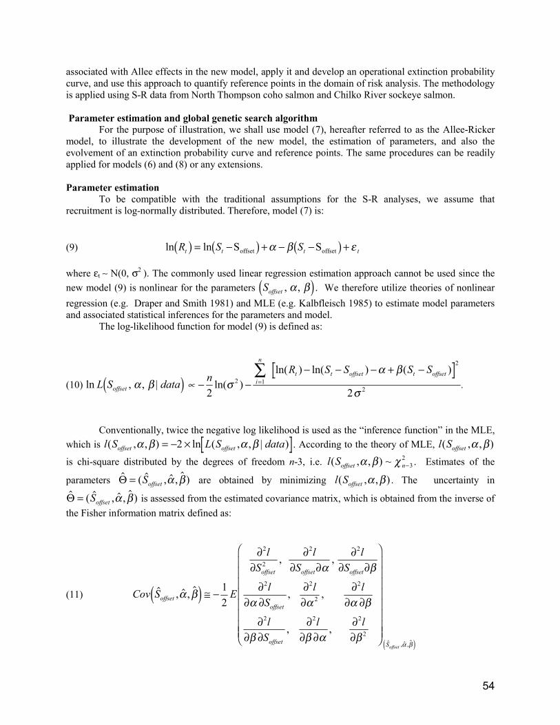
54

associated with Allee effects in the new model, apply it and develop an operational extinction probabilitycurve, and use this approach to quantify reference points in the domain of risk analysis. The methodologyis applied using S-R data from North Thompson coho salmon and Chilko River sockeye salmon.

Parameter estimation and global genetic search algorithmFor the purpose of illustration, we shall use model (7), hereafter referred to as the Allee-Ricker

model, to illustrate the development of the new model, the estimation of parameters, and also theevolvement of an extinction probability curve and reference points. The same procedures can be readilyapplied for models (6) and (8) or any extensions.

Parameter estimationTo be compatible with the traditional assumptions for the S-R analyses, we assume that

recruitment is log-normally distributed. Therefore, model (7) is:

(9) ln lnR S St t t tb g b g b gS Soffset offset

where εt ∼ N(0, σ2 ). The commonly used linear regression estimation approach cannot be used since thenew model (9) is nonlinear for the parameters Soffset , ,d i . We therefore utilize theories of nonlinearregression (e.g. Draper and Smith 1981) and MLE (e.g. Kalbfleisch 1985) to estimate model parametersand associated statistical inferences for the parameters and model.

The log-likelihood function for model (9) is defined as:

(10) ln , , |L S dataoffsetd i ∝ n

R S S S Si

n

t t offset t offset

2 22 1

2

2ln( )ln( ) ln( ) ( )

.

Conventionally, twice the negative log likelihood is used as the “inference function” in the MLE,which is l S L S dataoffset offset( , , ) ln ( , , | )2 . According to the theory of MLE, l Soffset( , , )is chi-square distributed by the degrees of freedom n-3, i.e. l Soffset n( , , ) ~ 3

2 . Estimates of the

parameters ( , , )Soffset are obtained by minimizing l Soffset( , , ) . The uncertainty in

( , , )Soffset is assessed from the estimated covariance matrix, which is obtained from the inverse ofthe Fisher information matrix defined as:

(11) Cov S E

lS

lS

lS

lS

l l

lS

l l

offset

offset offset offset

offset

offset Soffset

, ,

, ,

, ,

, ,, ,

e j

e j

F

H

GGGGGGGG

I

K

JJJJJJJJ

12

2

2

2 2

2 2

2

2

2 2 2

2

55

The estimated standard error for each parameter can be obtained from the corresponding elementsfrom (11). According to theory of MLE, the parameter estimates ,a b Soffsetand in (9) and (10) arenormally distributed as:

(12) ~ , ; ~ , ~ ,a N a b N b S N Sa b offset offset Soffset

2 2 2c h c h e jand .

Special attention is paid to the parameter Soffset since this parameter represents the number ofspawners that will theoretically produce zero recruitment (i.e. a high probability that this year class wouldgo extinct). We wish to evaluate whether including the Allee parameter Soffset improves the model fitfrom model (7) relative to the traditional Ricker model (3). Since models (3) and (7) are nested, thelikelihood ratio test can be used to test whether the inclusion of Soffset significantly improves the modelfit:

(13) l l Soffset( , ) ( , , ) ~ 12

where l( , ) and l Soffset( , , ) are twice the negative log likelihood function from models (3) and (7),respectively.

Global genetic search algorithmThe parameter estimates can be obtained from equation (10) by any search algorithms, including

gradient and hill-climbing search methods. These algorithms are known as local search algorithms wherethe initial starting points are essential. We found that there are local optima for the minimization ofequation (10) with only three parameters which led us to employ the global genetic search algorithm(GA). GA is a search algorithm from the mechanics of natural selection and genetics with naturalpopulations evolve according to the principles of “survival of the fittest”. (Holland 1975). The highly fitindividuals are given high opportunities to “reproduce”, by “cross breeding” with others in the population.GA differs from conventional search techniques, because it considers many points in the search spacesimultaneously, and therefore has a reduced chance of converging to some local optima. Since Holland(1975) introduced and investigated this algorithm, the approach has been used in many areas, such as incurve fitting, mathematical optimization, and training neural network models. Recent descriptions of theapproach with applications to fisheries are found in Saila (1996) and Chen et al. (2000).

To use the GA in this paper, we specify a large but reasonable range for each parameter in( , , )Soffset and randomly generate an initial population with 100 starting points. Based on the

fundamental “genetic” operators as reproduction, crossover and mutation, 10% of the best solutionsamong the 100 are reproduced. By analogy with a biological genetic system where mutations are rare, ahigher probability (80%) is given to the crossover process than to the mutation process (5%). Thisprovides a “crossover” mechanism for the search to mix and match desirable qualities through a randomprocess with the occasional “mutation” of a value at a particular search position.

56

Definition of an extinction probability curveSpawner numbers or biomass is the most readily available and also the most commonly used

quantity in fisheries research and management. Clearly we would like to manage fisheries above theparameter, Soffset , with known probability. Then the stock extinction probability function of the stock isdefined as Pr( ) Pr( )Stock Extinction S Soffset . Since Soffset can be estimated from the MLE (10) withthe distribution in (11), the operational definition of the extinction probability (denoted by OPr( )EP ) is:

(14) OP EPr S S S SS S

offset offsetoffset

Soffset

( ) Pr PrFHG

IKJd i d i 1

for any level of spawning biomass, S. In equation (14), ( ) is the cumulative density function for thenormal distribution. Since Soffset

in equation (14) is generally unknown, then the MLE estimate fromequation (11) can be used to give an estimate of OPr( )EP :

(15) OP EPr S S TS S

offsetoffset

Soffset

( ) PrFHG

IKJd i 1

where T( ) is the cumulative density function for the t-distribution with degrees of freedom n-3.Equation (15) can be used for two purposes. One is to calculate the probability of extinction for

any given spawner number or biomass S. Another is to obtain reference points for a given extinctionprobability that is based on an acceptable level of extinction risk.

Data ApplicationsNorth Thompson Coho

Identification of reference points and extinction probabilities at low spawner numbers are neededfor coho salmon from the Thompson River watershed in central British Columbia. Numbers of cohosalmon returning to the Thompson River have declined significantly in recent years and these fish havebeen the focus of much attention (Bradford and Irvine 2000). Precise estimates of spawner numbers areavailable for North Thompson coho commencing in 1975, and annual recruitment (catch plus spawningescapement) was estimated using a time series of fishery exploitation rates (Irvine et al. 2000):

(16) Rt = St /(1-explt)

where spawners were assumed to be all three years old and explt are the fishery exploitations at year t.We first fit the Ricker model (3) to S-R data for North Thompson coho by a simple regression approach,and then fit the same S-R data with the Allee Ricker S-R model (9) by the MLE with the GA approach(Fig. 1). Figure 2 illustrates the GA search algorithm with 100 points in the search space. It can be seenfrom Figure 2 that convergence is achieved after ~60 generations (a term used in GA, which is equivalentto “iterations” in any other search algorithms). Parameter estimates and the resulting value for the twice-negative likelihood function are summarized in Table 1. The Allee-Ricker model (9) gave the lowestvalue for the negative log-likelihood function indicating that the Allee-Ricker model fit the data best. This

57

conclusion can also be found from the likelihood ratio test in (13) since l l Soffset( , ) ( , , ) = 1.7.Although not significant at the 95% level, this is significant at the 80% confidence level ( 0 80 1

2. , =1.642),

which indicates that the inclusion of the parameter Soffset significantly improved the model fit. Weconclude that the Allee-Ricker model (9) should be used to analyze the S-R relationship. For the newmodel, the estimate of Soffset is 5,211 (Fig. 1) with a standard error of 1,680. Following the distribution in

(12) for Soffset , a distribution plot is given in Figure 3 with the 80% confidence interval. The 80%confidence interval is (2994, 7428); Soffset is statistically different from zero. Therefore the inclusion ofSoffset significantly improves the model fit, which is consistent with the result from the likelihood ratiotest.

With the new Allee-Ricker model (9), the operational extinction probability function from (15)can be constructed. Figure 4 illustrates the extinction probability as the function of spawner numbers.With this function, the extinction probability can be readily calculated for any given spawner number(Figure 4 and Table 2). Also, with any extinction probability suggested by managers, the correspondingspawner numbers can be calculated from this function as a management reference point (Figure 4). Table2 lists several reference points for particular probabilities.

Patterns in the residuals were examined after the Ricker model (3) was fit to the data. Noapparent relationship was seen between the size of the population and the residuals but there was evidenceof non-stationarity. A sequence of strong positive residuals in the early 1980’s preceded a declining trendwith negative residuals occurring in most recent years. In this instance, trends in the residuals do notnegate the value of calculating Soffset since recent low productivities (α) result in a positive bias inestimates of Soffset. We consider that a small positive bias when computing a reference point is acceptablesince it is risk averse. The patterns in the residuals may provide an explanation why the Allee-Rickermodel fit the data better than the traditional Ricker S-R model (Table 1). The first-order autocorrelationwas significant when the Ricker S-R model was applied (Lag 1, autocorrelation coefficient =0.42), butwas not when the Allee-Ricker model was fit to the data (Fig. 5).

Chilko SockeyeSpawner and recruit data for Chilko Lake sockeye are available for brood years 1948 to 1995

(Fig. 6). Chilko Lake is one of the largest producers of sockeye within the Fraser River watershed with anaverage of 340,000 spawners and 1.4 million recruits per year. This stock has rebuilt since the 1980s andthe numbers of spawners increased to nearly 700,000 per year since 1989. The S-R relationship suggeststhe stock is now near the maximum capacity of Chilko Lake. Chilko Lake was fertilized intermittently infour years beginning in 1987 and ending in 1992. Bradford et al. (2000) present evidence for increasedsockeye freshwater productivity as a result of fertilization. The S-R data used in our analysis excludes thefour years of fertilization to avoid potential problems of parameter bias.

We first fit the Ricker model (3) by a simple regression approach and then fit the Allee Ricker S-R model (9) by the MLE with the GA for the same data. The parameter estimates and the resulted valuefor the twice-negative likelihood function are summarized in Table 1. It can be seen that all the estimatesfor α and β are statistically significant along with the significant model fit. The estimate of Soffset is 1,585with standard error of 11,065. Figure 6 gives the S-R data series and the model fits. Because of the datarange and the small value of the estimated Soffset (=1,585), it is not obvious from Figure 6 to see thebehavior of Soffset . In order to see the end behavior of Soffset , a small range of data is plotted in Figure 7.

Following the distribution in (12) for Soffset , a distribution plot is given in Figure 8. It can be seenfrom this plot that 95% confidence interval covers 0, which means that Soffset is not statisticallysignificantly different from zero. Therefore the inclusion of Soffset does not significantly improve the

58

model fit. This conclusion can also be found from the likelihood ratio test in (13) sincel l Soffset( , ) ( , , )= 0.025 < 3.84 = 0 95 1

2. , .

Following the distribution in (12) for Soffset , a distribution plot is given in Figure 9 with the 95%confidence interval. The 95% confidence interval covers zero, which means that Soffset is not statisticallysignificantly different from zero. Therefore the inclusion of Soffset is not significantly improve the modelfit, which is consistent with the result from the likelihood ratio test.

In Figure 9 we illustrate the extinction probability for Chilko sockeye as the function of spawnernumbers. The extinction probability can be calculated for a given spawner abundance (Figure 9) anddepending on the level of risk tolerance, a management reference in terms of spawner abundance can becalculated from this function. Table 2 lists several reference points for the given probabilities.

DiscussionIn this paper we make several contributions to the field of conservation biology and in particular

the evaluation of extinction risk. Firstly, we demonstrate how traditional S-R models can be extended byincorporating potential Allee effects that may occur at low spawner densities. Methods to estimateparameters and associated statistical inferences are developed including the use of GA. Secondly, withthe extended Allee-SR model, we develop an operational formula for the extinction probability function.This formula can be used to calculate the extinction probability for any given spawner abundance, andalso allows managers the opportunity to define reference points according to particular extinctionprobabilities.

The precautionary approach is increasingly being applied in fisheries management to complywith international agreements for sustainable resource use (e.g. Richards and Maguire 1999). Thisapproach is intended to ensure that conservation takes precedence over other objectives (NMFS 1999).Reference points provide the primary mechanism by which the precautionary approach can be applied(Richards and Maguire 1999). In our paper we define the probability distribution associated with Soffset

and propose this as a suitable reference point that can be used by managers to minimize the possibility ofpopulation extinction.

Managers applying the precautionary approach would like a low probability of populations goingextinct. One way to do this is to “buffer” reference points by incorporating uncertainty. Sources ofuncertainty and statistical pitfalls that can bias stock-recruitment model parameters are discussed inHilborn and Walters (1992). These include lack of contrast in the spawning escapement variable,measurement errors in escapement and recruitment, temporal auto-correlation in the S-R series and non-stationarity of S-R relationships. Apart from the lack of contrast in the escapement time series, variousstatistical remedies can deal with S-R biases. To minimize the likelihood of a population falling belowthe Soffset, the limit should be set higher than the point estimate. For instance, one might wish to select areference point corresponding to the 10% extinction probability rather than the 50% value. Uncertainty inSoffset as a result of S-R bias should be carefully examined on a case specific basis as with any of theclassical S-R models. If there is a temporal pattern in productivity, one could model productivity as afunction of time. Reference points may need to be raised during periods of low productivity. Soffset couldbe used in a Bayesian decision analysis to evaluate the consequence of alternative management objectiveson extinction risk.

The two salmonid examples considered here demonstrate the potential effect of data variabilityuncertainty at low spawner densities on estimates of Soffset. For North Thompson coho, Soffset is statisticallysignificant from zero despite the variability in the data at low spawner densities. Because Soffset for Chilkosockeye is not significant, it is unclear if depensatory mortality at low spawner density is negligible or ifdepensatory mortality is masked by high survival variability and/or data measurement error. Liermannand Hilborn (1997) similarly concluded from their analysis of Chilko sockeye data that depensatorymortality at low spawner density is insignificant.

59

The extended model (5) can also be used to incorporate environmental information and fisheryinterventions, such as, R S S F S S Xt t offset t offset td i d i, , , where Xt is a vector of environmental andfishery intervention variables. This model can be combined with the semiparametric approach discussedin Chen and Irvine (2001) to analyse the compensatory and depensatory effects embedded in the S-Rrelationship with environmental and fishery interventions.

We feel that the new Allee S-R model is a useful extension for the traditional S-R model to beused for fishery S-R analysis, and we believe that the operational definition of the extinction probabilityfunction developed in this paper is a useful tool for fishery management.

AcknowledgementsWe thank Bill Clark, Steven Hare, Gayle Brown and Alan Sinclair for helpful comments on the

manuscript and approach.

ReferencesAllee, W.C., Emerson, A.E., Park,O., Park, T. and Schmidt, K.P. 1949. Principles of Animal

Ecology, Saunders, Philadephia.Asmussen, M.A. 1979. Density-dependent selection. II. The Allee effect. Am. Nat. 114: 796-809.Beverton, R. J. H. and Holt, S. J. 1957. On the dynamics of exploited fish population. Fish. Invest.

Ser. II. Mar. Fish. G.B. Minist. Agric. Fish. Food. Vol. 19.Bradford, M. J., and J. R. Irvine. 2000. Land use, fishing, climate change and the decline of Thompson

River, British Columbia, coho salmon. Can. J. Fish. Aquat. Sci. 57:13-16.Bradford, M. J., B. J. Pyper, and K. S. Shortreed, 2000. Biological responses of Sockeye Salmon to the

fertilization of Chilko Lake, a large lake in the interior of British Columbia. North Amer. J. Fish.Mgmt. 20 (3): 661–671.

Chen, D.G., N. B. Hargreaves, D. M. Ware and Y. Liu 2000. A fuzzy logic model with geneticalgorithm for analyzing fish stock-recruitment relationships. Can. J. Fish. Aquat. Sci. 57:1878-1887.

Chen, D.G. and J. R. Irvine. 2001. A semiparametric model to examine stock-recruitmentrelationships incorporating environmental data. Can. J. Fish. Aquat. Sci. 58: 1178-1186.

Draper, N.R. and H. Smith. 1981. Applied Regression Analysis. 2nd Edition. John Wiley & Sons.Inc.

Deriso, R.B. 1980. Harvesting strategies and parameter estimation for an age-structured model.Can. J. Fish. Aquat. Sci. 37: 268-282.

Emlen, J.M. 1984. Population Biology, the coevolution of population dynamics and behavior.Macmillan, New York.

Frank, K.T. and D. Brickman. 2000. Allee effects and compensatory population dynamics within astock complex. Can. J. Fish. Aquat. Sci. 57:513-517.

Hilborn, R., and C.J. Walters. 1992. Quantitative fisheries stock assessment and management: choice, dynamics, and uncertainty. Chapman and Hall Inc., New York.

Holland, J. 1975. Adptation in natural and artificial systems. University of Michigan Press.Irvine, J. R., R. E. Withler, M. J. Bradford, R. E. Bailey, S. Lehmann, K. Wilson, J. Candy, and W. Shaw.

2000. Stock status and genetics of interior Fraser coho salmon. Fisheries and Oceans Canada(Ottawa) – Can. Stock Assess. Secretariat Res. Doc. 2000/125. Available from CSAS, 200 KentSt., Ontario, K1A 0E6, Canada or http://www.dfo-mpo.gc.ca/csas/

Kalbfleisch, J.G. 1985. Probability and Statistical Inference. Vol 2: Statistical Inference.2nd Edition. Springer-Verlag, New York.

Liermann, M., and R. Hilborn. 1997. Depensation in fish stocks: a hierarchical Bayesian meta-analysis.Can. J. Fish. Aquat. Sci. 44: 1976-1984.

60

McElhany, P., M. H. Ruckelshaus, M. J. Ford, T. C. Wainwright, and E. P. Bjorkstedt. 2000. Viablesalmonid populations and the recovery of evolutionarily significnat units. U.S. Dept. Commer.,NOAA Tech. Memo. NMFS-NWFSC-42, 156 p.

Myers, R. A., N. J. Barrowman, J. A. Hutchings, and A. A. Rosenberg. 1995. Population dynamics ofexploited fish stocks at low population levels. Science (Washington, D.C.) 269: 1106-1108.

NMFS. 1999. Our living oceans. Report on the status of U.S. living marine resources, 1999. U.S. Dep.Commer., NOAA Tech. Memo. NMFS-F/SPO-41, 301 p.

Richards, L. J., and J. –J. Maguire. 1999. Recent international agreements and the precautionaryapproach: new directions for fisheries management science. Can. J. Fish. Aquat. Sci. 55: 1545-1552.

Ricker, W.E. 1975. Computation and Interpretation of Biological Statistics of Fish populations. Bulletin of Fish. Res. Bd. Canada, Bulletin 191.Routledge, R. D. and J. R.Irvine. 1999. Chance fluctuations and the survival of small salmonstocks.Can. J. Fish. Aquat. Sci. 56: 1512-1519.

Salia, S. B. 1996. Guide to some computerised artificial intelligence methods. In Computers in Fisheries Research Edited by B.A. Megrey and E.Moksness, pp8-40. London:Chapmanand Hall.

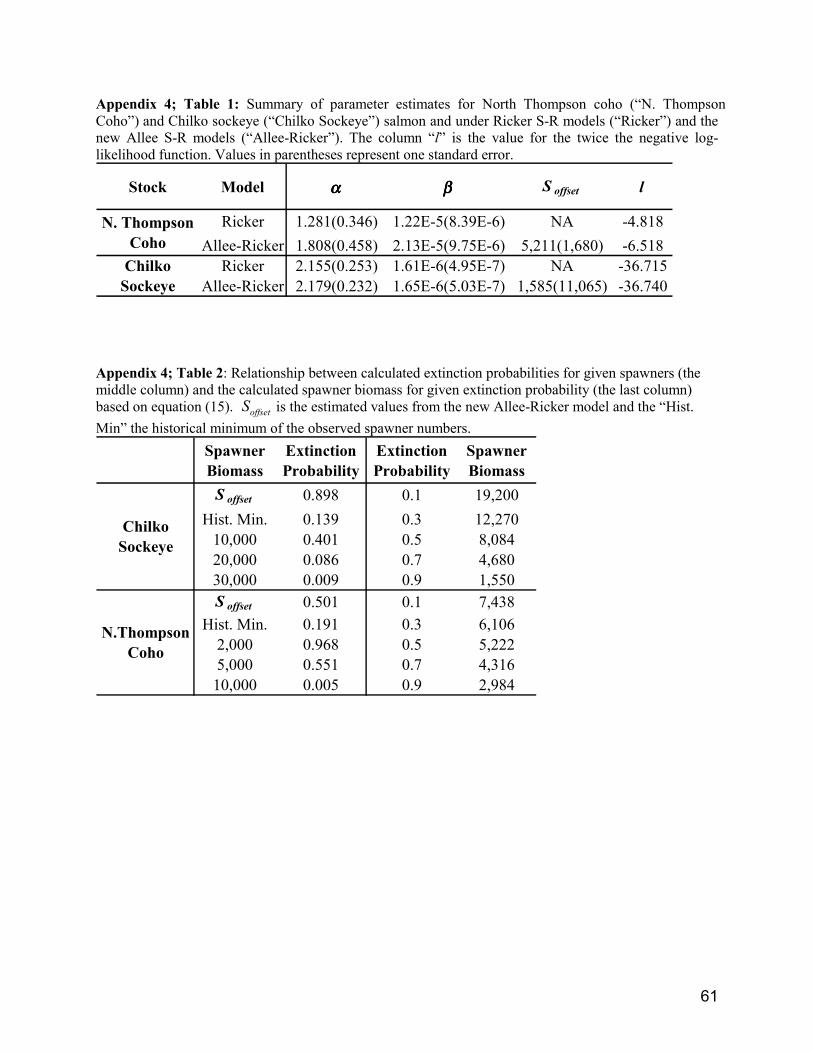
61

Appendix 4; Table 1: Summary of parameter estimates for North Thompson coho (“N. ThompsonCoho”) and Chilko sockeye (“Chilko Sockeye”) salmon and under Ricker S-R models (“Ricker”) and thenew Allee S-R models (“Allee-Ricker”). The column “l” is the value for the twice the negative log-likelihood function. Values in parentheses represent one standard error.

Stock Model αααα ββββ S offset l

Ricker 1.281(0.346) 1.22E-5(8.39E-6) NA -4.818Allee-Ricker 1.808(0.458) 2.13E-5(9.75E-6) 5,211(1,680) -6.518

Ricker 2.155(0.253) 1.61E-6(4.95E-7) NA -36.715Allee-Ricker 2.179(0.232) 1.65E-6(5.03E-7) 1,585(11,065) -36.740

Chilko Sockeye

N. Thompson Coho

Appendix 4; Table 2: Relationship between calculated extinction probabilities for given spawners (themiddle column) and the calculated spawner biomass for given extinction probability (the last column)based on equation (15). Soffset is the estimated values from the new Allee-Ricker model and the “Hist.Min” the historical minimum of the observed spawner numbers.

Spawner Biomass

Extinction Probability

Extinction Probability

Spawner Biomass

S offset 0.898 0.1 19,200Hist. Min. 0.139 0.3 12,270

10,000 0.401 0.5 8,08420,000 0.086 0.7 4,68030,000 0.009 0.9 1,550S offset 0.501 0.1 7,438

Hist. Min. 0.191 0.3 6,1062,000 0.968 0.5 5,2225,000 0.551 0.7 4,31610,000 0.005 0.9 2,984

Chilko Sockeye

N.Thompson Coho

62

Appendix 4 Figure Captions:

Figure 1: Stock recruitment relationships for North Thompson coho salmon. Solid curve is the Rickermodel (3) fit and the dashed line is the Allee Ricker model (9) fit. The straight line is the replacementline. Value “5,211” is the estimated Soffset .

Figure 2: The performance of the GA search algorithm using the North Thompson coho data. The linesfrom the top to the bottom are the worst, median, and the best values from the 100 points in everygeneration.

Figure 3. The distribution of Soffset for North Thompson coho. The vertical line is Soffset = 5,211 and thehorizontal line with arrows at both ends is the 80% confidence interval.

Figure 4: Extinction probability as a function of the North Thompson coho spawner numbers. The twovertical lines are the extinction probabilities corresponding to the estimated Soffset and the historicalminimum spawner number. The horizontal line is the calculated spawner numbers corresponding to the80% extinction probability.

Figure 5: Autocorrelation patterns for the residuals applying the standard Ricker model (plot a) and theAllee-Ricker model (plot b) to North Thompson coho data. The first order (i.e. Lag 1) autocorrelationwith the standard Ricker model was just significant since it was barely outside the 95% confidence band(dotted lines).

Figure 6: Stock recruitment relationships for Chilko River sockeye salmon. Solid curve is the Rickermodel (3) fit and the dashed line is the Allee Ricker model (9) fit. Because of the data range and scale,both lines are so close that it is difficult to distinguish them. The straight line is the replacement line.Value 1,585 close to the origin is the estimated Soffset .

Figure 7: Re-plot of Figure 6 for the part close to the origin. The solid line is the Ricker model (3) fit andthe dashed line the fit from the Allee Ricker model (9). Value “1,585” is the estimated Soffset . The onlydot in the figure is the last observed S-R data point with 17,308 spawners and 204,386 recruits.

Figure 8: The distribution of Soffset for Chilko sockeye salmon. The vertical line is Soffset =1,585 and thehorizontal line with arrows at both ends is the 95% confidence interval.

Figure 9: Extinction probability as function of the Chilko sockeye spawner numbers re-scaled so that theextinction probability is zero for the spawner biomass to be zero. The two vertical lines are the extinctionprobabilities corresponding to the estimated Soffset and the historical minimum observed spawnernumbers. The horizontal line is the calculated spawner numbers corresponding to the 50% extinctionprobability.

63

Appendix 4; Figure 1.

Appendix 4; Figure 2:

-8

-3

2

7

1 2

1 7

2 2

2 7

3 2

3 7

0 5 1 0 1 5 2 0 2 5 3 0 3 5 4 0 4 5 5 0 5 5 6 0 6 5

Ge ne ra tio ns

Obj

. Val

u

52 110

50 ,000

10 0,000

15 0,000

20 0,000

25 0,000

30 0,000

0 20 ,000 40 ,000 60 ,000 80 ,000 10 0,000

S pa w ne r

Rec

ruit

64

Appendix 4; Figure 3.

Appendix 4; Figure 4:

0 2000 4000 6000 8000 10000

0.0

0.2

0.4

0.6

0.8

1.0

Spawner

Extin

ctio

n Pr

ob.

( 5211 , 0.501 )

( 6722 , 0.19 )

( 3766 , 0.8 )

0 2000 4000 6000 8000 10000

0.0

0.05

0.10

0.15

0.20

Soffset=5,211

Soffset

Den

sity

65

Appendix 4; Figure 5.

Appendix 4; Figure 6:

0 2 4 6 8 10 12

-0.4

-0.2

0.0

0.2

0.4

0.6

0.8

1.0

Lag

ACF

a)

0 2 4 6 8 10 12

-0.4

-0.2

0.0

0.2

0.4

0.6

0.8

1.0

Lag

b)

15850

500,000

1,000,000

1,500,000

2,000,000

2,500,000

3,000,000

3,500,000

4,000,000

4,500,000

5,000,000

0 200,000 400,000 600,000 800,000 1,000,000

S pa w ne r

Rec

ruit

66

Appendix 4; Figure 7:

Appendix 4; Figure 8.

15850

50 ,000

100 ,00 0

150 ,00 0

200 ,00 0

250 ,00 0

0 5 ,000 10 ,000 15 ,000 20 ,000 25 ,000

S p aw ne r

Rec

ru

-30000 -20000 -10000 0 10000 20000 30000

0.0

0.01

0.02

0.03

Soffset=1585

Soffset

Den

sity

67

Appendix 4; Figure 9:

0 10000 20000 30000

0.0

0.2

0.4

0.6

0.8

1.0

Spawner

Extin

ctio

n Pr

ob.

( 1585 , 0.898 )

( 17308 , 0.139 )

( 8084 , 0.5 )