2005 colorado (plsc) conference handouts - terrasurv
TRANSCRIPT


What is Geodesy???Science concerned with size and shape of the Earth (Helmert 1880)Science that locates positions on the Earth and determines Earth’s gravity fieldThe branch of surveying in which the curvature of the Earth must be taken into account when determining directions and distances

What is control surveying?NGS definition-”A survey that provides coordinates (H & V) of points to which supplementary surveys are adjustedMy definition-”A survey which is performed to achieve higher than normal accuracies”
Usually adjusted from redundant measurementsHorizontal, Vertical, 3-D (GPS)

1974 Specifications
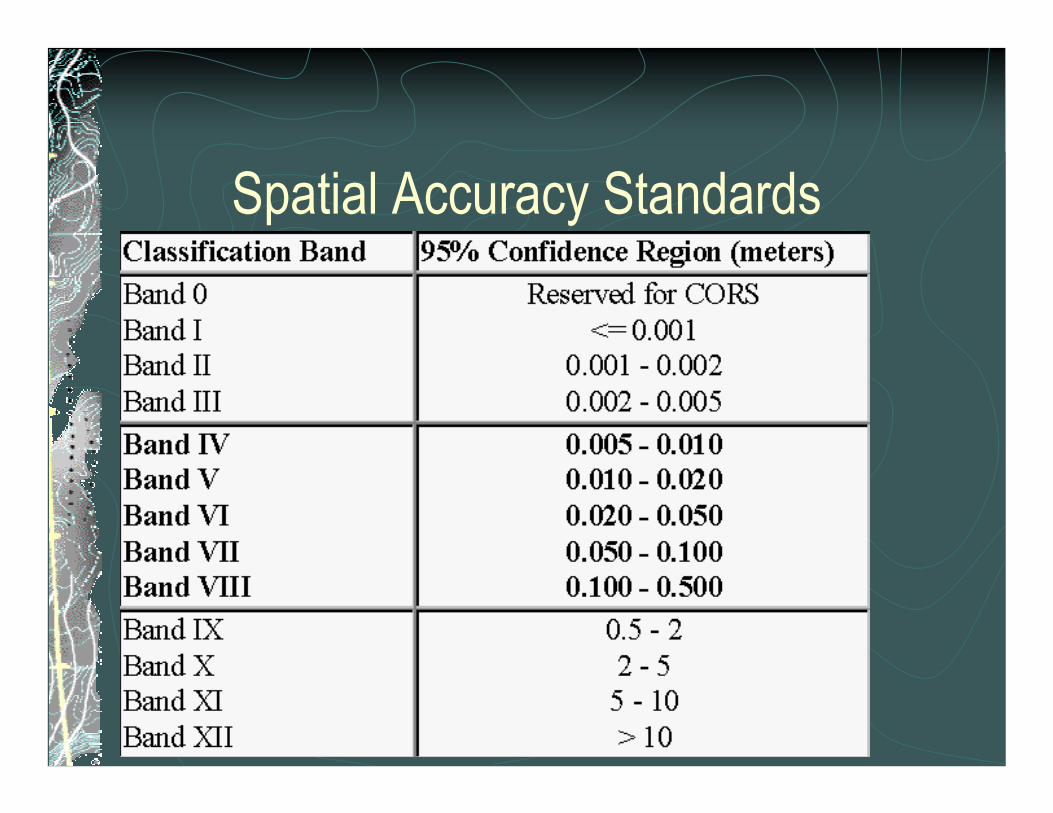
Spatial Accuracy Standards

COORDINATESOne of an ordered set of N numbers which designates the location of a point in a space of N dimensionsIn surveying and mapping, 1≤N≤3
Could also be time tagged (N=4)A coordinate is AN ESTIMATE OF THE POSITION of a pointAs more data is collected, the position is refined, coordinate changes

Coordinate Systems
ECEF - Earth Centered Earth FixedLLH - Latitude, Longitude, HeightGrid - State Plane, UTM, localHeight Systems
GeoidEllipsoid
DatumsA coordinate system needs a datum to be complete

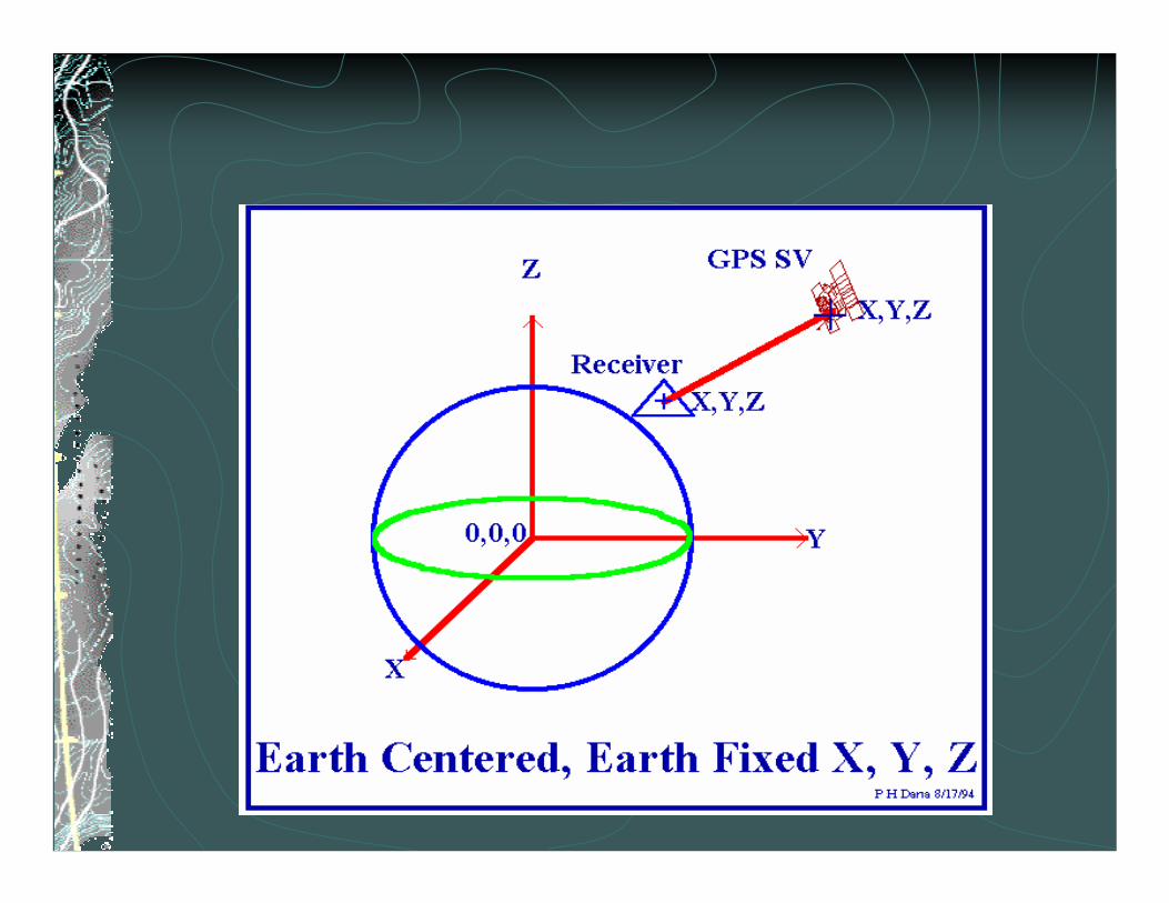
ECEF
three dimensional cartesian systemorigin at center of massused by GPS systemconvert to/from LLHcartesian geometryindependent of ellipsoid

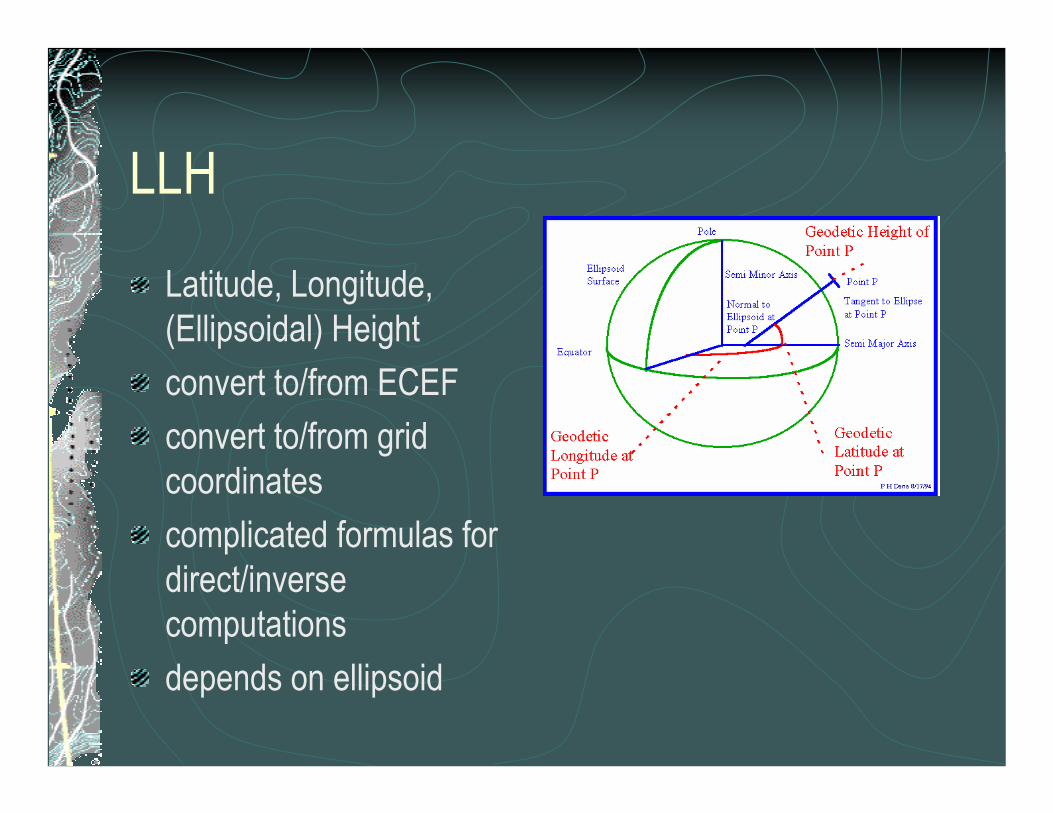
LLH
Latitude, Longitude, (Ellipsoidal) Heightconvert to/from ECEFconvert to/from grid coordinatescomplicated formulas for direct/inverse computationsdepends on ellipsoid


LLH ECEF
2 21 sinaN
e φ=
−
2
( ) cos cos( )cos sin
((1 ) )sin
X N hY N hZ e N h
λλ
+ Φ⎡ ⎤ ⎡ ⎤⎢ ⎥ ⎢ ⎥= + Φ⎢ ⎥ ⎢ ⎥⎢ ⎥ ⎢ ⎥− + Φ⎣ ⎦ ⎣ ⎦
2 22
2
a bea−
=
a=semi-major axis
b=semi-minor axis
h=height above ellipsoid


ECEF LLH
⎟⎟⎠
⎞⎜⎜⎝
⎛⎟⎠⎞
⎜⎝⎛
+−
+=Φ
−−
12
22
1 1tanhN
NeYX
Z
Must use iterative process since h depends on Φ and vice-versa
XY1tan −=λ
2 2
cosX Yh N
φ+
= −

Grid Coordinates
two dimensional - Y and X or N and Erelated to LLH, can convert back and fortheasy computationsmost systems distort distances vary in extentplane, Transverse Mercator, LambertUTM, State Plane, Local
State Plane
developed by the US Coast & Geodetic Survey (now NGS) to enable use of geodetic control by local surveyorsmathematically rigorousLambert or Transverse Mercator Projectionsmaximum 100 ppm distance distortiontransform to/from LLH

UTM
Universal Transverse Mercatordeveloped by US militaryworldwide, broken into sixty 6° zonesmaximum distance distortion 400 ppmMGRS - Military Grid Reference Systemtransform to/from LLHeasy to program into GPS receiver


Local Grid Systems
usually tangent system (plane)if origin is known, can transform to/from LLHsimplified computationsvery common, not recommended unless origin is tied to NSRS and documented

Example: City of PittsburghSelected origin based on arbitrary pointBased on USGS published NAD positions for 3 triangulation stations (done in early 1920’sExtended by triangulation, supplemented by taped baselines and astro azimuthsLocal coordinates=100,000N/100,000E

Ellipsoid
mathematical surface which closely approximates the physical shape of the earthgenerated by rotating an ellipsoid about its semi-minor axisdefined by two axes (a, b), or by one axis and the flattening (a, 1/f)geocentric or non-geocentric (“local”)

THE ELLIPSOIDMATHEMATICAL MODEL OF THE EARTH
b
a
a = Semi major axisb = Semi minor axisf = a-b = Flattening
a
N
SGRS 1980a=6,378,137 m
b=6,356,752.3141 m
1/f=298.257222101
Geoid
level surface of the gravity field which best fits mean sea levelnot a smooth mathematical surfaceaffected by gravity anomalies, such as mountains reference surface for orthometric heights


Relation between Ellipsoid and Geoid
N is the separation varies from point to pointinterpolated using geoid model
GEOID03 (North America), other regional modelsEGM96 – worldwide, but coarser than regional models

Geoid models1993, 1996, 1999, 2003Combination of gravity measurements, Astronomic Observations, DEM, and Global Geopotential ModelLatest model (2003) adds 14000+ benchmarks (GPS on benchmarks) to more accurately match the two surfaces

GEOID03


ELLIPSOID - GEOID RELATIONSHIP
H h
EllipsoidGRS80
H = Orthometric Height (NAVD 88)
N
Geoid
H = h - N
PERPENDICULAR TO ELLIPSOID
PERPENDICULARTO GEOID (PLUMBLINE)
DEFLECTION OF THE VERTICALDEFLEC99
TOPOGRAPHIC SURFACE
h = Ellipsoidal Height (NAD 83)N = Geoid Height (GEOID03)
GEOID03

GEOID03 in Colorado


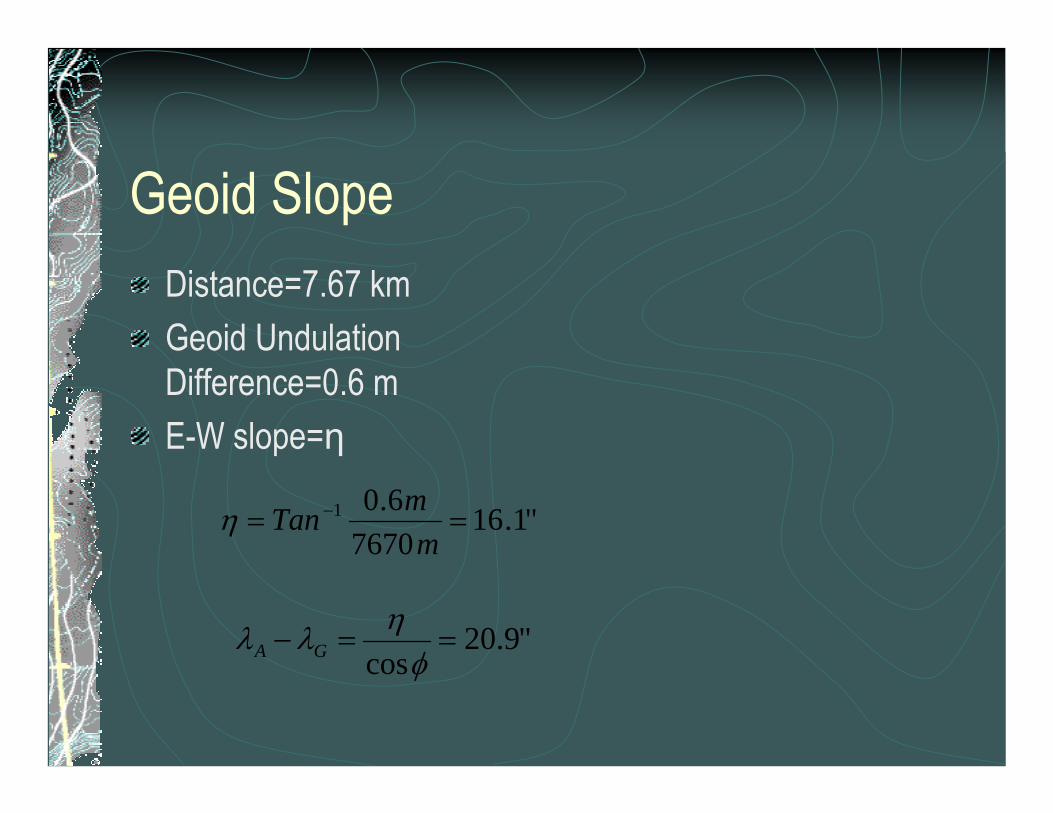
Geoid SlopeDistance=7.67 kmGeoid Undulation Difference=0.6 mE-W slope=η
"1.167670
6.01 == −
mmTanη
"9.20cos
==−φ
ηλλ GA

Observed Astronomic PositionObtained from NGS databaseStation BLACK (PID KK1879)Astronomic Observations in 1980
Latitude=39°31’04.13″ σ=0.26 ″Longitude=105°20’45.22″ σ=0.33 ″
NAD 1983 Geodetic Latitude=39°31’04.29238″Longitude=105°21’09.69043″

Astronomic minus GeodeticN-S Difference=meridian deflectionξ=ΦA-ΦG (Xi)=4.13″-4.29″=-0.16″DEFLEC99=-0.13″
E-W Difference=prime vertical deflectionη =(λA- λG)*cosΦ (Eta)=(45.22″-69.69″)*cos(39°31’04.3)"=-18.88″DEFLEC99=+18.40“
(different sign convention)

LaPlace CorrectionDefinition: The equation which expresses the relationship between astronomic azimuth and geodetic azimuth in terms of astronomic longitude, geodetic longitude, and geodetic latitudeαA-αG=(λA-λG)*sinΦ=η*tanΦDEFLEC99 provides interpolated value from model

LaPlace CorrectionAstronomic Observation BLACK->VA 9700 (BERGEN)
September 1977: 347°31’48.58" σ=1.5 “October 1977: 347°31’51.48" σ=1.5 “Mean= 347°31’50.03"
αA-αG=(λA-λG)*sinΦαG= αA- 24.47" * sin(39°31’04.29 ")αG= 347°31’34.46 "Inverse= 347°31’32.19"

LaPlace CorrectionComputed Value=-15.57"DEFLEC99=-15.18"
Uses a geoid modelFor this purpose, GEOID99 is the same as GEOID03


Ellipsoids used in the USClarke 1866
a=6,378,206.4 m b=6,356,583.8 mUsed for New England Datum, NAD, and NAD 1927
Geodetic Reference System 1980 (GRS80)a=6378137 m b=6,356,752.3141 mUsed for NAD 1983
World Geodetic System 1984 (WGS 1984)a=6378137 m b=6,356,752.3142MilitaryAlso a datum


THE GEOID AND TWO ELLIPSOIDS
GRS80-WGS84
CLARKE 1866
GEOID
Earth MassCenter
Approximately236 meters

Datum“Any quantity or set of such quantities that may serve as a reference or basis for calculation of other quantities”Geodetic Datum-”A set of constants specifying the coordinate system used for geodetic control, i.e., for calculating coordinates of points on the Earth”

Defining a Datum5 parameter-horizontal location (2), azimuth, and size of ellipsoid (2)
Used for older datums before geocentric datums were possible
8 parameter-spatial location (3), spatial orientation (3), and size of ellipsoid (2)
Used for modern datumsOther possibilities

Early US Horizontal DatumsNew England Datum – based on astronomic position of PRINCIPIO in Maryland (1879)Position transferred (through triangulation network) to MEADES RANCH (Kansas), later renamed US Standard Datum in 1901 and North American Datum (NAD) in 1913

Meades Ranch, Kansas

Horizontal Control - 1901

Horizontal Control - 1927
NAD 1927Clarke 1866 ellipsoidOrigin at MEADES RANCH, KS
Astronomic position, but not measured at stationAssumed geoid separation=0 at originUsed all data observed up to that timeNon Geocentric (best fit to North America)

NAD 1927 problemsLack of geoid model led to scale problems in the western USLack of simultaneous adjustment
Data observed later forced to fitEDM’s used by surveyors were more accurate than the network in many cases

NAD 1983 1986
readjustment by NGS of all NSRS data geocentric, GRS 1980 ellipsoid, same parameters (nominally) as WGS 1984contained small (up to 1 m) distortionsfixed to the North American continentBased on VLBI, SLR, Doppler

NAD 1983 199X
NAD 1983 199Xbased on HARN surveysdifferent states have different year suffixesimprovement on NAD 1983 1986, with space based technologiesSame Ellipsoid/Same Datum-improved positions
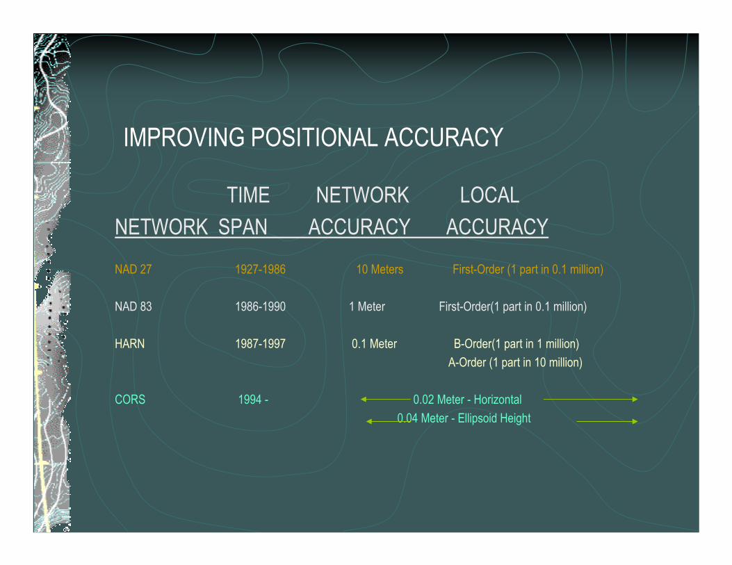
IMPROVING POSITIONAL ACCURACY
TIME NETWORK LOCAL NETWORK SPAN ACCURACY ACCURACY
NAD 27 1927-1986 10 Meters First-Order (1 part in 0.1 million)
NAD 83 1986-1990 1 Meter First-Order(1 part in 0.1 million)
HARN 1987-1997 0.1 Meter B-Order(1 part in 1 million) A-Order (1 part in 10 million)
CORS 1994 - 0.02 Meter - Horizontal 0.04 Meter - Ellipsoid Height
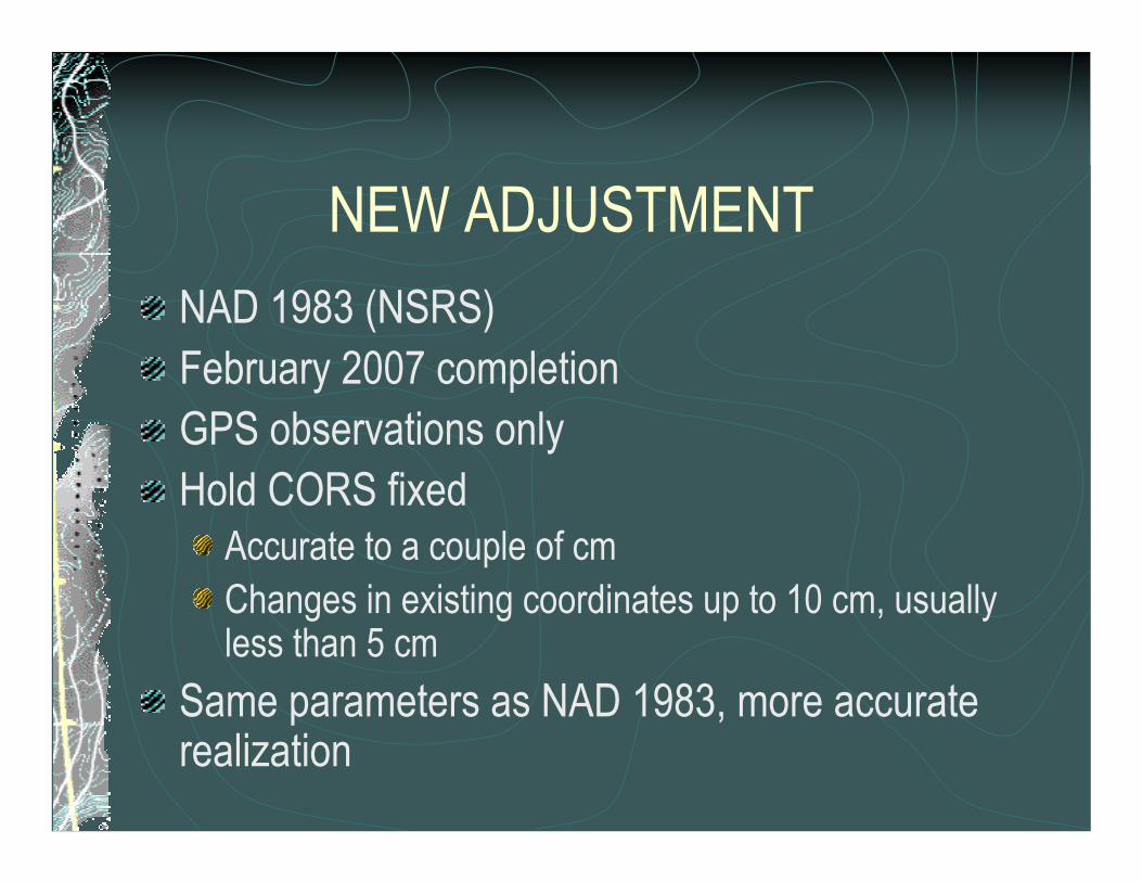
NEW ADJUSTMENTNAD 1983 (NSRS)February 2007 completionGPS observations onlyHold CORS fixed
Accurate to a couple of cmChanges in existing coordinates up to 10 cm, usually less than 5 cm
Same parameters as NAD 1983, more accurate realization

WGS 1984Created by Defense Department (third in a series, replaced WGS 1972)Intended to be the same as NAD 1983, used same ellipsoid (very slight difference)DIFFERENT REALIZATION THAN NAD 1983
“realized” by coordinates of GPS tracking stationsNOT GENERALLY ACCESSIBLE to non-military users

WGS 1984GPS satellites use this systemEarly realizations by precise point positioning Newer Realizations based on ITRFPeriodically “redefined” by being made to coincide with ITRF at a certain epoch
WGS 1984 (G873)=ITRF 1994 1997.0WGS 1984 (G1150)=ITRF 2000 2001.0 (current)
Broadcast by GPS satellites in the ephemerisWill change again due to plate tectonics

WORLD GEODETIC SYSTEM 1984TR8350.2 World Geodetic System 1984 - It’s Definition andRelationships with Local Geodetic Systems(http://www.nima.mil/GandG/pubs.html)
DATUM = WGS 84(G730)Datum redefined with respect to the International TerrestrialReference Frame of 1992 (ITRF92) +/- 20 cm in each component (Proceedings of the ION GPS-94 pgs 285-292)
DATUM = WGS 84(G873)Datum redefined with respect to the International TerrestrialReference Frame of 1994 (ITRF94) +/- 10 cm in each component (Proceedings of the ION GPS-97 pgs 841-850)
DATUM = WGS 84RELEASED - SEPTEMBER 1987BASED ON OBSERVATIONS AT MORE THAN 1900 DOPPLER STATIONS
DATUM = WGS 84(G1150)Datum redefined with respect to the International TerrestrialReference Frame of 2000 (ITRF00) +/- 2 cm in each component (Proceedings of the ION GPS-02 pgs xxx-xxx) http://164.214.2.59/GandG/sathtml/IONReport8-20-02.pdf

MY SOFTWARE SAYS I’M WORKING IN WGS-84
Project tied to WGS-84 control points obtained from the Defense Department -- Good Luck!
You’re really working in the same reference frame as your control points -- NAD 83?
Unless you doing autonomous positioning (point positioning +/- 6-10 meters) you’re probably NOT in WGS-84

I NEED TO TRANSFORMBETWEEN WGS 84 AND NAD 83
Federal Register Notice: Vol. 60, No. 157, August 15, 1995, pg. 42146“Use of NAD 83/WGS 84 Datum Tag on Mapping Products”

ITRF XX
International Terrestrial Reference Frame, where XX is the epoch of the system, for example ITRF 00Most accurate system in use – cm level accuracyworldwide, not fixed to any continental plateALL NAD 1983 coordinates have velocity components in ITRFconstantly being refined by I

ITRFSlightly different ellipsoid, basically same as GRS 1980Updated every few years, latest is ITRF 2000, ITRF 2004 is due out soonPlate Tectonics are accounted for
No single fixed pointAll points have velocities

NAD 83 and ITRF
ITRFNAD 83
Earth MassCenter
2.2 m (3-D)dX,dY,dZ
GEOID


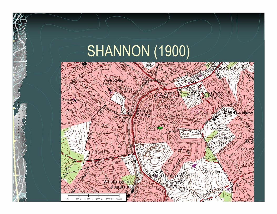
SHANNON (1900)

SHANNONNAD 1983 (1992)
40º21´33.39838" N/80º01´25.03102" WNAD 1983 (1995)
40º21´33.39907" N/80º01´25.03264" WNAD 1983 (1986)
40º21´33.40178" N/80º01´25.03959" WNAD 1927
40º21´33.15538" N/80º01´25.85590" WNAD
40º21´33.53" N/80º01´26.95" W

Inverses from HARN (1992) positionNAD 1983 1995
0.044 m (0.14 ft) 299ºNAD 1983 1986
0.228 m (0.75 ft) 297ºNAD 1927
20.86 m (68.44 ft) 249ºNAD
45.46 m (149.15 ft) 275º
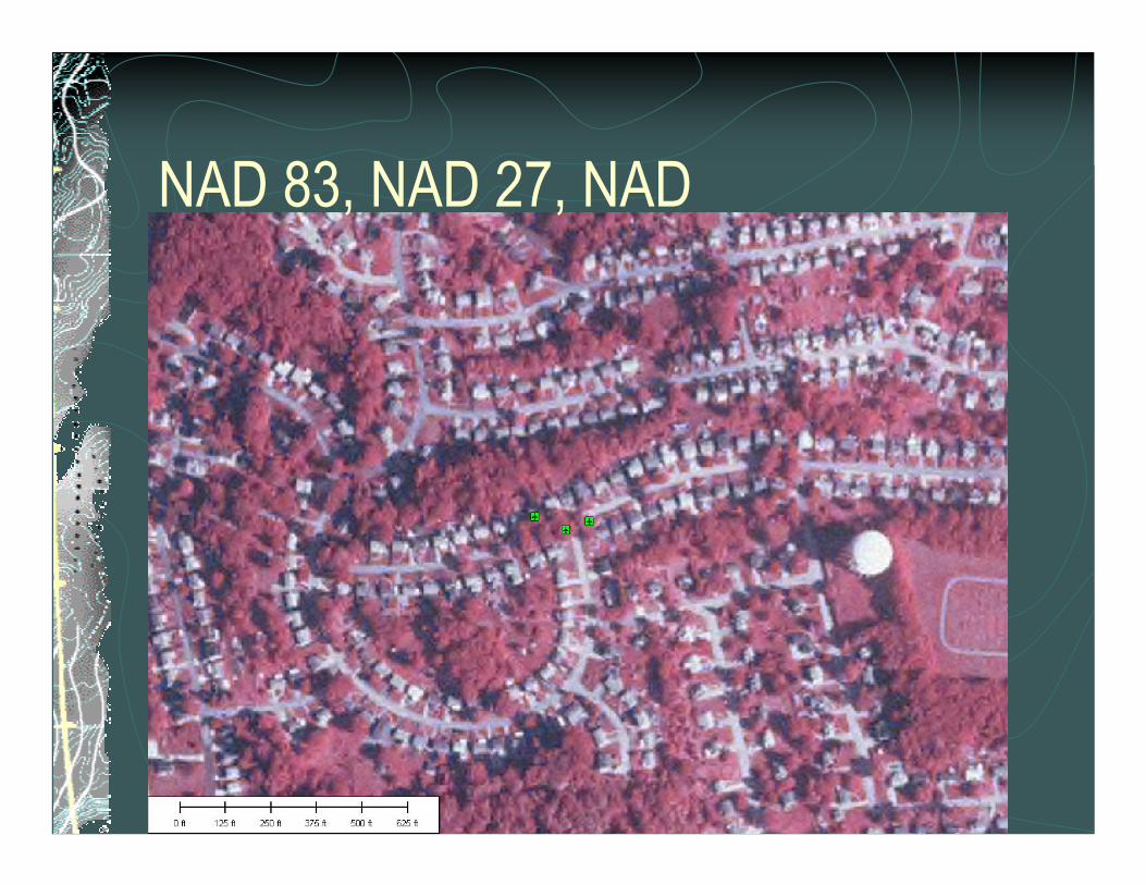
NAD 83, NAD 27, NAD

NAD 1983 versus NAD 1927Clarke 1866Origin=MEADES RANCH25,000 stationsSeveral hundred taped baselinesSeveral hundred azimuths
GRS 1980Origin=Center of earth mass250,000 stations30,000 EDM baselines5,000 azimuths


NADCON DESIGNED TO SATISFY THE MAJORITY OF THE “IDEAL METHOD” DESIGN AND
IS DEFINED AS THE NATIONAL STANDARD.
DESIGN CRITERIA:Relies only on NGS archived data existing in both NAD 27 and NAD 83Provides consistent results, both forward and inverseFastNot tied to NGS Data BaseSmall - Fit on PCAccurate
15 cm (1 sigma) in Conterminous U.S. NAD 27 - NAD 83(1986)
5 cm (1 sigma) per State/Region NAD 83 (1986) - HARN
Federal Register Notice: Vol. 55, No. 155, August 10, 1990, pg. 32681“Notice to Adopt Standard Method for Mathematical Horizontal Datum Transformation”

NADCONN = +0.123448 = -1.87842
N = +0.122498 = -1.88963
N = +0.124238 = -1.81246
N = +0.125688 = -1.83364
N = +0.124498 = -1.88905
N = +0.124998 = -1.86543
N = +0.126408 = -1.85407
N = +0.124388 = -1.86547
N = +0.123548 = -1.8594
N = +0.124318 = -1.86291
N = +0.124418 = -1.83879


Vertical Datums
NGVD 1929 - formerly known as Mean Sea Levelbased on constraining local sea level at various (21 US, 5 Canada) tide stationsNAVD 1988 - more accurate, consistent systembased on sea level at one tide station between US and Canada

Vertical Datums
GEOID03 model works best when using GRS 80 and NAVD 1988Local datums - often based on local sea level, need to exercise caution when usingUSGS benchmarks do not, in general, have NAVD 1988 heightscan use VERTCON to convert NGVD 1929 to NAVD 1988
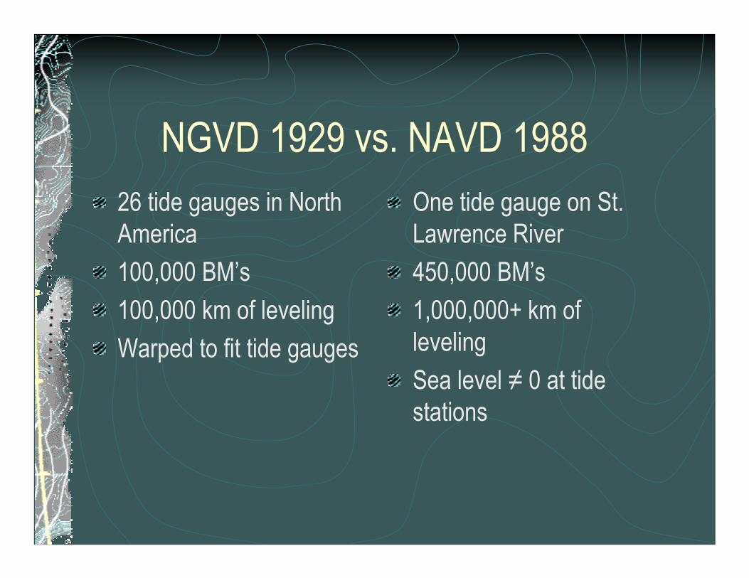
NGVD 1929 vs. NAVD 198826 tide gauges in North America100,000 BM’s100,000 km of levelingWarped to fit tide gauges
One tide gauge on St. Lawrence River450,000 BM’s1,000,000+ km of levelingSea level ≠ 0 at tide stations

NGVD 29 and NAVD 88

METADATA METADATA IS DATA ABOUT DATA
DATUMS NAD 27, NAD 83(1986), NAD83 (199X), NAD83(CORS96) NGVD29, NAVD88
UNITS Meters, U.S. Survey Feet, International Feet, Chains, Rods, Pole
ACCURACY A, B, 1st, 2nd, 3rd, 3cm, Scaled

METADATA??Horizontal Datum??
Plane Coordinate Zone ??
Units of Measure ??
How Accurate ??
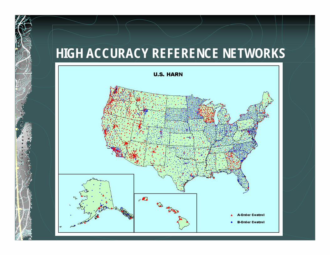
HIGH ACCURACY REFERENCE NETWORKS


Wide Area Augmentation System (WAAS)
FAA programProvides corrections via geosynchronous satelliteBased on ITRF NOT NAD 1983

Earth Center
a’
b’
a
bc
dc’
d’GEODETIC
vs. GRID DISTANCE
ab > a’b’
cd < c’d’
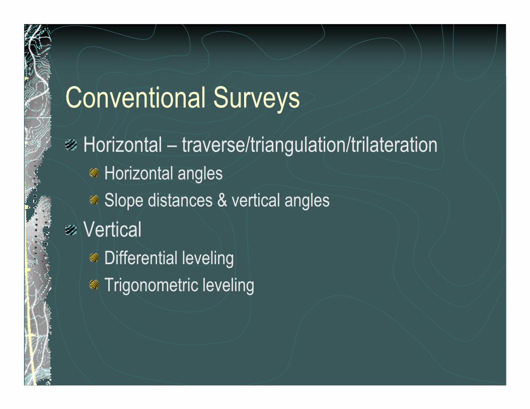
Conventional SurveysHorizontal – traverse/triangulation/trilateration
Horizontal angles Slope distances & vertical angles
VerticalDifferential levelingTrigonometric leveling
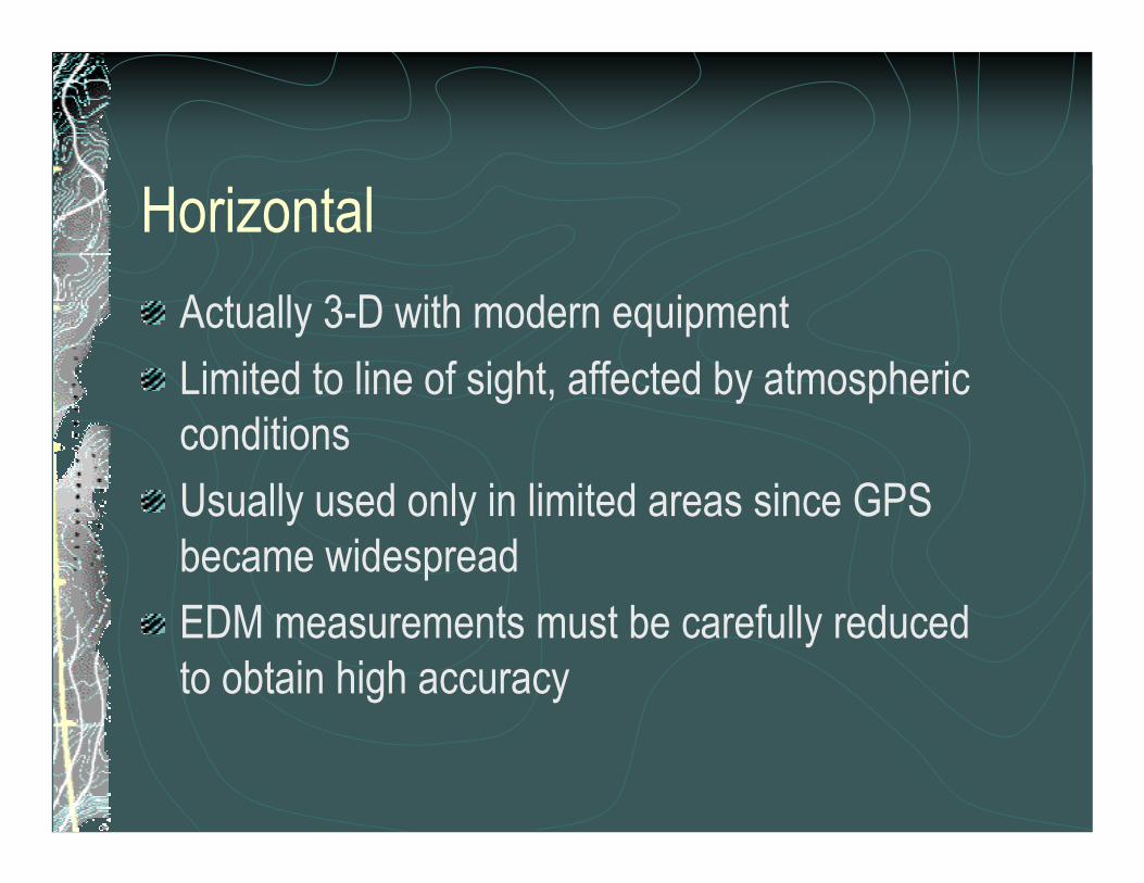
HorizontalActually 3-D with modern equipmentLimited to line of sight, affected by atmospheric conditionsUsually used only in limited areas since GPS became widespreadEDM measurements must be carefully reduced to obtain high accuracy

Applicable standardsStandards and Specifications for Geodetic Control Networks – 1984
Mainly for networks covering large areas-good leveling specs
US Army Corps of Engineers – Geodetic and Control Surveying – very appropriateCaltrans
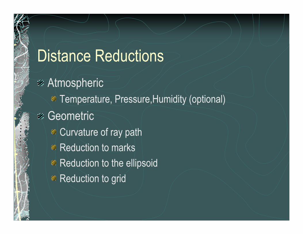
Distance ReductionsAtmospheric
Temperature, Pressure,Humidity (optional)Geometric
Curvature of ray pathReduction to marksReduction to the ellipsoidReduction to grid

Atmospheric Correction
Ambient Refractive IndexT=temperature in °K (°C+273°)P=pressure in millibarsE=partial water vapor in millibarsNg=Group Refractive Index (depends on instrument
T*3.709e*41.8-p*N=N g

How Accurate do we need to be?
)dTe*11.3+p*3.709
N-(T1=dN g
2T
dPT*3.709
N=dN gp
deT
11.3=dN e _
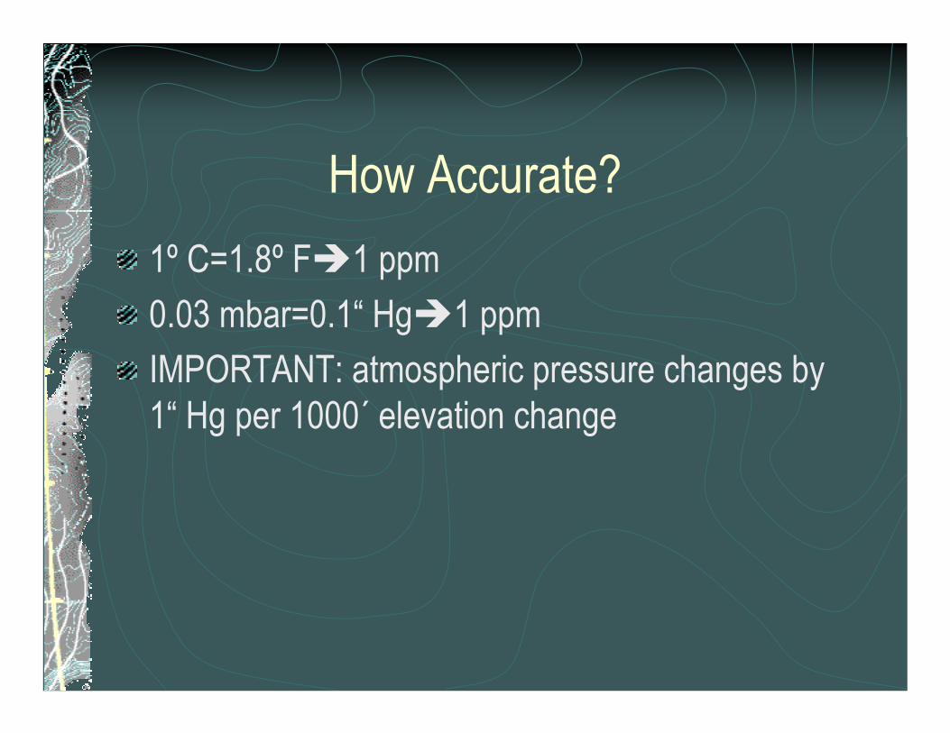
How Accurate?1º C=1.8º F 1 ppm0.03 mbar=0.1“ Hg 1 ppmIMPORTANT: atmospheric pressure changes by 1“ Hg per 1000´ elevation change

By distanceShort (<3 km)
2 ppm acceptable error±1° C (±1.8°F)±3 mb (±0.1” Hg)Humidity ignored
Medium (or high accuracy short lines)1 ppm acceptable error<±1°C±1 mb (±0.03” Hg)Sling psychrometer (or electronic humidity device)Measure at both ends

PPM correction accuracyBiggest limitation to high accuracy over longer linesSome newer total stations have PPM on-board
BUT, this only samples at the standpointIf large difference in elevation is present, may not accurately reflect line conditionsBoth temperature and pressure vary spatially as well as by elevation

Altitude effectsTemperature lapse rate (standard)
0.0065° C per meterCan vary due to temperature inversion/ground heating
Pressure lapse rate (standard)0.115 mb per meter (~1” per thousand feet)More consistent than temperature

Geometric CorrectionsSlant range from EDM to reflector
First reduced for any non colinear EDM/reflectorReduced to mark-to-mark (can skip this step)Reduced to ellipsoid (not sea level!)Reduced to grid
Depends on what value is expected by the software


ExamplePoint at Pittsburgh
03016CB 03016CALatitude=40º26'45.98795" N Latitude=40º26'30.67851" NLongitude=80º02'01.48205" W Longitude=80º00'43.34624" WNAVD88=337.762 m NAVD88=219.493 mEllip H=303.938 m Ellip H=185.695 mGeoid 2003 N=-33.825 m Geoid 2003 N=-33.798 m


On Board ppm=+18.61 ppmActual value=+18.64 ppm (using T & P from airports)Computed ppm at forepoint=+14.97 (due to elevation difference)Mean PPM correction=+16.81
Total Station Observations:Zeiss S10, from 03016CB to 03016CA at 10:45 AM on 7/23/2003HI=1.435 m HT=2.100 mAtmospheric conditions:At KAGC: T=64°F DP=63°F RH=96.5% P=29.90”At KPIT: T=64.9°F DP=62.1°F RH=90.6% P=29.91”Convert 29.90” SLP to station pressure=28.73” hg Zeiss on-board sensors: 67° F/28.7” hg

Observations:Direct: ZD=93°32’59.3” SD=1904.6573 mReverse: ZD=266°27’03.6” SD=1904.6585 mMean: ZD=93°32’57.9” SD=1904.6579 m
DM=1904.6579 m (mean, corrected for T and P in S10)DR=1904.6225 m (raw, uncorrected for T and P)DEDM=1904.6545 m (corrected for actual conditions)
This latter value, DEDM, is the ray path length, corrected for atmospheric delay.

reduce Z to mark-to-mark
dZ)h-h(
G
ththt sin×≅Ω
( )6545.1904
)"9.57'3293sin(435.11.2 °×−≅Ω
=0.000348475 radians =0°01 11.9
Ω+Z=Z thG
ZG = 93°32 57.9 +0°01 11.9
ZG = 93°34 09.8

Reduce D to mark-to-mark
cos
edmG 2
edm redm rG2
GG
d=d2 ( - )( - ) h hh h1+ - Z
dd×
×
( ) ( ) ( )2
2
1904.6545
1.435 2.1 2 1.435 2.11 cos 93 34 '09.8"
1904.6545 1904.6545
Gd =− × −
+ − × °
dG=1904.6958 m

Comparison with GPSGPS processing usually gives mark-to-markObserved 2 30 minute sessionsSession 1=1904.6955 mSession 2=1904.6979 mMean=1904.6967 mEDM=1904.6958Difference=0.0009 m (0.47 ppm)

Reduce mark-to-mark to the ellipsoid22
2 1Ge
1 2
- ( - )H Hdd H H(1+ ) (1+ )R R
=×
185.695 303.9381904.6958185.695 303.9386371000 6371000
22
e- ( - )
d(1+ ) (1+ )
=×
de=1900.9490 m

Which radius of curvature?The radius of curvature is used to reduce to the ellipsoidStandard practice is to use a mean value (6,371,000 m or 20,906,000 US Feet)What effect does this have?


M=Radius of Curvature in Meridian
⎪⎭
⎪⎬⎫
⎪⎩
⎪⎨⎧
×
×
)e-(1)e-(1a=M
22 3/2
2
φsin
( )6378137 0.00669438002290
0.00669438002290 40º26'45.98795" sin3/22
(1- )M =(1- )
⎧ ⎫×⎪ ⎪⎨ ⎬
×⎪ ⎪⎩ ⎭
M=6362307.7 m

N=Radius of Curvature in the Prime Vertical
⎪⎭
⎪⎬⎫
⎪⎩
⎪⎨⎧
×× φφ sincos 2222
2
b+aa=N
( ) ( )6378137
40º26'45.98795" 40º26'45.98795"6378137 cos 6356752.3141 sin
2
2 2 2 2N =
+
⎧ ⎫⎪ ⎪⎨ ⎬
× ×⎪ ⎪⎩ ⎭
N=6387140.8 m

Radius of Curvature in azimuth of line
⎭⎬⎫
⎩⎨⎧
×××
AN+AMNM=R 22A
cossin
( ) ( )6362307.7 6387140.8
6362307.7 104°22'36.14" 6387140.8 104°22'36.14"sin cosA 2 2=R +⎧ ⎫×⎪ ⎪⎨ ⎬× ×⎪ ⎪⎩ ⎭
RA=6385604.2 m

Reduction to ellipsoid185.695 303.9381904.6958
185.695 303.9386385604.2 6385604.2
22
e- ( - )
d(1+ ) (1+ )
=×
de=1900.9491 m (difference of 0.0001 m, 0.05 ppm)(negligible, OK to use mean value)

Reduction to gridDepends on grid systemScale varies N-S in LambertScale varies E-W in transverse MercatorShould be applied to the ellipsoidal distance

UTM Zone 170.99968265 (317 ppm) at 03016CB0.99968641 (314 ppm) at 03016CAMean=0.99968453Grid distance=1900.349 m

Trigonometric Height DifferenceOne way only (not reciprocal)No curvature and refraction correction:
( )cosG GH d Z∆ = ×
( )1904.6958 cos 93°34'09.8"H∆ = ×
H=-118.581 m

Curvature & Refraction estimated
cos( ) sin 2GG GG
1- kH = Z +( ) ( )d d Z2 R∆ × × ×
×
K can vary, assumed to be 0.13( )0.131904.6958 cos(93 34 '09.8") 1904.6958 sin 93 34 '09.8"
637100021-H = +( ) ( )
2∆ × ° × × °
×
H=-118.581+0.247 =-118.324 m

Refraction Coefficient, kCan vary from –1.0 to +1.0, especially if grazing the groundMean value of +0.13 often assumedKnowing actual DE, we can solve for k
( )( )( )( )2
cos0.5
sinG G
G G
R H d Zk
d Z
× ∆ − ×= −
×
=-0.050

Refraction CoefficientSimultaneous (or near-simultaneous) observations will eliminate the uncertaintyAccurate work should not use one-way observationsEspecially important where the line of sight is affected by heat waves

AzimuthsFrom backsight (i.e. intervisible pair)From Astronomic ObservationsFrom GPS (basically same as backsight method)

Astronomic AzimuthCan use sun, moon, planets, starsMust have accurate timeMust have accurate ephemerisSun and moon can be observed in daylightOther objects require night observations10” easily achieved, ±2” with advanced equipment and procedures

Astronomical triangle

Astronomical triangleUnknown=Azimuth to star Knowns=latitude, longitude, declination, right ascension, timeOnce we solve the azimuth to the star, apply the horizontal angle to get the azimuth to the mark

PositionLatitude and longitude should be astronomic rather than geodeticDifference between astronomic and geodetic coordinates is the deflection of the verticalUsually small and can frequently be ignoredShould be considered for highest accuracy if not using Polaris

TimeUTC=uniform scale, broadcast by radio
Changes by integer second steps when necessaryUT1=measure of actual rotation of earth
Within ±0.9 s of UTC, correction=DUT1UT1=UTC+DUT1DUT1 is broadcast with signal, also predictions are available
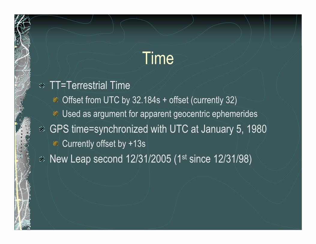
TimeTT=Terrestrial Time
Offset from UTC by 32.184s + offset (currently 32)Used as argument for apparent geocentric ephemerides
GPS time=synchronized with UTC at January 5, 1980Currently offset by +13s
New Leap second 12/31/2005 (1st since 12/31/98)

Ephemeris DataNeed Local Hour Angle (LHA) of the object at the instant of observationSome ephemerides directly list the Greenwich Hour Angle (GHA)
LHA=GHA+λOthers list Right Ascension (RA)
LHA=Local Apparent Sidereal Time (LAST)-RALAST=computed from GMST, equation of equinoxes, and longitude

UT LASTLookup GAST for 0h and 24h UTInterpolate for actual UT of observationSubtract west longitude (convert to HHMMSS)This is the hour angle of the vernal equinox (origin of right ascension system)Add/subtract right ascension of object to get local hour angle

Azimuth equation
TanAh
h=
−sin( )
cos tan sin cos( )Φ Φδ
Where h is the local hour angleδ is the declinationΦ is the (astronomic) latitude

Laplace CorrectionConverts astronomic azimuth to geodetic azimuthη=deflection of the vertical in the meridianΦ=latitude
η φ* tan

Astronomic Azimuth ReductionsCompute UT1 from UTC (apply DUT1)(compute TT if necessary) interpolate ephemeris to obtain right ascension and declinationObtain Greenwich Apparent Sidereal Time (GAST)Compute Local Apparent Sidereal Time (LAST)Compute hour angleSolve for azimuth of objectApply angle measured angle right to get azimuth to markApply Laplace correction & grid convergence (if needed)

Solar and PolarisCan use online ephemerides(www.cadastral.com) to obtain GHA directly and declination (interpolate for UT of observation)LHA (local hour angle)=GHA-west longitudeProper leveling is VERY IMPORTANT-not corrected by D&RCauses error which is a function of elevation angle

Solar Azimuth Errors
4”4”7”1’15”10” longitude
2”7”19”0”10” latitude
6”6”11”1’53”1s time
±6 hr±4 hr±2 hrNoonerror
Decl=+23°Lat=30°

Lunar AzimuthSame steps, but must compute topocentricvalues for right ascension and declination rather than geocentricInterpolate for R.A and Decl. using polynomialsOften easier to use-no filter requiredCorrect for semi-diameter (same procedure as for sun)

Simulated Traverse14 Stations, 500 m to 1500 m spacing1 intersection station availableEDM shot both ways


Adjustment 1Two control points, one at each endNo azimuth control5” angular accuracy, 10” vertical0.005 m ± 5 ppm EDM

2-D and 1-D Station Confidence Regions (95.000 and 95.000 percent):STATION MAJOR SEMI-AXIS AZ MINOR SEMI-AXIS VERTICAL------------ --------------------- --- ------------------- --------------------00002 0.060 147 0.016 0.05800003 0.103 147 0.020 0.06900004 0.131 147 0.023 0.07600005 0.145 147 0.025 0.08200006 0.144 147 0.027 0.08300007 0.137 146 0.029 0.08200008 0.125 147 0.033 0.08100009 0.091 144 0.034 0.07900010 0.047 116 0.032 0.07100011 0.039 67 0.023 0.06600012 0.037 68 0.020 0.06000013 0.031 68 0.016 0.055

Adjustment 2Two control points at west endOpen traverse5” angular accuracy, 10” vertical0.005 m ± 5 ppm EDM

2-D and 1-D Station Confidence Regions (95.000 and 95.000 percent):STATION MAJOR SEMI-AXIS AZ MINOR SEMI-AXIS VERTICAL------------ --------------------- --- ------------------- --------------------00002 0.000 0 0.000 0.06200003 0.044 149 0.011 0.07800004 0.102 148 0.016 0.09200005 0.179 148 0.020 0.10700006 0.264 148 0.023 0.11900007 0.328 148 0.025 0.12400008 0.369 145 0.030 0.12600009 0.457 146 0.031 0.13300010 0.579 148 0.033 0.14300011 0.665 148 0.035 0.14800012 0.676 141 0.063 0.15200013 0.696 134 0.110 0.15500014 0.746 125 0.174 0.165

Adjustment 3Two control points at each end of traverseClosed traverse5” Angular Accuracy, 10” vertical0.005 m ± 5 ppm EDM

2-D and 1-D Station Confidence Regions (95.000 and 95.000 percent):STATION MAJOR SEMI-AXIS AZ MINOR SEMI-AXIS VERTICAL------------ --------------------- --- ------------------- --------------------00002 0.000 0 0.000 0.05700003 0.035 148 0.011 0.06700004 0.065 147 0.016 0.07400005 0.090 147 0.019 0.07700006 0.105 147 0.021 0.07600007 0.107 146 0.023 0.07400008 0.102 146 0.026 0.07300009 0.077 142 0.026 0.06800010 0.041 117 0.025 0.05400011 0.031 63 0.016 0.04400012 0.018 63 0.011 0.03000014 0.000 0 0.000 0.058

Adjustment 4Two control points at each endClosed traverse5” angular accuracy, 10” vertical0.005 m ± 5 ppm EDMIntersection station with unknown coordinates sighted at ends and in middle

2-D and 1-D Station Confidence Regions (95.000 and 95.000 percent):STATION MAJOR SEMI-AXIS AZ MINOR SEMI-AXIS VERTICAL------------ --------------------- --- ------------------- --------------------00002 0.000 0 0.000 0.05800003 0.034 148 0.011 0.06900004 0.064 146 0.015 0.07600005 0.088 147 0.018 0.08200006 0.102 146 0.021 0.08300007 0.105 146 0.023 0.08200008 0.101 146 0.024 0.08100009 0.077 142 0.025 0.07900010 0.040 119 0.024 0.07100011 0.030 62 0.016 0.06600012 0.017 63 0.011 0.06000013 0.000 0 0.000 0.05500015 0.250 124 0.188 0.000

Adjustment 5Two control points at each endClosed traverse5” angular accuracy, 10” vertical0.005 m ± 5 ppm EDMIntersection station with unknown coordinates sighted from every setup
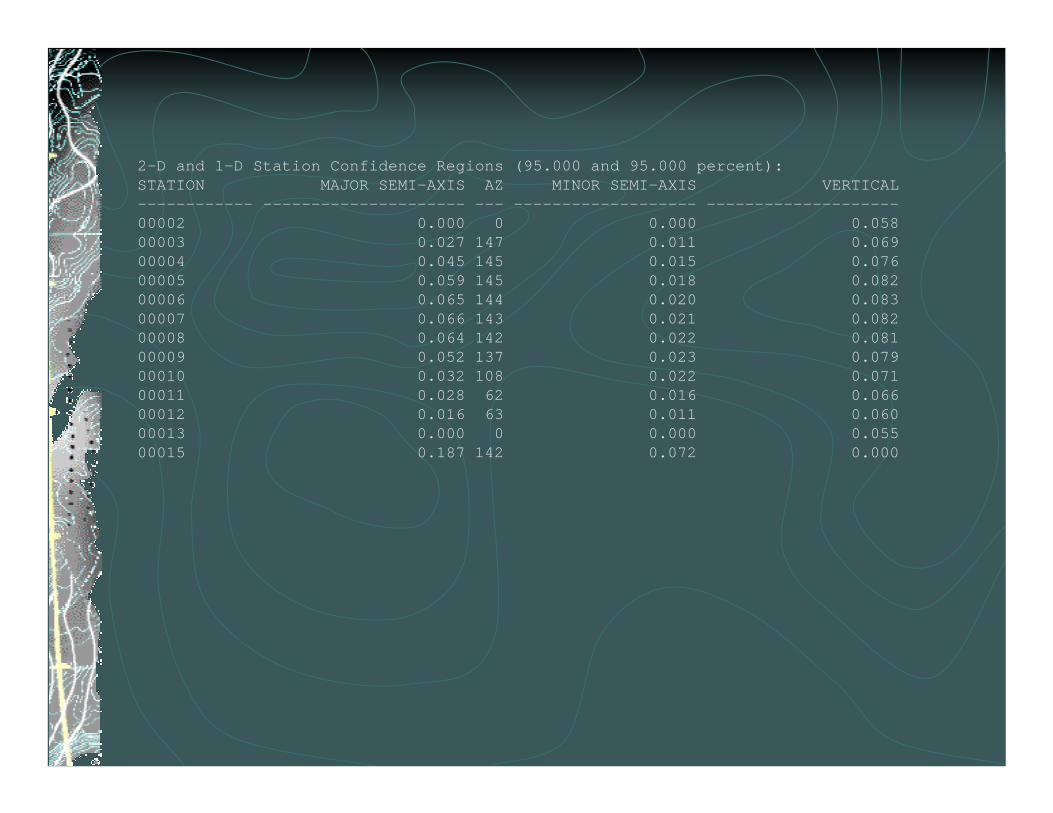
2-D and 1-D Station Confidence Regions (95.000 and 95.000 percent):STATION MAJOR SEMI-AXIS AZ MINOR SEMI-AXIS VERTICAL------------ --------------------- --- ------------------- --------------------00002 0.000 0 0.000 0.05800003 0.027 147 0.011 0.06900004 0.045 145 0.015 0.07600005 0.059 145 0.018 0.08200006 0.065 144 0.020 0.08300007 0.066 143 0.021 0.08200008 0.064 142 0.022 0.08100009 0.052 137 0.023 0.07900010 0.032 108 0.022 0.07100011 0.028 62 0.016 0.06600012 0.016 63 0.011 0.06000013 0.000 0 0.000 0.05500015 0.187 142 0.072 0.000

Adjustment 6Two control points at each endClosed traverse5” angular accuracy, 10” vertical0.005 m ± 5 ppm EDMIntersection station with known coordinates sighted from every setup
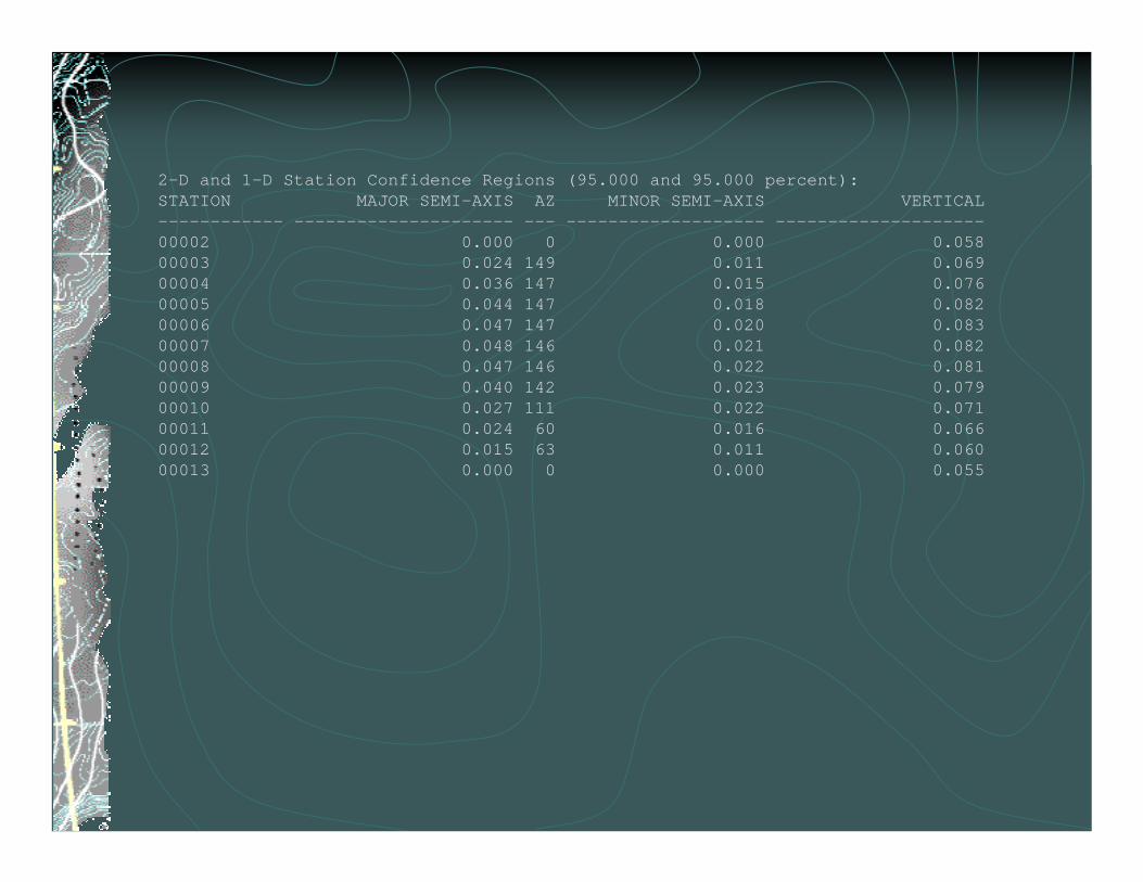
2-D and 1-D Station Confidence Regions (95.000 and 95.000 percent):STATION MAJOR SEMI-AXIS AZ MINOR SEMI-AXIS VERTICAL------------ --------------------- --- ------------------- --------------------00002 0.000 0 0.000 0.05800003 0.024 149 0.011 0.06900004 0.036 147 0.015 0.07600005 0.044 147 0.018 0.08200006 0.047 147 0.020 0.08300007 0.048 146 0.021 0.08200008 0.047 146 0.022 0.08100009 0.040 142 0.023 0.07900010 0.027 111 0.022 0.07100011 0.024 60 0.016 0.06600012 0.015 63 0.011 0.06000013 0.000 0 0.000 0.055

Adjustment 7Two control points at each endClosed traverse1.4” angular accuracy, 5” vertical0.001 m ± 2 ppm EDMNo intersection station

2-D and 1-D Station Confidence Regions (95.000 and 95.000 percent):STATION MAJOR SEMI-AXIS AZ MINOR SEMI-AXIS VERTICAL------------ --------------------- --- ------------------- --------------------00002 0.000 0 0.000 0.02900003 0.015 147 0.007 0.03400004 0.029 146 0.010 0.03800005 0.041 146 0.012 0.04100006 0.051 146 0.013 0.04100007 0.055 145 0.015 0.04100008 0.052 145 0.016 0.04100009 0.039 140 0.016 0.03900010 0.022 110 0.014 0.03600011 0.018 62 0.011 0.03300012 0.010 63 0.008 0.03000013 0.000 0 0.000 0.027

Adjustment 8Two control points at each endClosed traverse1.4” angular accuracy, 5” vertical0.001 m ± 2 ppm EDMIntersection station with known coordinates sighted from every setup

2-D and 1-D Station Confidence Regions (95.000 and 95.000 percent):STATION MAJOR SEMI-AXIS AZ MINOR SEMI-AXIS VERTICAL------------ --------------------- --- ------------------- --------------------00002 0.000 0 0.000 0.02900003 0.009 151 0.007 0.03400004 0.014 149 0.010 0.03800005 0.017 149 0.011 0.04100006 0.019 149 0.012 0.04100007 0.020 148 0.013 0.04100008 0.019 146 0.013 0.04100009 0.017 140 0.013 0.03900010 0.014 102 0.012 0.03600011 0.012 51 0.010 0.03300012 0.008 52 0.007 0.03000013 0.000 0 0.000 0.027

Point ADJ1 ADJ2 ADJ3 ADJ4 ADJ5 ADJ6 ADJ7 ADJ82 0.06 0 0 0 0 0 0 03 0.103 0.044 0.035 0.034 0.027 0.024 0.015 0.0094 0.131 0.102 0.065 0.064 0.045 0.036 0.029 0.0145 0.145 0.179 0.09 0.088 0.059 0.044 0.041 0.0176 0.144 0.264 0.105 0.102 0.065 0.047 0.051 0.0197 0.137 0.328 0.107 0.105 0.066 0.048 0.055 0.028 0.125 0.369 0.102 0.101 0.064 0.047 0.052 0.0199 0.091 0.457 0.077 0.077 0.052 0.04 0.039 0.017
10 0.047 0.579 0.041 0.04 0.032 0.027 0.022 0.01411 0.039 0.665 0.031 0.03 0.028 0.024 0.018 0.01212 0.037 0.676 0.018 0.017 0.016 0.015 0.01 0.00813 0.031 0.696 0 0 0 0 0 014 0 0.746 0 0 015 0.25 0.187

0
0.1
0.2
0.3
0.4
0.5
0.6
0.7
0.8
1 2 3 4 5 6 7 8 9 10 11 12
Series1Series2Series3Series4Series5Series6Series7Series8

0
0.02
0.04
0.06
0.08
0.1
0.12
1 2 3 4 5 6 7 8 9 10 11 12
Series1Series2Series3Series4Series5Series6

Vertical Control
Trigonometric Leveling

Trigonometric LevelingWith modern total stations, the accuracy attainable with proper procedures can rival that of differential levelingComparable with second order levelingVery efficient in areas of reliefJesse Kozlowski presentation
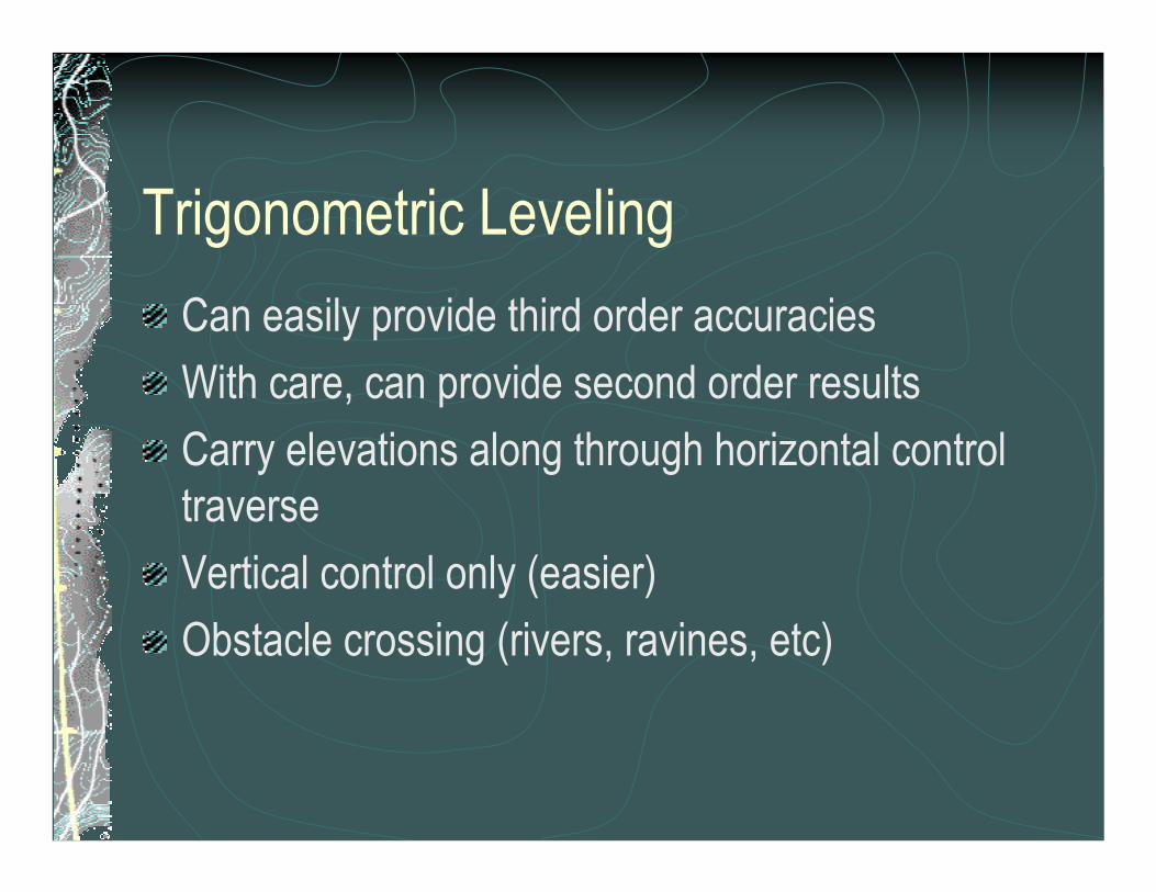
Trigonometric LevelingCan easily provide third order accuraciesWith care, can provide second order resultsCarry elevations along through horizontal control traverseVertical control only (easier)Obstacle crossing (rivers, ravines, etc)

TraverseMust keep sight distances shorter than would normally be done in a traverseUse forced centering OR carefully measure HI’s and HT’s (potential error source!)Should always measure distances and vertical angles forward and back, not just one way

Pure Trig levelsHorizontal not importantLeapfrog ahead similar to conventional differential leveling, no need to record HIUse fixed height pole, no need to record HT’s, simplifies computationsGreater productivity in hilly areasLIMIT SIGHT DISTANCE!

Trigonometric HeightingObservations are affected by deflection of the verticalObservations are affected by curvature and refractionWe need orthometric height differences, so ignore deflections (for short distances)

Curvature and RefractionAL is level lineAH is tangent to surface at AHL is curvature correctionHP is refraction correctionPL is combined correction

Coefficient of RefractionRatio between the refraction angle and the angle at the center of the earthCan vary from –2.0 to +1.50 for grazing rays close to the groundUsually assume a value of k=0.13For σk of 1.0:
Error in height for 100 m sight: 0.8 mmError in height for 300 m sight: 7.0 mmError in height for 500 m sight: 19.6 mm

To determine k
Observe simultaneously from both ends“Near” simultaneous is more feasible
K=0.5+15.4728(θa+θb)/S
Where θa and θb are in seconds of arc, S is in meters

Curvature & Refraction
CR=S2(1-k)/2R
Where:k is the coefficient of refraction (0.13?)R is the radius of the earthS is the distance measured

Conventional LevelingCurvature and refraction cancel out for short sightsHorizontal line of sight Limits sighting distance in hilly areas

One way zenith distance

One way zenith distance
Uncertainty in k, refraction coefficient, is the limiting factor for this method
•H2 -H1=d * cos Z + (1-k)*(d * sin Z)2 /2*R

Reciprocal Zenith Distances
Uncertainty in k can be greatly reduced if reciprocal, simultaneous zenith distances are observedUncertainty in σ∆k:
Error in height for 100 m sight: 0.1 mm (0.8)Error in height for 300 m sight: 1.0 mm (7.0)Error in height for 500 m sight: 2.9 mm (19.6)
H2-H 1=d*(cos Z12-cos Z21)/2

Trig HeightingAdd HI and subtract HR to get ∆H between monumentsMAJOR SOURCE of ERROREliminate by using leapfrog method or forced centering
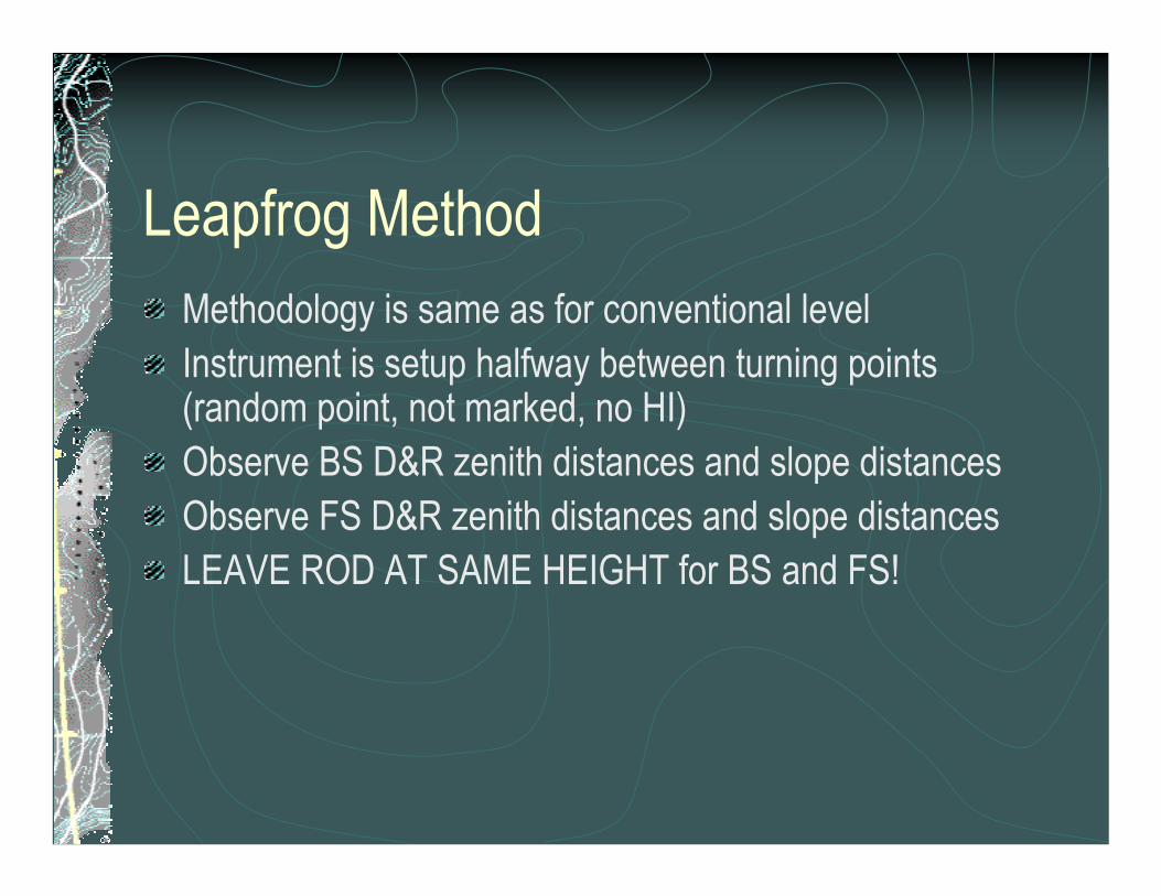
Leapfrog MethodMethodology is same as for conventional levelInstrument is setup halfway between turning points (random point, not marked, no HI)Observe BS D&R zenith distances and slope distancesObserve FS D&R zenith distances and slope distancesLEAVE ROD AT SAME HEIGHT for BS and FS!

Leapfrog MethodAlternatively, record only vertical distance for each sight, mean the D&RComputations greatly reducedIf BS distance≅FS distance, and ∆t is small, C & R will cancel

Obstacle CrossingSetup four tripods, two on each sideSet a TBM nearby (10-20 m)Setup a total station (preferably 1”) on one tripod on each side, and a target/prism on the other tripod on each sideCan be done with separate EDM/theodolite

Obstacle Crossing – Each SideObserve 4 D&R zenith distances to 4 different rod graduations on TBM (i.e. 1.00,2.00,3.00,4.00) Observe 2 D&R zenith distances and EDM distances to nearby target and opposite targetSecond order accuracy up to 500 m

Vertical ControlMethods of determining elevation differences.Vertical DatumsStandards and SpecificationsEquipmentSources of ErrorComputations and Adjustment of Level Data

Vertical Control
Differential Leveling

Differential Leveling

“Loop” Examples

Vertical DatumsNAVD 88NGVD 29Local datumsUSGS ≠NGS (NOS,USCGS)

Standards and Specifications
Standards and Specifications for Geodetic Control Networks, FGCC-1984Geospatial Positioning Accuracy Standards, FGDC, FGCS-1998Local standards (DOTs, etc)Draft of standards for digital levels
Orders and Classes of Accuracy
First OrderClass IClass II
Second OrderClass IClass II
Third Order

Maximum Closure Examples
1st OrderClass I (4mm*K1/2) (loop or line)
12.6 mm in 10 km (0.041 ft in 6.2 miles)Class II (5mm*K1/2 ) (loop or line)
15.8 mm in 10 km (0.052 ft in 6.2 miles)

Maximum Closure Examples
2nd OrderClass I (6mm*K1/2)
19.0 mm in 10 km (0.062 ft in 6.2 miles)Class II (8mm*K1/2 ) (loop or line)
25.3 mm in 10 km (0.083 ft in 6.2 miles)

Maximum Closure Examples
3rd Order(12mm*K1/2) or (0.05ft*M1/2)
12.0 mm in 1.61 km (0.050 ft in 1 mile)34.0 mm in 8.1 km (0.112 ft in 5 miles)48.1mm in 16.1 km (0.158 ft in 10 miles)

Equipment for Direct LevelingLevels
DumpyTiltingAutomaticDigital
Rods (staffs)FiberglassWoodInvar
Tripods, Turning Points, Verniers, Struts, Rod Levels, etc.
Sources of Error in LevelingInstrument ErrorsParallaxEarth’s curvatureAtmospheric RefractionVariations in TemperatureRod errors (equipment not people)Human error

Typical Direct Leveling ProjectDefine Scope of Work
Determines Equipment and Methodology requiredResearch and Recover Existing ControlEstablish TBM’s and PBM’sPlan Primary and Secondary LoopsPerform Field OperationsReduce, Compute, and Adjust DataReport Results

Preparation for Field Work (Two Peg Test)
Makes line of sight parallel to the axis of the level tubeManual adjustment for most levels“Software” adjustment of some digital levels (doesn’t physically move crosshair)
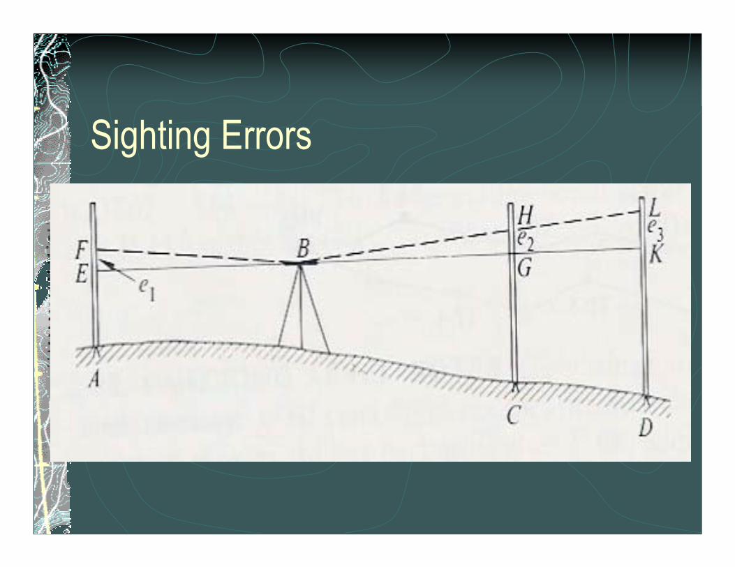
Sighting Errors

Two Peg Test
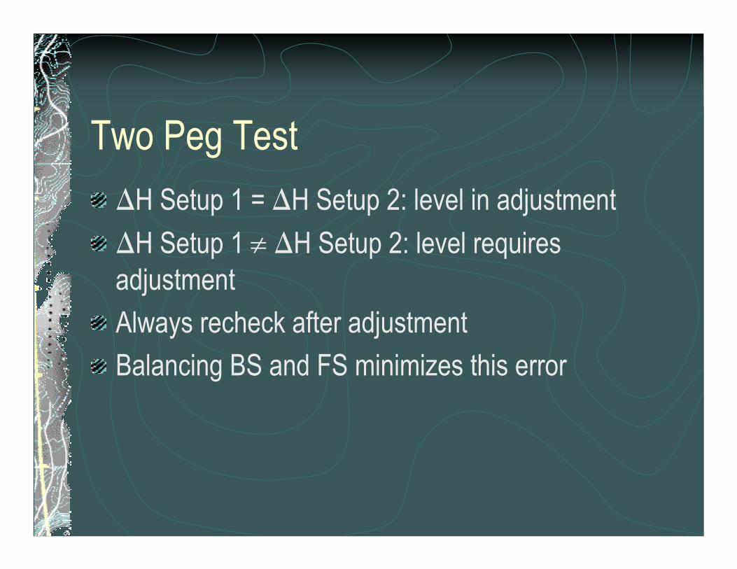
Two Peg Test∆H Setup 1 = ∆H Setup 2: level in adjustment∆H Setup 1 ≠ ∆H Setup 2: level requires adjustmentAlways recheck after adjustmentBalancing BS and FS minimizes this error

Alternative Two Peg Test MethodsForstner Method
Nahbauer Method
Kukkamaki Method

Three Wire LevelingAlso called “precise leveling”All three crosshairs (threads) read and recordedKnown thread spacing allows computation of interval distanceUse of digital level eliminates need for three wire leveling

Three Wire Level Notes
Collimation Correction(C factor)
C factor is used to correct for inclined line of sight when precise levels are run. ΣBS ≠ ΣFS.

C factorC = (Σ near rod readings - Σ far rod readings)
/ (Σ far rod intervals - Σ near rod intervals)
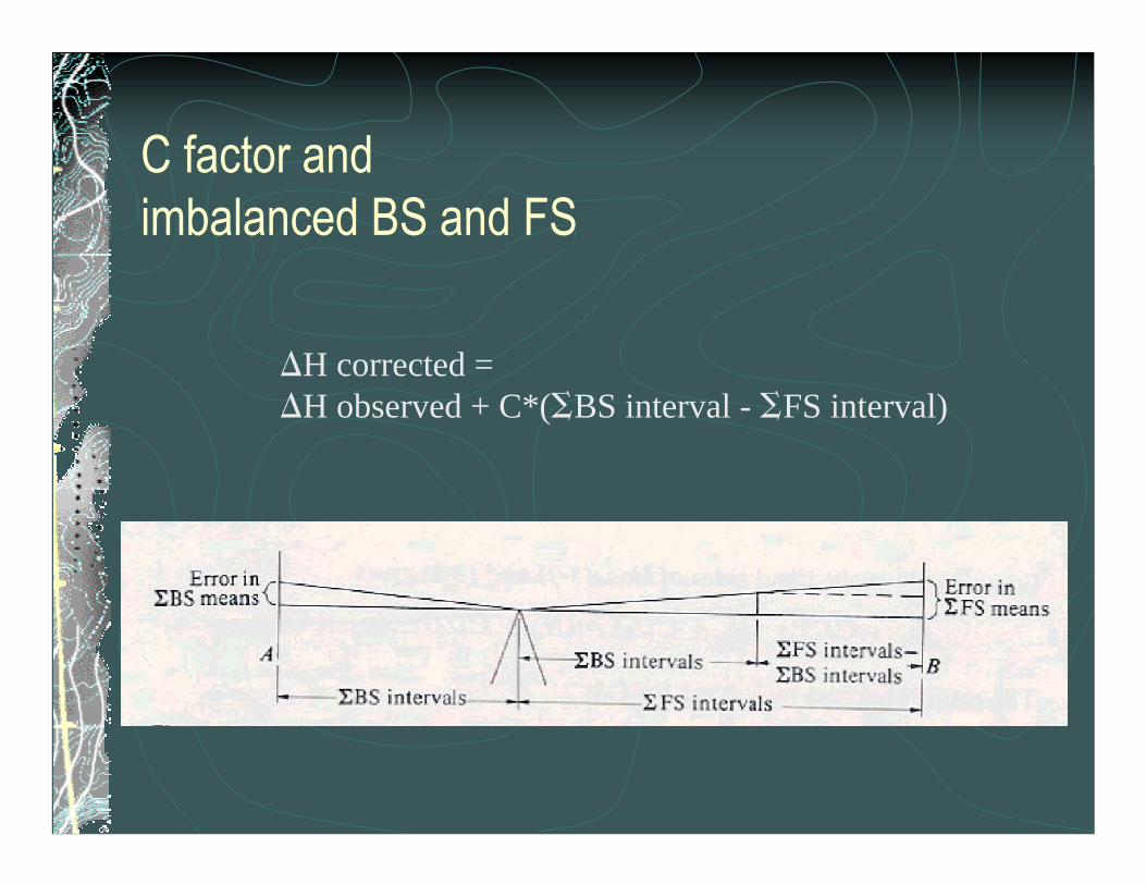
C factor and imbalanced BS and FS
∆H corrected = ∆H observed + C*(ΣBS interval - ΣFS interval)

Reciprocal LevelingUsed when leveling across large obstructionsRivers, Ravines, Canyons, Bridges

Reciprocal LevelingLevel set up on one side and readings taken on near and far rods, ∆H1 obtained.Procedure repeated for other side, ∆H2 obtained.Average of ∆H1 and ∆H2 computed.Multiple readings or using two levels increases accuracy of results.

ComputationsSingle line or loop of levels
Begin at known elevationEnd at known elevationMisclosure at end of runAdjust elevations of intermediate pointsCorrections made directly proportional to the number of setups or distances between points

Single Loop or Line ComputationsExample:
10 mile runMisclosure of +0.35 feet5 intermediate BM’s setElevations corrected by distanceElevations corrected by number of turns

Single loop example
Station Observed HDistancefrom BM Correction Adjusted H
Number of
turns Correction Adjusted H
Differencebetweenmethods
BM 470.680 0 0.000 470.680 0 0.000 470.680 0.000TBM1 479.350 1.7 -0.060 479.291 25 -0.044 479.306 -0.016TBM2 486.350 3 -0.105 486.245 45 -0.079 486.271 -0.026TBM3 460.280 5 -0.175 460.105 95 -0.166 460.114 -0.009TBM4 451.350 7.8 -0.273 451.077 130 -0.228 451.123 -0.046TBM5 480.020 9 -0.315 479.705 160 -0.280 479.740 -0.035BM 520.740 10 -0.350 520.390 200 -0.350 520.390 0.000
Adjusted H = Observed H + ((distance from BM / total distance) * misclosure)
Adjusted H = Observed H + ((turns from BM / total turns) * misclosure)

Multiple loop level runsBegin on known elevationEnd on known elevationMay have intermediate known elevationsMay run individual loops more than onceMay have several (many) interconnected loops

Multiple loop level runsHave more than one observed elevation for new BM’sGoal is to compute the best unique value for each new BMLeast Squares provides the best available solution

Why Least Squares??Uses weighted means to obtain a solution
Weights can be based on number of turns or distance of a run
Uses observed differences in elevation and observed elevations
This is what we measure in a level runComputer software readily available
Digital level files read directly by some softwareCheck for blundersEstimation of error

Least Squares Example

Least Squares ExampleMultiple elevations at B,C, and D from raw measurementsKnown elevations at A and FMeasured height differences and length of runs (could use number of turns)

Least Squares ExampleWeights
Use distance between pointsErrors in elevation difference varies with distance between pointsWeight for observations obs1= 1 / 2.01obs2=1 / 0.84, etc….
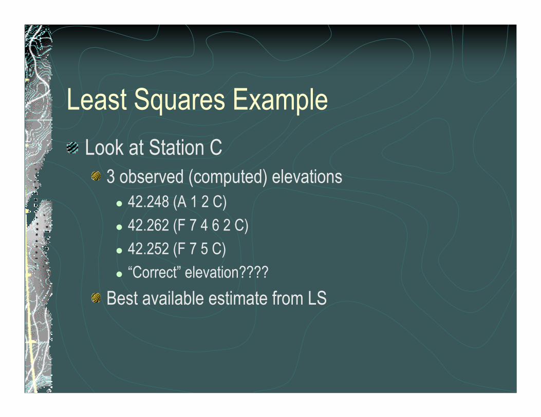
Least Squares ExampleLook at Station C
3 observed (computed) elevations42.248 (A 1 2 C)42.262 (F 7 4 6 2 C)42.252 (F 7 5 C)“Correct” elevation????
Best available estimate from LS

Least Squares Example3 elevations at C
distance oflevel line
42.248 2.8542.262 17.742.252 3.98
mean 42.254IS THIS OUR BEST ESTIMATE??? NO!!!
USE A WEIGHTED AVERAGE
C = 42.250
variance at C = 0.004 (from LS adjustment output)
42.248*(1/2.85) + 42.262*(1/17.7) + 42.252*(1/3.98)=(1/2.85)+(1/17.7)+(1/3.98)

Using Least SquaresCheck out various programs
TrainingExperienceConsultantsCompatibility with file types

Typical steps in a LS adjustment using a software package
Load the dataFix (hold) one known elevation and run adjustment
“Free” or minimally constrained adjustmentReview results: compare computed elevations at other known BM’s
Fix additional known BM’s and run subsequent adjustments