2007-8-13 KDD 2007, San Jose

Fast Direction-Aware Proximity for Graph Mining

Speaker: Hanghang Tong

Joint work w/ Yehuda Koren, Christos Faloutsos

2

Proximity on Graph

• Un-directed graph– What is Prox between A and B– ‘how close is Smith to Johnson’?

But, many real graphs are directed….

A B

1 1

1

111

1

3

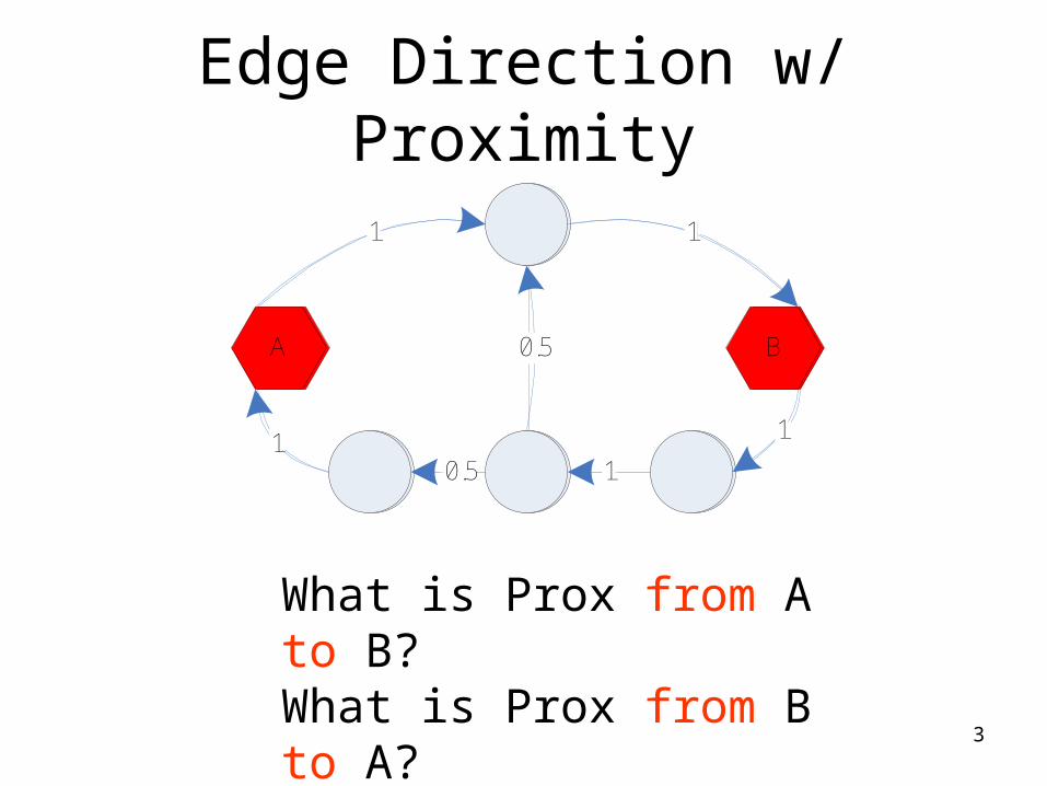
Edge Direction w/ Proximity

A B

1 1

1

111

1A B

1 1

1

10.51

0.5

What is Prox from A to B?What is Prox from B to A?

4

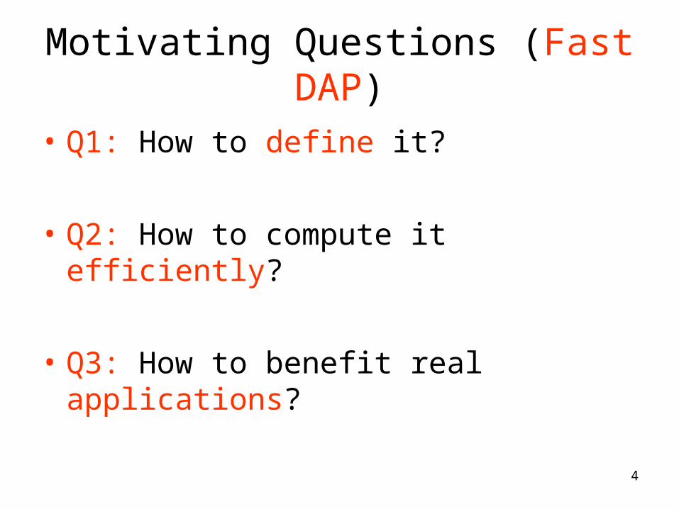
Motivating Questions (Fast DAP)

• Q1: How to define it?

• Q2: How to compute it efficiently?

• Q3: How to benefit real applications?

5

Roadmap

• DAP definitions– Escape Probability– Issue # 1: ‘degree-1 node’ effect– Issue # 2: weakly connected pair

• Computational Issues– FastAllDAP: ALL pairs– FastOneDAP: One pair

• Experimental Results• Conclusion

6

Defining DAP: escape probability

• Define Random Walk (RW) on the graph• Esc_Prob(AB)

– Prob (starting at A, reaches B before returning to A)

Esc_Prob = Pr (smile before cry)

A Bthe remaining graph

7

Esc_Prob: Example

Esc_Prob(a->b)=1 > Esc_Prob(b->a)=0.5

A B

1 1

1

10.51

0.5

8

Esc_Prob is good, but…

• Issue #1: – `Degree-1 node’ effect

• Issue #2:– Weakly connected pair

Need some practical modifications!

9

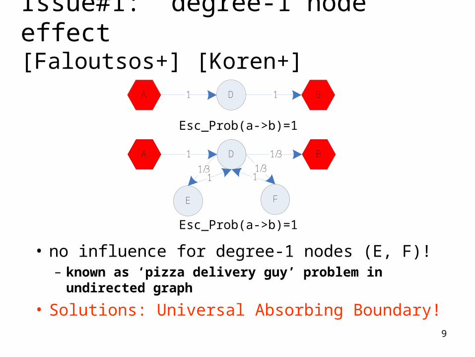
Issue#1: `degree-1 node’ effect[Faloutsos+] [Koren+]

• no influence for degree-1 nodes (E, F)!– known as ‘pizza delivery guy’ problem in

undirected graph

• Solutions: Universal Absorbing Boundary!

A BD1 1

A BD1 1/3

E F

1/31/311

Esc_Prob(a->b)=1

Esc_Prob(a->b)=1

10

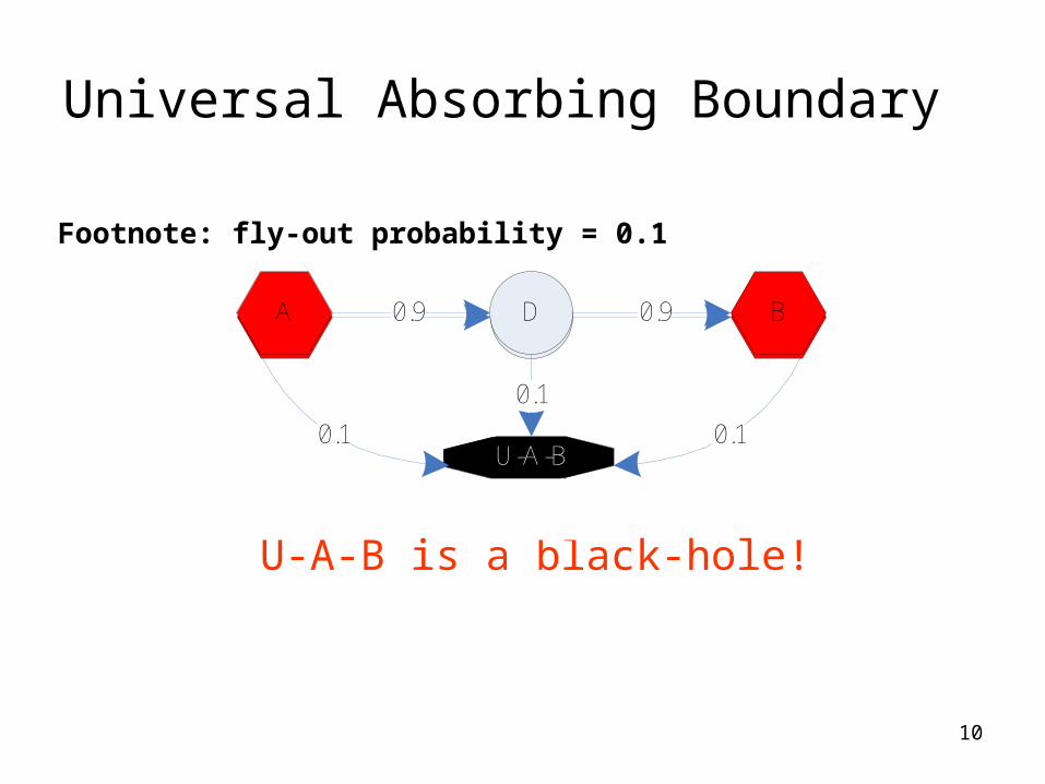
Universal Absorbing Boundary

U-A-B is a black-hole!

A BD1 1

U-A-B

Footnote: fly-out probability = 0.1

A BD0.9 0.9

U-A-B0.1

0.1

0.1

1

11

Introducing Universal-Absorbing-Boundary

A BD0.9 0.9

U-A-B0.1

0.1

0.1

A BD0.9 0.3

E F

0.30.30.90.9

U-A-B

0.1

0.10.10.10.1

Prox(a->b)=0.91

Prox(a->b)=0.74

A BD1 1

A BD1 1/3

E F

1/31/311

Footnote: fly-out probability = 0.1

Esc_Prob(a->b)=1

Esc_Prob(a->b)=1

12

Issue#2: Weakly connected pair

A B1 1 1

wi j

Prox(AB) = Prox (BA)=0

Solution: Partial symmetry!

a w

i j

(1-a) w

.

.

13

Practical Modifications: Partial Symmetry

A B1 1 1

Prox(AB) = Prox (BA)=0

A B0.9 0.9 0.9

0.1 0.1 0.1

Prox(AB) =0.081 > Prox (BA)=0.009

14

Roadmap

• DAP definitions– Escape Probability– Issue # 1: ‘degree-1 node’ effect– Issue # 2: weakly connected pair

• Computational Issues– FastAllDAP: ALL pairs– FastOneDAP: One pair

• Experimental Results• Conclusion

15

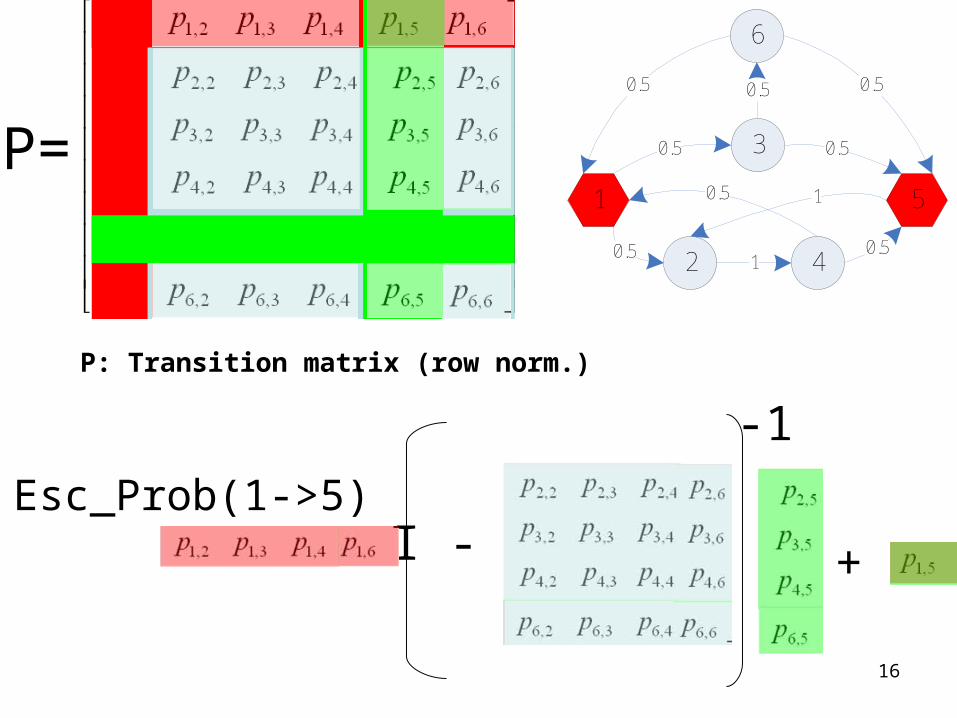
Solving Esc_Prob: [Doyle+]

P: transition matrix (row norm.)n: # of nodes in the graph

1 x (n-2) 1 x (n-2)(n-2) x (n-2)

One matrix inversion , one Esc_Prob!

i^th row removing i^th & j^th elements

P removing i^th & j^th rows & cols

i^th col removing i^th & j^th elements

16

Esc_Prob(1->5) =

1,1 1,2 1,3 1,4 1,5 1,6

2,1 2,2 2,3 2,4 2,5 2,6

3,1 3,2 3,3 3,4 3,5 3,6

4,1 4,2 4,3 4,4 4,5 4,6

5,1 5,2 5,3 5,4 5,5 5,6

6,1 6,2 6,3 6,4 6,5 6,6

p p p p p p

p p p p p p

p p p p p p

p p p p p p

p p p p p p

p p p p p p

P=

I - +

-1

1 5

3

2

6

4

0.5 0.5

0.5

0.50.5

0.5

0.5

1

0.5 1

P: Transition matrix (row norm.)

17

Solving DAP (Straight-forward way)

One matrix inversion, one proximity!

2 1,

ˆProx( )=c ( )ti j i ji j p I cP p c p

1 x (n-2) 1 x (n-2)(n-2) x (n-2)

1-c: fly-out probability (to black-hole)

18

• Case 1, Medium Size Graph– Matrix inversion is feasible, but…– What if we want many proximities?– Q: How to get all (n ) proximities efficiently?– A: FastAllDAP!

• Case 2: Large Size Graph – Matrix inversion is infeasible– Q: How to get one proximity efficiently?– A: FastOneDAP!

Challenges

2

19

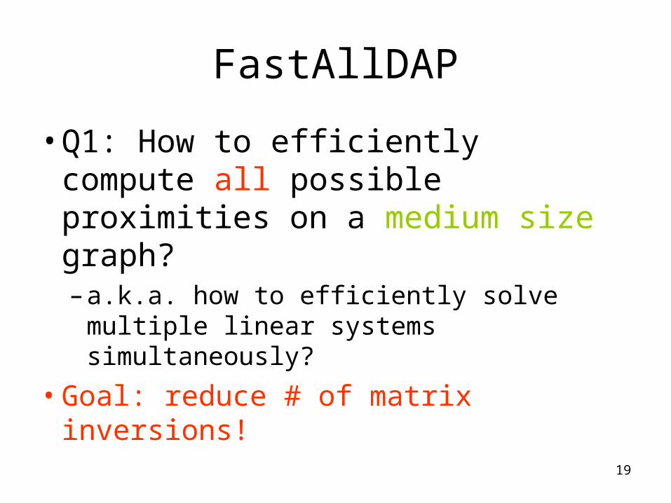
FastAllDAP

• Q1: How to efficiently compute all possible proximities on a medium size graph?– a.k.a. how to efficiently solve multiple

linear systems simultaneously?

• Goal: reduce # of matrix inversions!

20

1,1 1,2 1,3 1,4 1,5 1,6

2,1 2,2 2,3 2,4 2,5 2,6

3,1 3,2 3,3 3,4 3,5 3,6

4,1 4,2 4,3 4,4 4,5 4,6

5,1 5,2 5,3 5,4 5,5 5,6

6,1 6,2 6,3 6,4 6,5 6,6

p p p p p p

p p p p p p

p p p p p p

p p p p p p

p p p p p p

p p p p p p

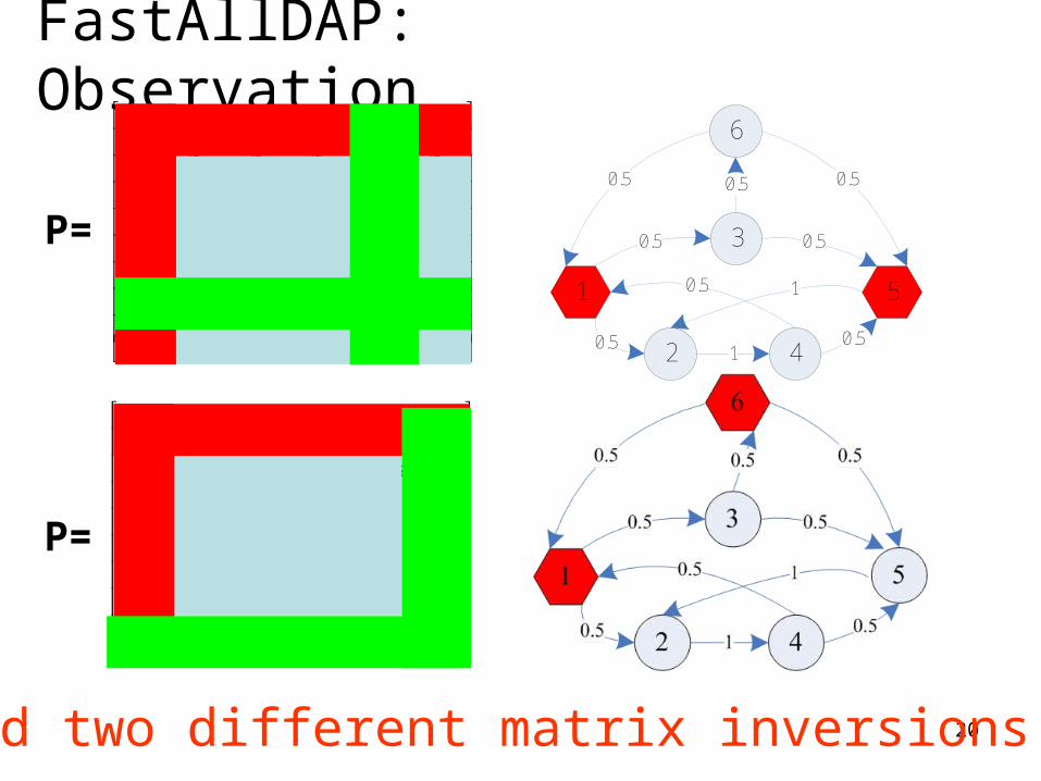
FastAllDAP: Observation

1 5

3

2

6

4

0.5 0.5

0.5

0.50.5

0.5

0.5

1

0.5 1

1,1 1,2 1,3 1,4 1,5 1,6

2,1 2,2 2,3 2,4 2,5 2,6

3,1 3,2 3,3 3,4 3,5 3,6

4,1 4,2 4,3 4,4 4,5 4,6

5,1 5,2 5,3 5,4 5,5 5,6

6,1 6,2 6,3 6,4 6,5 6,6

p p p p p p

p p p p p p

p p p p p p

p p p p p p

p p p p p p

p p p p p p

Need two different matrix inversions!

P=

P=

21

1,1 1,2 1,3 1,4 1,5 1,6

2,1 2,2 2,3 2,4 2,5 2,6

3,1 3,2 3,3 3,4 3,5 3,6

4,1 4,2 4,3 4,4 4,5 4,6

5,1 5,2 5,3 5,4 5,5 5,6

6,1 6,2 6,3 6,4 6,5 6,6

p p p p p p

p p p p p p

p p p p p p

p p p p p p

p p p p p p

p p p p p p

FastAllDAP: Rescue

1,1 1,2 1,3 1,4 1,5 1,6

2,1 2,2 2,3 2,4 2,5 2,6

3,1 3,2 3,3 3,4 3,5 3,6

4,1 4,2 4,3 4,4 4,5 4,6

5,1 5,2 5,3 5,4 5,5 5,6

6,1 6,2 6,3 6,4 6,5 6,6

p p p p p p

p p p p p p

p p p p p p

p p p p p p

p p p p p p

p p p p p p

Redundancy among different linear systems!

P=

P=

Overlap between two gray parts!

Prox(1 5)

Prox(1 6)

22

FastAllDAP: Theorem

• Theorem:

• Proof: by SM Lemma

• Example:

23

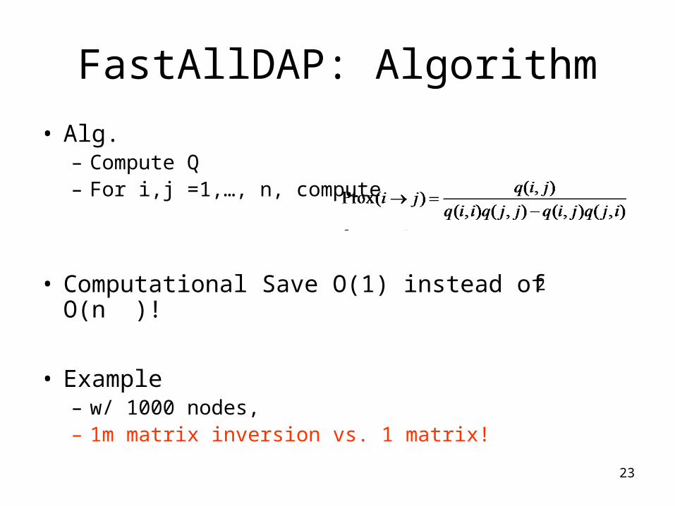
FastAllDAP: Algorithm

• Alg.– Compute Q– For i,j =1,…, n, compute

• Computational Save O(1) instead of O(n )!

• Example– w/ 1000 nodes, – 1m matrix inversion vs. 1 matrix!

2

24

FastOneDAP

• Q1: How to efficiently compute one single proximity on a large size graph?– a.k.a. how to solve one linear system

efficiently?

• Goal: avoid matrix inversion!

25

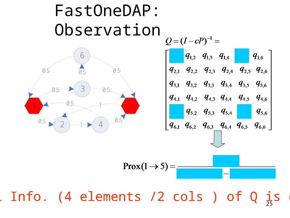
FastOneDAP: Observation

1 5

3

2

6

4

0.5 0.5

0.5

0.50.5

0.5

0.5

1

0.5 1

Partial Info. (4 elements /2 cols ) of Q is enough!

26

FastOneDAP: Observation

• Q: How to compute one column of Q?• A: Taylor expansion

Reminder:

i col of Qth

[0, …0, 1, 0, …, 0]T

27

FastOneDAP: Observation

x x x

Sparse matrix-vector multiplications!

….

i col of Qth

[0, …0, 1, 0, …, 0]T

28

FastOneDAP: Iterative Alg.

• Alg. to estimate i Col of Qth

29

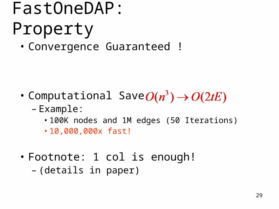
FastOneDAP: Property

• Convergence Guaranteed !

• Computational Save– Example:

• 100K nodes and 1M edges (50 Iterations)• 10,000,000x fast!

• Footnote: 1 col is enough! – (details in paper)

30

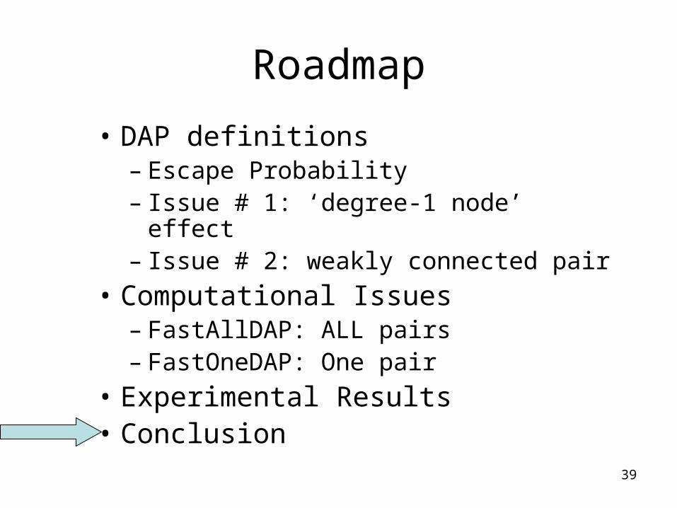
Roadmap

• DAP definitions– Escape Probability– Issue # 1: ‘degree-1 node’ effect– Issue # 2: weakly connected pair

• Computational Issues– FastAllDAP: ALL pairs– FastOneDAP: One pair

• Experimental Results• Conclusion

31

Datasets (all real)

Name Node # Edge # Directionality

WL 4k 10k A-links to-B

PC 36k 64k Who-contact-whom

EP 76k 509k Who-trust-whom

CN 28k 353k A-cites-B

AE 38k 115k Who-email to-whom

330 0.01 0.02 0.03 0.04 0.05 0.06 0.07 0.08 0.09

0

0.05

0.1

0.15

0.2

0.25

0 0.01 0.02 0.03 0.04 0.05 0.06 0.07 0.08 0.090

0.02

0.04

0.06

0.08

0.1

0.12

0.14

0.16

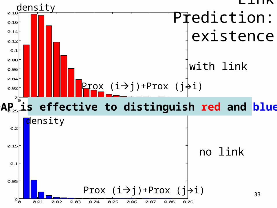
0.18 Link Prediction: existence

no link

with link

density

density

Prox (ij)+Prox (ji)

Prox (ij)+Prox (ji)

DAP is effective to distinguish red and blue!

35

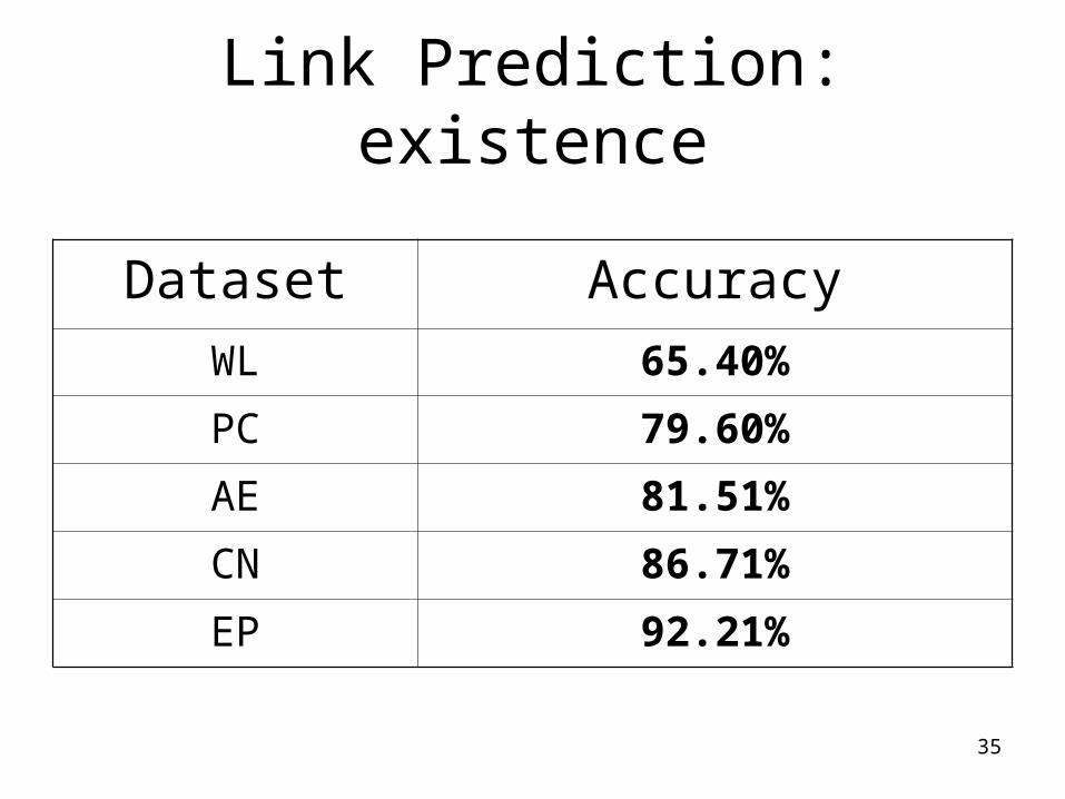
Link Prediction: existence

Dataset Accuracy

WL 65.40%

PC 79.60%

AE 81.51%

CN 86.71%

EP 92.21%

36

Link Prediction: direction

• Q: Given the existence of the link, what is the direction of the link?

• A: Compare prox(ij) and prox(ji)>70%

Prox (ij) - Prox (ji)

density

37

Efficiency: FastAllDAP

Size of Graph

Time (sec)

Straight-Solver

FastAllDAP

1,000xfaster!

38

Efficiency: FastOneDAP

Size of Graph

Time (sec)

FastOneDAP

Straight-Solver

1,0000xfaster!

39

Roadmap

• DAP definitions– Escape Probability– Issue # 1: ‘degree-1 node’ effect– Issue # 2: weakly connected pair

• Computational Issues– FastAllDAP: ALL pairs– FastOneDAP: One pair

• Experimental Results• Conclusion

40

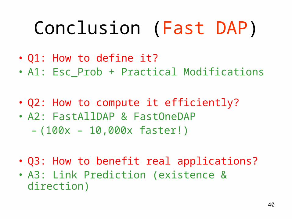
Conclusion (Fast DAP)

• Q1: How to define it?• A1: Esc_Prob + Practical Modifications

• Q2: How to compute it efficiently?• A2: FastAllDAP & FastOneDAP

– (100x – 10,000x faster!)

• Q3: How to benefit real applications?• A3: Link Prediction (existence & direction)

41

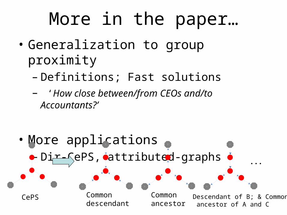
More in the paper…• Generalization to group proximity

– Definitions; Fast solutions– ‘How close between/from CEOs and/to

Accountants?’

• More applications– Dir-CePS, attributed-graphs

A C

B

A C

B

A C

B

A C

B

CePS Common descendant

Common ancestor

Descendant of B; & Common ancestor of A and C

...

42

Cupid uses arrows, so does graph mining!

Thank you!www.cs.cmu.edu/~htong

43

Back-up foils

44

DAP: Size Bias [Koren+]

We want:

A B

Candidate Graph

Original Graph

Prox ( ) Prox ( )candi origianla b a b

Prox ( ) Prox ( )candi origianla b a b

Solution: degree preserving!

Actually:

45

Practical Modifications: Degree-Preserving

A B

D

E

G

F

0.5 0.5

1

0.50.5

0.5

0.5

1

A B

D

E F

0.5 1

10.51

A B

D

E F

0.5 0.5

1

0.5

0.51

G

A->D->B

A->E->F->B

A->D->G->B

Original graph: Prox(a->b)=0.875

Prox(a->b)=1

Prox(a->b)=0.75Paths (A->B):

46

Practical Modifications: Degree-Preserving

1 1.5 2 2.5 3 3.5 4 4.5 5 5.5 60.097

0.0975

0.098

0.0985

0.099

0.0995

0.1

0.1005

0.101

Size (# of Hop)

Mea

n E

scap

e P

rob

Evaluate on Size Bias

with degree preservation

without degree preservation

Size of Graph

Proximity

47

Solving DAP: [Doyle+]• Key quantity:

– Pr (RW starting at k, will visit j before i)–

1 5

3

2

6

4

0.5 0.5

0.5

0.50.5

0.5

0.5

1

0.5 1

( , )kv j i

,Prox( ) ( , )i k kki j p v j i

1 2 3

4 5 6

Prox( ) 0 (5,1) 0.5 (5,1) 0.5 (5,1)

0 (5,1) 0 (5,1) 0 (5,1) 0.625

i j v v v

v v v

1 2

3 4

5 6

(5,1) 0 (5,1) 0.5

(5,1) 0.75 (5,1) 0.5

(5,1) 1 (5,1) 0.5

v v

v v

v v

Q: How to solve ?

( , )kv j i

48

• Setup a linear system

2 1 3 4 5 6

3 1 2

2,1 2,3 2,4 2,5 2,6

3,1 3,2 3,4 3,5 3,6

4,1 4,2 4,3 4,5 4,6

5,1 5,2 5,3 5,4 6,5

1 1 2 2 3

4 5 6

4 1 2 3 5 6

6 1 2 3 4 5

5

1

0

1

(5,1), (5,1),

x x x x x x

x x x x x x

x x x

p p p p p

p p p p p

p p p p p

p p p p p

x v

x x x

x x x x

x

x

x

x

x

x

v

3

4 4 5 5 6 6

(5,1),

(5,1), (5,1), (5,1)

v

x v x v x v

Solving [Doyle+]( , )kv j i

Harmonicproperty

Boundary condition

1 5

3

2

6

4

0.5 0.5

0.5

0.50.5

0.5

0.5

1

0.5 1

49

Effectiveness: CePS

A C

B

A C

B

Original GraphBlack: query nodes

CePS

50

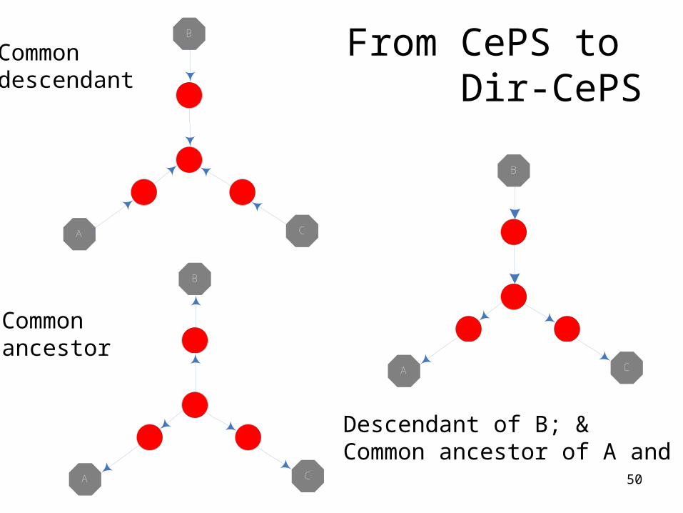
From CePS to Dir-CePS

A C

B

A C

B

Common descendant

Common ancestor

A C

B

Descendant of B; &Common ancestor of A and C