2010:078 master's thesis development of an efficient ...1023156/fulltext01.pdf · 2010:078...

2010:078

M A S T E R ' S T H E S I S

Development of an Efficient AnalysisMethod for Prediction and StructuralDimensioning of Space Structures

Subjected to Shock Loading

Nadeem Siam

Luleå University of Technology

Master Thesis, Continuation Courses Space Science and Technology

Department of Space Science, Kiruna

2010:078 - ISSN: 1653-0187 - ISRN: LTU-PB-EX--10/078--SE

Nadeem SIAM

Development of an Efficient Analysis Method for Prediction and

Structural Dimensioning of Space Structures Subjected to Shock

Loading

Space AB

School of Engineering

Astronautics and Space Engineering

(SpaceMaster)

MSc Thesis Academic year: 2009-2010

Supervisors Magnus BAUNGE – RUAG Space AB

Tom DE VUYST – Cranfield University

Rade VIGNJEVIC – Cranfield University

July 2010

Nadeem SIAM Cranfield University RUAG Space AB

I

School of Engineering

Astronautics and Space Engineering

(SpaceMaster)

MSc Thesis Academic year: 2009-2010

Nadeem SIAM

Development of an Efficient Analysis Method for Prediction and

Structural Dimensioning of Space Structures Subjected to Shock

Loading

RUAG Space AB

Supervisors Magnus BAUNGE – RUAG Space AB

Tom DE VUYST – Cranfield University

Rade VIGNJEVIC – Cranfield University

July 2010

This thesis is submitted in partial fulfillment of the requirements for the degree of

Master of Science.

© Cranfield University 2010. All rights reserved. No part of this publication may be

reproduced without the written permission of the copyright owner.


III

ABSTRACT

Space structures face many different and extreme types of loading throughout their

life time from harsh launch environment to the harsh space environment. Dynamic

loading in space structures is found to be the main concern with its variety and

extreme loading conditions from periodic loading to acoustic/random vibration and

shocks. Shock in space structures are produced by pyrotechnic devices placed in the

launchers initiating the stage separations, in addition, other less intense shock sources

can be the deployment mechanisms for solar cells, antennas, and other satellite

components. These high intensity shocks are of a main concern for sensitive space

structures, like PCBs, crystals, and fragile optical components. Testing used to be the

main method for studying the effect of shocks on structures and components. But with

the increasing shock intensity in launchers due to the decreased amount of damping

materials, and the increasing customer qualification requirements, the possibility of

simulating shocks using Finite Element Models (FEM) has been studied. Different

possible simulations methods have been studied, applied to a simple model, and

compared with the ringing plate test results developing an efficient and reliable

method for shock simulation using Finite Element Methods. The effects of the

different parameter on the simulation results have been studied and some

recommendations for shock simulation using Finite Element Methods have been

conducted. The developed method have been studied further and applied to a more

complex real life model to study its effectiveness in simulating real space structures.

The overall outcome of the simulation method has proven its reliability in simulating

satellite structures subjected to Pyro-shocks and other shock loading when compared

to ringing plate test results. This simulation method has been developed at RUAG

Space AB in Göteborg, Sweden and has been approved as a possible simulation

method in their future shock analysis.

Key Words: Shocks, Shock Response Spectrum, SRS, Pyro-Shocks, Shock Simulation,

Finite Element Methods (FEM), Shock Testing, Dynamic Load Analysis, Pyro-technic

Devices, Space Structures, Transient Response Analysis.


V

ACKNOWLEDGMENT

I would like to dedicate this thesis to my parents who have always encouraged my

creativity and motivated me for my studies and the development of my knowledge, and

to my sister who always helped me through my hard decisions and hard time with her

confidence in me and her continues support. I will never forget when I was confused

about choosing the right field for my master studies and continuing in the field of Space

when she responded when I asked her about her opinion, she said “isn’t space your

childhood dream? Just go for it!” reminding me with my real childhood dream and

giving me the willingness and the spirit to advance and finish my studies successfully.

I would like to give a special thank to my supervisor Magnus Baunge at RUAG

Space AB for giving me the opportunity to work on this thesis topic and for his

continues support throughout my time at RUAG Space in Göteborg, Sweden. In

addition, I would also like to thank Jonas Leijon for his help with all the testing, and

everybody in the Mechanical Design Department for the nice time and for the really

interesting conversations even though they had to switch to English sometimes just for

me being around.

I would also like to thank my supervisors at Cranfield University Tom De Voyst and

Rade Vignjevic from the Applied Mechanics Department for their continuous support

and for their guidance throughout my thesis work.

Finally, I would also like to thank all my friends and everybody who supported me

in my studies and helped me throughout this course. I would like to dedicate a special

thanks to Cranfield ASE course coordinators, Peter Roberts, Steve Hobs, Jenifer, and

Debbie Coats for their support throughout my last year at Cranfield university. And also

a special thanks to the SpaceMaster Consortium and specially Sven Molin, Victoria

Barabash, and Anette Snällfot-Brändström for giving the opportunity to be part of this

course.

Thank you everybody!!


VI

TABLE OF CONTENTS

ABSTRACT ........................................................................................................................................ III ACKNOWLEDGMENT ....................................................................................................................... V TABLE OF CONTENTS .................................................................................................................... VI LIST OF FIGURES ........................................................................................................................... VII LIST OF TABLES .............................................................................................................................. IX ABBREVIATIONS ............................................................................................................................... X NOMENCLATURE ............................................................................................................................ XI

1. INTRODUCTION ............................................................................................................................. 1

1.1 MAIN AIM AND OBJECTIVES ........................................................................................................ 3 1.2 LITERATURE REVIEW ................................................................................................................... 3 1.3 LIMITATIONS ............................................................................................................................... 3

2. UNDERSTANDING SHOCKS ........................................................................................................ 5

2.1 PYRO-SHOCKS ............................................................................................................................. 5 2.2 SHOCK RESPONSE SPECTRUM (SRS) ........................................................................................... 8 2.3 SHOCK TESTING ........................................................................................................................... 9

2.3.1 Ringing Plate ........................................................................................................................ 10

3. SHOCK SIMULATION .................................................................................................................. 11

3.1 POSSIBLE SIMULATION METHODS USING FEM ......................................................................... 11 3.1.1 Modal Analysis ..................................................................................................................... 12 3.1.2 Frequency Response Analysis ............................................................................................... 13 3.1.3 Transient Response Analysis ................................................................................................ 14 3.1.4 NASTRAN’s SRS Method ...................................................................................................... 14

3.2 POSSIBLE EXCITATION METHODS .............................................................................................. 16

4. SIMPLE MODEL ............................................................................................................................ 21

4.1 BRACKET MODEL ...................................................................................................................... 21 4.2 RINGING PLATE TEST ................................................................................................................ 21 4.3 SIMULATION AND RESULTS COMPARISON ................................................................................. 24

5. EXPLANATION OF CHOSEN METHOD .................................................................................. 33

5.1 TRANSIENT RESPONSE .BDF FILE & SRS OUTPUT REQUEST ...................................................... 34 5.2 CONSTRAINTS AND EXCITATIONS .............................................................................................. 36 5.3 EFFECT OF DAMPING ................................................................................................................. 36 5.4 ELEMENT TYPE AND SIZE .......................................................................................................... 38

6. REAL LIFE MODEL ...................................................................................................................... 43

6.1 KU-BAND CONVERTER MODEL................................................................................................. 43 6.2 RINGING PLATE TEST ................................................................................................................ 44 6.3 SIMULATION AND RESULTS COMPARISON ................................................................................. 45

7. FURTHER WORK .......................................................................................................................... 49

8. CONCLUSION ................................................................................................................................ 51

9. REFERENCES ................................................................................................................................ 52

10. BIBLIOGRAPHY ....................................................................................................................... 53

11. APPENDIX ................................................................................................................................... A

11.1 APPENDIX A – SIMPLE MODEL TRANSIENT RESPONSE BDF FILE ................................................ A 11.2 APPENDIX B – SIMPLE MODEL NRL METHOD BDF FILE ............................................................. D 11.3 APPENDIX C – CONVERTER TRANSIENT RESPONSE BDF FILE ...................................................... F


VII

LIST OF FIGURES

Figure 1: The different shock events are separated in two different categories: shocks during

service life and shocks related to testing. ...................................................................................... 1

Figure 2: Artistic Imagination of Arian 5 Stages Separation - Courtesy of ESA. ......................... 2

Figure 3: GPS satellite with solar cells, antennas, and booms deployed. ..................................... 2

Figure 4: Typical time history of spacecraft pyrotechnic shock and its equivalent SRS [4]. ....... 5

Figure 5: Shock response spectrum and acceleration time-history for a near-field pyroshock.

The shock response spectrum is calculated from the inset acceleration time history using a 5

percent damping ratio. ................................................................................................................... 6

Figure 6: A typical shock response spectrum and acceleration time-history for a far field

pyroshock. The shock response spectrum is calculated from the inset acceleration time history

using a 5 percent damping ratio. The straight lines indicate tolerance bands (typically ±6 dB as

shown) which might be applied for qualification test specification. ............................................. 7

Figure 7: Array of single degree of freedom systems. .................................................................. 8

Figure 8: A common far-field qualification requirement SRS with its matching reproduced SRS

laboratory. ..................................................................................................................................... 9

Figure 9: Left: Ringing plate Diagram showing the pendulum mass, the guided tube and the

plate placed over a foam layer. Right: Ringing plate used at RUAG Space AB......................... 10

Figure 10: Test measured SRS in all translation directions (x, y, and z). ................................... 18

Figure 11: A simple tooth shaped pulse used to excite the rectangular shaped plate shown on the

right. ............................................................................................................................................ 19

Figure 12: Reproduced transient pulse. ....................................................................................... 19

Figure 13: Ringing plate with the simple structure fixed and ready for testing. ......................... 22

Figure 14: Simple model fixed on the ringing plate ready for testing......................................... 22

Figure 15: Test acceleration-time history measured at the bracket interface in the excitation

direction (y-direction). ................................................................................................................ 22

Figure 16: Test measured SRS at the bracket interface in X, Y, and Z-Directions vs.

qualification requirement SRS with its allowed tolerance level. ................................................ 23

Figure 17: Test measured SRS at the bracket interface vs. SRS measured at the top of the

bracket in excitation direction (Y-direction). .............................................................................. 23

Figure 18: Bracket meshed and constrained................................................................................ 24

Figure 19: Simulation predictions - input RED / output BLUE. ................................................. 25

Figure 20: Simulation acceleration-time history predictions compared to test measurements at

the bracket’s top sensor. .............................................................................................................. 26

Figure 21: Comparison between the Transient Response and the Frequency response compared

to the test results in Y-Direction. ................................................................................................ 27

Figure 22: Effect of SRS damping on calculated response spectrum. ........................................ 27

Figure 23: Frequency response stresses for 3 elements at the bent part on the top vs. static load

for the same elements on the bottom – both showing highly overestimated stress of about 400

MPa. ............................................................................................................................................ 28


VIII

Figure 24: Transient Response Stresses in 3 elements at the bend (Maximum about 69 MPa) –

bottom image zoomed. ................................................................................................................ 29

Figure 25: Recommended shock simulation procedure. ............................................................. 33

Figure 26: Effect of Different Types of Damping on the Output SRS using Transient Response

Analysis (top) – variable damping value used (bottom). ............................................................ 37

Figure 27: Bracket meshed with different element sizes. ........................................................... 39

Figure 28: Effect on element size on the simulation results for the Bracket. .............................. 40

Figure 29: 3D elements (tet10) vs. shell elements. ..................................................................... 40

Figure 30: Simulation results compared to test results after adjusting the element type, size, and

damping. ...................................................................................................................................... 41

Figure 31: Converter CAD model showing sensitive crystal and measurement location. .......... 43

Figure 32: Shaker test setup for the original PCB modes search on the left – the modified

mockup PCB on the right with the crystal replaced with an accelerometer. ............................... 43

Figure 33: Shock test set-up in Y, X, and Z-directions respectively. .......................................... 44

Figure 34: Converter’s near field qualification requirement with the matching reproduced SRS

using the ringing plate. ................................................................................................................ 44

Figure 35: KU-Band Converter Finite Element Model. .............................................................. 45

Figure 36: First three PCB mode shapes. .................................................................................... 46

Figure 37: Test results vs. simulation predictions in the Y-direction. ......................................... 47

Figure 38: Test results vs. simulation predictions in the X-direction. ......................................... 48

Figure 39: Test results vs. simulation predictions in the Z-direction. ......................................... 48


IX

LIST OF TABLES

Table 1: Bracket’s first ten normal modes. ................................................................................. 25

Table 2: Acceleration and stress levels using the NRL method. ................................................. 29

Table 3: Stress results using the NRL method with qualification SRS excitation in Y-direction.

..................................................................................................................................................... 30

Table 4: Stress results using the NRL method with test measured SRS in X, Y, and Z-directions.

..................................................................................................................................................... 31

Table 5: Stress Results using the ABS with Qualification SRS Excitation in Y-Direction. ....... 31

Table 6: Transient response required bulk data entry for SRS analysis [11]. ............................. 34

Table 7: PCB first mode compared to test measured mode using laser measurement and

accelerometer placed in the crystal location. ............................................................................... 45

Table 8: Converter’s first fifteen normal modes. ........................................................................ 46

Table 9: PCB’s first ten modes. .................................................................................................. 46


X

ABBREVIATIONS

Abbreviation Meaning

AD Applicable Document

ICDU Integrated Control and Data unit

ECSS European Cooperation for Space Standardization

ESA European Space Agency

FE Finite Element

FEA Finite Element Analysis

FEM Finite Element Models

FOS Factor of Safety

OBC On-Board Computer

PCB Printed Circuit Board

PROM Programmable Read-Only Unit

NASA National Aeronautics and Space Administration

NSGU Navigation Signal Generation Unit

NVM Non-Volatile Memory

RD Related Document

RSE RUAG Space AB

SCALE Sverker Christenson Advanced Light wEight

SMU Spacecraft Management Unit

SRS Shock Response Spectrum

TBC To Be Confirmed

TBD To Be Decided

TBW To Be Written

TCXO Temperature Controlled Crystal Unit

TRL Technology Readiness Level

TTRM Telemetry Telecommand Reconfiguration Mass Memory Module


XI

NOMENCLATURE

Notation Explanation

ωn Natural Frequency

ξ Critical Damping

λ Wave Length

E Modulus of Elasticity

ƒ Frequency

ρ Density

µ mass per surface area

π Pi ≈ 3.14

t Time

G Shear Modulus of Elasticity

C Wave Velocity

D bending stiffness

participation factors


1

1. INTRODUCTION

Space is the forefront of science and technology that we use in our daily lives in

communications, media, global positioning systems, weather forecasting, and new

science discoveries that helps us understand our universe and learn more about our

planet. Space structures face many different and extreme types of loading throughout

their life time from harsh launch environment to the harsh space environment. High

gravitational loads during launch, periodic vibrations, acoustic/random vibrations from

the launcher’s combustion chamber and high shock levels produced by pyro-technic

devices initiating stage separations, in addition to their weight limitations makes space

structures very demanding in their design process. Even after the rough launch stage,

satellites and space structures continue the rest of their lives in a rough space

environment subjected to vacuum, thermal stresses due to high temperature differences

in structures, debris, and radiations. In addition to this, maneuvering loads and

mechanisms deployment causes shock disturbances and shocks in most of space

structures. Space launch is the most expensive part of all space missions and its cost is

highly dependent on spacecraft size and weight. Therefore spacecrafts have to be strong

enough to withstand all the static and dynamic loads safely, yet have to be as light as

possible for the launch. These contradicting requirements make space structures very

challenging and demanding in their design and increase the need to avoid any

overdesigned structures for space applications.

Figure 1: The different shock events are separated in two different categories: shocks

during service life and shocks related to testing.

Dynamic loading is the main concern in spacecrafts with its variety and extreme

loading conditions from periodic loading to acoustic/random vibration and shocks.

Shocks are one of the most important types of load in a spacecraft, especially for brittle

structures and sensitive components. Pyro-shocks are the main and the most severe type

of shocks present in spacecrafts. They are produced by the pyro-technic devices placed

on bolts in the launcher initiating stage separations [1]. These shocks have very high

amplitude, in order of 1000 gs, and very high frequencies, exceeding 10000 Hz,

occurring for a very short period of time. This makes them very critical for sensitive

spacecraft structures and components [3], especially for electronic equipments (like

PCBs, electrical connections, relays, transformers, and sensitive crystals), structure

materials causing cracks and fractures in brittle materials (ceramics, crystals, epoxies or


2

glass envelopes), in addition to their impact on optical devices, mechanisms, and valves.

Other sources of shocks in spacecrafts can be due to the impulse loading of locking

devices in deployment mechanisms for solar cells, antennas, and optical devices in earth

observation missions [3]. Yet these other sources of shocks are not as intense as pyro-

shocks and have less impact on the spacecraft structures and its components.

Due to the complex nature of shocks and shock wave propagation in materials,

structures and sensitive spacecraft components are normally tested for shock loading

and are rarely simulated [2]. This is due to the limited capabilities that Finite Element

Methods (FEM) is known to have for high frequency simulation present in pyro-shock.

Testing is normally done at a later stage of the design process and can be expensive and

time consuming causing delays if modification is required at this late stage. With the

constant increase in shock levels in launchers due to the decreasing amount of damping

materials used in order to reduce weight, shocks and pyro-shocks are getting more

severe in Spacecrafts. In addition to the increasing customer qualification requirements

for shock, and with the advancement of computational methods, the development of an

efficient method for shock simulation using Finite Element Methods (FEM) is gaining

more importance. This results in a clear tendency today towards increasing shock levels

for satellite mounted equipment e.g. antennas and electronic units as developed by

RUAG Space AB. Therefore the need for an efficient simulation method with accurate

predictions to ensure sufficient dimensioning of equipment in order to avoid serious

failure during tests and launch is paramount. The possibility of shock simulation using

FEM is investigated further in the following sections. Many different simulation

methods are considered, compared, and applied to a simple structure as well as a more

complex and compact real space structure for the development of the most efficient

simulation method that can be used predict the effect of pyro-shocks and shock loading

in satellite components and space structures.

Figure 2: Artistic Imagination of Arian 5 Stages Separation - Courtesy of ESA.

Figure 3: GPS satellite with solar cells, antennas, and booms deployed.


3

1.1 Main Aim and Objectives

The main aim of this thesis work is the development of an efficient and reliable

analysis method for simulating structures under shock loading using Finite Element

Methods. This was done through the following objectives.

Material review and literature study.

Understanding shocks, shock testing, and shock qualification requirements.

Survey of applicable shock simulation methods.

Applications of MSC NASTRAN/PATRAN in similar analysis and

understanding their capabilities.

Applying different simulation methods to a simple model and comparing their

simulation predictions with test measurements.

Results comparison and discussion.

Selection of the most accurate and the most appropriate simulation method.

Studying the effect of the different parameters on the simulation predictions.

Defining the analysis procedure and guidelines.

Applying to a more complex real life problem (of interest to RUAG).

Final Presentation.

Documentation.

1.2 Literature Review

Many materials have been reviewed during this study. However, the available

material investigating shocks and shock simulation are limited. During the material

review most materials investigating shocks and shock testing mention that shocks can

only be tested due to the lack of shock simulation methods such as Neil T. Davie and

Vesta I. Bateman in Harris’ Shock and Vibration Handbook [3]. Yet some papers and

industrial studies investigating the possibilities of shock simulation using computational

methods, especially FEM, had other opinions ranging from possible such as M. de

Benedetti [6], possible with limited capabilities according to NASA’s Technical

Standards “Pyroshock Test Criteria” published May 18th

1999, and not possible such as

Neil T. Davie and Vesta I. Bateman in Harris’ Shock and Vibration Handbook [3] as

mentioned earlier. M.de Beneditti successfully simulated shocks using FEM using a

simple pulse equivalent to a certain qualification Shock Response Spectrum as will be

explained in more details in Chapter 3. This method was taken into account in our study

as well. However, other methods were proven more accurate and reliable providing

better predictions as will be explained in the following chapters. This confirms

possibility of shock simulation using finite element methods and increases the

confidence its simulation predictions as will be explained in more details in to following

chapters.

1.3 Limitations

The objective of this thesis work is to develop an efficient shock analysis method

that can be used for future shock analysis by RUAG Space AB in Göteborg, Sweden.

This is to be done with the available company resources and using the currently used

simulation software, MSC NASTRAN/PATRAN, available at the company. The


4

development of the simulation method is to be done by understanding shocks and the

available capabilities of the simulation software in order to make the most out of its

limited capabilities for the best simulation method, but no new simulation software is to

be developed.

The ringing plate available at RUAG Space AB is used for shock testing and to

validate and compare the simulation predications with test results. The availability of

the ringing plate for tests related to this study is however limited due to priorities given

to other ongoing projects. However any further testing that is expected to increase the

accuracy of simulation predictions compared to test measurements will be discussed in

the further study section.


5

2. UNDERSTANDING SHOCKS

Shocks are transient dynamic loads with very high frequencies (exceeding 10 KHz),

very high amplitudes (exceeding 1000 gs), and occurring for a very short period of time

(less than 20 milliseconds) which makes them different than other types of dynamic

loading. The high amplitude of shock loads by far exceeds any other type of dynamic or

static loading, but due to their very short duration they are considered a mild

environment and can rarely damage metallic structural members [2], however they are

very critical and are of main concern for sensitive space structures and components [2].

A shock is a normal transient pulse with a much shorter pulse duration compared to

the structures’ first natural period making it much faster than the structure response

causing the structure to continue vibrating freely and even reaching its peak response

after the shock pulse is over [5]. Pyro-shocks are the main and the most severe type of

shock loading present in space structures. Other types of shocks can be due to the

locking devices in deployment mechanisms of solar cells, antennas, and other pointing

devices. A typical pyroshock pulse has the shape of a high amplitude, exponentially

decaying multi-frequency sinusoid in a somehow symmetric manner around the zero

axis which is normally dampen out through the structure in less than 20 milliseconds as

can be seen on the left in Figure 4 [4].

Figure 4: Typical time history of spacecraft pyrotechnic shock and its equivalent SRS [4].

Due to the very short duration of shocks, they are normally measured as

acceleration-time history, which will be referred to here after as time history and as can

be seen on the left in Figure 4. Shock measurement in the form of a time-history is not

useful directly for engineering purposes as it lacks information about the frequency

contents of the shock, the maximum response of the structure where the shock is applied

and cannot be used for comparing similar shock pulses easily. Therefore the reduction

to a different form is then necessary. The Shock Response Spectrum (SRS) is found to

be a useful tool for shock representation and comparison used by engineers as can be

seen on the right in Figure 4 and as will be explained later in the following sections. [2]

2.1 Pyro-Shocks

Pyroshocks are the main and the most severe type of shock loading present in

launches and spacecrafts. As their name implies they are produced as a result from

firing pyrotechnic devices placed on bolts, nuts, pins, cutters, and other similar devices

in launchers during stage separations [1]. Pyrotechnic devices are explosive devices

used to cause failure to in certain locations in launchers initiating stage separation.


6

These explosive devices produce a nearly instantaneous pressure on surfaces with their

explosion producing high-frequency, high-amplitude stress waves travelling throughout

the structure. The energy in these high-frequency stress waves is gradually attenuated as

they travel through the structure due to material and structural damping and as they

travel through interface and connection points reaching nearly every point in the

launcher and its payload with different shapes and amplitude. The shape if the time-

history of these transient pulses depends on the pyrotechnic device used, the shape and

the properties of the structure, and the distance from the shock source. For this reason

space structures and components are divided into near-field and far-field components

depending on where and how far they will be placed away from the shock source and

therefore have to be designed according to the equivalent near- or far-field shock

qualification requirement accordingly. However, there is no fixed rule defining a

specific distance at which the near-field region ends and the far-field region starts and

they are normally classified according to some test techniques [3].

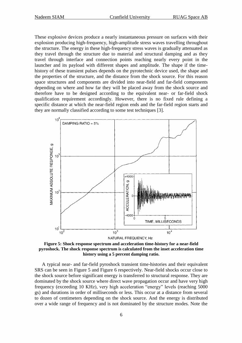
Figure 5: Shock response spectrum and acceleration time-history for a near-field

pyroshock. The shock response spectrum is calculated from the inset acceleration time

history using a 5 percent damping ratio.

A typical near- and far-field pyroshock transient time-histories and their equivalent

SRS can be seen in Figure 5 and Figure 6 respectively. Near-field shocks occur close to

the shock source before significant energy is transferred to structural response. They are

dominated by the shock source where direct wave propagation occur and have very high

frequency (exceeding 10 KHz), very high acceleration “energy” levels (reaching 5000

gs) and durations in order of milliseconds or less. This occur at a distance from several

to dozen of centimeters depending on the shock source. And the energy is distributed

over a wide range of frequency and is not dominated by the structure modes. Note the


7

nearly constant increase in the g levels throughout the frequency range as can be seen in

Figure 5. This is due to the small effect of the structural response on the original shock

pulse. Far-field shocks occur at a relatively greater distance from the shock source

where significant energy has transferred into a lower frequency structural response.

They contain lower frequencies (not exceeding 10 KHz), lower acceleration “energy”

levels of about one fifth of near-field shock (about 100 gs) and a bit longer duration

which is typically less than 20 milliseconds. Most of the energy in a far-field shock is

concentrated at one or few of the dominant structure modes [3]. A typical far-field pulse

time history and its equivalent SRS can be seen in Figure 6. As can be seen in the

figure, the transient acceleration time-history have a short period of increasing

amplitude and before it starts decaying again. This is due to the interaction of the

reflected stress wave as they return from different location in the structure. A typical

far-field SRS have an increasing acceleration levels up to the most dominant structure

mode before it starts slightly decreasing again. The point at which it reaches the peak is

called the knee frequency and is usually between 1000 and 5000 Hz as can be seen in

Figure 6 [3]. Shocks can also be classified as a mid-field shock filling the gap between

near- and far-field. They are dominated by a mixture of structural response and direct

wave propagation from the shock source and normally have similar amplitudes to far-

field shocks, similar frequencies as a near field shock and normally occurring at a

distance between dozen to several dozen of centimeters from the source depending on

the shock source.

Figure 6: A typical shock response spectrum and acceleration time-history for a far field

pyroshock. The shock response spectrum is calculated from the inset acceleration time

history using a 5 percent damping ratio. The straight lines indicate tolerance bands

(typically ±6 dB as shown) which might be applied for qualification test specification.


8

2.2 Shock Response Spectrum (SRS)

As a shock acceleration time-history is too complex, it cannot be used as a useful

shock representation tool directly. Shock Response Spectrum is found to be a more

useful tool for shock representation and comparison used by engineers. It is a calculated

function based on the transient acceleration-time history of a shock giving more

information about the maximum amplitude and the frequency content of the system

response making it easier for comparing the effect of similar shock pulses on the system

response.

Shock Response Spectrum is the most commonly used and main standard shock

environmental qualification requirements used in MIL-Standards (MIL-STD-1540C and

MIL-STD-810E) and in Space industry [4]. It contains information of the maximum

response of the structures where the component will be placed based on the transient

pulse that the structure is expected to be subjected to and independent of the structure

itself as it contains the maximum response for a wide range of natural frequencies. This

makes it an efficient qualification requirement for space structures subjected to shock

loading especially at early design stages where not enough knowledge is available for

the different spacecraft structures and their integrations. Therefore every component

depending on where it will be placed, near or far from the shock source has to be

designed to be able to survive a certain Shock Response Spectrum.

Shock Response Spectrum is a measure of the maximum response of an array of

single degree of freedom systems when their base is excited with a certain transient

pulse as can be seen in Figure 7. The base of the structure is excited with a transient

pulse, which is the acceleration time-history that needs to be studied (assuming no

mass-loading effects on the base input), as can be seen in the lower left corner in Figure

7, calculating the amplitude of the maximum acceleration response for all the

independent systems separately considering a constant damping value (normally 5%

critical damping for the array of the single degree of freedom system, Q = 10) and

plotted as a maxi-max acceleration-frequency as can be seen in Figure 7.[4]

(1)

Where:

– (2)

Figure 7: Array of single degree of freedom systems.


9

Where y is the common base input for each system, and x is the absolute response of

each system to the input. Where the dot donates velocity and the double-dot denotes

acceleration. M is the mass, K is the stiffness, C is the damping coefficient, and fn is the

natural frequency for each system.

Many transient time-histories can have the same or similar effect on the array of the

single degree of freedom system producing similar shock response spectrum for the

different excitations, therefore the original time history cannot be reproduced and have

to be stored. This is not the case with shock environmental qualification requirement

which is normally provided as a Shock Response Spectrum with certain tolerance level.

This qualification SRS is then taken to one of the shock testing facilities (like the

ringing plate) to produce a shock pulse that can match the qualification requirements

SRS within the specified tolerance level as can be seen in Figure 8. The real structure is

then subjected to this pulse and is inspected for failures and operational errors.

Figure 8: A common far-field qualification requirement SRS with its matching

reproduced SRS laboratory.

2.3 Shock Testing

Over the years, testing used to be the main qualification method for structures

subjected to shock loading used by engineers. This is due to the complex nature of

shock and stress wave propagation in structures and due to the lack of the availability of

a reliable computational shock analysis method [2]. Similar pulses to that produced by

pyrotechnic devices can be produced laboratory by sudden release of strain energies or

with metal to metal impacts [1] which can be done using many simple and complicated

test equipments. One of the most common and simple ways of reproduction of shock

pulses similar to that produced by pyro-shocks is using the ringing plate which is

explained in more details in the following section.


10

The main disadvantages of testing is that its normally done at a late stage of the

project requiring building up a mockup for the final design, testing it, then inspecting

the test object for failures, crack, or any other operational errors. This is normally done

at a late project stage making it a critical requirement as it can be expensive and time

consuming if modifications are required at this late project stage.

2.3.1 Ringing Plate

The Ringing Plate is a common and simple shock testing device that is found in

many environmental testing facilities in space industry. It is simply a table with a freely

vibrating plate on top of it as can be seen in Figure 9. The plate is placed over a thick

layer of foam to allow its free vibration. Two excitation mechanisms are attached to the

table, a pendulum mass on one side of the plate and a free falling mass through a guided

tube over the middle of the plate. The shape of the ringing plate and the mass attached

to the pendulum and the free falling mass are used to create different pulse shapes

producing different SRS depending of the required qualification requirement to be

reproduced. The pendulum mass is used to produce in-plane shock at the interface of the

test object which is placed on the other side of the ringing plate. While the free falling

guided mass is used to produce an out-of-plane shock at the test object interface (z-axis

excitation). The ringing plate is used to create similar SRS to that of the qualification

requirement. Tested structures have to survive the reproduced shock and are inspected

for failure, dislocations, and any operational errors. On the right image in Figure 9

shows the ringing plate used at RUAG Space AB in Gotheburg, Sweden which is used

for all the testing done in all of the following sections.

Figure 9: Left: Ringing plate Diagram showing the pendulum mass, the guided tube and

the plate placed over a foam layer. Right: Ringing plate used at RUAG Space AB.


11

3. SHOCK SIMULATION

There are two possible ways for shock simulation using computational methods.

Using Statistical Energy Analysis (SEA) in which the response of the system is

predicted using statistical methods depending shock source, the location where the

components will be placed and the interface points that the shock will have to travel

through based on previous studies and similar environments. This is an approximated

method which has shown reliability in some fields, especially for high frequency

contents available in shocks. The other possibility is using Finite Element Methods

(FEM) which is investigated further and in more details in this study. Finite Element

Methods discretizes big, complex models to much finer, smaller elements and solving a

set of deferential equations describing them. FEM are known for their accuracy in

simulating structures under static loading and low frequency dynamic loading, but are

known for their limited capabilities for high frequency dynamic loading. One other

possible way for shock simulation is using a combination of both the FEM with the

Statistical Energy Analysis (SEA) combining the benefits of both methods in one

method.

Finite element analysis software are known for their limited capabilities when

simulating structures under high frequency dynamic loading which is present in shocks

making them unsuitable for shock analysis [2]. This is not true as the maximum

frequency that can be simulated using FEM depends on the model accuracy, structure

complexity, material, element type and size, damping values, type of excitation and time

steps used. In addition, a good understanding of shocks and stress waves propagation in

structure is also required when simulation high frequency shocks as will be discussed

further in the following sections. MSC Nastran is the FEM solver used in this study

with MSC Patran as a pre- and post-processor whenever possible due to their

availability at RUAG Space in Gothenburg and the company requirements. In addition,

Nastran is an implicit FEM solver which is widely used in Space and Aerospace

industry making it even more suitable for this study.

3.1 Possible Simulation Methods Using FEM

Shocks are transient dynamic loads occurring for a very short period of time with

very high frequencies which can be simulated in both the time and the frequency

domain. Three types of analysis can be used in Nastran for this type of load. Frequency

Response Analysis (SOL112), Transient Response Analysis (SOL106), and SRS

Analysis using Normal Modal Analysis (SOL103) which is the recommended method in

Nastran’s users guide. Both of the Frequency Response and the SRS method can be

excited with frequency dependent loads making it possible to use the qualification

requirement SRS directly as an input to the model, where transient response analysis

can only be excited with time dependent loads. All three methods can provide output in

the frequency domain, however only Frequency response analysis can undergo all the

simulation in the frequency domain accepting frequency dependent loads and providing

frequency dependent output with full support from Patran and without any special

manual modification or addition to the bdf file. On the other hand, both of the transient

response and SRS method will require special requests and modifications to the bdf file

as they are not supported by Patran when requesting frequency dependent outputs. This


12

increases the complexity of these 2 simulation methods and requires more

understanding of shocks, shock response spectrum, as well as Nastran code for efficient

and reliable simulation predictions.

Modal super-position is used in SRS analysis using the normal modal analysis as

well as in modal frequency response and modal transient response analysis. The direct

method performs a numerical integration on the complete coupled equations of motion.

They are more accurate but required huge computational time and power compared to

modal super-position. Modal superposition is based on normal modes and mode shapes

to reduce and uncouple the equations of motion for calculating the system response. It is

much faster and more suitable for big and complex models than direct frequency or

direct transient response saving a lot of computational time and power [10]. In addition,

requesting SRS outputs using transient response analysis is only possible using modal

transient response analysis. Therefore normal modes analysis is the main and the initial

stage for all the simulation methods used in this study as will be explained in the

following sections.

3.1.1 Modal Analysis

Normal modes analysis calculates the normal modes and mode shapes for structures.

It is usually the first step for any dynamic analysis giving a basic understanding of the

dynamic behavior of the structure and its response to dynamic loading at an early stage

of the design process. In addition, normal modal analysis is the base requirement and

the first simulation step for all of the three simulation methods that can be used for

shock analysis using Nastran and are taken into consideration in this study as will be

discussed in the following sections.

Structure normal modes, also called natural frequencies or Eigen-values, are

frequencies at which the structure tends to oscillate with higher amplitudes when

excited with dynamic loading of similar frequency. If the excitation frequency reaches

one of the structure normal modes resonance will occur, if no damping is applied,

causing the structure to peak its response and will deform in a certain shape and

amplitude called mode shape or Eigenvector. Each structure mode shape is related to a

certain normal mode. Structure modes and mode shapes are functions of material

properties and structure design/shape. However, for a certain structure design/shape, if

the material properties changed the structure normal modes can change but the mode

shapes may remain unchanged for each mode. [10]

Normal modes are calculated using SOL 103 with a reduced form of the equation of

motion as can be seen in Equation 3 [10]. The number of eigenvalues and eigenvectors

is equal to the number have mass or the number of dynamic degrees-of-freedom.

– (3)

Where:

M = Mass Matrix.

K = Stiffness Matrix.

= i-th Eigen value (circular natural frequency) = .

= i-th Eigen vector (or mode shape).

Where the natural frequency in Hz is:


13

(4)

Where:

= i-th natural frequency

After calculating the normal modes and mode shapes for a linear elastic structure

under free or forced vibration, the deflected shape of the structure at any given time is a

liner combination of all of its normal modes (called modal super-position) as expressed

in Equation 5. This is one of the very useful characteristics of natural frequencies and

mode shapes for dynamic analysis which will be used in all the following simulation

methods [10].

(5)

Where:

= vector of physical displacements.

= i-th modal displacement.

All simulation methods explained in the following sections will be based on modal

super-position using Equation 5. Therefore modes have to be calculated for at least one

and half time more than the maximum simulation frequency required. Calculating

structure modes and mode shapes is the most computational time consuming step in all

the following simulation methods and therefore its recommended to request modes for

at least one and half time more than the maximum shock simulation qualification

requirement at an early stage when running the initial normal modes analysis with a

.DBALL file output request. The DBALL file will store the modes and mode shapes to

be used later in any simulations based on these results saving a lot of computational

time and power. Frequency response analysis and transient response analysis are both

based on the same method for response calculation. However on solves in the frequency

domain and the other in the time domain as will be explained in the following sections.

3.1.2 Frequency Response Analysis

Modal frequency response analysis is the simplest of all simulation methods taken

into consideration in this study. It is based on modal superposition explained earlier in

the previous section and is fully supported by patran. No manual modifications to the

bdf file produced by patran are required. In addition, the qualification requirement SRS

or the test measures SRS can be used directly as an excitation for the model.

Frequency response analysis computes structural response to steady-state oscillatory

excitation. Excitation in this analysis is explicitly defined in the frequency domain, and

all of the applied forces are known at each forcing frequency. Forces can be in the form

of applied forces and/or enforced motions (displacements, velocities, or accelerations).

The results obtained from a frequency response analysis usually include grid point

displacements, grid point accelerations, and element forces and stresses which can be

directly ploted as a function of frequency using Patran. Modal Frequency response

analysis calculates the response of the system using the reduced equation of motion in

the modal coordinates as expressed in Equation (6). [10]

(6)


14

Where:

= modal damping ratio

= modal frequency (eigenvalue)

3.1.3 Transient Response Analysis

Modal transient response analysis is based on modal superposition explained earlier

in the previous section and is also supported by patran except for Shock Response

Spectrum output requests. This makes it more complicated than modal frequency

response analysis and therefore will require some manual modifications to the bdf file

produced by patran. However when SRS output is not required, this simulation method

can be very simple when studying stress levels in a structure only. When SRS output is

required (for example when ringing plate test comparison is required), the bdf file

produced by patran will have to be modified manually adding some information about

the location where the SRS is required, output format, SRS damping for certain points,

and some modification for the file format. The output SRS produced by this method will

be in the form of a punch file which is not supported by patran and the output SRS will

have to be plotted using other software like Matlab or Excel. A sample for the bdf file

used for the simple model can be seen in Appendix A.

Transient response analysis is the most general method for computing forced

dynamic response. The purpose of a transient response analysis is to compute the

behavior of a structure subjected to time-varying excitation. The transient excitation is

explicitly defined in the time domain. All of the forces applied to the structure are

known at each instant in time. Forces can be in the form of applied forces and/or

enforced motions. The results obtained from a transient analysis are typically

displacements and accelerations of grid points, and forces and stresses in elements.

Modal transient response analysis calculates the response of the system using the

reduced equation of motion in the modal coordinates as expressed in Equation (7). [10]

(7)

Where:

= modal damping ratio

= modal frequency (eigenvalue)

3.1.4 NASTRAN’s SRS Method

This method is Nastran’s recommendation method for shock analysis and is based

on normal modals analysis using Nastran SOL103. This method is not supported by

Patran and is the most complicated simulation method requiring nearly a complete

modification to the bdf file produced by Patran using normal modes analysis SOL103.

There are three possible approximations that can be used in this method with different

levels of approximation. However all of them methods will output only the peak

response and the peak stresses of the system at the requested locations and therefore

only the peak acceleration values will be compared when simulating using this method


15

and no SRS comparison with test measurements will be possible. A sample for the bfd

file used for simulating the simple model using this method is attached to Appendix B.

This simulation method can be excited with loads in the frequency domain or more

precisely it can be excited with a SRS knowing the SRS damping value used when

calculated. This makes it the easiest method from possible excitations point of view. It

can be excited using a qualification requirements directly or test measured SRS directly

know the SRS damping value with which it was calculated.

Three possible levels of approximation can be used within this method. The

following explanation of the approximation methods are based on Nastran’s Advanced

Dynamics User Guide [ref. 11].

Using Equation (5) the actual transient response at a physical point can be expressed

by:

(8)

Where:

= displacement at time t.

= response function in direction r.

= participation factors.

= structural damping parameters.

The peak magnitudes of in Equation (8) are usually dominated by the peak

values of x(t) occurring at the natural frequencies. In spectrum analysis the peak values

of are approximated by combining functions of the peak values, , in the approximation:

(9)

ABS Method (Absolute Value option)

This method assumes the worst case scenario in which all of the modal peak values

for every point on the structure are assumed to occur at the same time and in the same

phase. Clearly in the case of a sudden impact, this is not very probable because only a

few cycles of each mode will occur. However, in the case of a long term vibration, such

as an earthquake when the peaks occur many times and the phase differences are

arbitrary, this method is acceptable [11].

A second way of viewing the problem is to assume that the modal magnitudes and

phases will combine in a probabilistic fashion. If the input loads are behaving randomly,

the probable (RMS) peak values are [11].

(10)

Where the average peak modal magnitude, is

(11)


16

SRSS Method

This approach is known as the SRSS (square root of sum-squared) method. Note

that the results in each direction are summed in vector fashion for each mode first,

followed by an SRSS calculation for all modes at each selected output quantity uk. It is

assumed that the modal responses are uncorrelated and the peak value for each mode

will occur at a different time. These results are optimistic and represent a lower bound

on the dynamic peak values. [11]

The SRSS method may underestimate the actual peaks since the result is actually a

probable peak value for the period of time used in the spectrum analysis. The method is

normally augmented with a safety factor of 1.5 to 2.0 on the critical outputs. [11]

NRL Method

As a compromise between the two methods above, the NRL (Naval Research

Laboratories) method was developed. Here, the peak response is calculated from the

following equation:

(12)

Where the j-th mode is the mode that produces the largest magnitude in the product

. The peak modal magnitudes, , are calculated with Equation (11). [11]

The rationale for the method is that the peak response will be dominated by one

mode and the SRSS average for the remaining modes could be added directly. The

results will fall somewhere between the ABS and SRSS methods [11] and therefore the

NRL method will be used in the following simulations.

3.2 Possible Excitation Methods

Different types of excitations were considered for every simulation method and

compared to ringing plate test measurements. For frequency response analysis as well as

for SRS analysis using the NRL method excitation with frequency dependent loads are

possible and therefore qualification requirement SRS as well as test measured SRS can

be used as an input loads for these two methods. The advantage of frequency dependent

loading is that the provided qualification requirement SRS can be applied directly as an

input to the model without any modifications or transformations where for time

dependent loads the qualification requirement SRS will have to be converted to a half-

sine pulse or another simple shaped pulse equivalent the qualification requirement SRS.

Transient response analysis can only be excited with time dependent loads and therefore

the test measured acceleration-time history as well as a simple half-sine pulse equivalent

to the qualification requirement SRS were taken into account as will be explained in the

following sections. All simulation methods are considered with excitation in one

direction (excitation direction) as well as in all three translation directions taking into

account the effect of wave reflections and refractions. The following excitations were

taken into account for frequency and time dependent excitation respectively.

Frequency dependent excitation (SRS input):

Used for: Frequency response analysis & NRL method


17

Qualification SRS excitation in one direction

Qualification SRS in 3 directions.

Test measured SRS in one direction.

Test measured SRS in 3 directions.

As explained earlier the original acceleration-time history of certain qualification

requirement shock response spectrum cannot be reproduced analytically, but with some

iteration a half-sine pulse or other simple pulse shapes equivalent to a certain SRS can

be produced for a certain damping value and a system with a known first mode. There

are some simple software that can reproduce a simple pulse shape that matches a certain

SRS within the required tolerance level. Therefore for a half-sine pulse equivalent to the

qualification SRS will be taken into consideration together with the test measured time

history measured at the test object interface for time dependent loads.

Time dependent excitation (Acceleration-time history input):

Used for: Transient response analysis

Qualification equivalent half sine pulse in one direction.

Qualification equivalent half sine pulse in 3 directions.

Ringing plate produced transient sine pulse in one direction

Ringing plate produced transient pulse in 3 direction.

Reflections and Refractions

Stress waves produced by shocks are reflected, refracted, and dissipated as they

travel through the structure. Stress waves reflection, refraction, and dissipation are very

complex phenomenon that cannot be easily predicted or calculated. Once a plate or a

structure is excited in one direction, stress waves will travel through the structure and

will be reflected whenever they hit another surface, screw hall or an interface in a very

complex way reaching the test object interface from all other directions as can be seen

in the ringing plate example shown in Figure 10. A triangular shaped ringing plate was

used to study the effect of reflection and refraction over the plate surface when

producing a SRS equivalent to a certain qualification requirement as can be seen in the

figure. Accelerations were measured in all 3 translation directions at the test object

interface to compare the magnitude of reflected waves compared to waves generated in

the main excitation direction. As can be seen in the figure the blue curve represents the

required reproduced SRS in the main excitation direction (y-direction) which matches

with the qualification requirement within its allowed tolerance level, where the green

and purple represents the measure SRS in the z- (out of plane) and the x-directions

respectively. As can be seen in the figure the amplitude of the reflected waves in the

other two directions are very high and are comparable to the originally reproduced SRS

in the main excitation direction and tends to get even closer at higher frequencies which

is the main concern for shocks. Therefore any excitation in only one direction

neglecting the effect of reflections and refraction will be a highly underestimation

especially for the high frequency region which is the main concern for shocks

containing the highest acceleration levels.


18

Figure 10: Test measured SRS in all translation directions (x, y, and z).

In addition, as can be seen in Figure 10, the amplitude of the reflected does not

change linearly and there is no certain pattern defining the relation between amplitude

of the reflected waves and the original reproduced pulse in the main excitation direction.

This is due to the complexity of stress wave reflection, refraction, and dissipation as

they don’t only depend on the main produced pulse. Many other different parameters

influence the amplitude of the reflected pulses like shape of the plate used, material,

and even testing conditions, test object properties and test settings and adjustments to

the ringing plate. All these parameters have a direct influence on the magnitude of the

reflected waves and therefore they cannot be calculated or predicated easily.

Qualification requirement SRS directly in 3 direction

Using the qualification requirement SRS directly as an input for the simulation with

excitation in all three translation directions required a good understanding of shock

wave propagation in the shape of the ringing plate used in the test and the test settings

and conditions for comparison with simulation prediction. This requires the amount of

reflected waves in the other two directions (other than the excitation direction) to be

known. As explained earlier the amplitude of reflected waves in other directions is very

difficult to predict due to the complexity of stress waves propagation and reflection in

the structures. This will require a good knowledge of the fraction of reflected waves

reaching the test object interface in all other direction for every plate design, produced

SRS, and test settings which will not even be an evenly distributed over the frequency

range. For this reason this excitation method is not taken any further in this simulation.

Half-sine Pulse Excitation

As explained earlier in the previous sections, the original transient acceleration-time

history for a certain qualification requirement SRS cannot be reproduced to be used as

an excitation for simulation methods accepting only time dependent loads. However for

a certain qualification requirement SRS and for a system with a known first mode a

simple excitation pulse (ex. half-sine pulse) producing similar effect on the array of the

single degree of freedom system can be produced. The peak of the pulse will depend on

the value of the peak qualification acceleration and the pulse period will depend on the

period of the system’s first mode. This simple reproduced pulse can be used as an input


19

excitation for simulation methods accepting only time dependent loads like transient

response analysis.

Using a half-sine pulse requires a structure to create the required response at the

equipment interface. This can be done by modeling a plate or a beam that can generate a

similar response at the equipment interface as can be seen in Figure 11 and Figure 12.

The plate or the beam used will have to be adjusted, modeled, meshed and added to the

equipment FEM. This adds more complexity to the structure and requires the creation of

a certain structure for every SRS qualification. In addition, the plate or the beam used to

create the response will have to be modeled and meshed with very high accuracy

increasing computational time and size. However, using the ringing plate to create a

time-history at the interface of the structure is more practical and the measured

acceleration-time history can then be stored and used for similar qualification SRS

reducing computational time and size.

Figure 11: A simple tooth shaped pulse used to excite the rectangular shaped plate shown

on the right.

Figure 12: Reproduced transient pulse.

All the excitation methods discussed are applied to simple structures and compared

to each other and to ringing plate tests proving these theories. Therefore test measured

acceleration time-history in all three translation directions (x, y, and z) and their

equivalent SRS will be used as the main excitations for the following simulation

methods.

Final chosen simulation methods with their excitation

Frequency Response Analysis Excited with a test measured SRS in 3

translation directions.

SRS Analysis using the NRL Method Excited with a test measured SRS in 3

translation directions.

Transient Response Analysis Excited with a test measured acceleration-time

history in 3 translation directions.


21

4. SIMPLE MODEL

The main idea of the simple structure is to be as simple as possible for easy and fast

manufacturing as well as for simple and fast simulation for comparison of the different

simulation methods, sanity check, calibrations, and adjustment of the different

simulation parameters and studying their effect on the simulation predictions. The

model was chosen to have a simple bracket shape as can be seen in Figure 14 and made

of a common material that in normally used in RUAG Space products. In addition, the

simple structure should have a first Eigen frequency equivalent to a common first Eigen

frequency available in RUAG products as well.

4.1 Bracket Model

The model is made of a 100*100 mm2 Aluminum plate with a thickness of 0.8 mm

which is bent from the middle by 90 degrees as can be seen in Figure 14. Four holes

were drilled in the horizontal surface of the plate for fixing it to the ringing plate.

However, holes are not equally distributed over the plate surface to match with the holes

available on the ringing plate. One other hole is drilled on the vertical plate of the

bracket with accelerometer attached to it to measure the response of the bracket at this

point as can be seen in the left circle in Figure 14.

Dimensions:

Thickness: 0.8 mm

Length: 98 mm

Width: 50 mm

Material Properties:

Material: Aerospace Aluminum 7075-T6

Density: 2810 Kg/m3

Modulus of elasticity: 71.7 GPa

Yield Strength: 503 MPa

Ultimate Strength: 572 MPa

Poisson ratio: 0.33

4.2 Ringing Plate Test

The bracket was fixed on a triangular shaped ringing plate with four screws as can

be seen in Figure 14. Four washers were added between the bracket and the ringing

plate to reduce friction and surface contact between the bracket and the ringing plate

surface as much as possible for more realistic simulation and test comparison. A 6 Kg

mass was attached to the pendulum, raised with 35°, and left for a free fall to excite the

plate in the Y-direction as can be seen in Figure 13. Three accelerometers where

attached to the ringing plate close to the model interface measuring the input

accelerations in the X, Y, and Z-directions and one accelerometer was placed on the top

of the bracket’s vertical plate measuring accelerations response of the bracket in the

excitation direction as can be seen in Figure 14.


22

Figure 13: Ringing plate with the simple structure fixed and ready for testing.

Figure 14: Simple model fixed on the ringing plate ready for testing.

Acceleration-time histories were measured using all four accelerometers attached

near to the bracket interface and the top of the bracket. Time histories measured are of

complex shapes as can be seen in Figure 15 which can only be useful as an input

excitation for transient response analysis. As explained earlier time history

measurements are not useful for comparison or studying the effect of shock and

therefore all measured time histories were converted to SRS using 5% damping

producing interface SRS and bracket top SRS as can be seen in Figure 16 and Figure 17

respectively.

Figure 15: Test acceleration-time history measured at the bracket interface in the

excitation direction (y-direction).


23

Figure 16 and Figure 17 show the equivalent SRS calculated for all four

acceleration-time histories measured near to the bracket interface and at the top of the

bracket’s vertical plate respectively. As can be seen in Figure 16, the effect of wave

reflections is relatively high compared to the main reproduced SRS in the main

excitation directions as explained earlier in the previous chapter. Interface SRS shown

in Figure 16 will be used as an input excitation for frequency response analysis and SRS

analysis using the NRL method. Where SRS calculated from time history measurements

from the top of the bracket as can be seen in Figure 17 will be used to compare

simulation predictions of the different simulation methods and studying the effect of the

different parameters on the predicted SRS.

Figure 16: Test measured SRS at the bracket interface in X, Y, and Z-Directions vs.

qualification requirement SRS with its allowed tolerance level.

Figure 17: Test measured SRS at the bracket interface vs. SRS measured at the top of the

bracket in excitation direction (Y-direction).


24

4.3 Simulation and Results Comparison

The bracket is modeled and meshed using shell elements as can be seen in Figure

18. Screw holes were connected to a point below the bracket using RBE2 elements

where constraints and loads are applied. A large concentrated mass of 107 times the

bracket mass was attached to the node, constrained in all rotational degrees of freedom,

and excited with the transient time history and SRS measurement from the ringing plate

in the x, y, and, z directions. Similarly the upper screw hole was connected using RBE2

elements to the center of the whole where a concentrated load of 3 gm which is

equivalent to the sensor mass was attached. The model was solved with modal

frequency response, modal transient response, and SRS analysis using the NRL method

with SRS requests at sensor location. The bdf files for modal transient response analysis

and SRS analysis using NRL method were modified and are attached to Appendix A

and B respectively for further details.

Figure 18: Bracket meshed and constrained.

As explained earlier in the previous chapter, normal modes analysis is the first

simulation step for any dynamic analysis. Running normal modes analysis using

Nastran SOL103, modes were requested up to 15000 Hz which is equivalent to one and

half time the maximum SRS qualification requirement frequency, the first ten modes

can be seen in Table 1. A DBALL file was requested to be used in all following

simulations that are based on normal modes analysis. In addition, structure normal

modes are very useful for SRS analysis to check the accuracy of the simulation

predictions as the structure peak responses should match with the structure normal

modes.


25

Table 1: Bracket’s first ten normal modes.

Mode

Number

Frequency

[Hz]

Mode

Number

Frequency

[Hz]

1 147 6 838

2 347 7 1050

3 624 8 1230

4 698 9 1520

5 797 10 1730

The bracket was simulated using modal transient response, modal frequency

response and SRS analysis using the NRL method. Acceleration time history predicted

using transient response analysis can be seen in Figure 19 and Figure 20 showing

simulation prediction for the input time history vs. the response at the sensor location

and the simulation prediction vs. test measurements at the sensor location respectively.

As can be seen in Figure 19 simulation prediction show good match with the test

measurements. However, as explained earlier comparing the response of the bracket

with time histories is not easy due to the complexity of the shock pulse as can be seen in

the figure. Modifying the bdf file of the modal transient response analysis as attached to

Appendix A, SRS was requested for the vertical plate sensor location using 5% SRS

critical damping which is the same damping value used in calculating the test measure

SRS. Similarly acceleration levels were requested in modal frequency response analysis

for the same point at the sensor location attached to the vertical plate and compared to

test measured SRS as can be seen in Figure 21.

Figure 19: Simulation predictions - input RED / output BLUE.


26

Figure 20: Simulation acceleration-time history predictions compared to test

measurements at the bracket’s top sensor.

As can be seen in Figure 21, modal transient response analysis shows much better

predictions compared to modal frequency response. Modal Analysis using the NRL

Method show close results to transient response when comparing stress levels as will be

discussed in the following section. However, only the maximum acceleration and stress

responses are predicted using this method and therefore no comparison over the whole

range of frequencies is possible giving an advantage to the transient response analysis.

-400

-300

-200

-100

0

100

200

300

400

0 0.01 0.02 0.03 0.04 0.05 0.06 0.07 0.08 0.09

Time (Up to 20 msec.)

Ac

ce

lera

tio

n [

g]

Test Output

Simulation Output

-400

-300

-200

-100

0

100

200

300

400

0 0.002 0.004 0.006 0.008 0.01 0.012 0.014 0.016 0.018 0.02

Time (Up to 20 msec.)

Ac

ce

lera

tio

n [

g]

Test Output

Simulation Output


27

Figure 21: Comparison between the Transient Response and the Frequency response

compared to the test results in Y-Direction.

Acceleration levels calculated using modal transient response and modal frequency

response analysis are both based on the same theory, however, one is solving in the

frequency domain and the other in the time domain as explained in the previous chapter.

Therefore simulation predicted acceleration levels using frequency response analysis

should be the same or at least very close the transient response predictions. The reason

for the under-estimated acceleration levels using frequency response analysis is due to

the critical damping value used in calculating the SRS from the test measured

acceleration-time history which influenced the input excitation directly as can be seen in

Figure 22.

Figure 22: Effect of SRS damping on calculated response spectrum.

These calculated SRS were used directly as an input for frequency response analysis

not taking into account that they are already damped with 5% and therefore resulting in

a lower system response. However using frequency response analysis consider the load

as periodic loading resulting in highly overestimated stress levels compared to stress


28

levels predicted using transient response analysis (as can be seen in Figure 23 and

Figure 24 respectively) even though the SRS excitation used is damped and of a lower

value than what’s used in transient response analysis and what the bracket is subjected

to in real life. These highly overestimated stress levels are equivalent to applying the

peak SRS acceleration as a static load to the model as can be seen in Figure 23. This can

be improved by calculating the test measured SRS using 0% critical damping to be used

in frequency response analysis. However this will increase the stress values which are

already highly over estimated using frequency response compared to transient response.

Stresses were calculated for 3 elements at the bend as it is expected to face the highest

stresses.

Figure 23: Frequency response stresses for 3 elements at the bent part on the top vs. static

load for the same elements on the bottom – both showing highly overestimated stress of

about 400 MPa.

Modal analysis using the NRL method predicts only the maximum response as can

be seen in Table 2. However, accelerations predicted using modal response solver 103

are inaccurate for all nodes close to any constraints as explained in Nastran’s Dynamic

Analysis user guide. Due to the small size of the bracket, it can be considered that the

sensor location is close to the model constraints. Therefore comparison of simulation


29

prediction using the NRL method will not be made based on acceleration levels and will

be done based on the stress levels instead.

Figure 24: Transient Response Stresses in 3 elements at the bend (Maximum about 69

MPa) – bottom image zoomed.

Table 2: Acceleration and stress levels using the NRL method.

Location Acceleration [g] Stresses [MPa]

Vertical Plate Sensor 2415 64.2

Using the test measured SRS which is calculated using a certain value of SRS

critical damping is not a problem for SRS analysis using the NRL or similar methods

explained earlier as the damping values used when calculating the input pulse can be

taken into account when modifying the bdf file as attached to appendix B.


30

Stress values predicted using transient response and the NRL method are very close

and are much smaller than those predicted from frequency response analysis as can be

seen in Figure 24 and Table 2. However, Transient response analysis have the

advantage that it can provide a full SRS output for the required frequency range which

can be very useful compared to only the maximum response which is predicted using

the NRL method. In addition to the unreliable acceleration levels predicted using the

NRL method to all elements and nodes close to any contraint as mentioned in Nastran’s

dynamic analysis user guide and as noticed in the previous example and due to the very

hard and complex modification required to the bdf file of the normal modes analysis

using SOL103 compared to the modification required for the bdf file for SRS requests

in transient response as can be seen in their bdf files attached to appendix A and B.

Transient response analysis will be chosen as the most efficient and reliable simulation

method and will be discussed into more details in the following chapter. However, as

the maximum response predicted using the NRL method for stresses and accelerations

away from any constraint appear to be correct, this method will be used to validate the

peak transient response predictions.

Before moving to the explanation of the chosen method in the next chapter, the

bracket was used to prove the theory discussed in the previous chapter. The Bracket was

excited with the qualification requirement SRS in the excitation direction only and using

the test measure SRS measurement all translation directions using the NRL method as

can be seen in Table 3 and Table 4 respectively. Three elements at the bend were used

to compare the predicted stresses using both types of excitation. As can be seen in the

following tables the predicted Von Misses stresses are underestimated with about 20%

when the bracket is excited using only one direction using the qualification requirement

SRS as an input load compared to using the test measured SRS in all three translation

directions.

The bdf of the bracket excited with the qualification requirement SRS in the

excitation direction only was modified to solve the same model using the ABS method

and the predicted stress levels for the same elements are shown in Table 5. Comparing

stresses in Table 5 with stresses in Table 3 confirms the theory explained in the previous

chapter that the ABS method assumes the worst case scenario predicting about 20%

higher stresses than the NRL method.

Table 3: Stress results using the NRL method with qualification SRS excitation in Y-

direction.

Element ID Fiber Distance [mm] Von Misses [MPa]

4362 -0.4 32.3

0.4 38.2

4409 -0.4 55.6

0.4 54.8

4459 -0.4 28.1

0.4 35.5


31

Table 4: Stress results using the NRL method with test measured SRS in X, Y, and Z-

directions.


4362 -0.4 39.5

0.4 46.0

4409 -0.4 64.2

0.4 62.8

4459 -0.4 29.2

0.4 37.1

Table 5: Stress Results using the ABS with Qualification SRS Excitation in Y-Direction.


4362 -0.4 49.9

0.4 57.1

4409 -0.4 65.6

0.4 64.1

4459 -0.4 42.4

0.4 50.3


33

5. EXPLANATION OF CHOSEN METHOD

Modal Transient Response Analysis with a complex transient acceleration-time

history excitation in three directions gives the best simulation predictions when

compared to test measurements. The complex transient pulse used as the model

excitation can be produced using the ringing plate or other shock testing devices for

every qualification requirement as a first step when the costumer environmental

qualification requirements are received. The transient pulse should be created to match

with a certain qualification requirement only in the same excitation direction. A

database with all the qualification requirement SRS and their equivalent reproduced

acceleration-time histories can be created to be easily retrieved and reused when similar

qualification SRS is required for other projects.

Figure 25: Recommended shock simulation procedure.

Acceleration-time histories can be created using the ringing plate without any

dummy or mockups. Only three accelerometers measuring accelerations in all three

translational directions will be needed where only the reproduced SRS in the excitation

direction should match with the qualification requirements with its specified tolerance

level (normally ± 6dB). When new qualification SRS is received it should be checked in

the created database for matching transient pulses, and if no good matching is found, it

should pass over to the testing facility to create a new pulse and should be added to the

database for future reference. Having a database with all the qualification requirements

and their equivalent reproduced transient pulses in the main excitation direction and

their resultant pulses in the other translation directions will save time and testing costs

to reproduce new transient pulses for new qualification requirements.

Normal modes analysis is normally the first step for any dynamic simulation done at

an early stage of the design process. At this early stage it’s recommended to request

modes up to one and half time more than the maximum qualification SRS (normally

about 15000 Hz). Running normal modes analysis for such high frequencies is the most

computational power and is the most time consuming process in the simulation,

therefore a DBALL file should be requested. The DBALL file will contain all modes

and mode shapes calculated which will be reused when running modal transient

response for shock analysis or any other simulations which is based on normal modes


34

analysis when needed, saving computational time and power required for recalculating

structure normal modes and mode shapes.

Requesting SRS output using Modal transient response analysis requires

modification to the bdf file created by patran. This modification must include a SRS

request for certain nodes, output format, and a specified SRS damping value for every

requested node. This increases the complexity of the bdf file if many nodes are required

in the analysis, and therefore it is recommended to create two separate bdf files. One

with SRS requests for certain nodes which will have to be modified manually and the

other with any other output requests other than SRS, like stresses or strains for as many

elements as required. The SRS output can be used to sanity check, adjustment, and

calibration of the simulation predictions compared to test measurements. Once the

simulation predictions are calibrated to be within the allowed tolerance level and

approved, a normal modal transient response analysis can be run with the same

parameters studying structural stresses and strains.

When comparing simulation predictions with test results the SRS damping used in

both simulation and testing should be the same (normally 5%). In addition, a critical

damping should be specified due to other surrounding effects and material properties.

The SRS damping should be only used when requesting SRS outputs solving the special

transient response analysis with the special SRS request, while the critical damping

should be used for all the dynamic simulations. Figure 26 shows the effect of different

types of damping with different values in comparison to test results.

Special consideration should be given to the model accuracy especially for

constraints and excitations, time step, type elements used, element sizes, and damping

due to their major influence on the accuracy of the simulation predictions as will be

explained in more details in the following sections.

5.1 Transient Response .bdf file & SRS Output Request

Modifications to the normal bdf file produced by PATRAN should be made for

shock analysis requesting SRS at certain nodes and SRS damping values should be

specified for every node or element specified in the file. A sample of the bdf file with

SRS requests is explained and shown below with the main parameters that need to be

added for SRS analysis, see Table 6.

Table 6: Transient response required bulk data entry for SRS analysis [11].

Bulk Data Entry Description

PARAM,RSPECTRA,0 Requests calculation of spectra.

DTI, SPSEL, 0 Header for DTI.

DTI, SPSEL, 1 Selects oscillator frequencies, oscillator damping values,

and grid points at which spectra will be computed.

FREQi Specifies oscillator damping values.

FREQi Specifies oscillator frequencies.


35

BDF File and Explanation:

sdamping = 1

method = 1

tstep = 1

spc = 2

dload = 2

displacement(plot,sort2,real)=999

velocity(plot,sort2,real)=999

acceleration(plot,sort2,real)=999

stress(plot,sort2,real,vonmises,bilin)=888

$

output(xyplot)

xgrid = yes

ygrid = yes

$

$ plot input

xtitle = time

ytitle = accel input

xyplot acce /1956253(t2)

ytitle = displ input

xyplot disp /1956253(t2)

$

$ response spectra generation

xtitle = frequency (hz)

ytitle = absolute acceleration

$

$ note: ip -- imaginary,phase -- is relative

$ note: rm -- real, magnitude -- is absolute

$

xyplot acce spectral 1 /1956253(t2rm)

xyplot acce spectral 1 /1956274(t2rm)

xypunch acce spectral 1 /1956253(t2rm)

xypunch acce spectral 1 /1956274(t2rm)

$ direct text input for this subcase

begin bulk

param post 0

param prtmaxim yes

param, prgpst, no

param, rspectra, 0

dti, spsel, 0

dti, spsel, 1, 885, 887, 1956253, 1956274

$ specify oscillator damping value (5%)

freq, 885, 0.05

$

$ specify frequencies for spectra

freq1, 887, 0, 25., 500

velocity must be requested

Requests output srs punch file for the input

node

Requests output srs punch file for the

sensor location

prints maximum output values

suppress the output singularity points

requests spectrum calculation

look at table

look at table

look at table

look at table


36

tstep 1 8129 9.77-6

$

Time function should be longer than the

solution time to avoid error!

tabdmp1 1 crit

0. .02 2000. .02 3000. .02 4000. 0.02

10000. 0.02 20000. 0.02 50000. 0.02 endt

eigrl 1 1. 15000. 0

……………..

rest of the model

……………..

modes request – should be at least one and

half time the maximum required one

5.2 Constraints and Excitations

The equipment interface points are connected with RBE’s to a point below the

instrument and a big mass with a magnitude of 106 to 10

8 of the instrument mass should

be attached to this point. The time history is then applied to this point in the x, y, and z

and should be constrained in the other rotational directions. The time step should be

9.77-6

sec to match with the time history step.

5.3 Effect of Damping

SRS damping is the constant damping value used in calculating the response of the

array of the single degree of freedom systems, as explained earlier, and should not be

confused with other viscous and structural damping. In real life testing damping is

present in the form of friction, surrounding air, dissipation and material damping. The

effect of the different damping sources in the system is hard to measure or predict and

therefore will always result in a certain error between the test measurement and the

simulation results. However, by testing and comparison a good value of damping with

the least error can be obtained. For the simple model, the effect of different types and

values of damping was compared with test measurement as can be seen in Figure 26.

The difference between simulating without SRS damping and simulating without

critical damping is big compared to test measurements as can be seen in Figure 26.

Variable critical damping with a decreasing value at high frequency show better match

with the test measurement as can be seen in Figure 26. However, adjusting the right

value of variable critical damping is hard and is highly dependent on the material,

structural dimensions and the test conditions. Constant critical damping of 2% is close

to the variable critical damping and is much easier to adjust and therefore will be used

in the following analysis.


37

Figure 26: Effect of Different Types of Damping on the Output SRS using Transient

Response Analysis (top) – variable damping value used (bottom).

The value of the critical damping is found to be the hardest part in the simulations as

it depends very much on the test conditions, temperature, surrounding area, materials

used, connection points, friction, and heat dissipations making it very difficult to

predict. But based on experience it was found that a value of 2% give a reasonable

results. However, dealing with thin material the damping value should be decreased at

higher frequencies. Damping can also be known by some dynamic tests measuring the

behavior of the material at different frequencies, but this will be complicated due to the

variety of materials that can be used and their dimensions.

In the bracket model the simulation results were found to match more with the test

results using variable damping with about 2% critical damping up to 2000Hz and as low

Effect of Different Types of Damping on the Output SRS Using Trensient Response

Analysis

10.0

100.0

1000.0

10000.0

10 100 1000 10000

Frequency [Hz]

Ac

ce

lera

tio

n [

g]

No SRS Damping Test Output No CRIT Damping SRS Damp + 0.1 CRIT Damp Variable CRIT Damping

Critical Damping Value

0

0.2

0.4

0.6

0.8

1

1.2

1.4

1.6

1.8

2

100 1000 10000 100000

Frequency [Hz]

Da

mp

ing

[%

]


38

as 0.05% above 2000Hz. But when simulating the KU-Band Converter (the real life

model) it was found that the same values of variable critical damping give very high

values at the less damped frequency regions. This can be due to the difference of the

material thickness and the fact that the simple model was made of a 0.8 mm thick

aluminum sheet and the real life model is made of stronger and better grade aluminum.

Making it easily affected with the very low damping values.

Instrument calibrations can be done to determine the level of critical damping that

can be used in the simulation for a certain instrument. Once the calibration is done using

the SRS requests in the Transient response analysis, a normal Transient response can be

done. If no calibration was done for a certain instrument to determine the critical

damping that can be used, a variable critical damping with a very low damping values at

higher frequencies can be applied for objects with low Eigen frequencies while a

constant damping value can be applied for object with high Eigen frequencies.

5.4 Element Type and Size

The maximum frequency that can be simulated with FEM is dependent on the

element size and the maximum distance between nodes in order to fully sample/capture

the travelling wave in the structure. The waves will travel through the structure as

longitudinal tensile and compression stress waves, shear waves, and flexural waves. The

maximum allowable element size can be calculated with simple calculations based on

the shock wave velocity in the material, the maximum frequency required and the

sampling rate. The sampling rate must be at least 5 times per cycle to be able to fully

reproduce the pulse shape. The maximum distance between nodes should be calculated

for all types of waves travelling through the structure and the minimum distance should

be used.

For example for longitudinal waves, the wave length of the maximum frequency

required can be given by the following equation:

λ = V/ƒ (13)

Where V is the speed of shock wave propagation in a specified material and can be

expressed as:

V = (E/ρ)0.5

(14)

Where E is the material’s Young Modulus and ρ its density.

Therefore the minimum wave length will be

λ < (E/ρ)0.5

/ƒ (15)

For 5 sampling points within every wave length

Therefore, dmax = (E/ρ)0.5

/4ƒ (16)

Similarly for shear and flexure waves the wave length will be for shear waves:

λ < (G/ρ)0.5

/ƒ (17)

Where G is the shear modulus of elasticity.


39

For flexure waves:

λ = (2π/ƒ)1/2

(D/µ)1/4

= (2π/ƒ)1/2

(Et2/12 ρ)

1/4 (18)

Where D is the bending stiffness, and µ is the mass per unit surface area.

Only flexural waves are dispersive, i.e. flexural wave celerity expression depends

directly from the frequency.

For example using the above equations if the maximum frequency required in the

simulation is 10 000 Hz, the maximum distance between nodes for aluminum is 127.3

mm and for steel is 126.6 mm. These element sizes are relatively big compared to the

element sizes currently used at RAUG and therefore this shouldn’t cause any problems

for the current models, but it will have to be considered when simulating large

structures like big reflector antennas built by RUAG. To prove this theory the bracket

was simulated with different element sizes and compared as can be seen in Figure 28.

As can be seen in the plot, the very fine mesh is overlapping with the small mesh and

the difference between the small mesh and the big mesh can be negligible. However,

simulating the bracket with 3D elements gives much better results over the fine shell

elements mesh as can be seen in Figure 29.

Figure 27: Bracket meshed with different element sizes.


40

Figure 28: Effect on element size on the simulation results for the Bracket.

Combining the effect of element type, size, and the effect of damping the simulation

results can be highly improved as can be seen in Figure 30. The plot shows the test

measurement compared with simulation results with a ± 2 dB tolerance on the test

results for comparison. The bracket is simulated with 3D elements (tet10) and 2%

critical damping.

Figure 29: 3D elements (tet10) vs. shell elements.

10

100

1000

10000

10 100 1000 10000

Frequency [Hz]

Ac

ce

lera

tio

n [

g]

Test OutputBIG MeshSmall MeshVery Fine Mesh

Effect of Different Types of Damping on the Output SRS Using Trensient Response

Analysis

10.0

100.0

1000.0

10000.0

10 100 1000 10000

Frequency [Hz]

Accele

rati

on

[g

]

Test OutputShell Elements3D Elements


41

The model is recommended to be meshed entirely using 3D elements (for example

TET10 or TET 16 or higher) for better simulation predictions as close to reality as

possible and to avoid the inaccurate peaks with 2D elements noticed earlier when

simulating the simple model. The maximum distance between nodes should be

calculated as explained in the previous section and its value will determine the

maximum frequency that can be simulated accurately.

Figure 30: Simulation results compared to test results after adjusting the element type,

size, and damping.

10

100

1000

10000

10 100 1000 10000

Frequency [Hz]

Ac

ce

lera

tio

n [

g]

Test ResultsSimulation Results± 2 dB


43

6. REAL LIFE MODEL

Converters are one of the main products produced by RAUG Space AB in

Gothenburg, Sweden. The KU-band down-converter is a very complex and very

compact structure with PCBs and a sensitive crystal which makes it an interesting

structure to study the effect of shocks on and to compare with FEM predictions. In

addition, the PCB used in the converter with its sensitive crystal is very critical to

shocks and are of a main concern to RUAG Space.

6.1 KU-Band Converter Model

The converter’s CAD model can be seen in Figure 31 with the PCB inside showing

the sensitive crystal location. For testing a mock up was built for the converter and the

sensitive crystal was replaced with an accelerometer measuring accelerations which the

crystal will be subjected to. The rest of the PCB components were replaced with nuts of

different sizes and weights equivalent to each component and the PCB was tested using

a shaker to check the mockup PCB Eigen-frequencies compared to the original PCB

Eigen-frequency which was also tested using laser sensors as can be seen in Figure 32.

Figure 31: Converter CAD model showing sensitive crystal and measurement location.

Figure 32: Shaker test setup for the original PCB modes search on the left – the modified

mockup PCB on the right with the crystal replaced with an accelerometer.


44

6.2 Ringing Plate Test

The Converter was tested to a near field shock as can be seen in Figure 34. The

mock up was attached to the ringing plate with the test setup as can be seen in Figure

33. The plate was excited using both the mass pendulum and the free falling mass

producing in-plane pulses and out-of-plane pulses respectively testing the converter in

the Y, X, and Z-directions respectively as can be seen in Figure 33. The mockup was

fixed directly to the ringing plate without any washers underneath according to the

qualification approved testing procedures. This increases friction and surface-to-surface

contact between the plate surface and the converted which cannot be modeled easily

using FEM and is expected to cause some error when comparing test measurements

with simulation predictions. Three accelerometers were attached to the ringing plate

very close to the converter interface measuring input acceleration that the converter will

be subjected to in the y, x, and z-directions which will be used as input excitation for the

following simulation. In addition accelerations were measured with the accelerometer

placed in the crystal location measuring acceleration in y-direction only in all three

tests.

Figure 33: Shock test set-up in Y, X, and Z-directions respectively.

Figure 34: Converter’s near field qualification requirement with the matching reproduced

SRS using the ringing plate.

100 1000 1,016e+004

[Hz]

10

100

1000

1e+004

[g]

Chan.no: 2

Chan.type: M

Unit: g

-- Pulses on act. level --

done: 0

-- Pulses total --

done: 5

Date: 18.04.08

Time: 08:01:22

Y-axis (SRS: d=5,00%)Transient Capture

C:\VcpNT\Daten\PT-qual\Mjuk kristallmontering\Shock Y-_002.rtc

Mjuk kristallmontering

RTVs

Shock Y-


45

6.3 Simulation and Results Comparison

The converter’s FEM model was meshed entirely using 3D elements with a skin of

shell elements except for the PCB which was meshed using shell elements only as can

be seen in Figure 35. The PCB mesh was approximated and the overall mass of the PCB

and its components was distributed over the PCB mesh. While the stiffness of the

different PCB components was approximated with one global stiffness value over the

whole PCB. This is a rough approximation which is validated normal modes analysis

and vibration tests for both the original PCB and the mockup PCB with the senor placed

in the crystal location. As can be seen in Table 7 the first mode calculated for the

approximated PCB falls somewhere between the original PCB’ and the mock up PCB’s

first modes. This PCB modeling approximation was accepted. However, it’s expected to

cause some error when comparing simulation predictions with test measured

accelerations.

Table 7: PCB first mode compared to test measured mode using laser measurement and

accelerometer placed in the crystal location.

Mode Number

Test First

Mode (Laser

Sensors)

Test First Mode

(Accelerometer) Simulation

First Mode

1 1400 1290 1321

Figure 35: KU-Band Converter Finite Element Model.

The converter interface was connected with RBE2 elements to a point below the

model to which a large mass of 107 time the converter mass was attached and was

constrained in all rotational degrees of freedom and excited with the test measured

acceleration-time history in the x, y, and z directions. Normal modes analysis was

solved using Nastran SOL103 as a simulation first step as recommended in the previous

section with a DBALL file request. Modes were requested up to 15000 Hz to be used

when running modal transient response and to validate the predicted and test measured

peak response of the converted. Normal modes analysis was done for the PCB

separately to as the accelerometer will be attached to it and due to its major influence in

the predicted response. Table 8 and Table 9 show the first 15 and 10 modes for the

converter and the PCB respectively with the first 3 PCB mode shapes as can be seen in

Figure 36.


46

Table 8: Converter’s first fifteen normal modes.

Mode

Number

Eigen

Frequency

Mode

Number

Eigen

Frequency

Mode

Number

Eigen

Frequency

1 497 6 1370 11 1860

2 600 7 1500 12 1950

3 962 8 1600 13 2010

4 1310 9 1610 14 2090

5 1360 10 1630 15 2210

Table 9: PCB’s first ten modes.

Mode

Number Frequency

Mode

Number Frequency

Mode

Number Frequency

1 1321 4 2729 8 5001

2 2008 5 3338 9 5340

3 2493 6 4221 10 5557

4 2729 7 4371

Figure 36: First three PCB mode shapes.

Figure 37, Figure 38, and Figure 39 show the simulation predicted SRS compared to

the test measurements at the crystal location for y, x, and z excitation respectively. Test

measurements and simulation predictions are taken in the y-direction from the crystal

location on the PCB for all y, x, and z-direction excitations. A ±3 and ±6 dB tolerance is

added to the test measurement for easier comparison with the simulation predications

error level.

As can be seen in Figure 37 simulation predictions matches very well with test

measures SRS and mostly within ±3dB tolerance level. Only exceed 6dB for a very

small frequency range between 4 and 5 KHz. This error in simulation prediction can be

due to the approximation in the PCB modeling in which a the global mass of the PCB

with its components was distributed over the whole PCB, in addition to the global

stiffness which was added to the PCB as an approximation for the stiffness of its

components. In addition, the PCB was meshed using 2D shell elements which are not

accurate so accurate when simulating shock as explained in the previous chapter. As can

be seen in Figure 37, all peaks in the error region exceeding +6dB matches with the

PCB 5th

, 6th

, and 7th

modes as shown in Table 9. This confirms that the PCB modeling

approximation is the most likely reason for this error. Therefore simulation predictions

is expected to improve significantly with better and more accurate modeling for the

PCB and its components and by using 3D elements instead of the currently used 2D

elements.


47

Figure 37: Test results vs. simulation predictions in the Y-direction.

Other sources of error can be due to friction and surface-to-surface contact between

the converter and the ringing plate during the test which was not taken into account in

the converter simulation for simplicity reasons. However, this can be improved by

retesting the converter model with washers placed at the converter interface between the

converter and the ringing plate decreasing surface contact and friction and producing

more realistic simulation and testing comparison. Although these are simple

modification that can improve the simulation predictions significantly, they were not

applied due to the limited ringing plate test availability and time limits.

Yet with all these possible error sources, the in-plane simulation prediction shows

very good predictions compared to the test measurements which is mostly below ± 3dB

for the X-direction (Figure 38) and exceeding +6dB for a very small frequency range

for the Y-direction (Figure 37).

Out-of-plane excitation (z-direction) as can be seen in Figure 39 show more error

than in plane excitations shown in Figure 37 and Figure 38. Z-direction simulation was

done at a very late stage of this study and therefore there was not enough time for

further modifications to try to improve or decrease this high error levels. However, for

out of plane excitation, and similarly to previous in-plane excitations, acceleration

measurements were taken from the PCB at the crystal location measuring acceleration

in the y-direction which is placed at a certain distance above the ringing plate. Therefore

error in this case is highly possible to be due to the cross-axis simulation for which the

excitation is z-direction and the measurements are in the y-direction at the crystal

location on the PCB. For this time of simulation rotational degrees of freedom will play

a major role in the accuracy of the simulation predictions and results can be improved

by trying to take into account flexure waves in the ringing plate through measuring the

rotational acceleration at the converter interface especially around x, and y, axis and

applying it as an extra excitation to the model in addition to the currently used

Converter's SRS Measurements vs. Simulation at the Crystal Location

10

100

1000

10000

100000

100 1000 10000Frequency [Hz]

Ac

ce

lera

tio

n [

g]

Test ResultsSimulation Results - 2% Critical DampingSRS Response Using NRL Method±6 dB±3 dB


48

transitional direction excitations. This is in addition to using shell elements for the PCB

modeling.

Figure 38: Test results vs. simulation predictions in the X-direction.

Figure 39: Test results vs. simulation predictions in the Z-direction.

Summary of Possible Error Sources and Possible Simulation Improvements:

- Inaccurate PCB material properties.

- PCB components not modeled.

- PCB using 2D elements.

- Surface contact and friction between the converter and the ringing plate.

10

100

1000

10000

100000

100 1000 10000

Frequency [Hz]

Ac

ce

lera

tio

n [

g]

Simulation ResultsTest Measurments±6db±3dB

10

100

1000

10000

100000

100 1000 10000

Frequency [Hz]

Ac

ce

lera

tio

n [

g]

Simulation ResultsTest Measurments±6 dB±3 dB


49

7. FURTHER WORK

- Generation of transient acceleration-time history pulses using the ringing for the

different qualification requirement SRS creating a database for easy and fast access

providing transient excitation pulses for every qualification requirement SRS which can

be used as an input for the simulation model.

- Studying the maximum distance between test object interface points or test object

maximum size from which different input excitations will have to be taken into account.

- Development of a more reliable and efficient PCB modeling technique taking into

account the stiffness of the different PCB components and their masses.

- Studying the damage potential for structures subjects to shocks which normally face

high stress levels exceeding the maximum allowable yield and ultimate limits. However

these stresses occur for a very short period time which is usually fast enough and may

only cause very small deformation in metallic materials that can be neglected causing

no serious damage or failure to structures. This can be based on the energy contents of

the shock or can be studied using the structure velocity response as velocity is the

parameter of greatest interest from the viewpoint of damage potential. This is because

the maximum stresses in a structure subjected to a dynamic load typically are due to the

responses of the normal modes of the structure, that is, the responses at natural

frequencies. At any given natural frequency, stress is proportional to the modal

(relative) response velocity [2].

- More detailed in-depth study of the damping effect and critical damping values that

can be used when simulating different structures with different materials, different

shapes and dimensions.


51

8. CONCLUSION

Dynamic loads are the main concern for space structures with their variety and

extreme loading conditions. Dynamic loading vary from periodic loading to

acoustic/random vibration and shocks. Shock in space structures are produced by

pyrotechnic devices placed in the launchers initiating the stage separations, in

addition, other less intense shock sources can be the deployment mechanisms for

solar cells, antennas, and other satellite components. These high intensity shocks are

of a main concern for sensitive space structures, like PCBs, crystals, and fragile

optical components and therefore are of a main concern for satellite components

suppliers like RUAG Space.

Space structures qualification requirements are normally provided as a Shock

Response Spectrum (SRS) with certain tolerance level. Structures have to be tested

using the ringing plate or any similar shock testing device producing a transient

shock pulse matching with the qualification requirement SRS within its tolerance

level and the structure should be inspected for any deformation, failure, or any

operational error. Shock testing is normally done at a late project stage making it a

critical project requirement causing delays and increasing project costs if

modifications are required at this late stage. Testing used to be the main method for

studying the effect of shocks on structures and components due to the lack of an

efficient computational shock simulation method. However, with the increasing

shock intensity in launchers due to the decreased amount of damping materials, and

the increasing customer qualification requirements, the possibility of simulating

shocks using Finite Element Models (FEM) has been studied. Different simulation

methods have been investigated, applied to a simple structure as well as a more

complex electronic equipment and compared with ringing plate test measurements.

All possible simulation methods that can be used for shock simulation available

in Nastran were taken into consideration. Comparing modal frequency response,

modal transient response, and Shock analysis using the NRL method which is

Nastran’s recommended shock simulation method with test measured SRS, modal

transient response analysis with test measured acceleration-time history excitation in

all three translational directions or more would be the best shock simulation method.

This requires the qualification requirement SRS to be converted to an equivalent

acceleration-time history using the ringing plate or any similar shock testing device

measuring the equivalent time history in the main excitation directions as well as the

reflected pulses in as many directions as possible to be used as the simulation input

excitation. Due to the high frequency contents available in shock, the accuracy of

shock simulation predictions is highly dependent on the model accuracy, type of

excitations and constraints as well as to the element type, size and the damping

values which are a major factor limiting the maximum frequency that can be

simulated using FEM. Taking into account these main considerations and with

accurate and detailed modeling, shock simulation for the simple bracket as well as

for the more complex converter model show good SRS predictions compared to test

measured SRS. Therefore shock simulation using FEM is possible.


52

9. REFERENCES

1. P. L. Walter. Pyroshock Explained, PCB Piezotronics, Dephue, New York.

2. Harris C.M. and Piersol, A. G. (eds.) (2002), Harris' Shock and Vibration

Handbook, 5th Edition, McGraw-Hill. Chapter 23.

3. Harris C.M. and Piersol, A. G. (eds.) (2002), Harris' Shock and Vibration

Handbook, 5th Edition, McGraw-Hill. Chapter 26, Part 2, P. 26-22.

4. Tom Irvine. (2009), An Introduction to the Shock Response Spectrum, Revision Q.

5. THOMSON, W. (1993), Theory of vibration with applications (4th revised and

enlarged edition).

6. De Benedetti, M., Garofalo, G., Zumpano, M. and Barboni, R. (2007), "On the

damping effect due to bolted junctions in space structures subjected to pyro-shock",

Acta Astronautica, vol. 60, no. 12, pp. 947-956.

7. * RUAG Space – Vibration test of shock isolated oscillator board (D-G-NOT - D-

G-NOT-01198-SE - 1 - 1)

8. * RUAG Space – Shock test of shock isolated oscillator (D-G-NOT - D-G-NOT-

01219-SE - 1 - 1)

9. * RUAG Space – Antenna report

10. MSC NASTRAN Basic Dynamics User Guide, 2005

11. MSC NASTRAN Advanced Dynamics User Guide, 2005

12. MSC NASTRAN Quick Reference Guide, 2005

* Confidential documents from RUAG Space AB with restricted access. For more

information contact RUAG Space AB, Göteborg, Sweden.


53

10. BIBLIOGRAPHY

1. Caesar, B. and Vogel, F. (1996), "Structural verification of the CLUSTER four

satellite stack", European Space Agency, (Special Publication) ESA SP, , no. 386

PART 3, pp. 1209-1215.

2. Pyroshock Testing Criteria (May 18, 1999) NASA Technial Standrad, NASA-STD-

7003, Space Administration.

3. Grzeskowiak, H. and Valente, M. (2003), "Fem model (implicit modal

superposition) of an electronic equipment submitted to pyro shocks", pp. 428.

4. Kim, H. -., Woo, S. -., Kim, Y. K. and Moon, S. -. (2003), "Development of shock

testing m/c to simulate pyro-technic device explosion of space vehicle", pp. 202.

5. Shi, Q., Ando, S., Seko, H., Nagahama, K. and Saegusa, H. (2004), "The

summarization of pyro-shock testing data and SRS level prediction methodology",

pp. 549.

6. Somanath, S., Krishnan Kutty, V. K. and Francis, E. J. (2001), "Dynamics

simulation of pyro actuated 'Ball Lock' separation system for micro-satellites to

evaluate release shock", pp. 199.

7. Sutra, M., Mesnier, D., Berlioz, A. and Combes, B. (2005), "Development of a

simulation process of the behaviour of space equipment subjected to pyrotechnic

shocks, based on characterization and environmental tests", pp. 243.


A

11. APPENDIX

11.1 Appendix A – Simple Model Transient Response bdf File

$ NASTRAN input file created by the Patran 2007 r2 input file translator

$ on March 22, 2010 at 14:38:21.

$ Direct Text Input for Nastran System Cell Section

$ Direct Text Input for File Management Section

$ Linear Transient Response Analysis, Modal Formulation, Database

SOL 112

$ Direct Text Input for Executive Control

CEND

TITLE = MSC.Nastran job created on 16-Mar-10 at 11:20:28

ECHO = NONE

RESVEC = NO

SET 999 = 1 3

SET 888 = 4459 4409 4362

LOADSET = 1

$ Direct Text Input for Global Case Control Data

SDAMPING = 1

SUBCASE 1

TITLE=This is a default subcase.

METHOD = 1

TSTEP = 1

SPC = 2

DLOAD = 2

DISPLACEMENT(PLOT,SORT2,REAL)=999

VELOCITY(PLOT,SORT2,REAL)=999

ACCELERATION(PLOT,SORT2,REAL)=999

STRESS(PLOT,SORT2,REAL,VONMISES,BILIN)=888

$

OUTPUT(XYPLOT)

XGRID = YES

YGRID = YES

$

$ PLOT INPUT

XTITLE = TIME

YTITLE = ACCEL INPUT

XYPLOT ACCE /1(T2)

YTITLE = DISPL INPUT

XYPLOT DISP /1(T2)

$

$ RESPONSE SPECTRA GENERATION

XTITLE = FREQUENCY (HZ)

YTITLE = ABSOLUTE ACCELERATION

$

$ NOTE: IP -- IMAGINARY,PHASE -- IS RELATIVE

$ NOTE: RM -- REAL, MAGNITUDE -- IS ABSOLUTE


B

$

XYPLOT ACCE SPECTRAL 1 /1(T2RM)


XYPUNCH ACCE SPECTRAL 1 /1(T2RM)


$ Direct Text Input for this Subcase

BEGIN BULK

PARAM POST 0

PARAM PRTMAXIM YES

PARAM, RSPECTRA, 0

DTI, SPSEL, 0

DTI, SPSEL, 1, 885, 887, 1, 3, 4459, 4409, +DTI1

+DTI1, 4362

$ SPECIFY OSCILLATOR DAMPING VALUE (5%)

FREQ, 885, 0.05

$

$ SPECIFY FREQUENCIES FOR SPECTRA

FREQ1, 887, 0, 25., 500

TSTEP 1 8192 9.77-6

TABDMP1 1 CRIT

0. .02 50000. .02 ENDT

EIGRL 1 1. 30000. 0

$ Direct Text Input for Bulk Data

$ Elements and Element Properties for region : CM_UP

CONM2 9558 1 .0033

$ Elements and Element Properties for region : CM_Down

CONM2 9559 3 2.16+6

-------------REST OF THE MODEL-------------

$ Loads for Load Case : Trensient

SPCADD 2 1 3 4 5

TLOAD1 6 7 ACCE 1

LSEQ 1 7 8

SPCD 8 3 1 9.81

TLOAD1 9 10 ACCE 2

LSEQ 1 10 11

SPCD 11 3 2 9.81

TLOAD1 12 13 ACCE 3

LSEQ 1 13 14

SPCD 14 3 3 9.81

DLOAD 2 1. 1. 6 1. 9 1. 12

$ Displacement Constraints of Load Set : Fixed_Rot

SPC1 1 456 3

$ Displacement Constraints of Load Set : ACC_Pulse_X

SPC1 3 1 3

$ Displacement Constraints of Load Set : ACC_Pulse_Z

SPC1 4 3 3

$ Displacement Constraints of Load Set : ACC_Pulse_Y

SPC1 5 2 3


C

$ Referenced Dynamic Load Tables

$ Dynamic Load Table : TH_X

TABLED1 1

* -.00799902 -5.626 0. -5.626

* 9.77-6 -5.79563 1.95-5 -6.36106

2.93-5 -6.120753.91-5 -6.149024.88-5 -7.039575.86-5 -5.32915

6.84-5 -6.290387.81-5 -5.216078.79-5 -6.332799.77-5 -6.00767

* 1.07422-4 -5.00403 1.17187-4 -6.34692

* 1.26953-4 -4.91922 1.36719-4 -6.58723

* 1.46484-4 -5.59773 1.5625-4 -5.11712

-------------REST OF THE TABLES-------------


D

11.2 Appendix B – Simple Model NRL Method bdf File


$ on March 24, 2010 at 09:20:37.



$ Normal Modes Analysis, Database

SOL 103


CEND

TITLE = MSC.Nastran job created on 16-Mar-10 at 11:20:28

ECHO = NONE

$LOADSET = 1

SET 999 = 1 3

SET 888 = 4459 4409 4362


$SUBCASE 1

$ TITLE=This is a default subcase.

METHOD = 1

SPC = 1

DLOAD = 2

SDAMP = 2

VECTOR = 999

ACCELERATION = 999

STRESS = 888


BEGIN BULK

PARAM,AUTOSPC,YES

PARAM,SCRSPEC,0

PARAM,OPTION,NRL

$PARAM,CLOSE,1.

PARAM POST 0

PARAM PRTMAXIM YES

SUPORT, 3, 123

TABDMP1 2 CRIT

0. .05 30000. .05 ENDT

EIGRL 1 0.1 30000. 0

$ Direct Text Input for Bulk Data

$ Elements and Element Properties for region : CM_UP

CONM2 9558 1 .0033

$ Elements and Element Properties for region : CM_Down

CONM2 9559 3 2.16+6

-------------REST OF THE MODEL-------------

$ Loads for Load Case : Modal

SPC1 1 456 3

DLOAD, 2, 1., 9.81, 1, 9.81, 2, 9.81, 3

$


E

$DTI, SPECSEL, 0

DTI, SPECSEL, 1, , A, 11, 0.05

DTI, SPECSEL, 2, , A, 12, 0.05

DTI, SPECSEL, 3, , A, 13, 0.05

$



$ Dynamic Load Table : SRS_In_X

TABLED1 11

1.0 0.0 50. 11.2424 52.9732 11.3611 56.1231 11.6572

59.4604 12.018 62.9961 12.2597 66.742 12.4479 70.7107 12.6085

-------------REST OF THE TABLE-------------

$ Dynamic Load Table : SRS_In_Y

TABLED1 12

1.0 0.0 50. 34.8181 52.9732 37.2534 56.1231 40.6188

59.4604 43.4312 62.9961 46.6139 66.742 50.1576 70.7107 54.156

-------------REST OF THE TABLE-------------

$ Dynamic Load Table : SRS_In_Z

TABLED1 13

1.0 0.0 50. 22.2932 52.9732 25.9294 56.1231 30.467

59.4604 35.1563 62.9961 39.7744 66.742 45.2835 70.7107 50.3555

-------------REST OF THE TABLE-------------

$ Referenced Coordinate Frames

ENDDATA


F

11.3 Appendix C – Converter Transient Response bdf File


$ on May 26, 2010 at 16:02:57.



$ Linear Transient Response Analysis, Modal Formulation, Database

SOL 112


CEND

TITLE = JOB CREATED BY MSC_RANDOM

ECHO = NONE

MPC = 26286678

SET 999 = 1956253 1956274

$SET 888 = 2481526 375389 375464

LOADSET = 1


SDAMPING = 1

SUBCASE 1

TITLE=This is a default subcase.

METHOD = 1

TSTEP = 1

SPC = 2

DLOAD = 2

DISPLACEMENT(PLOT,SORT2,REAL)=999

VELOCITY(PLOT,SORT2,REAL)=999

ACCELERATION(PLOT,SORT2,REAL)=999

$ STRESS(PLOT,SORT2,REAL,VONMISES,BILIN)=888

$

OUTPUT(XYPLOT)

XGRID = YES

YGRID = YES

$

$ PLOT INPUT

XTITLE = TIME

YTITLE = ACCEL INPUT

XYPLOT ACCE /1956253(T2)

YTITLE = DISPL INPUT

XYPLOT DISP /1956253(T2)

$

$ RESPONSE SPECTRA GENERATION

XTITLE = FREQUENCY (HZ)

YTITLE = ABSOLUTE ACCELERATION

$

$ NOTE: IP -- IMAGINARY,PHASE -- IS RELATIVE

$ NOTE: RM -- REAL, MAGNITUDE -- IS ABSOLUTE

$


G






BEGIN BULK

PARAM POST 0

PARAM PRTMAXIM YES

PARAM, PRGPST, NO

PARAM, RSPECTRA, 0

DTI, SPSEL, 0

DTI, SPSEL, 1, 885, 887, 1956253, 1956274

$ SPECIFY OSCILLATOR DAMPING VALUE (5%)

FREQ, 885, 0.05

$

$ SPECIFY FREQUENCIES FOR SPECTRA

FREQ1, 887, 0, 25., 500

TSTEP 1 8129 9.77-6

TABDMP1 1 CRIT

0. .02 2000. .02 3000. .02 4000. 0.02

10000. 0.02 20000. 0.02 50000. 0.02 ENDT

EIGRL 1 1. 15000. 0

-------------REST OF THE MODEL-------------

$ Loads for Load Case : Trensient_Response

SPCADD 2 1 3 4 5

TLOAD1 6 7 ACCE 1

LSEQ 1 7 8

SPCD 8 1956253 1 -9.81

TLOAD1 9 10 ACCE 2

LSEQ 1 10 11

SPCD 11 1956253 2 9.81

TLOAD1 12 13 ACCE 3

LSEQ 1 13 14

SPCD 14 1956253 3 9.81

DLOAD 2 1. 1. 6 1. 9 1. 12


SPC1 1 456 1956253

$ Displacement Constraints of Load Set : Acc_X

SPC1 3 1 1956253

$ Displacement Constraints of Load Set : Acc_Y

SPC1 4 2 1956253

$ Displacement Constraints of Load Set : Acc_Z

SPC1 5 3 1956253


$ Dynamic Load Table : TH_X

TABLED1 1

* -.00799902 -2.96485 0. -2.96485

* 9.77-6 -3.40408 1.95-5 -3.15701


H

2.93-5 -3.157013.91-5 -3.088384.88-5 -3.733515.86-5 -3.43154

6.84-5 -4.1453 7.81-5 -2.9923 8.79-5 -3.911959.77-5 -3.84332

* 1.07422-4 -3.36291 1.17187-4 -3.80214

* 1.26953-4 -3.15701 1.36719-4 -4.40609

* 1.46484-4 -3.66488 1.5625-4 -4.13157

* 1.66016-4 -3.95313 1.75781-4 -3.55507

* 1.85547-4 -3.74724 1.95313-4 -3.51389

* 2.05078-4 -3.37663 2.14844-4 -2.89622

* 2.24609-4 -2.84131 2.34375-4 -3.17074

* 2.44141-4 -2.58052 2.53906-4 -3.22564

* 2.63672-4 -2.69033 2.73438-4 -3.08838

* 2.83203-4 -3.32173 2.92969-4 -4.21393

* 3.02734-4 -3.23937 3.125-4 -3.37663

* 3.22266-4 -3.00603 3.32031-4 -3.12956

* 3.41797-4 -3.54135 3.51563-4 -3.39036

* 3.61328-4 -4.5159 3.71094-4 -3.58252

* 3.80859-4 -3.06093 3.90625-4 -3.22564

* 4.00391-4 -3.52762 4.10156-4 -3.18447

-------------REST OF TABLES-------------

2010:078 master's thesis development of an efficient ...1023156/fulltext01.pdf · 2010:078...

Documents