introduction€¦ · · 2012-01-03into fuzzy logic. an introduction to fuzzy control appears in...
TRANSCRIPT

1
INTRODUCTION
MOJamshidiUniversity of New Mexico
One of the more popular new technologies is “intelligent control,” which is defined as acombination of control theory, operations research, and artificial intelligence (AI). Amongmany possible new technologies based on AI, fuzzy logic is now perhaps the mostpopular area, judging by the bfllions of dollars worth of sales and close to 2000 patentsi.wued in Japan alone since the announcement of the frost fuzzy chips in 1987. Thanks totremendous technological and commercial advances in fuzzy logic in Japan and othernations, today fuzzy logic is enjoying an unprecedented popularity in the technologicaland engineering fields including manufacturing. Fuzzy logic technology is now beingused in numerous consumer and electronic products and systems, even in the stik marketand medical diagnostics. The most important issue facing many industrialized nations inthe next several decades will be global competition to an extent that has never before beenposed. The arms race is diminishing and the economic race. is in full swing. Fuzzy logicis but one such front for global technological, economical, and manufacturingcompetitions. An equally or perhaps much more important aspect of this new surge ofinterest in fuzzy logic is the educational aspect of fuzzy logic and fuzzy logicapplications, including control systems. The purpose of this book is to describe oneexperience in the education of engineering students at the University of New Mexicow) over a span of two years. The book will first provide some basic concepts offuzzy set theory (Chapter 2), fuzzy logic (Chapter 3), fuzzy control (Chapters 3 and 4),and fuzzy logic software and hardware (Chapter 6). Then a number of actual software and
1

2 Chap.1 Introduction
hardware applications of fuzzy logic as case studies in sepame chapters (Chapters 7- 18).This chapter is an introduction to the entire book.
1.1 BACKGROUND
In 1989, in a study performed for the U.S. Congress, the United States Office ofTechnology Assessment studied more than 12 competing technologies for cost reductionin space applications. The number-one technology on their list turned out to be “expertsystems,” including “fuzzy expert systems.” Fuzzy logic and fuzzy expert control systemshave found applications in numerous appliances and systems with moderate size andlimited number of components. One of the first complex systems in which fuzzy logichas been successfully applied is cement kilns, which began in 1977 in Denmark. Today,most of the world’s cement kilns are using some type of fuzzy expert system. The bulk oftoday’s applications are undertaken by the Japanese industries. Ironically, fuzzy logic wasfmt proposed by an American, Lotfi A. Zadeh, in 1965 when he published his seminalpaper on “Fuzzy Sets.” Zadeh showed that fuzzy logic is the foundation of any logic,regardless of how many truth values it may have. A fuzzy set has movable boundaries,i.e., the elements of such sets not only represent the colors black and white, but alsoaUow a spectrum of gray colors in between.
Currently, one of the more active areas of fuzzy logic applications is controlsystems. Fuzzy controllers are expert control systems that smoothly interpolate betweenhard-boundary crisp rules. Rules fire simultaneously to continuous degrees or strengthsand the multiple resultant actions are combined into an interpolated result. Processing ofuncertain information and saving of energy using common sense rules and naturallanguage statements are the basis for fuzzy control. The use of sensor data in practicalcontrol systems involves several tasks that are usually done by a human in the decisionloop, e.g., an astronaut adjusting the position of a satellite or putting it in the properorbit, a driver adjusting a vehicle’s air-conditioning unit, etc. All such tasks must beperformcxi based on the evaluation of data according to a set of rules in which the humanexpert has learned from expxien~ or training. Often, if not most of the time, these rulesare not crisp, i.e., some decisions are based on common sense or personal judgment. Suchproblems can be addressed by a set of fuzzy variables and rules which, if properlyconstructetL can make decisions as well as an expert.
This chapter represents the introduction to a book which has come out of theeducational and re-search activities of a team from UNM ova a period of two years. Thestructure of the chapter’s presentation is as follows: Section 2 gives a brief introductioninto fuzzy logic. An introduction to fuzzy control appears in Section 3. UNM’Seducational efforts since 1989 on fuzzy logic and fuzzy control are briefly described inSection 4, while Section 5 constitutes discussions on hardware and software for fuzzylogic. Some software (simulation) and hardware experiences (real-time experiments) aredescribed in Section 6. The chapter will conclude with a section on the scope of thisbook.
Ch?
1.2
Thewhoyet IOccmig;of 1“nelChilpro]folll“fluasslo (cproandjud;

m
).
‘11sf1I1
Chap. 1 Introduction 3
1.2 FUZZY LOGIC
The need and use of multi-level logic can be traced tiom the ancient works of Aristotle,who is quoted as saying, “There will be a sea battle tomorrow.” Such a statement is notyet true or false, but is potentially either. Much later, around AD 1285-1340, William ofOccam supported two-values logic but speculated on what the true value of “if p then q“might be if one of the two components were neither true nor false. During the time periodof 1878-1956, Lukasiewicz proposed a three-level logic as a “hue” (l), a “false” (0), and a“neuter” (1~), which represented half true or half false. In subsequent times, logicians inChina and other parts of the world continued on the notion of multi-level logic andproposed multi-level logic. Zadeh, in his seminal 1965 paper [1], finished the task byfollowing through the ~ulation of previous logicians and showing that what he called“fuzzy sets” were the foundation of any logic, regardless of the number of truth levelsassumed. He chose the innocent word “fuzz” for the continuum of logical values betweenO (completely false) and 1 (completely true). The theory of fuzzy logic deals with twoproblems ofi i) the fuzzy set them-y, which deals with the ambiguity found in semantics,and ii) the fuzzy measurement theory, which deals with the ambiguous nature ofjudgments and evaluations.
vLOGIC
I
I
+
SYMBOL MANIPULATION.
II 1
SYMBOLMANIPULATION &
NUMERICALCOMPUTATION
I1
I
Figure 1-1. A comparison of predicate and fuzzy logic.
The primary motivation and “banner” of fuzzy logic is the possibility ofexploiting tolerance for some inexactness and imprecision. Precision is often very costly,so if a problem does not require precision, one should not have to pay for it. The

4 Chap.1 Introduction
traditional example of parking a car is a noteworthy illustration. If the driver is notrequired to park the car within an exact distance from the curb, why spend any more timethan necessary on the task as long as it is a legal parking operation. Fuzzy logic andclassical logic differ in the sense that the former can handle both symtu)lic and numericalmanipulation, while the latter can handle symbolic manipulation only (see Figure 1-1). Inabroad sense, fuzzy logic is a union of fwy (fuzzified) crisp logies [2]. To quote Zadeh,“Fuzzy logic’s primary aim is to provide a formal, computationally-oriented system ofconcepts and techniques for dealing with modes of reasoning which are approximate ratherthan exact.” Thus, in fuzzy logic, exact (crisp) reasoning is considered to be the limitingcase of approximate reasoning. In fuzzy logic one can see that everything is a matter ofm.
In an attempt to translate the crisp knowledge in a process, such as voltageacross a terminal, to a linguistic or fuzzy knowledge -- that is, to go through the processof “fuzzification “ -- one must make the binazy input and output variables of a plantmemlxrs of some fuzzy set, e.g. the set of bright images on the focal plane of a telescopor the set of small voltages across the armature of a DC motor. Fuzzy sets may berepresented by a mathematical formulation often known as the membership function. Thisfunction gives a degree or grade of membership within the set. The membership functionof a fuzzy set A , denoted by @(X), maps the elements of the universe X into anumerical value within the range [0,1], i.e.,
mA(X): X ---------+ [0,1].
Note that a membership function is a so-called possibility function and not aprobability function (see Chapter 2). Figure 1-2 shows some typical membershipfunctions for various fuzzy (linguistic) variables (sets). Within this framework, amembership value of zero corresponds to a value which is definitely not an element of thefuzzy se~ while a value of 1 corresponds to the case where the element is definitely amember of the set. In fuzzy logic, like binary logic, operations such as union,intersection, complement, OR, &D, etc., are all defined.
10
FuI-e]frfre]blredeor3,thth
2mOL01
1 .YOUP4GNO?’VERYYOUNG
nEWI&: MOREOR LESS OLDz
o = & 60
Chap. 1 Introduction
1.3 FUZZY CONTROL
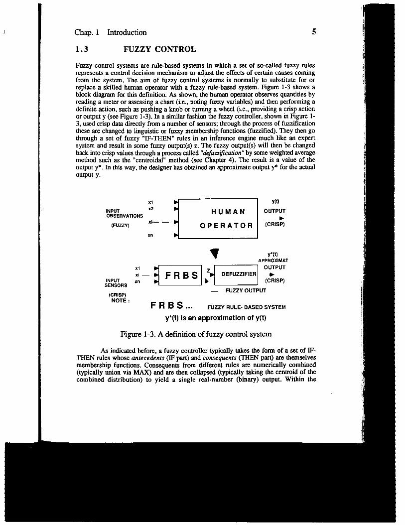
Fuzzy control systems are rule-based systems in which a set of so-called fuzzy rulesrepresents a control decision mechanism to adjust the effects of certain causes comingfrom the system. The aim of fuzzy control systems is normally to substitute for orreplace a skilled human operator with a fuzzy rule-based system. Figure 1-3 shows ablock diagram for this definition. As shown, the human operator observes quantities byreading a meter or assessing a chart (i.e., noting fuzzy variables) and then ~rforming adefinite action, such as pushing a knob or turning a whesl (i.e., providing a crisp actionor output y (see Figure 1-3). In a similar fashion the fuzzy controller, shown in Figure 1-3, used crisp data directly from a number of sensors; through the process of fuzzificationthese are changed to linguistic or fuzzy membership functions (fuzzified). They then gothrough a set of fuzzy “IF-THEN” rules in an inference engine much like an expertsystem and result in some fuzzy output(s) z. The fuzzy output(s) will then be changedback into crisp values through a process called “defuzzficatim” by some weighted averagemethod such as the “centroidal” method (see Chapter 4). The result is a vrdue of theoutput y*. In this way, the designer has obtained an approximate output y* for the actualoutput y.
INPUTOBSERVATIONS
(FUZZY)
::-*
INPUTSENSORS :-E
(CRISP)NOTE :
FRBS...
y(t)
OUTPUT
(CRIS?)
y*(t)APPROXIMATE
bel
OUTPUTDEFUZZIFIER
(C%ISP)
— FUZZY OUTPUT
FUZZY RULE- BASED SYSTEM
,1
,(
Figure 1-3. A definition of fuzzy control system 1’ii
As indicated before, a fuzzy controller typically takes the form of a set of IF-THEN rules whose untece&nts(IFpart) and cmsequents (THEN part) are themselves
?:
membership functions. Consequent from different rules are numerically combined(typically union via MAX) and are then collapsed (typically taking the centroid of the ~~combined distribution) to yield a single real-number (binary) output. Within the {

6 Chap. 1 Introduction
framework of a fuzzy expert system, like regular expert systems, typical rules can be theresult of a human opxator’s knowledge, e.g.:
“IF the Temperature is HotTHEN&crease the Current to a Medium level.”
In this rule, Hot and Medium are fuzzy variables. Such natural language rules can then betranslated into typical computer language statements such as :
IF(Ais Aland Bis Bland Cis Cland Dis Dl)THEN(Eis Eland Fis Fl)
Using a set of rules such as these, an entire finite number of rules can be derivedin the form of natural language statements as if a human operator were performing thecontrolling task. In any practical system, such as an air conditioning system, the user oran opxator often fine-tunes, tweaks, and adjusts the knobs until the desired cool (or hot)air can be felt with the desired speed. Such operator knowledge can be utilized in thedesign of a fuzzy controller form M conditioning unit system. One of the most commonways of designing a fuzzy controller is through “fuzzy rule-based systems.” Figure 14shows a typical fuzzy control architecture. The controller shows the prccesses offuzzification, (i.e., binary to fuzzy transformation) and defuzzification (i.e., fuzzy tobinary transformation).
System System OutputInput
, PLANT ++
● 1
1- SENSORI
II
I
InferenceEngine
Ct
WIesAeWianheinlfluflL
FUZZY CONTROLLER
Figure 1-4. Block diagram for a typical fuzzy control system showingfuzziiler (FUZZ), defuzzifier (DE-Fuzz), and inference engine.
An alternative way of implementing a fuzzy control regime, which is similar toa conventional adaptive control law, is to use a standard crisp logic controller such as, saya PID (u = Kp.e(t) + K int e(t)dt + Kd de(t)/dt), and then use fuzzy IF-THEN rules to“tune” the gains of the conventional controller, i.e., Kp Ki, and Kd. Here variable e(t) isthe tracking error for a system output y(t) which is to follow a desired output yd(t).Figure 1-5 shows one such adaptive fuzzy conirol architecture.
1.
TtenatmwaT(H(

Chain 1 Introduction 7
n . . I SYSTEM,, ~ ---.- ..-,
; = flx,u), y=g(x,u) -
x 1
CONTROLLER
u = h(e(t))
FUZZY LOGICADAPTATIONALGORITHM
f
Figure 1-5. An adaptive (self-tuning) fuzzy control system.
The fuzzy control problem, like any control problem, is one of evaluating amapping h(.), defined by
h : e -------------------> u
where u and e are the control and the error signals, respectively. The choice of h(.) is theessence of the control problem. For a two-sensor case, i.e., a two-error variable (say e andAe) and one control signal, the plot of u versus e and Ae will provide a surface this bookwill call control @we. Figure 1-6 shows two surfaces -- one (Figure l-6[a]) belongs toan expert controller and the other (Figure l-6~]) represents a fuzzy controller. As seenhere and indicated earlier, fizzy controllers are expert control systems that smoothlyinterpolate between crisp rules. This often results in a savings of energy, because thefuzzy control surface fits underneath the expert control surfacs. Chapters 4 and 5 will treatfuzzy control in some detail.
1.4 SCOPE OF THE BOOK
The basic theme of this book is fuzzy logic with software and hardware applications. Theentire book represents a result of teaching and resaeh on fuzzy logic and its applicationsat UNM’s CAD Laboratory for Intelligent and Robotic Systems for more than two years.The first six chapters represent an attempt to introduce readers to tlconcepts of fuzzy ~t.s, fuzzy logic, fuzzy control, and fuzzy software and hardware.Chapter 6 provides a brief overview of available fuzzy logic software. These softwarcs areTogai’s Fuzzy-C Systems, NeuraLogix’s NLX-230 Fuzzy Microcontroller, BellHelicopter Textron’s FULDEK, and UNM’s FLCG. At the end of the book is a postcard

8 Chap. 1 Introduction
that readers may use to obtain further information on the latter two mftware Pa&ages.Chapters 7 through 18 present various software and hardware projects which either havebeencompleted or were at a stage which initial results could be shared in open Wxature.
REFERENCES
1. Zadeh. L. A. (1%5). “Fuzzv Sets.” Information and Control. VOL8, PD. 335-353.

[ion
“es.
we:.
(a)
4r
Figure 1-6. Two control surfaces: (a) an expert control surface, and(b) a fuzzy control surface.
2
SET THEORY — CLASSICALAND FUZZY SETS
Timothy J. RossUniversity of New Mexico
2.1 INTRODUCTION
Fuzzy set theory is developed hereby comparing the precepts and operations of fuzzy setswith those of classical set theory. Fuzzy sets will be seen to contain the vast majority ofthe definitions, precepts, and axioms that define classical sets. In fact, very fewdifferences exist between the two set theories. Fuzzy set theory is actually afundamentally broader theory than current classical set theory, in that it considers aninfinite numlxr of “degrees of membership” in a set other than the canonical values of Oand 1 apparent in classical set theory. In this sense, one could argue that ctassicat sets area limited form of fuzzy sets. Hence, it will be shown that fuzzy set theory is acomprehensive set theory.
Conceptually, a fuzzy set can be defined as a collection of elements in a universeof information where the boundary of the set contained in the universe is ambiguous,vague, and otherwise fuzzy. It is instructive to introduce fuzzy sets by fwst reviewing theelements of classical (crisp) set theory.
10
2.
Dedisbeasin
XE
F,
A
A
A
x,Calem

‘s
o
tsofwa
Inorea
Chap. 2 Set Theory-Fuzzy and Crisp Sets 11
2.2 CLASSICAL SETS
Define X as the set of all objects with the same characteristics, called the universe ofdiscourse, whose individual elements are denoted by x. The elements of the universe canbe discrete and finite or continuous and infinite. Also, define the cardinality number, nx,as the total number of elements in X, A set A consists of collections of some elementsin X; set A is a subset of the universe X. Furthermore, the following notation holds:
x~ X --+x belongs to X
x~ A -+ x belongs to A
x= A + x does not belong to A
For sets A and B onX, we also have
AcB – A is contained inB
– VXE A, thenx~ B
A c B - A is fully contained in B
A=B – A~Band B~A
We define the null set, @, as the set containing no elements, and the whole set,X, as the set of all elements in the universe. All subsets of X comprise a special set
called the power set, P(X). For example, for the following universe X, the power set isenumerated
Example: We have a universe comprised of three elements, X = {a, b, c), so thecardinality is nx = 3. The power set is:
P(X)= {@, {a), {b), {c~, {a, b], (a, c), {b, c], {a, b,c)]
The cardinality of the power set, denoted rip(x), is found as:
Note that if the cardinality of the universe is infinite, then the cardinality of the power setis also equal to infinity, i.e., If nx = m + rip(x) = DO.
Operations on Classical Sets
Let A and B be two sets on the universe X. The union between the two sets, denotedAuB, represents all those elements in the universe which reside in (or belong to) eitherthe set A or the set B or both sets A and B. The intersection of the two sets, denotedAnB, represents all those elements in the universe X which reside in (or belong to) both .
sets A and B, simultaneously. The complement of a set A, denoted ~, is defined as the

12 Chap. 2 Set Theory-Fuzzy and Crisp Sets
collmion of all elements in the universe which do not reside in the set A. The differenceof a set A with respect to B, &%oted AU3, is defined as the collection of all elements inthe universe which reside in A and which do not reside in B simultaneously. Theseoperations are shown below.
Ct
- AuB=(xIx EAux=B)
Intersection; AnB=(xlx~A~x~B)
co mplemen~ ~={xlxe A,x EX]
Qif&QW2 AN3=(xlxe Aandx@B]
These four operations are shown below in terms of Venn diagrams in Figures 2-1 through
Figure+2-1. Union of sets A and B.
I
Figure 2-2. Intersection of sets A and B.

Chap. 2 Set Theory-Fuzzy artd Crisp Sets 13
Figure 2-3. Complement of set A.
Figure 2-4. Difference operation AN3.
Properties of Classical (Crisp) Sets.
Certain properties of sets are important to consider because of their influence on themathematical manipulation of sew. ‘l”hemost appropriate properties for purposes ofdefining classical sets, to show their similarity to fuzzy sets, anx
Commutativity: AuB = IIuAAnB = BnA
Assoeiativity: Au(BuC) = (AuB)~An(BnC) = (AW)nC
Distributivity: Au(BnC) = (AuB)n(A~)An(B@ = (-)u(Anc)
Idempotency AvA = AAnA=A
14 Chap. 2 Set Theory-Fuzzy and Crisp Sets
Identity AvO=AAnX=A
AnO= 0AuX = X
Transitivity: If AGBCC, Then ACC
Involution: ~=A
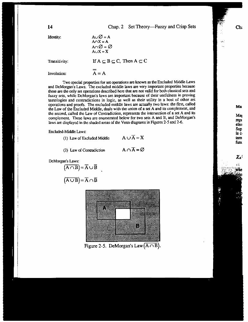
Two special properties for set operations are known as the Excluded Middle Lawsand DeMorgan’s Laws. The excluded middle laws are very important properties becausethese are the only set operations described here that are not valid for both classical sets andfuzzy sets, while DeMorgan’s laws are important because of their usefulness in provingtautologies and contradictions in logic, as well as their utility in a host of other setoperations and proofs. The excluded middle laws are actually two laws: the firsg calledthe Law of the Excluded Middle, deals with the union of a set A and its complement, andthe second, called the Law of Contradiction, represents the intersection of a set A and itscomplement. These laws are enumerated below for two sets A and B, and DeMorgan’slaws are displayed in the shaded areas of the Venn diagrams in Figures 2-5 and 245.
Exclude&Middle L.aws
(1) Law of Excluded Middle Au~=X
(2) Law of Contradiction An~=O
DeMorgan’s Laws:
(m).nJB .
Figure 2-5. DeMorgan’s Law (A n B).
.*,.

Chap. 2 Set Theory-Fuzzy and Crisp Sets 15
Figure 2-6. DeMorgan’s Law(A u B).
Mapping of Classical Sets to Functions

16 Chap.2 Set Theoxy-Fuzzy and Crisp Sets Ch.
And now the elements in the value set V(A) as determined ffom the mapping are,
WP(x)]=[(o, o,o,], (1,0,0], (0,1,0), (0,0, 1), {1, 1,0],{o, 1,1), ( 1,0, 1), {1, 1, 1]]
Now, define two sets on the universe X, sets A and B. The union of these two sets interms of function-theoretic terms is given by,
Union: AuB+ XAuB(X) = XA(X) v ~B(x)= lIIZiX&A(X), XB(X))
The intersection of these two sets in function-theoretic terms is given by,
Intersection: AnB + ~fiB(X) = ~A(X) A~B(X)= min(XA(x), XB(x))
The complement of a single set on universe X, say A, is given by,
Complement ~ ~ @x)= 1- CA(X)
For two sets on the same universe, say A and B, if one set (A) is contained in another set(B), then
Containment AGB+~A(X)<Z~(X).
2.3 FUZZY SETS
In classical sets, or crisp sets, the transition between membership and non-membership ina given set for an element in the universe is abrupt and well-defined (said to be “crisp”).For an element in a universe which contains fuzzy sets this transition can be gradual.This transition among various degrees of membership can be thought of as conforming tothe fact that the boundaries of the fuzzy sets are vague and ambiguous. Hence,membership of an element from the universe in this set is measured by a function whichattempts to describe vagueness and ambiguity.
A fuzzy set then is a set containing elements which have varying degrees ofmembership in the set. This idea is contrasted with classical, or crisp, sets becausemembers of a crisp set would not be members unless their membership was full or
m complete in that set (i.e., their membership is assigned a value of 1). Elements in afuzzy set, because their membership can be a value other than complete, can also bemembers of other fuzzy sets on the same universe.
Elements of a fuzzy set are mapped to a universe of “membership values” usinga function-thwxetic form. Fuzzy sets are denoted by a set symbol with a tilde understrike;so for example, A would be the “fuzzy set” A. This function maps elements of a fuzzy
Iset
x, i!
The

jets
set
J“).Ml.;toIce,~ich
: ofuseor
nabe
ingke;Zzy
Chap. 2 Set Theory-Fuzzy and Crisp Sets 17
set A to a real numlx.redvalue on the interval Oto 1. If an element in the universe, say
x, is a member of fuzzy set A then this mapping is given as,
PA(X) E [W]
A = (X,/fA(X)lX E X)
These mappings are shown below in Figures 2-7 and 2-8 for crisp and fuzzy sets,respectively.
1
n-
0K
Figure 2-7. Membership function for crisp set A.
1
n’
o
A
L x
Figure 2-8. Membership function for fuzzy set A.
A notation convention for fuzzy sets that is popular in the literature when theuniverse of discourse, X, is discrete and finite, is given below for a fuzzy set A by,
* /f A(xI) /4A(x2)
x
/f A(xi)=- + - +“.”””””””””””””= -
xl X2 i Xi
and, when the universe, X, is continuous and infinite, the fuzzy set A is denoted by,
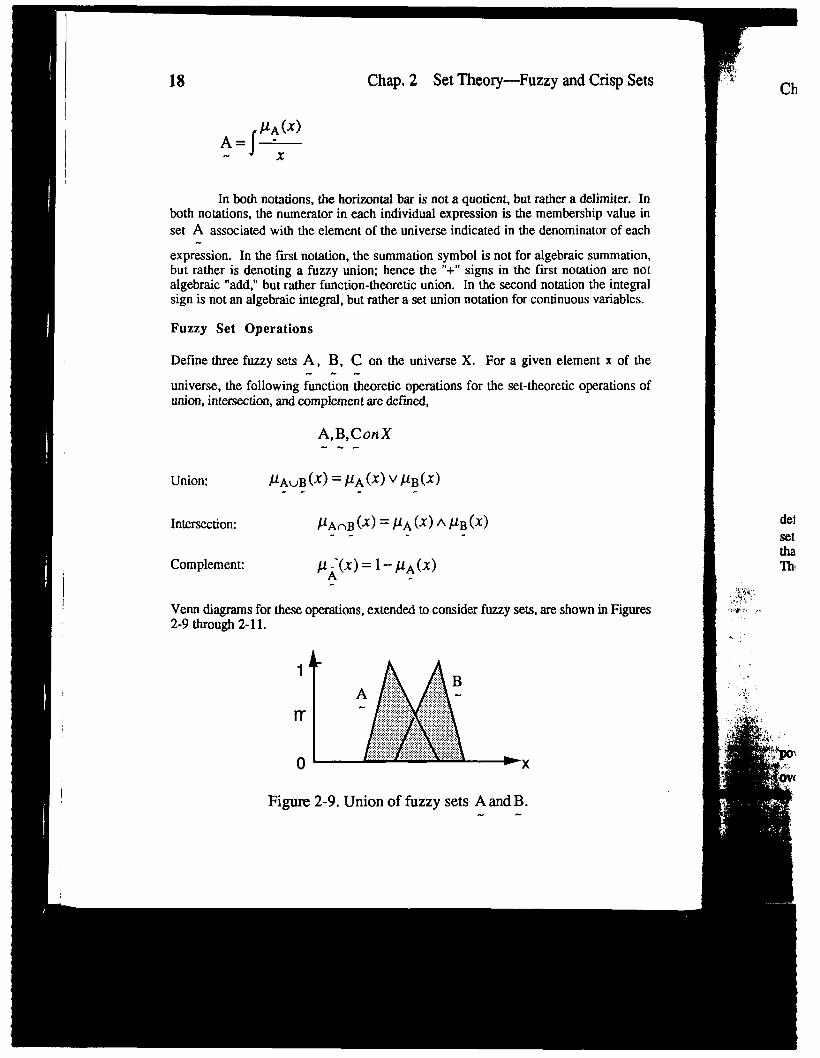
PA(X)A=j-
X
In both notations, the horizontal bar is not a quotient, but rather a delimiter. Inboth notations, the numerator in each individual expression is the membership value inset A associated with the element of the universe indicated in the denominator of each
expression. In the f~st notation, the summation symbol is not for algebraic summation,but rather is denoting a fuzzy union; hence the “+” signs in the first notation are notalgebraic “add,” but rather function-theoretic union. In the second notation the integralsign is not an algebraic integral, but rather a set union notation for continuous variables.
Fuzzy Set Operations
Define three fuzzy sets A, B, C on the universe X. For a given element x of the---
universe, the following function theoretic operations for the set-theoretic operations ofunion, intersection, and complement are defined,
A, B,ConX--
Intersmtion: )JAnB@) = PA(X) A ~B(x)-- -
Complement PA(X) = 1‘/fA(X)
Venn diagmrns for these operations, extended to consider fkzzy sets, are shown in Figures2-9 through 2-11.
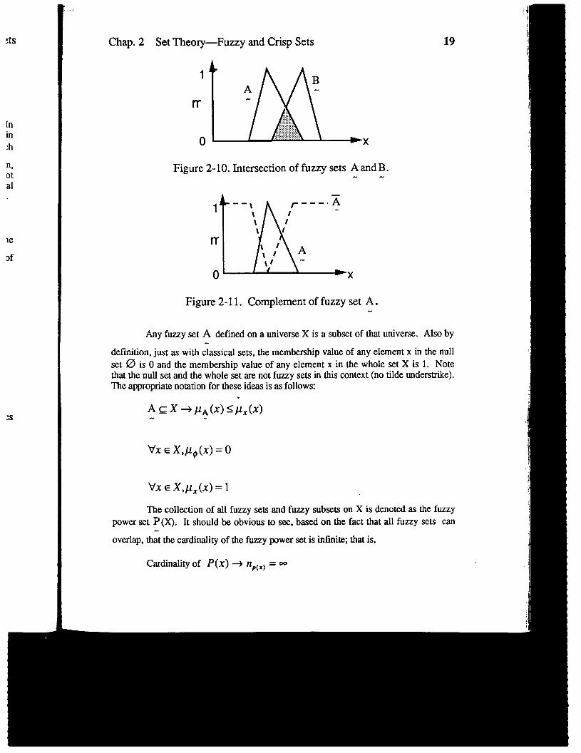
Figure 2-9. Union of fuzzy sets A and B.
:ts 19
[nin:h
n,Otal
1
n-
o
1
r-r
c
2s

11 DeMorgan’s laws for classical sets also hold for fuzzy sets, as denoted by theexpressions below,
II [AnB] = AuB
()AuB =~n B--- -
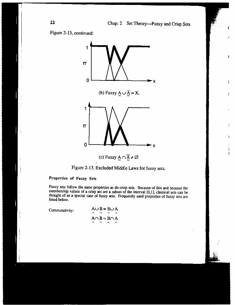
All other operations on classical sets, as enumerated before, also hold for fuzzysets, except for the excluded middle laws. These two laws do not hold for fuzzy setsbecause of the fact that since fuzzy sets can overlap, a set and its complement can alsooverlap. The excluded middle laws, extended for fuzzy ws, are expressed by,
Auh X
I AnA##
I.-
1 Extended Venn diagrams for these situations, and comparisons to the excludedmiddle laws for classical (crisp) sets, are shown below in Figures 2-12 and 2-13.
I
I
. LA A
r-f
o x
(a) Crisp set A and its complement.
Figure 2-12. Excluded Middle Laws for crisp sets.

~Sets
y the
‘Uzzy‘ setsalso
uded
I
Chap. 2 Set Theory-Fuzzy and Crisp Sets
Figure 2-12, continued:
:Lx(b) Crisp Au~ = X.
1
m
I
(c)Crisp An~ = 0.
Figure 2-12. Excluded Middle Laws for crisp sets.
1’
‘r-f
o
,-- \\\\
(a) Fuzzy set ~ and its complement.
Figure 2-13. Excluded Middle Laws for fuzzy sets.
21
I
22 Chap. 2 Set Theo~-Fuzzy and Crisp Sets
Figure 2-13, continued:
f-r
o
1
IY
o
(c) Fuzzy ~ n ~ # 0.
Figure 2-13. Excluded Middle Laws for fuzzy sets.
Properties of Fuzzy Sets
Fuzzy sets follow the same properties as do crisp sets. Because of this and because themembership values of a crisp set are a subset of the interval [0,1], classical sets can bethought of as a special case of fuzzy sets. Frequently used properties of fuzzy sets arelisted below.
1
1
i!
Commutativity: Au B=Bu A--- -
An B=Bn A--- -
ts Chap. 2 Set Theo~-Fuzzy and Crisp Sets 23
kociativity:
W“:)=($’4u:and+9=@’W
Distributivity:
- (--) (--) (- .-) - (--) (--)(--)Au BnC = AuB m AuC andAn BuC = AnB u AnB
Idempotency Au A= AandAn A=A--- ---
Identity:AU O= Aand AnX=A andAn O= OandAu X=X
Transitivity: ~A~B~C,thenACC--- .-
Involution: ~=A--
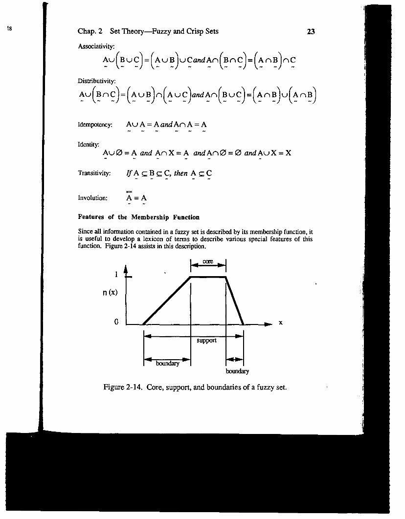
Features of the Membership Function
Since all information contained in a fuzzy set is described by its membership function, itis useful to develop a lexicon of terms to describe various special features of thisfunction. Figure 2-14 assists in this description.
1
n (x)
o
F-1.●
x
Figure 2-14.
tmndary
Core, support, artd boundaries of a fuzzy set.

24 Chap.2 Set Theory-Fuzzy and Crisp Sets
The core of a membership function for some fuzzy set A is defined as that
region of the universe that is characterized by complete and full membership in the setA. That is, the core is comprised of those elements of the universe, x, where P.A (x)=
1.
The support of a membership function for some fuzzy set A is defined as that
region of the universe that is characterized by non-zero membership in the set A. That
is, the support is comprised of those elements of the universe, x, where p A(x) #O.
The boundaries of a membership function for some fuzzy set A are defined as
that region of the universe that contains elements that have a non-zero membership, butnot complete membership. That is, the boundaries are comprised of those elements of theuniverse, x, where 0< v A (X) <1. These elements of the universe are those with some
“degree” of fuzziness, or only partial membership in the fuzzy set A. Figure 2-14
illustrates the regions in the universe comprising the core, support, and boundaries of atypical fuzzy set.
A normal fuzzy set is one whose membership function has at least one elementin the universe, x, whose membership value is unity. For fuzzy sets where one and onlyone element has a membership LX@ to one, this element is typically referred to as the
&
ChaI.’
momincrethe u
y<z
then
and i
A
L
1
I-f
x o
.
Figure 2-15. Normal (left) and non-normal (right) fuzzy sets.
A convex fuzzv set is described by a membership function whose membership

Chap,2 Set Theo~-Fuzzy and Crisp Sets 25
monotonically decreasing, or whose membership values are strictly monotonicallyincreasingthen strictly monotonicallydecreasingwith increasingvalues for elements inthe universe. Said anotherway, if for all elements in a continuous fumy set A wherex <
y c z, and where
/-LA(Y) ~miI@A@)~~A(z)l.
then A is said to be a convex fuzzy set. Figure 2-16 shows a typical convex fuzzy set
and atypical non-convex fuzzy set,
L Ai
Figure 2-16. Convex fuzzy set (top) and non-convex fuzzy set (bottom).
It should be noted, that a special property of two convex fuzzy sets, say A and
B, is that the intersection of these two convex fuzzy sets is also a convex fuzzy set, as
shown in Figure 2-17. That is, for A and B, which are both convex, An Bis also.-
convex.

26
1
IT(x)
(
I
Chap.2 Set Theory-Fuzzy mdCrisp Sets
A
-x
Figure 2-17. The intersection of two convex fuzzy sets.
Extension Principle
Heretofore we have discussed features of fuzzy sets on certain universes of discourse.Suppose there is a mapping between elements, u, of one universe, U, onto elernenWv,of another universe, V, through a function f. An extension principle developed by Zadeh(1975) and later elaborated by Yager (1986) allows us to extend the domain of a functionon fuzzy sets. Let this mapping be descti~ by,
Let fiu+v
Define A to be a fuzzy set on universe U; that is, A c U, and
A=~+a+............hU1 lq Un
Then the extension principle asserts that, for a function f that maps one element inuniverse U to one element in u’tiverse V,
= lfl:/f2:f(A) f( +P............. —% U2
U*)
=P1P2: + k. . . . . . . . . . . . —
f(%) + f(%) f (u*)
This mapping is said to be “one-toae.”
Example:Leta fuzzy set A be defined on the universe U = {1, 2, 3). We wish to
map elements of this fuzzy set to another universe, V, under the function
v= f(u) =2u-1.
WtCain’ismfuth(

Chap.2 Set Theory-Fuzzy and Crisp Sets 27
Weseethat theelements of Vare, V={l,3,5). So, forexample suppose the fuzzyset A is given by,
;= 0.6+1+0.8—— —1 2 3’
then the fuzzy membership function for v = f(u),= 2u-1 would be,
f(A) = 0.6+1+0.8—. —1?5
Urse.
ts,v,adehXion
It in
=lto
For cases where this functional mapping f maps products of elements from two universes,say U1 and U2, to another universe V, and we define A as a fuzzy set on the Cartesian
space U1XU2, then
f(A)={_l\i~ul,j~%}
where p 1(i) and p2Q) are the separable membership projections of ~(ij) from theCartesian space U1 x U2 when p(i j) can not be determined. This projection involves theinvocation of a condition known as “non-interaction” between the separate universes, andis analogous to the assumption of independence employed in probability thexxy whichreduces a joint probability density function to the product of its separate marginal densityfunctions. In the fuzzy non-interaction case we use the minimum function as opposed tothe product function used in probability theory.
Example: Suppose we have the integers 1 to 10 as the elements of two identicalbut different universes; la
U1 =U2= (1,2,3, ...... 10], then define two fuzzy sets A and B on universe
U1 and U2, respectively,
o.6+l+o.8tiRfine A = 2 =“ approximately 2“= — – —.-
O.;+ 12+0.;defm B = 6 =“ approximately 6’= — – —-- 5 6 7’
then the product of (“approximately 2“) x (“approximately 6) should map to a fuzzynumber “approximately 12,” which is a fuzzy set defined on a universe, say V, ofintegers, V=(5, 6, ..... 18, 21), as determined by the extension principle,

28 Chap.2 Set Theory-Fuzzy artd Crisp Sets
(
0.6+ 1 +0.8
)(
0.8 + 1 + 0.72x6=—–——–—.- 1 23X 567 )
= min(O.6,0.8)+ min(O.6,1) + + min(O.8,1) + min(O.8,0.7)
5 6.. ... ... ...
18 21
= 0.6+ 0.6+0.6 +0.8 +~+0.7 +0.8+0.8+0.7——TTY ti12ti =1821
The complexity of the extension principle increases when we consider if morethan the combination of the input variables, UI and U2, are mapped to the same variablein the output space, V. In this case we take the maximum membership grades of thecombinations mapping to the same output variable, or for the mapping shown below weget,
/h(U@’2) = ‘w[tin{/@l)#2(k!)}]
I >ExamDie: We have two fuzzv sets a and b. each defined on its own universe, as
I We wish to determine the membership values for the mapping
~a, b)=axb “--- -
= min(O.2, 0.5) + max[min(0.2,1), min(O.5,1)] + max[min(0.7,0. 5),min(l, 1)] + min(O. 7, 1)
1 2 4 8
I -+-‘—+7_+4 81
In this case, the mapping involves two ways to produce a 2 (1x2 and 2x1) and twoways to produce a 4 (4x1 and 2x2).
2.4 RELATIONS AMONG CLASSICAL (CRISP) SETS
The Cartesian product of two univexses X and Y is determined as

,...
Chap. 2 Set Theory-Fuzzy and Crisp Sets 29
xkY={(x,y)/x ex,y EY}
which combines Vx ● X and Vy G Y in an ordered pair and forms ~nco nstrainedmatches between x and y. That is, every element in universe X is related completely toevery element in universe Y. The “strength” of this relationship behveen ordered pairs ofelements in each universe is measured by the characteristic function, where a value ofunity is associated with “complete relationship” and a value of zero is associated with “norelationship,” i.e., the binary values 1 and O. An example is given in the Sagittaldiagram shown below, and in the matrix expression to follow, where values of unity inthe relation marnx, denoted R, correspond to the ordered pairs of mappings in the relation.
xi Y
●
●
abc
1
2
3
Figure 2-18. Sagittal diagrams (top) and matrix expressions (bottom)of an unconstrained relation.
A more general crisp relation, R, exists when matches between elements in two I
universes are constrained. Again, the characteristic function is used to assign values ofrelationship in the mapping of the Cartesian space X x Y to the binary values of (0,1).
E-wmple: In many biological models, members of certain species can reproduce onlywith certain members of another species. Hence, only some elements in two ormore univer~ are paired. An ex~ple is shown below for two 2-member species.

ab
R = {(La),(2,b)} RcXXY [1110R=
201
0000
0000
0000
0000
E=
1111
1111
1111
1111
now be detined. - .
Union: R u S + ~RuS(x,y) = max[~R(x, y),~S(x, y)]
Intersection: R nS + XR~~(x,y) = rnin[~R(x,y),~~ (x,y)]
Complemerm R+z~(x,Y) =l-zR(x!Y)
Containment R C~ + ~~(X,y) <~~(X,y)
Identity (O+ OamiX + E)
Further, the operations of commutativity, associativity, distributivity,involution, and idempotency all hold just as they do for classical set operations.Moreover, DeMorgan’s laws and the Excluded Middle laws also hold for crisp (classical)
C
nm
uuFd2
(

Chap. 2 Set Theory-Fuzzy and Crisp Sets 31
relations just as they do for crisp (classical) sets. The null relation, O, and the completerelation, E, are analogous to the nuU set and the whole set in set-theoretic form.
Now let R be a relation that relates, or maps, elements from universe X touniverse Y, and let S be a relation that relates, or maps, elements from universe Y touniverse Z. Can we find a relation, T, that relates the same elements in universe X thatR handles to the same elements in universe Z that S handles? The answer is yes, and wedo this with an operation known as ~. So for the Sagittal diagram in Figure2-19, we wish to find a relation T that relates the ordered pair (Xl, Z2); i.e.,
(x~,z+r
5
X2
%
x Y z
‘1
\
‘2.
‘3 .
‘4
z
?2
Figure 2-19. Sagittal diagram relating elements of three universes.
There are two common forms of the composition operation; one is called themax-min composition and the other is termed the max-product composition. The max-min composition is defined by the-expression
T=Ro S
~T(X,Z) = ~#~R(X,y) A ~~(y, Z))
and the max-product (sometimes called mix-dot) composition is defined by theexpression,
T=Ro S
%T(x,z) = V#x, y) “x~(y,z))
Exumpie: The matrix expression for the crisp relations shown in Figure 2-19 canbe found using the max-rnin composition operation. Relations R and S would beexpressd as,

32 Chap.2 Set Theory-Fuzzy artd Crisp Sets
YI Y2 Y3 Y4 % Z2
The resulting relation T would then be determined by max-min composition as,
z, Z2
[1X,ol
T=x200
X300
2-5 RELATIONS AMONG FUZZY SETS
Fuzzy relations also map elements of one universe, say X, to those of another universe,say Y, through the Cartesian product of the two universes. However, the “strength” ofthe relation between ordered pairs of the two universes is not measured with thecharacteristic function, but rather with a membership function expressing various“degrees” of the strength of the relation on the unit interval [0,1]. Hence, a fuzzy relationR, is a mapping from the Cartesian space X x Y to the interval [0,1], where the strength
of the mapping is expressed by the membership function of the relation for ordered pairsfiOm he tWO UIIiVeH&3, or w R(?.y).
Cardinality of Fuzzy Relations
Since the cardinality of fuzzy sets on any universe is infinity, then the cardinality of afuzzy relation LxXweentwo or more universes is also infinity.
Operations on Fuzzy Relations
Let R, S, and T be fuzzy relations on the Cartesian space X x Y. Then the following.-
operations apply,
Union: ~Ru@’) = ‘n(~R(X,Y)#S(X$Y))

.,
iii’
Chap.2 Set Theory-Fuzzy and Crisp Sets 33
Intersection: ~Rr&,Y) = fi@R(~!Y)~~s(X3Y))--
Complementi @Y) = l-~R(X,Y)-
Containmerm R C S =~R(x,y) </f~(X,y).- .
Just as for crisp relations, the operations of commutativity, associativity,distributivity, involution, and idempotency all hold for fuzzy relations. Moreover,DeMorgan’s laws hold for fuzzy relations just as they do for crisp (classical) relations, andthe null relation, O, and the complete relation, E, are analogous to the null set and thewhole set in set-theoretic form, respectively. The operations that do not hold for fuzzyrelations, as is the case for fuzzy sets in general, are the Excluded Middle laws. Since afuzzy relation R is also a fuzzy set, there is overlap between a relation and its
complemen~ and
Ru~#E--
Rn~#O--
As seen, the Excluded Middle laws for relations do not result in the null relation, O, orthe complete relation, E.
Because fuzzy relations in general are fuzzy sets, we can define the Cartesian
product between fuzzy sets. W ~ be a fuzzy set on universe X and B be a fuzzy set on
universe Y, then the Cartesian product between fuzzy sets A and B will result in a fuzzy
relation R, or
AxB=R c XXY-., -
with membershipfunction,
/f@ = /hx)3(x$)’) = m+A(x)Yk(y))-.

34 Chap. 2 Set Theory-Fuzzy and Crisp Sets
Example: Suppose we have two fuzzy sets on a universe, A and B , and we want
to find the fuzzy Carte&n product between them. L@
A _ 0.2 +0.5+1—_ __ and B = ~+~% Xz X3 Y1 Y2
Then the fuzzy Cartesian product is,
% Z2
xl [0.2 0.21
HAxB=R= X2 0.3 0.5---
X3 0.3 0.9
FQ
. .
,. Ch;i:...~,
~
. ... ‘.“
,*’,., ,,..-
in:
Fuzzy composition can be defined just as it is for crisp (binary) relations.
Suppose R is a fuzzy relation on the Cartesian space X x Y, S is a fuzzy relation on Y
x Z, and T is a fuzzy relation on X x Z; then the fuzzy max-min composition is defined
as:
Let T=Ro S---
ThCOI~.
RI
Ya
Za
and the fuzzy max-product composition is defined as,
MT(LZ)= v (/.@3Y) ● PS(YA)yd’ -
Exumple: Letusextend the information contained in the Sagittal diagram shown inFigure 2-19 to include fuzzy relationships between the universes X-Y (denoted bythe fuzzy relation R) and Y-Z (denoted by the fuzzy relation S). Consider the
following fuzzy relations,

:ts
=
nt
‘s.
Y
xl
Chap. 2 Set Theory-Fuzzy and Crisp Sets 35
Then the resulting relation, T, which relates elements of univeme X to elements of
universe Z, ean be found by max-min composition to be,
-[
0.7 0.6 0.5T=
0.8 0.6 0.41It should be pointed out that neither crisp nor fuzzy compositions have inverses
in general; that is
RoS+SOR
--- -
This remdt is general for any matix o~ration, fuzzy or otherwise, which must satisfyconsistency between the cardinal counts of elements in respective universes. Even for thecase of square matrices, the composition inverse is not guaranteed.
REFERENCES
Yager, R. R. (1986) “A chwteri~hon of the extension principle,” Fuzzy Sets andSystems, 18, 205-217.
Zadeh, L. A. (197S) “The concept of a linguistic variable and its application toapproximate reasoning,” Information Sciences, 8, 199-249; and also 9,43-80.
‘Yie

3
PROPOSITIONALCALCULUS — PREDICATELOGIC AND FUZZY LOGIC
Timothy J. RossUniversity of New Mexico
.
3.1 PREDICATE LOGIC
In classical predicate logic, a simple proposition, P, is a linguistic statement containedwithin a universe of mmositions which can be identified as being strictly true or strictly
value of 1 (truth) or O (false). If U is the universe of all propositions, then T is amapping of these propositions to the binary quantities (O, 1), or
T: U + {0,1}
Now let P and Q be two simple propositions on the same universe of discourse .that can be combimx! using the foUowing five logical connective,
36
*+.,:.,:. “,,
. .
Ct
(i)
(ii)~..i
(iv
(v)
toCa
linprisse
)
!d[ye,tsaa
Chap. 3 Predicate Logic and Fuzzy Logic 37
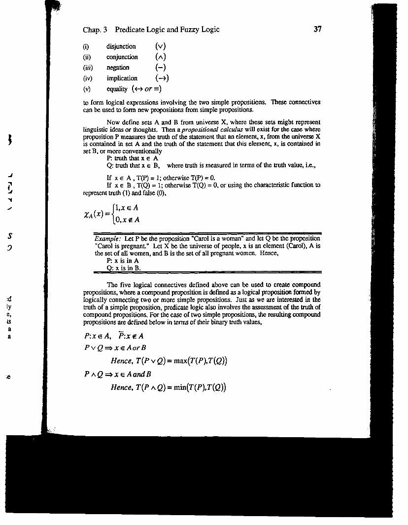
(i) disjunction (v)
(ii) conjunction (A)
(iii) negation (-)
(iv) implication (+)
(v) U@@ (e or =)
to form logical expressions involving the two simple propositions. These connectivecan be used to form new propositions from simple propositions.
Now define sets A and B from universe X, where these sets might representlinguistic ideas or thoughts. Then a propositional calculw will exist for the case whereproposition P measures the truth of the statement that an element, x, from the universe Xis contained in set A and the truth of the statement that this element, x, is eonrained inset B, or more conventionally
Ptruththatxe AQtruththatx EB, where truth is measured in terms of the truth value, i.e.,
If x ~ A, T(P)= 1; otherwise= O.If x e B , T(Q = 1; otherwise T(Q)= O,or using the characteristic function to
represent truth (1) and false (0),
{
1,x G A2A(X) =
O,x @A
Example: LetP be the proposition “Carol is a woman” and let Q be the prcymsition“Carol is pregnan~” Let X be the universe of people, x is an element (Carol),A isthe set of all women,and B is the set of dl pregnantwomen. Hence,
Pxis inAQ: x is in B.
The five logical connective defined above can be used to create compoundpropositions, where a compound proposition is defined as a logical proposition famed bylogically connecting two or more simple propositions. Just as we are interested in thetruth of a simple proposition, predieate logic also involves the assessmentof the truth ofcompound propositions. For the case of two simple propositions, the resulting compoundpropositions are &fmed Mow in terms of their binary truth values,
PxEA, ~:xe/i
PvQax~AorB
Hence, T(P v Q) = max(T(P),T(Q))
PAQ~x~AandB
Hence, T(P A Q) = min(T(P),T(Q))

38 Chap. 3 Predicate Logic and Fuzzy Logic
lfT(P) = 1, then T(P)=& ljT(P) = O, then T(7)= 1
P- Q~x EA,B
Hence, T(P e Q) = T(P)
= T(Q)
The logical connective “implication” presented here is also known as theclassical implication, to distinguish it from an alternative form due to Lukasiewicz, aPolish mathematician in the 1930s, who was first credited with exploring logics otherthan Aristotelian (classical or binary logic) logic. This classical form of the implicationoperation requires some explanation.
For a proposition P defined on set A and a proposition Q defined on set B, theimplication “P implies Q“ is equivalent to taking the union of elements in thecomplement of set A with the elements in the set B. That is, the logical implication isanalogous to the set-theoretic form,
Chq
tluth ‘Thes(
below
P
P + Q E ~vBistrue E either “notinA’’or’’inB”
xl)
ql)
F(O)
F(O)
Pis:
impliby
Sothat(P+Q)-(~v Q)
T(P + Q) = T(Pv Q) = max(T(~),T(Q))
This is linguistically equivalent to the statement, “P implies Q is true” wheneither “not A“ or “B” is true. Graphically this implication and the analogous setoperation is represented by the Venn diagram in Figure 3-1. As noted in the diagram, theregion represented by the difference A/El is the set region where the implication “Pimplies Q“ is false (the implication “fails”). The shaded region in Figure 3-1 representsthe colketion of elements in the universe where the implication is true.
The shaded area is the sec
()A\ B=~u B= ~
IfxisinAandxisnotinBthen
A + B fails= A / B(difference)

)gic
the:sh;ion
thethelis
lensetthe“Pnts
‘)
!!&?,
ii.
Chap. 3 Predicate Logic and Fuzzy Logic 39
Now, with two propositions (P and Q) each being able to take on one of two
truth values (true or false, 1 or O), there will be a total of 22 = 4 propositional situations.These situations are illustrated, along with the appropriate truth values, for thepropositions P and Q and the various logical connective between them in the truth tablebelow.
P Q F PvQ PAQ P+Q P+Q
T(1) T(1) F(0) T(1) T(1) T(1) T(1)
T(1) F(0) F(0) T(1) F(0) F(0) F(0)
F(0) T(1) T(1) T(1) F(0) T(1) F(0)
F(0) F(0) T(1) F(0) F(0) T(1) T(1)
Suppose the implication operation involves two different universes of discourse;P is a proposition described by set A, which is defined on universe X, and Q is aproposition described by set B, which is defined on universe Y. Then the implication “Pimplies Q“ can be represented in set-thearetic terms by the relation R, where R is definedby
R =(AxB)u(AxY) = IFA, THEN B
Ifx EA where x ● X,A c X
thenyc B where y~Y, BcY
This implication is also equivalent to the linguistic rule form: IF A, THEN B.The graphic shown below in Figure 3-2 represents the Cartesian space of the product X xY, showing typical sets A and B, and superposed on this space is the set-theoreticequivalent of the implication. That is,
P+ Q~Ifx~A, thenre B,or P+ Qs~UB
I
.;.:;.:;.:::,:?W:./:.::!?*{::I:.\;,............c......’.. ./,,,.,..,.,,,,,.,,:.>:.......%W.?..%....x.,.,....x.,.............:<.+<.:.:<.T?,!i::::~,;.;..,;}.:,:,:,;,;A
:i.::::fiz.:+:..\..%.,.,..,.),~:,:,:,:,:................,..,,,.,.},.,.,,,,,,,............. .,..,,.,...,,.}.,.,~.t,:.,.,.,..............
B
Figure 3-2. The Cartesian space showing the implication IF A, THEN B.
.,

40 Chap. 3 Predicate Logic and Fuzzy Logic
The shaded regions of the compound Venn diagram in Figure 3-2 represent the truthdomainof the implkation, IF A, THEN B (P impliesQ).
Anothercompoundpropositionin linguisticrule form is the expression,
IF A, THEN B, ELSE C.
In predieate logic this has the form,
(P+ Q)v(%S)
where P:xc A,Ac X
Qy-B,Bc Y
s:y Ec,cc Y
Linguistkzdly,this compoundpropositioncouldbe expressedas,
IF A, THEN B, or
~ I, THENC.
The set-theoreticequivalentof this compoundpropositionis givenby,
IF ATHENBEIJjEC S(AXB)U(-M)= R=relationonXx Y
The graphic shown in Figure 3-3 illustrates the shaded region representing thetruth domain for this compound proposition.
YJ ‘ _:.:.:,:.:.::::::.:,:::::.~,~~.:,:,:.:.,,,.,.,,,.,.,.:,:,: ..’.‘..’.,,,$.]:.’.:,:.:.:,:::::::::.:::::::.:,:,~.:.;,;.:.;,;~{.:.:.:.:.,}.:.:.:.:.:.::.:.:......................,,,,.,.,.....fi:y::~:j:~; ;,Y,%::t.:;::,:,:,~:::::!.:;,:.:,~::::::;.:.::~,i:.,,,.,.,,,.,.,,..,.,:, .......,*..,..,,,,..,..,..................... ..................................................................................... .............:.:.:.:.:.:.:.:.:.:.:.::::::~::::::::::::::,,:,:,:,:,:
...,,,,.,m:::::;::;fij:j:;::::,::::::j::::,, .............. .,.,,. ,.,::::~fi:::*,:: ;,$:~,x:;.........................................................A
;:~:,:,:,,,,.,.,.,,,.,,,,,,,:.:.:.:.,.:,:.>:.=,::,............,...................:.:.:.:.:.:.:.:,:::::::::~~::;\+,;:*:::.:!.X:::,:::::,.::,,.:...,.,,......,,,.,,.,,,.,,g##@g~;$~,.:.:,:.:.:,:.:.:,:.:.:,:.,.:,:.:.:,:.:.:,:.:.,.,.:.:.:.,.::,:::::,:::::::::::::,:=,,;.~.~.~i:.,.,.,,,.,.,,,.,.,,,.,..:,::::::::::fii:j~j{~,~:::,:kz.:<.k.;....................................,.,,,.,,,,.,..,:::,:,:%,:,::.:.X:::,:.:.:,..:::,:.,................................+-v.....+?X,:,:,:,.,,:=:.:.’.:.,.:,:,::,::,:,:::,:,:,:,:<::,:,.....-.~.....,x<.x,.:?.::::,:~.:::.,.:.:.,.:~~:=::w: ,,.,.:.,,,.:.:,,.:.,,x..........
B c
Figure 3-3. Truth domain for IF A THEN B ELSE C.

;ic
Jth
he
Chap. 3 Predicate Logic and Fuzzy Logic 41
Tautologies
In predicate logic it is useful to consider compound propositions that are always true,irrespective of the truth values of the individual simple propositions. Classical logicalcompound propositions with this property are called “tautologies.” Tautologies are usefulfor deductive reasoning and for making deductive inferences, So, if a compoundproposition can be expressed in the form of a tautology, the truth value of that compoundproposition is known to be true. Inference schemes in expert systems often employtautologies. The reason for this is that tautologies are logical formulas that are true onlogical grounds alone.
One of these, known as Modus Ponens deduction, is a very common inferencescheme used in forward chaining rule-based expert systems. It is an operation whose taskis to find the truth value of a consequent in a production rule, given the truth value of theantecedent in the rule. Modus Ponens deduction concludes that, given two propositions, aand a-implies-b, both of which are hue, then the truth of the simple proposition b isautomatically inferred. Another useful tautology is the Modus Tollens inference, whichis used in backwarddaining expert systems. In Modus Tollens an implication betweentwo propositions is combined with a second proposition and both are used to imply athird proposition. Some common tautologies are listed below.
~uB-X (AA (A+ B)) + B (Modus Ponens)
AuX; Ku X*x (~A(A + B)) + ~(Modus Tollens)
A proof of the truth value of the Modus Ponens deduction is listed here.
Proofi (AA(A + B))+ B
(A@JB))+B
((AA~)u(AA+B
(W(AAB))+B
(A AB)+B
(-)UB
(WUB

42 Chap. 3 Predicate Logic and Fuzzy Logic
b(~uB)
Kux
X+ T(X)=l; QlZ!2
A similar display of the truth value of this tautology is shown below in ~th table form.
A B A+B (&lA+B)) (&(A+B))+B
.-
Asir
A
0
0
1
1
Coni
Com~indiwconw,
Dedu
The Ntypiea
Bu(Au~)

ic
44 Chap.3 Predicate Logic and Fuzzy Logic
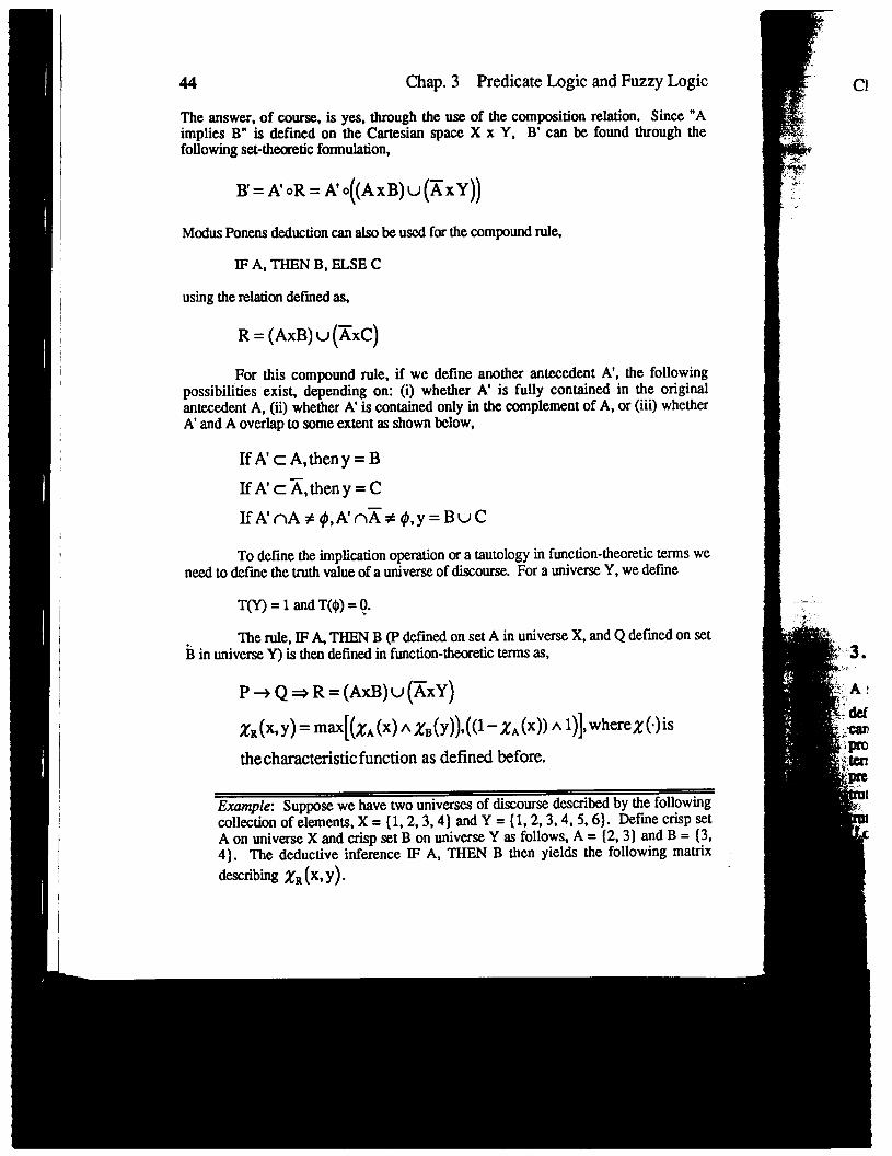
The answer, of course, is yes, through the use of the composition relation. Since “Aimplies B“ is defined on the Cartesian space X x Y, B’ can be found through thefollowing sel-theoretic fonnu.lation,
B’=A’oR=A’o((AxB) u(~xY))
Modus Ponens deduction can also be used for the compound rule,
IF A, THEN B, ELSEC
using the relation defined as,
R= (AxB) U (XXC)
For this compound rule, if we define another antecedent A, the followingpossibilities exist, depending on: (i) whether A’ is fully contained in the originalantecedent A, (ii) whether A’ is contained only in the complement of A, or (iii) whetherA and A overlap to some extent as shown below,
If A’c A,theny=B
If A’c X,theny=C
If A’nA#&A’n~#$,y=Bu C
To define the implication operation or a tautology in function-theoretic terms weneed to define the truth value of a universe of discourse. For a universe Y, we define
T(Y) = 1 and T($)= O.
The rule, IF L THEN B (P defined on set A in universe X, and Q defined on setBin universe Y) is then defined in function-theoretic terms as,
P+ Q~R=(AxB)u(~xY)
ZR(xJY) = ‘m[(~A (x) A 2B(Y)),((1 ‘%A(X)) A l)],where~(.)is
thecharacteristic function as defined before.
Exumple:Suppose we have two universes of discourse described by the followingcollection of elements, X = (1, 2,3,4) and Y = (1, 2,3,4, 5, 6). Define crisp setA on universe X and crisp set B on universe Y as follows, A = (2,3) and B = (3,4]. The deductive inference IF A, THEN B then yields the following matrix
describing ~R(X,Y).

Chap.3 Predicate Logic and Fuzzy bgic
123456
[i
1111111
2001100R=
3001100
4111111
45
The compound rule IF A, THEN B, ELSE C is defined as
R=(AxB)u(AxC) +(P+Q)V(~+S) andwehave
X,(X3Y) = rnax[(x.(~) A2’B(Y)),((l -X.(x)] A XC(Y))]
Example: Continuing with the previous example, suppose we define a crisp set Con universe Y as C = (6, 7). The deductive inference IF A THEN B ELSE C then
yields the following matrix describing ~~ (x, y).
123456
lPoooll-2 001100
R=3 00110041000011,
3.2 FUZZY LOGIC
A fuzzy logic preposition, P, is a statement involving some concept without clearly
defined boundaries. Linguistic statements that tend to express subjective ideas and whichcan be interpreted slightly differently by various individuals typically involve fuzzypropositions. Most natural language is fuzzy, in that it involves vague and impreciseterms. Statements describing a person’s height or weight, or assessments of people’spreferences about colors or menus can be used as examples of fuzzy propitious. Thetruth value assigned to P can be any value on the interval [0,1]. The assignment of the
truth value to a proposition is actually a mapping from the interval [0,1] to the universeU of truth values, T,
T U+[o,l]

—_ —
46 Chap. 3 Predicate Logic and Fuzzy Logic
As in classical binary logic, we assign a logical proposition to a set in theuniverse of discourse. Fuzzy propositions are assigned to fuzzy sets. Suppose
proposition P is assigned to fuzzy set A, then the truth value of a proposition, denoted
T(P), is given by
(-)T P =p~(x)where O<p~ <1.
The degree of truth for the proposition P: x c A is equal to the membership
grade ofxin A.
The logical connective of negation, disjunction, conjunction, and implicationare also defimed for a fuzzy logic. These connective are given below for two simple
propositions: P defined on fuzzy set A and Q defined on fuzzy set B.
Negation:
T(?i 1 ‘(!)=-
Disjunction:
PvQ ~ xisAorB. .
T(P_vQj=;ax(T(~),T(Q))
Conjunction: .
PA Q*xisAandB--
TkAQi=@:)$T(Q))
Implication:P+ Q-xisA, then xisB-.
\- --l \- --J \ l-l l-l)
As before in binary logic, the implication connective can be modekxl in rule based form,
P+Q ix IFxis A, THEN yisB--
—
I
who
I

47
of the implication, ~~ (x, y).
1
2AxB =.- 3
4
123456
00 0 0 00
0 0.4 0.6 0.6 0.3 0
0 0.4 1 0.8 0.3 0
0 0.2 0.2 0.2 0.2 0

48
1
2XXY =
3
4
Chap. 3 Predicate Logic and Fuzzy Logic..+.
Cha]
123456
111111
0.4 0.4 0.4 0.4 0.4 0.4
000000
0.8 0.8 0.8 0.8 0.8 0.8
and ftily, R=max(AxB, IxY).
1
2R=
3
4
.-
123456
111111
0.4 0.4 0.6 0.6 0.4 0.4
0 0.4 1 0.8 0.3 0
0.8 0.8 0.8 0.8 0.8 0.8 1
aree
Now
rule,
Rule-
B’c:

Chap. 3 Predicate Logic and Fuzzy Logic 49
Suppose we have a rule-based format to representfiuzy information,Theseruksare expressed in conventional antecedentansequent form, such as,
w fF x is A, mN y is B, where Ad B representfuzzypropositions.,-(sets) -
Now suppose we introducea new antecedent say A’ , and we consider the following
rule,
Rule-2,
Rule-2 ~ x is A’, THEN y is B’
From information derived from Rule-1, is it possible to derive the consequent inB’? ‘he answer is yes, and the procedure is fuzzy composition. The consequent
B’can be found from the composition operation,
B’= A’o R...--
Exumpk Continuing with the gymnastics example, suppose that the fuzzy relation
just developed, i.e., R, describes GazeIda’s abilities, and we wish to know what
“degree of difficulty” would be associated with a form score ofi “almost good form.”
That is, with a new antecedent, A’, the following consequent, B’, can be
determined using composition. Let,
At 0.5 + 1 + 0.3= alnlostgobclform = — – —
1 23
then B’=A’o R = [0.5 0.5 0.6 0.6 0.5 0.5]-,.,-
0.5+0.5 +0.6+0.6+0.5+0.5or, alternatively, B’ = — — — — — —
123456
In other words, the consequent is fairly diffuse, where there is no strong (weak)membership value for any of the difficulty scores (i.e., no membership values near O
An interesting issue in approximate reasoning is the idea of an inverserelationship between fuzzy antecedents and fuzzy consequences arising from the

50 Chap. 3 Predicate Logic and Fuzzy Logic
composition operation. Consider the following problem. Suppose we use the original
anteceden~ A, in the fuzzy composition. DO we get the original fuzzy consequent, B,
as a result of the operation? That is, does
B= AoR?
---
The answer is an unqualified no, and one should not expect an inverse to exist for fuzzycomposition.
Example: Again, continuing with the gymnastics example, suppose thatA’=A=”m~~ form,” then... #.,
0.4+0,4 +1+0.8+0.4+0.4 #BB’=A’o R=AoR. — _ . — _ _
1 23456-
That is, the new consequent does not yield the original consequent ( B=mediurn
difficulty) because the inverse is not guaranteed with fuzzy sets.
In classical binary logic this inverse does exist, that is, crisp Modus Ponens would give
B’=A’oR=AoR=B
where the sets A and B are crisp, and the relation R is also crisp.
JJI the case of approximate reasoning, the fuzzy inference is not precise, but isapproximate. However, the inference does represent an approximate linguisticcharacteristic of the relation between two universes of discourse, X and Y. Other worksin approximate xeasoning can & found in Zadeh, (1973), Mamdani (1976), Mizumoto andZimmerman (1982), and Yagex (1983, 1985).
REFERENCES
Mamdani, E. H. (1976) “Advances in linguistic synthesis of fuzzy controllers: ht. J. ofMan-Machine Studies, 8,669-678.
Mizumoto, M. and Zimmerman, H.-J. (1982) “Comparison of fuzzy reasoning methods,”Fuzzy Sets and Systems, 8, 253-2%3.
Yager, R. R. (1983) “On the implication operator in fuzzy logic,” /#ormationSciences,31, 141-164.
Yager, R. R. (1985) “Strong truth and rules of inference in fuzzy logic and approximatereasoning,” Cybernetics and Systems, 16,23-63.
Zadeh, L. A. (1973) “Outline of a new approach to the analysis of complex systems anddecision processes; IEEE on Trans. Systems, Man and Cybernetics, SMC-1,28-44.
r,,’
TIanfuprar
;inre01ccM
Aor

6
FUZZY LOGIC SOFTWAREAND HARDWARE
Mo JamshidiUniversity of New Mexico
.
In the last 5 years many fuzzy logic software and hardware products have begun to appearin the market in the USA, Japan, and other countries. ‘I%eobject of this chapter of thebook is to ovemiew some of the available software and hardware. Simulation and rerd-time fuzzy control examples are provided using some of the software and hardwareproducts discussed. The reader should note that it is always difficult to do a fair andobjective job in any overview of this natw one good reason for this is that not all ofthe software or hardware wem available to the author and his associates.
6.1 FUZZY LOGIC SOFTWARE
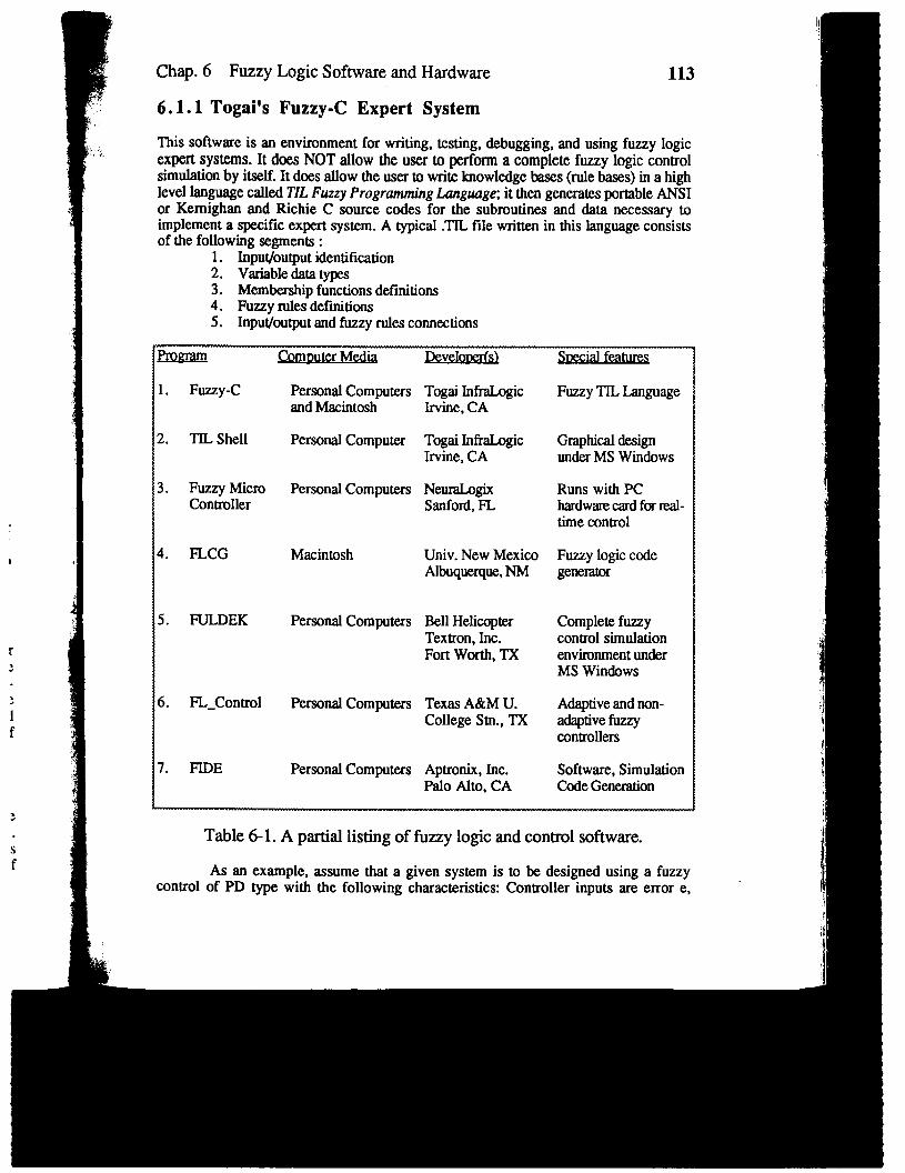
A number of fuzzy logic software programs are available in the market or at privateestablishments. These fuzzy logic software programs are summarized in Table 6-1.Perhaps the most common among these from the point of view of fuzzy control design isTogai InfraLogic’s Fuzzy-C Expert System [1]. The next section gives a briefintroduction into Fuzzy-C.
112
113Chap. 6 Fuzzy Logic Software and Hardware
6.1.1 Togai’s Fuzzy-C Expert System
This software is an environment for writing, testing, debugging, and using fuzzy logicexpert systems. It does NOT allow the user to perform a complete fuzzy logic controlsimulation by itself. It does allow the user to write knowledge bases (rule bases) in a highlevel language called TILFuzzy Programnu”ngLunguuge itthen generates portable ANSIor Kemighan and Richie C source codes for the subroutines and data necessary toimplement a ,spcific expert system. A typicaJ .TIL file written in this language consistsof the following segments:
1. Input/output identification2. Variable data types3. Membership functions definitions4. Fuzzy rules definitions5. Input/output and fuzzy rules connections
co mmner MexiM J3eveloDer@ ~ial f-
1. Fuzzy-C Personal Computers Togai InffaLogic Fuzzy TIL Languageand Macintosh Irvine, CA
2. TIL Shell Personal Computer Togai InfraLogic Graphical designIrvine, CA under MS Windows
3. Fuzzy MiCrO Personal Computem NeuraLogix Runs with PCController Sanford, FL hardwarecard fcxreal-
time control
4. FLCG Macintosh Univ. New Mexico Fuzzy logic codeAlbuquerque, NM generator
5. FULDEK Personrd Computers Bell Helicopter Complete fuzzyTextron, Inc. control simulationFort Worth, TX environment under
MS Windows
6. FL_Contzol Personal Computers Texas A&M U. Adaptive and non-College Stn., TX adaptive fuzzy
controllers
7. FIDE Personal Computers Aptronix, Inc. Software, SimulationPalo Alto, CA Code Generation
Table 6-1. A partial listing of fuzzy logic and control software.
AS an example, assume that a given system is to be designed using a fuzzycontrol of PD type with the following characteristics: Controller inputs are error e,

. .. .. ——- .. .
114 Chap,6 Fuzzy Logic Softwmead H~dwtie
change in error is DError, and the controller output is the armature voltage of a DC motoru. Assume that the error, change in error, and armature voltage have membershipfunctions shown in Figure 6-1. Moreover assume that two of the fuzzy rules are givenbelow. (1) “if e is positive mediumand DError is zero themarmaturevoltageis negativemedium,” (2) “If error is negative small and DError is positive small then armaturevoltage is zero.”
The second listing for variable error e is shown in Table 6-3. The appropriamrule base for this test example is shown in Table 64, while Table 6-5 shows the a pieceof .TIL code to conneet the input variables to the rule base and the rule base to the outputvariables.
NM NS ZE PS PM
‘“’J=JJ=”NS ZE Ps
AErrorvolts
-2 6 0 .6 2-.(b)
NM NS ZE Ps PM
ArmatureVokage
volts-lo -5 0 5 10
(c)
where NM = “negative medium”
NS = “negative srd~
ZE= “zero”Ps = “positivesmall”PM = “positivesmall”
Fi~ 6-1. Membership functions a) Input error, b) Input change in error,c) Output arrnattm voltage.
It is noted that the fde “TEST.TIL” mnsists of all the above four listings, i.e.,variable definitions, membership function, fuzzy rule M%and the conned statements. In
Chal
addifile i
prob
.
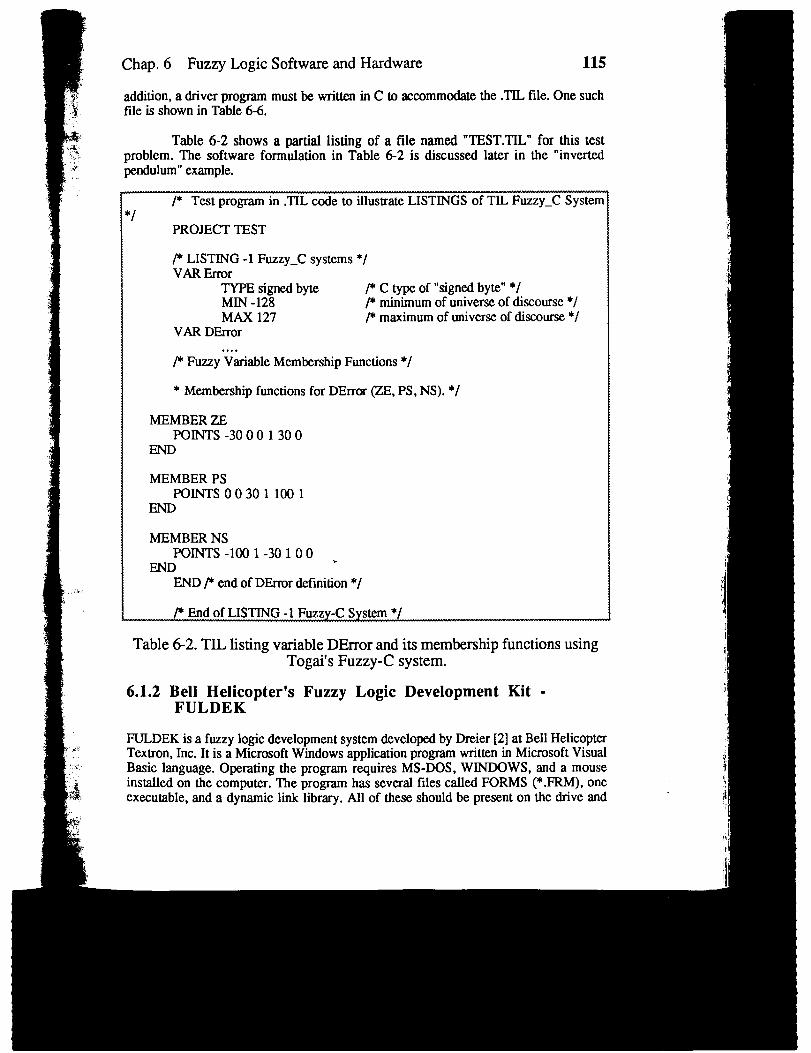
problem. The software formulation in T~ble 6-2 is discussed later in the “invertedpendulum” example.
/“ Test program in .TIL code to illustrate LISTINGS of TIL Fuzzy_C System‘1
PROJECT TEST
p LISTING -1 Fuzzy_C systems “/VAR Error
TYPE signed byte /“C type of “signed byte” “/MIN -128 /* minimum of universe of discourse*/MAX 127 /“ maximum of universe of discourse’/
VAR DError. .. .
/“ Fuzzy Variable Membership Functions*/
* Membership functions for DError (ZE, PS, NS). */
MEMBER ZEPOINTS-30001300
MEMBER PSPOINTS OO3O11OO1
MEMBER NSPOINTS -1OO1-3O1OO >
END F end of DError definition */
P End of LISTING -1 Fuzz-Em*/
Table 6-2. TIL listing variable DError and its membership functions usingTogai’s Fuzzy-C system.
‘1 )!t
..

116 Chap. 6 Fuzzy Logic Software and Hardware
directoryfrom which you plan to execute.To start the program:at the MS-DOS prompt,type: >WiN FLDK2
When all forms are loaded, the EDITOR OPTION form will appear and the useris on its way.
FULDEK has tsvo main forms, the EDITOR OPTION and the RUN OPTION.Each form has a menu bar at the top with items that can be actuated either by clickingwith the mouse or by pnxsing the ALT key in combination with the underlined letter ofthe menu item. Some menu items have drop-down menus of their own, and some of thesehave further sub-menus. The presence of sub-menus is indicated with a filled trianglebesi& the dropdown menu item.
Editor Option
To modify an existing name, “click” it in the Known Variable List. This will display thevalues of the properties in the yellow box to the right. In Figure 6-2, the variableTORQUE has been selected. The user can see at once that the TORQUE variable is an
* Test Dmrram in .TIL code to illustrate LISTINGS of TIL FUZZV-CSystem */——----.... . ..
PR6JECT TEST.-
/* LISTING -1 Fuzzy-C systems*/VAR Error
TYPE signed byte p C type of “signed byte”*/MIN -128 /* minimum of universe of discourse”/MAX 127 p maximum of universe of discourse”/
VAR DError. .. .
p Fuzzy Variable Membership Functions*/
* Membership fqnctions for DError (ZE, PS, NS). */MEMBER ZE
POINTS-30001300
MEMBER PSPOINTS OO3O11OO1
MEMBER NSPOINTS -IOO1-3O1OO
END p end of DError definition *J
c
I
(
1

—
ware
~mpt,
[ON.:kinger ofhesemgle
y theiableis an
Chap. 6 Fuzzy Logic Sottware and HaIdW~e ll”i
w Fwy IF-THEN Rules Set*/
* Rules for response */
?UZZY Alignment.rulesRULE Rule 1
IF Error IS PM AND DError IS ZE THENspeed Is NM
RULE Rule 6IF Error IS NS AND DError IS PS THENsped Is ZE
Table 6-4. TIL listing rule base for “test” problem.
*The followingthreeCONNECTObjectsspecifythat Error* and DErrorare inputs to the Alignment_rules knowledge base* and Sped output from Alignment_rules.
*I
CONNECTFROMErrorTO Alignment_rules
.
coNNEcrFROM Alignment_rulesm sped
WD
Table 6-5. CONNECT code for “test” problem on Fuzzy-C system.
. . .of 60 ft-lbs. This variable could be remov-d’ from “tie known l!isiby selecting Remove.To modify the values, the user simply “clicks” the option buttons or “clickf the numberfields and enters the value desired

II ! 118 Chap. 6 Fuzzy Logic Software and Hardware
)riVer Program c code
PFuzzy Laser Beam Tracker driver program
*I
#include “addressh”#illChl& “stdio.h”
maino
fp = fopen(datafde, “w”);
fprintf(fp, “FUZZY BEAM ALIGNMENT DATAhW’);
fprintf(fp, ‘“X-ERROR Y-ERRORh”)
for (i= Q i c= 499; ii-t)[
fprintf(fp, “%f %th; x.data[i], y_data[i]);)
fclose(fp]
printf(’ln~ile Transfer Complete.kh”); ]
rable 6-6. Drive code @lain program) to go with TEST.TIL file in Fuzzy-Csystem.
To add a variable, “clic~ New and enter the variable name. There are fourproperties which must be defined the Type property, the Evaluation property, the InitialCondition property and the Scale Factor property. Each of these is discussed below. Toselect a Type, simply “click” the desired type from the given list. Input means thisvariable is purely an antient variable. Qutput means the variable is only a conclusionvariable. ~eedb~ means the variable can be both an input and output. This meansprcxluction rules of the form:
IF XISATHENYISB
IF YISBTHENZISCcan be evaluated. Note, however, that the second rule does not receive the value of B hornthe fwst rule until the next pass through the rule base. constant means a conclusionvariable is given a constant value if the antecedent is true to any non-zero degree. Forinstance, if Y is declared a constant type and the degree of membership of X in A = mA(x)= 0.1, then rule
IF XISATHENYISBgives the function Y the fuzzy value B with membershi~ demee 1.0.

ire Chap. 6 Fuzzy Logic Software and Hardware 119
-c
)UrdTohis~onIns
]monJor(x)
Fife Name
c w
❑ei.rmg. frb ::,.,..,etgylaflb ,:::1:
fmnconl .flb.;,j:~,.:.:,:.
hw3.frb :::$,,,:.:,:hm=.frb ~openbop.hb ~<p.frbp2.frb .,.,...,...,..p3.f[b .,:,::::
P&fib.ftb ;~::
,,inl.frb w r’””‘
@c\ la
Figure 6-2. FULDEK’S Directory window.
Memberships
This sub-command lets the user edit existing membership functions or add new functions.An example of this panel is shown in Figure 6-3. All functions have four vertices at thepoints (X1,O), (X2,1), (X3,1), and (X4,0), thus only the x values are required. Thesepoints define a trapezoid, though a triangle may be created if X2=X3. There is norestriction on the X values, exmpt that the functions must be dcfmed such that Xl #X2 #x3 # x4. Thus
xl = -1.5x2= -1.0x3= -1.0 ●
x4= 4.5is a valid triangle centered at -1.0, but
xl= -1.0x2= -0.5X3= -0.8x4= -0.2
is illegal since X3 = X2.
compose
When this option is selected, the form shown in Figure 64 appears. All known “IF” and“THEN” variables are listed, as are all known membership functions. To build a rule,follow the instructions in the yellow instruction field. In general, you will follow thispath:

120 Chap. 6 Fuzzy Logic Software and krdware
IKnrmr Md.rersh@ Functions I
_NWil_ZERO_PoslD-NEG1D_ZEl10“D-POS1ORQUE..NEG2
0ROUE_POS2
Figure 6-3. FULDEKS Membership Directory window.
1.2.3.4.4a.4b.4C.5.6.7.8.
Seleqt an IF variableSelect IS or IS NOTSelect a membership functionSelect AND, OR, or THENSeleet AND, then go to Step 1Select OR, then go to Step 1Select THEN, then go to Step 5Select a THEN variableSeleet IS onlySelect a membership functionSelect END
At this point, the composed rule is displayed in the dialog box to the left.Accept itand the rule goes into the Fuzzy Rule B=, Reject it, and the rule is castaside. In either event, the user is returned to the beginning of the cycle. From here, theuser carI write another rule; search for a rule using Next, Erevious, or IJnd; Relete a
rule; or simply Return.
1.,,
/“,:
,.
,:
,:,!
,.,:
,.,:
..V
/.
,,
,
.
. .
I,.,..,,,.,....,..........,.../,.,E
~

ft.Nhe:a
H& 2 d 1 [1.]
IfTHETAisnot T_NEGl andTHETAD is TD_NEGl 01TORQUE is TORQUE_POSl
Figure 6-4. FULDEK’S Universe of Discourse Display window.
*t.:.:i.:.Methods step ~ontinuous &~DE Sim * ~eturn
.
E:...,,Figure 6-5. FULDEK’S Run Option window showing
a 3-D (control surface) plot. 121

122 Chap. 6 Fuzzy Logic Software and Hardware
Run Option
If a 3-D plot is to ke made, the Draw command will produce a surface point, an exampleof which can be seen in Flgum 6-5. The R@ate command will rotate the surface map 90degrees counter-clockwise for a different look at the surface. This command can be used asmany times as is desired.
If a God’s Eye View plot is made, then a map (Fuzzy Associate Memory, orFAM) can be obtained. Note mat unlike the 3-D graphics, the Rotate command is notactivated for this option. If an X-Y plot is made, the input variable is swept along theabscissa and the output variable is plotted as the ordinate. Again, the Rotate command isnot activated for this option. Return sends you back to the previous page, and “clicking”the Return button will return you to the RUN OPTION form.
~BCDE Sim
This sub-command allOWS you to link yow fuzzy rule base to a dynamic linear modelrepresented in state space with 5 matrices. The matrices will be discussed more in the nextchapter, but for the sake of clarity, the basic state space model reads:
dxjdt = Ax+BuYu = CUX+DUUe = Cex+Ee~
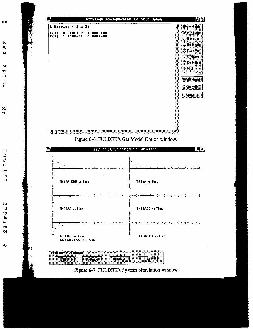
where A is the state (system) marnx, B is the control matrix, C is the output matrix andD is the feedforward matrix. Ce and Ee are the marnces to extract elemerm of the statemodel and combine them algebraically with elements of an external input vector. The “x”vector contains the dynamic states of the system and the “dx/dt” veetor is the derivative ofthe state vector with respect to time. The veetor “yu” is the output vector of the dynamicsystem and “u” is the inpfit vector. The vector “~” is the external input vector and,finally, “e” is an error v~tor. Figure 6-6 shows a Get Model Option window whichdefines the 2x2 system matrix A.
RUN ~1 M
RUN sIM aIlows the user to begin the simulation. When this option is selected, a screensimilar to that found in Figure 6-7 will appear. The abscissa and ordinates, titles, andtime will appear in the large blackboard. The user will be prompted for the time step andend time to use. Sometimes the end time will be reduced if the number of time steps istoo great, The initial conditions for the states were specified in the model date fde, so thesimulation now has all it needs to execute. When the simulation is finished, a Returnbutton will appear Wow the blackboard. “Click it to go back to the RUN OPTIONscreen.
This software will soon be available for general use. Interested readers maycontact the author directly or use the postcard at the end of the book for more details.
ue
or‘Otheis
g“
[e]:Xt
dNe
x“
oflicId,ch
enndl-dishem~N
ay
k Matrix: ( 2 x 2):* :,j~~~,tii~~lu E.::...::::”.:”
K(l) 0.000E+OO[(2) 1.61OE+O1
1.000E+OO0.000E+OO
IF
..........................................................
THETA_ERRvsTinw
[,,
I’”LT ””’
,, -,,.:: :(. ,,.
THETAD wTimeL
THETfiEIO vsTime
iiFigure 6-7. FULDEKS System Simulation window.

124 Chap. 6 Fuzzy Logic Software and Hardware
6.1.3 Fuzzy Logic Code Generator - FLCG
FLCG (Fuzzy Logic Code Generator) is an application package written for the Macintoshline of personal computers by Rashid-Alang [3] at the University of New Mexico. Itgeneratw a code in the C language (Think C by Symantee Corporation) for implementinguser-specified fuzzy logic applications. The generated code can be “attached” to a processmodel to simulate fuzzy logic control of the process. This code also writes to a defaultfilename the intermediate results of the fuzzy logic controlprogram,membershipvaluesof any input variables in the variables fuzzy subsets, the rules fued and their associatedstrengths. These results can be used to study the effectivenms or relative importance ofany rules in the controller’s ride-base.
Features of FLCG
FLCG has been written mostly for educational use and light research-oriented projects.Below are the features of this package:
. Max. number of rules :40● Max. number of variablw :7● Max. number of fuzzy subsets/vmiable :7c Fuzzification operator : Gaussian like (modif~ble) -
see Note 1● Defuzzification scheme : Simplified centroid method -
see Note 2● Fuzzy connective : AND, OR
()(X-zyNote 1. ~x) = exp - ~ .
where n is [he number of FL.Coutput variable fuzzy subsels, Ci is the centroidsof the ith fuzzy subset of the FLC output variable, Qi is the ruleactivation strength for ;he ithfizzy subset of the FLC outpu/ variable.
Structure of FLCG
The FLCG package consists of two modules: a program generator (FLCG), and a fuzzylogic function library (FLO). Figure 6-8 shows the structure of the code.

-oidsrule
He.
ware
\toshO. ItUingassfaultduesiated;e of
lzzy
I
Chap. 6 Fuzzy Logic Software and Hardware 125
THEFLCGPAC.-. —
—.— ———
GENERATEDFUZZYLOGIC CODES
—.— ——.
~~ USERSPECIFIC
I process model1 H CODES
Figure 6-8. The mchitecture for FLCG software system.
The program generator, FLCG, was compiled to form an application module. Itaccepts an input fde and generates two text files: one is a fuzzy logic program, control.c,and the other is an interface mcdule, glue.h . The interface module links the fuzzy logicprogram with the process or ptant model. The generated program and the interface moduleare plant-specflc. The input file defines the variable names, their fuzzy subsets, and thefuzzy rules used in controlling the plant. The program control.c and the plant simulationmodel can then be compiled and executed to form a complete fuzzy logic applicationprogram.
The fuzzy logic library is represented by the block FLO in Figure 6-8. Itimplements the fuzzification, rule evaluation and inferencing, and defuzzificationfunctions. This library is used by the generated fuzzy logic code. The defuzzificationscheme used is a simplified “centroid method.” In this method, the crisp control value iscalculated by taking the weighted average of the membership function with the outputvariable fuzzy subset cenhoids as the multipliers. The centroid is that point at which thearea under the membership function curve to its left equals that to its right. The five-pointGauss-L.sgendre integration method is used to calculate the area under the curve.
6.1.4 NeuraLogix Fuzzy Microcontroller NLX-230
Another software environment, from Neuralmgix Corporation [4], is called the NLX-230Fuzzy Microcontroller (NLX-230 FMC) and comes with a hardware card as well assoftware written in C language. The software package will allow you to set up your ownFAM matrix as well as the rule set. The membership functions can also be designedthrough a staircase-style biangular form, as shown in Figure 6-9.
In NLX-230 FMC the inputs are ranked by how well they fit within a set ofuser-determined membership functions. The controller uses a linear symmetricalmembership function and a simple min/max fuzzy inference scheme for easier digitalimplementation. Rules are used to determine what set of conditions is present at theinputs. Each rule consists of Up to sixteen terms, one for each crisp-input/fuzzy
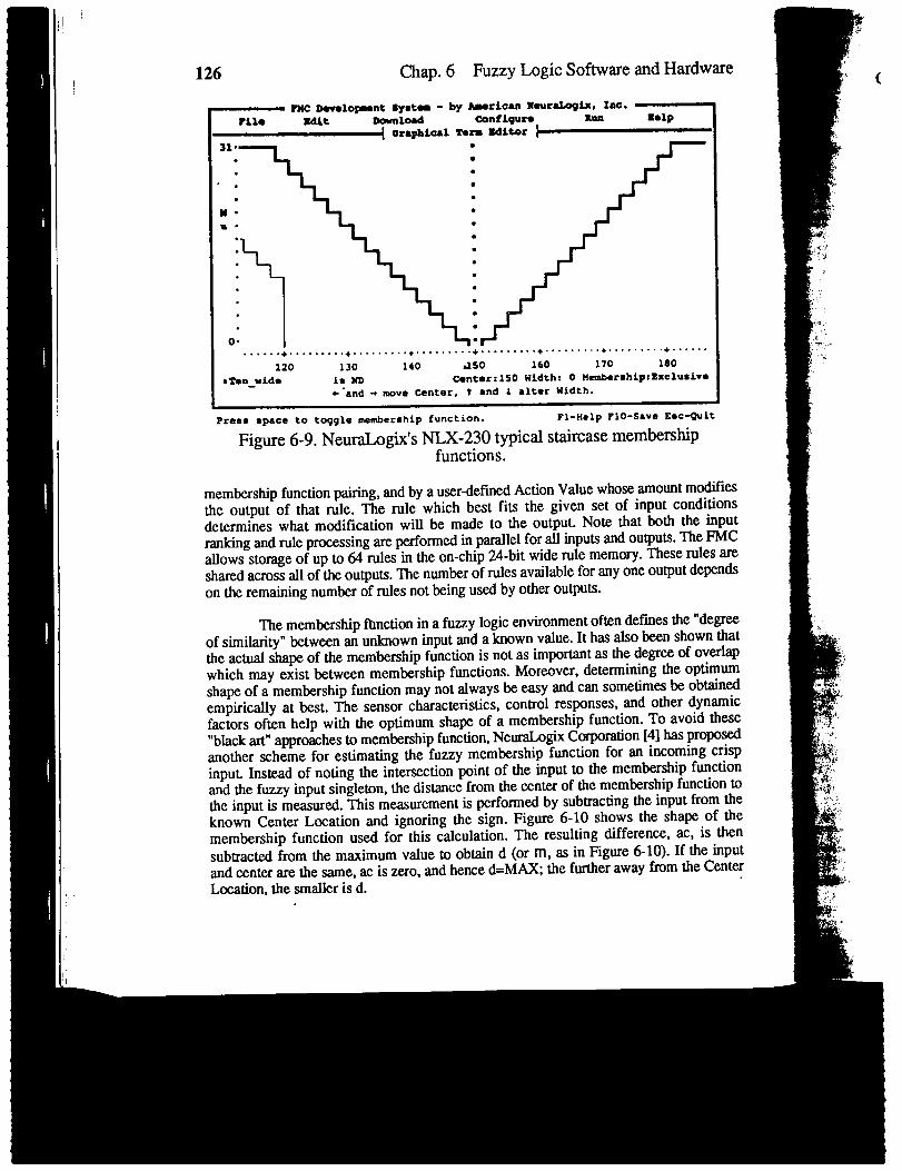
126 Chap. 6 Fuzzy Logic Software and Hardware
— Pnc Mwelopent Systa - by *rican IWurabgti, Inc. —rum adlt Download
-fiw”~~ o--”’ y ‘ii”’31.
. ●
. .
. ●
. .
M. .
m. .
.
)~~
.
. .
. .
. .
. .
. .
. .
. .
0. .. . . . . .+ . . . . . . ...+ . . . . . . . . .+....... . .+ . . - . . . ...+.... .....+..,......+. . . . . .
120 130 140 a 50 160 170 180-‘ren-wido is Ml Center: 150 Width: O Membership: Zxclusivo
+ and + move Center, t and t ●lter Width.
Prese mace to trqgle manbermhip function. F1-Help FIO-Save Emc+lt
Figure 6-9. NeuraL@x’s NLX-230 typical staircase membershipfunctions.
membership function pairing, and by a user-defined Action Value whose amount modifksthe output of that rule. The rule which best fits the given set of input conditionsdetermines what modification will be made to the output. Note that both the inputranking and rule processing are performed in parallel for all inputs and outputs. The FMCallows storage of up to 64 rules in the on-chip 24-bit wide rule memory. ‘l%eserules areshared across all of the outputs. The numb of rules available for any one output deWndson the remaining number of rules not king used by other outputs.
The membership flmction in a fuzzy logic environment often defines the “degreeof similarity” between an unknown input and a known value. It has also km shown thatthe actual shape of the membership function is not as important as the degree of overlapwhich may exist between membership functions. Moreover, determining the optimumshape of a membership function may not always be easy and can sometimes be obtainedempirically at best. The sensor characteristics, control responses, and other dynamicfactors often help with the optimum shape of a membership function. To avoid these“black art” approaches to membership function, NeuraLogix Corporation [4] hZI.SProPo~another scheme for estimating the fuzzy membership function for an incoming crispinput. Instead of noting the intersection point of the input to the membership functionand the fuzzy input singleton, the distance from the center of the membership function tothe input is measured. This measurement is performed by subtracting the input from theknown Center Location and ignoring the sign. Figure 6-10 shows the shape of themembership function used for this calculation. The resulting difference, ac, is then
subtracted from the maximum value to obtain d (or m, as in Figure 6-10). If the inputand center are the same, ac is zero, and hence d=MAX; the further away from the CenterLocation, the smaller is d.

me
t
if%ionsnputMC;are;nds
that:rlapnuminedunit
Xed:risplionm toI the‘ thethennputinter
Chap. 6 Fuzzy Logic Software and Hardware
MAX .
MIN
—— r —.= a’c
.— L —-
-A
●
Zk”mw:~c-
1 k CenterLocation
127
Xa ~ Width + X
Figure 610. Membership function shape used in NIX-230.
Figure 6-11 shows a block diagram of the circuitry used to determine similarityusing NLX-230 fuzzy microcontroller [4]. The distance value is compared against thewidth values in the Comparator. The Control Logic block is used to control data in theAlpha Cut Calculator (see Chapter 2) in the following way: if the distance is greater thanthe membemhip function, the result is forced to zero, or min. An exception to this wcu.rswhen the Typ bit is set so that it causes an exclusive membership function, so if theinput is inside, the result would be forced to min. Figure 612 shows Inclusive andExclusive membership functions with Width set at 13. If data is within the limits set byCenter Location and Width, the Alpha Cut Calculator outputs the alpha cut result.NeuraLogix claims that this method has two advantages. First, it frees the designer fromthe difficult decision of membership function determination. Second, the method produceseasily implementable solutions to the similarity determination problem.
This mehd would free the designer from choosing the shape of the membershipfunction, which is somewhat of a “black art” to begin with. It does, however, retain thedegree of overlap among membership functions which is an important aspect of fuzzylogic inferencing. It also determines a simple solution of the similarity determinationproblem [4].
6.1.5 Aptronix’s Fuzzy Inference Development Environment -FIDE
One of the more recent fuzzy logic software simulation environments is called FIDEwhich is a product of Aptronix, Inc. It is a Microsoft Windows-based environment whichwould allow the user to perform the following tasks : i) Basic functions of fuzzycomposition, inferencing, membership function composition, rule set creation and ‘

I
I128 Chap. 6 Fuzzy Logic Software and Hardware
‘np”’~
m
CenterLocation
+4’”z ‘ Calculator “
$
Control
Logic
a
-1
Type—
4
Figure 6-11. Similarity circuitry used in NLX-230.
evaluation., ii) Fuzzy control simulation , iii) Debugging of existing programs, andiv) Code generation for real-time applications.
The basic language in use for FIDE is called FIL (Fuzzy Inference Language)which is a language whi6h describes units in a fuzzy inference system. These units arecurrently FIU - Fuzzy Inference Unit, FOU - FIDE Operation Unit, and FEU - FIDEExecution Unit. FIL, as with any language such as Togai’s Fuzzy_C, has its own syntaxand semantics. For example, definition of FIU is based on the mathematical definition of afuzzy inference unit [5].
Like in FULDEK, FIDE would allow for the user to use self-generating set ofmembership functions for a given universe of discourse. This is done by a so-calledcommand listSpec as is seen in Figure 6-13. It will also allow the user to create his or herown specitlc shrqxxl membership function through the MF-Editor/Set Margin operation.
In FIDE, the system variables would appear as block within various windowswith appropriate corresponding unit such as FIU, FOU, ete. Using these block, the usercan use the Make for Simulation capability of FIDE to create a Composer/Window listwhich would be used eventually to perform fuzzy logic (control) simulation as shown inFigure 6-14. The defuzzification method used in FIDE are centroid, maximization, left-most maximization, and the right-most maximization defuzzifiers.
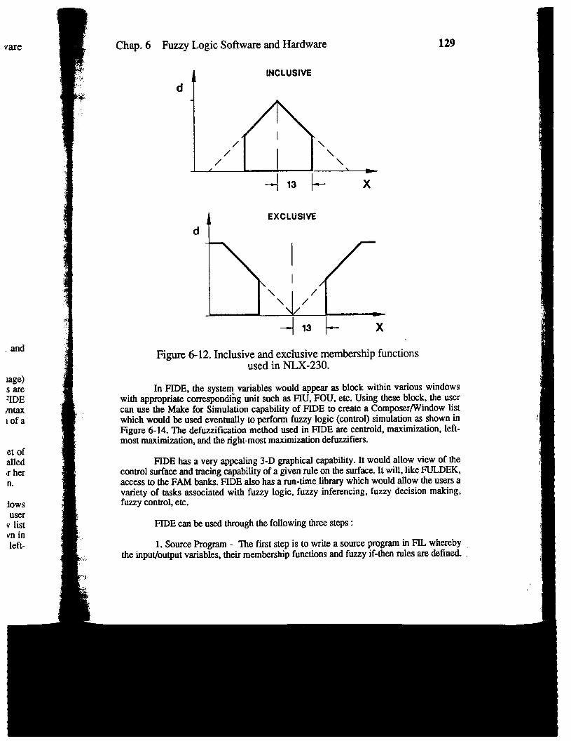
vare
, and
lage)s are~IDEmtaxIofa
et ofailed,r hern.
lowsuser
v listvn inleft-
Chap. 6 Fuzzy Logic Software and Hardware 129
d
/ \/ \
/ \1
*
EXCLUSIVE
I\
d
--ld- X
Figure 6-12. Inclusive and exclusive membership functionsused in NLX-230.
In FIDE, the system variables would appear as block within various windowswith appropriate corresponding unit such as FIU, FOU, etc. Using these block, the usercan use the Make for Simulation capability of FIDE to create a Composer/Window listwhich would be used eventually to perform fuzzy logic (conrrol) simulation as shown inFigure 6-14. The defuzzillcation method used in FIDE are centroid, maximization, left-most maximization, and the right-most maximization defuzzifiers.
FIDE has a very appealing 3-D graphical capability. It would allow view of thecontrol surface and tracing capability of a given rule on the surface. It will, like FULDEK,access to the FAM banks. FIDE also has a run-time library which would allow the users avariety of tasks associated with fuzzy logic, fuzzy inferencing, fuzzy decision making,fuzzy control, etc.
FIDE can be used through the following three steps:
1. Source Program - The ficst step is to write a source program in FIL wherebythe inputioutputvariables,their membershipfunctionsand fuzzyif-thenrules are defined.
,
I1

1!’1,~<1
130 Chap. 6 Fuzzy Logic Software artd Hardware,(1! {:1 1, In this regards, FIDE is similar to Togai’s Fuzzy_C system. Graphics interface is used!, extensively, however, to assist the user to create its FIL source code. The FIDE compiler*:
then converts the de into the APtronix standarddatastructnre.
ml 2. Code Debugging - This stage would allow the user to view the code frommultiple perspectives. Tk-w &ls are available to the user. These are: Tracer in which theuser can attach a given input variable to any test value and observe the output. This can bedone in step by step fashion similar to FULDEK. Analyzer which provides a display of aglobat view of the transfer function response. Simulator which is the final stage of theFIDEs debugger, simulates the unit’s dynamic behavior and displays the correspondingplots.
3. Real-Time Code Generation - Once a prcce.ssor has been selected, the code canbe used for a specific chip. At the present time FIDE supports the Motorola chipsMC6805, MC68HC05, and MC68HC11 and plans are for more chips to be included
At this writing, FIDE is just becoming available; hence the author has not hadthe full opportunity to evaluate FIDE completely. Interested readers may obtain the manualof this new fuzzy logic software environment [5].
6.2 SOFTWARE SIMULATED EXAMPLES
In this section we present two simulation experiences. One is the much-discussed“inverted pendulum” using Togai’s Fuzzy-C system with MATLAB [6], and the other isthe simdation of a thermal system using MATLAB’s .m file capability to create an “m”fde in place of NeuraLogix’s NLX-230 fiuzy microcontroller.
6.2.1 An Adaptive Fuzzy Control of the Inverted Pendulum
Here, a comparative study of classical expert system and an adaptive fuzzy control systemfor an inverted pendulum are given. This comparative study was done by means ofcomputer simulation through the MATLAB and Togai InfraLogic’s Fuzzy-C softwareprograms [1]. The inverted pendulum, or broom-balance problem, consists of a cart massM movable in a horizontal direction with a veloeity v, and an attached broom with massm and inertia J, whose angular displacement q and angular veloeity W could be detectedand measured. The means of balancing the broom on the cart is an external force u thatcm be applied to the cart in the horizontal direction.
The mathematical model of an inverted pendulum is well documented [7]; notethat it consists of a fourth order nonlinear unstable system. In its linearized form, it hastwo poles at the origin, one in the right-hand plane and one in the left-hand plane. Thesystem was linearized about the region –5° <= q <= 5° and then a state feedbackcontroller was designed for it. This pole placement was done by a full state feedback suchthat u=Kx, and K’s were determined such that poles were placed at -2,-1, and -l*j. By
1 virtue of the definitions of the svstem’s states. this state feedback controUer is effectivelya PD controller. The plant was made stable with this controller.
r(,,
.,I
w;
1
(
.,,,,
,.
.,!.\.:..
*
..
. .
h
,,

re
dler
lmhebe
h:ag
anps
add
ds,,
nIfess‘dlt
esekhYY
Chap. 6 Fuzzy Logic Software and Hardware 131
Adaptive Fuzzy Expert Control System
In an attempt to improve the response of the system, a variable feedback (self-tuning)controlled was designed. In order to acquire the knowledge base the state feedback gainswere changed during the simulation. It was experimentally discovered that in order toobtain the greatest impact on the stability and response of the system it was necessary tovary only K2 and K3 state feedback coefficients, which actually corresponds to the changeof the cart velocity and the angle of the broom. In order to see “real” improvement of thesystem, the angle q was limited to change *9, and the change of the displacement of thecart tot 0.5 meters, so that the problem could k potentially implemented in hardware ona l-meter track. The ida behind the expert system design is that if a large displacementwas detected in the output of the plant, a big state feedback value would be applied tocontrol the pkm~ and vice versa. If small q displacement is detected, small state feedbackwould be applied. With this methcd, the overshoot of the system would be improved,while the time response of the system would be increased.
Both the constant controller and the expert system controller are “crisp” systems,i.e., both have certain crisp values for the state feedback controller in response to certainangular displacement. With the fuzzy system it is possible to have an adaptive controllerfor the dynamic system, but this controller will change for all the intermediate values ofangular displacement that were not implemented before; moreaver, this change will benonlinear in response to the nonlinear dynamic system.
Frost, the input and output fuzzy variables were determined. Previously, it wasdetermined that the best con@ol for the system is achieved by adjusting X2(cart velocity),and X3 (angular displacement) states. Therefore, these two states will be our sensor
outputs from the fuzzy controller. These outputs are designatedas K2FACand K3FAC,respectively.From previous experimentingwith the expert system, limitations on thesevariables were determined as: q for t ~; K2FAC and K3FAC 1-2 (this is just themultiplication factor). The purpose of the fuzzy controller is to improve the settling timeand the stability of the system.’Another advantage of this system is that a previouslyacquired data knowledge base can be used, except now the mapping for the state feedbackelements will be nonlinear.
Nex~ the membership functions for each variable must be assumed using typicaltrapezoidal at the ends and a triangular in between the intervals. The membershipfunction for q is evenly spread between +5o and –50 degrees over seven regiow. negativebig, medium, and small; zerq and positive big, medium, and small. K2FAC and K3FACmembership functions are equal, but unevenly spread over four regions: positive small,medium, big, and wide. ‘l%e reason for the uneven spread is that we need a lot ofcompensation when q is *3 degrees or bigger, but as q gets smaller, less compensationand more “finesse” are needed in the compensation because we want the system to settlequickly and with the minimum overshoot. Therefore the membership function is denserand more overlapped for small Ks so we can achieve a “linear” effec~

132 Chap.6 Fuzzy Logic Soflwa.re and Hwdwa.re
NexG determine fuzzy rules for the system. This is done by mapping q member-ship function into K2FAC and K3FAC membership functions. Therefore, mapping isdone as follows:
1. when THETA is PB or NB, Ks am mapped as PW (very big compensation)2. when THETA is PM or NM, Ks are mapped as PB (big compensation)3. when THETA is PS or NS, K’s are mappal as PM (medium comp.)4. when THETA is ZO (close to zero), K’s are mapped as PS (small
compensation).
Simulation and Results
The simulation of the expert and fuzzy expert control systems were done by interfacingMATLAB and Togai InfraLogic’s Fuzzy-C expert system environment. Figure 6-13shows the simulation approach. The Togai’s fuzzy controller was used in conjunctionwith MATLAB’s differential equation solvers (ode45.m) capabilities to complete the fkzycontrol systems simulation. The former environment is used to simulate the dynamicbehavior of the system, while the latter represents an environment for the fuzzy controller(rules, membership function conflict resolution, etc.). The connection between the twosimulation environments was made through the C-language shell which allowedMATLAB and Fuzzy-C to communicate. ‘Ile system’s simulation was done in threestagex 1) Constant feedback control system, 2) Expert control system, and 3) Adaptivefuzzy expert control system.
MATLAB
Pend.EXE
1
FCC
Fuzzy C Compiler C-Compiler
Togal Fuzzy-C Expert Syetem
Figure 6-13. A combined Fuzzy-C expert system andMATLAB simulation.
A typical simulation result is shown in Figure 6-14. The time response forangular position is shown here for all three controllers. It is noted that under the exWrtsystem controller, both overshoots and settling times consistently worsened for theangular displacement.The thid simulation was done when fuzzy IF-THEN rules and themembership functions were used to tune the controller’s gains. Both the overshoots andsettling times improved. Also shown in Figure 6-14 are the usual smoothing andinterpolation effects of fuzzy rules in between crisp expert rules. It is further noted thatboth the overshoot and settling time have been improved through the fuzzy expertcontroller. The comparison between these two controllers is also in favor of the fuzzy
Cha~
contrlincre.simulplace
3,
~
1 ~
o
-1
_~ \
-3
-..4
.-~(
6.2
In 1Neuapprelaprolopel
Y(5conchathe
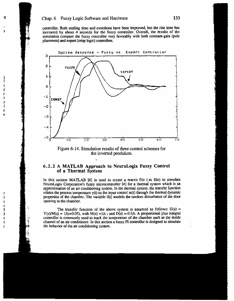
Chap. 6 Fuzzy Logic Software and Hardware 133
controller. Both settling time and overshoot have km improved,but the rise time hasincreased by about 4 seconds for the fuzzy controller. Overall, the results of thesimulation compare the fuzzy controller very favorably with both constant-gain (poleplacement)andexpert(crisplogic)contmlkrs.
System Response - Fuzzy vs. ~xpert Controller
3.
~J
1
0 -
-iCflNST
-2
3 -
-4
-,~ 1~o 1.() ;! o :)() 4() !i () (1 o
Figure 6-14. Simulation results of three control schemes forthe inverted pendulum.
>
6.2.2 A MATLAB Approach to NeuraLogix Fuzzy Controlof a Thermal System
In this section MATLAB [6] is used to create a macro file (.m file) to simulateNeuraLogix Corporation’s fuzzy microconmoller [4] for a thermal system which is anapproximation of an air conditioning system. In the thermal system, the transferfunctionrelates the process temperaturey(t) to the input controlm(t) throughthe thermaldynamicproperties of the chamber. The vtible d(t) models the random disturbance of the dooropening to the chamber.
The transfer function of the above system is assumed as follows: G(s) =Y(s)/M(s) = 1/(s+0.05), with M(s) =1/s ; and D(s) =-0.5/s. A proportional plus integralcontroller is commonly used to track the temperature of the chamber such as the insidechannel of an air-conditioner. In this section a fuzzy PI controller is designed to simulatethe behavior of the air conditioning system.
134 Chap. 6 Fuzzy Logic Software and Hardwwe
First, to acquirea knowledgebase regardingthe plant characteristics,the systemwas run througha seriesof simulationsusinga varietyof disturbances 1)no disturbance,2) a continuousdisturbanceof 1, 3) a delayeddisturbance,and 4) a puked disturbance,.Due to lack of space most of the simulation results are not presented here. More detailsan be obtained from Reference [8],
The system simulation results showed the system to be stable, exhibiting aclassical overdamped step response. The injection of the disturbance input in each casesignificantly affects the system’s ability to achieve a target tem~mture. The disturbanceinput alters system temperature trajectory with overdamped characteristics. Since thesystem bandwidth is small, closing the loop with a P (proportional) controller willeffectively increase the bandwidth, improving transient response. However, the PI(proportional-integral) controller is itself a low pass filter which forces the steady state
error to zero; this improves disturbance rejection but may in fact degrade the transientresponse in the process. Hence, the design question “How do we adaptively change the PIcontrol gains to optimize overall performance?” The answer lies in the knowledge basethat interprets the PI controller’s frequency response.
API controller has the following transfer function: Gc(s) = Kp + Ki/s = (KP.s +Ki)/s, depending on the Ki/KP ratio, the system dynamics-overshoot, rise time, andsettling time change. The PI controller adds low frequency gain to increase the systembandwidth, forcing the steady state error to zero, as well as adding a low frequency phaseto destabilize the system. Adjusting the gain ratio also affects the position of the closedloop poles, which directly affects the overshcd, rise time, and stability of the system.
The characteristic equation set the pole locations as follows: p(s)= S2+ (0.05+ Kp). s +Ki. Note the followingobservations:
1) If K~Ki poles remain on the real axis, there is no overshoo~2) ASKP<Ki poles leavereal axis and overshootwillUCCUGand3) As Kp is set larger than Ki the dominant pole approaches the Origin leading
to a slower transient response.
With this ffequen;y and root locus information to form a preliminary knowledge,the next task is to address the simulation model governing the system, with attention tothe details of control resolution, and finite computation precision. Figure 6-15 shows ablock diagram of an adaptive fuzzy PI control for the thermal system. The system has thefollowing numerical description: Sensor was assumed to be represented by 0.05 v/Co,DAC by 4096 bits per 5 volts, ADC by 24 volts per 4096 bits, and set point by 40degrcss c.
In facing the issue of con@ol, fuzzy or non-fuzzy ,the degree to which theoutputs can be measured sets the limitations on how well the system will eventually becontrolled. Since most conmol and all adaptive/algorithm-based control is done digitallythere is a need to quantize the effects of digitization.
In choosing the rule setimembership functions for the adaptive PI controller, theprevious information regarding the pole locations and tlequency response was considered.Figure 6-16 shows the membership functions of the absolute error for time peried n andn-1 to be used for the subsequent simulation.
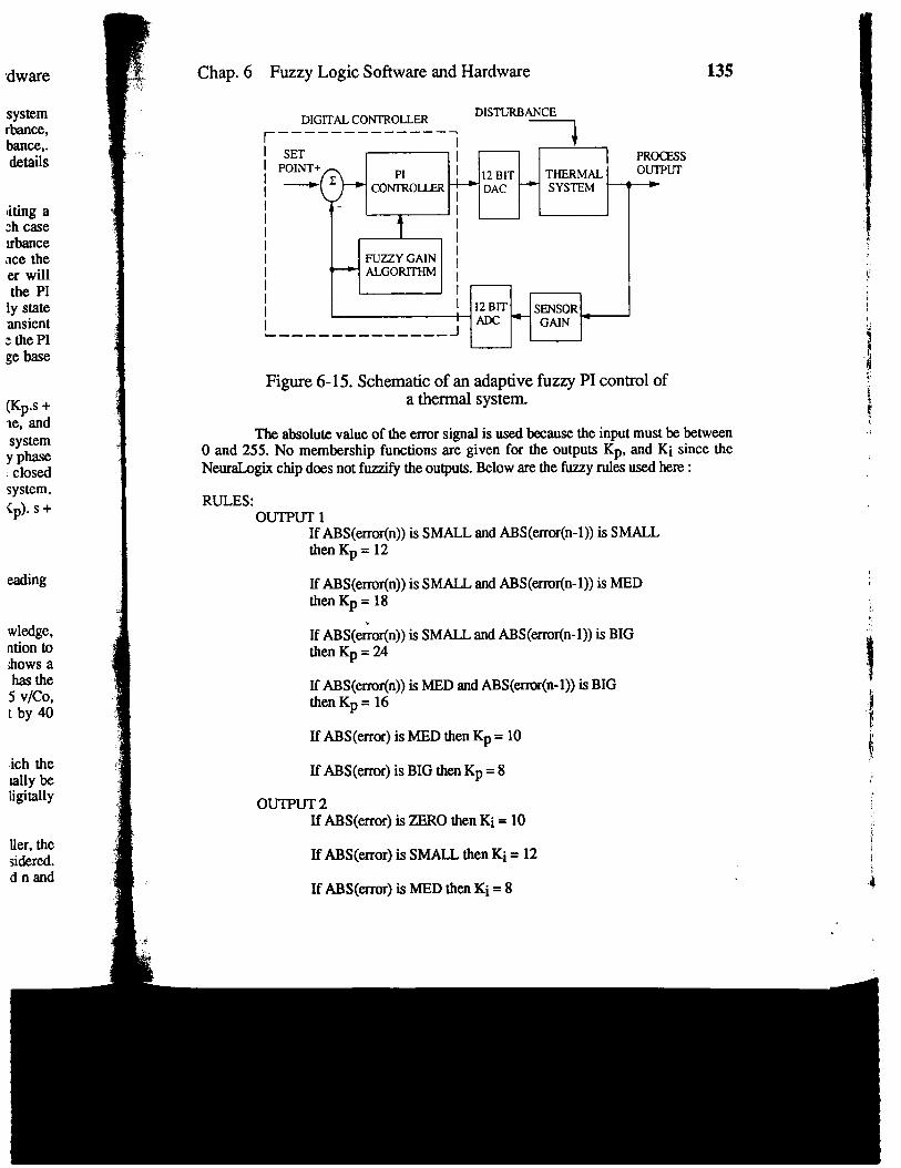
“dware
systemrbanee,
details
Bitinga:h casembanceace theer willthe PI
ly stateansientz the PIge base
(Kp.s +oe, andsystemy phase. closedsystem.Cp). s +
eading
wledge,ntion toJIows ahas the5 Vlco,t by 40
ich thelally kIigitally
her, thesi&red.dnand
Chap. 6 Fuzzy Logic Software artd Hardware
DIGITAL CONTROLLERDISTURBANCE
~_––– ————.———— .
I SETI 1
~1 ~ I
I
IIiI
IIIk———
EFUZZY GAIN ,ALGORITHM ,
II
———- —————— J
PROCESSOu-rtlrr~
=E=l-
135
u—
Figure 6-15. Schematic of an adaptive fuzzy PI control ofa thermal system.
The absolute value of the error signal is used because the input must b betweenO and 255. No mem~rship functions are given for the outputs KP, and Ki since theNeuraLogix chip does not fu.zzifythe outputs. Below are the fuzzy rules used here:
RULES:OUTPUT 1
If ABS(emr(n)) is SMALL and ABS(error(n-1))is SMALLthen Kp= 12
If ABS(error(n)) is SMALL and ABS(error(n-1))is MEDthen Kp= 18
If ABS(e&x(n)) is SMALL and ABS(error(n-1))is BIGthen Kp = 24
If ABS(ermr(n)) is MED and ABS(error(n-1))is BIGthen Kp = 16
If ABS(error) is MED then KP = 10
If ABS(error)is BIG then KP = 8
OUTPUT 2If ABS(error) is ZERO then Ki = 10
If ABS(emor) is SW then Ki = 12
If ABS(error)is MED then Ki = 8

;,,>\’,,. ‘.
II1.,;I1.,
136 Chap. 6 Fuzzy Logic Software and Hardware
The foUowing observations should now be noted:
~’~90
ABSOLUTE VALUE OF ERROR(n)
I I SMALL MED BIG
I 1 II
i’10 30 50
ABSOLUTE VALUE OF ERROR(n-1 )
Figure 6-16. Membership functions for the absolute errors for the
Ithermal system.
IThe following simulation made use of the error signal at time (n) and the error
signal at time (n-1), in order to provide more information to the fuzzy rule base and thusimprove results. The simulation was ~rformed using the membership function fromFigure 6-16 and the fuzzy rules just presented. Figure 6-17 shows the new step responses
1 of the thermal system using both fuzzy and crisp PI controllers.
I The simulation shows that the fuzzy controller does reject disturbances moresmoothly, but the crisp PI is fairly adequate as well.
I
;:3.
4.
5.
6.7.
The error signal is the only input that determines outpuLs.All outputs are integers,The output values for Kp and Ki change in unison since they U~ tie same
input.The changes in Kp and Ki are always such tit K@Ki, kwping the POleSonthe red axis.When the error signal is large K@i values are large to increase the controlsignal to the plant.As the error signal rcxhws., K&i values reduce to prevent overshcmt.When the error signal is small Kp/Ki are large for increased sensitivity
I SMALL MED BIG
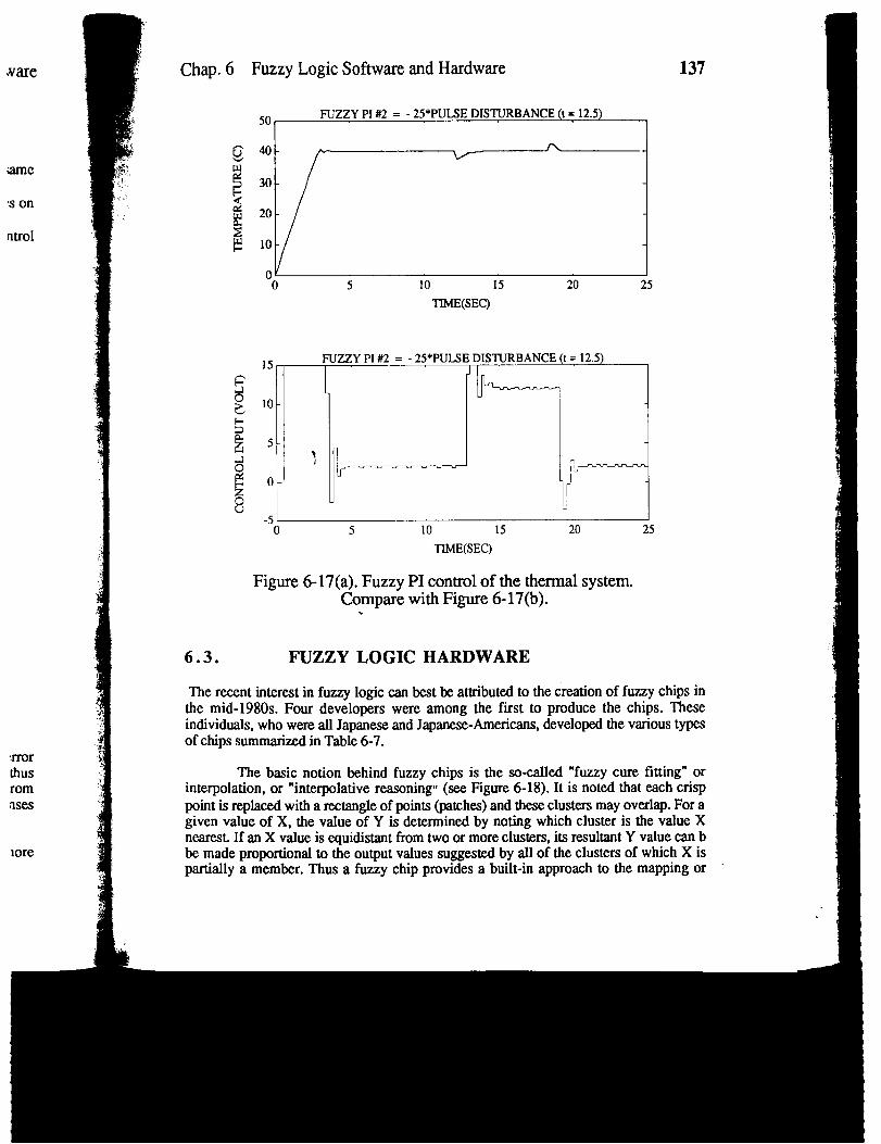
rrorthusromfises
lore
Chap. 6 Fuzzy Logic Software and Hardware
50 FUZZYPI #2 = - 25* PULSE DISTURBANCE (t= 12.5)
g’$o - h
!
w
30 -
~ 20 -
2
137
1oo~25
TIME(SEC)
15 FUZZY PI #2 = - 25* PULSE DISTURBANCE (t= 12.5)
10-
5 -)f
o J
\-
7IL
/
-5Io 5 10 15 20 25
TtME(SEC)
Figure 6-17(a).Fuzzy PI control of the thermal system.Compare with Figure 6-17(b).
.
6.3. FUZZY LOGIC HARDWARE
The recent interest in fuzzy logic can best be attributed to the creation of fuzzy chips inthe mid- 1980s. Four developers were among the fwst to produce the chips. Theseindividuals, who were all Japanese and Japanese-Americans, developed the various typesof chips sumrnariti in Table 6-7.
The basic notion behind fuzzy chips is the so-called “fuzzy cure fitting” orinterpolation, or “interpolative reasoning” (see Figure 6-18). It is noted that each crisppoint is replaced with a rectangle of points (patches) and these clusters may overlap. For agiven value of X, the value of Y is determined by noting which cluster is the value Xnearem If an X value is equidistant from two or more clusters, its resultant Y value can bbe made proportional to the output values suggested by all of the clusters of which X ispartially a member. Thus a fuzzy chip provides a built-in approach to the mapping or “
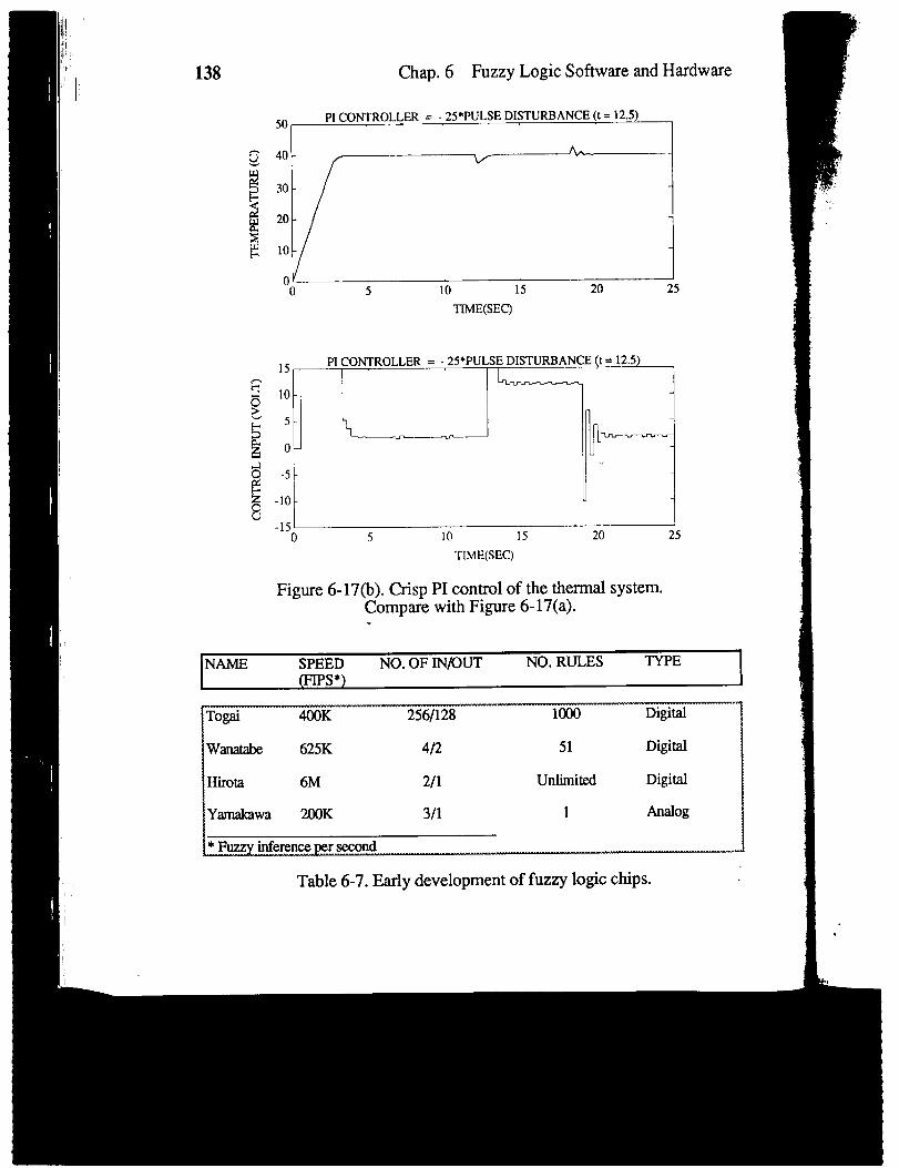
138 Chap. 6 Fuzzy Logic Software and Hardware
50 PI CONTROLLER = - 25* PULSE DISTURBANCE (t= 12.5)
40 - vA.
30 -
20 -
10 - 1
o~o 5 10 15 20 25
TIME(SEC)
15PI CONTROLLER = - 25*PULSE DISTURBANCE (t= 12.5)
I
-5 I
-lo I
I 1
H1‘“
-15~o 5 10 15 20 25
TJME(SEC)
Figure 6-17(b).Crisp PI control of the thermal system.Compare with Figure 6-17(a)..
INAME SPEED NO. OF IN/OUT NO. RULES TYPE II @’pcJ*) I
Ya.malmwa 200K
Table 6-7. Early development of fuzzy logic chips.

[ware
[J
k
Chap. 6 Fuzzy Logic Software and Hardware 139
interpolationproblem. It is noted that in more recent time, many other fuzzy chips eitherhave come or soon will be coming into the market. Notable among these are OmronCorporation and NeuraLogix as well as Motorola, Inc. Space and time are not availablehere to give a &tailed discussion of these chips, however two fuzzy cards which have beenused at University of New Mexico’s projects will be discussed below: the Togai Single-Board Fuzzy Conhdler and the NeuraLogix Fuzzy Microcontroller.
INTERPOLATIVE REASONING
(lFXisA~YlsB]
Y
a
/’-filzzy output
/
AL fuzzy input
Figure 618. The notion behind fuzzy chips: Interpolative Reasoning.
6.3.1 Togai Single-Board Fuzzy Controller
The single-board fuzzy controller (SBFC) comes with the standard Togai fuzzy chip (seeTable 6-7) and its own A/D and D/A chips, as well as the 230 standard BUS and otherinterface. It has a 1-Mbyte erasable and elechicall y programmable ROM (EPROM).Software is available which translates the fuzzy expert control system developed by TogaiFuzzy-C into machine code for the miaoprocessor used on the board. Over 800 rules canbe supported in the hardware and up to 200,000 fuzzy rules can be evaluated in onesecond. The programming procedure for the SBFC is similar to that of programming inFuzzy-C on a PC. There are, however, some very distinct differences. Programming inFuzzy-C on a PC, the standard Fuzzy-c de can be used as a debugging tool and a checkon the hardware implementation. In using SBFC the fuzzy programming tanguage (FPL)code is compiled directly to an object code. The driver code (main program) is written inFC110 assembly code instead of C, as in the Fuzzy-C system. The FC110 assembler isused to convert the driver to an object code, and the FC 110 linker can then be used tocombine the two object codes into a code that is executable by the FC 110 digital fuzzy .processor (DFP). This procedure is described in Figure 6-19.

140 Chap. 6 Fuzzy Logic Software and Hardware
v “+FCI 10 FPLCompiler
—
FCIIOAssembler
FCIIO LINKER II !
EE!!E3Figure 6-19. Steps for creating hardware ready fuzzy control program.
It is possible to interfaee the SBFC board with a personal computer.For verycomplkated contiol programs this may be the best way to develop and debug the codes.Results of a reeent project by Shao and Parkinson [9] showed that it is not necessary tobuild an interface if the user-developed assembly de is used only for interacting betweenthe hardware components on the board and the fuzzy rule codes. Since fuzzy rule bases canbe easily deveIoped with the aid of the Fuzzy-C development systems software mentionedearlier, a complicated red-time fuzzy control system can still be implemented using thecode described here. The followirm steps summarize the programming of Togai’sSBFC:
1.2.3.
4.5.
6.
Set public and extem-al s~mbols - -Initialize the stackpointer used for calling subroutinesLoad sensor input from A/D converter address to the fuzzy rule routine inputvariable address.Call the fuzzy rule routineLoad conrrol output from the fuzzy rule routine output variable address tothe D/A converter address.Go to step 3.
Ch
:
rok
6.
Inin~blo~:inpfuzproper23(
ofassFig
higof 1rekOu[

Iware
m.
mverycodes.‘~ to:tweenK-scanItionedmg theMC
: input
ress u)
Chap. 6 Fuzzy Logic Software and Hardware 141
INTERFACELOOP BACK # I
I
fiwiw=Figure 6-20. Block diagram for NLX-230 fuzzy microcontroller.
In a later section Togai’s SBFC is used to control a conveyor belt system inrobotic assembly application. -
6.3.2 NeuraLogix Fuzzy Microcontroller
In an earlier section the NeuraLogix NLX-230 fuzzy microcontroller was brieflyintroduced. Here a few more words will be given regarding the card itself. Figure 6-20, a
block diagram of the NLX-230 FMC, shows that there are 16 fuzzifiersassociatedwiththis controller.Eachof these fuzzifiershasa l-of-8 selectorwhichallowseach fuzzifiertoinput data from any one of the eight inputs. Each fuzzifier looks at only one input. If afuzzifier is configured to be used in a Loop Back from an outpug then it cannot be used toprocess an external input. This conjunction of an input with a membership functionperformed by a Fuzzifier is called a “Term” by Neural.ogix Corporation [4]. The NLX-230 supports a maximum of 16 such “Terms.”
Each fuzzifier, using the similarity notion discussed earlier, calculates the valueof the membership function for its input signal. There is an 8-bit Center Locationassociated with each Fuzzifier. Membership values which fall within the Width (seeFigure 6-10) are passed onto the Minimum Comparator for rule processing.
The Minimum Comparator block is implemented with a Neural Network forhigh-sped throughput. The fwst 16 bits of the 24-bit rule are used to enable the outputsof each fuzzifier to compare the minimum merrdxrship values. Each rule bit has a fixedrelationship with a fuzzifler. When a rule bit is asserted “1,“ the corresponding Fuzzifieroutputs are compared with one another to find the minimum value.
&
i
142 Chap. 6 Fuzzy Logic Software and Hardware
Once the minimum value for a rule is found, it is stored in a temporarymaximum register in the Maximum Comparator. The minimum value of each rule beingprocessed is compared against a reference value stored in the maximum register. Afterprocessing all of the rules, the resulting value in the maximum register is the maximumvalue of all the minimums. This value represents a “fuzzy” logical sum-of-products. Thewinning rule’s Action Value is passed on to the defuztification control. The Action Valueis an 8-bit two’s complement value ranging from -128 to 127.
The 8-bit Action Value from the rule memory word is added to a user-definedInitial Value. For example, an Initial Value of 100 added to an Action Value of –5 wouldresult in an output value of 95. Saturable arithmetic is used to keep the input value from“rolling over” (modula 128) in the event adding an Action Value attempts to increment ordecrement the Output Value past the upper or lower boundary (-128 and 127). The OutputRegisters are pipeline.dto enhance performance. Once all the rules have been processed andthe outputs have been defuzzified, the device begins clocking out the data whilesimultaneously entering the next group of data inputs. In this way the NLX-230 does notuse the traditional centroid method for fuzzification.
This card has been used at UNM’s CAD Laboratory for three applications of real-time control of systems, including the conveyor belt discussed in the next section, butresults were not available in time for inclusion here. Future publications will incorporateNLX-230S real-time implementations.
6.4 HARDWARE EXPERIMENT EXAMPLES
This section will briefly discuss two real-time fuzzy controller implementations designedin a laboratory setting. Currently, four real-time control architectures are beingimplemented for real-time fuzzy control systems. Figure 6-21 gives a pictorialpresentation of all four implementations. As shown, three are based on Togti InfraLogic[1] software and hardware and the fourth is based on NeuraLogix’s FMC board [4].
6.4.1 A Conveyor-Belt Experiment - Fuzzy-C Approach
Figure 6-21(a) shows the experimental set-up for the control and tracking of a roboticstation’s conveyor belt using self-tuning fuzzy PI controller. The fuzzy controller wasimplemented on a Packard Bell 386 personal computer, which acted as host for theTogai’s Fuzzy- C expert system. A user-interactive program was written to prompt theuser with data for the fuzzy ecmtroller implementation, Fuzzy IF-THEN rules were used toautomatically adapt the gains of the PI controller in rcaetion to system disturbances andunmodelled dynamics. For example, one experiment dealt with various load conditionsand sudden load changes on the conveyor belt, The conventional controller acted relativelysatisfactorily for low load, but the fuzzy controller could adjust promptly for any loadsituation, including high load. Typical rules were:
fF ERROR IS NB OR PB THEN GAIN IS PBELSEIF ERROR IS NS OR PS THEN GAIN IS PSELSEIF ERROR IS ZERO THEN GAIN IS PM
c
.s:buba
6
h-rttwt]i]
Fdi:ilsilC(irt\
6
sLh:0101
air~C(b!2

Iware
KNary
beingAfterimums. TheValue
finedwould: fromlent or)utputxl andwhilees not
‘freal-n, butporate
;ignedbeing:torial,Logic
Obotic:r wasor thept thelsed tos andlitionstivelyy load
Chap. 6 Fuzzy Logic Software and Hardware 143
The correspmding membershipfunctionsfor GAINand ERRORwerechosen asstandard trapezoidal at the two ends of the interval and an overlapping triangular inhxween intends. Figure 6-22 shows the error behavior for load and no-loadconditionsusingPI (crisp)and fuzzyPI controllers,Although this system was fairly linear and well-twhavtxi, and the true nature and power of fuzzy logic cannot be tested, it did allow theauthors to realize a real-time control implementation .
6.4.2 A Conveyor-Belt Experiment - SBFC Approach
In this section the czmveyor belt system of the previous section is controlled using theTogai’s SBFC car~ which was also described earlier. The goal of the experiment remainedthat of controlling the speed of a DC motor driving a conveyor belt. The speed of the beltwill vary under load and no-load conditions. The sensed input is the speed of the motor inthe form of a voltage from a tacho-generator. The rules base for the hardwareimplementation are given by the following set of four rules [9]:
1. IF the input voltage is VLC)W (very low) THEN output voltage is HIGH2. IF the input voltage is LOW THEN output voltage is MEDIUM3. IF the input voltage is MEDIUM THEN output voltage is LOW4. IF the input voltage is HIGH THEN output voltage is VLOW
The input and output voltage membership functions are shown in Figure 6-23.For verifkation purposes me input/output rules for the fuzzy controller were simulated onthe Fuzzy-C system. The resulting input/output of the fuzzy controller using simulationis shown in Figure 6-24. Then the SBFC implementation of the conveyor bel~ as shownin Figure 6-25, was performed using the steps outlined in the section headed “TogaiSingle-Board Fuzzy Controller.” The resulting hardware implementation of theinput/output of the fuzzy controller is shown in Figure 6-26. Note the closecorrespondence between this figure and the curve in Figure 6-24. Disregard the discrepancyin the scaling of the axes of the latir figure; this was done for ease of plotting, and thetwo scales are in fact the same.
6.5 CONCLUSIONS
Since 1989 many software and hardware projects have been undertaken within the CADLaboratory at the University of New Mexico, where all of this books txlitors and authorshave worked. The projects discussed here represent signiilcant progress in the applicationsof fuzzy logic to control, pattern recognition, digital faltering, and other areas. The detailsof these projects appear in Chapters 7 through 18.
One important projec~ which at this moment is not quite ready for reporting, isa fuzzy PI Control of a non-CFC based air-conditioning system. This project, developdin collaboration with 10cal industry, attempts to implement an adaptive fuzzy PIcontroller for a newly patented non-freon based air conditioning system for trucks andbuses. The controller will be based on the NeuraLogix fuzzy microcontroller ~lgure 6-21[d]).

144 Chap. 6 Fuzzy Logic Software and Hardware
We conclude by once again noting that it is difficult for a single chapter to coverthe wide spectrum of software and hardware currently available in the marketplace Wehope the reader will take this chapter as an initial reference for further reading and re-searehinto this important aspect of fuzzy logic and fuzzy cxmtrol.
ACKNOWLEDGMENTS
The writing of this chapter would not have been possible without the remarkable work ofso many of the author’s capabIe students. Thanks to Mr. Denis Barak, Mr. Narul Rashid-Alang, Mr. Steve Baugh, Mr. Jinqiu Shao, and Dr. Jerry Parkinson for their manydedicated hours of work. The collaboration of Mr. Mark Dreier of Bell Helicopter Textronis also sincerely appreciated. Ftiy, deepest gratitude goes to Dr. Lotil Zadeh, the fatherof fuzzy logic, for his generous encouragement.
REFERENCES
[1]
[2]
[3]
[4]
[3
[0
[7
[8]
[9]
Togai InfraLogic, Inc. Fuzzy-C Expert Systems User’s Guide, 1990, Irvine, CA,1990.
M. Dreier. FVLDEK - Fuzzy Logic Development Kit User’s Manual, Bell HelicopterTextron, Fort Worth, TX, 1992.
N. Rashid-Alang. FLCG - A Fuzzy Logic Co& Generator, Technical ReportDepartment of Chemical and Nuclmr Engineering, University of New Mexico,Albuquerque, NM, 1992.
NeuraLogix Corporation. User’s Guidefor NLX-230 Fuzzy Microcontroller. Sanford,FL, 1991.
Aptronix Corpomtion. User’s Guidefor FJ.DE Fuzzy Inference DevelopmentEnvironment, Palo Alto CA , 1992..’
Mathworks, Inc. MATLAB User’s Guide. Boston, MA, 1991.
M. Jamshidi, M. Tarokh, and B. Shafai. Computer-Ai&d Anaiysis and Design ofLinear Control Systems. Prentiee Hall Publishing Company, Englewood Cliffs, NJ,1992.
M. Jamshidi, R. Marchbanks, K. Bisset, R. Kelsey, S. Baugh, and D. Barak.“Computer-Aided Design of Fuzzy Control Systems,” in Advances in Computer-AidedControl Systems Engineering, M. Jarnshidi and C. J. Herget (Eds.). North- HollandPublishing Company, Amsterdam, 1993.
J. Shao and G. Parkinson. “programming and Testing of the Togai Single-BoardFuzzy Controller,” Internal Refirt, C~- Laborato~-for Intelligent and RoboticSystims, University of New Mexico, Albuquerque, NM, 1992.

4-nctuatooutput
i,
copter
nford,
m“>/A TOGAIFUZZY.c tlctuotor
SYSTEM output I
I
(a)
m ““or+&1CONTROL
sensor
SOFTWARE input
AID
(c)’
sensor
(b)
Neura LoglxNLX-230 FUZZYMicrocontroller
input
I
sensor
Figure 6-21. Four real-time archkctures for fuzzy control systems:(a) Software Implementation (Fuzzy-C); (b) Togai SBFC;
(c) Toga.iFS110 System, and (d) Neuralmgix’s NLX-230 FMC.
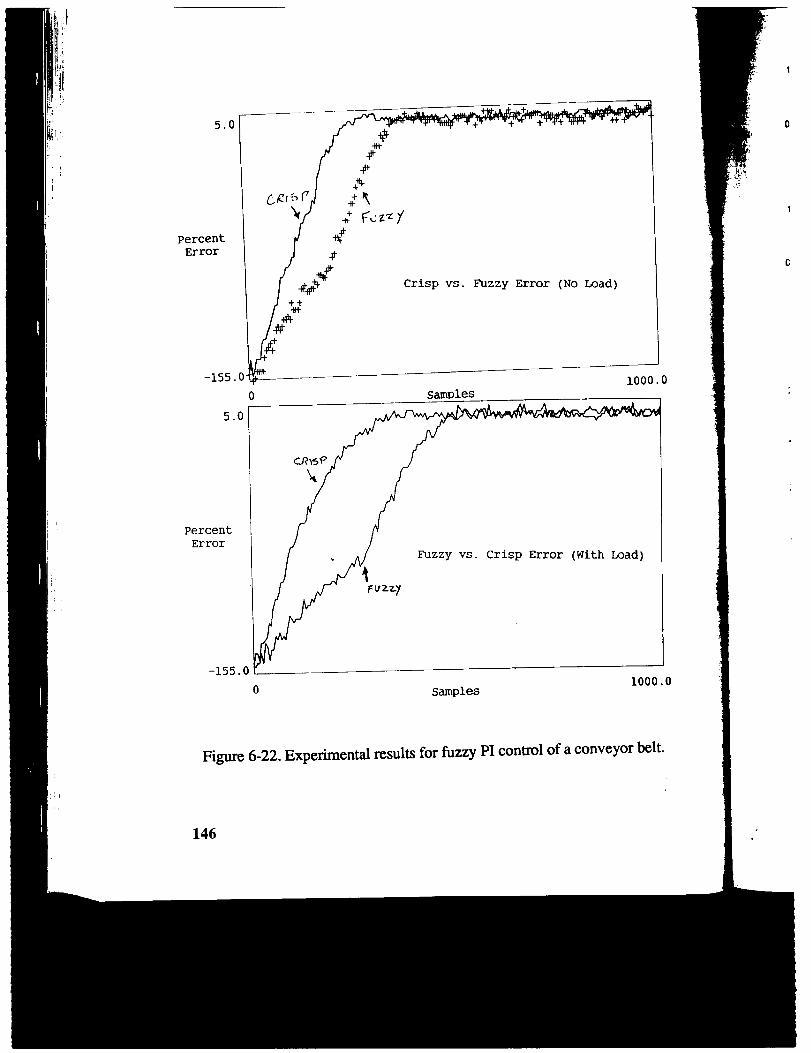
5.0
@15i’
\
percentError
Crisp vs. Fuzzy Error (No Load)
1000.00 samples
5.0
percentError
-155. (1000.0
0 samples
11
c
Figure 6-22. Experirnentd results for fuzzy PI control of a conveyor belt.
146

—
)00.0
)00
! ‘“;=1
JsH*
,, 00 60 100 160 200 250
Input Voltage
.~,
“,:
)elt.
1
0 1 1
0 50 100 150 200 250
260
240
220
200
180
160
140
120
Figure 6-23. Membtmhip functions for input/output voltages inSBFC experiment.
“donnloadlout” —
1
0 50 100 150 200 250 300
Figure 6-24. Software simulation for the input/output voltagesfor conveyor system.
147

—
I
Figure 625. Schematic of SBFC and conveyor system experimental set up.
2.4
2.2
2
1.8
,
,“ 1.4
1.2I
1
$4 +
I I 1 1
! o 0.5 1 1.5 2 2.5
Figure 6-26. Hardware result for conveyor system input/output voltages.j,,1:
,’ 148
M1
Fuzzya quadand Stithe fucha-acl

. up.
—o
~ *
—
2.5
,es.
7
A FUZZY TWO-AXISMIRROR CONTROLLER FOR
LASER BEAM ALIGNMENT
Richard D. MarchbanksUniversity of New Mexico
(Current address? Los Alamos National Laboratory, Los Alamos, NM 87545)
Fuzzy logic was used to control a two-axis mirror gimbal for aligning a laser beam usinga quadrant detector. A PC based controller was configured with a simple rule set to controland stabilize the device. A comparison between a non-fuzzy proportional controller andthe fuzzy controller was made. Experiments were performed to study the trackingcharacteristics and the effect of rule pruning on the fuzzy controller respnse.
149

150 Chap. 7 Fuzzy Laser Beam Alignment
7.1 INTRODUCTION
p The use of fuzzy logic is rapidly becoming a popular method of solving problems thatrequire a human-type response. Fuzzy logic uses sets of linguistic variables to solve
i problems where information is imprecise or a mathematical model of the system isI difficult to obtain. Fuzzy logic has many applications such as pattern recognition,
clustering, data fitting, diagnostics, and the most prevalent being control.
In the case of control, many systems are very nonlinear in nature and obtainingmodels of these systems are not only difficult but can be impossible. Many systems aredescribed by a linear model that approximates its behavior over a small region. For suchsystems, the model only works well in this small region. Outside this region, thesystems behavior can become unpredictable or unstable. By using of fuzzy logic, one caneasily realize such nonlinear systems without the requirement of a model.
7.2 PROBLEM FORMULATION
Communication systems are desired that use line-of-sight transmitting and receiving. Thisis especially true for submarine communication. A submarine requires the ability tocommunicate with other platforms but still remain “invisible.” A major requirement forsuch a system is the ability to maintain a communication link between platforms given avariety of disturbances such as movement, bumps, atmospheric or hydrosphericperturbations, and obstructions.
This chapter presents a demonstration of fuzzy control applied to such aproblem. It was an attempt to acquire educational experience in a fuzzy logic control andnot breakthrough research in solving the proposed problem Presented are the results ofwodt in a one semester graduate course in fuzzy logic control offered by the department ofElectrical Engineering and Computer Engineering at the University of New Mexico.
f’
7.3 APPROACH
A two-axis mirror gimbal is setup to sttxr a laser beam onto a quadrant detector wherethe beam spot is desired to lie on the center of the detector. Electronics sense the error inthe position of the beam relative to the center of the detector and produces two sigrudsrepresenting the x and y direction errors. ‘Ihese errons are convcmed to a digital format foruse by the personal computer driven fuzzy controller. The controller processes the errorinformation using fuzzy logic and chooses velocity signals for the motor driver. Thedriver supplies the required power to run the motors that repositions the beam. Figure 7-1outlines this closed-loop system.
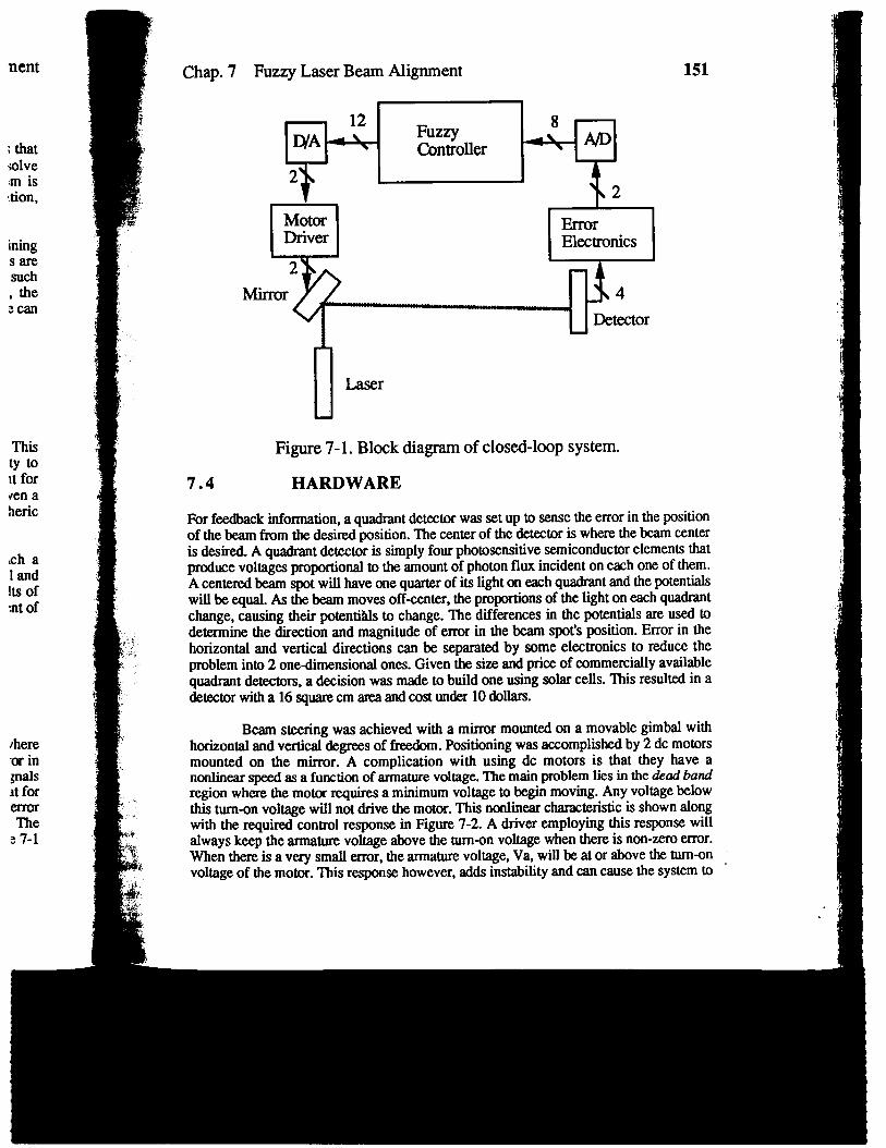
; thatmlve:m ismien,
inings aresuch, theL?can
Thisty toIt forvenaheric
,ch a1andIts ofmt of
m in,mals~tforerrorThe
27-1
Chap. 7 Fuzzy Laser Beam Alignment
FuzzyController
m
151
‘1 u Iktector
uLaser
Figure 7-1. Block diagramof closed-loopsystem.
7.4 HARDWARE
For feedback information,a quadrant detector was setup to sensethe error in the positionof the beam from the desired position. The center of the detector is where the beam centeris desired. A quadrant detector is simply four photosensitive semiconductor elements thatproduce voltages proportional to the amount of photon flux incident on each one of them.A centered beam spot will have one quarter of its light on each quadrant and the potentialswill be equal. As the beam moves off-center, the proportions of the light on each quadrantchange, causing their potentials to change. The differences in tie potentials are used todetermine the direction and magnitude of error in the beam spot’s position. Error in thehorizontal and vertical directions can be separated by some electronics to reduce theprobleminto 2 onedimensional ones. Given the size and price of commerciallyavailablequadrantdetectors,a decision was made to build one using solar cells. This resulted in adetector with a 16 square cm area and cost under 10 dollam.
Beam steering was achieved with a mirror mounted on a movable gimbal withhorizontal and vertical degrees of freedom. Positioning was accomplished by 2 dc motorsmounted on the mirror. A complication with using dc motors is that they have anonlinear speed as a function of armature voltage. ‘he main problem lies in the &ud bandregion where the motor requires a minimum voltage to begin moving. Any voltage belowthis turn-on voltage will not drive the motor. This nonlinear characteristic is shown alongwith the required conrrol response in Figure 7-2. A driver employing this response willalways keep the armature voltage above the turn-on voltage when there is non-zero error.When there is a very small error, the armature voltage, Va, will beat or above the turn-onvoltage of the motor. This response however, adds instability and can cause the system to

152 Chap. 7 Fuzzy Laser Beam Alignment
limit cycle when the error voltage is very small. Limit cycling is due to the very highslope of the control response curve near the origin; the motor switches between forwardand reveme directions. Part of the objective in the design was to rcdum or eliminate limitcycling with the fuzzy logic controller without the requirement of steppermotors.
speed Va
L1Va ErrorJ
\ Dead BandRegion
(a) (b)
Figure 7-2. a) Motor charaeteristic~ b) Desired anrtature voltage response.
The controller was employed using a PC with a 386 microprocessor. AKeithley-Metrabyte 8-bit analog-to-digital converter was used to put the analog error inthe digital format required by the computer. The input of the A/D converter has a rangefrom –5 volts to 5 volts with a resolution of 8-bits over this range. The error signal wasconditioned with amplifiers to fill this range and acquire the full 8-bit resolution. Afterprocessing, the resulting digital response signal was converted to an analog voltage fordriving the motors by a Keithley-Metrabyte 12-bit digital-to-analog converter.
7.5 SOFTWARE
Designing the required software to perform fuzzy inference can be a very involving taskbut fortunately there are a few packages that have been written to do this. One of thesepackaga, Togai InfraL@c Fuzzy C, was used to write the primary code that performedthe fuzzy arithmetic. This software is programmed in a language developed by themanufacturer that allows the user to easily construct a subroutine containing membershipfunctions and a rule base. The resulting code is compiled into C by a special compiler.The compiled subroutine performs all the required fuzzy operations, includingdefuzzification, and produces a crisp output. A driver program was written tocommunicate with the AVDand D/A converters and the fuzzy subroutine. It also was usedto acquire data from experiments. Listings of the Fuzzy C code, the A./D and D/Aconverter addresses, and driver program are listed in appendices A, B, and C re-spctively.
To represent the error input to the controller, a set of linguistic variables waschosen to represent 5 degrees of error, 3 degrees of change in error, and 5 degrees ofarmature voltage. Membership functions were constructed to represent the input and
Chap
Outpufuncti
Errc
DE
kVc

—
,-ent
:ry highforwardue limit
onse.
ser. A:rror inI rangelid was. Afterlge for
lg taskf theseOrmedby theErshipnpiler.Iudingten to.s usedi D/A~ely.
:s wascm ofIt and
Chap. 7 Fuzzy Laser Beam Alignment 153
output values’ degrees of truth for each of these linguistic variables. llese membershipfunctions are shown in F@re 7-3.
NS ZE PS PM
Error
volts-5 -.8 101 .8 5
-,2J ‘.2(a)
NS ZE Ps
DEITOI
volts
-2 6 0 .6 2-.(b)
NS m Ps PM
ArmatureVoltage
volts-lo -5 0 5 10
(c)
Whm NM= “negative medium”
NS = “negativesmall”ZE = “m”Ps= “positive small”PM = “positive medium”
Figure 7-3. Membership functions. a) Input error,b) Input change in error, c) Output armature voltage.
The input error membership functions contain a very narrow zero error (ZE)region. A faster convergence was expected by doing this because for a small error, the

154 Chap. 7 FUZZYLaser Beam Mignment
degree of “medium” will be large and the armature voltage will correspondingly be largerthan if ZE were broad. Also, the ‘medium” membership functions for both the error andarmature voltage were chosen not to intersect at zero. This was done to help supprewiovershoot and limit cycling. because the motors response was equal in the forward andreverse directions, the membership functions were made with a symmetry about zero.
;: Here is one of the advantages of fuzzy logic. If the motors response functions are;asymmetrical, having a different response in the forward direction than the reversedirection, the memtwship fimctions can be designed to make the response act as thoughthe motors functions have symmerncal responses.
Two sets of rules were chosen. These “Fuzzy Associative Memories” or FAMs,are a shorthand matrix notation for presenting the rule set. A linguistic armature voltagerule is fwed for each pair of linguistic error variables and linguistic change in errorvariables. For example, if the error is PM and the change in error is ZE then the armaturevoltage is NM. Because overlap between the fuzzy variables exis~ more than one rule canfm simultaneously.
A set of “pruned” rules was used to investigate the effect of reducing theprocessed information on the controller’s behavior. When pruned, the FAM was slightlymodified to incorporate all the rules. Note that the FAM banks, like the membershipfunctions, are also symmetrical. The effect on the system’s response by modifying theFAM bank is more dramatic than modifying the membership functions. Changing theFAM “coarsely” tunes the response while adjusting the membership functions “finely”tunes the response.
The FAMs are shown in Figure 7-4. Figure 74a shows the full set of 15 rules.Figure 7-4b shows the set after pruning.
Error
m
NM NS ZE PS PM
PM PM PS ZE NS
PM PS ZE NS NM AError
PS ZE NS NM NM
(a)
NS
ZE
Ps
Error
%
NM NS ZE PS PM
Ps ZE
PM ZE NM
ZE NS
(b)
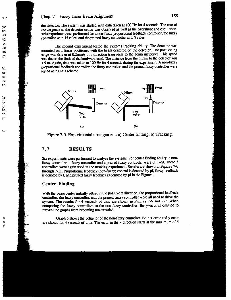
mt
;andSsId‘o.re
se
~h
fs,georrean
heIyiphenev“
s.
n
t:
Chap.7 Fuzzy Laser Beam Mi~ent 155
the de~mr. The system was started with data takenat 100Hz for 4 seconds.The rate ofconvergenceto the deteztorcenter was observedas wellas the overshootand oscillation.‘rltii experimentwas performedfor a non-fuzzyproportionalfeedbackcontroller,the fuzzycontrollerwith 15rules, and the prunedfuzzycontrollerwith 7 rules.
The second experiment tested the systems tracking ability. The detector wasmounted on a linear positioner with the beam centeredon the detector.me positioningstage was drivcmat 0.2mm/s in a direction transverseto the beam incidence.This speedwasdue to the limit of the hardwareused.‘l%edistancefromthe mirrorto the detectorwas1.5m. Again,data was takenat 100Hz for4 secondsduring the experiment.A non-fuzzyproportionalfeedback controller, the fuzzy controller, and the pruned fuzzy controller weretested using this scheme.
(a) 0)
Figure 7-5. Experimental arrangement: a) Center finding, b) Tracking,
7.7 RESULTS
Six experimen~ were performed to analyze the systems. For centerfinding ability, a non-fuzzy controller, a fuzzy controller and a pruned fuzzy controller were utilized. These 3controllers were again used in the tracking experiment. Results are shown in Fi- 7-6through 7-11. Proportional feedbxk (non-fuzzy) control is denoted by pf, fuzzy feedbackis denoted by f, and pruned fuzzy feedback is denoted by pf in the FQures.
Center Finding
With the beam cemtexinitially offset in the positive x direction, the proportional feedbackcontroller, the fuzzy controller, and the pruned fuzzy controller were all used to drive thesystem. The results for 4 seconds of time are shown in Figures 7-6 and 7-7. Whencomparing the fuzzy controllers to the non-fi,uzy controller, the y-error is omitted toprevent the graphs horn becoming too crowded.
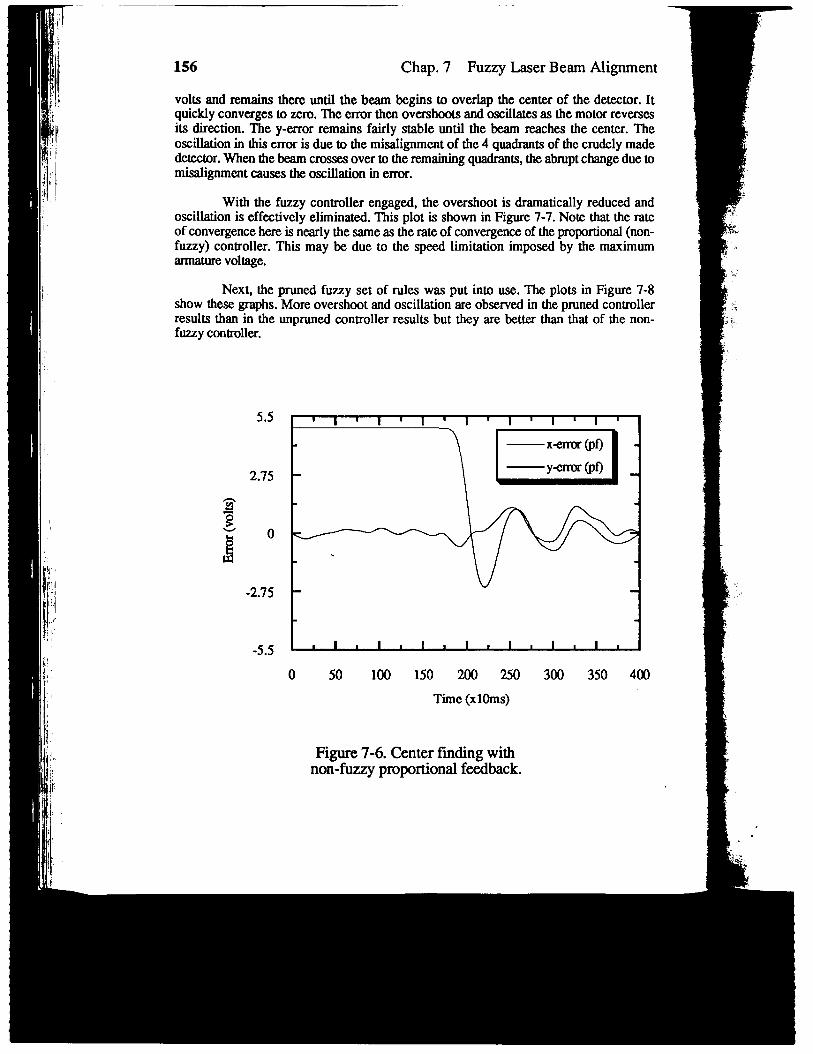
156 Chap. 7 Fuzzy Laser Beam Alignment
volts and remains there until the beam begins to overlap the center of the detector. Itquickly converges to zero. The error then overshoots and oscillates as the motor reversesits direction. The y-error remains fairly stable until the beam reaches the center. Theoscillation in this error is due to the misalignment of the 4 quadrants of the crudely madedetector. When the beam crosses over to the remaining quadrants, the abrupt change due tomisalignment causes the oscillation in error.
With the fuzzy controller engaged, the overshoot is dramatically reduced andoscillation is effectively eliminated. This plot is shown in Figure 7-7. Note that the rateof convergence here is nearly the same as rhe rate of convergence of the proportional (non-fuzzy) controller. This may ~ due to the speed limitation imposed by the maximumarmature voltage.
Next, the pruned fuzzy set of rules was put into use. The plots in Figure 7-8show these graphs. More overshoot and oscillation are observed in the pruned controllerresults than in the unp~ned ~ntroller results but they are better than that of the non-fuzzy controller.
5.5
2.75
0
-2.75
-5.5
m I 1 I 1 I n I 1 I 1 I 1 1 1
\ EELJ
.
I 9 1 1 1 1 I n 1 n 1 1 1 1 1 n I
o 50 100 150 200 250 300 350 400
Time (xlOms)
Figure 7-6. Center finding withnon-fuzzy proportional feedback.
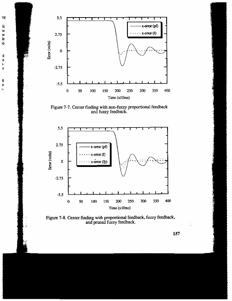
Int j
It ‘%Ie
le
!O
d.e1-n
8xi-
1
5.5
2.75
z~w
~
0
-2.75
-5.5 m 1 1 1 1 1 1 I m 1 n I m 1 t
0 50 100 150 200 250 300 350 400 !Time (xlOms) !
Figure 7-7. Center finding with non-fuzzy proportional feedbackand fuzzy feedback. 4
5.5 r n I m I I I 1 1 m I 1 1 n [ n I
2.75
0
-2.75
— x-error @f)
----- x-em (f)
. . . . . X-aor (fp)
o 50 100 150 200 250 300
1
;,350 400
Time (xloms)
Figure 7-8. Center finding with proportional feedback, fuzzy feedback,and pruned fuzzy feedback. d,.

.
158 Chap. 7 Fuzzy Laser Beam Alignment
Tracking
The second set of experiments was performed to examine the tracking ability of thecontrollers. With the beam centered in the desired position, the detector was set intomotion and the controllers engaged. Data was taken as in the previous experiment and isshown in Figures 7-9 through 7-11. The non-fuzzy controller shows substantialoscillation in both the x-error and y-error as shown in Figure 7-9.
Figure 7-10 shows the results of the fuzzy controller x-error along with the non-fuzzy controller x-error. The fuzzy controller reduces the oscillation but a slight offset isobserved. This indicates that the fhzzy controller lags slightly behind the detector.
Finally, the pruned fuzzy controller is tested. As in the center-finding test, thepruned set does not reduce the oscillation as well as the full fuzzy set. However, it doesperform better than the non-fuzzy controller in this respxx. A slight offset was alsoobserved here.
1 1 [ 1 I 1 I m I n I 1 I I 1 1
0.6 ..-,~.. . . -- .,-~,./-., --
s,
~w
EI.u -0.2
.
-0.6
-1 1 1 n 1 1
0 50 100 150 200 250 300 350 4(X)
Time (xlOms)
Figure 7-9. Tracking with non-fuzzy proportional feedback.

lent
theinto
d istial
on-:t is
theCMho
x)
‘i
Iv—
h
.,. k -0.2
-0.6
1 3w Ii --------,,,, ‘g
{——_’_”~-0.2 ‘ -------------------
.’
-~ ~
o 50 100 150 200 250 300 350 4m
Time (xlOms)
Figure 7-10. Tracking with non-fuzzy proportional feedbackand fuzzy feedback.
1 , I , I 1 I m 1 1 1 11
E[
,
0.6
n --------___ ------- ----- ----- -,- ”--- *
— x-error(@3
----- xaror(f)
. . . . . x-error(m)
0 50 100 150 200 250 300 350 4m
:. Time (xlOms)~,:
~.,? Figure 7-11. Tracking with proportional feedback, fuzzy feedback, and
I
“,$,.. pruned fuzzy feedback.
‘:1} 159i ...

160 Chap.7 Fuzzy
7.8 CONCLUS1ONS
.aser Beam Alignment
By implementing fuzzy control in this tracking system, overshoot was significantlyreduced and limit cycling was virtually eliminated However, justification of the addedcomplexity of the micro-controller cannot be accomplished until a comparison is madewith conventional proportion.al-plus-in~gral (PI) control and propordonal-plusderivative(PD) control. These Esu.lm simply show the ease of implementation of fuzzy control to aproblem without using a mathematical model of the system. Future study should beconsidered in modeling the system and implementing PI and PD controllers to furtherestablish or dispute the viability of fhzzy control for this particular problem.
Additional possibilities include reducing the amount of hardware. The errorelectronics and nonlinear motor driver circuit can be removed and replaced by the fuzzycontroller. Further work can lead to a more optimum set of membership function andrules. Perhaps methods of designing the membership functions could be explored such astechniques described by Wang and Mendel.
ACKNOWLEDGMENTS
Special thanks to Renee Temple who helped me through the tough times by teaching meC, to Denis Barak for help with A/D and D/A processes, and to the Chemical and LaserSciences Division at Los Alamos who loaned me some equipment that made this projectpossible. And of course to Dr. Mo Jamshidi, who gave me motivation to accomplish thisgoal.
REFERENCES
[1]
[2]
[3]
[4]
[a
Klir, G. J., and Folger, T. A. ( 1988). Fuzzy Sets, Uncertainty, and Information,Prentice-Hall.
KOSICO,B. (1992). Neurai Networks and Fuzzy Systems: A Dynamical SystemsApproach To Machine Intelligence, Prentice-Hall.
Phillips, C. L., and Harbor, R. D. (1988). Feedback Conlrol Sysrems, Prentice-Hall.
Wang, L. Mended, J. M. Generating Fuzzy Rules From Numerical Data, WithApplications, USC-SIPI Report #169
Zadeh, L. A. “Knowledge Representation in Fuzzy Logic,” IEEE Transactions onKnowledge and Data E~gineering, Vol. 1, No. l,-Mar~h 1989.
Cha
AP
I*
*/
PI

nent
ntlyldedladetivetoaI bether
norIZzyandIas
melserjectthis
*
1
Chap. 7 Fuzzy Laser Beam Alignment161
APPENDIX A
I*Laser Beam Alignment Fuzzy Inference EngineWritten using Togai InfraLogic Fuzzy C Software
*J
PROJECI’ Alignment
/* Error of the spot measured in 0.039 volts.* The universe of discourse is [-5.0, 5.0] volts.*J
VAR Error$YE s&ed byte
W- 127
/*C type of ‘signed char’ *//* universe of discourse min *//* universe of discourse max */
/* Membership functions for Enor (ZE, PS, NS, PM, NM). */
MEMBER ZEPOINTS -20001200
END
MEMBER PSPOINTS 302011270
MEMBER NSPOINTS -1280-201-30
MEMBER PMPOINTS 20010011271
MEMBERNMPOINTS -1281-1001-200
END /* end of Error definition*/
/* dError, the velocity of the spot (or detector),* meas~~ in vol~. The universe of discourse
* [-2,2] volts/second.

‘1
162 Chap. 7 Fuzzy Laser Beam Alignmentt
*/
VAR dErrorTYPE signed byte /*C type of ‘signed char’ */
( MIN-loo /* universe of discourse min*/
MAx 1(XI /* universe of discourse max*J
/* Membership functions for dEmor (ZE, PS, NS). */
APPENDIX A
MEMBERZEPOINTS-30001300
MEMBER PSPOINTS OO3O11OO1
MEMBER NSPorNTs -1001-30100
END /* end of dError definition */
/* Armature voltage of motor in .078 volt increments* The universe of discourse is [-128,127] *.078 volts.*/ .
VAR SpeedTYPE signed byte /*C type of ‘signed char’ */MIN -128 /* universe of discourse min */MAX 127 /* universe of discourse max
*/
/“ Membership functions for Speed (ZE, PS, NS, PM, NM). */
MEMBER ZEPOINTS-50001500
MEMBER PSPOINTS 515011270
END

Chap. 7 Fuzzy Laser Beam Alignment
MEMBER NSPOINTS -1280-501-50
MEMBER PMPOINTS 50012511271
MEMBERNMPOINTS -1281-1251-500
END /* end of Speed definition*/
/* Rules for response*/
FUZZY Alignment_rules
RULE RulelIF Error IS PM AND dError IS ZE THEN
Speed IS NMEND
RULE Rule2IF Error IS PS AND dError IS PS THEN
Speed IS NMEND
RULE Rule3 .
IF Error IS PS AND dError IS NS THENSpeed IS ZE
RULE Rule4IF Error IS NM AND dError IS ZE THEN
Speed IS PMEND
RULE Rule5IF Error IS NS AND dError IS NS THEN
Speed IS PM
163

164 Chap. 7 Fuzzy Laser Beam Alignment
RULE Rule6IF Error IS NS AND dError IS PS THEN
Speed IS ZE
RULE Rule7IF Error IS ZE AND dError IS ZE THEN
Speed IS ZE
RULE Rule8IF Error IS ZEANDdError IS NSTHEN
Speed IS PS
RULE Rule9IF Error IS ZE AND dError IS PS THEN
Speed IS NS
RULE Rule lOIF Error IS NS AND dError IS ZE THEN
Speed IS PSEND
RULE Rulel 1IF Error IS PS AND dError IS ~ THEN
Speed IS NS
RULE Rule12IF Error IS NM AND dError IS NS THEN
Speed IS PM
RULE Rule13IF Error IS NM AND dEmor IS PS THEN
Speed IS PS
RULE Rule14

W
Chap. 7 Fuzzy Laser Beam Alignment
RULE Rule15IF Error IS PM AND dError IS PS THEN
Speed IS NM
END /* end of knowledge base*/
/* The following three CONNECT Objects specify that Error* and dError are inputs to the Alignment.rules knowledge base* and Speed output from Alignment_rules.*I
CONNECTFROM ErrorTO Alignrnent_rules
END
CONNECI’FROM dErrorTO Alignment_rules
END
CONNECTFROM Alignment_rulesTo Spxd
END
END
●
165
,;*..,
i‘,

‘i1
I
166 Chap. 7 Fuzzy Laser Beam Alignment
APPENDIX B
/*
address.h
Defined constants representing the addresses and maskinginputs for the A/D and D/A converters.
*I
#include <stdlib.h>#include estdio.h>#include etilcomp.b
#define atod_strt OX0200 /* A/D base address. */#define atod.data OX0201 /* A/D data address (base+ 1).*/#klefme atod_ctrl OX0202 /* A/D control address(base+ 2).*/#define atod_statOX0203 /* A/D status address (base+ 3).*/
#define dtoaO_loc OX0208 /* D/A ch~nel O address, */
#define dtoal_loc Ox020a /* D/A ch~nel 1 address.*/
#define disable_5_ints OX05 /* Disable A/D channel 5 ext.interupts. */#define disable_7_ints OX07 ~ Disable A/D channel 7 ext.interupts. */#define masking_eofc 0x80 /* s~~s chWk of end of data
conversion. */
.

lent
I
‘/
m
Chap. 7 Fuzzy Laser Beam Alignment
APPENDIX C
I*Fuzzy Laser Beam Tracker driver progmmRichard MamhbanksLos Alamos National Laboratory
*/
#include “address.h”#include “stdio.h”
rnaino{
~ Global Data Variables.*/char S&tUS;int err_x,emfl;int dxem,dyem,int xerr, yer,int xerr_old, yem_old;int Error, dError, Sped,int i, j, s;
P Data Storage.*/float x_data[500]; p x sampled data*/float y_data[500]; /* ysarnpled data */char datafile[15]; /*storage of sampled data*/FILE *@;
F Initialization.*/i=O, .
;:?. /* sample rate*/
dxem’= Qdyerr = mxerr_old = ~yerr_old = Q
printf(’NhFUZZY BEAM ALIGNMENT”);
printf(’%kPlease enter filename”);scanf(’’%s”, datafile);
pMtf(’b.Progmm Executing: Press a key to quit.”);
/* While the keyboard is not pressed, execute program.*/
167

168 Chap. 7 Fuzzy Laser Beam Alignment
~hile(kbhito == O)
/* X-ERROR*/
/* Disable interrupt.*/outportb(atod_ctrl, disable_5_ints);
P start a/d conversion*/outportb(atod_strt, 1);
/* wait until conversion complete*/while( (status=inportb(atod_stat) & maskin~eofc) != O );
F mad the dam*/err_x = inportb(atod_data);
/* Y-ERROR*/
~ Disable interrupt. */outportb(atod_ctrl, disable_7_ints);
/* start rdd conversion */outportb(atod_strt, 1);
p wait until conversion complete*/while( (status=inportb(atod_swt) & masking_eofc) != O);
F read the data*/em_y = inportb(atod_data);
.
p Write data to array every sth data value.*//*Do this for 500 data values and stop saving them*/
if ((i ==s-l)&&(jc=499)) /* sample everys time*/
(x_dataU] = (em_x - 128) * .039;y_datati] = (ems - 128)* .039;i=O,j++,
)“
elsei++,

Chap. 7 Fuzzy Laser Beam Alignment
/* Put the data in signed byte form form for fuzzycOntrollerW
xerr = err_x - 128;yerr = err_y - 128;
/* Find delta errors*/
dxerr = xerr - xerr_old;dyerr = yerr - yerr_old;
/* Update old errors*/
xerr_old = xernyerr_old = yem,
~ Call fuzzy ties *I
Alignment(xerr, dxerr*2, &Speed);
err_x = Speed+l 28;
Alignment(yen, dyti2, &Spe~);
err_y = Speed+128;
/* Write to channel OD/A*/err_x = (err_x e< 8);outport(dtoaO_loc, err_x );
/* Write to”channel 1 D/A */err~ = (err_y << 8);outport(dtoal_loc, err_y );
)
printf(’’khd%ogram Terminated:”);printf(’hkWriting data to fde: %s”, data.file);
fp = fopen(datille, “w”);
Wntf(m, “m= BEAM ~~w%R~,~M~”);fprintf(fp, “X-ERROR - ;
for (i= Q i<= 499; i++)
169

H!1‘:170 Chap.7 Fuzzy Laser Beam Aligntnent
(
fprintf(fp, “%f %fM”, x_data[i], y_data[i]);)
fclose(fp);
printf(’~tiile Transfer Complete.hh”);)/* end of driver program*/ m

SIMULATION OF TRAFFIC
r
FLOW AND CONTROLUSING FUZZY AND$
CONVENTIONAL METHODS
12
Robert L. KelseyKeith R. Bisset
X-g, Los Alamos National Laboratory
12.1 INTRODUCTION
Fuzzy logic can be used as an alternative method for the controlof trafficenvironments.A traffic environment includes the lanes to and from an intersection, the intersection,vehicle traffic, and signal lights in the intersection. To test the fuzzy logic controller acomputer simulation was constructed to model a traffic environment. A typical crossintersection was chosen for the tmffic environment and the performance of the fuzzy logiccontroller was compared with the performance of two different types of conventionalcontrol. The fuzzy logic controller proved to be a better method of control thanconventional conirol methods es~ially in the case of highly uneven traffic flow behveenthe different directions.

2
cLDs
‘Y?t
Y
s.1,
a;s
:n
1
263
~
~
(
Chap.12 Fuzzy Tra.i31cControl
12.2 TRAFFIC CONTROL METHODS
There are two types of conventional control. One type of control uses a preset cycle timeto change lights. The other type of control combines ptesel cycle times with proximitysensors which can activate a change in the cycle time or the lights. In the case of a lesstraveled street which may not need a regular cycle of green lights, a proximity sensor willactivate a change in the light when cars are present. This type of control depends onhaving some prior knowledge of traffic flow patterns in the intersection so that signal
‘?&cycle times and placement of proximity sensors may lx customized for the intersection.
..!L,. Fuzzy logic control is an alternative to conventional control which can control a... wider array of traffic patterns at an intersection. A fuzzy-controlled signal light uses
sensors that count cars instead of proximity sensors which only indicate the presenm of
k cars. This provides the controller with traffic densities in the lanes and allows a better,-. assessment of changing traffic patterns. As traffic disrnbutions fluctuate, the fuzzy,,.’, controller can change the signal light accordingly.,,
12.3 SIMULATION.,,’,.The eomputcr simulation was written in the C++ computer programming language usingobject-oriented programming techniques. Object-oriented programming allows thesimulation to be built in a modular fashion making it both expandable and easilymaintainable. Thus, new features are easily added to fie simulation and current featur&can be modified with little impact on the rest of the program.
The graphics portion of the simulation was written using the X Window Systemas described by Nye (1988, 1991) and Young (1989), specifically the Xt Intrinsic libraryand the Athena (XaW)and Hewlett-Packard (XW)widget libraries, collectively called the XToolkit. The use of the X Toolkit provides a set of widgets which ean be combinedtogether to create the simulation. A widget is a graphical object such as a button or aslider. Their use allows the low-level graphical details to be ignored
.The X Toolkit (and X Windows in general) is event driven. The simulation
respondsto events, such as a button press, generated by the user. Any one of a number ofactions can be performed at any time which greatly enhances the interactive nature of thesimulation.
+,’,( 12.3.1 Vehicle Movement“4
The crux of the simulation problem is the modeling of traffic flow to mimic reality,,=specifically the motion of the vehicles relative to one another. Physical equations were
I used to describe the motion of a car based on the car immediately in front of it (theleading car). J@uuion 1 describes the acceleration of a car based on the vekwities and
,i
5
positions of the car and the leading car. This equation is a time-delay differential equation
!
which comes horn traffic flow theory presented by Haight (1%3), Montrol (1961), andMorris (1%7). Equations 2 and 3 are standard classical physics equations for the velocityand position of an object based on the object’s acceleration. v (t) and X(t) are the velocity
~., and position, respectively, of the car at time t,while v’(r) and x’(t) are the velocity and “

1
~position of the leading car. t is the driver reaction time and Vfreeis the & velocity ofthe car (the velocity at whichthe car woulddrive withoutinterferencefromothercars).
v(t) = v(t- 1) + a(t)dl (2)fl~
x(f) = X(t-1) + V(t)df + ~(?)dz (3)L
The free velocity of each car is mndomly set from a normal distribution with amean of the “posted” speed limit in the lane. As observed in reality, this provides thesimulation with cars which drive the speed limit and cars which drive faster and slowerthan the speed limit. The driver reaction time, z, is the time expended when a driver sees a
disturbance, the brain processes the information, and the driver takes an appropriateaction. lhis time is equal to one and one half seconds.
12.3.2 In~ut
[
.
The simulation has a variety of modes and other configuration inputs which may be,’ selected from an input file when the program is executed. These inputs inclu& the type of
controller (timed, proximity, or fuzzy) which may be used to control the traffic signal,
1whether to use graphics or batch mode, flow rates, percentage of turning cars, and how
;/, long (in simulation time) the simulation should run.
1~ Flow rate in cars per hour may ke specified sepamtely for each of the four lanes.i,1. This parameter may be either a single value (cars per hour) or a series of flow-time pairs?>\ (two numbers: flow and time). If a single value is given then that flow rate is used for the
entire simulation run. The cars are actually generated and entered into the simulationrandomly to obtain the s@fkl flow rote, but to make the flow pattern or disrnbution of
I
cars more nonuniform. The flow-time pairs give the flow rate at certain times during thesimulation run. The simulation interpolates between these pairs to provide a smooth
I transition between flows. Flow-time pair inputs are useful for determining how thecontroller will perform in a given intersection over the course of an entire day, or someother time period. A sample input file that uses both flow-time pairs and single values isIshown in Ap~ndix A.
12.3.3 Operating Mode
The simulation has two operating modes. A graphics mode displays a scaled trafficenvironment and a batch mode executes without graphics. The graphics mode animatesthe movement of cars in lanes directed to and from the intersection. Also displayed arestatistics about the cars which have moved through the trafilc environment. llese includeflow rate (cars per hour), average waiting time, and average driving time. The averagewaiting time in seconds is an average of the time all cars spend at zero velocity in thesimtdation. The average driving time is the average of the time all cars (completing the

;ontrol
city ofrs).
(1)
(2)
(3)
with aIes theslowerseesa
)priate
lay beype ofsignal,d how
lanes.: pairs
‘or theIationion ofIg thenoothw thesomeues is
raffic
natesd areeludexagen theg the
Chap.12 Fuzzy Traffic Control 265!,.
. . . . . . . . . . . . . . . . . . . . . . . .
#
Figure 12-1. Cross Intersection.
simulation)spend at a velocity greater than zero during the executionof the simulation.In addition, the fuzzy controllervemion of the ~phics simulationhas “popup” windowsavailablewhich display the degree of memlxxship (refex to Section 12.4.1) for each of theinputs, which fuzzy rules are king f~, and a list of the fuzzy rules. This informationgives insight into the workings of the fuzzy controller.
The graphics mode also allows certain inputs originally set in the input fde tobe changed intmctively. These inputs include the flow rate in each direction and the cycletime length of the lights. Due to tie computational overhead of generating graphics, thebatch mode can execute as much as En times fasterthan the graphics mode. This makesthe batch mode ideal for running exhaustive tests using different traffic patterns for thethree differentcontrollers.
12.3.4 Evaluation Function
The statisticsgeneratedby the simulationare usd to calculatea cost function(equation4)as a means of evaluatingthe performanceof the fuzzy controlleragainstthe conventionalcontrollers. Waitman is the ave~ge waiting time. Driveman is the average drive time.Carsout and Carsinarethe number of cars exiting and entering the traffic environment,respectively, while k is a constant which is equal to 100. The lower the cost function, thebetter the pxformance.
cost = Wait~
k()
CarS.U DriVe~Cars~
(4)
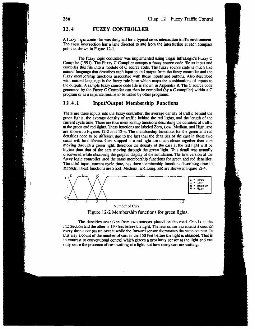
12.4 FUZZY CONTROLLER
A fuzzy logic controller was designed for a typical cross intersection traffic environment.+The cross intersection has a lane directed to and from the intersection at each compasspoint as shown in Figure 12-1.
The fimy logic controller was implemented using Togai Infrabgic’s Fuzzy CCompiler (1991). The Fuzzy C Compiler accepts a fuzzy source code file as input and
f compiles this file into a module of C source code. The fuzzy source code is much likei natural language that describes each input to and output from the fuzzy controller and the
Ifuzzy membership functions associated with those inputs and outputs. Also describedwith natural language is the fuzzy rule base which maps the combinations of inputs tothe outputs. A sample fuzzy source code file is shown in Appendix B. The C source code
1 generated by the Fuzzy C Compiler can then be compiled (by a C compiler) within a Cprogram or as a separate routine to be cdlcd by other programs.
12.4.1 Input/Output Membership Functions
~
,,
There are three inputs into the fuzzy controller, the average density of traffic behind thej green lights, the average density of traffic behind the red lights, and the length of the
current cycle time. There are four membership functions describing the densities of trafllcat the green and rcd lights. ‘Ik.se- functions are labeled Zero, Low, Medium, and High, andare shown in Figures 12-2 and 12-3. The membership functions for the green and rd
3,densities need to be different due to the fact that the densities of the cars in those two
\cases will be different. Cars stopped at a red light are much closer together than cars
Imoving through a green light, therefore the density of the cars at the red light will be
ihigher than that of the cars moving through the green light. This detail was actuallydiscovered while observing the graphic display of the simulation. The fmt version of the\fuzzy logic controller used the same membership functions for green and red densities.
$
k
The third input, current cycle time, has three membership functions describing time inI;‘L seconds. These functions are Short, Medium, and Long, and are shown in F@re 12-4.
H. . Z--L-N”>
Number of C.ws
Figure 12-2 Membership functions for green lights.
The densities are taken from two sensors placed on the road. One is at theintersection and the other is 150 feet before the light. The rear sensor increments a counterevery time a car passes over it while the fmward sensor decrements the same counter. Inthis way a count of the nurrdm of cars in the 150 feet &fom the light is obtained. This is ~
i
in contrast to conventional ~ntrol which places a proximity sensor at the light and can Ionly sense the presence of cars waiting at a light, not how many cars are waiting. i

31
L.s
.
i3.i)3.
::.iI)i
1
Chap. 12 Fuzzy Tra.flit Control 267
T,1
H
n
Z = ZeroL= LowM = MediumH = High
o01 3 6 9 12
Number of Cars
Figure 12-3. Membershipfunctions for red lights.s
1M L
o
S - ShortM - MediumL- Long
n“ o 30 60 90 110
~ime (seconds)
Figure 12-4. Membership functions for time.
N1
P M P
~n
YN -NoPN - Probably Not4- MaybePY - Probably YesY = Yes
00 0.1 0,2 0.3
Degree of Change
Figure 12-5. Membership functions for change.
The outputof the fuzzycontrollerdecideswhetherto changethe stateof the light(for example, green north-south to -n east-west) or remain in the same state, The
j~, membershipfimctionsfor change are No, Probably No, Maybe,Probably Yes, and Yes.,:,<llese functionsrepresenta degr~ (fuzzyvalue)of a binaryvalue, 1beingyesand Obeingno, and are shownin Figure 12-5. I
Other attempts at fuzzy control of traffic signals, particularly by Gallegos(1991), have used the fuzzy con~oller to make incremental changes in the times of the
+ cycle in each direction, We rejected that approach because it was felt that a controllerwhich could make immediate changes to the light based on the current conditions waspreferable.
12.4.2 Fuzzy Rule Base“i: 1
.,,.? The fuzzy rule base maps the combination of the inputs to the output to decide whether to“
change the light. In the fuzzy source code file the fuzzy rule base is a list of if/then .+ statements. The number of rules is qllal tO the number of input combinations derived
JQ

268 Chap.12 FuzzyTrafficConmol
fim thenumberofmembershipfunctimsperinput.For example, if there are two inputseach having three membership functions, then the number of rules would equal nine.
It is possible to scale down the number of fuzzy rules when certain inputcombinationsare unnecessary.‘l%efuzzytrafficcontrollerdesignpresentedwouldyieldarule base of 48 rules, but for certain combinations the input for cycle time has nomeaning. For example, when the green traffic density is zero and the red traffic density iszero then the input for time does not matter. The desired output (change) is the same forany amount of time. Thus, one rule takes the place of three rules. The fuzzy controllerpresented uses 26 different fuzzy rules as shown in Appendix C.
12.5 TESTING AND RESULTS
Testing of the fuzzy controller involved the simulation of 625 different parameter sets.These parameter sets vary the flow of traffic in each of four lanes, from Oto 1200 cars perhour, with an increment of 300 (hence, 625 combinations). Each of these parameter setsis simulated for one hour of simulation time and generate statistics including the averageflow rate (cars/hour), average driving time, and average waiting time. Results, in the formof the statistics, of the fuzzy controller simulations are compared with the same 625parameter sets using a conventional controller (cycle time controller). Overall, the fuzzycontroller shows a modest increase in average flow rate. In particular, when trafficdensities are highly uneven, the fuzzy controller shows a substantial increase in averageflow rate. More significan~ perhaps, themthe average flow rate is the comparkm of theaverage waiting time. For the fuzzy controller, the average waiting time decreased by 49percent when compared with the conventional controller.
Another parameter file was constructed to simulate a “day in the life” of a trafficsignal. The objective was to simulate and observe how well the fuzzy controller handledtraffic during the span of a 12 hour day. The cross intersection was used to represent atypical city intersection with the north-south direction being a main artery and the east-west direction being a feeder artery. The 12 hour day included morning rush time,morning lull, lunch rush time, afternoon lull, school’s out rush time, and evening rushtime. Again, the fuzzy-controller simulation was compared with conventional-controllersimulation. The fuzzy controller handled ten percent more cars than the conventionalcontroller. The fuzzy controller also showed an eight percent increase in avexage flow rate,a 64 percent decrease in average waiting time, and a 29 percent decrease in the maximumwaiting time. Figure 12-6 shows the flow mtes throughout the 12 hour day. North-southand east-west flow rates are represented. Figure 12-7 shows a performance comparison ofthe fuzzy controller with two different conventional controllers across the 12 hoursimulation. One conventional controller is the cycle time controller and the other is acycle time controlled enhanced with proximity sensors (refer to Section 12-5.2 AdditionalTesting).
The 625 different combinations simulations were useful in identifying strengthsand weaknesses in the fuzzy controller. Using this information, we were able to modifyaspects of the fuzzy controller and improve its performance. The “day in the life”simulation and the corresponding results are more interesting because they provide a “real
(

Control
JOinputsne.
in inputd yield ahasnoensity isarne formtroller
:ter sets.am pereter setsaveragehe formme 625le fuzzy1 trafficaveragen of thed by 49
a traffichandledresent ahe east-h time,ng rushntrollermtional)Wrate,~imumh-southison of2 hourler is aiitional
rengths
modify
e life”a “real
1200
:000
cars600
400
20C
(
North-SOuth —Eamc-W=SC ‘-.
o 6C lao 240 300 ?460 420 480 540 600 660i20
0.03
c. 025
0.02
cost 0.015
llrne (minutes)
Figure 12-6.12 hour flow rates.
Fuzzy —
Proximity ––.
Timed ‘--
. . . . .
,’ ‘. .,’! -.. --.1,,, , -. \,
,-;i ,
i’ \,, ,, (s1’,, 1,
1:
,~’. f’ )
:},i;
,1 ., f’ \,,’,!,, \.1’ !!‘I,
;/ 1,!\/’ 1
,~#’f’:’$ \,--J t
,1
.’ /’ \ .,1
--’/
1’
240 300 360 420 400 540 600 660
60 .20 180
0.01
0.005
(. .
Time (minutes)
Figure 12-7. Controller performance comparison.
o
720
269

270 Chap. 12 FuzzyTraftic Control
world”example.This examplecould be easilyappliedand modifiedto simulatean acmalintersectionin a city,
12.5.1 Streamlined Test Suite
The test suite of 625 parameter sets was eventually cdapsed to 69 sets due to the natureof the cross intersection and the duplicated traffic patterns in each lane. Since the inputsare the same for each of the four lanes and the haffic environment is symmetrical it isunnecessary to repeat the traffic patterns for eaeh lane. The results of the 625 parametersets showed little to no difference in repeated traffic patterns from one lane to another.This is to be expected What little difference was observed could be explained by therandom nature of the input rraffic flows.
The 69 parameter sets vary trafilc flow from O to 1400 cars per hour with anincrement of 350 cars per hour. Each of these parameter sets is also simulated for onehour of simulation time. This scaled down test suite allows for evaluation results withless computational time and little or no loss of coverage of the problem space.
12.5.2 Additional Testing
Later testing included an improved conventional controller which combined proximitysensors with preset cycle times. This controller performed much better than the presetcycle time controller, but was still umble to outpform the fuzzy controller.
The traffic environment underwent some changes in a later version of thesimulation. The changes all amounted to re-scaling of certain measurements. Thesemeasurements included the size of cars, length and width of lanes, and sensor placement inthe lanes, The purpose of the changes was to better reflect reality. Additional testingusing the new version of the simulation showed no relative change in controllerperformance among the three different controllers.
12.6 CONTROLLER IMPROVEMENTS
Improvements were made to the fuzzy controller after study of the different test data ‘henumber of inputs (three) was increased to five. There are now two green traffic densitiesand two red traffic densities along with the time input. Previously, the green input densitywas an average of the traffic densiti~ in the two green directions. The same situation wastrue for the red input density. By making an input for each green direction and each reddirection more accurate traffic densities are obtained This change in the number of inputsincreases the number of possible rules, but through the use of “and” and “or” operators,sevwal rules can be combined into one rule. This technique kept the number of rules fromincreasing.
The controller was also improved by making some minor changes to the shapesof some of the membership functions in the conmoller inputs. These changes were madeafter careful study of the test results and observation of the graphic display of thesimulation. Each change to a membership function was followed by additional testing tove.r@ performance.

rol
lid
mJtsis
ter
:;
anmeith
ityset
hesein
::
heiesity4sedltsm,lm
ESdeheto
Chap. 12 Fuzzy Trafllc Control 271
12.7 CONCLUSIONS
Preliminary results show that larger quantities of traffic are “handled” by fuzzy controlmethods then by conventional control methods. A “handled” car is one that has exited thesimulation after having passed through the intersection. Fuzzy control shows greatestimr)rovement over conventional methods when the traffic flow is highly uneven. Thefw”zy controller can change rhe lights as necessary to achieve the maximum throughput,rather than be limited to a preset cycle time for changing signal lights. Another, perhapsmore important result, is that the average time spent waiting in traffic decreases with theuse of fuzzy control versus cxmventional control. This means individual cars spend lesstime waiting and more time moving.
There are other benefits to fuzzy control as well. The fuzzy controller handles awide range of continually changing traffic patterns. This characteristic makes the fuzzycontroller reusable, an aspect not shared by conventional controllers. This concep~ evenwith modest or no improvement in controller performance, makes a fuzzy controller moredesirable. For example, all cross intersections may have the same fuzzy controller withoutthe need for individual cxmtroller configuration based on observations at an intersection.Also, the cost of a tra.ftlc-ccmtrolsystem may actually decrease due to reusability.
12.8 FUTURE WORK
For the future we would like to improve the performance of the fuzzy controller byadjusting the membership functions of the inputs. The number of points in themembership functions that might be moved and the number of inputs to the controlleryield a large number of possible combinations which could be inspected. Although itwould be interesting to test each combination with the suite of 69 parameter tests, theamount of computational time involved prevents this course of action. Instead, we intendto use a neural network that can produce a surface representing all the combinations froma few of the tested combinations. From this surface we hope to pick a combination ofpoints which will yield a bettcx performing fuzzy controller.
.Although this would not be a real-time adaptive controller, it might suggest
whether a red-time adaptive controller is possible and of interest. The fuzzy controllerprovides a “global” solution to the problem space in that the fuzzy controller handles awide range of traffic patterns. By adapting the fuzzy controller with a neural network abetter “global” solution is realized. Constant (real time) adaptation of the fuzzy controUermay not be neeessary.
12.9 ACKNOWLEDGMENTS
The authors wish to thank groups EES-13 and X-1 at Los Alamos Nationat Laboratoryfor their support in this project and Dorm Hines for his valuable suggestions.

272 Chap.12 Fuzzy Traffic Control
REFERENCES
Bisse~ K. and R. Kelsey, “Simulation of T~lc Flow and Control Using Conventional,Fuzzy and Adaptive Methods, Proc. of the1992 EuropeanSimulatwnMulrico~erence, June 1992.
Gallegos, R. and T. Nguyen, “Fuzzy Logic Traffic Application”, EECE 446 TechnicalReport, University of New Mexico, Albuquerque, NM. 1991.
Haigh~ Frank A., Mathematical Theories of Tr@ic Flow, New York: Academic PresshlC. 1963.
Montrol, E. W., “Aecekation Noise and Clustering Tendency of Vehicular Traffic”,Theory of Tr@c Fbw, ed. R. Herman, New York Elsevier PublishingCompany, 1%1.
Morns, R. W. J. and P. G. Pak-Poy, “Intersection Control by Vehicle Actuated Signals”,Vehictdar Tr@ic Science, ed. R. Herman and R. Rothery, New York: AmericanElsevier Publishing Company, Inc. 1%7.
Nye, A., Xlib Progr~”ng Manual. Sebastopol, CA O’Reilly and Asoeiates, Inc.,1988.
Nye, A. and T. 0’Reilly, X Toolkit Intri~”cs Programnu”ngManual. Sebasto@, CA:O’Reilly and Associates, Inc., 1990.
Togai InfraLogic,Professional Fuszy-C Development System User’s Manual. Irvine, CATogai Infralogic, Inc., 1991.
Young, D. A., X Window Systems: Programmhg and Applications With Xt, EnglewoodCliffs, New Jersey PrenticeHall, Inc., 1989.
.
4
15
USE OF FUZZY LOGICCONTROL IN ELECTRICAL
POWER GENERATION
Erlendur KristjhssonDenis Barak
Kenneth PlummerUniversity of New Mexico.
In this chapter, the application of a real-time fuzzy controller is presented in order toimprove the power system stability. This is done with the means of the fuzzymembershipfunctionswhose valuesare computeddependingon the measured generator
frequencyand voltage. The controllerwas tested in real time for different loads on thegeneratcr.
15.1 INTRODUCTION
Currently,improvementsin the dynamicsof poww systemsare madewith a helpof kad-lag, robust, or self-tuning powexsystem stabilizers(PSS).The lead-lagPM is the moatwidely employed in power systemsbecause of its simplicity. In II’&case, a freed gainconuoller is designed and adjusted to cetin ope~ting Wnditions”Since fie oper~g.
329

330 Chap. 15 Fuzzy Logic Power GenerationControl
pointof a power system changes m a resultof continuersbad changesof parametezdrifgrobust and self-tuning PSS can be implemented. ptimm of ti qtive PSS ismuch better than freedparameterPSS, but the cost is significmdy ~ becauseofemployment of powerful computers, which are mxessary to achievereal-timemodelidentification.
In the last few years, several papers, [1-51, proposed the idea for the use of -logic in power systems. From those, [1] and [21 can be closely related toward thesimplificationof designand appliearion of robust and self-tuning PSS. In this case, fuzzylogic gives the ability to design an “adaptive” PSS without the knowledge of the systemmodel. “Adaptive,”in this case,means that the stabilizeris immuneto the changesin theoperatingpoint but at the same time, expensive equipment is not necewry because real-time model identifwation is not pxformcd.
In this chapter, unlike [1] and [2], a fuzzy logic PSS is proposed for real-timeapplications.
15.2 SYSTEM SET-UP
The system mnsists of the following units:
1. DC-motor, (prime move@2. AC-generator, (synchronous machine)3. Fuzzy 10@ccontder4. Control cimuits and measurement cimuits
—. ..— . . . .
J+=&--, ml.—————— ———,
!cFIDAc
+++ #1
-——
&L
FreqmnqImawmrrefl
ddt 1+co Id IpfO&m
ADC#5
m :4
Fuzzy~a=dge I ~vwala ‘
#7I L
dnmll
.—— ——— —
~mpmer
Figure 15-1. Block diagram of system set-up.
To simulate the prime mover/generator concept, two electro-mechanicalmachines were chosen: one to act as an externally driven motor, whmechanically rotate a shaft, and another to serve as an AC genaator (also ‘&lledan

n Control
@&x&@/e Pss is~ ofne model
:Offilzzyward them, fuzzyIe system&.sinthemse real-
real-tilne
hanicaltb istoIHed an
Chap. 15 Fuzzy Logic Power Generation Control 331
alternator), providing three-phase voltage in the output. The goal is to approximateapowergenerationstationas closelyas possible.F@ure15-1shows a block diagramof thesystem set-up.
The Prime Mover
In power generation, the machine designed to perform the shaft rotation is actuslly aturbine, typicallydriven by rising steam.This turbine system is referred to as the primemover. lle vaporized water is produced by heat from the combustion of natumf gas,fossil fuels such as oil or coal, or by nuclearpower. The type of fuel used to ultimatelydrive the shaft greatly depends upon the natural resou.m-esfound in the area of the loadrquiremen~ For this reason, high voltage power lines connect remote generators toelectrical lcxulcxmeas.
However, for the purpose of this experiment and with access to high voltagesupplies,a HampdcnDM-100IX machinewas chosen as the prime mover.As showninFigure 15-2, the machine is wound with both a shunt field winding (locatd on themachine’s stator component) and a series field winding (lmted on the machine’s rotorcomponent). Thus, the machine is a compound DC machine capable of operating as amotor or as a generator.
H-V
1fie~
I
Shunt V in
field
inding ARM.
Figure 15-2.DC-motorwith compoundwinding.
The operation of the machine is fairly simple. With a single applied inputvoltage of 125 VDC, an armature current and a field cumcnt are created. This set-up withthe non-separate excitation of the fwld and armature windings was a majcr concan in thechoice of the compound machine, along with its flexibility and common [email protected] speeds near zero and for starting purposes, the shunt field current should be held highto obtain maximum torque, following from equation (l):
T = ka~dia (1) “

332 Chap. 15 Fuzzy Logic Power Generation Control
Here, @dis the flux of h %irect” axis due to the mS@C f~ld &ncrated by the statorand is directlyproportkml to the shunt fwldcurrent.
kti-k~@, kti-ofk*wkti-fmhgmore current through the armature winding and I= current throughthe f~ld winding.Fromequation(2),
where @m is the mcchanicd speed (speed of rotor, therefore speed of shaft), the rotor
speed responds as inversely proportional to field currcn~ for @d defined as before.Therefore, for a decrease in field current (or an increase in armaturecurrent), the rotorspeedwitI incrase -~Y.
The Synchronous Generator
At power gerwation stations, large three-phasesynchronousgenerators(typicallymanymillions of Watts) are locked in parallel with a network of busses, lines, andtmnsformers,supplyingusefulpowerto purchasws.Thesemachineshavemanypolesandare wired togetherin series and parallelcombinationsto producea set of 120degreeout-of-phase voltagecurves. Since transformersare responsiblefor scutptingthe necessarypeak voltage, a generator can generate at any given voltage, comaraincdonly by thecurrentand overallpowerratingof the mxhine. However,theonecommoncharaxeristicthat all parallelgeneratorsshare is output frequency.The generatedfrequencyis vital tomaintaining a synchronous network. This is the most important control procedure inpower systems gencmtion.
For this projeq the HampdenSM-1OO-3Synchronousmachinewas selectedforgenerationpurposes.Using the rotationprovidedby the primemovexdirectlycoupled tothe alternator’srotor, along with a magnetization current providedby an external DCsource, the synchronous generator provides an output AC voltage from its armamreconnections(statorcomponentof the machine).The schematicis shownin Figure 15-3.
Stip ~\
I fisld .\o
+0 t%aldVaritie willing
DC S~~
o Ji -‘zoaV.sc
Ama!uls3-m-
Windirigs
~.+- 1 +< )
Figure 15-3. Synchronous generator.
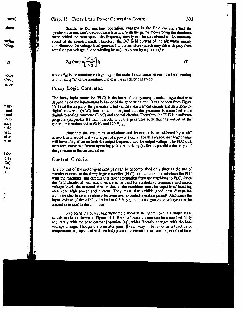
;ontrol
Xcinguling.
(’2)
?fore.
manyand
sand: out-%
rislicaltorein
d fixxltoDC
iture-3.
c*
! Chap. 15 Fuzzy Logic Power Generation Control 333
Similar to DC machine operation, changes in the field cumnt effect thesynchronous mtwhioe’s output characteristics. Withtheprimemoverbeingthedominantforce Mind the rotors- the frequatcy mostly can be contributed to the rotationalsped of the coupkd shaft- Therefore, the DC field current of the alternator mainlycontributesto the voltagelevel generatedin the armature(whichmaydiffexslightlyfromactual output voltage,due to windinglosses),as shownby equation(3}
(’3
whereEd is the armamrevoltage,~ is the mutual inductance belween the field winding
and winding “a” of the arrnatum, and w is the synchronoussped.
Fuzzy Logic Controller
The fuzzy logic controller (FIX) is the heart of the system; it makes logic deeisionsdependingon the input/output behavkr of the generatingunit. It can be seen fromFigure15-1 that the outputof the ge.nemmxis fed via the measurementcircuitsand an ana.bg-to-digital convemr (ADC) into the computer, and that the generator is controlled via adigital-to-analogconverter(DAC)and control circuits.Therefore,the FIX is a softwareprogram (Appendix B) that interacts with the generator such that the output of thegeneratoris maintainedat 60 Hzand 120Vm.S.
Note that the system is stand-alone and its output is not effected by a stiffnetworkas it wouldif it were a part of a power system.For this reason,any load changewill have a blg effea on both the output frequencyand the outputvoltage.‘he FIX will,therefore,moveto differentoperatingpoints, stabilizing(as fastas possibie)the outputofthe genemtcrto thede&redvalues.
Control Circuits
The conrrol of the motor-generatorpair can be accomplishcxlonly through the use ofcircuits externrdto the fuzzy logic unuroller(FK), i.e., circuitsM intetiacetheFLCwith the mzzhin~ and circuits that take informationfrom the machinesto FLC. Sincethe field circuits of both machinesare to be used for controlling frequencyand outputvoltage level, the external circuits tied to the machines must be capable of handlingrelatively high power and current. They must also exhibit good heat dissipationcharacteristksto avoidnonlinearbehavioroverextendedoperationperiods.Also,sincetheinput voltageof the ADC is limited to O-5V~, the output generator voltage must bealteredto be usedin themmputer.
Replacingthe bulky, inxcurate field rheostat in Figure 15-2 is a simple NPNtransistor circuit shown in Figure 154. Here, collector current can be controlled fairlyaccurately with the base current [equation(4)], which linearly changes with the basevoltage change. Though the transistor gain @) can vary in behavior as a functionoftemperature,a proper heat sink can help protect the circuit for reasonable periods of time. .
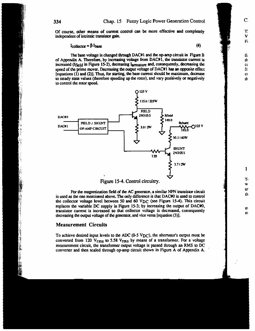
Iii,,
i!.’~
334 Chap. 15 Fuzzy Logic Power Generation Control
Of course, other means of currentcontrol can b rnofe effective md completelyindependentof intrinsictransistorgain.
buecta =B“baae (4)
‘l%ebase voltageis changedthmugbDAC#l snd the op-ampcircuit in FigureBof AppendixA l%erefore,by incmasingvoltage from DAC#l, the mmistor current isin- ~f~ld in F- 15-2),h=hlg ~a~ and, c~mdy. hing Ihespeedof the primemover.Decmsing theoutputvoltageof DAC#l b an oppositeeffect[equations(1) and (2)].Thus, for stardng,the basecunent shouldbe maximum,decmwto steadystate values (thereforespeedingup the rotor), and vary positivelyor negativelyto controlthe rotor speed.
#115.6IZ5W
Figure 15-4.Controlcircuitry. -
!j For the magnetizationf~ld of the ACgenerator,a similar NPN transistorcimit
fiis used as the one mentionedabove.Theonly differenceis that DAC#Ois used to controlthe collector voltage level between 50 and 60 VDC (see Figure 154). This circuit
~ replaces the variable DC supply in Figure 15-3; by increasing the output of DAC#O,
1“transistor current is increased so that collector voltage is decreased, consequently
,’ decreasing*output volrageof thegenerator,andviceversa [equadon(3)].
~!;,Measurement Circuits
11,~.II
i
To achieve desired input levels to the ADC(O-5VDC), the alternatm%output must be,,
1converted from 120 Vrms to 5.58 Vrms by means of a transformer. For a voltage
lkmeasurementcircuit, the transformeroutput voltage is passed through an RMS to DC
,+1 convetir and then scaled through op-ampcircuit shown in Figure A of Appndix A.
1c:
‘rv
~ ‘i
flhC(frC(th
1
T,w’arth
m
1m

(4)
igure Brremtis;ing thee effect
@ively
y v
Cilrwitcontrolcircuit‘AC#O,pently
lust be‘oltagetoDcdix A.
Chap. 15 Fuzzy Logic Power Generation Control 335
Therefore, the alternator voltage of 1- Vm~ is converted and to 0.172+.816VW in the input to the computer.A diagramof the measurementcircuitryis shown inFigure 15-5.
For the frequency measurementcircui~ the transformervoltageis nxtifkd andfd~daq-~kti ~~ofampmwititiaemthe ouqmt of the generator. This squarepulse is passed through a frquexwy to voltageconverter, and the output DC voltage of the converter is scaled with the opnp circuitfrom Figure A of Appendix A. Therefore,the alternatorfkquency betwexm5545 Hz isconverkxland scaled to 0.1724.816 VDC in the input to the computez.The diagramofthis circuit is also shown in Figure 15-5.
120 ACII
1
5.58 K
31N4001
LM339COhwwm
AD65auNwcoNV-ERlml
10M
u AD536AKDRMs/rx A:R&~ _QfY7
coNvImrER
Figure 15-5. Measurement circuitry.
15.3 FUZZY KNOWLEDGE BASE.
To be able to form a knowledge base the input and output signals had to be given aworkingrange.It wasdecidedthat the voltagecouldfluctuatein a mngebetween110Vmand 130Vms, and the frequencyin a rangebetweem55 Hz and 65 Hz.Thew rangeswemthen dividedinto sets, and eachset wasgivenmembetilp functions.
The next step was to form a knowledge base. But before that was possible,measurement of the inpuf/output behavior of the system was needed. From thesemeasurementsthe fiuzy rules werecreated.Hereis an exampleof makingof a fuzzyrule
– Changing load from infinityto 10WQ:
Flequency 60HZ + 57HZ - AF=3HZVoltage: 120VAC + 113VAC = AVAC= WAC
336 Chap. 15 Fuzzy Logic Power Generation Control
- CmtrOlactionsto get ~uewy back to 60Hzand voltage10120VAG
l~hunt: 0.310V~ + 0.261V~ - ~shunt = 4.049AKVf : 54.35V~ + %.8VX s AVf= 2.45VW
- Thenthefollowingtie is generatedfromthe fuzzyseW
IF APis LAND AVACis MTHEN Nahum is N AND AVfis P
whereL stands for the membership function Low, M for Medium, N forNegative,and P for Positive.
In this way, the entireset of rules weaeformed,basedon the changein inputand outpu~The final rule base is as follows. (Ah. L=Low, M=Medium, H=High, N=Negative,Z=zero, P=Positive)
Rule 1: IF AFis LAND AVACis LTHENAIshuntis N ANDAVfis N
Rule2: IF AFis LAND AVACis MTHENAIshuntis NAND AVfis Z
Rule3: IF AFis LAND AVACis HTHENAIshuntis N AND AVfis P
Rule4: IF AFis MANDAVACis LTHENAIshuntis Z AND AVfis N
Rule5: IF AFis MANDAVACis MTHENAIshuntis Z AND AVfis Z
.
Ruk%: lFAPis MANDAVACis HTHENAIshuntis Z AND AVfis P
Rule7: IF AFis HAND AVACis LTHENAIshuntis P AND AVfis N
Rule8: IF AFis HAND AVACis MTHENAIshuntis P AND AVfis Z
Rule9: IPAFis HAND AVACis HTHENAIshuntis P AND AVfis P
and the membershipfunctionsare shown in Pigures 15+, 15-7and 15-8.

~ontrol
Ac
,N for
output.:gative,
4 L M H1.o-
1Q 1.-
E I
1$ (
1s :
128 162 192 222 255
Frequency [counts]
Figure 15-6. Membership 1.0-
functions for input values of Q3controller. (a) Frequency (counts), ~ g
above; (b) Voltage (counts), right. ~ I5
0.o-
L M H
I
8
111I181
:I
128 162 192 222 255
Voltage [counts]
A N z P1.0-
1Q 1
I51n :~~ :g> ,
z :
-10 -6 0 6 10
AField voltage [counts]
Figure 15-7. Membership functionsfor output values of controller usingan 8-bit DAC. (a) Field voltage(above); (b) AShunt current (right).
N z P
1
1
1
I
1
1
111
I
I
10 -6 0 6 10
AShunt current [counts]
337

~!/i ‘1. 338 Chap. 15 Fuzzy Logic Power Generation Control
ii *N z P
1{ 0.0 ‘i / v \ 1 b-160136 -96 0 96
:. Afield voltageiII
(
‘i! Fimu-e 15-8. Membership finctionsl;’ foioutput values of controller using
,’~~
a 12-bit DAC. (a) AField voltage(above); (b) AShtmt cment (right).
1561“60
A N z P
1.0- .1 1
a. :I1
E20 :
It
2+ :11
g> , 1
z :11I
0.041 b
-160-136 -96 96 136160
AShunt current
lle fuzzy sets, their membership functions, and the fuzzy rules were thenassembled into a fuzzy knowledge base by using the Togai InfraLogic ~) Shell inMicrosoftWindows.l%e output file of the TIL Shell (AppendixC) was then compiledtogeneratea C-subroutine,whichwas then linked to the maincontrolprogmm.
‘,
15.4 EXPERIMENT
To test the system, a load unit was connected to the output of the generator. ‘his loadunit is a box of parallel comected resistors, and each resistor is activated by a switch.
il.. Figure 15-9showsthe load unit diagram.
I,!!~/:
+~\ \ \ \
Figure 15-9. Load unit.
:!‘1 Note thateaehadditionalloadckxs not add resistarteeon the outputbut decreasesI the resistanceand in that way demandspower. Thereforethe generator

K
Chap. 15 Fuzzy Logic Power Generation Control 339
power output, which requires more power to the DC-motor. Results in the followingsection were obtained by switching two load resistors at the same time in the followingsequmxz
1) NOLOAD2) R1-R2 ON3) R3-R4 ON4) R3-R4 OFF~ R1-R2 OFF
The loadswere turnedon/offat theme time @nts.
15.5 RESULTS
The frequency and voltage responses are shown in Figures 10 and 11, respectively. InFigure 15-10 (8-bit case), it can be seen that signals seule around their optimalvaluesbuttheir fluctuation is too big to be satisfactory. The problem is in the sensitivity of thecontrol signals, shown in Figures 12 and 13 (8-bit case); i.e., even though the systemoutputs are still not completely settled, the control signals have already settled becausechange in the input is too small to achieveany change in the output. Therefore,the 8-bitDAC has insufficient precision for this particular circfit.
q VRhbisca-bit): RwummZml ! 1 ! ! 1
I
160IJ
o 10 20 30 42 xl w 70
. l-ma [-1
Figure 15-10. Frequency response for 8- and 12-bit DAC.

Iii [Oat]
Figure 15-11. Voltage response for 8- and 12-bit DAC.
Time [SeG]
Figwe 15-12. Control signal froc~n~ond 12-bit DAC for field voltage.
340

60 70
60 m
)AC.
H...................
60 m
11......................................................................m m
field voltage
I
<’d
Chap. 15 Fuzzy Logic Power Generation Control341
‘Tine [60=1
~~t Vtile (lZ-bit) : ~~
Ual 1
-
3sm - .
!
‘*””’”””””””’-
-~*””””””””” /
‘3am -..: .,” .. . . . .. . .
‘rime [-1
Figure 15-13. Control signal from 8- and 12-bit DAC for shunt currentcontrol.
To solve this problem, the DAC bits are increased to 12, giving finer controlresolution. In Figures 10 and 11 (12-bit case), the results of the 12-bit controller areshown. As seen in Figure 15-10, the 12-bit case, the fluctuationsaround optimal valueswere significantly reduced, which supports the use of a more expensive DAC.Furthermore,the 12-bitDAC achievedsettlingof frequencyand voltagewith zero offset,as opposedto its 8-bit counterpart(seeFigures8 and 9).
Howevw, in Figure 15-10,them is an apparentineonsk~ncy in the second loaddisturbance.The 8-bit controller seems to suppressthe transientresponw better than the12-bit controller. This can be a misleading interpretationbecause the controller, at themoment of disturbance%was already executingrules to control steady state oscillations.Refernng to Figure 15-11,it can be seen that the controlvalueat that time is changinginthe oppositedirectionfromthat whichis neededto suppressthe new disturbance.Anotherreason for this ineonsis~ncy is the inherendy large time constanwin the system. Thesecharacteristicsachieverelativelyslowreqmnse times givensuddenchangesin the controlsignals. Therefore, in this case, these two system characteristicscaused this abnormallyl~ge overshotto occur.
342 Chap. 15 Fuzzy Logic Power Generation Control
15.5 CONCLUSION
In this chapter it is shown that fuzzy logic can be used with success in power systemscontrol. The main result, however, is that this method gives a simple way to design acontroller for a nonlinear system without complicated real-time modeling and expensivehardware. Future studies of rhis control scheme would be to develop a model of a powersystem, and compare this emrol method with other non-fuzzy control methods, as in [6].
REFERENCES
[1]
[2]
[31
[4]
[3
[Q
Hassan, M. A. M., Malik, O. P,, and Hope, G. S., A Fuzzy Logic BasedStabilizer for a Synchronous Machine, IEEE Tmns. on Energy Conversion,Sept. 1991, pp. 407413.
Hsu, Y.-Y., and Cheng, C.-H., Design of Fuzzy Power System Stabilisers forMulitmachine Power Systems, IEE Pmeedings-C, May 1990, Vol. 137, pp.233-238.
Hiyama, T., and Lim, C. M., Application of Fuzzy hgic Control Scheme forStability Enhancement of a Power System, IFAC Symposium on PowerSystems and Power Plant Control, Aug. 1989, Singapore.
David, A. K., and Rong&, Z., An Expert System with Fuzzy Sets for OptimalPlanning, IEEE Trans. on Power Systems, Feb. 1991, pp. 59-65.
Tomsovic, K, A Fuzzy Linear Programming Approach to the ReactivePowerlVoltage Control Problem, IEEETrans. on Power Systems, Feb. 1992,pp. 287-293.
Yousef, H., and Simaan, M. A., Model R~erence Aa@tive Control ofLargeScale Systems with Application to Power Systems, fEE Proceedings-D, July1991, Vol. 138, pp. 321-326.

eration Control
n power systemsway to design a
~gand expensivenodel of a powerelhods, as in [6].
gicBasedbnversion,
Stabilisers forvol. 137, pp.
rol Scheme form Power
etsfor Optimal;5.
eaclivens, Feb. 1992,
trol of Large4ngs-D, July
Chap. 15 Fuzzy Logic Power Generation Control
APPENDIX A
INPUT 5.01-6.12V O~m 0,172-4.816V
-15V
1
k
1
~ -5V10K
2
LM124
1 “14 33K
2 1 G3 x
4v+ v- -
11
5 2+
6 “2 - I lstm ‘:
7 8 10KI b o
x
343
I 10K I
Figwe A. A/D op-a.mp cimuit.
TO THE BASE OF 2N3055
DAC# 1LM124
10K 10K 1 14
210K DAC?#O
.
00 TO THE BASE RESISTOR
-15Vx OF 2N3055
o
120K
10K 3 -1 v
I100K
&2 lOOK
&
Figure B. Shunt/Field op-amp circuit.
“