2014 mayank baranwal.web.engr.illinois.edu/~salapaka/pdfs/pdfs/baranwal2014...application of field...

APPLICATION OF FIELD PROGRAMMABLE ANALOG ARRAYS (FPAAS) TOFAST SCANNING PROBE MICROSCOPY

BY

MAYANK BARANWAL

THESIS

Submitted in partial fulfillment of the requirementsfor the degree of Master of Science in Mechanical Engineering

in the Graduate College of theUniversity of Illinois at Urbana-Champaign, 2014

Urbana, Illinois

Adviser:

Professor Srinivasa Salapaka

Abstract

For a long time, signal processing used to be accomplished by microprocessors and DSPs (Digital Signal

Processors). The advent of reconfigurable computing devices, such as Complex Programmable Logic Devices

(CPLDs) and Field Programmable Gate Arrays (FPGAs) has given a new dimension to signal processing

applications [1] by not only allowing users to customize the hardware to suit the specific requirements but

also making high speed applications a possibility, too. More recently, Field Programmable Analog Arrays

(FPAAs) have emerged as interesting alternatives to most signal processing based applications [2]. Even

though the use of FPAA devices is still limited due to small number of suppliers, a growing interest in

using FPAAs for various engineering applications is expected [3]. In this thesis, we exploit the FPAAs to

demonstrate their usefulness and ease of implementation in developing fast and robust controllers for an

Atomic Force Microscope (AFM) unit.

Atomic Force Microscopes (AFMs) are getting faster. However, video-rate imaging still remains a big

challenge to the AFM community [4]. Therefore AFMs are required to have very fast nanopositioning sys-

tems. However, high-bandwidth requirement on the positioning system poses fundamental limitations on

the image resolution [5]. The resolution of an image depends on the controller’s capabilities to attenuate

the measurement noises. Tools from robust control theory [6], [7] are employed to not only quantify the

measurement noises and parametric uncertainties, but also synthesize the controllers in an optimal setting.

However, implementation of such controllers require electronics that can support high-bandwidth op-

erations. Field Programmable Analog Arrays (FPAAs) [8], which have bandwidth up to 400 kHz, have

been employed to demonstrate not only the direct implementation of these controllers in terms of transfer

functions, but also high-bandwidth tracking performance, too, when compared to most other commer-

cially available Digital Signal Processors (DSPs). A significant improvement in the closed-loop bandwidth

(∼ 500Hz) has been demonstrated. A part of the work is dedicated to the Q-control of microcantilevers [9].

Since, cantilevers are second-order flexible structures with high resonant frequencies (∼ 50kHz) , Q-control

of cantilevers requires estimating velocity at resonant frequencies. High-bandwidth advantage of FPAAs can

be exploited to achieve the desired Q-control.

ii

To my grandfather and my mother, for their endless love and support

iii

Acknowledgments

First, I would like to sincerely thank my adviser Prof. Srinivasa Salapaka for his patience and guidance.

Apart from the knowledge he’s been imparting in me through various useful discussions on varied topics

ranging all the way from research to the current state of politics, I always admire his humility and positive

attitude towards the students. Also, a heartfelt thanks to him for taking care of me when I was going

through a stressful phase.

I would also like to express my gratitude to my research colleagues Gayathri, Mashrafi, Yunwen and in

particular, Ram for not only being a good friend and helping me out on the research front, but also for

taking time out to show my parents around when they were in town.

Graduate life in Urbana-Champaign has been a fun-filled journey and I owe this to my friends Piyush,

Pranav, Prakalp, Shishir and Srikant.

All through my stay at UIUC, my family has always supported me through their love and encouragement.

It’s only fair to thank Almighty for having given me a wonderful family to whom I could always look up to

for advice and encouragement.

Last, I would like to extend my deepest regards to some of the greatest teachers and researchers at UIUC

for instilling confidence and motivation in me to keep striving for excellence.

iv

Table of Contents

List of Tables . . . . . . . . . . . . . . . . . . . . . . . . . . . . . . . . . . . . . . . . . . . . . . vi

List of Figures . . . . . . . . . . . . . . . . . . . . . . . . . . . . . . . . . . . . . . . . . . . . . . vii

List of Abbreviations . . . . . . . . . . . . . . . . . . . . . . . . . . . . . . . . . . . . . . . . . viii

List of Symbols . . . . . . . . . . . . . . . . . . . . . . . . . . . . . . . . . . . . . . . . . . . . . ix

Chapter 1 Introduction . . . . . . . . . . . . . . . . . . . . . . . . . . . . . . . . . . . . . . . 1

Chapter 2 System Description . . . . . . . . . . . . . . . . . . . . . . . . . . . . . . . . . . . 42.1 Hardware Description . . . . . . . . . . . . . . . . . . . . . . . . . . . . . . . . . . . . . . . . 4

2.1.1 Anadigm FPAA . . . . . . . . . . . . . . . . . . . . . . . . . . . . . . . . . . . . . . . 42.1.2 X-Y Nanopositioning System . . . . . . . . . . . . . . . . . . . . . . . . . . . . . . . . 62.1.3 NI-DAQmx PCIe-6361 . . . . . . . . . . . . . . . . . . . . . . . . . . . . . . . . . . . . 6

2.2 System Identification . . . . . . . . . . . . . . . . . . . . . . . . . . . . . . . . . . . . . . . . . 72.2.1 NI-LabView Swept-Sine Measurement VI . . . . . . . . . . . . . . . . . . . . . . . . . 72.2.2 Piezo stage system identification . . . . . . . . . . . . . . . . . . . . . . . . . . . . . . 82.2.3 Cantilever system identification . . . . . . . . . . . . . . . . . . . . . . . . . . . . . . . 11

Chapter 3 Control Design Algorithms for the Nanopositioning System . . . . . . . . . . 153.1 Feedback only control design . . . . . . . . . . . . . . . . . . . . . . . . . . . . . . . . . . . . 153.2 2-DOF H∞ control . . . . . . . . . . . . . . . . . . . . . . . . . . . . . . . . . . . . . . . . . . 183.3 2DOF Model-Matching control . . . . . . . . . . . . . . . . . . . . . . . . . . . . . . . . . . . 193.4 2DOF Optimal Robust Model Matching Control . . . . . . . . . . . . . . . . . . . . . . . . . 21

Chapter 4 Controller Implementation on FPAA and Experimental Results . . . . . . . . 234.1 Balanced Realization and Model Reduction . . . . . . . . . . . . . . . . . . . . . . . . . . . . 234.2 1DOF H∞ control design . . . . . . . . . . . . . . . . . . . . . . . . . . . . . . . . . . . . . . 244.3 2DOF H∞ control design . . . . . . . . . . . . . . . . . . . . . . . . . . . . . . . . . . . . . . 274.4 2DOF Model-Matching control . . . . . . . . . . . . . . . . . . . . . . . . . . . . . . . . . . . 304.5 2DOF Optimal Robust Model Matching control . . . . . . . . . . . . . . . . . . . . . . . . . . 31

4.5.1 Reduced-order controller for Y-stage . . . . . . . . . . . . . . . . . . . . . . . . . . . . 324.5.2 High-order controller for X-stage . . . . . . . . . . . . . . . . . . . . . . . . . . . . . . 32

Chapter 5 Q-Control of Microcantilevers . . . . . . . . . . . . . . . . . . . . . . . . . . . . 385.1 Introduction . . . . . . . . . . . . . . . . . . . . . . . . . . . . . . . . . . . . . . . . . . . . . . 385.2 Velocity estimation using modulation-demodulation approach . . . . . . . . . . . . . . . . . . 395.3 Q-control implementation on FPAA and Experimental results . . . . . . . . . . . . . . . . . . 42

Chapter 6 Conclusion and Future Work . . . . . . . . . . . . . . . . . . . . . . . . . . . . . 44

References . . . . . . . . . . . . . . . . . . . . . . . . . . . . . . . . . . . . . . . . . . . . . . . . 45

v

List of Tables

2.1 Qualitative comparison of reconfigurable technologies . . . . . . . . . . . . . . . . . . . . . . . 5

vi

List of Figures

2.1 Control system set-up for the flexure stage . . . . . . . . . . . . . . . . . . . . . . . . . . . . . 52.2 A custom designed PCB for interfacing FPAA with the AFM . . . . . . . . . . . . . . . . . . 62.3 Piezo driven flexure 2DOF scanner in an AFM . . . . . . . . . . . . . . . . . . . . . . . . . . 72.4 NI PCIe-6361 . . . . . . . . . . . . . . . . . . . . . . . . . . . . . . . . . . . . . . . . . . . . . 82.5 System identification for the X-stage using Swept-Sine Measurement VI . . . . . . . . . . . . 92.6 Frequency response results for the piezo-stages . . . . . . . . . . . . . . . . . . . . . . . . . . 102.7 Schematic of AFM showing all the fundamental components. In the pictured configuration,

both vertical and lateral piezos are located in the base or scanning stage. . . . . . . . . . . . 122.8 Frequency response results for the cantilever subsystem . . . . . . . . . . . . . . . . . . . . . 14

3.1 Schematic of feedback only control design . . . . . . . . . . . . . . . . . . . . . . . . . . . . . 163.2 Generalized plant for 1DOF H∞-control design . . . . . . . . . . . . . . . . . . . . . . . . . . 163.3 A 2DOF control architecture . . . . . . . . . . . . . . . . . . . . . . . . . . . . . . . . . . . . 183.4 Generalized plant for 2DOF H∞ control . . . . . . . . . . . . . . . . . . . . . . . . . . . . . . 183.5 Model matching through the prefilter problem . . . . . . . . . . . . . . . . . . . . . . . . . . . 193.6 A 2DOF optimal robust model matching control design . . . . . . . . . . . . . . . . . . . . . 223.7 Generalized plant for optimal 2DOF robust model matching controller . . . . . . . . . . . . . 22

4.1 Experimental setup for controlling the nanopositioning system . . . . . . . . . . . . . . . . . 244.2 Theoretical S and T for 1DOF H∞ control . . . . . . . . . . . . . . . . . . . . . . . . . . . . 254.3 Designing reduced order feedback controller on an FPAA using AnadigmDesiner2 software . . 254.4 Tracking performance using a 1DOF H∞-control design . . . . . . . . . . . . . . . . . . . . . 264.5 Choice of Wr and Wn weighting functions . . . . . . . . . . . . . . . . . . . . . . . . . . . . . 274.6 S and T for mixed-sensitivty 2DOF H∞ control . . . . . . . . . . . . . . . . . . . . . . . . . . 284.7 Tracking performance using a 2DOF H∞-control design . . . . . . . . . . . . . . . . . . . . . 294.8 S and T for model-matching control . . . . . . . . . . . . . . . . . . . . . . . . . . . . . . . . 304.9 Tracking performance using a 2DOF optimal prefilter based design . . . . . . . . . . . . . . . 314.10 S and T for model-matching control . . . . . . . . . . . . . . . . . . . . . . . . . . . . . . . . 324.11 S and T for optimal robust 2DOF H∞ loop-shaping controller for the Y-stage . . . . . . . . . 334.12 Tracking performance using a 2DOF optimal robust H∞ loopshaping control for the Y-stage 344.13 Daisy chaining two FPAAs to implement higher-order controller . . . . . . . . . . . . . . . . 354.14 Tracking performance using a 2DOF optimal robust H∞ loopshaping control for the X-stage 364.15 S and T for optimal robust 2DOF H∞ loop-shaping controller for the X-stage . . . . . . . . . 37

5.1 Schematic for velocity estimation . . . . . . . . . . . . . . . . . . . . . . . . . . . . . . . . . . 405.2 Implementing Modulation-Demodulation on FPAA . . . . . . . . . . . . . . . . . . . . . . . . 415.3 Schematic of Q-factor control of a microcantilever . . . . . . . . . . . . . . . . . . . . . . . . 425.4 Estimating velocity using modulation-demodulation approach . . . . . . . . . . . . . . . . . . 43

vii

List of Abbreviations

AFM Atomic Force Microscope

CPLD Complex Programmable Logic Device

DOF Degree Of Freedom

DSP Digital Signal Processor

DTFT Discrete-Time Fourier Transform

FPAA Field Programmable Analog Array

FPGA Field Programmable Gate Array

NI National Instruments

PID Proportional Integral Derivative

PSD Power Spectral Density

SPM Scanning Probe Microscope

TITO Two-Input-Two-Output

viii

List of Symbols

Symbol Description

G(s) Plant transfer function

P (s) Generalized Plant transfer function

Gxx(s) X-stage transfer function

Gyy(s) Y-stage transfer function

Gzz(s) Z-stage transfer function

Gdd(s) Dither to Deflection transfer function

Gzd(s) Z-piezo to Deflection transfer function

Kfb(s) Feedback controller transfer function

Kff (s) Feedforward controller transfer function

Kpre(s) Prefilter transfer function

S(s) Sensitivity transfer function

T (s) Complementary Sensitivity transfer function

e Tracking error

n Measurement error

d External disturbance

ix

Symbol Description

u Control input

r Reference input

w Exogenous input

z Regulated output

v Regulated output

y Sensor output

Ws(s) Sensitivity weighting transfer function

Wt(s) Complementary Sensitivity weighting transfer function

Wu(s) Control weighting transfer function

Tref (s) Reference transfer function

AM −AFM Amplitude Modulation AFM

Q Quality factor

ωn Natural frequency

x

Chapter 1

Introduction

Having described the advantages with an FPAA device, the aim of this thesis is to highlight two main compo-

nents: (a) Control design to improve the bandwidth and tracking performance of a 2-DOF nanopositioning

system used in Atomic Force Microscopes (AFMs), and (b) Control implementation on a Field Programmable

Analog Array (FPAA). We use tools from robust control theory to design and implement 2DOF controllers

for the nanopositioning system. The implementation of higher-order model-based controllers on FPAAs has

results in significant improvement in tracking bandwidths when compared to implementing similar control

algorithms on a DSP hardware as in [5, 10], mainly due to the low sampling rate constraints and limited

number of resources. Moreover, more complex functions such as multiplying signals and generating sinu-

soidal signals to achieve Q-control of high resonant frequency (∼50kHz) cantilevers has been successfully

achieved using high-bandwidth advantage of FPAAs.

A typical nanopositioning system used in a Scanning Probe Microscope (SPM) is comprised of a flexure

stage, and actuators (typically piezoelectric) and/or sensors along with the feedback system. A systems

viewpoint of the nanopositioning system is presented. The main goals of the control design are to achieve

high position tracking bandwidth, resolution, and robustness to modeling and environmental uncertainties.

The framework used to analyze and control the precision systems is quite general and can be easily extended

to other systems as in [11].

It has been a common practice to design Proportional Integral Derivative (PID) controllers for such

systems as they are easily implementable. However, the PID controller design does not offer flexibility in

design, robust stability property, high bandwidth and high resolution. Also, PID controllers require the

gains to be manually tuned without offering much insight into robustness.

This work exploits the control design tools developed for positioning systems in SPM earlier [12]. However,

the controllers have been implemented on an FPAA [8]. FPAA offers not only design and implementation of

very high bandwidth controllers (∼400kHz), but their direct realization in terms of transfer functions. 1DOF

H∞ control of positioning system using FPAA has been demonstrated earlier in [13]. However, the aim of

this thesis is to highlight the significance of 2DOF control over 1DOF control and simultaneously implement

1

higher order 2DOF controllers using FPAA. For instance, Glover-McFarlane control design [5, 14] has resulted

in better repeatability of tracking performance of the nanopositioning systems than feedback only control.

In Glover-McFarlane control design, an add-on controller block is wrapped around an existing controller,

thereby making the nanopositioning system insensitive to external disturbances, modeling uncertainties

and sensor noise. Similarly, a 2DOF H∞ control design with both feedforward and feedback controllers

shows significant improvement over the feedback only design as in the 2DOF setup, the reference signal gets

prefiltered before being fed to the original plant, thereby providing an additional degree to the system.

In SPMs, microcantilevers are used to extract sample topographical information. Q-factor of a micro-

cantilever is the measure of its sensitivity. Equivalently, Q-factor characterizes the bandwidth of a cantilever

around the center (resonant) frequency. Cantilever dynamics play an important role in Tapping mode

AFM (AM-AFM) [15]. Higher Q-factor corresponds to high-sensitivity of cantilevers and low tip-sample

interaction force and is more suitable for biological samples, whereas, low Q-factor allows faster scans with

limited resolution. A normal microcantilever has resonant frequency in the orders of few hundreds of kHz.

High-bandwidth advantage with FPAAs can be exploited to achieve the desired Q-control.

This thesis shows the design and implementation of four different control algorithms namely the 1DOF

H∞ design, 2DOF H∞ design, Model-matching control design and Glover-McFarlane control design for the

X-Y positioning stages in an AFM. In addition, the control hardware is the Anadigm Field Programmable

Analog Array (FPAA) hardware combined with MFP-3D AFM. The 2DOF control designs when imple-

mented on the AFM have given substantial improvements in bandwidth (as high as 480Hz) for the same

resolution and robustness. Other performance objectives can be improved by appropriately designing the

weight function or target transfer function. This thesis also shows how to estimate cantilever tip-velocity for

achieving desired Q-control. Cantilevers are flexible structures with relatively sharper resonant frequencies.

Hence, the velocity signal is orthogonal to the deflection signal with the same resonant frequency. Orthogonal

signal of a given ∼50kHz signal has been experimentally demonstrated in this work.

Improvements in the tracking performance of the nanopositioning system and the corresponding Q-factor

control of the microcantilever would mean faster scan rate and hence, video-rate imaging. Novel research

and study of biological processes would then be possible with this added capability of the AFM hardware.

A low-resolution video imaging of walking Myosin has been reported in [4]. With the advantage of robust

control theory to be able to quantify the resolution and bandwidth, fast controllers with specified resolution

can be easily designed and implemented.

The organization of this thesis is as follows. Chapter 2 describes the system details of the AFM and

the FPAA hardware, system identification of the positioning system and other subsystems, model fitting

2

and model reduction. Chapter 3 describes the design of various controllers - 1DOF H∞, 2DOF H∞, Model-

matching and Glover-McFarlane controllers. Chapter 4 showcases implementation of aforementioned con-

trollers onto FPAA hardware and discusses the experimental and simulation results. Chapter 5 discusses the

setup for Q-control of microcantilevers and discusses the experimental results. This is followed by discussion

on further extension of this work.

3

Chapter 2

System Description

2.1 Hardware Description

2.1.1 Anadigm FPAA

Reconfigurable computing (FPAAs and FPGAs) has provided solutions to countless engineering problems.

For most signal processing applications, FPAAs are clearly the most suited alternatives when compared

to their digital counterparts - FPGAs. With the use of floating-gate devices in the core element in the

programmable signal processing FPAA [16], this technology offers integration of a larger number of elements

per chip, high precision and high efficiency gain when compared to DSP processors.

A brief comparison of the FPAA and the FPGA technologies has been presented in [17]. Regarding the

expressiveness of the transfer function models in the reconfigurable devices, the FPAA approach, because of

its analog implementation, is closer to mathematical models than the FPGA approach, which doesn’t exactly

portray the exact mathematical model because of the Z-transform and quantization. Moreover, FPGAs

demand sound understanding of system resources and allocation, etc. In contrast, filter-design in FPAAs

thrives on simple op-amps based circuit that can be easily configured using the provided development tools

and software. Moreover, FPAA devices are cheaper than their digital counterparts. Moreover, the FPAAs

supplied by Anadigm [8] has the advantage of having multiple functional blocks ready to use and, therefore,

the analog implementation is straightforward.

Although, a direct comparison is not possible, current FPGA devices seem to have larger device capacity

than the FPAA devices. However, two FPAAs can be used in series to implement up to a sixteenth-order

analog filter. The maximum operation frequency of the devices may limit their use in some applications.

The Anadigm FPAA used in this thesis runs at 16 MHz and can process signals up to 2 MHz. FPGAs, on

the other hand can operate at much higher frequencies (500 MHz). However, this is severely constrained by

the optimization and implementation done by the design software. All the above aspects of FPAA devices

make them preferred choice for control systems application. In the context of the desired control systems

4

Table 2.1: Qualitative comparison of reconfigurable technologies

Design Parameter FPAA FPGAEase of Implementation for control systems application +++ -Design Tools and Software +++ ++Cost +++ +Performance +++ +++Capacity + ++Running Frequency + +++Gain + ++Power Consumption - +

+++ excellent ++ good + average - weak

application to an AFM, this comparison cab be summarized as:

The control design is implemented on an Anadigm FPAA [18] using AnadigmDesigner2 EDA software.

Field programmable analog arrays (FPAAs) from Anadigm give an analog equivalent to the FPGA, thereby

allowing design of complex analog signal processing functions into an integrated, drift-free, pre-tested device.

The set-up of the control system is shown in Fig. 2.1.

Figure 2.1: Control system set-up for the flexure stage

FPAA [8] offers direct realization of very high bandwidth controllers (∼ 400kHZ) by employing Anadig-

mDesigner2 EDA software. The software allows designer to construct complex analog functions using con-

figurable analog modules (CAMs) as building blocks. With easy-to-use drag-and-drop interface, the design

process can be measured in minutes allowing complete analog systems to be built rapidly, simulated immedi-

ately, and then downloaded to the FPAA chip for testing and validation. A custom designed PCB (see Fig.

2.2) is used to interface single-ended 10V AFM signals with 0− 3.3V differential signals referenced at 1.5V.

This is achieved by using operational amplifiers AD-8130 and AD-8132 (Analog Devices, Norwood, MA,

USA) to scale and convert differential signals to single-ended signals and vice versa. Even though FPAA

offers very high flexibility in terms of designing and implementing high-order, high-bandwidth controllers; it

is relatively more sensitive to electrical noises when compared to its digital counterpart - FPGA. Also, the

5

Figure 2.2: A custom designed PCB for interfacing FPAA with the AFM

CAMs can’t be configured very accurately to model an exact given transfer function. This may result in a

slightly different control design than expected. However, this effect is usually very small and can be ignored

in most cases.

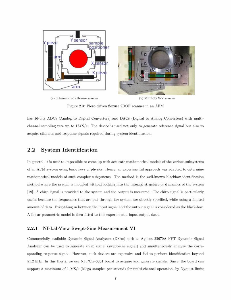
2.1.2 X-Y Nanopositioning System

A schematic of the X-Y nanopositioning system (MFP-3D X-Y scanner) is shown in FIg. 2.3. The scanner

has two flexure components with component ‘X’ stacked over the ‘Y’ where the sample holder is carried by the

X-component. Both stages can deform under the application of force, thereby providing the required motion.

These forces are generated using stacked-piezos. There are three piezoactuators in series for each axis. The

motion of each flexure component is measured by the corresponding nanopositioning sensors which are

modified from the linear variable differential transformer (LVDT) and the associated demodulation circuit.

The piezoactuators lead to a travel range of 90µm in a closed loop in both directions. The nanopositioning

sensors have noise less than 0.6nm (deviation) over 0.1− 1kHz bandwidth.

2.1.3 NI-DAQmx PCIe-6361

NI PCIe-6361 (Fig. 2.4) is an X series multifunction data acquisition (DAQ) device with high-throughput

PCI Express bus, NI-STC3 timing synchronization technology, and multicore-optimized driver. The device

6

(a) Schematic of a flexure scanner (b) MFP-3D X-Y scanner

Figure 2.3: Piezo driven flexure 2DOF scanner in an AFM

has 16-bits ADCs (Analog to Digital Converters) and DACs (Digital to Analog Converters) with multi-

channel sampling rate up to 1MS/s. The device is used not only to generate reference signal but also to

acquire stimulus and response signals required during system identification.

2.2 System Identification

In general, it is near to impossible to come up with accurate mathematical models of the various subsystems

of an AFM system using basic laws of physics. Hence, an experimental approach was adapted to determine

mathematical models of such complex subsystems. The method is the well-known blackbox identification

method where the system is modeled without looking into the internal structure or dynamics of the system

[19]. A chirp signal is provided to the system and the output is measured. The chirp signal is particularly

useful because the frequencies that are put through the system are directly specified, while using a limited

amount of data. Everything in between the input signal and the output signal is considered as the black-box.

A linear parametric model is then fitted to this experimental input-output data.

2.2.1 NI-LabView Swept-Sine Measurement VI

Commercially available Dynamic Signal Analyzers (DSAs) such as Agilent 35670A FFT Dynamic Signal

Analyzer can be used to generate chirp signal (swept-sine signal) and simultaneously analyze the corre-

sponding response signal. However, such devices are expensive and fail to perform identification beyond

51.2 kHz. In this thesis, we use NI PCIe-6361 board to acquire and generate signals. Since, the board can

support a maximum of 1 MS/s (Mega samples per second) for multi-channel operation, by Nyquist limit;

7

Figure 2.4: NI PCIe-6361

the identification can be performed up to a theoretical maximum of 500 kHz. This is a significantly better

than commercially available DSAs.

We use the ‘NI Swept-Sine Measurement’ example to measure the frequency response and harmonic

distortion of a device under test (DUT). Identification up to 300 kHz has been experimentally demonstrated

in this thesis. Fig. 2.5 shows frequency response measurements for the nanopositioning system using NI

PCIe-6361 and Swept-Sine Measurement VI.

2.2.2 Piezo stage system identification

The chirp-signal based system identification yields following results for the the three stages - X, Y and Z

(see Fig. 2.6): Clearly, the positioning piezos’ bandwidth is approximately 1 kHz. We are anyway not

interested in the dynamics beyond this frequency regime. MATLAB invreqs command is used to fit a linear

parametric model through the frequency response data. Weighted iterative least square fitting was performed

8

Figure 2.5: System identification for the X-stage using Swept-Sine Measurement VI

9

(a) X-stage frequency response

(b) Y-stage frequency response

Figure 2.6: Frequency response results for the piezo-stages

10

(c) Z-stage frequency response

Figure 2.6: (cont.) Frequency response results for the piezo-stages

over 0-2kHz and the reduction through balanced realization [6] resulted in the following parametric models:

Gxx =−0.022119(s+ 2.954× 104)(s+ 8117)(s− 8151)(s+ 418.9)(s2 + 890.2s+ 1.131× 107)

(s+ 1796)(s+ 217.1)(s2 + 717.5s+ 1.013× 107)(s2 + 1827s+ 3.751× 107)

× (s2 + 1185s+ 4.616× 107)(s2 + 350.3s+ 1.175× 108)(s2 + 452.4s+ 1.494× 108)

(s2 + 1440s+ 7.142× 107)(s2 + 267.1s+ 1.182× 108)(s2 + 605.8s+ 1.473× 108)(2.2.1)

Gyy =0.025231(s+ 1329)(s2 + 1008s+ 1.673× 107)

(s+ 738.8)(s2 + 981.1s+ 3.574× 106)

× (s2 + 508s+ 5.426× 107)(s2 − 1.172× 104s+ 1.097× 108)

(s2 + 1213s+ 2.35× 107)(s2 + 483.8s+ 6.512× 107)(2.2.2)

Gzz =−0.17329(s− 2.174× 104)(s2 + 241.8s+ 4.317× 107)(s2 + 855.5s+ 1.001× 108)

(s+ 1.347× 104)(s2 + 125s+ 4.333× 107)(s2 + 640s+ 9.771× 107)

× (s2 + 709.8s+ 2.279× 108)(s2 + 3864s+ 5.538× 108)

(s2 + 1140s+ 1.933× 108)(s2 + 717.7s+ 2.338× 108)(2.2.3)

2.2.3 Cantilever system identification

A schematic of the components fundamental to AFM operation is shown in Fig. 2.7. The “brain” of the

AFM is located in the AFM head. A cantilever with an extremely sharp tip is mounted at the bottom of the

head. Every variation of the surface height varies the force acting on the tip and therefore varies the bending

of the cantilever. This bending is measured by a sensing mechanism located in the AFM head. The sensing

mechanism comprises of a laser beam incident on the cantilever and reflected onto a split photo-sensitive

11

diode (PSD). Deflection of the cantilever owing to tip-sample interactions results in change of laser incidence

angle, which is captured by change in location of the laser spot on the PSD. The base of the cantilever is

Figure 2.7: Schematic of AFM showing all the fundamental components. In the pictured configuration, bothvertical and lateral piezos are located in the base or scanning stage.

attached to a dither piezo also called as the shake piezo. During dynamic scans, the dither piezo is used to

oscillate the cantilever sinusoidally. This piezo typically has very high bandwidths in the order of 600 kHz to

accommodate similar orders of cantilever resonance frequencies. Also, the Z-piezo actuator is located along

with the cantilever and the laser optic arrangement, in the AFM head. As a result, the Z-piezo actuation

causes vertical movement of the cantilever along with its base. Typical travel for the z piezo is around 15µm.

The type of setup for the AFM allows the movement of cantilever tip through not only dither piezo

but Z-piezo too. Typical dynamic imaging modes rely only on the dither piezo to produce a set-amplitude

sinusoidal actuation of the cantilever tip and measure the change in amplitude to accordingly vertically

actuate the cantilever arrangement using Z-piezo. This mode of imaging typically requires several cycles

to measure the amplitude change and is a hindrance to video-rate imaging. A new form of dynamic mode

imaging has been proposed in [20], that uses the Z-piezo as a low bandwidth controller and the dither piezo

as a high bandwidth controller for controlling the cantilever deflection, thereby eliminating the need to wait

for several cycles to measure the amplitude change.

Hence, the cantilever subsystem is viewed as a TITO (Two-Input-Two-Output) system in which the

low-voltage signals to the dither and Z piezos are the inputs and the cantilever ‘Deflection’ and ‘Z sensor’

are the outputs. This results in four input-output transfer functions Gdd, Gzd, Gzz and Gdz. By virtue of the

AFM head design; there is hardly any change in the Z-sensor measurements by actuating the dither piezo.

Therefore, Gdz ≈ 0 for all practical purposes. Also, Gzz is independent of the choice of cantilever and has

12

been identified in the previous section. The identification was performed for two different cantilevers - low

frequency (1st mode: ∼12.6 kHz, 2nd mode: ∼76.3 kHz); and high frequency (1st mode: ∼270 kHz). Fig.

2.8 shows the experimental frequency response results for the two cantilevers.

It can be seen that for the high resonant frequency cantilever, Gzd ≈ 0 with a very small but observable

peak at the resonant frequency 270 kHz. The reason being that the Z-piezo has limited bandwidth (¡ 10kHZ)

and dither-to-deflection amplification for this cantilever is almost non-existent in the low frequency regime.

The deflection signal has significant amplification only near the resonant frequency at 270 kHz, thereby

making deflection signal insensitive to Z-piezo actuation. This also limits the choice of cantilevers that can

be used to image samples using the approach described in [20].

13

(a) Frequency response data for low-frequency cantilever

(b) Frequency response data for high-frequency cantilever

Figure 2.8: Frequency response results for the cantilever subsystem

14

Chapter 3

Control Design Algorithms for theNanopositioning System

The nanopositioning system comes with a tunable PI only controller with a maximum scan rate of 1 Hz.

The most common approach to increasing tracking bandwidth is to increase the resonance frequency of a

nanopositioning system by building devices that are sufficiently stiff and small. However, building small

scanning devices limits the maximum traversal of the system to a few microns. The work in this thesis is

focused on designing and implementing high-end controllers giving robust stability, high bandwidth, high

resolution, disturbance rejection and noise attenuation without changing the basic design of the flexure stage.

There have been several approaches to improve the resolution and accuracy of the positioning system.

These include - feedforward implementation [21, 22]; using charge amplifiers instead of voltage amplifiers

to reduce hysteresis [23]; and feedback control designs with large gains at low frequencies [24, 25]. The

feedback control framework presented in [25] uses the tools from robust control theory to determine and

quantify the trade-offs between performance objectives and assess if it’s feasible to design a controller, given

the desired specifications. Most recently, 2DOF control design framework [26, 27, 28] is being employed

where the regular feedback control is appended with a feedforward scheme for the reference signal. 2DOF

control design which deals with the reference and the measured output signal separately has better capability

to satisfy robustness and performance objectives.

This thesis presents control design for the Y-stage using - 1) 1DOF H∞ framework, 2) 1DOF H∞

framework, 3) 2DOF Model-Matching framework and 4) 2DOF Glover-McFarlane robustifying framework.

The shortcomings of the 1DOF control design can be seen to be successfully eliminated in the 2DOF setup.

The details of the various control designs are as follows:

3.1 Feedback only control design

Fig. 3.1 shows the schematic of a 1DOF (Feedback only) control design.

Instead of designing a tunable PI/PID filter for the feedback control, which doesn’t offer much insights

into the closed-loop system stability and robustness issues, a 1DOF H∞ control framework is presented. The

15

Figure 3.1: Schematic of feedback only control design

performance and robustness objectives can be directly specified by specifying requirements on the ‘sensitivity’

and the ‘complementary sensitivity’ transfer functions. Fig. 3.2 shows a generalized plant for 1DOF H∞

control design framework.

Figure 3.2: Generalized plant for 1DOF H∞-control design

From Fig. 3.2,

e = r − y − n = r −G.u− n = r −GKe− n (3.1.1)

e = (1 +GK)−1(r − n) = S(r − n) (3.1.2)

y = GKe = GK.(1 +GK)−1(r − n) = T (r − n) (3.1.3)

u = Ke = KS(r − n) (3.1.4)

S = 1/(1 +GK) (3.1.5)

T = GK/(1 +GK) (3.1.6)

S + T = 1 (3.1.7)

16

where, S is the sensitivity transfer function, which is a closed-loop transfer function from reference r to

tracking error e, and T , known as the complementary sensitivity transfer function, is the closed-loop transfer

function from reference r to the system output y. S can also be represented as dy/ydG/G that represents the

percentage change in the plant model. Therefore, S is a measure of robustness of the closed-loop system to

modeling and parametric plant uncertainties. A general rule of thumb is to not allow the sensitivity transfer

function to have peak value beyond 6 dB, i.e.,

||S||∞ < 2 (3.1.8)

The bandwidth ωB is determined based on the frequency corresponding to the point where Bode plot of

the sensitivity transfer function crosses the -3 dB line from below. For larger bandwidth, it is required that

S crosses -3 dB line as later as possible. However, because of the algebraic constraint, S+T = 1, increasing

ωB would mean that T would still be large for relatively higher frequencies. Because, T also represents

the closed-loop transfer function from noise n to output y, this would result in significant amplification of

high-frequency noise, thereby resulting in poor tracking performance. Similar to ωB , ωBT is the bandwidth

based on the complementary sensitivity transfer function T , defined by its crossing of the -3 dB line from

above. For better resolution, i.e., better noise mitigation, ωBT should be small.

Similarly, KS is the closed-loop transfer function from tracking error e to controller output u. KS needs

to be bounded so that the controller output u is bounded. Since, in case of MFP-3D, the maximum absolute

voltage the piezo-actuators can safely handle is ∼ 10V, bounding controller output to avoid controller

saturation and device failure is important.

All these design constraints on the various closed-loop transfer functions are specified using inverse

weighing functions Ws, Wu and Wt. The optimization problem then is to solve for all stabilizing controllers

K posed in the stacked sensitivity framework,

minK∈K

∥∥∥∥∥∥∥∥∥∥WsS

WuKS

WtT

∥∥∥∥∥∥∥∥∥∥∞

(3.1.9)

where, K is a set of all stabilizing controllers.

17

3.2 2-DOF H∞ control

Because of the various algebraic and design constraints, the feedback only scheme has certain performance

limitations, which can be alleviated by using a 2DOF architecture shown in Fig. 3.3.

Figure 3.3: A 2DOF control architecture

In contrast to the feedback-only scheme described in previous section,where the controller acts only on

the difference between the reference r and the position-measurement ym, in the 2DOF scheme, the controller

acts independently on them. The generalized plant for a 2DOF H∞ control framework is shown in Fig. 3.4.

From the Fig. 3.4,

Figure 3.4: Generalized plant for 2DOF H∞ control

18

Tracking error, e = Serr + Tn (3.2.1)

Position, y = Tyrr − Tn (3.2.2)

Control (actuation) signal, u = S(Kff +Kfb)r − SKfbn (3.2.3)

S + T = 1 (3.2.4)

Ser = S(1−GKff ) (3.2.5)

Tyr = SG(Kff +Kfb) (3.2.6)

The feedback-only control scheme is indeed a special case of the 2DOF scheme, where Kff = 0. The

control objectives translate to small roll-off frequency as well as high roll-off rates for T to have good

resolution, a long range of frequencies for which Ser is small to achieve large bandwidth, and low (near

1) values of the peak in the magnitude plot of S(jω)for robustness to modeling uncertainties. The H∞

optimization problem is to find stabilizing controllers K = [KffKfb]T ∈ K such that the H∞ norm of the

regulated output z is minimized.

3.3 2DOF Model-Matching control

Some nanopositioning systems have pre-designed feedback component Kfb, which can’t be replaced or

changed. However, typically there are no such restrictions on the feedforward control design since it can be

easily implemented as a prefilter on the reference signal. The prefilter Kpre is chosen so that the closed loop

transfer function T mimics the reference transfer function Tref (Fig. 3.5). Desired transient characteristics

Figure 3.5: Model matching through the prefilter problem

such as settling time and overshoot can be incorporated by choosing the appropriate model Tref , and since

19

the closed-loop device is designed to mimic the model, it inherits the transient characteristics too. If T is

the original complementary sensitivity transfer function with the feedback only component, the mismatch

error signal from the Fig. 3.5 is given by,

e = Trefr − y

= (Tref − TKpre)r (3.3.1)

Hence from eq. 3.3.1, minimizing the mismatch error signal is equivalent to,

minKpre∈K

‖E(s)‖∞ = minKpre∈K

‖T − TKpre‖∞ (3.3.2)

where, K is a set of all stabilizing controllers

If T is minimum phase with RHP (right half plane) zeros, this optimization problem is trivial and the

optimal prefilter, Kpre = T−1Tref . However, typical nanopositioning systems are flexure based with non-

collocated actuators and sensors, which typically manifest as non-minimum phase zeros of T . In this case,

the optimal solution can be found by applying NP (Nevanlinna-Pick) theory described in [29].

This model matching problem is equivalent to finding γopt, 0 < γopt < γ such that ‖T − TKpre‖∞ =

γopt < γ for some stable Kpre. By defining Eγ = 1γ (T − TKpre), the original problem reduces to finding

stable Kpre for which ‖Eγ‖∞ ≤ 1. Note that, for stable Kpre, Eγ satisfies the interpolating conditions

Eγ(zi) = 1γTref (zi) for every RHP zero zi of the scanner G. This is an NP problem to find a function Eγ in

ths space of stable, complex-rational functions such that it interpolates,

{(zi, Eγ(zi))}ni=1 (3.3.3)

Moreover, the optimal value γopt equals the square root of the largest eigenvalue of the matrixA−frac12BA−frac12,

where the elements of matrix A and B are, respectively

aij =1

zi + zj(3.3.4)

bij =bibjzi + zj

(3.3.5)

The optimal stable prefilter, Kpre is then given by,

Kpre = T−1(Tref − γoptEγ) (3.3.6)

20

Note: For better tracking, it is important that the closed-loop transfer function TKpre matches the

reference transfer function Tref at zero-frequency (i.e. the DC gain match). Also, the optimal prefilter

obtained using NP solution may not be proper and hence not realizable. So, a weight function W0, which

is a low-pass filter needs to be multiplied to Kpre so that the weighted prefilter W0Kpre becomes proper.

This prefilter based control may suffer from robustness issues as the optimization problem doesn’t account

for trade-off between bandwidths and resolutions.

3.4 2DOF Optimal Robust Model Matching Control

For some nanopositioning systems, it is critical that the system is robust to modeling uncertainties. Systems

with pre-designed feedback controllers may have satisfactory resolution and tracking bandwidth when oper-

ated at ‘near optimal’ operating conditions. However, slight deviation from these operating conditions may

result in rapid degradation in tracking performance. Sometimes, this deviation may even result in system

instability. For such systems, robustness is a major concern. In [30], Glover-McFarlane method [14, 31]

that wrapped around pre-existing controllers were implemented that resulted in significant improvements in

robustness. In this thesis, we use a 2DOF control design developed in [32, 33] to simultaneously design a

wrap-around feedback controller for robustness as well as the feedforward controller for better bandwidth.

Fig. 3.6 shows the optimal 2DOF robust control architecture. The plant Gs = GKs is the shaped

plant with Ks being the pre-existing controller. The optimization routine seeks K = [Kr Ky] such that

the closed-loop system guarantees ‘optimal’ robustness to modeling uncertainties as well as minimizing the

mismatch between the transfer function from r to y and a reference transfer function Tref . The robustness

condition is imposed by requiring the controller to guarantee stability for a set of transfer function models

that are ’close’ to the nominal model Gs. The resulting optimal controller guarantees the stability of the

closed-loop positioning system where the shaped plant is represented by any transfer function Gp in the set:

{Gp|Gp = (M −∆M )−1(N + ∆N ),where ‖[∆M ∆N ]‖∞ ≤ γ−1

}(3.4.1)

where, Gs = M−1N is a coprime factorization [34], [∆M ∆N ] represents the uncertain dynamics, and γ

specifies a bound on this uncertainty.

Fig. 3.7 shows the generalized plant for 2DOF optimal control robust control framework.

The optimal control problem is cast in the H∞ framework. The regulated output in this case is z =

[uT yT eT ]T and the controller K is sought to minimize the H∞ norm of the transfer function Φzw from

21

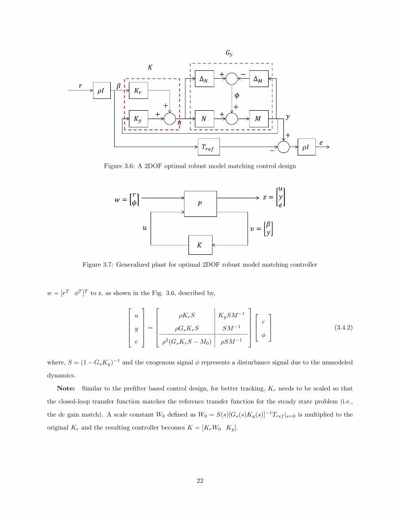
Figure 3.6: A 2DOF optimal robust model matching control design

Figure 3.7: Generalized plant for optimal 2DOF robust model matching controller

w = [rT φT ]T to z, as shown in the Fig. 3.6, described by,

u

y

e

=

ρKrS KySM

−1

ρGsKrS SM−1

ρ2(GsKrS −M0) ρSM−1

r

φ

(3.4.2)

where, S = (1−GsKy)−1 and the exogenous signal φ represents a disturbance signal due to the unmodeled

dynamics.

Note: Similar to the prefilter based control design, for better tracking, Kr needs to be scaled so that

the closed-loop transfer function matches the reference transfer function for the steady state problem (i.e.,

the dc gain match). A scale constant W0 defined as W0 = S(s)[Gs(s)Ky(s)]−1Tref |s=0 is multiplied to the

original Kr and the resulting controller becomes K = [KrW0 Ky].

22

Chapter 4

Controller Implementation on FPAAand Experimental Results

4.1 Balanced Realization and Model Reduction

A state-space realization with equal and diagonal controllability and observability gramians is called a

balanced realization [6]. Assuming the scanner system G has a state-space realization (A,B,C,D), this

realization is minimal if (A,B) is controllable and (C,A) is observable. Minimal realization is the lowest

order realization possible for a given system. The A matrix of the minimal realization is Hurwitz. Balanced

realization is obtained by applying certain state transformation to the minimal realization of the system.

A balanced system will have the controllability and observability ellipsoids exactly aligned. Thus the more

controllable states are also more observable.

Balanced realization usually comes as a precursor step of model reduction. Model reduction step elimi-

nates the least observable and controllable states by only retaining the states corresponding to larger Hankel

singular values. So, by balanced truncation technique the states with small singular values are truncated.

While following this process of model reduction it is important to keep the system input-output properties

approximately same.

Each FPAA board from Anadigm family has limited number of op-amps and is capable of implementing

only up to a maximum of eighth-order transfer function (for non-minimum phase systems, the realized order

is even lesser). Hence, model reduction is a useful tool to be able to implement reduced order controller on

a single FPAA hardware.

We now employ the control algorithms described in the previous section to the MFP-3D scanner Y-stage

(and X-stage). As described earlier, the controllers were implemented on an FPAA system. Fig. 4.1 shows

the experimental setup for controlling the nanopositioning system.

Feedback only H∞ control design and three types of 2DOF control design described in the previous

section ere applied to the MFP-3D scanner. The plant transfer functions for the Y-stage and the X-stage

are respectively,

23

Figure 4.1: Experimental setup for controlling the nanopositioning system

Gyy =0.025231(s+ 1329)(s2 + 1008s+ 1.673× 107)

(s+ 738.8)(s2 + 981.1s+ 3.574× 106)

× (s2 + 508s+ 5.426× 107)(s2 − 1.172× 104s+ 1.097× 108)

(s2 + 1213s+ 2.35× 107)(s2 + 483.8s+ 6.512× 107)(4.1.1)

Gxx =−0.022119(s+ 2.954× 104)(s+ 8117)(s− 8151)(s+ 418.9)(s2 + 890.2s+ 1.131× 107)

(s+ 1796)(s+ 217.1)(s2 + 717.5s+ 1.013× 107)(s2 + 1827s+ 3.751× 107)

× (s2 + 1185s+ 4.616× 107)(s2 + 350.3s+ 1.175× 108)(s2 + 452.4s+ 1.494× 108)

(s2 + 1440s+ 7.142× 107)(s2 + 267.1s+ 1.182× 108)(s2 + 605.8s+ 1.473× 108)(4.1.2)

4.2 1DOF H∞ control design

The H∞ optimization routine was solved for the weighting functions Ws = 0.5(s+1.257×104)(s+125.7) , Wu = 0.1, and

Wt = 58.8235(s+1257)(s+1.257×105) . This optimization resulted in a ninth-order stable controller, Kfb, with γopt = 1.9183,

Kfb =0.0077965(s+ 2096)(s+ 1.257× 105)(s+ 1.193× 109)

(s+ 2.605× 106)(s+ 3.414× 104)(s+ 125.7)

× (s2 + 206.2s+ 7.421× 105)(s2 + 550.3s+ 1.038× 107)(s2 + 87.67s+ 1.17× 107)

(s2 + 168.2s+ 8.315× 105)(s2 + 69.53s+ 1.163× 107)(s2 + 3544s+ 2.199× 107)(4.2.1)

24

Balanced truncation results in a reduced sixth-order controller given by,

Kfb =1.413(s+ 3.607× 105)(s+ 2150)(s2 + 208.1s+ 7.438× 105)(s2 + 598.5s+ 1.054× 107)

(s+ 3.972× 104)(s+ 125.7)(s2 + 168.7s+ 8.335× 105)(s2 + 3479s+ 2.233× 107)(4.2.2)

The corresponding sensitivity and complementary sensitivity transfer functions are shown in the FIg.

4.2.

Figure 4.2: Theoretical S and T for 1DOF H∞ control

Figure 4.3: Designing reduced order feedback controller on an FPAA using AnadigmDesiner2 software

25

The experimental tracking results for 100Hz sinusoidal and triangular waveforms are shown in Fig. 4.4,

(a) Tracking a 100-Hz sinusoidal reference signal

(b) Tracking a 100-Hz triangular reference signal

Figure 4.4: Tracking performance using a 1DOF H∞-control design

From Fig. 4.2, the closed-loop bandwidth is approximately 280 Hz, which is a significant improvement

in tracking bandwidth. The complementary sensitivity transfer function rolls-off at a rate of -20dB/decade,

thereby, attenuating high-frequency noise.

26

Figure 4.5: Choice of Wr and Wn weighting functions

4.3 2DOF H∞ control design

To overcome the shortcomings resulting from feedback only control, we now implement a 2DOF H∞ control

design. The performance objectives of high bandwidth, high resolution, and robustness to modeling errors

are reflected into weighting transfer functions Ws,Wu and Wt. Even though a 2DOF framework has separate

controls for reference and error signals, the fundamental algebraic limitation still holds true, S + T = 1. To

alleviate this problem even further, weighting functions Wr and Wn are used to shape reference and noise

signals respectively. The weighting functions for the 2DOF optimization problem are:

Ws =0.5(s+ 1.257× 104)

(s+ 125.7)(4.3.1)

Wu = 0.1 (4.3.2)

Wt =58.8235(s+ 1257)

(s+ 1.257× 105)(4.3.3)

Wr =1.9531(s+ 251.3)(s+ 5027)2

(s+ 628.3)2(s+ 3.142× 104)(4.3.4)

Wn = Wr−1 (4.3.5)

The choice of Wr and Wn is made such that at the frequency the Wt starts increasing, Wr starts increasing

and Wn starts decreasing (in fact Wn is chosen as the inverse of Wr). Fig. 4.5 shows the two weighting

functions.

27

The optimization routine resulted in the feedforward controller, Kff and feedback controller, Kfb with

γopt = 2.8654. Model reduction technique resulted in the following reduced-order controllers,

Kff =−2.2489(s+ 1.706× 106)(s+ 1.401× 104)(s+ 6833)(s+ 2790)(s− 6764)

(s+ 3.024× 105)(s2 + 3052s+ 4.001× 107)(s2 + 1.798× 104s+ 3.764× 108)(4.3.6)

Kfb =−0.66107(s+ 1.217× 105)(s+ 5.997× 105)(s− 9.831× 106)(s2 + 405.5s+ 3.445× 106)

(s+ 3.35× 105)(s+ 1.219× 106)(s+ 4.857× 104)(s+ 1.08× 104)(s+ 109.4)

(4.3.7)

The experimental tracking results for 100Hz sinusoidal and triangular waveforms are shown in Fig. 4.7.

Figure 4.6: S and T for mixed-sensitivty 2DOF H∞ control

Clearly, the 2DOF control design does a better job at tracking when compared to its 1DOF counter-

part. The reference and experimental trajectories are in phase, whereas, this wasn’t the case with 1DOF

setup. From Fig. 4.6, the theoretical closed-loop bandwidth is approximately 490 Hz, which is a significant

improvement in tracking bandwidth. The complementary sensitivity transfer function rolls-off at a rate of

-20dB/decade, thereby, attenuating high-frequency noise.

28



Figure 4.7: Tracking performance using a 2DOF H∞-control design

29

4.4 2DOF Model-Matching control

We now design the prefilter-based control, assuming Kfb as the pre-designed feedback component,

Kfb =−0.66107(s+ 1.217× 105)(s+ 5.997× 105)(s− 9.831× 106)(s2 + 405.5s+ 3.445× 106)

(s+ 3.35× 105)(s+ 1.219× 106)(s+ 4.857× 104)(s+ 1.08× 104)(s+ 109.4)

(4.4.1)

The NP (Nevanlinna-Pick) solution resulted in a stable prefilter, which after model-reduction and dc

gain adjustment resulted in the following sixth-order prefilter,

Kpre =0.00079405(s+ 1.217× 106)(s+ 2.804× 104)(s2 + 428.6s+ 9.935× 105)(s2 + 1965s+ 6.623× 106)

(s2 + 713.5s+ 1.192× 106)(s2 + 412s+ 3.698× 106)(s2 + 3286s+ 4.048× 107)

(4.4.2)

Fig. 4.8 shows the sensitivity and complementary transfer functions for the 2DOF model-matching

control design. The theoretical bandwidth is roughly around 240Hz.

Figure 4.8: S and T for model-matching control


The slightly poor tracking performance is attributed to the fact that the NP solution doesn’t take into

account the robustness properties of the closed-loop system.

30



Figure 4.9: Tracking performance using a 2DOF optimal prefilter based design

4.5 2DOF Optimal Robust Model Matching control

An alternative representation of the 2DOF optimal robust model matching design is shown in the Fig. 4.10.

where, W1 is the filter for shaping the plant G, and K1 is replaced by K1Wi to give exact model-matching

at steady-state. The parameters, ρ,W1 and Tref can be adjusted, if required.

31

Figure 4.10: S and T for model-matching control

4.5.1 Reduced-order controller for Y-stage

We now implement the above 2DOF H∞ loop-shaping reduced-order controller on the Y-stage. With ρ = 1

and W1 = 1, the H∞ optimization routine resulted in the following stabilizing controllers in the positive

feedback setup,

K1 =0.29483(s2 + 223.4s+ 7.538× 105)(s2 + 536.7s+ 1.063× 107)(s2 + 6.262e04s+ 1.063× 1010)

(s+ 7.195× 104)(s+ 8701)(s2 + 274.2s+ 9.724× 105)(s2 + 1959s+ 1.179× 107)

(4.5.1)

KS =−0.051402(s+ 5902)(s+ 434.7)(s2 − 1701s+ 2.723× 106)

(s2 + 299.9s+ 1.032× 106)(s2 + 1651s+ 1.386× 107)

(4.5.2)


control design. The theoretical bandwidth is roughly around 350Hz.


4.5.2 High-order controller for X-stage

Till now, we had used only limited number of FPAA resources and were therefore not able to implement

higher-order controllers. However, one can daisy chain two FPAAs together to implement higher-order

transfer function. This is achieved by connecting the output of the one FPAA to the input of the other. We

now implement higher-order 2DOF optimal robust model-matching controller for the X-stage, whose plant

32

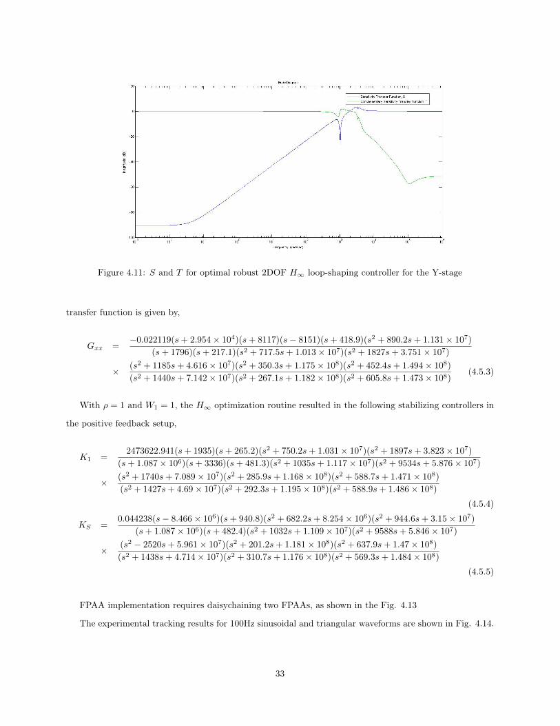
Figure 4.11: S and T for optimal robust 2DOF H∞ loop-shaping controller for the Y-stage

transfer function is given by,

Gxx =−0.022119(s+ 2.954× 104)(s+ 8117)(s− 8151)(s+ 418.9)(s2 + 890.2s+ 1.131× 107)

(s+ 1796)(s+ 217.1)(s2 + 717.5s+ 1.013× 107)(s2 + 1827s+ 3.751× 107)

× (s2 + 1185s+ 4.616× 107)(s2 + 350.3s+ 1.175× 108)(s2 + 452.4s+ 1.494× 108)

(s2 + 1440s+ 7.142× 107)(s2 + 267.1s+ 1.182× 108)(s2 + 605.8s+ 1.473× 108)(4.5.3)

With ρ = 1 and W1 = 1, the H∞ optimization routine resulted in the following stabilizing controllers in

the positive feedback setup,

K1 =2473622.941(s+ 1935)(s+ 265.2)(s2 + 750.2s+ 1.031× 107)(s2 + 1897s+ 3.823× 107)

(s+ 1.087× 106)(s+ 3336)(s+ 481.3)(s2 + 1035s+ 1.117× 107)(s2 + 9534s+ 5.876× 107)

× (s2 + 1740s+ 7.089× 107)(s2 + 285.9s+ 1.168× 108)(s2 + 588.7s+ 1.471× 108)

(s2 + 1427s+ 4.69× 107)(s2 + 292.3s+ 1.195× 108)(s2 + 588.9s+ 1.486× 108)

(4.5.4)

KS =0.044238(s− 8.466× 106)(s+ 940.8)(s2 + 682.2s+ 8.254× 106)(s2 + 944.6s+ 3.15× 107)

(s+ 1.087× 106)(s+ 482.4)(s2 + 1032s+ 1.109× 107)(s2 + 9588s+ 5.846× 107)

× (s2 − 2520s+ 5.961× 107)(s2 + 201.2s+ 1.181× 108)(s2 + 637.9s+ 1.47× 108)

(s2 + 1438s+ 4.714× 107)(s2 + 310.7s+ 1.176× 108)(s2 + 569.3s+ 1.484× 108)

(4.5.5)

FPAA implementation requires daisychaining two FPAAs, as shown in the Fig. 4.13


33



Figure 4.12: Tracking performance using a 2DOF optimal robust H∞ loopshaping control for the Y-stage

34

Figure 4.13: Daisy chaining two FPAAs to implement higher-order controller


control design. The theoretical bandwidths are ωB = 261Hz, ωBT = 850Hz.

35



Figure 4.14: Tracking performance using a 2DOF optimal robust H∞ loopshaping control for the X-stage

36

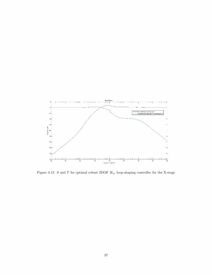
Figure 4.15: S and T for optimal robust 2DOF H∞ loop-shaping controller for the X-stage

37

Chapter 5

Q-Control of Microcantilevers

5.1 Introduction

Having demonstrated the role of the FPAAs for the nanopositioning systems, it still remains to exploit

their high-bandwidth (∼ 400kHz) capabilities for the cantilever subsystem. A cantilever is a second-order

flexible structure with very high resonant frequencies (10 − 400kHz). Controlling a cantilever system will

require hardware that can support similar bandwidth operations. In this chapter, we demonstrate the

application of an FPAA system to the Q-control of microcantilevers. Moreover, we also demonstrate the

FPAA’s capabilities to perform other complex operations [8] such as, multiplying two signals, sample and

hold operation, sine wave generation, etc.

For a similar image quality, a higher scan speed requires more information per time unit from the surface

and therefore more interaction between tip and sample is needed. Stronger tip-sample interaction poses

high Q-factor requirements on the cantilevers. Similarly, for rough/irregular samples with relatively larger

feature sizes require cantilevers with reduced sensitivities and therefore, low Q-factor.

Also, it has been established that tapping mode yields good results when the lateral positioning band-

widths are about 1%-5% of the cantilever resonant frequencies. Increasing the resonance frequency of micro-

cantilevers corresponding to increase in bandwidths of the positioning systems helps maintain the necessary

ratio between the two frequencies and provides higher speed scans [35]. Hence, high positioning band-

width (∼500Hz) would mean higher cantilever resonant frequency (∼50kHz). This poses high bandwidth

requirements on the controller for performing Q-control.

38

5.2 Velocity estimation using modulation-demodulation

approach

Cantilevers are second-order resonant structures with relatively sharper resonant frequencies (high Q-factor).

A typical cantilever dynamics from piezo input to deflection can be approximated by the following ODE:

x(t) +ωnQx(t) + ω2

nx(t) = kω2nu(t) (5.2.1)

where, k is the DC gain.

In tapping mode AFM, the cantilevers are made to oscillate at frequencies close to the resonant frequen-

cies. A typical cantilever tip deflection signal is oscillatory and is of the form,

x(t) = A cos(ω0t) +B sin(ω0t) (5.2.2)

where, ω0 ≈ ωn is the driving frequency of the cantilever.

Hence, the tip velocity is given by,

x(t) = −Aω0 sin(ω0t) +Bω0 cos(ω0t)

x(t)

ω0= −A sin(ω0t) +B cos(ω0t) (5.2.3)

Clearly, the cantilever tip velocity is orthogonal to the tip deflection signal. Hence, estimating tip velocity

is equivalent to generating orthogonal signal to the given deflection signal.

Now, supposing we have correct estimate of the cantilever tip velocity, the corresponding piezo input for

Q-factor control is given by:

u(t) = −Kvx(t)

ω0+ u(t) (5.2.4)

where, u(t) can be used to control the cantilever’s deflection

Substituting eq. 5.2.4 into cantilever dynamics, we obtain:

x(t) +ωnQeff

x(t) + ω2nx(t) = kω2

nu(t) (5.2.5)

where, Qeff =Q

1 + kKvQ(5.2.6)

39

Figure 5.1: Schematic for velocity estimation

By choosing appropriate values (both positive and negative) for the gain parameter Kv, required Q-factors

can be realized.

However, it still remains to correctly estimate the cantilever velocity. This is achieved by properly

estimating the amplitudes A and B in eq. 5.2.2 using Modulation-Demodulation, a technique mostly used

in radio transmissions. Fig. 5.1 shows the layout for velocity estimation using modulation-demodulation

operation.

The deflection signal x(t) is multiplied by corresponding sinusoidal signals to obtain in-phase and quadra-

ture components, as follows:

xIN (t) = −2x(t) sin(ω0t) = −2 {A cos(ω0t) +B sin(ω0t)} sin(ω0t)

= −A sin(2ω0t)− 2B sin2(ω0t)

= −A sin(2ω0t)−B(1− cos(2ω0t))

= −B −A sin(2ω0t) +B cos(2ω0t) (5.2.7)

40

xQ(t) = −2x(t) cos(ω0t) = −2 {A cos(ω0t) +B sin(ω0t)} cos(ω0t)

= −2A cos2(ω0t)−B sin(2ω0t)

= −A(1 + cos(2ω0t))−B sin(2ω0t)

= −A−A cos(2ω0t)−B sin(2ω0t) (5.2.8)

Clearly, the in-phase and quadrature components have not only DC components but sinusoidal components

with resonant frequency 2ω0. If we allow the individual signals to pass through a low pass filter F (s) with

cut-off frequency ωc < 0.1ω0,

F (s) =Kvωcs+ ωc

(5.2.9)

The high-frequency component gets filtered out and the amplitudes A and B are recovered. The filtered

signals are then multiplied by sin(ω0t) and − cos(ω0t) to obtain velocity estimate as:

xest(t)

ω0= −A sin(ω0t) +B cos(ω0t) (5.2.10)

Clearly, the above equations is same as eq. 5.2.3.

Figure 5.2: Implementing Modulation-Demodulation on FPAA

41

5.3 Q-control implementation on FPAA and Experimental

results

It’s now evident from the previous section that implementing Q-control not only requires a low pass fil-

ter but also accurately generating two π2 phase-shifted oscillatory periodic waveforms and multiplying two

high-frequency signals, too. Assuming that the cantilever driving frequency is roughly around 50kHz, a

typical DSP (Digital Signal Processor) hardware is not suited for Q-control, as the Nyquist limit will require

the hardware to support a minimum of 100kHz sampling frequency for all these operations. For better

implementation, even higher sampling rate is required, i.e., ∼ 400kHz (corresponds to eight data points per

cycle). This, however, can be easily achieved on an FPAA hardware, which has bandwidth up to 400kHz.

An FPAA implementation of this modulation-demodulation approach for a ∼50kHz deflection signal is

shown in the Fig. 5.2. The internal sine wave oscillator block is used to generate a 50kHz sinusoidal signal.

The differentiator block then generates an equivalent 50kHz, π2 phase-shifted signal. The modulated signal

is allowed to pass through a low-pass filter with cut-off frequency, fC = 3kHz(≈ 0.06f0). The filtered

signal is then multiplied by the phase-shifted signal. Two such FPAA boards are used to perform the two

modulation-demodulation operations. The schematic of Q-control of the cantilever is shown in the Fig. 5.3

Figure 5.3: Schematic of Q-factor control of a microcantilever

Fig. 5.4 shows the experimental validation of this modulation-demodulation Q-control approach for a

50kHz deflection signal. Using this approach, we are able to generate an orthogonal signal of the same

amplitude and frequency, thereby providing a reasonable estimate for velocity,

42

Figure 5.4: Estimating velocity using modulation-demodulation approach

43

Chapter 6

Conclusion and Future Work

The above work is a step towards the final goal of developing video-rate imaging in AFMs. This thesis

highlights not only the significance of tools from the robust control theory to design high-bandwidth, high-

resolution optimal control for nanopositioning systems, but also the direct implementation of these high-

bandwidth controllers onto an FPAA, too. Three types of 2DOF control design (optimal prefilter model

matching design, 2DOF mixed sensitivity synthesis, and 2DOF optimal robust model matching design) are

described. The experimental results show a significant improvement in tracking bandwidth and match closely

to the corresponding simulation results. With FPAAs, the achievable closed-loop nanopositioning system

bandwidth is as high as 480 Hz, which is a significant improvement over the closed-loop bandwidth (300

Hz) achieved in [5, 10]. Moreover, a twelfth-order 2DOF H∞ robust loop shaping controller for the X-stage

results in high bandwidth, high resolution tracking performance as evident form the experimental results.

We plan to extend this work with FPAAs to develop a new mode of imaging that not only exploits

the advantage with fast controllers to help achieve video-rate imaging, but also enable real-time property

estimation. This will open up new avenues to imaging biological samples. Simulations pertaining to property

estimation have been reported in [36]. We plan to exploit the capabilities of an FPAA to experimentally

demonstrate real-time property estimation.

44

References

[1] S. Hauck and A. DeHon, Reconfigurable computing: the theory and practice of FPGA-based computation.Morgan Kaufmann, 2010.

[2] S. Bains, “Analog’s answer to fpga opens field to masses,” EE Times, vol. 1510, p. 1, 2008.

[3] J.-M. Galliere, “A control-systems fpaa based tutorial,” in Proceedings of the 2nd WSEAS/IASMEInternational Conference on Educational Technologies, Bucharest, Romania, pp. 39–42, 2006.

[4] N. Kodera, D. Yamamoto, R. Ishikawa, and T. Ando, “Video imaging of walking myosin v by high-speedatomic force microscopy,” Nature, vol. 468, no. 7320, pp. 72–76, 2010.

[5] C. Lee and S. M. Salapaka, “Robust broadband nanopositioning: fundamental trade-offs, analysis, anddesign in a two-degree-of-freedom control framework,” Nanotechnology, vol. 20, no. 3, p. 035501, 2009.

[6] G. Dullerud and F. Paganini, Course in Robust Control Theory. Springer-Verlag New York, 2000.

[7] S. Skogestad and I. Postlethwaite, Multivariable feedback control: analysis and design, vol. 2. WileyNew York, 2007.

[8] F. Anadigm, “Family overview,” PDF File, Anadigm, 2003.

[9] T. Sulchek, R. Hsieh, J. Adams, G. Yaralioglu, S. Minne, C. Quate, J. Cleveland, A. Atalar, andD. Adderton, “High-speed tapping mode imaging with active q control for atomic force microscopy,”Applied Physics Letters, vol. 76, no. 11, pp. 1473–1475, 2000.

[10] C. Lee, S. M. Salapaka, and P. G. Voulgaris, “Two degree of freedom robust optimal control designusing a linear matrix inequality optimization,” in Decision and Control, 2009 held jointly with the2009 28th Chinese Control Conference. CDC/CCC 2009. Proceedings of the 48th IEEE Conference on,pp. 714–719, IEEE, 2009.

[11] S. Mashrafi, C. Preissner, S. Salapaka, and H. Zhao, “Something for (almost) nothing: X-ray microscopeperformance enhancement through control architecture change,” in ASPE 28th Annual Meeting, 2013.

[12] S. M. Salapaka and M. V. Salapaka, “Scanning probe microscopy,” Control Systems, IEEE, vol. 28,no. 2, pp. 65–83, 2008.

[13] G. Schitter and N. Phan, “Field programmable analog array (fpaa) based control of an atomic forcemicroscope,” in American Control Conference, 2008, pp. 2690–2695, IEEE, 2008.

[14] K. Glover and D. McFarlane, “Robust stabilization of normalized coprime factor plant descriptionswith H∞-bounded uncertainty,” Automatic Control, IEEE Transactions on, vol. 34, no. 8, pp. 821–830,1989.

[15] Q. Zhong, D. Inniss, K. Kjoller, and V. Elings, “Fractured polymer/silica fiber surface studied bytapping mode atomic force microscopy,” Surface Science Letters, vol. 290, no. 1, pp. L688–L692, 1993.

45

[16] T. S. Hall, C. M. Twigg, P. Hasler, and D. V. Anderson, “Application performance of elements in afloating-gate fpaa,” in Circuits and Systems, 2004. ISCAS’04. Proceedings of the 2004 InternationalSymposium on, vol. 2, pp. II–589, IEEE, 2004.

[17] R. Selow, H. S. Lopes, and C. Lima, “A comparison of fpga and fpaa technologies for a signal processingapplication,” in Field Programmable Logic and Applications, 2009. FPL 2009. International Conferenceon, pp. 230–235, IEEE, 2009.

[18] Field Programmable Analog Array: AN231K04-DVLP3 - AnadigmApex Development Board. AnadigmInc., Campbell, CA, USA, 2006.

[19] L. Ljung, “System identification: theory for the user,” Preniice Hall Inf and System Sciencess Series,New Jersey, vol. 7632, 1987.

[20] G. Mohan, A new dynamic mode for fast imaging in atomic force microscopes. PhD thesis, Universityof Illinois at Urbana-Champaign, 2013.

[21] D. Croft, G. Shed, and S. Devasia, “Creep, hysteresis, and vibration compensation for piezoactuators:atomic force microscopy application,” Journal of Dynamic Systems, Measurement, and Control, vol. 123,no. 1, pp. 35–43, 2001.

[22] A. G. Hatch, R. C. Smith, T. De, and M. V. Salapaka, “Construction and experimental implementationof a model-based inverse filter to attenuate hysteresis in ferroelectric transducers,” Control SystemsTechnology, IEEE Transactions on, vol. 14, no. 6, pp. 1058–1069, 2006.

[23] B. Bhikkaji, M. Ratnam, A. J. Fleming, and S. R. Moheimani, “High-performance control of piezoelec-tric tube scanners,” Control Systems Technology, IEEE Transactions on, vol. 15, no. 5, pp. 853–866,2007.

[24] A. Daniele, S. Salapaka, M. Salapaka, and M. Dahleh, “Piezoelectric scanners for atomic force micro-scopes: Design of lateral sensors, identification and control,” in American Control Conference, 1999.Proceedings of the 1999, vol. 1, pp. 253–257, IEEE, 1999.

[25] S. Salapaka, A. Sebastian, J. P. Cleveland, and M. V. Salapaka, “High bandwidth nano-positioner: Arobust control approach,” Review of scientific instruments, vol. 73, no. 9, pp. 3232–3241, 2002.

[26] K. K. Leang and S. Devasia, “Hysteresis, creep, and vibration compensation for piezoactuators: Feed-back and feedforward control,” in Proceedings of the Second IFAC Conference on Mechatronic Systems,Berkeley, CA, Dec, pp. 9–11, 2002.

[27] G. Schitter, F. Allgower, and A. Stemmer, “A new control strategy for high-speed atomic force mi-croscopy,” Nanotechnology, vol. 15, no. 1, p. 108, 2004.

[28] Q. Zou and S. Devasia, “Preview-based optimal inversion for output tracking: Application to scanningtunneling microscopy,” Control Systems Technology, IEEE Transactions on, vol. 12, no. 3, pp. 375–386,2004.

[29] J. C. Doyle, B. A. Francis, and A. Tannenbaum, Feedback control theory, vol. 1. Macmillan PublishingCompany New York, 1992.

[30] A. Sebastian and S. M. Salapaka, “Design methodologies for robust nano-positioning,” Control SystemsTechnology, IEEE Transactions on, vol. 13, no. 6, pp. 868–876, 2005.

[31] D. McFarlane and K. Glover, “A loop-shaping design procedure using H∞ synthesis,” Automatic Con-trol, IEEE Transactions on, vol. 37, no. 6, pp. 759–769, 1992.

[32] D. Hoyle, R. Hyde, and D. Limebeer, “An H∞ approach to two degree of freedom design,” in Decisionand Control, 1991., Proceedings of the 30th IEEE Conference on, pp. 1581–1585, IEEE, 1991.

46

[33] D. J. Limebeer, E. Kasenally, and J. Perkins, “On the design of robust two degree of freedom controllers,”Automatica, vol. 29, no. 1, pp. 157–168, 1993.

[34] M. Vidyasagar, Control system synthesis: a facotrization approach. Morgan & Claypool Publishers,2011.

[35] D. Walters, J. Cleveland, N. Thomson, P. Hansma, M. Wendman, G. Gurley, and V. Elings, “Shortcantilevers for atomic force microscopy,” Review of Scientific Instruments, vol. 67, no. 10, pp. 3583–3590,1996.

[36] S. M Salapaka, T. De, and A. Sebastian, “A robust control based solution to the sample-profile estima-tion problem in fast atomic force microscopy,” International Journal of Robust and Nonlinear Control,vol. 15, no. 16, pp. 821–837, 2005.

47

2014 mayank baranwal.web.engr.illinois.edu/~salapaka/pdfs/pdfs/baranwal2014...application of field...

Documents