2015 natural gas demand side management annual ... · ontario gas dsm evaluation contractor 2015...
TRANSCRIPT

ONTARIO GAS DSM EVALUATION CONTRACTOR
2015 Natural Gas Demand Side Management Annual Verification Ontario Energy Board
Date: December 20, 2017

DNV GL – www.dnvgl.com Page i

DNV GL – www.dnvgl.com Page ii
Table of Contents
TABLE OF CONTENTS ................................................................................................................ II
1 Executive Summary ...................................................................................................... 1 1.1 Method summary 1 1.2 Results 2 1.3 2015 annual verification recommendations 5
2 Introduction ............................................................................................................... 10 2.1 Background 10 2.2 Method summary 11
3 Union Gas Limited ....................................................................................................... 14 3.1 Scorecard achievements 14 3.2 Program spending and cost-effectiveness 20 3.3 DSMSI and LRAM 21
4 Enbridge Gas Distribution, Inc. ..................................................................................... 25 4.1 Scorecard achievements 25 4.2 Program spending and cost-effectiveness 31 4.3 DSMSI and LRAM 32
5 Findings and recommendations ..................................................................................... 36 5.1 2015 annual verification recommendations 36 5.2 CPSV / NTG findings and recommendations 43
APPENDIX A. DATA AND DOCUMENTATION REQUESTS .............................................................. A-1
APPENDIX B. DESCRIPTION OF DATA RECEIVED ...................................................................... B-1
APPENDIX C. PRESCRIPTIVE SAVINGS VERIFICATION ............................................................... C-1
APPENDIX D. RESIDENTIAL RETROFIT PROGRAM VERIFICATION ................................................. D-1
APPENDIX E. ENERGY SAVINGS KIT VERIFICATION .................................................................. E-1
APPENDIX F. RUNITRIGHT VERIFICATION ............................................................................... F-1
APPENDIX G. LOW INCOME MULTI-FAMILY VERIFICATION ......................................................... G-3
APPENDIX H. CUSTOM PROJECT VERIFICATION ........................................................................ H-4
APPENDIX I. MARKET TRANSFORMATION VERIFICATION ........................................................... I-1
APPENDIX J. REVIEW OF LRAM AND DSMSI CALCULATIONS .......................................................J-1
APPENDIX K. LRAM AND DSMSI: DETAILED CALCULATIONS ....................................................... K-1
APPENDIX L. PROGRAM SPENDING ........................................................................................ L-1

DNV GL – www.dnvgl.com Page iii
APPENDIX M. COST-EFFECTIVENESS METHODOLOGY ............................................................... M-1
APPENDIX N. SPILLOVER ESTIMATE ........................................................................................ N-1
APPENDIX O. FINAL ANNUAL VERIFICATION EM&V PLAN ........................................................... O-1
APPENDIX P. FINAL CPSV/NTG REPORT ................................................................................... P-1

DNV GL – www.dnvgl.com Page i
AUDIT OPINION The Evaluation Contractor team (DNV GL, Itron, and Dunsky) provides the following opinion on the utility-achieved savings, lost revenue, and shareholder incentive for the calendar year ended December 31, 2015. Our opinion stems from our review of the program documentation, utility shareholder incentive calculations, and lost revenue calculations as set forth in the report that follows. It is also based on the information available at the time that this report was published.
In our opinion, the following figures are reasonable, subject to the qualifications given above.
Definition Union Result Enbridge Result
Shareholder Incentive $7,039,894 $6,207,339
Lost Revenue $154,368 $16,405
Verified Net Cumulative Savings 1,137,825,562 m3 539,787,741 m3
Total Dollars Spent (not reviewed) $32,178,766 $35,779,973
Cost Effectiveness (TRC test) 2.9 2.2

DNV GL – www.dnvgl.com Page 1
1 Executive Summary This document has been prepared for the Ontario Energy Board (OEB) and outlines the results of the annual verification of Enbridge Gas Distribution Inc.’s (Enbridge) and Union Gas Limited’s (Union) natural gas demand-side management (DSM) programs1 delivered in 2015. These verifications were conducted by the Evaluation Contractor (EC) team.
The annual verification assembles the results of all evaluation studies conducted on the 2015 programs and applies them to the savings and scorecard metrics reported by the utilities. For programs or metrics where no recent studies have been performed, the EC team conducts a due diligence review to verify the savings or metrics reported by the utilities.
The overall objectives of the evaluations are to:
Provide an independent opinion on whether the Lost Revenue Adjustment Mechanism (LRAM), DSM Variance Account (DSMVA), and DSM Shareholder Incentive (DSMSI) have been calculated correctly using the most appropriate information.
Recommend future evaluation research opportunities to enhance the future natural gas savings estimates and other assumptions used to calculate DSMSI and LRAM amounts.
Recommend changes to improve input assumptions, verification procedures, and the overall verification process.
1.1 Method summary To verify the utility scorecard metrics discussed in the following sections, the EC conducted the activities listed below. To prepare for the program-specific activities, the EC requested tracking data and, where necessary, documentation for a sample of projects or participants from the utilities. The EC completed program-specific verifications and used the results to calculate the DSMSI and LRAM for both Enbridge and Union. We also calculated cost-effectiveness and reported program spending. The verification activities included:
Custom project savings: Apply the results of the completed custom project savings verification (CPSV) of custom commercial, industrial, and Large Volume programs, which included a free ridership component, and include a provisional estimate for spillover.
Prescriptive project savings: Confirm that the measure-level inputs for prescriptive measures were appropriate and confirm that the savings were calculated correctly for the full population of measures.
Residential home retrofit projects: Verify the savings for a sample of participants.
RunitRight projects: Verify the savings for a sample of participants.
Market transformation projects: Confirm participation status and program qualification for all non-savings metrics.
1 Throughout this report, the word “program” is used to reflect the OEB’s understanding of a program. The utilities define it differently. See
APPENDIX M for additional detail.

DNV GL – www.dnvgl.com Page 2
Other projects: Confirm the number of residential deep savings participants, the percent of C&I whole-building energy use saved by C&I program participants for Union, and the percent of Part 3 Low Income participants in the Low Income Building Management Performance program for Enbridge.
1.2 Results Table 1-1, Table 1-2, and Table 1-3 show the Union verified savings, DSMSI, and LRAM results, respectively. Table 1-4 shows the cost-effectiveness ratio results for Union, and Table 1-5 shows the net present value for Union. Table 1-6 through Table 1-10 show the same information for Enbridge. All utility-defined programs pass the TRC, TRC-Plus, and PAC tests.
Table 1-1. Union verified savings results Program Draft Utility-Reported Savings* Verification Results Verified Savings
Gross
Cumulative (m3)
Net Cumulative
(m3)
Gross Realization
Rate†
Net-to-
Gross†
Gross Cumulative (m3)
Net Cumulative
(m3)
Resource Acquisition Home Reno Rebate 69,321,370 58,923,165 98% 85% 67,934,943 57,744,701
Energy Savings Kit 22,398,052 19,567,373 75% 88% 16,882,059 14,800,935
Total Residential 91,719,422 78,490,538 92% 86% 84,817,002 72,545,636
C&I Custom 1,473,918,718 678,002,610 98% 44% 1,443,912,081 635,817,233
C&I Prescriptive 208,919,006 182,411,887 100% 87% 208,919,006 182,411,887
Total C&I 1,682,837,724 860,414,497 98% 50% 1,652,831,087 818,229,120 Total Resource Acquisition 1,774,557,146 938,905,035 98% 51% 1,737,648,089 890,774,755
Large Volume
Large Volume 1,253,971,028 578,023,195 135% 12% 1,691,806,721 194,870,020 Total Large Volume 1,253,971,028 578,023,195 135% 12% 1,691,806,721 194,870,020
Low Income Single Family (Part 9) 33,505,239 33,504,841 107% 100% 35,847,824 35,847,426
Multi-family (Part 3) 17,840,732 16,948,695 96% 95% 17,193,011 16,333,361
Total Low Income 51,345,970 50,453,536 103% 98% 53,040,835 52,180,787
* The utility-reported values reflect the savings presented in the utility’s tracking workbook, not in the draft 2015 report. The utility changed the energy savings values for some projects after submitting the 2015 report but before delivering the data for evaluation, resulting in a small change.
†These values are rounded.
Table 1-2. Union DSMSI results Scorecard Draft Utility-Reported DSMSI* DSMSI
Resource Acquisition $4,776,312 $4,010,638
Low Income $2,192,257 $2,462,534
Large Volume $0 $0
Market Transformation $566,721 $566,721
Total $7,535,290 $7,039,894 * The utility-reported values reflect the savings presented in the utility’s tracking workbook, not in the draft 2015 report. The utility changed the
energy savings values for some projects after submitting the 2015 report but before delivering the data for evaluation, resulting in a small change.

DNV GL – www.dnvgl.com Page 3
Table 1-3. Union LRAM results
Rate Class Utility-Reported Draft LRAM Verified LRAM
M4 Industrial $77,105 $74,681
M5 Industrial $38,366 $36,890
M7 Industrial $33,512 $32,272
T1 Industrial $2,789 $1,462
T2 Industrial $1,050 $361
20 Industrial $7,002 $6,808
100 Industrial $5,578 $1,894
Total $165,411 $154,368
Table 1-4. Union summary of cost-effectiveness ratio results
Scorecard
Draft using Utility-Reported Savings* Final Verified Ratio
TRC TRC-Plus** PAC** TRC TRC-Plus PAC
Residential Resource Acquisition 1.2 3.0 8.0
1.0 1.2 2.3
Commercial and Industrial Resource Acquisition 2.9 3.3 3.8 12.0
Low Income 1.0 1.1 0.9 1.3 1.4 1.1
Large Volume 4.7 5.4 26.3 6.0 6.9 10.2
Total Portfolio 2.9 3.3 8.1 2.9 3.3 6.8 * The utility-reported values reflect the savings presented in the utility’s tracking workbook, not in the draft 2015 report. The utility changed the
energy savings values for some projects after submitting the 2015 report but before delivering the data for evaluation, resulting in a small change. **These values were calculated using the utility-reported draft savings results for the entire Resource Acquisition scorecard. Union only reported TRC
in its filings for 2015.
Table 1-5. Union summary of cost-effectiveness net present value results
Scorecard
Draft Net Present Value (M$) using Utility-Reported Savings*
Final Verified Net Present Value (M$)
TRC TRC-Plus** PAC** TRC TRC-Plus PAC
Residential Resource Acquisition 96.7 120.4 117.9
0.4 2.6 6.8
Commercial and Industrial Resource Acquisition 105.4 128.0 124.7
Low Income (0.02) 1.0 (1.1) 1.7 3.1 0.6
Large Volume 70.2 83.6 81.1 27.6 32.6 29.4
Total Portfolio 166.9 205.1 197.9 135.2 166.3 161.5 * The utility-reported values reflect the savings presented in the utility’s tracking workbook, not in the draft 2015 report. The utility changed the
energy savings values for some projects after submitting the 2015 report but before delivering the data for evaluation, resulting in a small change. **These values were calculated using the utility-reported draft savings results. Union only reported TRC in its filings for 2015.

DNV GL – www.dnvgl.com Page 4
Table 1-6. Enbridge verified savings results
Program
Draft Utility-Reported Savings* Verification Results Verified Savings Gross
Cumulative (m3)
Net Cumulative (m3)
Gross Realization Rate**†
Net-to-Gross†
Gross Cumulative
(m3)
Net Cumulative
(m3) Resource Acquisition Home Energy Conservation 120,488,487 102,415,214 100% 85% 120,488,487 102,415,214
Total Residential 120,488,487 102,415,214 100% 85% 120,488,487 102,415,214
C&I Custom 812,730,242 558,925,884 95% 31% 773,928,967 240,326,475 C&I Prescriptive 128,765,764 106,286,730 98% 84% 125,724,435 105,009,436
Total C&I 941,496,006 665,212,614 96% 38% 899,653,401† 345,335,910† Total Resource Acquisition
1,061,984,493 767,627,826 96% 44% 1,020,141,888 447,751,124
Low Income Single Family (Part 9) 28,410,725 28,343,978 99% 100% 28,067,263 28,067,263
Multi-family (Part 3) 69,505,240 69,226,782 92% 100% 63,969,354 63,969,354
Total Low Income 97,915,965 97,570,759 94% 100% 92,036,617 92,036,617
* The utility-reported values reflect the savings presented in the utility’s tracking workbook, not in the draft 2015 report. The utility changed the energy savings values for some projects after submitting the 2015 report but before delivering the data for evaluation, resulting in a small change.
†These values are rounded. ** The gross realization rate for C&I prescriptive, single family low income, and multi-family low income includes the removal rate for some measures,
which was previously included in the net-to-gross adjustment. See APPENDIX C for more detail.
Table 1-7. Enbridge DSMSI results Scorecard Draft Utility-Reported DSMSI* DSMSI
Resource Acquisition $6,482,744 $2,612,431
Low Income $1,724,691 $1,483,748
Residential Savings by Design $1,076,493 $1,076,493
Commercial Savings by Design $418,269 $418,269
Home Labelling $616,397 $616,397
Total $10,318,594 $6,207,339 * The utility-reported values reflect the savings presented in the utility’s tracking workbook, not in the draft 2015 report. The utility changed the
energy savings values for some projects after submitting the 2015 report but before delivering the data for evaluation, resulting in a small change.
Table 1-8. Enbridge LRAM results
Rate Class Draft Utility-Reported LRAM* LRAM
110 $18,795 $11,769
115 $6,478 $2,932
135 $330 $239
145 $2,267 $876
170 $953 $590
Total $28,822 $16,405 * The utility-reported values reflect the savings presented in the utility’s tracking workbook, not in the draft 2015 report. The utility changed the
energy savings values for some projects after submitting the 2015 report but before delivering the data for evaluation, resulting in a small change.

DNV GL – www.dnvgl.com Page 5
Table 1-9. Enbridge summary of cost-effectiveness ratio results
Scorecard Draft using Utility-Reported Savings* Final Verified Ratio
TRC** TRC-Plus PAC TRC TRC-Plus PAC
Resource Acquisition 3.3 3.8 6.0 2.3 2.7 2.7
Low Income 2.1 2.5 2.5 1.6 1.9 1.7
Total Portfolio 3.1 3.6 5.2 2.2 2.5 2.5 * The utility-reported values reflect the savings presented in the utility’s tracking workbook, not in the draft 2015 report. The utility changed the
energy savings values for some projects after submitting the 2015 report but before delivering the data for evaluation, resulting in a small change. **These values were calculated using the utility-reported draft savings results. Enbridge only reported TRC-Plus and PAC in its filings for 2015.
Table 1-10. Enbridge summary of cost-effectiveness net present value results
Scorecard Draft Net Present Value (M$) using
Utility-Reported Savings* Final Verified Net Present Value (M$)
TRC** TRC-Plus PAC TRC TRC-Plus PAC
Resource Acquisition 123.2 149.7 120.4 49.9 61.5 40.7
Low Income 9.2 11.8 10.7 5.0 7.0 5.2
Total Portfolio 132.4 161.6 131.1 54.9 68.5 45.9 * The utility-reported values reflect the savings presented in the utility’s tracking workbook, not in the draft 2015 report. The utility changed the
energy savings values for some projects after submitting the 2015 report but before delivering the data for evaluation, resulting in a small change. **These values were calculated using the utility-reported draft savings results. Enbridge only reported TRC-Plus and PAC in its filings for 2015.
1.3 2015 annual verification recommendations This section contains a summary of the recommendations from the EC’s 2015 annual verification efforts, shown in the tables below. In the tables, the primary outcomes of the recommendation are classified into three categories: reduce costs (evaluation or program or both), improve savings accuracy, and decrease risk (multiple types of risk are in this category including risk of adjusted savings, risk to budgets or project schedules, and others). The complete findings, recommendations, and outcomes of the 2015 annual verification efforts and other evaluations conducted on 2015 programs are found in section 5.

DNV GL – www.dnvgl.com Page 6
Table 1-11. Summary of recommendations that apply to the overall annual verification
#
Overall Annual Verification
Recommendation
Applies to Primary Outcome
Un
ion
Enb
rid
ge
Eval
uat
ion
Red
uce
Cos
ts
Imp
rove
Sav
ing
s
Acc
ura
cy
Dec
reas
e
Ris
k
O1A Consider investing in a relational program
tracking database.
O1B Enbridge should include site-level information
for all measures installed through the
program.
O2A Deliver tracking data in a single flat file.
O2B Consider investing in a relational program
tracking database.
O3A Develop and maintain an electronic summary
of the TRM.
O3B Track prescriptive savings using unique
measure descriptions that map to electronic
TRM.
DNV GL – www.dnvgl.com Page 7
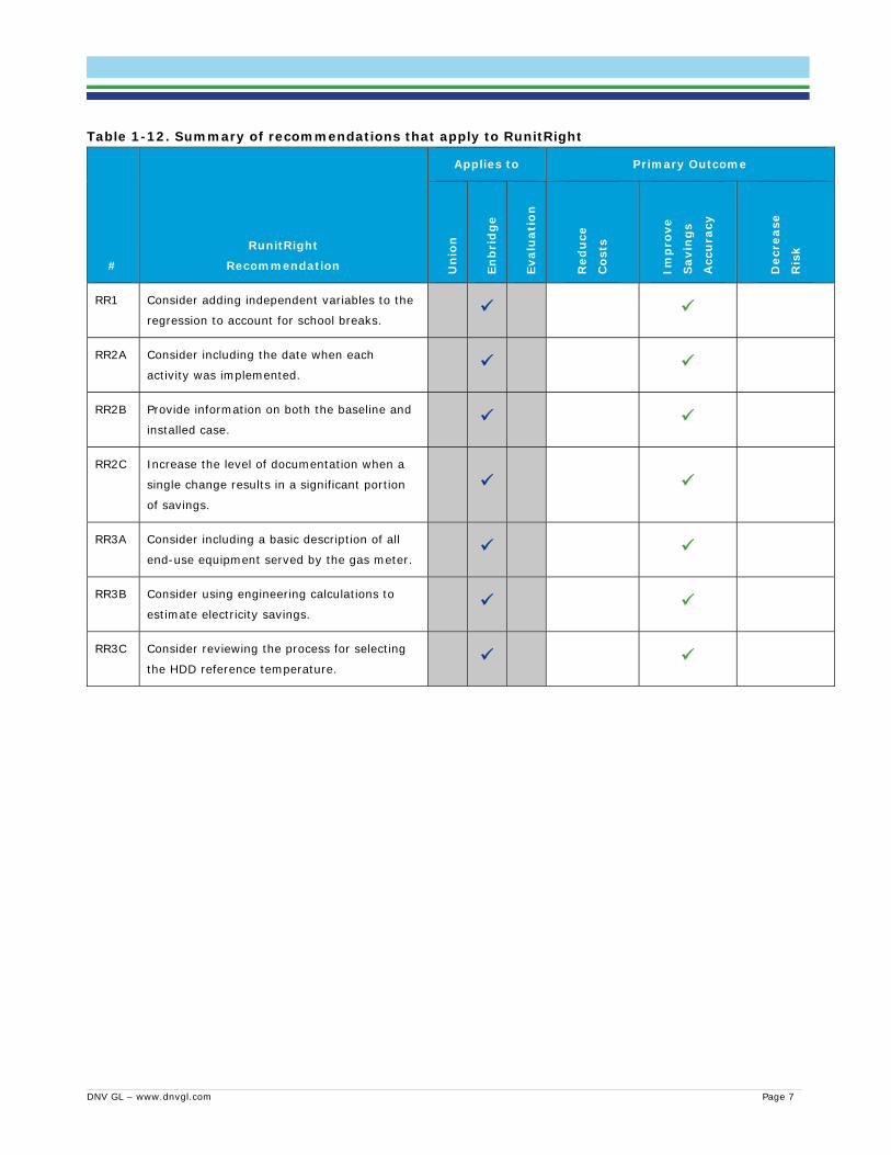
Table 1-12. Summary of recommendations that apply to RunitRight
#
RunitRight
Recommendation
Applies to Primary Outcome
Un
ion
Enb
rid
ge
Eval
uat
ion
Red
uce
Cos
ts
Imp
rove
Sav
ing
s
Acc
ura
cy
Dec
reas
e
Ris
k
RR1 Consider adding independent variables to the
regression to account for school breaks.
RR2A Consider including the date when each
activity was implemented.
RR2B Provide information on both the baseline and
installed case.
RR2C Increase the level of documentation when a
single change results in a significant portion
of savings.
RR3A Consider including a basic description of all
end-use equipment served by the gas meter.
RR3B Consider using engineering calculations to
estimate electricity savings.
RR3C Consider reviewing the process for selecting
the HDD reference temperature.

DNV GL – www.dnvgl.com Page 8
Table 1-13. Summary of recommendations that apply to simulation modeling
#
Simulation Modeling
Recommendation
Applies to Primary Outcome
Un
ion
Enb
rid
ge
Eval
uat
ion
Red
uce
Cos
ts
Imp
rove
Sav
ing
s
Acc
ura
cy
Dec
reas
e
Ris
k
SM1 Provide simulation file and output to the
evaluation team.
SM2 Provide more explicit support for major
measure installations.
SM3 Consider reviewing and modifying program
processes to avoid data entry or outdated
simulation result errors.
SM4 Consider funding a study to verify the models
produced by the utility agents.
Table 1-14. Summary of recommendations that apply to cost-effectiveness
#
Cost-effectiveness Recommendation
Applies to Primary Outcome
Un
ion
Enb
rid
ge
Eval
uat
ion
Red
uce
Cos
ts
Imp
rove
Sav
ing
s
Acc
ura
cy
Dec
reas
e
Ris
k CE1 Allocate “sector”-level administrative costs
and overhead to each individual program and
report program-level cost-effectiveness
results.
CE2 Use a consistent real discount rate of 4%
when using real streams of benefits and
costs.
CE3 Explore the possibility of better defining water
avoided costs.
CE4 Work towards better uniformity in methods
and assumptions.

DNV GL – www.dnvgl.com Page 9
Table 1-15. Summary of recommendations that apply to other areas
#
Other
Recommendation
Applies to Primary Outcome
Un
ion
Enb
rid
ge
Eval
uat
ion
Red
uce
Cos
ts
Imp
rove
Sav
ing
s
Acc
ura
cy
Dec
reas
e
Ris
k
OR1 When the C&I deep savings metric is used,
deliver monthly billing data for each C&I
participant.
OR2 Provide a detailed explanation for the DSMSI
calculation.

DNV GL – www.dnvgl.com Page 10
2 Introduction This document has been prepared for the Ontario Energy Board (OEB) and outlines the results of the annual verification of Enbridge Gas Distribution Inc.’s (Enbridge) and Union Gas Limited’s (Union) natural gas demand side management (DSM) programs2 delivered in 2015. These verifications were conducted by the OEB’s Evaluation Contractor (EC) team of DNV GL, Itron, and Dunsky.
The annual verification assembles the results of all evaluation studies conducted on the 2015 programs and applies them to the savings and scorecard metrics reported by the utilities. For programs or metrics where no recent studies have been performed, the EC team conducts a due diligence review to verify the savings or metrics reported by the utilities.
The overall objectives of the evaluations are to:
Provide an independent opinion on whether the Lost Revenue Adjustment Mechanism (LRAM), DSM Variance Account (DSMVA), and DSM Shareholder Incentive (DSMSI) have been calculated correctly using the most appropriate information.
Recommend future evaluation research opportunities to enhance the future natural gas savings estimates and other assumptions used to calculate DSMSI and LRAM amounts.
Recommend changes to improve input assumptions, verification procedures, and the overall verification process.
The LRAM, DSMVA, and DSMSI are based on the following metrics:
LRAM: the verified natural gas energy savings (in annual cubic meters) by rate class and the cost (the delivery rate) of the natural gas by rate class for the program year.
DSMVA: the actual money collected, by rate class, for implementing DSM programs during the program year and the actual DSM costs incurred by the programs.
DSMSI: the actual program achievements compared to the scorecard metrics for that program, the weight placed on each metric within each scorecard, and the maximum incentive achievable for that scorecard.
Therefore, the information that was verified for 2015 includes the program natural gas savings and the program achievements compared to the scorecard metrics. The EC also reported the money spent by the programs but did not conduct a full financial audit of the reported amounts. The OEB may conduct financial audits of the gas utilities DSM spending as it sees fit. The verified savings and program achievements were used to confirm the LRAM and DSMSI amounts.
2.1 Background Enbridge and Union deliver energy efficiency programs under the Demand Side Management Framework for Natural Gas Distributors (2015-2020)3 developed by the OEB. For the 2015 program year, both utilities “rolled-over” their 2014 plans into 2015 to allow them a smooth evolution into the new DSM framework.
2 Throughout this report, the word “program” is used to reflect the OEB’s understanding of a program. The utilities define it differently. See
APPENDIX M for additional detail. 3 EB-2014-0134

DNV GL – www.dnvgl.com Page 11
In April 2016, the OEB hired the EC team to develop an overall evaluation, measurement, and verification (EM&V) plan and lead an annual verification of the reported utility DSM achievements. This report is a result of that annual verification.
Under the EM&V plan, a DNV GL-led team of DNV GL, Itron, and Stantec conducted a custom project savings verification (CPSV) and net-to-gross (NTG) study of the 2015 program year.4 This report includes the results of that study. A spillover study of 2013-2014 programs has also been initiated; however, the results from that effort are not available for this report. Instead, a provisional value has been included in the NTG value based on secondary source research. See APPENDIX N for more information.
The OEB formed an evaluation advisory committee (EAC) to provide input and advice to the OEB and the EC on the evaluation and audit of DSM results. The EAC consists of representatives from the utilities, non-utility stakeholders, independent experts, staff from the Independent Electricity System Operator (IESO), and observers from the Environmental Commissioner of Ontario and the Ministry of Energy. The DNV GL team received feedback from the EAC throughout the CPSV/NTG study5 and received comment, advice, and input on the results of this annual verification. We thank them for their involvement.
2.2 Method summary To verify the utility scorecard metrics discussed in the following sections, the EC conducted the activities outlined in Table 2-1 and Table 2-2. To prepare for the program-specific activities, the EC requested tracking data and, where necessary, documentation for a sample of projects or participants from the utilities. For all programs, the EC first reviewed the reported savings and metrics from the gas utilities’ tracking data and compared them to the summarized information in the gas utilities’ draft annual report to ensure consistency. We also recreated the reported LRAM and DSMSI values using the reported savings and scorecard achievements to confirm that the calculations were done correctly.
Once the program-specific verifications were completed, the EC assembled the verified scorecard results and calculated the verified LRAM, DSMSI, and cost-effectiveness results. We also documented recommendations that may improve the annual verification process going forward. The full annual verification EM&V plan is embedded in APPENDIX N. The results presented in this report are based on data collected from:
Union and Enbridge tracking databases (Round 1 of data requests)
Union and Enbridge project documentation (Round 2 of data requests)
The results of the CPSV / NTG study
The two data and documentation requests are explained in detail in APPENDIX A. A description of the data received is explained in detail in APPENDIX B. The recommendations related to these activities are listed in section 5.
4 “2015 Natural Gas Demand Side Management Custom Savings Verification and Free-ridership Evaluation”. Prepared for the Ontario Energy Board.
August 15, 2017. 5 Throughout the rest of this report, “CPSV/NTG” is used to refer to the study that resulted in custom program savings verification and net-to-gross
results; however, not all aspects of the study were applied to all programs in the study. The Low Income participants were not included in the NTG portion of the study; pre-stipulated NTG results continue to be used for those measures. The Run it Right participants were not included in the CPSV portion of the study; verified gross savings were produced during the annual verification.

DNV GL – www.dnvgl.com Page 12
Table 2-1. Union 2015 annual verification activities, by scorecard
Program Metrics Activity
Res
ourc
e A
cqu
isit
ion
Cumulative natural gas savings
Number of residential deep savings participants
Average percent of whole building energy use saved by the program
Confirm that the measure-level inputs for prescriptive measures were appropriate and confirm that the savings were calculated correctly for the full population of measures.
Verify the savings for a sample of home retrofit participants.
Confirm that the necessary factors (such as NTG assumptions) were applied correctly.
Apply the results of the CPSV / NTG study.
Verify the number of residential deep savings participants by reviewing the detailed documentation for a sample of participants.
Collect the annual billing information for the full population of C&I deep savings participants and compare the verified energy savings to the annual energy use to confirm the percent of whole building natural gas use saved.
Larg
e V
olu
me
Cumulative natural gas savings
Confirm that the necessary factors (such as NTG assumptions) were applied correctly.
Confirm that the measure-level inputs for prescriptive measures were appropriate and confirm that the savings were calculated correctly for the full population of measures.
Apply the results of the CPSV / NTG study.
Low
In
com
e
Cumulative natural gas savings Confirm that the measure-level inputs for prescriptive measures were appropriate and confirm that the savings were calculated correctly for the full population of measures.
Verify the savings for a sample of home retrofit participants.
Confirm that the necessary factors (such as NTG assumptions) were applied correctly.
Apply the results of the CPSV / NTG study.
Op
tim
um
H
ome
Percent of homes built by participating builders that are 20% more efficient than OCB
Review the program tracking data.
Confirm the participation status of one builder, and confirm the program qualification of one home.

DNV GL – www.dnvgl.com Page 13
Table 2-2. Enbridge 2015 annual verification activities, by scorecard
Program Metrics Activity
Res
ourc
e A
cqu
isit
ion
Cumulative natural gas savings
Number of residential deep savings participants
Confirm that the measure-level inputs for prescriptive measures were appropriate and confirm that the savings were calculated correctly for the full population of measures.
Verify the savings for a sample of home retrofit participants.
Confirm that the necessary factors (such as NTG assumptions) were applied correctly.
Apply the results of the CPSV / NTG study.
Conduct a desk review of a sample of RunitRight participants to verify the reasonableness of the claimed savings.
Verify the number of residential deep savings participants by reviewing the detailed documentation for a sample of participants.
Low
In
com
e
Cumulative natural gas savings
Percent of Part 3 participants enrolled
Confirm that the measure-level inputs for prescriptive measures were appropriate and confirm that the savings were calculated correctly for the full population of measures.
Verify the savings for a sample of home retrofit participants.
Confirm that the necessary factors (such as NTG assumptions) were applied correctly.
Apply the results of the CPSV / NTG study.
Review documentation to confirm the Part 3 participant Low Income scorecard metric.
RS
BD
Builders enrolled
Number of efficient homes
Review the program tracking data.
Confirm the participation status of one residential builder and the program qualification of one home.
CS
BD
Number of developments Review the program tracking data.
Confirm the participation status of one commercial builder and the program qualification of one development.
Hom
e La
bel
ling
Number of listings represented by realtors
Number of ratings performed
Review the program tracking data.
Confirm the participation status of one realtor, and the ratings reported by that realtor.
DNV GL – www.dnvgl.com Page 14
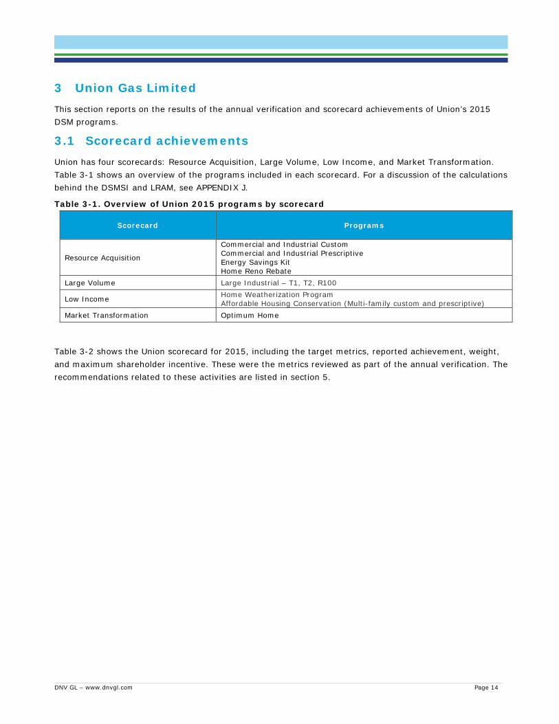
3 Union Gas Limited This section reports on the results of the annual verification and scorecard achievements of Union’s 2015 DSM programs.
3.1 Scorecard achievements Union has four scorecards: Resource Acquisition, Large Volume, Low Income, and Market Transformation. Table 3-1 shows an overview of the programs included in each scorecard. For a discussion of the calculations behind the DSMSI and LRAM, see APPENDIX J.
Table 3-1. Overview of Union 2015 programs by scorecard
Scorecard Programs
Resource Acquisition
Commercial and Industrial Custom Commercial and Industrial Prescriptive Energy Savings Kit Home Reno Rebate
Large Volume Large Industrial – T1, T2, R100
Low Income Home Weatherization Program Affordable Housing Conservation (Multi-family custom and prescriptive)
Market Transformation Optimum Home
Table 3-2 shows the Union scorecard for 2015, including the target metrics, reported achievement, weight, and maximum shareholder incentive. These were the metrics reviewed as part of the annual verification. The recommendations related to these activities are listed in section 5.
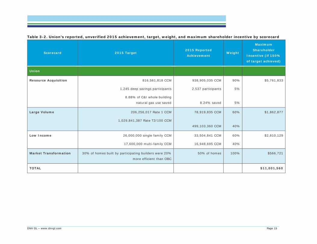
DNV GL – www.dnvgl.com Page 15
Table 3-2. Union’s reported, unverified 2015 achievement, target, weight, and maximum shareholder incentive by scorecard
Scorecard 2015 Target 2015 Reported
Achievement Weight
Maximum
Shareholder
Incentive (if 150%
of target achieved)
Union
Resource Acquisition 816,561,818 CCM
1,245 deep savings participants
8.88% of C&I whole building
natural gas use saved
938,905,035 CCM
2,537 participants
8.24% saved
90%
5%
5%
$5,761,833
Large Volume 206,256,017 Rate 1 CCM
1,029,841,387 Rate T2/100 CCM
78,919,835 CCM
499,103,360 CCM
60%
40%
$1,862,877
Low Income 26,000,000 single family CCM
17,600,000 multi-family CCM
33,504,841 CCM
16,948,695 CCM
60%
40%
$2,810,129
Market Transformation 30% of homes built by participating builders were 20%
more efficient than OBC
50% of homes 100% $566,721
TOTAL $11,001,560

DNV GL – www.dnvgl.com Page 16
3.1.1 Resource Acquisition This section summarizes the results of the EC’s review of the Union Resource Acquisition scorecard. The metrics for the Resource Acquisition scorecard include:
Total cumulative natural gas savings
Number of residential deep savings participants
The average percentage of C&I whole building energy use saved
To verify the natural gas savings, the EC team reviewed each program independently. The programs that contribute energy savings to the Resource Acquisition scorecard are shown in Table 3-3. The table also shows the appendix that has the detailed explanation of the verification activities for each program.
Table 3-3. Union Resource Acquisition programs and report location of detailed verification
Program Location of
Detailed Explanation
Description of Detailed Explanation
Residential Program
Energy Savings Kit APPENDIX E How ESK savings were verified
Home Reno Rebate APPENDIX D How home retrofit program savings were verified
Commercial/Industrial Program
Commercial and Industrial Custom APPENDIX H APPENDIX N
How CPSV / NTG results and spillover are applied for annual verification
Commercial and Industrial Prescriptive APPENDIX C How prescriptive savings were certified
At a high level, the EC completed the following activities to produce verified savings for each Resource Acquisition program:
Energy Savings Kit: The EC reviewed the per-unit savings to ensure that the approved values were used. We then applied adjustment factors from a previously-conducted verification study to produce verified gross savings. Program-assumed free-ridership values were used to produce net savings.
Home Reno Rebate: The EC sampled 25 participants and reviewed the program documentation to confirm that the model savings matched the tracking data. We calculated an adjustment factor and applied it to the tracking savings to produce verified gross savings. Program-assumed free-ridership values were used to produce net savings.
Commercial and Industrial Custom: The EC conducted site verifications as part of the CPSV / NTG study. We also did secondary source research to estimate spillover. We applied the results to produce verified savings for the following sectors:
─ Agriculture and Greenhouse ─ Commercial and Institutional Buildings ─ Industrial
Commercial and Industrial Prescriptive: The EC confirmed energy savings for the population of measures by recreating the program tracking data using program-assumed quantities and approved energy savings per unit to produce verified gross savings. Program-assumed free-ridership values were used to produce net savings.
Table 3-4 shows the gross and net cumulative natural gas savings (CCM), as reported by the utility and verified by the EC. The tables also show the realization rates (RR) of the savings, both in terms of gross

DNV GL – www.dnvgl.com Page 17
savings (those savings which were found to be in place upon the EC’s review) and net savings (those savings which have been adjusted to exclude free riders and include spillover).6 The commercial and industrial custom program has been expanded to more refined sector subsets to match those in the utility-reported tracking data.
Table 3-4. Union’s verified 2015 Resource Acquisition savings
Program
Draft Utility-Reported Savings* Verification Results Verified Savings Gross
Cumulative (m3)
Net Cumulative
(m3)
Gross Realization
Rate†
Net-to-Gross†
Gross Cumulative (m3)
Net Cumulative
(m3) Resource Acquisition
C&I Prescriptive 208,919,006 182,411,887 100% 87% 208,919,006 182,411,887 C&I Custom Ag and Greenhouse 611,477,005 281,279,422 97% 44% 592,368,700 262,534,051
C&I Custom Comm & Inst Buildings
268,582,354 123,547,883 89% 47% 239,199,444 112,642,330
C&I Custom Industrial 593,859,359 273,175,305 103% 43% 612,343,937 260,640,852
Energy Savings Kit 22,398,052 19,567,373 75% 88% 16,882,059 14,800,935
Home Reno Rebate 69,321,370 58,923,165 98% 85% 67,934,943 57,744,701
Total 1,774,557,146 938,905,035 98% 51% 1,737,648,089 890,774,755† * The utility-reported values reflect the savings presented in the utility’s tracking workbook, not in the draft 2015 report. The utility changed the
energy savings values for some projects after submitting the 2015 report but before delivering the data for evaluation, resulting in a small change. †These values are rounded.
To verify the number of residential deep savings participants, the EC followed the process outlined in Table 3-5 and described in APPENDIX D. The EC found 2,529 qualifying deep savings participants compared to 2,537 reported by the program.
Table 3-5. Union deep savings participant verification activities and outcomes
Verification Activity Outcome
Confirm that two major measures were installed for each
sampled site.
Confirmed for 6 of 25 sites using the supplied photos. For
the remaining sites, photos only verified one major
measure.*
Calculate verified cumulative savings for each sampled
site and confirm over 11,000 cumulative m3.
Three of 25 sites did not have cumulative savings over
11,000 cumulative m3 but were identified as deep savings
participants.
Calculate the average percent reduction across the
sample and confirm greater than 25%.
By assuming that the total natural gas consumption was
equal to the space and water heat consumption, we were
able to calculate an average savings reduction of 29%.
Apply the gross realization rate to the population and
determine the number of qualifying deep savings
participants.
The EC found 2,529 qualifying deep savings participants
compared to 2,537 reported by the program.
*Despite the low confirmation rate, the EC did not adjust the outcome based on the initial review. Though the activity did not confirm that there were two major measures, it also did not confirm that there were not. It’s likely that the second major measure was more difficult to visually confirm, such as air sealing.
6 The current spillover estimate is a provisional value based on secondary source research. There is a spillover study in progress. but the results are
not ready.

DNV GL – www.dnvgl.com Page 18
To verify the percentage of whole-building C&I savings, the EC:
Confirmed the calculation method in the Union tracking data
Updated savings based on the CPSV and prescriptive certification
Calculated the verified result.
With the adjustment factors applied, the resulting scorecard metric is 8.08% of whole building energy use saved, as discussed in APPENDIX C.
3.1.2 Large Volume This section summarizes the results of the EC’s review of the Union Large Volume scorecard. The metrics for the Large Volume scorecard are total cumulative natural gas savings by two different rate categories.
To verify natural gas savings, the EC reviewed the prescriptive and custom savings for Large Volume independently. Table 3-6 shows the appendix that has the detailed explanation of the verification activities for each type of project.
Table 3-6. Union Large Volume location of detailed verification
Program Location of Detailed Explanation Description of Detailed Explanation
Large Volume (custom projects) APPENDIX H APPENDIX N
How CPSV / NTG results and spillover are applied for annual verification
Large Volume (prescriptive projects) APPENDIX C How prescriptive savings were certified
At a high level, the EC completed the following verification activities for each Large Volume program:
Custom Projects: The EC conducted site verifications as part of the CPSV / NTG study. We also did secondary source research to estimate spillover. We applied the results to produce verified gross and net savings.
Prescriptive Projects: The EC confirmed energy savings for the population of measures by recreating the program tracking data using program-assumed quantities and approved energy savings per unit to produce verified gross savings. Program-assumed free-ridership values were used to produce net savings.
Table 3-7 shows the gross and net cumulative natural gas savings (CCM), as reported by the utility and verified by the EC. The tables also show the realization rates (RR) of the savings, both in terms of gross savings (those savings which were found to be in place upon the EC’s review) and net savings (those savings which have been adjusted to exclude free riders and include spillover).7 The program has been expanded to more refined rate subsets.
7 The current spillover estimate is a provisional value based on secondary source research. There is a spillover study in progress. but the results are
not ready.

DNV GL – www.dnvgl.com Page 19
Table 3-7. Union’s verified 2015 Large Volume savings
Program
Draft Utility-Reported Savings Verification Results Verified Savings Gross
Cumulative (m3)
Net Cumulative (m3)
Gross Realization
Rate†
Net-to-
Gross†
Gross Cumulative
(m3)
Net Cumulative (m3)
Large Volume
Large Industrial-T1 171,240,007 78,919,835 154% 13% 263,624,641 33,725,518
Large Industrial-T2 1,002,106,837 462,016,235 131% 11% 1,309,850,111 147,448,803
Large Industrial-R100 80,624,184 37,087,125 147% 12% 118,331,969 13,695,699
Total 1,253,971,028 578,023,195 135% 12% 1,691,806,721 194,870,020
† These values are rounded.
3.1.3 Low Income This section summarizes the results of the EC’s review of the Union Low Income scorecard. The metrics for the Low Income scorecard include total cumulative natural gas savings for single family and multi-family participants separately.
To verify energy savings, the EC team reviewed the prescriptive and custom savings for Low Income independently. Table 3-8 shows the appendix that has the detailed explanation of the verification activities for each type of project.
Table 3-8. Union Low Income programs and location of detailed verification
Program Location of
Detailed Explanation
Description of Detailed Explanation
Single Family Program
Home Weatherization Program APPENDIX D How home retrofit program savings were verified
Affordable Housing Conservation Program
Low Income Multi-family (custom projects) APPENDIX H How CPSV / NTG results are applied for annual verification
Low Income Multi-family (prescriptive projects) APPENDIX C How prescriptive savings were certified
At a high level, the EC completed the following verification activities for each Low Income program:
Multi-family Custom Projects: The EC conducted site verifications as part of the CPSV and NTG study and applied the results to produce verified gross and net savings.
Multi-family Prescriptive Projects: The EC confirmed energy savings for the population of measures by recreating the program tracking data using program-assumed quantities and approved energy savings per unit to produce verified gross savings. Program-assumed free-ridership values were used to produce net savings.
Home Weatherization: The EC sampled 25 participants and reviewed the program documentation to confirm that the model savings matched the tracking data. We calculated an adjustment factor and applied it to the tracking savings to produce verified gross savings. Program-assumed free-ridership values were used to produce net savings.
Table 3-9 shows the gross and net cumulative natural gas savings (CCM), as reported by the utility and verified by the EC. The tables also show the realization rates (RR) of the savings, both in terms of gross

DNV GL – www.dnvgl.com Page 20
savings (those savings which were found to be in place upon the EC’s review) and net savings (those savings which have been adjusted to exclude free riders and include spillover).
Table 3-9. Union’s verified 2015 Low Income savings
Program
Draft Utility-Reported Savings* Verification Results Verified Savings Gross
Cumulative (m3)
Net Cumulative
(m3)
Gross Realization
Rate†
Net-to-Gross†
Gross Cumulative
(m3)
Net Cumulative
(m3) Low Income
Low Income Multi-family 17,840,732 16,948,695 96% 95% 17,193,011 16,333,361
Home Weatherization 33,505,239 33,504,841 107% 100% 35,847,824 35,847,426
Total 51,345,970 50,453,536 103% 98% 53,040,835 52,180,787 * The utility-reported values reflect the savings presented in the utility’s tracking workbook, not in the draft 2015 report. The utility changed the
energy savings values for some projects after submitting the 2015 report but before delivering the data for evaluation, resulting in a small change. †These values are rounded.
3.1.4 Market Transformation This section summarizes the results of the EC’s review of the Union Market Transformation scorecard. The metric for the Market Transformation scorecard is the percentage of homes built to Optimum Home standard by participating builders. The Optimum Home standard is greater than 20% above the Ontario Building Code 2012 (OBC). Union reported an achievement of 50.3% of homes built by participating builders, which was confirmed by the EC. The detailed verification efforts are described in APPENDIX I.
3.2 Program spending and cost-effectiveness This section reports on Union’s program spending and cost-effectiveness.
3.2.1 Program spending The Union tracking database included a sheet that reported program spending by scorecard. Table 3-10 shows the Union budget for the portfolio overall. Additional spending detail is in APPENDIX L.
Table 3-10. Union portfolio budget overall
Spending Area OEB-Approved Budget Actual Spending Difference ($) Difference (%)
Programs Sub-total $28,994,667 $29,134,697 $140,030 9%
Research $829,564 $329,116 ($500,448) -57%
Evaluation $1,049,409 $525,012 ($524,397) -46%
Administration $1,713,277 $2,189,940 $476,663 38%
Total DSM Budget $32,588,000 $32,178,766 ($409,234) -7%
3.2.2 Cost-effectiveness Table 3-11 and Table 3-12 show summary results for the TRC, TRC-Plus, and PAC tests, including the cost-benefit ratio and the net present value. Additional detail is shown in APPENDIX M. While there is a general drop in cost-effectiveness results following the verification of savings, almost all OEB-defined programs still pass the cost-effectiveness threshold for all three tests. The only exception is the Home Reno Rebate program, which was not cost-effective when using draft utility reported savings, before any verification-

DNV GL – www.dnvgl.com Page 21
related adjustment.8 When the utility definition of program is used (see APPENDIX M), the threshold is always exceeded.
Table 3-11. Union summary of cost-effectiveness ratio results
Scorecard
Draft using Utility-Reported Savings* Final Verified Ratio
TRC TRC-Plus** PAC** TRC TRC-Plus PAC
Residential Resource Acquisition 1.2 3.0 8.0
1.0 1.2 2.3
Commercial and Industrial Resource Acquisition 2.9 3.3 3.8 12.0
Low Income 1.0 1.1 0.9 1.3 1.4 1.1
Large Volume 4.7 5.4 26.3 6.0 6.9 10.2
Total Portfolio 2.9 3.3 8.1 2.9 3.3 6.8 * The utility-reported values reflect the savings presented in the utility’s tracking workbook, not in the draft 2015 report. The utility changed the
energy savings values for some projects after submitting the 2015 report but before delivering the data for evaluation, resulting in a small change. **These values were calculated using the utility-reported draft savings results. Union only reported TRC in its filings for 2015.
Table 3-12. Union summary of cost-effectiveness net present value results
Scorecard
Draft Net Present Value (M$) using Utility-Reported Savings*
Final Verified Net Present Value (M$)
TRC TRC-Plus** PAC** TRC TRC-Plus PAC
Residential Resource Acquisition 96.7 120.4 117.9
0.4 2.6 6.8
Commercial and Industrial Resource Acquisition 105.4 128.0 124.7
Low Income (0.02) 1.0 (1.1) 1.7 3.1 0.6
Large Volume 70.2 83.6 81.1 27.6 32.6 29.4
Total Portfolio 166.9 205.1 197.9 135.2 166.3 161.5 * The utility-reported values reflect the savings presented in the utility’s tracking workbook, not in the draft 2015 report. The utility changed the
energy savings values for some projects after submitting the 2015 report but before delivering the data for evaluation, resulting in a small change. **These values were calculated using the utility-reported draft savings results. Union only reported TRC in its filings for 2015.
As very low net-to-gross factors were applied to the Large Volume program, the TRC, TRC-Plus, and PAC net values dropped significantly. It is interesting to note that because both savings and costs are affected by the net-to-gross factor, the impact on the TRC and TRC-Plus ratios is far less significant. In addition, a high realization rate (135%) was applied to Union’s Large Volume savings, resulting in an increase of the TRC-Plus ratio, even with a net-to-gross factor of only 12%.
3.3 DSMSI and LRAM This section reports on the results of the DSMSI and LRAM calculations. The recommendations related to these activities are listed in section 5. Table 3-14 shows the verified savings results for the Union portfolio.
8 The Home Reno Rebate program is not required to be cost effective; only the utility-defined Residential program must be cost effective.

DNV GL – www.dnvgl.com Page 22
Table 3-13. Union verified savings results
Program
Draft Utility-Reported Savings* Verification Results Verified Savings Gross
Cumulative (m3)
Net Cumulative
(m3)
Gross Realization
Rate†
Net-to-Gross†
Gross Cumulative
(m3)
Net Cumulative (m3)
Resource Acquisition
Home Reno Rebate 69,321,370 58,923,165 98% 85% 67,934,943 57,744,701
Energy Savings Kit 22,398,052 19,567,373 75% 88% 16,882,059 14,800,935
Total Residential 91,719,422 78,490,538 92% 86% 84,817,002 72,545,636
C&I Custom 1,473,918,718 678,002,610 98% 44% 1,443,912,081 635,817,233
C&I Prescriptive 208,919,006 182,411,887 100% 87% 208,919,006 182,411,887
Total C&I 1,682,837,724 860,414,497 98% 50% 1,652,831,087 818,229,120 Total Resource Acquisition 1,774,557,146 938,905,035 98% 51% 1,737,648,089 890,774,755
Large Volume
Large Volume 1,253,971,028 578,023,195 135% 12% 1,691,806,721 194,870,020
Total Large Volume 1,253,971,028 578,023,195 135% 12% 1,691,806,721 194,870,020
Low Income
Single Family (Part 9) 33,505,239 33,504,841 107% 100% 35,847,824 35,847,426
Multi-family (Part 3) 17,840,732 16,948,695 96% 95% 17,193,011 16,333,361
Total Low Income 51,345,971 50,453,536 103% 98% 53,040,835 52,180,787 * The utility-reported values reflect the savings presented in the utility’s tracking workbook, not in the draft 2015 report. The utility changed the
energy savings values for some projects after submitting the 2015 report but before delivering the data for evaluation, resulting in a small change. †These values are rounded.
3.3.1 DSMSI The EC gathered the verified scorecard achievements from section 3.1 and compared them to the defined upper and lower bands in the Union DSMSI calculation (see APPENDIX J for a description of the DSMSI calculation), shown in Table 3-14. The verified program achievements were entered into the Union tracking workbook DSMSI calculator, which was verified by the EC.

DNV GL – www.dnvgl.com Page 23
Table 3-14. Union’s 2015 scorecard targets, lower band, upper band, and weight
Scorecard Lower Band 2015 Target Upper Band Verified Achievement Weight
Union
Resource Acquisition 612,421,364 CCM
934 participants
7.88%
816,561,818 CCM
1,245 deep savings participants
8.88% of commercial whole building
natural gas use saved
1,020,702,273 CCM
1,556 participants
9.88%
890,774,755 CCM
2,529 participants
8.08%
90%
5%
5%
Large Volume 154,692,013 CCM
772,381,040 CCM
206,256,017 Rate 1 CCM
1,029,841,387 Rate T2/100 CCM
257,820,021 CCM
1,287,301,734 CCM
33,725,518 CCM
161,144,502 CCM
60%
40%
Low Income 19,500,000 CCM
13,200,000 CCM
26,000,000 single family CCM
17,600,000 multi-family CCM
32,500,000 CCM
22,000,000 CCM
35,847,426 CCM
16,333,361 CCM
60%
40%
Market Transformation 25% 30% of homes built by participating
builders were 20% more efficient
than OBC
35% 50.3% 100%

DNV GL – www.dnvgl.com Page 24
The resulting shareholder incentive results are shown in Table 3-15.
Table 3-15. Union DSMSI results Scorecard Draft Utility-Reported DSMSI* DSMSI
Resource Acquisition $4,776,312 $4,010,638
Low Income $2,192,257 $2,462,534
Large Volume $0 $0
Market Transformation $566,721 $566,721
Total $7,535,290 $7,039,894 * Union-reported DSMSI values reflect those presented in Union’s tracking workbook, not in the draft 2015 report. The utility changed the energy
savings values for some projects after submitting the 2015 report but before delivering the data for evaluation, resulting in a small change.
3.3.2 LRAM The EC summed the verified net annual savings by rate class and month. The summed savings were entered into the Union tracking workbook LRAM calculator, which was verified by the EC. Table 3-16 shows the results.
Table 3-16. Union LRAM results
Rate Class Utility-Reported Draft LRAM Verified LRAM
M4 Industrial $77,105 $74,681
M5 Industrial $38,366 $36,890
M7 Industrial $33,512 $32,272
T1 Industrial $2,789 $1,462
T2 Industrial $1,050 $361
20 Industrial $7,002 $6,808
100 Industrial $5,578 $1,894
Total $165,411 $154,368

DNV GL – www.dnvgl.com Page 25
4 Enbridge Gas Distribution, Inc. This section reports on the results of the annual verification and scorecard achievements of Enbridge’s 2015 DSM programs.
4.1 Scorecard achievements Enbridge has five scorecards: Resource Acquisition, Low Income, Residential Savings by Design (RSBD), Commercial Savings by Design (CSBD), and Home Labelling. Table 4-1 shows an overview of the programs included in each scorecard. For a discussion of the calculations behind the DSMSI and LRAM, see APPENDIX J.
Table 4-1. Overview of Enbridge 2015 programs by scorecard
Scorecard Programs
Resource Acquisition
Home Energy Conservation Commercial and Industrial Prescriptive Commercial and Industrial Custom RunitRight
Low Income Low Income Multi-family Low Income Single Family
RSBD RSBD
CSBD CSBD
Home Labelling Home Labelling
Table 4-2 shows the Enbridge scorecard for 2015, including the target metrics, reported achievement, weight, and maximum shareholder incentive. These were the metrics reviewed as part of the annual verification. The recommendations related to these activities are listed in section 5.

DNV GL – www.dnvgl.com Page 26
Table 4-2. Enbridge’s unverified, reported 2015 achievement, target, weight, and maximum shareholder incentive by scorecard
Scorecard 2015 Target 2015 Reported
Achievement Weight
Maximum
Shareholder
Incentive (if 150%
of target achieved)
Enbridge
Resource Acquisition 1,011,900,000 CCM
762 deep savings participants
767,627,826 CCM
5,646 participants
92%
8%
$6,482,744
Low Income 24,100,000 single family CCM
68,700,000 multi-family CCM
40% of Part 3 participants enrolled
28,343,978 CCM
69,226,782 CCM
65% enrolled
50%
45%
5%
$2,495,721
Residential Savings by
Design (Market
Transformation)
18 Builders enrolled
1,111 homes built 20% more efficient than OBC
19 Builders enrolled
1,987 of homes
60%
40%
$1,076,493
Commercial Savings by
Design (Market
Transformation)
18 New developments enrolled 24 developments enrolled 100% $418,269
Home Labelling (Market
Transformation)
5,001 Realtor commitments
4,500 Ratings performed
41,650 Realtor
commitments
333 Ratings performed
50%
50%
$616,397
TOTAL $11,089,624
DNV GL – www.dnvgl.com Page 27
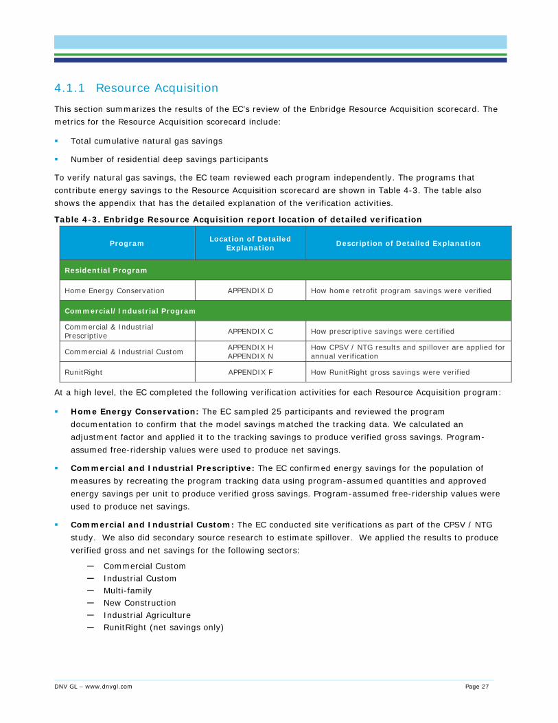
4.1.1 Resource Acquisition This section summarizes the results of the EC’s review of the Enbridge Resource Acquisition scorecard. The metrics for the Resource Acquisition scorecard include:
Total cumulative natural gas savings
Number of residential deep savings participants
To verify natural gas savings, the EC team reviewed each program independently. The programs that contribute energy savings to the Resource Acquisition scorecard are shown in Table 4-3. The table also shows the appendix that has the detailed explanation of the verification activities.
Table 4-3. Enbridge Resource Acquisition report location of detailed verification
Program Location of Detailed Explanation Description of Detailed Explanation
Residential Program
Home Energy Conservation APPENDIX D How home retrofit program savings were verified
Commercial/Industrial Program
Commercial & Industrial Prescriptive APPENDIX C How prescriptive savings were certified
Commercial & Industrial Custom APPENDIX H APPENDIX N
How CPSV / NTG results and spillover are applied for annual verification
RunitRight APPENDIX F How RunitRight gross savings were verified
At a high level, the EC completed the following verification activities for each Resource Acquisition program:
Home Energy Conservation: The EC sampled 25 participants and reviewed the program documentation to confirm that the model savings matched the tracking data. We calculated an adjustment factor and applied it to the tracking savings to produce verified gross savings. Program-assumed free-ridership values were used to produce net savings.
Commercial and Industrial Prescriptive: The EC confirmed energy savings for the population of measures by recreating the program tracking data using program-assumed quantities and approved energy savings per unit to produce verified gross savings. Program-assumed free-ridership values were used to produce net savings.
Commercial and Industrial Custom: The EC conducted site verifications as part of the CPSV / NTG study. We also did secondary source research to estimate spillover. We applied the results to produce verified gross and net savings for the following sectors:
─ Commercial Custom ─ Industrial Custom ─ Multi-family ─ New Construction ─ Industrial Agriculture ─ RunitRight (net savings only)

DNV GL – www.dnvgl.com Page 28
RunitRight: The EC sampled 10 participants to confirm that the calculated energy savings were reasonable. We calculated an adjustment factor and applied it to the tracking savings to produce verified gross savings. The EC applied the results of the NTG study and the secondary source spillover research to produce net savings.
Table 4-4 shows the gross and net cumulative natural gas savings (CCM), as reported by the utility and verified by the EC. The tables also show the realization rates (RR) of the savings, both in terms of gross savings (those savings which were found to be in place upon the EC’s review) and net savings (those savings which have been adjusted to exclude free riders and include spillover).9 The commercial and industrial custom and prescriptive programs have been expanded to more refined sector subsets to match those in the utility-reported tracking data.
Table 4-4. Enbridge’s verified 2015 Resource Acquisition savings
Program
Draft Utility-Reported Savings* Verification Results Verified Savings
Gross Cumulative
(m3)
Net Cumulative
(m3)
Gross Realization
Rate**†
Net-to-
Gross†
Gross Cumulative
(m3)
Net Cumulative (m3)
Resource Acquisition Home Energy Conservation 120,488,487 102,415,214 100% 85% 120,488,487 102,415,214
Prescriptive Commercial 117,938,979 98,693,722 97% 85% 114,897,650 97,416,428
Custom Commercial 210,800,594 185,504,523 91% 21% 192,840,383 40,105,236
RunitRight 2,684,105 2,684,105 100% 53% 2,684,105 1,434,923
Custom Multi-family 152,593,766 122,075,013 91% 38% 139,592,777 53,699,388 C&I Custom New Construction 102,294,475 75,697,912 91% 22% 93,578,986 20,231,777
Custom Industrial 336,500,502 168,250,251 100% 36% 337,417,582 122,387,967 Prescriptive Industrial 10,826,785 7,593,008 100% 70% 10,826,785 7,593,008
Custom Industrial Ag 7,856,800 4,714,080 99% 32% 7,815,133 2,467,184 Total 1,061,984,493 767,627,826 96% 44% 1,020,141,888 447,751,124†
* The utility-reported values reflect the savings presented in the utility’s tracking workbook, not in the draft 2015 report. The utility changed the energy savings values for some projects after submitting the 2015 report but before delivering the data for evaluation, resulting in a small change.
** The gross realization rate for C&I prescriptive includes the removal rate for the multifamily showerhead measure, which was previously included in the net-to-gross adjustment. See APPENDIX C for more detail.
†These values are rounded.
To verify the number of residential deep savings participants, the EC followed the process outlined in Table 4-5 and described in APPENDIX D. The EC found 5,646 qualifying deep savings participants, which is the same number reported by the utility.
9 The current spillover estimate is a provisional value based on secondary source research. There is a spillover study in progress. but the results are
not ready.

DNV GL – www.dnvgl.com Page 29
Table 4-5. Enbridge deep savings participant verification activities and outcomes
Verification Activity Outcome
Confirm that two major measures were installed for each sampled site.
Confirmed for 6 of 24 sites using the supplied photos. For the remaining sites, photos only verified one major measure.*
Calculate the average percent reduction across the sample and confirm greater than 25%.
By assuming that the total natural gas consumption was equal to the space and water heat consumption, we were able to calculate an average savings reduction of 31%.
Calculate the percent reduction for each sample site and compare it to the tracking values.
There were 2 sites with differences; overall, however, the adjusted result was still greater than 25%.
Apply the gross realization rate to the population and determine the number of qualifying deep savings participants.
The EC found 5,646 qualifying deep savings participants, which is the same number reported by the utility.
*Despite the low confirmation rate, the EC did not adjust the outcome based on the initial review. Though the activity did not confirm that there were two major measures, it also did not confirm that there were not. It’s likely that the second major measure was more difficult to visually confirm, such as air sealing.
4.1.2 Low Income This section summarizes the results of the EC’s review of the Enbridge Low Income scorecard. The metrics for the Low Income scorecard include:
Total cumulative natural gas savings for multi-family
Total cumulative natural gas savings for single family
The percentage of Part 3 participants who are also participating in the Low Income Building Performance Management (LIBPM) program
To verify natural gas savings, the EC team reviewed the prescriptive and custom savings for Low Income independently. Table 4-6 shows the appendix that has the detailed explanation of the verification activities for each type of project.
Table 4-6. Enbridge Low Income location of detailed verification
Program Location of
Detailed Explanation
Description of Detailed Explanation
Single Family Program
Low Income Single Family: Winterproofing APPENDIX D How home retrofit program savings were verified
Low Income Single Family non-Winterproofing APPENDIX C How prescriptive savings were certified
Multi-family Program
Low Income Multi-family (prescriptive projects) APPENDIX C How prescriptive savings were certified
Low Income Multi-family (custom projects) APPENDIX H How CPSV / NTG results are applied for annual verification
At a high level, the EC completed the following verification activities for each Low Income program:

DNV GL – www.dnvgl.com Page 30
Multi-family Custom Projects: The EC conducted site verifications as part of the CPSV / NTG study. We applied the results to produce verified gross and net savings.
Winterproofing: The EC sampled 25 participants and reviewed the program documentation to confirm that the model savings matched the tracking data. We calculated an adjustment factor and applied it to the tracking savings to produce verified gross savings. Program-assumed free-ridership values were used to produce net savings.
Single Family and Multi-family Prescriptive Projects: The EC confirmed energy savings for the population of measures by recreating the program tracking data using program-assumed quantities and approved energy savings per unit to produce verified gross savings. Program-assumed free-ridership values were used to produce net savings.
Table 4-7 shows the gross and net cumulative natural gas savings (CCM), as reported by the utility and verified by the EC. The tables also show the realization rates (RR) of the savings, both in terms of gross savings (those savings which were found to be in place upon the EC’s review) and net savings (those savings which have been adjusted to exclude free riders and include spillover).
Table 4-7. Enbridge’s verified 2015 Low Income savings
Program
Draft Utility-Reported Savings Verification Results Verified Savings Gross
Cumulative (m3)
Net Cumulative
(m3)
Gross Realization
Rate**†
Net-to-Gross†
Gross Cumulative
(m3)
Net Cumulative
(m3) Low Income
LI Multi-Family 69,505,240 69,226,782 92% 100% 63,969,354 63,969,354
Single Family 28,410,725 28,343,978 99% 100% 28,067,263 28,067,263
Total 97,915,965 97,570,759 94% 100% 92,036,617 92,036,617 ** The gross realization rate for single family low income and multi-family low income includes the removal rate for some measures, which was
previously included in the net-to-gross adjustment. See APPENDIX C for more detail. †These values are rounded.
To verify the percentage of Part 3 buildings participating in the LIBPM program, the EC:
Confirmed the calculation method
Verified the calculation inputs
Confirmed the overall utility-reported result of 65%.
4.1.3 Residential Savings by Design This section summarizes the results of the EC’s review of the Enbridge RSBD scorecard. The metrics for the RSBD scorecard are the number of builders participating in the RSBD program and the number of houses built to RSBD standard, which is greater than 25% above the Ontario Building Code (OBC) 2012. Enbridge reported achievements of 19 builders enrolled and 1,987 homes built, which was confirmed by the EC. By definition, an enrolled builder must have built a minimum of 50 homes in the previous year to qualify. The detailed verification efforts are described in APPENDIX I.
4.1.4 Commercial Savings by Design This section summarizes the results of the EC’s review of the Enbridge CSBD scorecard. The metric for the CSBD scorecard is the number of developments enrolled in the program. Enbridge reported an achievement

DNV GL – www.dnvgl.com Page 31
of 24 developments enrolled, which was confirmed by the EC. The detailed verification efforts are described in APPENDIX I.
4.1.5 Home Labelling This section summarizes the results of the EC’s review of the Home Labelling scorecard. The scorecard metrics for the Home Labelling scorecard are the number of annual listings by realtors committed to the program and the number of ratings performed. Enbridge reported achievements of 41,650 listings and 333 ratings performed, which were confirmed by the EC.
4.2 Program spending and cost-effectiveness This section reports on Enbridge’s program spending and cost-effectiveness.
4.2.1 Program spending The Enbridge tracking database included reported program spending information. Table 4-8 summarizes the costs across the portfolio. Additional spending detail is in APPENDIX L.
Table 4-8. Enbridge program cost summary
Scorecard/Program OEB-
Approved Budget
Actual Spending Difference
Indirect Direct Total $ %
Program Costs
Resource Acquisition Total $14,443,790 $13,838,372 $3,912,353 $17,750,725 $3,306,935 23%
Residential $1,872,720 $8,340,428 $1,021,867 $9,362,295 $7,489,575 400%
Commercial $8,252,370 $3,923,856 $2,297,867 $6,221,724 ($2,030,646) -25%
Industrial $4,318,700 $1,574,088 $592,619 $2,166,706 ($2,151,994) -50%
Low Income Total $6,864,090 $5,523,356 $1,033,006 $6,556,362 ($307,728) -4% Market Transformation Total $4,890,900 $1,899,739 $1,143,988 $3,043,727 ($1,847,173) -
38% Overhead Total $6,603,160 $0 $7,869,780 $7,869,780 $1,266,620 19%
Resource Acquisition $4,731,485 $0 $5,639,080 $5,639,080 $907,595 19%
Low Income $517,988 $0 $617,349 $617,349 $99,361 19%
Market Transformation $1,353,687 $0 $1,613,352 $1,613,352 $259,665 19%
Incremental Costs $4,920,291 $179 $559,200 $559,378 ($4,360,913) -89%
Total $37,722,231 $21,261,646 $14,518,327 $35,779,973 ($1,942,258) -5%
4.2.2 Cost-effectiveness Table 4-9 and Table 4-10 show summary results for the TRC, TRC-Plus, and PAC tests, including the cost-benefit ratio and the net present value. Additional detail is provided in APPENDIX M. While there is a general drop in cost-effectiveness results following the verification of savings, almost all OEB-defined programs still pass the cost-effectiveness threshold for both the TRC-Plus and the PAC tests. The only exception is the RunitRight program (see APPENDIX M), which was not cost-effective when using utility draft reported

DNV GL – www.dnvgl.com Page 32
savings, before any verification-related adjustment.10 When the utility definition of program is used (see APPENDIX M), the threshold is always exceeded.
Table 4-9. Enbridge summary of cost-effectiveness ratio results
Scorecard Draft using Utility-Reported Savings* Final Verified Ratio
TRC** TRC-Plus PAC TRC TRC-Plus PAC
Resource Acquisition 3.3 3.8 6.0 2.3 2.7 2.7
Low Income 2.1 2.5 2.5 1.6 1.9 1.7
Total Portfolio 3.1 3.6 5.2 2.2 2.5 2.5 * The utility-reported values reflect the savings presented in the utility’s tracking workbook, not in the draft 2015 report. The utility changed the
energy savings values for some projects after submitting the 2015 report but before delivering the data for evaluation, resulting in a small change. **These values were calculated using the utility-reported draft savings results. Enbridge only reported TRC-Plus and PAC in its filings for 2015.
Table 4-10. Enbridge summary of cost-effectiveness net present value results
Scorecard Draft Net Present Value (M$) using
Utility-Reported Savings* Final Verified Net Present Value (M$)
TRC** TRC-Plus PAC TRC TRC-Plus PAC
Resource Acquisition 123.2 149.7 120.4 49.9 61.5 40.7
Low Income 9.2 11.8 10.7 5.0 7.0 5.2
Total Portfolio 132.4 161.6 131.1 54.9 68.5 45.9 * The utility-reported values reflect the savings presented in the utility’s tracking workbook, not in the draft 2015 report. The utility changed the
energy savings values for some projects after submitting the 2015 report but before delivering the data for evaluation, resulting in a small change. **These values were calculated using the utility-reported draft savings results. Enbridge only reported TRC-Plus and PAC in its filings for 2015.
As very low net-to-gross factors were applied to the C&I custom sector, the TRC, TRC-Plus, and PAC net values dropped significantly. It is interesting to note that because both savings and costs are affected by the net-to-gross factor, the impact on the TRC ratio is far less significant.
4.3 DSMSI and LRAM This section reports on the results of the DSMSI and LRAM calculations. The recommendations related to these activities are listed in section 5. Table 4-11 shows the verified savings results for the Enbridge portfolio.
10 The RunitRight program is not required to be cost effective; only the utility-defined Resource Acquisition program must be cost effective.

DNV GL – www.dnvgl.com Page 33
Table 4-11. Enbridge verified savings results
Program
Draft Utility-Reported Savings* Verification Results Verified Savings Gross
Cumulative (m3)
Net Cumulative
(m3)
Gross Realization
Rate**†
Net-to-Gross†
Gross Cumulative
(m3)
Net Cumulative
(m3) Resource Acquisition Home Energy Conservation 120,488,487 102,415,214 100% 85% 120,488,487 102,415,214
Total Residential 120,488,487 102,415,214 100% 85% 120,488,487 102,415,214
C&I Custom 812,730,242 558,925,884 95% 31% 773,928,967 240,326,475
C&I Prescriptive 128,765,764 106,286,730 98% 84% 125,724,435 105,009,436
Total C&I 941,496,006 665,212,614 96% 39% 899,653,401† 345,335,910† Total Resource Acquisition 1,061,984,493 767,627,826 96% 44% 1,020,141,888 447,751,124
Low Income
Single Family (Part 9) 28,410,725 28,343,978 99% 100% 28,067,263 28,067,263
Multi-family (Part 3) 69,505,240 69,226,782 92% 100% 63,969,354 63,969,354
Total Low Income 97,915,965 97,570,759 94% 100% 92,036,617 92,036,617 * The utility-reported values reflect the savings presented in the utility’s tracking workbook, not in the draft 2015 report. The utility changed the
energy savings values for some projects after submitting the 2015 report but before delivering the data for evaluation, resulting in a small change. ** The gross realization rate for C&I prescriptive, single family low income, and multi-family low income includes the removal rate for some measures,
which was previously included in the net-to-gross adjustment. See APPENDIX C for more detail. †These values are rounded.
4.3.1 DSMSI The EC gathered the verified scorecard achievements from section 4.1 and compared them to the defined upper and lower bands in the Enbridge DSMSI calculation (see APPENDIX J for a description of the DSMSI calculation), shown in Table 4-12. The verified program achievements were entered into the Enbridge tracking workbook DSMSI calculator, which was verified by the EC.

DNV GL – www.dnvgl.com Page 34
Table 4-12. Enbridge’s 2015 scorecard targets, lower band, upper band, and weight
Scorecard Lower Band 2015 Target Upper Band Verified Achievement Weight
Enbridge
Resource Acquisition 758,900,000 CCM
571 participants
1,011,900,000 CCM
762 deep savings participants
1,264,900,000 CCM
952 participants
447,751,124 CCM
5,646 participants
92%
8%
Low Income 18,100,000 CCM
51,600,000 CCM
30%
24,100,000 single family CCM
68,700,000 multi-family CCM
40% of Part 3 in LIBPM
30,200,000 CCM
86,000,000 CCM
50%
28,067,263 CCM
63,969,354 CCM
65%
50%
45%
5%
Savings by Design
Residential
13 builders
833 homes
18 builders enrolled
1,111 homes built by participating
builders were 20% more efficient
than OBC
22 builders
1,389 homes
19 builders
1,987 homes
60%
40%
Savings by Design
Commercial
11 developments 18 developments enrolled 24 developments 24 developments 100%
Home Labelling No listings
2,250 ratings
5,001 total listings from committed
realtors
4,500 ratings performed
10,001 listings
6,750 ratings
41,650 listings
333 ratings
50%
50%

DNV GL – www.dnvgl.com Page 35
The resulting shareholder incentive results are shown in Table 4-13.
Table 4-13. Enbridge DSMSI results
Scorecard Utility-Reported Draft DSMSI* Verified DSMSI
Resource Acquisition $6,482,744 $2,612,431
Low Income $1,724,691 $1,483,748
Residential Savings by Design $1,076,493 $1,076,493
Commercial Savings by Design $418,269 $418,269
Home Labelling $616,397 $616,397
Total $10,318,594 $6,207,339
* Enbridge-reported DSMSI values reflect those presented in Enbridge’s tracking workbook, not in the draft 2015 report. The utility changed the energy savings values for some projects after submitting the 2015 report but before delivering the data for evaluation, resulting in a small change.
4.3.2 LRAM The EC summed the verified net annual savings by rate class and month. The summed savings were entered into the Union11 tracking workbook LRAM calculator, which was verified by the EC. Table 4-14 shows the results.
Table 4-14. Enbridge LRAM results
Rate Class Utility-Reported Draft LRAM* Verified LRAM
110 $18,795 $11,769
115 $6,478 $2,932
135 $330 $239
145 $2,267 $876
170 $953 $590
Total $28,822 $16,405
* Enbridge-reported LRAM values reflect those presented in Enbridge’s tracking workbook, not in the draft 2015 report. The utility changed the energy savings values for some projects after submitting the 2015 report but before delivering the data for evaluation, resulting in a small change.
11 The Enbridge tracking workbook calculation did not lend itself to easy update.

DNV GL – www.dnvgl.com Page 36
5 Findings and recommendations This section contains the recommendations from the 2015 annual verification efforts and all other evaluations conducted on the 2015 programs. The annual verification recommendations are in the first section. CPSV / NTG recommendations are in the second section. Some recommendations overlap the various studies and are provided in all sections.
5.1 2015 annual verification recommendations As part of the 2015 annual verification, a number of recommendations were identified. In the tables below, the primary outcomes of the recommendation are classified into three categories: reduce costs (evaluation or program or both), improve savings accuracy, and decrease risk (multiple types of risk are in this category including risk of adjusted savings, risk to budgets or project schedules, and others). Details of the findings, recommendations and outcomes follow the tables.
Table 5-1. Summary of recommendations that apply to the overall annual verification
#
Overall Annual Verification
Recommendation
Applies to Primary Outcome U
nio
n
Enb
rid
ge
Eval
uat
ion
Red
uce
Cos
ts
Imp
rove
Sav
ing
s
Acc
ura
cy
Dec
reas
e
Ris
k
O1A Consider investing in a relational program
tracking database.
O1B Enbridge should include site-level information
for all measures installed through the
program.
O2A Deliver tracking data in a single flat file.
O2B Consider investing in a relational program
tracking database.
O3A Develop and maintain an electronic summary
of the TRM.
O3B Track prescriptive savings using unique
measure descriptions that map to electronic
TRM.

DNV GL – www.dnvgl.com Page 37
Table 5-2. Summary of recommendations that apply to RunitRight
#
RunitRight
Recommendation
Applies to Primary Outcome
Un
ion
Enb
rid
ge
Eval
uat
ion
Red
uce
Cos
ts
Imp
rove
Sav
ing
s
Acc
ura
cy
Dec
reas
e
Ris
k
RR1 Consider adding independent variables to the
regression to account for school breaks.
RR2A Consider including the date when each
activity was implemented.
RR2B Provide information on both the baseline and
installed case.
RR2C Increase the level of documentation when a
single change results in a significant portion
of savings.
RR3A Consider including a basic description of all
end-use equipment served by the gas meter.
RR3B Consider using engineering calculations to
estimate electricity savings.
RR3C Consider reviewing the process for selecting
the HDD reference temperature.

DNV GL – www.dnvgl.com Page 38
Table 5-3. Summary of recommendations that apply to simulation modeling
#
Simulation Modeling
Recommendation
Applies to Primary Outcome
Un
ion
Enb
rid
ge
Eval
uat
ion
Red
uce
Cos
ts
Imp
rove
Sav
ing
s
Acc
ura
cy
Dec
reas
e
Ris
k
SM1 Provide simulation file and output to the
evaluation team.
SM2 Provide more explicit support for major
measure installations.
SM3 Consider reviewing and modifying program
processes to avoid data entry or outdated
simulation result errors.
SM4 Consider funding a study to verify the models
produced by the utility agents.
Table 5-4. Summary of recommendations that apply to cost-effectiveness
#
Cost-effectiveness
Recommendation
Applies to Primary Outcome
Un
ion
Enb
rid
ge
Eval
uat
ion
Red
uce
Cos
ts
Imp
rove
Sav
ing
s
Acc
ura
cy
Dec
reas
e
Ris
k
CE1 Allocate “sector”-level administrative costs
and overhead to each individual program and
report program-level cost-effectiveness
results.
CE2 Use a consistent real discount rate of 4%
when using real streams of benefits and
costs.
CE3 Explore the possibility of better defining water
avoided costs.
CE4 Work towards better uniformity in methods
and assumptions.

DNV GL – www.dnvgl.com Page 39
Table 5-5. Summary of recommendations that apply to other areas
#
Other
Recommendation
Applies to Primary Outcome
Un
ion
Enb
rid
ge
Eval
uat
ion
Red
uce
Cos
ts
Imp
rove
Sav
ing
s
Acc
ura
cy
Dec
reas
e
Ris
k
OR1 When the C&I deep savings metric is used,
deliver monthly billing data for each C&I
participant.
OR2 Provide a detailed explanation for the DSMSI
calculation.
5.1.1 Overall annual verification recommendations O1. Finding: The Enbridge tracking database does not currently include information that allows the
evaluator to identify all the projects installed by a single customer. Without this information, the EC could not identify projects installed across customers to determine whether interactive effects may have reduced energy savings. Some prescriptive measures in the Enbridge data did not have site-level information at all, only a summary of the energy savings for that technology across all sites.
Recommendation A: Both utilities should strongly consider investing in relational program tracking databases. Relational program tracking databases and customer relationship management (CRM) systems allow for multiple measures and projects to be associated with a single customer and/or customer site. The incremental cost of implementation is low if it is part of the initial database design, populated as projects are started, and updated once they are complete.
Outcome: Reduced burden on utility staff and reduced evaluation costs. A relational database would streamline aggregation of program data for scorecards and make providing data simpler for annual savings evaluation and verification.
Recommendation B: Enbridge should include site-level information for every measure installed in the program.
Outcome: Confirmation that each installation is unique.
O2. Finding: Both utilities invested significant effort in developing Excel-based tracking workbooks that summarized data and calculated DSMSI based on utility-reported results. Union’s workbook included a feature that was designed to allow evaluators to enter adjustment factors in a single location and automatically update DSMSI and LRAM calculations. Neither workbook was well suited for evaluation efforts.

DNV GL – www.dnvgl.com Page 40
Recommendation A: Deliver to evaluators a single, flat file of tracking data.12 Each record should have measure-level information which includes the information listed below.
Program identification information, such as scorecard, and program name
Customer identification information, such as a unique customer ID, rate class, and location
Measure identification information, such as measure description, unique measure identification, measure group, measure life, free rider rate, and savings per unit for prescriptive measures
Savings information, such as annual gross and net savings, cumulative gross and net savings, and non-gas savings
Additional information as needed to allow the evaluator to verify LRAM and cost-effectiveness
The Union tracking data most closely followed this recommendation, but both utilities invested in workbook features that did not enhance evaluation efficiency.
Outcome: Reduced burden on program staff, more flexibility for evaluators.
Recommendation B: See recommendation O1A. The utilities should consider investing in a new database.
Outcome: Reduced burden on utility staff and reduced evaluation costs.
O3. Finding: Neither Union nor Enbridge tracking databases currently use prescriptive measure descriptions that map directly to the approved energy savings spreadsheet (TRM). The EC often struggled to align tracking measures to the correct TRM measure, which resulted in repeated back-and-forth between evaluation and the utilities for clarification. During this process, the EC found that some Enbridge measures were assigned to the wrong sub-category by capacity or other size measure. The EC also found that some Enbridge measures were assigned outdated savings values from previously-approved TRMs.
Recommendation A: Develop and maintain an electronic summary of the TRM, such as an Excel file. Each measure (identified as a unique savings value) should have an assigned measure ID number, and new ID numbers should be assigned when a measure is updated with a new savings value. This allows for a historical record of the changes in the TRM and allows the evaluation to identify outdated values.
Recommendation B: Track prescriptive savings using unique measure descriptions that clearly map to the electronic TRM.
Outcome: Reduced burden on utility staff and reduced evaluation costs. Fewer errors in the tracking data.
5.1.2 RunitRight savings recommendations RR1. Finding: Not all the RunitRight regression models provided a strong fit for the consumption data. In
particular, school buildings, which have widely inconsistent occupancy throughout the year, show low R-squared values.
12 In this context, a flat file is a table with one record per line and no summary information.

DNV GL – www.dnvgl.com Page 41
Recommendation: Consider including additional independent variables for schools to account for break periods, which may improve the regression fit.
Outcome: More confidence in the reported savings estimates.
RR2. Finding: The RunitRight documentation includes a description of the activities at each site, which are documented in the calculation workbook and annual site report. The same level of documentation is included for all activities, regardless of the percentage of savings contributed by that activity.
Recommendation A: Consider including the date when each activity was implemented.
Recommendation B: Provide information on both the baseline and installed case. For example, when a schedule is reset, provide the pre- and post-installation schedule.
Recommendation C: Increase the level of documentation on end use equipment when a change to that equipment results in a significant reduction in consumption.
Outcome: More confidence in the reported savings estimates.
RR3. Finding: The evaluator observed a number of opportunities to improve the savings estimates associated with the RunitRight program, including savings at the electric meter. Some sites had base loads that were unexpectedly sensitive to the reference temperature.
Recommendation A: Consider including a basic description of the end-use equipment served by the gas meter, such as DHW, heating, or cooking. This will help the reviewer better assess the consumption patterns occurring over time and the magnitude of base load and weather-sensitive savings estimated.
Recommendation B: Consider using engineering calculations to estimate electric energy savings to capture the full value of the program.
Recommendation C: Consider reviewing the process for selecting the HDD reference temperature to reduce baseload sensitivity.
Outcome: More accurate savings estimates.
5.1.3 Simulation modeling recommendations SM1. Finding: Both utilities use building simulation modeling to estimate energy savings for their home
retrofit programs, including Home Energy Conservation, Home Reno Rebate, Winterproofing, and the Home Weatherization Program. HOT2000 is the most common program used for those simulations, which is a program developed and released by NRCan for certified energy advisors. Because of the restrictions on the program, the evaluator could not consistently run the simulation files and produce the same result reported by the program.
Recommendation: Provide both the building simulation file and the program output to the evaluation team. By delivering both, the evaluation team would not have to follow up with the utility to obtain output for models that could not be run, but could still verify the output for models that can be run.
Outcome: Reduced burden on utility staff and reduced evaluation costs.
SM2. Finding: Both utilities have market-rate scorecard metrics that rely on a definition of deep savings that is related to the number of “major” measures installed at a site. Both utilities also collect and deliver photographs to support many of the changes made at a home retrofit site. However, the

DNV GL – www.dnvgl.com Page 42
evaluator could not consistently confirm the number or type of major measures installed based on the photographs or other documentation provided.
Recommendation: Consider providing more explicit support for each major measure to eliminate uncertainty around the number of deep savings program participants.
Outcome: Greater certainty around scorecard achievements.
SM3. Finding: The evaluator identified a number of inaccurate savings entries due to data entry errors or outdated Union home retrofit simulation results. Many of these errors could be avoided through changes in program processes.
Recommendation: Consider reviewing and modifying program processes to avoid similar errors in the future.
Outcome: Reduced burden on utility staff and reduced evaluation costs.
SM4. Finding: The energy savings from the home retrofit programs rely exclusively on the simulations provided by the delivery agents. Those simulations likely rely on a number of assumptions or standard modeling practices which may or may not follow industry standards. A detailed review of the models was outside the scope of the annual audit.
Recommendation: Consider funding a study to verify the models produced by the utility agents to ensure they conform to standard industry practice.
Outcome: Greater certainty around savings estimates.
5.1.4 Cost-effectiveness recommendations CE1. Finding: In some cases, the Union program costs were grouped together for several programs. To
get program- or sector-level cost-effectiveness results, the EC prorated costs to programs based on natural gas savings.
Recommendation: Allocate “sector”-level administrative costs and overhead to each individual program and report program-level cost-effectiveness results.
Outcome: Greater certainty around program-level achievements.
CE2. Finding: Enbridge uses a real discount rate of 4% and applies it to streams of current (nominal) values. However, the real discount rate should only be applied to real (inflation-adjusted) streams of benefits and costs. Nominal discount rates should be applied to streams of current (nominal) values.
Recommendation: Use a consistent real discount rate of 4% for both Enbridge and Union when using “real” (inflation-adjusted) streams of benefits and costs.
Outcome: More accurate cost-effectiveness results.
CE3. Finding: Water rates are currently used as a proxy for the water avoided costs. Water avoided costs should only include the marginal impact from reduced consumption. Using the full rate as the avoided cost may be appropriate in some jurisdictions with a completely variable rate structure. However, those with high fixed costs (which, in our experience, can represent 75% to 80% of water costs) should use a true avoided cost.

DNV GL – www.dnvgl.com Page 43
Recommendation: Explore the possibility of better defining water avoided costs.
Outcome: More accurate cost-effectiveness results.
CE4. Finding: The EC found major discrepancies in the way the utilities calculate cost-effectiveness. Some areas of discrepancies included the discount rate, the use of a non-energy benefit adder, the format of reporting results, and the allocation of administration and overhead costs by program. While there is always a balance to be found between uniform methods and the need to account for each specific utility’s needs, greater uniformity could be achieved.
Recommendation: Work towards a better uniformity of cost-effectiveness methods and assumptions between the two gas utilities.
Outcome: More accurate and consistent cost-effectiveness results.
5.1.5 Other recommendations OR1. Finding: The Union scorecard includes a metric that relies on an understanding of the whole-
building energy use for each C&I program participant. The program data included the total annual consumption at each site, normalized by a regional (north or south) estimate of heating degree days. The calculation appeared to assume that industrial sites were not weather-sensitive but commercial sites were.
Recommendation: When the C&I deep savings metric is used, deliver monthly billing data for each C&I participant to allow the EC to verify the annual consumption values and the weather sensitivity assumptions. Provide the supporting information (and calculation, if possible) for the normalized regional heating degree days.
Outcome: Greater certainty around scorecard achievements.
OR2. Finding: The evaluator was unable to locate a source document that supports the utilities’ calculation of DSMSI. Given the importance of the shareholder incentive, it is appropriate to have a clearly defined and detailed explanation of how it is calculated.
Recommendation: Provide a detailed explanation for the DSMSI calculation for review by the EC and OEB.
Outcome: Greater certainty around shareholder incentives.
5.2 CPSV / NTG findings and recommendations As part of the CPSV / NTG evaluations, a number of recommendations were identified. In the tables below, the primary outcomes of the recommendation are classified into four categories: reduce costs, increase savings, increase (or maintain) customer satisfaction and decrease risk (multiple types of risk are in this category including risk of adjusted savings, risk to budgets or project schedules, and others). Details of the findings, recommendations and outcomes follow the tables.

DNV GL – www.dnvgl.com Page 44
Table 5-6: Energy savings and program performance recommendations
#
Energy Savings and Program
Performance
Recommendation
Applies to Primary Outcome
Un
ion
Enb
rid
ge
Eval
uat
ion
Red
uce
Cos
ts
Incr
ease
Sav
ing
s
Incr
ease
Cu
sto
mer
Sat
isfa
ctio
n
Dec
reas
e
Ris
k
ES1 The utilities should continue in their
commitment to accuracy.
ES2 Evaluate free-ridership for the programs
annually and couple the free-ridership
evaluation with process evaluation
ES3 Error ratios from this report inform sample
design for future evaluation.
ES4 Align the program design with cumulative net
goals
ES5 Do not pay incentives until after installation is
complete.
ES6 Develop policies to collaborate across electric
and gas projects to avoid double-counting fuel
savings and increases from energy efficiency
measures.
ES7 Consider establishing a policy to define rules
around energy savings calculation for fuel
switching and district heating/cooling
measures.
ES8 Consider establishing a policy that defines an
eligibility floor and cap based on simple
payback period for energy efficiency projects.
ES9 Consider establishing an official definition for
EUL and implementing a study to define EULs
for program measures
ES10 Track metrics for how long it takes from the
final installation verification to the posting of
incentive payments.

DNV GL – www.dnvgl.com Page 45
#
Energy Savings and Program
Performance
Recommendation
Applies to Primary Outcome
Un
ion
Enb
rid
ge
Eval
uat
ion
Red
uce
Cos
ts
Incr
ease
Sav
ing
s
Incr
ease
Cu
sto
mer
Sat
isfa
ctio
n
Dec
reas
e
Ris
k
ES11 Increase transparency of “influence
adjustments” and do not include in gross
savings
ES12 Conduct a process evaluation to improve
Large Volume influence on customer projects
ES13 Consider approaches to market that leverage
third-party vendors.
Table 5-7: Verification process recommendations
#
Verification Process
Recommendation
Applies to Primary Outcome
Un
ion
Enb
rid
ge
Eval
uat
ion
Red
uce
Cos
ts
Incr
ease
Sav
ing
s
Incr
ease
Cu
sto
mer
Sat
isfa
ctio
n
Dec
reas
e
Ris
k
VP1 Modify contracts to require participants to
agree to comply with EM&V as well as utility
representatives as part of the requirements
for participation in the program.
VP2 The verification and utility staff should agree
to a code of conduct for each role during
onsite visits.

DNV GL – www.dnvgl.com Page 46
Table 5-8: Documentation and Support recommendations
#
Documentation and Support
Recommendation
Applies to Primary Outcome
Un
ion
Enb
rid
ge
Eval
uat
ion
Red
uce
Cos
ts
Incr
ease
Sav
ing
s
Incr
ease
Cu
sto
mer
Sat
isfa
ctio
n
Dec
reas
e
Ris
k
DS1 Take steps to improve documentation:
Include explicit sources for all inputs and assumptions in the project documentation.
Store background studies and information sources with the project files and make them available to evaluators.
Provide evaluators full access to customer data.
Provide pre- and post-installation photos, where available.
Document and provide internal M&V documents where available.
Institute a checklist as part of project closeout to ensure all relevant project documentation is assembled as ready for verification
DS2 Ensure that incremental costs are supported
by invoices or other documentation
DS3 Increase the amount of documentation and
source material for projects that have greater
energy savings.
DS4
A
Digitize and file project documentation for all
projects as they are completed and paid
during project closeout.
DS4
B
Until the utilities can implement an effective
digital document storage process, the
evaluation should allow more time for the
utilities to assemble and deliver the
documentation.
DS5 Consider providing more training or adding
quality control steps to ensure the summary
workbook front page is completed and stored
in a consistent manner.
DS6 Use a consistent summary workbook.

DNV GL – www.dnvgl.com Page 47
Table 5-9: Data management recommendations
#
Data Management
Recommendation
Applies to Primary Outcome
Un
ion
Enb
rid
ge
Eval
uat
ion
Red
uce
Cos
ts
Incr
ease
Sav
ing
s
Incr
ease
Cu
sto
mer
Sat
isfa
ctio
n
Dec
reas
e
Ris
k
DM1
A
Track contacts associated with projects in the
program tracking database.
DM1
B
Strongly consider investing in relational
program tracking databases.
DM1
C
Include structure for improved data integrity
in the evaluator request for contact
information for the 2016 and 2017 savings
verification and evaluation.
DM2
A
Consider offering bonus incentives early in the
year to combat the “hockey stick”
phenomenon where a large percent of
projects get closed in the fourth quarter of the
year (which results in rushed QC for data).
DM3 Track and provide to evaluators dates for key
milestones in the project.
DM4 Maintain a customer identifier in the database
to clearly identify related sites.
DM5 Include EUL (also remaining useful life for
dual baselines), NTG, and each of the key
savings types (i.e., annual and cumulative,
gross and net) in the program tracking
extracts provided to evaluators.
Figure 5-1 shows an approximate cost vs. impact relation ship for each of the recommendations on a 4-point scale. The upper left quadrant of the figure shows the recommendations that are relatively low cost that would have a high impact. Those in the upper right are recommendations where both cost and impact are high.

DNV GL – www.dnvgl.com Page 48
Figure 5-1: Approximate Cost vs. Impact of each recommendation
5.2.1 Energy savings and program performance ES1. Finding: Both utilities exhibit a strong commitment to accurate energy savings estimates. Both
utilities have made significant investments in developing calculation tools which model savings accurately. For example, Union’s dock door seal calculator is well considered and designed, and Enbridge’s Etools calculator is very thorough in attempting to model savings for key measures.
Both utilities chose to retain engineers with strong understandings of their customers’ building and process systems. We had numerous opportunities to interact with these engineers on phone calls and site visits, and have grown to respect their knowledge and engagement with the types of systems that matter to their customers.
Both utilities showed a commitment to finding accurate savings. On several occasions, both on the phone and in writing, the evaluation team suggested a value that would have increased savings in a way that the program engineer did not think was valid. When this happened, neither utility was shy in suggesting that we may want to make a more conservative choice.
Recommendation: The utilities should continue in their commitment to accuracy.
Outcome: Accurate energy savings.
ES2. Finding: Free-ridership in the utilities’ programs is high
Recommendation: With high free-ridership and rapidly changing programs, consistent evaluation of free-ridership annually and free-ridership evaluation coupled with process evaluation will help identify specific ways for each program to manage and reduce free-ridership.

DNV GL – www.dnvgl.com Page 49
Outcome: Effective free-ridership management will allow the programs to increase their net savings significantly in future years.
ES3. Finding: Relative precision targets were exceeded for some programs and not met for others.
Recommendation: Error ratios from the results provided in this report should be used to inform sample design for future evaluation years.
Outcome: Better defined error ratios for the measures in the programs will allow more efficient sample design for future evaluations, improving precisions and reducing costs.
ES4. Finding: Attribution for the programs came primarily through acceleration rather than changes in efficiency or quantity/size. This is partly due to the measures that dominate the programs: controls, maintenance, and optimisation. These measures do not have varying efficiencies, so the programs are either affecting the number of units implemented or accelerating the measure. Acceleration is less valuable to programs that are seeking to meet cumulative net goals. Acceleration periods tend to be considerably shorter than the estimated useful life (EUL) of a measure and thus the partial attribution that results is low relative to cumulative gross savings.
Recommendation: To align the programs with cumulative net goals, the utilities should seek to:
continue promoting long life measures and consider discontinuing promotion of short lived measures proactively upsell equipment purchases from standard to efficient products target hard to reach customers who have not participated in the past promote EE measures with low market penetration (such as heat reflector panels) motivate customers to increase the scope of their projects, some options include multi-measure
bonuses or escalating incentive structures that pay more for doing more
Outcome 1: Focusing on proactive sales rather than reactive will help the net-to-gross (NTG) ratio.
Outcome 2: Effective free-ridership management will allow the program to increase net savings significantly in future years.
ES5. Finding: A handful (<5) of respondents indicated that all or part of their incentivized project had not yet been installed over a year after the incentive was paid.
Recommendation: Do not pay incentives until after installation is complete.
Outcome: Cost-effectiveness of the program will increase as it avoids paying for savings that do not materialize.
ES6. Finding: Some customers receive incentives from their electric provider and natural gas utility to complete the same EE measure. Both providers may claim the same changes in energy use, resulting in overlap when aggregated across fuels at the provincial level.
Recommendation: Develop policies to collaborate across electric and gas projects to avoid double-counting fuel savings and increases from energy efficiency measures.
Outcome: More accurate energy and carbon savings estimates across the province.
ES7. Finding: Some measures (e.g., geothermal heat pumps, combined heat and power, and those that save district heating energy) have difficult-to-define baseline technologies.
DNV GL – www.dnvgl.com Page 50
Recommendation: Consider establishing a policy to define rules around energy savings calculation for fuel switching and district heating/cooling measures.
Outcome: Less evaluation risk and a better alignment between province energy efficiency goals and program implementation.
ES8. Finding: Projects with very long and very short simple payback periods often have low NTG ratios. However, from a customer service standpoint, it may be difficult for utilities to deny incentives to customers unless they have pre-established rules to point to.
Recommendation: Consider establishing a policy that defines an eligibility floor and cap based on simple payback period for energy efficiency projects.
Outcome: The rule will give utilities a guideline to restrict the program to projects that are more likely to result in net savings. It will also allow the utilities to reject potentially poor projects without a large effect on customer satisfaction.
ES9. Finding: Members of the EAC and evaluation team have different understandings of the definition of some evaluation inputs.
Recommendation: Consider establishing an official definition for EUL and implementing a study to define EUL for all measures, especially steam traps, pipe leaks, steam leaks, condensate leaks, and pipe insulation.
Outcome: The study will improve the accuracy of lifetime savings estimates.
ES10. Finding: A handful (<5) of sites reported unhappiness with delays in receiving their incentive payment (5 months).
Recommendation: Track metrics for how long it takes from the final installation verification to the posting of incentive payments. Consider holding program managers accountable to these metrics by considering them during performance reviews, building in performance bonuses if all payments are posted within one month, and/or implementing a penalty if it takes greater than three months to post any payments.
Outcome: Improved customer satisfaction.
ES11. Finding: Influence adjustments were made to projects that adjusted the gross savings for “net” or program influence reasons. Accounting of which projects had these adjustments was not maintained by the program and the adjustments were included in different places in project calculation workbooks, making their identification challenging. In addition, the program NTG was also applied to these projects, effectively double discounting savings in scorecards.
Recommendation: If the utility chooses to continue making influence adjustments to the savings upon which it calculates savings, these adjustments should be made more transparent and not included in the reported gross savings for the program in scorecards. Instead the specific project influence adjustment should be included in the scorecard in place of the general program or domain level NTG factor.
Outcome: Reduced risk of double adjustments.
ES12. Finding: Union’s Large Volume program has a very high amount of free-ridership.

DNV GL – www.dnvgl.com Page 51
Recommendation: This evaluation did not include a process evaluation. Union should consider conducting a process evaluation focused on how to reduce the rate of free-ridership. Three options that the Union might consider are:
Eliminate measure types with high free-ridership (Union indicated that most maintenance type measures were eliminated in 2016).
Use an application process that includes a committee review that can reject free riders. This option is hard for utilities to manage as it can affect customer satisfaction negatively
Clear payback criteria such as initial payback must be longer that X years and the incentive paid must reduce payback below Y years. This has the advantage of being a rule that account representatives can explain when talking to customers.
Non-energy benefits of projects that large industrial customers gravitate to are often large compared to energy saving benefits, so simple payback criteria will not eliminate all free rider projects. Awareness of this issue should be promoted among the implementation team.
Outcome: Effective free-ridership management may allow the program to increase its net savings significantly in future years.
ES13. Finding: Vendor attribution did not increase overall program attribution significantly. Of the vendors that customers cited as influences, few indicated that either program had much effect on the projects.
Recommendation: The utilities should consider approaches to market that leverage third-party vendors. A process evaluation that includes vendor interviews might uncover opportunities.
Outcome: Effective leveraging of vendors could both increase NTG ratios and increase program uptake.
5.2.2 Verification processes VP1. Finding: DNV GL was unable to obtain access to all the equipment at all the sites selected for
verification. Both Enbridge and Union have several large projects with industrial companies, including food processing, refineries, and other industries. In many cases, the customer refused to provide SCADA data or similar trend data to allow a reasonable verification of the project. This means we were unable to do more than a reasonableness check on the savings.
A review of the Enbridge contract shows that the customer is not required to provide the information that is necessary for EM&V. The most relevant sections are:
Item 6 states: Payment of the Incentive Payment is subject to the completion of a satisfactory site inspection of the improvements, including the installed equipment by an authorized representative of Enbridge.
Item 9 states: Upon request within eighteen months of the commissioning date of the Project, and with reasonable notice, the Customer agrees to provide authorized representatives of Enbridge with access to the Project, and with required information or data relating to the project for the purposes of the Application and these General Terms and Conditions.
Neither of these are sufficient for EM&V.
Recommendation: Modify contracts to require participants to agree to comply with EM&V as well as utility representatives as part of the requirements for participation in the program.

DNV GL – www.dnvgl.com Page 52
Outcome: Reduced evaluation costs and risks. Participant non-compliance requires evaluators to request documentation for a large backup sample, and to survey and/or visit additional sites to obtain sufficient data for the evaluation. The process of contacting a site and getting a refusal costs time and money, as does the substitution of an additional site to make up for the unobtained data. In some cases, there might not be additional sites to sample, in which case the evaluation estimates will have lower precision than they would with full compliance.
VP2. Finding: Verification engineers and verification forms caused confusion with site contacts and the length of visits also led to a handful of customer complaints. Utility staff at a handful of sites responded to questions in place of participating customers and in one case interfered with data collection.
Recommendation: The verification and utility staff should agree to a code of conduct for each role. The teams should receive clear direction as to the dos and don’ts of all parties involved in site visits, including both verification engineers and utility staff should they attend the visit. Open lines of communication between the site team and utility staff should be maintained to reduce misunderstandings and ensure that the teams are on the same page as to each other’s role.
In general, the following should be part of standard verification practices:
Ensure site engineer reviews final site report for accuracy post-audit. Align data collection forms with site report structure to reduce communication and transcription
errors. Ensure data appropriate to determining EUL is collected while on-site (i.e., make EUL
determination a primary, rather than secondary focus). Request specific documentation or data from systems prior to site visit (allowing for adequate
time for site contact to obtain).
Outcome: Improved data collection and customer satisfaction.
5.2.3 Documentation and support DS1. Finding: Project documentation for some projects lacked sufficient details to allow evaluators to
reproduce the calculations made by program staff or third-party vendors. Specific issues included:
Project data or details missing Insufficient measure-level details to fully describe what was installed Descriptions that were difficult to understand Use of black box tools Hardcoded information in calculation spreadsheets Energy intensity changes presented without providing the data to justify it Undocumented assumptions Sources referenced but not included or available, such as feasibility studies and historical
analysis of energy use that was left out of the project documentation Scanned documents that were unreadable Input adjustments that approximate other effects, but are not explained Insufficient access to customer data (by customers) for confidentiality reasons. Modelling files that could not be opened Adjustments to savings estimates for safety or influence that were not clearly marked, sourced,
or carried out in a consistent fashion

DNV GL – www.dnvgl.com Page 53
Etools files not provided for many industrial boiler & boiler add-on projects
Recommendation: Several steps could be taken to improve data quality:
Include explicit sources for all inputs and assumptions in the project documentation. Store background studies and information sources with the project files and make them available to
evaluators. Provide evaluators full access to customer data. Provide pre- and post-installation photos, where available. Document and provide internal M&V documents where available. Institute a checklist as part of project closeout to ensure all relevant project documentation is
assembled as ready for verification
Outcome: Properly explaining and sourcing the savings calculation method and assumptions allows the evaluating engineer to more easily identify what needs to be verified. It also makes it easier to determine whether the methods and assumptions are reasonable and use ex ante assumptions rather than seek documented values elsewhere.
DS2. Finding: Invoices were not always included with documentation, and we saw a handful (<5) of cases where utility program staff were overclaiming incremental costs. This did not appear to be systemic, but higher incremental costs enable payment of a larger incentive.
Recommendation: Ensure that incremental costs are supported by invoices or other documentation, especially for add-on and optimization measures where the total cost and incremental cost are likely to be the same. Equipment replacement measures may require an additional standard efficiency quote to produce incremental cost.
Outcome: Incremental cost is an important component of simple payback, which is often used to judge the economic benefit of energy efficiency projects. It is also an input to some benefit-cost tests.
DS3. Finding: Larger projects appeared to fall under the same documentation standards as smaller projects.
Recommendation: Increase the amount of documentation and source material for projects that have greater energy savings.
Outcome: Projects that are better documented tend to have more accurate savings estimates and receive fewer evaluation adjustments than those that are less documented. Large projects have a greater effect on overall savings adjustment factors. Therefore, large projects with better documentation are more likely to result in adjustment factors closer to 100%.
DS4. Finding: Enbridge did not maintain complete digital project files prior to the evaluation request. Union appeared to have digital documentation that was not completely assembled prior to evaluation.
Recommendation A: Digitize and file project documentation for all projects as they are completed and paid during project closeout. PDF and Excel files associated with a project should be stored in a way that allows them to be easily found and associated with a specific project and/or customer. The best practice is to include a document repository as part of the program tracking system with a separate folder for each project.

DNV GL – www.dnvgl.com Page 54
Recommendation B: Until the utilities can implement an effective digital document storage process, the evaluation should allow more time for the utilities to assemble and deliver the documentation.
Outcome: In our experience, DSM programs that store complete and well-organized digital records experience less evaluation risk. In other words, their gross savings adjustments are closer to 100%. This happens for three reasons:
Digitization facilitates internal review of project documentation, providing additional opportunities to identify missing information and errors
Assembly during project closeout improves the comprehensiveness of the documentation because less time has elapsed than if it was assembled for evaluation, so less information is lost or forgotten
Easy retrieval makes it more likely that the complete file is sent to the evaluation team, reducing the information gap between implementation and evaluation.
DS5. Finding: Union custom projects utilized a project application summary workbook that summarizes the key project inputs, calculations, and most details. In general, this is a good approach that facilitates internal review and evaluation. One challenge was that different projects used the workbook in different ways:
The notes section was sometimes used to identify and highlight specific unique approaches and features in projects, but not always.
Calculations internal to the summary page were consistent for most projects, but not all (additional factors were sometimes added).
Sub-methods critical to the calculation were contained in hidden sheets. Safety and influence adjustments were inserted in different locations and not always explained.
Recommendation: Consider providing more training or adding quality control steps to ensure the summary workbook front page is completed and stored in a consistent manner. Identify a common approach for common measures and, if necessary, document deviations and the reasons for the deviations in a clearly labelled field on the summary sheet.
Outcome: A consistent summary workbook aids both internal and external quality assurance, quality control, and measurement and verification.
DS6. Finding: The Enbridge Etools is used as both a calculation tool and as a communication tool with customers. While it appears to serve the needs of the program, this form of communication is difficult for the evaluation efforts.
Etools does not easily allow for assumptions to be sourced within the record. Some Etools selections may be site-specific and some may be defaults; the calculator does not
distinguish. Energy savings that are calculated outside of Etools are hard-entered in Etools but not always
sourced.
Recommendation: Use a consistent summary workbook.
Outcome: A consistent summary workbook aids both internal and external quality assurance, quality control, and measurement and verification.

DNV GL – www.dnvgl.com Page 55
5.2.4 Data management DM1. Finding: Neither Union nor Enbridge currently track participating customer or participating vendor
contact information in their program tracking database. Providing the information to the evaluation put significant burden on utility staff. When contact information was provided, there were significant data integrity issues including contacts listed in the wrong places, partial addresses, and incorrect or missing phone numbers and email addresses.
Recommendation A: Track contacts associated with projects in the program tracking database. At a minimum, the program tracking database should include:
Project site address Customer mailing address Primary customer contact name Primary customer contact phone Primary customer contact email Primary customer contact mailing address
Addresses are best tracked as multiple fields including:
o Street address line 1 o Street address line 2 o City o Province o Postal code
Phone number fields should include data validation to enforce a consistent format and avoid missing or extra digit errors. Phone extensions should be tracked in a field separate from the ten-digit phone number and be restricted to numeric data only.
The best practice is to maintain contacts in a table separate from specific project or customer data. This allows for a single contact to be connected to multiple accounts and/or projects as necessary without creating duplication. This structure also makes it easier to associate multiple contacts with a single project.
Vendor contact information should also be tracked in the database, in the same table as the participating customer contact information. With a relational database, the contact ID from the table can be added to a project record in the role consistent with the contact’s participation (such as vendor, decision maker, or technical expert) with a separate table that allows a single vendor contact to be associated with multiple projects.
Outcome A: Reduced burden on utility staff to seek contact information for projects, whether for internal or evaluation use. Reduced evaluation costs and improved sample design expectations.
Recommendation B: The utilities should strongly consider investing in relational program tracking databases. Relational program tracking databases and customer relationship management (CRM) systems allow for multiple contacts to be associated with a single account and/or project. This allows programs to easily clarify aspects of projects during implementation and to provide accurate, timely, and usable contact information to evaluators and verifiers. The incremental cost of implementation is low if it is part of the initial database design, populated as projects are started, and updated once they are complete.

DNV GL – www.dnvgl.com Page 56
Outcome B: Reduced burden on utility staff and reduced evaluation costs. A relational database would streamline aggregation of program data for scorecards and make providing data simpler for annual savings evaluation and verification.
Recommendation C: For 2016 (and perhaps 2017), we do not anticipate that contact information will have been entered into the program tracking databases. When the evaluation requests contact information for the 2016 and 2017 savings verification and evaluation, the contact request spreadsheet will be updated to provide additional fields to enforce data integrity (e.g., specific fields for a parsed address and company name for the technical and decision-making contacts).
Outcome C: Reduced evaluation costs due to less data cleaning and research to fill missing information. Improved data collection with less returned advance letters and more accurate connection between projects and contacts.
DM2. Finding: Both utilities have indicated that inputting and/or extracting data necessary for annual reporting and evaluation requires significant effort.
Recommendation A: Consider offering bonus incentives early in the year to combat the “hockey stick” phenomenon where a large percent of projects get closed in the fourth quarter of the year.
Outcome: Reduced burden on program staff, more consistency in meeting annual filing deadlines.
Recommendation B: See recommendation DM1B. The utilities should consider investing in a new database.
Outcome: Reduced burden on utility staff and reduced evaluation costs.
DM3. Finding: The extracts from the utility program tracking database do not include dates for key project milestones. Enbridge’s data did not include any dates and Union’s included only the “installation date.”
Recommendation: Track and provide to evaluators dates for key milestones in the project. Dates for project start, installation, and those that define the program year provide useful context for interviewers that is not always easy to find in project documentation
Outcome: Improved data collection through more informed interviewers and reduced evaluation costs through less need to search for dates in documentation.
DM4. Finding: Customers with multiple sites are not tracked in the program tracking database. A few property management groups had many sites selected in the sample, but it was not clear from project tracking or the provided contact information that the sites were related. Property management firms were the most significant but not the only customer type where this was true.
Recommendation: Maintain a customer identifier in the database to clearly identify related sites. This is easiest to deploy in a relational database see recommendation DM1B.
Outcome: Reduced evaluation costs and reduced customer burden. In some cases, a failure to identify related sites can result in multiple calls to the same customer, which a customer identifier would avoid. In addition, tracking related sites could improve program implementation by increasing awareness of connected opportunities.

DNV GL – www.dnvgl.com Page 57
DM5. Finding: EUL and cumulative gross savings were not provided in the standard program tracking database extracts. The evaluation team backed out the missing information from the fields provided.
Recommendation: Include EUL (also remaining useful life for dual baselines), NTG, and each of the key savings types (i.e., annual and cumulative, gross and net) in the program tracking database.
Outcome: Improved data integrity results in less evaluation risk and more accurate savings totals. Providing each of the key savings types and their components allows evaluation to confirm that the savings provided are internally consistent.

DNV GL – www.dnvgl.com Page A-1
APPENDIX A. DATA AND DOCUMENTATION REQUESTS There were officially two data and documentation requests during the 2015 Annual Verification. In practice, there was repeated back-and-forth between the EC and the utility teams with questions and follow-up information. The back-and-forth is described in the individual program verification sections later in these appendices. This appendix shows the two formal documentation requests. The first is a copy of the memo sent on January 6, 2017, and the second is a copy of the email sent January 31, 2017.
First documentation request Memo to: Date: January 6, 2017 Tina Nicholson, Union Gas Deborah Bullock, Enbridge Gas
Copied to: Valerie Bennett, OEB Josh Wasylyk, OEB
Prep. By: Tammy Kuiken, DNV GL
Ontario Gas Portfolio Data Request This memo formally requests anonymized program tracking data for all Enbridge13 and Union14 projects submitted as part of the non-custom program filings for the 2015 program year. It also requests additional reports, data, and other documentation to support the Evaluation Contractor’s (EC’s) verification of the 2015 program year impacts and scorecard achievements. The deadline for this request is January 20, 2017.
Data already received Through the CPSV and NTG efforts, we have received and confirmed the completeness of data for the 2015 programs listed in Table A-1.
13 Reporting of Enbridge Gas Distribution Inc.’s 2015 DSM Program Results (EB-2015-0245): 2015 Demand Side Management Draft Annual Report.
April 22, 2016. 14 Union Gas Limited (“Union”) – Demand Side Management (“DSM”) Program Evaluations – Draft 2015 Annual Report: 2015 Demand Side
Management Draft Annual Report. April 22, 2016.

DNV GL – www.dnvgl.com Page A-2
Table A-1: 2015 Programs/projects already confirmed
Union Programs Enbridge Programs
Completeness confirmed
C&I Custom Commercial Custom
Large Volume
(Custom projects only)
Industrial Custom
Low Income Multi-family
(Custom projects only) 15
Run-it-Right
Market Rate Multi-family
(Custom projects only) 16
Non-tracking data requested The EC team is requesting additional data to support our verification of the 2015 program year impacts and scorecard achievements. In addition to the tracking data requested in the rest of this memo, we ask that Union and Enbridge send:
A copy of Year 2015 verification and evaluation studies
A copy of any previous verification and evaluation studies that apply to Year 2015 savings calculations
A copy of operational and quality assurance documentation associated with the tracking database
A copy of the spreadsheets or other documentation that confirms the reported market transformation achievements for Year 2015, if they are not already included in the tracking data
FOR UNION ONLY: Year 2015 whole-building billing data for all commercial program participants, which will be used to confirm the percent-savings scorecard metric for C&I programs
FOR ENBRIDGE ONLY: Documentation that confirms the enrollment percentage for the Part 3 scorecard metric
Tracking data requested The additional programs/projects for which we are requesting 2015 tracking data are shown in Table A-2. Please provide all anonymized records associated with the measures installed through these programs as part of the 2015 program year.
15 Provided August 15th, 2016. 16 Relevant projects included as part of the C&I Custom program

DNV GL – www.dnvgl.com Page A-3
Table A-2: Additional 2015 programs/projects requested now
Union Programs Enbridge Programs
Resource Acquisition Requested
Home Reno Rebate Residential Home Energy Conservation
Energy Savings Kit Commercial Prescriptive
Market Rate Multi-family
(Prescriptive projects only)
Industrial Prescriptive
Commercial Prescriptive
Large Volume Requested
Large Volume
(Prescriptive projects only)
Low Income Requested
Low Income Weatherization Low Income Home Winterproofing
Low Income Multi-family Housing
(Prescriptive projects only)
Low Income Multi-family Housing
(Prescriptive projects only)
Market Transformation Requested
Optimum Home Residential Savings by Design
Commercial Savings by Design
Home Labelling
The first step in the verification is to confirm that the provided tracking data matches the participant/measure counts and savings reported in the 2015 filings. To perform step one, the evaluation requires the database fields shown in Table A-3. The names of the fields are indicative of the content and do not reflect the names that the utilities use in their tracking systems.

DNV GL – www.dnvgl.com Page A-4
Table A-3: Minimum database fields required for matching database to utility filings
Required Database Field Field Description
Measure ID Unique Identifier – smallest grain of analysis, a measure is a
unique calculation within a project. For example, 2 identical
boilers would be one measure, while 2 different boilers would be
two separate measures
Project ID Unique Identifier - project can include multiple measures at one
site and at one time; typically projects affect a single account
Account ID Unique Identifier - billing account
Site ID Unique Identifier - unique to a facility or group of facilities at a
location
Customer ID Unique Identifier - customer may have multiple sites, multiple
accounts
Annual gross gas savings Gross per year
Annual net gas savings Net per year
Cumulative gross gas savings Gross over lifetime of measure
Cumulative net gas savings Net over lifetime of measure
Estimated useful life Lifetime of the measure
Incentive amount Amount of financial incentive paid (may be multiple fields if more
than one party received a financial incentive)
Incentive type Participant Rebate, Grant, Vendor Rebate/Spiff, participant loan
Program Year The program year in which the measure impacts are claimed
Program The program under which the measure impacts are claimed
Offering The offering under which the measure impacts are claimed
Market segment Business type or rate class for C&I (both in separate fields are
best)
4-way single/multi-family by Low Income/market rate for
residential
Net-to-gross factor The net-to-gross (NTG) rate used for the
program/offering/measure in calculating net savings for the filing
For prescriptive measures, the next step is to confirm the inputs and assumptions used in the savings estimates versus those required by the technical resource manual (TRM) or agreed-on prescriptive savings

DNV GL – www.dnvgl.com Page A-5
documentation applicable to the 2015 program year. This step is best completed on a measure level dataset, where each row in the tracking data conforms to a single measure defined in the TRM. The information required for this task depends on the measures covered by the TRM and implemented by the programs. For the verification, the EC needs a tracking database which includes all the site-specific inputs required to estimate savings using the TRM. An example of the type of information required in the database for this process is shown in Table A-4. This list is not comprehensive; please provide all necessary fields for calculating the prescriptive measure savings.
Table A-4: Example of the type of information required to verify prescriptive savings
Example Database Field Verification Purpose
Measure description Connects the tracking measure to the TRM measure to
determine the per-unit savings.
Quantity Identifies the number of units installed to produce the total
measure savings.
New/existing installation Connects the tracking measure to the appropriate savings
value in the TRM.
Details of efficient equipment Connects the tracking measure to the appropriate savings
value in the TRM.
Base equipment Connects the tracking measure to the appropriate savings
value in the TRM.
Please provide tracking data for the programs identified in Table A-5 which includes the fields listed in Table A-3 and Table A-4, in addition to any similar or relevant fields that will aid in the verification. The deadline for this request is January 20, 2017.
Please contact Shane Sankey with any questions or concerns related to this contact information request at (608) 259-9152 ext 70216 or [email protected].
Thank you in advance for your assistance.
Advance notice for future requests After receiving and reviewing the data and documentation requested in this memo, the EC will follow up with a second round of documentation request for a sample of program participants in some programs. Table A-5 shows the programs that will be included in the documentation request and a brief description of the quantity and type of documentation that will be requested. The final details will be established after the EC reviews the tracking data requested in this memo.
The EC will send the second documentation request on Jan 31, 2017 with a due date of Feb 14, 2017.

DNV GL – www.dnvgl.com Page A-6
Table A-5: Documentation requested in the second round of data requests
Program Description of Documentation
Union
Home Reno Rebate Full documentation for a number (estimate 25 or less) of
participants, including HOT2000 model outputs.
Low Income Weatherization Full documentation for a number (estimate 25 or less) of
participants, including HOT2000 model outputs.
Optimal Home Full documentation for at least one completed house to confirm
it meets program requirements.
Full documentation for at least one participating builder.
Enbridge
Home Energy Conservation Full documentation for a number (estimate 25 or less) of
participants, including HOT2000 model outputs.
Low Income Weatherization Full documentation for a number (estimate 25 or less) of
participants, including HOT2000 model outputs.
Residential Savings by Design Full documentation for at least one completed house to confirm
it meets program requirements.
Full documentation for at least one participating builder.
Commercial Savings by Design Full documentation for at least one completed development to
confirm it meets program requirements.
Full documentation for at least one participating builder.
Home Labelling Full documentation of at least one realtor commitment and
subsequent ratings performed.
Second documentation request (email sent January 31, 2017)
Enbridge & Union teams,
We have prepared our second data request pertaining to the 2015 Annual Verification. In this request, we are asking for complete documentation for a sample of participants for some of the programs you deliver. For any data pertaining to residential customers or accounts, please anonymize the information prior to sending it to us. The deadline for this request is February 14, 2017.

DNV GL – www.dnvgl.com Page A-7
Here (Table A-6) is a breakdown of the documentation requested in the second round of these data requests. Tomorrow, we will send a secure file listing the specific participants that have been sampled. Here is an overview of what we will request.
Table A-6: Documentation requested in the second round of data requests
Program Description of Documentation
Union
Home Reno Rebate Full documentation for 25 participants, including HOT2000 model
outputs.
Low Income Weatherization Full documentation for 25 participants, including HOT2000 model
outputs.
Optimal Home Full documentation for one completed house to confirm it meets
program requirements.
Full documentation for one participating builder.
Enbridge
Home Energy Conservation Full documentation for 25 participants, including HOT2000 model
outputs.
Low Income Weatherization Full documentation for 25 participants, including HOT2000 model
outputs.
Residential Savings by Design Full documentation for one completed house to confirm it meets
program requirements.
Full documentation for one participating builder.
Commercial Savings by Design Full documentation for one completed development to confirm it
meets program requirements.
Full documentation for one participating builder.
Home Labelling Full documentation of one realtor commitment and subsequent
ratings performed.
DNV GL – www.dnvgl.com Page B-1
APPENDIX B. DESCRIPTION OF DATA RECEIVED This appendix describes the initial data received from the utilities in response to the data requests shown in APPENDIX A. The appendix also describes the EC process for verifying that the correct data was received. As discussed in APPENDIX A, there was repeated back-and-forth between the EC and the utilities after the initial data submissions. Those will be discussed in the individual program verification sections.
Union: first submission Union’s first data submission included the following:
An Excel file with:
─ The tracking data for 2015, including custom and prescriptive programs ─ A breakout of the Energy Savings Kit measures by rate class ─ A summary spreadsheet with savings by scorecard, program, and rate class ─ The utility-calculated scorecard results and shareholder incentive based on the utility-reported
results ─ The utility-reported budget spending by program and activity (incentives/promotion,
administration, evaluation, and promotion costs) ─ A number of tables that format the previous information and add cost-effectiveness results
based on utility-reported results ─ A calculation of the C&I deep savings metric ─ A summary of the Optimum Homes built and verified in 2015, by vendor, and the total new gas
attachments in 2015 ─ 2015 avoided costs
An Excel file with:
─ The tracking data for 2015, including custom and prescriptive programs ─ A calculation of the Lost Revenue Adjustment Mechanism based on utility-reported results ─ 2015 avoided costs
An Excel file with the detailed (non-summarized) data for Optimum Home
Reports from previously-conducted Energy Savings Kit verification studies
Prescriptive savings tables applicable to 2015
A document summarizing the Union tracking database procedures
A report from a previously-conducted custom projects attribution study
Despite some difficulties, the Union data satisfied the initial data request. Some notes on the tracking data:
The Union tracking data (the first Excel file listed above) is contained in a single table within the Excel workbook. There was one row per record with no interim rows containing summary information. It was very easy for the EC team to import the data into our own analysis tool for manipulation and verification.
The Union workbook relies heavily on Excel data management formulas to summarize information by program and measure. The formulas are often directed to named data ranges that are difficult to identify and track. This made it harder for the EC team to confirm that the calculation was operating correctly.

DNV GL – www.dnvgl.com Page B-2
It is unclear whether each record (row) in the data represents the same level of participation. For example, prescriptive projects are listed at the measure level, with one row for air curtain, one row for faucet aerator, etc. However, the custom projects are delineated by equipment vs. infrared poly vs. O&M and whether the measure affects baseload or is weather sensitive. It’s unclear whether the custom measures are also tracked at the measure level.
The data also does not contain a unique identifier, which made it difficult to communicate follow-up data requests with Union.
To verify that we received the correct data, the EC compared the summarized energy savings values with those reported by Union in their annual report. We initially struggled to map the program names to the program offerings and the resulting scorecard; Union provided this mapping in a follow-up email. Ultimately, there were discrepancies in four projects, which had already been identified by Union when they submitted their data. With those adjustments, the EC verified that we had received a complete submission.
Enbridge: first submission Enbridge’s first data submission included the following:
An Excel file with:
─ The tracking data for 2015, including custom and prescriptive programs, contained in multiple sheets within the workbook
─ A sheet with the prescriptive and quasi-prescriptive measures, with each measure listed individually and summed to the overall measure category.
─ A sheet with the RunitRight savings estimates ─ A sheet summarizing showerhead installations in multi-family residences ─ A sheet summarizing the Home Energy Conservation measures by residence and energy savings ─ A sheet summarizing the Winterproofing energy savings by residence ─ A sheet summarizing the TAPS installations by residence ─ A sheet that incorporates all the previous summaries with the custom project savings for overall
savings for the portfolio. ─ 2015 avoided costs and multiple sheets supporting the avoided costs ─ A master reporting sheet that shows, by program and scorecard, the utility-calculated energy
savings, number of participants, program-level costs, and cost-effectiveness results based on utility-reported results.
─ The utility-calculated scorecard results and shareholder incentive based on the utility-reported results
An Excel file with the custom C&I projects from 2013, 2014, and 2015 with two highlighted projects that were removed from the program between delivery of the annual report and the evaluation documentation request.
Despite some difficulties, the Enbridge data largely satisfied the initial data request. Some notes on the tracking data:
The Enbridge tracking data (the first Excel file listed above) is contained in multiple sheets within the workbook. Most sheets have multiple levels of data in them, including those listed in the bullets below. The interim summary rows made it impossible to import the data directly into our own analysis tool for manipulation and verification, which made the verification process much more difficult to complete.

DNV GL – www.dnvgl.com Page B-3
─ Site-level savings for custom projects, summarized to the building type (such as accommodation or retail), the segment (such as large commercial or multi-family) and program (such as commercial or industrial within the same sheet.
─ Measure-level savings for prescriptive and quasi-prescriptive projects, summarized to the measure type.
The Enbridge tracking data was very “manual” in its summary approach. Formulas are clearly directed to individual cells, making it very easy to follow the calculation throughout the workbook.
The data was not always presented at the site level. For example, the air curtain measures were simply presented in terms of the number of addresses that received the measure, not the site-level information (such as company name and address) of the facility that received the measures.
To verify that we received the correct data, the EC compared the summarized energy savings values with those reported by Enbridge in their annual report. With the two removals reported by Enbridge, the EC verified that we had received a complete submission.
Union: second submission Union’s second data submission included the following:
Forty-nine HOT2000 files with personally-identifiable information redacted
Pre-post installation photos and invoices for the Home Reno Rebate program
Documentation for Optimum Home Builder T
Documentation for Optimum Home customer H310
The data satisfied the documentation request.
Enbridge: second submission Enbridge’s second data submission included the following:
Forty-eight folders with HOT2000 files, pre-post installation photos, and invoices for Home Energy Conservation
Twenty-five folders with HOT2000 files, pre-post installation photos, and invoices for Winterproofing
A spreadsheet listing the participating Home Labelling realtors
A spreadsheet describing the Part 3 buildings metric calculation for the scorecard
A workbook listing the participating Commercial Savings by Design builders
A workbook listing the participating Residential Savings by Design builders
A workbook listing the SBD-compliant homes built by the participating Residential Savings by Design builders
The data satisfied the documentation request.
Recommendations The EC has the following recommendations resulting from these verification activities:

DNV GL – www.dnvgl.com Page B-4
Consider investing in relational program tracking databases. Relational program tracking databases and customer relationship management (CRM) systems allow for multiple measures to be associated with a single customer. Within this kind of format, each participant should receive a unique customer ID that allows multiple projects or measures to be connected to the single customer or account, with unique IDs attached to each measure.
Deliver the tracking data in a single flat worksheet. While the utility workbooks were helpful to show the EC how the utilities calculate shareholder incentives, lost revenue, and cost-effectiveness, we would prefer to receive the data in a single flat worksheet with no additional summary information. If possible, the data should be delivered using the guidelines in the following bullets. In the event that relational databases are adopted, the entire database can be delivered to the EC and we will assemble it into a single flat file. Guidelines for data delivery:
─ One row per installed measure ─ All measures connected to a unique customer or account identification number ─ No intermediary summary information, such as the sum of savings by measure or building type ─ Related information, such as program name and measures description, that allows the EC to
apply the verification results appropriately to calculate shareholder incentive, lost revenue, and cost-effectiveness
Enbridge: Ensure that all site-level information is included in the tracking data.

DNV GL – www.dnvgl.com Page C-1
APPENDIX C. PRESCRIPTIVE SAVINGS VERIFICATION This appendix describes the detailed process used to certify the reported (tracked) prescriptive and quasi-prescriptive savings for Union and Enbridge. It also describes the process used to verify the Union scorecard metric related to deep savings through the C&I prescriptive and custom programs.
Union: certify prescriptive and quasi-prescriptive savings The EC reviewed tracked natural gas savings for prescriptive and quasi-prescriptive measures for several Union energy efficiency programs. Tracked gas savings were compared to the OEB’s Approved Savings Values Tables (“Savings Tables”).17 Review of the prescriptive and quasi-prescriptive measures resulted in no changes between the original tracked and certified savings, for a savings ratio of 100% of tracked savings, as shown in Table C-1.
Table C-1: Union total claimed and certified gas savings with savings ratio
Measure Group Original Claimed Savings (m3) Certified Savings (m3) Savings Ratio
Prescriptive 2,751,561 2,751,561 100%
Quasi-prescriptive 8,935,625 8,935,625 100%
Total 11,687,186 11,687,186 100%
The tracked savings for most measures were easily identified and matched to the correct measure description and prescriptive savings in the Savings Tables. For those that weren’t, Table C-2 shows certified annual savings, issues, and their resolutions. There were two primary issues:
Measure names in the tracking data were not easily matched with those in the Savings Tables.
The appropriate savings values for measures such as pipe insulation, showerheads, and make-up air units were included in sub-documents to clarify and provide specific values in the Savings Tables. The EC referenced sub-documents ‘Basic-Showerhead-1.25 gpm average existing stock (contractor installed)’, ‘Residential and Low-income pipe wrap subdoc - 2015 SHI’, and ‘MUA Substantiation Document - 2015 SHI CORRECT’.
Ultimately, all questions were adequately addressed, with Union’s claimed gas savings matching verified calculations.
Table C-3 and Table C-4 show the Union tracking and certified annual and lifetime net savings, by measure, for pure prescriptive and quasi-prescriptive measures.
17 OEB Approved Savings Values Tables represent the input assumptions (natural gas savings values and measure life information for individual
technologies and pieces of equipment) that have been approved by the OEB in the past and are applicable to the calculation of overall performance for the 2015 program year.

DNV GL – www.dnvgl.com Page C-2
Table C-2: Union savings certification issues and resolutions, by measure and type
Measure Measure Type Issue Resolution Tracked Annual
Savings (m3)
Certified Annual
Savings (m3)
Basic-Pipe Insulation - 2m (Low Income, SF) Prescriptive
Savings values claimed did not match available savings for identifiable like measures in Savings Table.
Union provided approved sub-documents. Upon review, claimed savings values were verified.
1,073 1,073
Basic-Showerhead-1.25 gpm existing 2.0-2.5 (Low Income, SF) Prescriptive 137 137
Basic-Showerhead-1.25 gpm existing 2.6+ (Low Income, SF) Prescriptive 1,045 1,045
ERV 6- => 2000 cfm Off, Whse, Ed & All Other Comm Quasi-Prescriptive
Union data marked single record as having zero savings.
Union verified that zero savings in records was intentional, not a data error.
295,774 295,774
HRV 4- =>2,000cfm-Off,Whse,Man,Ed,Other Comm Quasi-Prescriptive
Union data marked single record as having zero savings.
Union verified that zero savings in records was intentional, not a data error.
126,512 126,512
Condensing Boiler WH - => 1,000 MBtu/hr Quasi-Prescriptive
Original Union descriptions not sufficient to properly identify specific boiler type and assign savings. Re-assigned to Savings Tables Categories below.
36,108
Condensing Boiler WH - => 1,000 MBtu/hr LIMF Quasi-Prescriptive 11,540
Condensing Boiler WH - 300 to 999 MBtu/hr Quasi-Prescriptive 163,685
Condensing Boiler WH - 300 to 999 MBtu/hr LIMF Quasi-Prescriptive 34,791
Condensing Boiler WH - up to 299 MBtu/hr Quasi-Prescriptive 62,560
Condensing Boiler WH - up to 299 MBtu/hr LIMF Quasi-Prescriptive 1,961
Condensing Boiler - DHW (100 to 199 Mbtu/h) Quasi-Prescriptive
Union response and explanation allowed proper identification of all boiler types, and thus assign savings values.
19,955
Condensing Boiler - DHW (1000+ Mbtu/h) Quasi-Prescriptive 36,108
Condensing Boiler - DHW (200 to 299 Mbtu/h) Quasi-Prescriptive 44,565
Condensing Boiler - DHW (300+ Mbtu/h) Quasi-Prescriptive 134,490
Condensing Boiler - DHW (600+ Mbtu/h) Quasi-Prescriptive 75,527

DNV GL – www.dnvgl.com Page C-3
Measure Measure Type Issue Resolution Tracked Annual
Savings (m3)
Certified Annual
Savings (m3)
MUA 01- MURB<C Imp Effic 1000-4999cfm Quasi-Prescriptive
Savings values claimed did not match available savings for identifiable like measures in Savings Table.
Union provided sub-document with clarifying and detailed savings values for MUA units.
6,384 6,384
MUA 01- MURB<C Imp Effic 1000-4999cfm LIMF Quasi-Prescriptive 1,596 1,596
MUA 02- MURB<C Imp Effic =>5000 cfm Quasi-Prescriptive 9,768 9,768
MUA 02- MURB<C Imp Effic =>5000 cfm LIMF Quasi-Prescriptive 9,576 9,576
MUA 05- MURB<C Effic + VFD 1000-4999 cfm Quasi-Prescriptive 16,783 16,783
MUA 05- MURB<C Effic + VFD 1000-4999 cfm LIMF Quasi-Prescriptive 52,448 52,448
MUA 06- MURB<C Effic + VFD => 5000 cfm LIMF Quasi-Prescriptive 157,871 157,871
MUA 07- Other Comm Imp Effic 1000-4999 cfm Quasi-Prescriptive 6,485 6,485
MUA 08- Other Comm Imp Effic => 5000 cfm Quasi-Prescriptive 35,473 35,473
MUA 09- Other Comm Effic + 2 speed 1000-4999cfm Quasi-Prescriptive 3,200 3,200
MUA 11- Other Comm Effic + VFD 1000-4999 cfm Quasi-Prescriptive 8,849 8,849
MUA 12- Other Comm Effic + VFD =>5000 cfm Quasi-Prescriptive 21,632 21,632

DNV GL – www.dnvgl.com Page C-4
Table C-3: Union tracking and certified savings, annual and lifetime, pure-prescriptive measures
Measure
Draft Utility-Reported Net Savings*
Realization Rate Certified Net Savings
Annual (m3)
Cumulative (m3)
Annual (m3)
Cumulative (m3)
Air Curtains-Pedestrian >=48 sq ft & < 96 sq ft 28,514 427,714 100% 28,514 427,714
Air Curtains-Pedestrian >=96 sq ft 18,883 283,247 100% 18,883 283,247
Air Curtains-Shipping >=100 sq ft 352,346 5,285,183 100% 352,346 5,285,183
Air Curtains-Shipping >=64 sq ft & < 80 sq ft 7,187 107,801 100% 7,187 107,801
Condensing Gas Water Heater 1- 100gal/day 6,939 90,204 100% 6,939 90,204
Condensing Gas Water Heater 2- 500gal/day 37,321 485,170 100% 37,321 485,170
Condensing Gas Water Heater 3- 1000gal/day 184,181 2,394,356 100% 184,181 2,394,356
DCKV < 5000 cfm - NC 4,561 68,414 100% 4,561 68,414
DCKV < 5000 cfm - RF 45,610 684,143 100% 45,610 684,143
DCKV 10000-15000 cfm - NC 17,978 269,667 100% 17,978 269,667
DCKV 5000 - 9999 cfm - NC 21,823 327,351 100% 21,823 327,351
DCKV 5000 - 9999 cfm - RF 130,940 1,964,106 100% 130,940 1,964,106
Dishwasher - Rack Conveyor Multi HT 3,101 62,021 100% 3,101 62,021
Dishwasher - Rack Conveyor Single HT 1,226 24,528 100% 1,226 24,528
Dishwasher - Stationary Rack Door Type HT 24,341 365,112 100% 24,341 365,112
Dishwasher - Stationary Rack Door Type LT 125,504 1,882,560 100% 125,504 1,882,560
Dishwasher - Stationary Rack Single Rack HT 738 11,064 100% 738 11,064
Dishwasher - Undercounter HT 852 8,520 100% 852 8,520
Energy Star Fryer 79,974 959,693 100% 79,974 959,693
Condensing Gas Water Heater 3- 1000gal/day LIMF 11,788 153,239 100% 11,788 153,239
Basic-Faucet Aerator-Bath 279 2,788 100% 279 2,788
Basic-Faucet Aerator-Kitchen 549 5,493 100% 549 5,493
Basic-Pipe Insulation - 2m 1,073 16,091 100% 1,073 16,091
Basic-Showerhead-1.25 gpm existing 2.0-2.5 137 1,366 100% 137 1,366
Basic-Showerhead-1.25 gpm existing 2.6+ 1,045 10,454 100% 1,045 10,454
Basic-Thermostat-Programmable 210 3,148 100% 210 3,148
Astat - WIFI $25 3,927 58,910 100% 3,927 58,910
ESK Pull- Customer Initiated Others (Coupon/Req) 13,017 153,945 100% 13,017 153,945
ESK Pull- Customer Initiated Web Request 539,382 6,379,094 100% 539,382 6,379,094
ESK Push- Door to Door 1,054,602 12,472,428 100% 1,054,602 12,472,428
Pstat- D2C $25 26,464 396,959 100% 26,464 396,959
Smart thermostats $25 7,069 106,037 100% 7,069 106,037 * The utility-reported values reflect the savings presented in the utility’s tracking workbook, not in the draft 2015 report. The utility changed the
energy savings values for some projects after submitting the 2015 report but before delivering the data for evaluation.

DNV GL – www.dnvgl.com Page C-5
Table C-4: Union tracking and certified savings, annual and lifetime, quasi-prescriptive measures
Measure
Draft Utility-Reported Net Savings* Realization
Rate
Certified Net Savings
Annual (m3)
Cumulative (m3)
Annual (m3)
Cumulative (m3)
Condensing Boiler - DHW (100 to 199 Mbtu/h) 19,955 498,884 100% 19,955 498,884
Condensing Boiler - DHW (1000+ Mbtu/h) 36,108 902,711 100% 36,108 902,711 Condensing Boiler - DHW (200 to 299 Mbtu/h) 44,566 1,114,151 100% 44,566 1,114,151
Condensing Boiler - DHW (300+ Mbtu/h) 134,490 3,362,248 100% 134,490 3,362,248
Condensing Boiler - DHW (600+ Mbtu/h) 75,527 1,888,174 100% 75,527 1,888,174
Condensing Boiler SH - => 1,000 MBtu/hr 2,027,129 50,678,225 100% 2,027,129 50,678,225 Condensing Boiler SH - => 1,000 MBtu/hr LIMF 61,256 1,531,400 100% 61,256 1,531,400
Condensing Boiler SH - 300 to 999 MBtu/hr 1,252,507 31,312,684 100% 1,252,507 31,312,684
Condensing Boiler SH - 300 to 999 MBtu/hr LIMF 135,425 3,385,629 100% 135,425 3,385,629
Condensing Boiler SH - up to 299 MBtu/hr 270,050 6,751,244 100% 270,050 6,751,244 Condensing Boiler SH - up to 299 MBtu/hr LIMF 15,073 376,813 100% 15,073 376,813
DCV-Office-RTU/MUA => 2500 sq ft-w/o plan 2,721 27,214 100% 2,721 27,214
DCV-Office-RTU/MUA up to 2499 sq ft-w/o plan 2,302 23,024 100% 2,302 23,024
DCV-Retail-RTU/MUA => 5000 sq ft-w/o plan 289,033 2,890,334 100% 289,033 2,890,334
DCV-Retail-RTU/MUA up to 4999 sq ft-w/o plan 15,151 151,510 100% 15,151 151,510
Destratification Fan 856,732 12,850,974 100% 856,732 12,850,974 ERV 1- up to 1999 cfm MURB, Healthcare, Nursing 154,143 2,157,995 100% 154,143
2,157,995 ERV 2- => 2000 cfm MURB, Healthcare, Nursing 442,355 6,192,964 100% 442,355 6,192,964
ERV 3- up to 1999 cfm Hotel, Restaurant, Retail 64,909 908,732 100% 64,909 908,732
ERV 4- => 2000 cfm Hotel, Restaurant, Retail 57,110 799,543 100% 57,110 799,543
ERV 5- up to 1999 cfm Off,Whse,Ed & All Other Comm 167,053 2,338,746 100% 167,053 2,338,746
ERV 6- => 2000 cfm Off,Whse,Ed & All Other Comm 295,774 4,140,840 100% 295,774 4,140,840
HRV 1- 500 to 1999cfm-Hotel,Restaurant,Retail,Rec 14,823 207,523 100% 14,823 207,523
HRV 2- =>2,000cfm-Hotel,Restaurant,Retail,Rec 22,474 314,630 100% 22,474 314,630
HRV 3- 500 to 1999cfm-Off,Whse,Man,Ed,Other Comm 20,781 290,931 100% 20,781 290,931
HRV 4- =>2,000cfm-Off,Whse,Man,Ed,Other Comm 126,512 1,771,173 100% 126,512 1,771,173
HRV 5- MURB, Healthcare, Nursing 101,891 1,426,467 100% 101,891 1,426,467
Infrared Heating 1-Stage - NC <50k 33,807 676,132 100% 33,807 676,132
Infrared Heating 1-Stage - NC 165k+ 216,115 4,322,304 100% 216,115 4,322,304
Infrared Heating 1-Stage - NC 50k-165k 296,266 5,925,319 100% 296,266 5,925,319
Infrared Heating 1-Stage - RF <50k 9,937 198,749 100% 9,937 198,749

DNV GL – www.dnvgl.com Page C-6
Measure
Draft Utility-Reported Net Savings* Realization
Rate
Certified Net Savings
Annual (m3)
Cumulative (m3)
Annual (m3)
Cumulative (m3)
Infrared Heating 1-Stage - RF 165k+ 246,555 4,931,093 100% 246,555 4,931,093
Infrared Heating 1-Stage - RF 50k-165k 393,291 7,865,821 100% 393,291 7,865,821
Infrared Heating 2-Stage - NC <50k 1,297 25,942 100% 1,297 25,942
Infrared Heating 2-Stage - NC 165k+ 71,342 1,426,832 100% 71,342 1,426,832
Infrared Heating 2-Stage - NC 50k-165k 196,433 3,928,652 100% 196,433 3,928,652
Infrared Heating 2-Stage - RF <50k 2,594 51,885 100% 2,594 51,885
Infrared Heating 2-Stage - RF 165k+ 77,827 1,556,544 100% 77,827 1,556,544
Infrared Heating 2-Stage - RF 50k-165k 206,339 4,126,787 100% 206,339 4,126,787 MUA 01- MURB<C Imp Effic 1000-4999cfm 6,384 95,760 100% 6,384 95,760
MUA 01- MURB<C Imp Effic 1000-4999cfm LIMF 1,596 23,940 100% 1,596 23,940
MUA 02- MURB<C Imp Effic =>5000 cfm 9,768 146,513 100% 9,768 146,513
MUA 02- MURB<C Imp Effic =>5000 cfm LIMF 9,576 143,640 100% 9,576 143,640
MUA 05- MURB<C Effic + VFD 1000-4999 cfm 16,783 251,741 100% 16,783 251,741
MUA 05- MURB<C Effic + VFD 1000-4999 cfm LIMF 52,448 786,720 100% 52,448 786,720
MUA 06- MURB<C Effic + VFD => 5000 cfm LIMF 157,871 2,368,067 100% 157,871 2,368,067
MUA 07- Other Comm Imp Effic 1000-4999 cfm 6,485 97,278 100% 6,485 97,278
MUA 08- Other Comm Imp Effic => 5000 cfm 35,473 532,088 100% 35,473 532,088
MUA 09- Other Comm Effic + 2 speed 1000-4999cfm 3,200 48,005 100% 3,200 48,005
MUA 11- Other Comm Effic + VFD 1000-4999 cfm 8,849 132,739 100% 8,849 132,739
MUA 12- Other Comm Effic + VFD =>5000 cfm 21,632 324,473 100% 21,632 324,473
Ozone WE =< 60 lbs cap & => 200,000 lbs/yr 88,691 1,330,369 100% 88,691 1,330,369
Ozone WE >60 lbs & =< 120lbs & => 200,000 lbs/yr 59,216 888,242 100% 59,216 888,242
* The utility-reported values reflect the savings presented in the utility’s tracking workbook, not in the draft 2015 report. The utility changed the energy savings values for some projects after submitting the 2015 report but before delivering the data for evaluation.
Union: verify percent of deep savings for C&I To verify the Union scorecard metric related to the percent of whole-building C&I savings, the EC:
Identified the deep savings metric explanation in the Union 2015 plan. The metric is defined as the ratio between the weather-normalized 2015 program savings to the weather-normalized 2014 consumption for all C&I participants.
Confirmed the calculation in the Union tracking workbook. The workbook has a sheet specific to the deep savings metric which has hard-coded energy savings values by “Contract or Banner Customer Number”. The sheet also has hard-coded 2014 annual consumption for each customer. The 2014 annual consumption for industrial customers is not normalized; presumably under the assumption that the

DNV GL – www.dnvgl.com Page C-7
industrial load is process-driven, not weather-driven. For commercial customers, the 2014 consumption is multiplied by the equation below, where HDD is heating degree days. There are two separate adjustments; one for facilities in the South and one for the North, each with its own value of HDD.
2014
∗ &
Verified the site-level pre-adjusted savings values. The EC confirmed the site-level savings estimates for each C&I site by summing the savings from the tracking data by Contrax or Banner number and comparing to the deep savings spreadsheet.
Adjusted the savings based on the custom project savings verification (CPSV) and prescriptive certification results. The EC applied the appropriate realization rates from the CPSV and prescriptive certification efforts. For the prescriptive certification, shown in Table C-1, the savings ratio was 100%. For the CPSV study, the overall gross savings realization rate was 98%, shown in Table C-5.
Table C-5: Union custom C&I realization rate
Domain n Ratio
Agriculture & Greenhouse-Banner 4 100%
Agriculture & Greenhouse-Contrax 27 97%
Commercial & Institutional Buildings-Banner 12 89%
Commercial & Institutional Buildings-Contrax 17 89%
Industrial-Banner 12 104%
Industrial-Contrax 37 103%
Overall 114 98%
Monthly billing data was not provided, so the EC could not confirm the annual 2014 consumption. With the adjustment factors applied, the resulting verified scorecard metric is 8.08% of whole building energy use saved.
Enbridge: certify prescriptive and quasi-prescriptive savings The EC reviewed tracked natural gas savings for prescriptive and quasi-prescriptive measures for several Enbridge energy efficiency programs. Tracked gas savings were compared to the OEB’s Savings Tables. Review of the prescriptive and quasi-prescriptive measures resulted in a savings ratio of 98.9% of tracked savings, as shown in Table C-6.
Table C-6: Enbridge total claimed and certified gas savings with savings ratio
Measure Group Original Claimed Net Annual Savings (m3)
Certified Net Annual Savings (m3) Savings Ratio
Prescriptive 2,672,814 2,615,853 97.9%
Quasi-prescriptive 3,824,270 3,812,871 99.7%
Total 6,497,084 6,428,724 98.9%

DNV GL – www.dnvgl.com Page C-8
The EC found few issues with the savings for prescriptive measures. The savings for bathroom aerators for the Low Income program were significantly underreported because they were initially calculated using the suites or households in which they were installed instead of the quantity of aerators installed. The verified savings include the appropriate correction.
Some of the quasi-prescriptive savings were over-reported. Table C-7 shows certified annual savings, issues, and their resolutions. There were two primary issues:
Multiple measures (based on equipment capacity or building type) were included in a single reporting category.
Individual reports had calculation issues.
Table C-8 and Table C-9 show the Enbridge tracking and certified annual and lifetime net savings, by measure, for pure prescriptive and quasi-prescriptive measures.
Some Enbridge measures include “removal rates” that account for direct-install equipment that is later removed by the user. These measures include market-rate and low income multifamily showerheads and single family low income bathroom aerators, kitchen aerators, and showerheads. Enbridge included the effect of the removal rates in their net savings but not their gross savings, which results in a net adjustment factor that does not exclusively account for free ridership and spillover. To avoid confusion, the EC team moved the adjustment from the NTG factor to the gross savings realization rate when reporting verified results.18
18 The transfer was made by dividing the net savings by (1-removal rate) and multiplying the gross savings by (1-removal rate).

DNV GL – www.dnvgl.com Page C-9
Table C-7: Enbridge savings certification issues and resolutions, by measure and type
Measure Measure Type Issue Resolution
Tracked Annual Net
Savings (m3)
Certified Annual Net
Savings (m3)
LI Prescriptive - Bathroom Aerators Prescriptive
Specific aerator type, identifying gpm, not identifiable.
Specific aerator type provided in March telephone conference call.
638 773 Total savings calculated off households, not measures.
April response document confirmed that savings to be calculated from number of measures.
Unidentified Reduction Factor included in data.
Enbridge claimed reduction factor is accepted.
LI Prescriptive - Kitchen Aerators Prescriptive
Specific aerator type, identifying gpm, not identifiable.
Specific aerator type provided in March telephone conference call. 1,500 1,500
Unidentified Reduction Factor included in data.
Enbridge claimed reduction factor is accepted.
LI Prescriptive - Showerheads 2.6+ Prescriptive
Specific type, identifying gpm, not identifiable.
Specific aerator type provided in March telephone conference call.
6,020 6,020 Total savings calculated off households, not measures.
Enbridge confirmed intentional that savings based on suite, not measures.
Unidentified Reduction Factor included in data.
Enbridge claimed reduction factor is accepted.
LI Prescriptive – Novitherm Reflective Panels Prescriptive
Enbridge data calculated lifetime savings using 18 year measure life
TRM value for measure life of 25 years used, an increase from 18 year citation.
CCM: 10,296 CCM: 14,320
RA.DCKV.1 Prescriptive Some calculations used outdated TRC/CCM calculator.
Corrected savings calculated for units using outdated calculator.
54,731 43,963
RA.DCKV.2 Prescriptive 283,704 259,770
RA.DCKV.3 Prescriptive 107,867 99,915
RA.DISH.ST.RACK.HT Prescriptive In the course of supplying site-specific information, Enbridge discovered that the original count of units was incorrect.
Corrected savings calculated using the correct number of units.
24,341 25,078
RA.DISH.ST.RACK.LT Prescriptive 376,512 361,148
RA.DISH.HT Prescriptive 1,278 1,363
LW.MR.HEBO (Space Htg) Quasi-Prescriptive Enbridge identified calculation and data entry error.
Enbridge provided corrected values for inclusion in certified values.
130,116 137,254

DNV GL – www.dnvgl.com Page C-10
Measure Measure Type Issue Resolution
Tracked Annual Net
Savings (m3)
Certified Annual Net
Savings (m3)
RA.CB 2 (Space Htg) Quasi-Prescriptive Savings for 1 of 5 measures not matching.
Equipment capacity reported incorrectly for calculations. Enbridge provided corrected values.
13,485 13,485
RA.CB 3 (Space Htg) Quasi-Prescriptive One unit incorrectly reported as condensing boiler for space heat was for DHW.
Unit redefined as Condensing Boiler for DHW. Total savings unchanged.
40,746 38,664
RA.CB 3 (Water Htg) Quasi-Prescriptive - 2,082
RA.COND.MUA Quasi-Prescriptive
In the course of evaluating savings, EC requested additional equipment information to calculate and confirm savings. In resulting additional data submission, Enbridge included revised savings value for RA.COND.MUA savings.
The revised submission agreed with EC calculations, but was different from original value.
11,875 11,590
RA.DCV - 15 Year ML Quasi-Prescriptive
Mixed category with both Commercial and Retail measures, which have different savings calculations
Redefined into separate categories. One measure was utilizing wrong savings calculation, claiming Retail savings but classified as Commercial, resulting in savings reductions.
964,074 953,587
RA.HEBO (Space Htg) Quasi-Prescriptive
Multiple Savings types/classes included in single category.
Reclassified into correct sub-categories by capacity.
486,228 479,409 Savings calculation issues with misc. reports Corrected savings calculated
RA.HEBO.MR (Space Htg) Quasi-Prescriptive
Multiple Savings types/classes included in single category.
Reclassified into correct sub-categories by capacity.
288,426 296,885 Savings calculation issues with misc. reports Corrected savings calculated
RA.HEBO.MR (Water Htg) Quasi-Prescriptive
Multiple Savings types/classes included in single category.
Reclassified into correct sub-categories by capacity.
45,462 29,580 Savings calculation issues with misc. reports Corrected savings calculated

DNV GL – www.dnvgl.com Page C-11
Measure Measure Type Issue Resolution
Tracked Annual Net
Savings (m3)
Certified Annual Net
Savings (m3)
RA.OZ, RA.OZ.2, RA.OZ.3, RA.OZ.5 Quasi-Prescriptive
Multiple Savings types/classes included in single category, ultimately causing underreporting
Reclassified into correct sub-categories by capacity. 607,874 614,455

DNV GL – www.dnvgl.com Page C-12
Table C-8: Enbridge tracking and certified savings, annual and lifetime, pure-prescriptive measures
Measure
Draft Utility-Reported Net Savings* Annual
Realization Rate†
Certified Net Savings
Annual (m3)
Cumulative (m3)
Annual (m3)
Cumulative (m3)
LI Prescriptive - Bathroom Aerators 638 6,379 121% 773 7,733
LI Prescriptive - Kitchen Aerators 1,500 14,999 100% 1,500 14,999
LI Prescriptive - Novitherm Reflective Panels 572 10,296 100% 573 14,320
LI Prescriptive - Programmable Thermostats 2,862 42,930 100% 2,862 42,930
LI Prescriptive - Showerheads 2.6+ 6,020 60,197 100% 6,020 60,197
Multi Family Low Income Showerheads 198,543 1,985,432 100% 198,543 1,985,432
RA.AIR 5,703 85,543 100% 5,703 85,543
RA.AIR.2 15,978 239,671 100% 15,978 239,671
RA.AIR.4 17,968 269,525 100% 17,968 269,525
RA.AIR.4.IND 17,968 269,525 100% 17,968 269,525
RA.AIR.5 78,299 1,174,485 100% 78,299 1,174,485
RA.AIR.5.IND 58,724 880,864 100% 58,724 880,864
RA.DCKV.1 54,731 820,971 80% 43,963 659,447
RA.DCKV.2 283,704 4,255,563 92% 259,770 3,896,549
RA.DCKV.3 107,867 1,618,002 93% 99,915 1,498,730
RA.DISH.HT 1,278 12,780 107% 1,363 13,632
RA.DISH.LT 3,397 33,966 100% 3,397 33,966
RA.DISH.RACKCON.MULTI.LT 1,802 36,047 100% 1,802 36,047
RA.DISH.RACKCON.SINGL 818 16,352 100% 818 16,352
RA.DISH.RACKCON.SINGL LT 51,240 1,024,803 100% 51,240 1,024,803
RA.DISH.ST.RACK.HT 24,341 365,112 103% 25,078 376,176
RA.DISH.ST.RACK.LT 376,512 5,647,680 96% 361,248 5,418,720
RA.FS.FRYER 105,882 1,270,579 100% 105,882 1,270,579
RA.FS.OVEN 6,228 74,736 100% 6,228 74,736
RA.FS.STCOOK 7,111 85,334 100% 7,111 85,334
RA.SCH.P (Elementary School) 193,517 4,837,932 100% 193,517 4,837,932
RA.SCH.P (Secondary School) 261,233 6,530,832 100% 261,233 6,530,832 RA.SHA 788,377 7,883,769 100% 788,377 7,883,769
†These values are rounded.

DNV GL – www.dnvgl.com Page C-13
Table C-9: Enbridge tracking and certified savings, annual and lifetime, quasi-prescriptive measures
Measure
Draft Utility-Reported Net Savings* Annual
Realization Rate†
Certified Net Savings
Annual (m3)
Cumulative (m3)
Annual (m3)
Cumulative (m3)
LW.MR.HEBO (Space Htg) 130,116 3,252,900 105% 137,254 3,431,359
LW.MR.HEBO (Water Htg) 7,475 186,875 100% 7,475 186,882
RA.CB 1 (Space Htg) 1,046 26,149 100% 1,045 26,137
RA.CB 2 (Space Htg) 13,485 337,131 100% 13,485 337,123
RA.CB 3 (Space Htg) 40,746 1,018,661 95% 38,664 966,598
RA.CB 3 (Water Htg) - - N/A 2,082 52,041
RA.COND.MUA 11,845 178,125 98% 11,590 173,850 RA.DCV - 10 Year ML - Retail 44,099 440,990 100% 44,099 440,989
RA.DCV - 15 Year ML - Commercial 21,260 318,901 51% 10,767 161,498
RA.DCV - 15 Year ML - Retail 942,814 14,142,213 100% 942,820 14,142,305
RA.ERV 1 51,041 714,569 100% 51,041 714,569
RA.ERV.3 5,772 80,811 100% 5,772 80,811
RA.HEB.199 1,248 31,208 100% 1,248 31,192
RA.HEB.99 272 6,793 100% 272 6,797 RA.HEBO (Space Htg) 486,228 12,155,704 99% 479,409 11,985,219
RA.HEBO (Water Htg) 1,638 40,942 100% 1,637 40,933
RA.HEBO.MR (Space Htg) 288,426 7,210,640 103% 296,885 7,422,115
RA.HEBO.MR (Water Htg) 45,462 1,136,540 65% 29,580 739,511
RA.HRV 19,465 272,504 100% 19,464 272,497
RA.HRV.2 1,736 24,299 94% 1,632 22,841
RA.HRV.3 74,246 1,039,448 100% 74,247 1,039,453
RA.INFRD 5,345 106,900 100% 5,345 106,900
RA.INFRD.2 266,827 5,336,535 100% 266,827 5,336,535
RA.INFRD.3 133,193 2,663,855 100% 133,193 2,663,855
RA.INFRD.4 3,243 64,856 100% 3,243 64,856
RA.INFRD.5 83,262 1,665,240 100% 83,262 1,665,240
RA.INFRD.6 213,946 4,278,912 100% 213,946 4,278,912
RA.INFRD.IND.2 154,664 3,093,283 100% 154,664 3,093,283
RA.INFRD.IND.3 129,525 2,590,496 100% 129,525 2,590,496
RA.INFRD.IND.5 17,999 359,976 100% 17,999 359,976
RA.INFRD.IND.6 19,943 398,864 100% 19,943 398,864
RA.OZ 157,130 2,356,943 107% 168,221 2,523,310
RA.OZ.2 44,366 665,491 100% 44,366 665,488

DNV GL – www.dnvgl.com Page C-14
Measure
Draft Utility-Reported Net Savings* Annual
Realization Rate†
Certified Net Savings
Annual (m3)
Cumulative (m3)
Annual (m3)
Cumulative (m3)
RA.OZ.3 223,036 3,345,534 102% 227,129 3,406,931
RA.OZ.5 183,343 2,750,147 95% 174,740 2,621,094 †These values are rounded.
Recommendations The EC has the following recommendations resulting from these verification activities:
Consider investing in relational program tracking databases. Relational program tracking databases and customer relationship management (CRM) systems allow for multiple measures to be associated with a single customer. Within this kind of format, each participant should receive a unique customer ID that allows multiple projects or measures to be connected to the single customer or account, with unique IDs attached to each measure.
Deliver the tracking data in a single flat worksheet. While the utility workbooks were helpful to show the EC how the utilities calculate shareholder incentives, lost revenue, and cost-effectiveness, the EC would prefer to receive the data in a single flat worksheet with no additional summary information. If possible, the data should be delivered using the guidelines in the following bullets. In the event that relational databases are adopted, the entire database can be delivered to the EC and we will assemble it into a single flat file. Guidelines for data delivery:
─ One row per installed measure ─ All measures connected to a unique customer or account identification number ─ No intermediary summary information, such as the sum of savings by measure or building type ─ Related information, such as program name and measures description, that allows the EC to
apply the verification results appropriately to calculate shareholder incentive, lost revenue, and cost-effectiveness
Develop and maintain an electronic summary of the TRM. To facilitate savings certification, the TRM should be summarized in an electronic spreadsheet, such as an Excel file. Each measure (identified as a unique savings value) should have an assigned measure ID number, and new ID numbers should be assigned when a measure is updated with a new savings value. This allows for a historical record of the changes in the TRM and helps the savings certification identify when, for example, a previous measure was not updated correctly.
Track prescriptive savings using unique measure descriptions that clearly map to the electronic TRM. To facilitate savings certification, each record in the tracking data should easily and immediately map to the electronic TRM. This allows the EC to confirm which measure is installed and identify the appropriate savings estimate for that measure.
Deliver additional data for the C&I deep savings verification. Union should deliver billing data for each C&I participant to allow the EC to verify the annual consumption values. In addition, Union should provide supporting information (and a calculation, if possible) for the normalized heating degree days to allow the EC to verify that the correct values are used.

DNV GL – www.dnvgl.com Page D-1
APPENDIX D. RESIDENTIAL RETROFIT PROGRAM VERIFICATION This appendix describes the detailed process used to verify the reported residential retrofit program savings and number of deep savings participants for Union and Enbridge. The programs addressed are the Home Reno Rebate and Low Income Weatherization programs for Union and the Home Energy Conservation and Winterproofing programs for Enbridge.
Union Home Reno Rebate program The EC requested the full documentation from a sample of 25 participants of the Home Reno Rebate program. The sample was selected at random from the population of participants in the tracking data. The EC received 25 file folders, one for each participant. The typical file folder had the following information:
Photographs of pre- and post-installation conditions
A redacted data collection form with personally identifiable information removed
HOT2000 simulation output in the form of a TSV file, which contained some inputs and some simulation-produced results, including the simulated estimate of annual gas and electric usage.
The folders did not contain the actual building simulation files, only the simulation output. The folders also contained different identification numbers than those in the tracking data. The EC requested and received a mapping file to connect the tracking records to the correct simulation results. One file did not appear to have both the pre-installation and post-installation simulation results; after a follow-up request, the file was declared the correct output with an incorrect file name.
The EC created an analysis sheet that calculated the simulation-based energy savings19 and compared it to the tracking data. All 25 sites had differences between the tracking results and the simulation results; however, a certain level of discrepancy had been expected.20 The EC defined a tolerance band of ±2% of natural gas or electricity savings. Nine projects fell within the tolerance band, leaving 16 projects that showed discrepancies between the simulation results and tracking savings.
The EC requested an explanation for the discrepancies. Union provided the following comment:
Union relies upon its service providers to run HOT2000 in accordance with the requirements of Union’s program. This sometimes involves running models that are different than what is required by NRCan for use of the HOT2000 software. Service providers do their best to retain all appropriate model scenarios/corrections/amendments but sometimes not all get saved. Service providers are also the parties responsible for data entering the HOT2000 output used by Union for program results. Service providers do their best to ensure data entered captures all modeling amendments but some changes may not ultimately get captured as well as they should be.
Union reviewed the 16 projects and provided the explanations for the discrepancies shown in Table D-1. The table also shows how each discrepancy was addressed by the EC to produce verified savings. Four of the
19 The calculation subtracted the energy use of the post-installation simulation results from the energy use of the pre-installation simulation results. 20 The program delivery agents use HOT2000 in the EnerGuide Rating mode, which is only available for Service Organizations and Energy Advisors
licensed to deliver the EnerGuide Rating Service for Natural Resources Canada. All other entities must use the General mode, which does not have the same capabilities. HOT2000 simulations created in EnerGuide mode might not run in the General mode. If they do run, the General mode may produce different savings results.

DNV GL – www.dnvgl.com Page D-2
projects could not be explained; Union suggested they might be models that include upgrades that did not receive an incentive, but Union did not have confirmation of that assumption. They may also have been data entry errors. The EC chose to treat them as if they were data entry errors because it is the option that assigns responsibility to the utilities.
Table D-1: Union: description of Home Reno Rebate discrepancies and how they were addressed
Discrepancy # How Addressed for Verified Savings
Data entry error 5 The verified savings were set equal to those calculated from the simulation output.
HOT2000 model includes upgrades that did not receive an incentive 3 The verified savings were set equal to the tracking savings.
Unknown; might be either of the first two discrepancies 4 The EC assumed a data entry error and the verified savings
were set equal to those calculated from the simulation output. Something was initially modeled incorrectly; new model uploaded but tracking not changed 3 The verified savings were set equal to those calculated from the
simulation output.
The EC used the results of the review to produce a realization rate for electric and gas, shown in Table D-2. The gross savings realization rate for natural gas is 98%.
Table D-2: Union Home Reno Rebate gross savings realization rate
Fuel n Houses Ratio 90% Confidence Interval
+/- Lower Bound
Upper Bound
Relative Precision
Natural Gas 25 98% 6% 92% 104% 7%
Electricity 25 88% 18% 70% 106% 21%
The EC also reviewed the number of deep savings participants, which is one of the Resource Acquisition scorecard metrics. The deep savings metric measures participants that “achieve a minimum gas savings of 11,000 cumulative m3 (based on HOT2000 software used in EnerGuide mode), and implement a minimum of two major measures in their home as outlined in Exhibit A, Tab 3, Appendix A, Section 1.0.”21 The aggregate of all of the deep savings homes must also achieve at least a 25% reduction in their annual gas usage for space and water heating. The major measures include basement insulation, exterior wall insulation, attic insulation, air sealing, furnace/boiler installation, water heater installation, or a window/door/skylight.
Table D-3 shows the EC activities used to verify the number of deep savings participants and the outcome of each activity.
21 EB-2015-0029 – Union Gas Limited – 2015-2020 DSM Plan, Exhibit A, Tab 2, Page 13 of 38.

DNV GL – www.dnvgl.com Page D-3
Table D-3: Union deep savings participant verification activities and outcomes
Verification Activity Outcome
Confirm that two major measures were installed for each sampled site.
Confirmed for 6 of 25 sites using the supplied photos. For the remaining sites, photos only verified one major measure.*
Calculate verified cumulative savings for each sampled site and confirm over 11,000 cumulative m3.
Three of 25 sites did not have cumulative savings over 11,000 cumulative m3 but were identified as deep savings participants.
Calculate the average percent reduction across the sample and confirm greater than 25%.
By assuming that the total natural gas consumption was equal to the space and water heat consumption, we were able to calculate an average savings reduction of 29%.
Apply the gross realization rate to the population and determine the number of qualifying deep savings participants.
The EC found 2,529 qualifying deep savings participants compared to 2,537 reported by the program.
*Despite the low confirmation rate, the EC did not adjust the outcome based on the initial review. Though the activity did not confirm that there were two major measures, it also did not confirm that there were not. It’s likely that the second major measure was more difficult to visually confirm, such as air sealing.
Union Low Income Weatherization program The EC requested the full documentation from a sample of 25 participants of the Low Income Weatherization program replacement measures. The replacement measures are the whole-house improvements, as opposed to the retrofit measures, which are select direct-install equipment such as faucet aerators and showerheads. The sample was selected at random from the population of participants in the tracking data. The EC received 25 file folders, one for each participant. The typical file folder contained the following documentation:
Photographs of pre- and post-installation conditions
A redacted declaration and consent form with personally identifiable information removed
Two HOT2000 simulation files
One of the simulation files was not immediately transferred; the EC submitted an additional request and it was provided.
The EC created an analysis sheet that calculated the simulation-based energy savings and compared it to the tracking data. Each pre- and post-installation simulation file was opened, run, and the energy usage was entered in the analysis sheet. The savings were determined by subtracting the post-installation results from the pre-installation results.
The EC was unable to run both pre- and post-installation simulations for seven of the 25 sites. Of those that were run, the energy savings from the simulation matched the tracking savings for eight customers. The EC requested additional information for the seven un-run sites and explanations for the 10 sites that were run but had discrepancies. Union responded with the output from the TSV files for 15 of the 17 sites; two could not be re-run.
With the additional files, the EC could finalize the verified savings for the Union Low Income Weatherization program. The simulation savings matched the tracking savings for 19 of the 25 sites. For four records, the savings differed, possibly because of data entry errors; the EC set the verified savings equal to those calculated from the simulation output for those sites. The final two sites were removed from the sample because their savings could not be verified.

DNV GL – www.dnvgl.com Page D-4
The EC used the results of the review to produce a realization rate for electric and gas, shown in Table D-4. The gross savings realization rate for natural gas is 107%.
Table D-4: Union Low Income Weatherization gross savings realization rate
Fuel n Houses Ratio
90% Confidence Interval
+/- Lower Bound
Upper Bound
Relative Precision
Natural Gas 23 107% 10% 93% 117% 9%
Electricity 23 99% 15% 84% 114% 16%
Enbridge Home Energy Conservation program The EC requested the full documentation from a sample of 25 participants of the Home Energy Conservation program. The sample was selected at random from the population of participants in the tracking data. The EC received many file folders; in many but not all cases, there were two folders per site. The typical file folder had the following information:
Photographs of pre- and post-installation conditions
A redacted participation form with personally identifiable information removed
Invoice information
HOT2000 simulation files
One site’s simulations were modeled in REM/Rate and could not be verified; this site was removed from the sample.
The EC created an analysis sheet that calculated the simulation-based energy savings22 and compared it to the tracking data. Fourteen of the 24 sites were verified to have savings within ±2% of natural gas and electricity savings, leaving 10 projects that showed discrepancies between the simulation results and tracking savings.
The EC requested an explanation for the discrepancies. Enbridge provided the TSV files for each of the 10 simulations. Two sites were found to have a difference greater than 2% between tracking and verified savings, which resulted from data entry errors. The EC set verified savings for those sites equal to the simulation results.
The EC used the results of the review to produce a realization rate for gas savings, shown in Table D-5. The EC did not calculate an electricity realization rate because the program did not summarize the electricity savings in the documentation they provided. The gross savings realization rate for natural gas is 100%.
22 The calculation subtracted the energy use of the post-installation simulation results from the energy use of the pre-installation simulation results.

DNV GL – www.dnvgl.com Page D-5
Table D-5: Enbridge Home Energy Conservation gross savings realization rate
Fuel n Houses Ratio
90% Confidence Interval
+/- Lower Bound
Upper Bound
Relative Precision
Natural Gas 24 100% 2% 98% 102% 2%
The EC also reviewed the number of deep savings participants, which is one of the Resource Acquisition scorecard metrics. The deep savings metric measures participants with “at least two major measures.”23 The aggregate of all of the deep savings homes must also achieve at least a 25% reduction in their annual gas usage for space and water heating.
Table D-6 shows the EC activities used to verify the number of deep savings participants and the outcome of each activity.
Table D-6: Enbridge deep savings participant verification activities and outcomes
Verification Activity Outcome
Confirm that two major measures were installed for each sampled site.
Confirmed for 6 of 24 sites using the supplied photos. For the remaining sites, photos only verified one major measure.*
Calculate the average percent reduction across the sample and confirm greater than 25%.
By assuming that the total natural gas consumption was equal to the space and water heat consumption, we were able to calculate an average savings reduction of 31%.
Calculate the percent reduction for each sample site and compare it to the tracking values.
There were 2 sites with differences; overall, however, the adjusted result was still greater than 25%.
Apply the gross realization rate to the population and determine the number of qualifying deep savings participants.
The EC found 5,646 qualifying deep savings participants, which is the same number reported by the utility.
*Despite the low confirmation rate, the EC did not adjust the outcome based on the initial review. Though the activity did not confirm that there were two major measures, it also did not confirm that there were not. It’s likely that the second major measure was more difficult to visually confirm, such as air sealing.
Enbridge Winterproofing program The EC requested the full documentation from a sample of 25 participants of the Winterproofing program. The sample was selected at random from the population of participants in the tracking data. The EC received 25 file folders, one for each participant. The typical file folder contained the following documentation:
Photographs of pre- and post-installation conditions
Redacted data collection forms with personally identifiable information removed
Simulation files or output reports: these included HOT2000 or REM/Rate
The EC created an analysis sheet that calculated the simulation-based energy savings and compared it to the tracking data. Each pre- and post-installation simulation file was opened, run, and the energy savings were entered in the analysis sheet. The savings were determined by subtracting the post-installation results from the pre-installation results.
23 EB-2015-0049 – Enbridge Gas Distribution Inc. – Multi-Year Demand Side Management Plan (2015 to 2020), Exhibit B, Tab 1, Page 6 of 19.
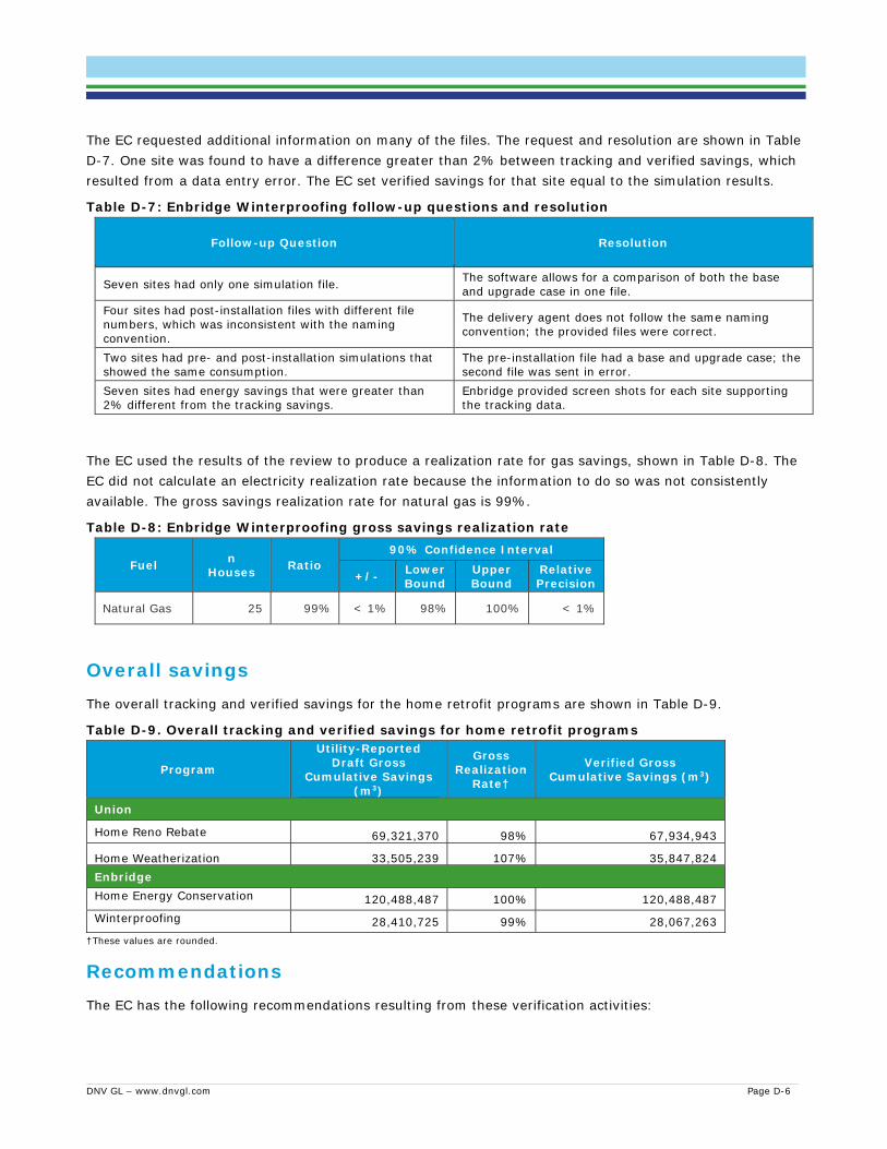
DNV GL – www.dnvgl.com Page D-6
The EC requested additional information on many of the files. The request and resolution are shown in Table D-7. One site was found to have a difference greater than 2% between tracking and verified savings, which resulted from a data entry error. The EC set verified savings for that site equal to the simulation results.
Table D-7: Enbridge Winterproofing follow-up questions and resolution
Follow-up Question Resolution
Seven sites had only one simulation file. The software allows for a comparison of both the base and upgrade case in one file.
Four sites had post-installation files with different file numbers, which was inconsistent with the naming convention.
The delivery agent does not follow the same naming convention; the provided files were correct.
Two sites had pre- and post-installation simulations that showed the same consumption.
The pre-installation file had a base and upgrade case; the second file was sent in error.
Seven sites had energy savings that were greater than 2% different from the tracking savings.
Enbridge provided screen shots for each site supporting the tracking data.
The EC used the results of the review to produce a realization rate for gas savings, shown in Table D-8. The EC did not calculate an electricity realization rate because the information to do so was not consistently available. The gross savings realization rate for natural gas is 99%.
Table D-8: Enbridge Winterproofing gross savings realization rate
Fuel n Houses Ratio
90% Confidence Interval
+/- Lower Bound
Upper Bound
Relative Precision
Natural Gas 25 99% < 1% 98% 100% < 1%
Overall savings The overall tracking and verified savings for the home retrofit programs are shown in Table D-9.
Table D-9. Overall tracking and verified savings for home retrofit programs
Program
Utility-Reported Draft Gross
Cumulative Savings (m3)
Gross Realization
Rate†
Verified Gross Cumulative Savings (m3)
Union
Home Reno Rebate 69,321,370 98% 67,934,943
Home Weatherization 33,505,239 107% 35,847,824 Enbridge Home Energy Conservation 120,488,487 100% 120,488,487 Winterproofing 28,410,725 99% 28,067,263
†These values are rounded.
Recommendations The EC has the following recommendations resulting from these verification activities:

DNV GL – www.dnvgl.com Page D-7
Provide both the building simulation file and program output to the evaluation team. The EC was unable to verify all of the tracking savings directly from the simulation files because some simulations could not be run. Providing both the output files and the simulation models would allow the EC to verify savings without additional follow-up.
Review program processes to improve the quality of the tracking data. The EC identified a number of inaccurate savings entries due to data entry mistakes or outdated results. Many of these errors could be avoided through changes in program processes. Consider reviewing and modifying program processes to avoid similar errors in the future.
Provide more explicit support for the major measures installed at each site. For the market-rate programs, the EC could not verify that the deep savings participants had installed two major measures using the photographs provided with the documentation. Consider providing more explicit support for each major measure to eliminate uncertainty.
Consider funding a study to verify the models produced by the delivery agents. An in-depth review of the simulation models is outside the scope of this verification. Consider funding a study to conduct an in-depth review of the models to ensure they conform to standard industry practice.

DNV GL – www.dnvgl.com Page I-4
APPENDIX E. ENERGY SAVINGS KIT VERIFICATION This appendix describes the detailed process used to certify the reported Energy Savings Kit savings for Union. The EC applied the adjustment factors that were identified in previous evaluations, including:
Final Report Following an Impact Evaluation of the Union Gas ESK-Residential Program: Pull Initiative 2014
Final Report Following an Impact Evaluation of the Union Gas ESK Residential Program: Door-to-Door Drop-off Initiative 2014
Final Report Following an Audit of the Union Gas ESK-Helping Homes Conserve-HHC-Program Low-income Initiative 2012
The adjustment factors from these reports are shown in Table E-1. Table E-2 shows the tracking and verified savings for market-rate residential by rate class. Table E-3 shows the tracking and verified savings for Low Income residential by rate class.
Table E-1: Union: adjustment factors for Energy Savings Kits
Kit Measure Adjustment Factor
Pull – Energy-efficient showerhead 55%
Pull – Kitchen faucet aerator 71%
Pull – Bathroom faucet aerator 81%
Pull – Pipe wrap 98%
Door-to-Door – Energy-efficient showerhead 50%
Door-to-Door – Kitchen faucet aerator 68%
Door-to-Door – Bathroom faucet aerator 80%
Door-to-Door – Pipe wrap 95%
Helping Homes Conserve – Showerhead 80%
Helping Homes Conserve – Kitchen faucet aerator 81%
Helping Homes Conserve – Bathroom faucet aerator 86%
Helping Homes Conserve – Pipe insulation 94%

DNV GL – www.dnvgl.com Page E-1
Table E-2: Union: tracking and verified gross energy savings for residential Energy Savings Kits by rate class
Rate class Measure
Draft Utility-Reported Savings
Adjustment Factor
Verified Savings
Annual Gross
Savings (m3)
Cumulative Gross
Savings (m3)
Annual Gross
Savings (m3)
Cumulative Gross
Savings (m3)
M1 South Residential Pstat 5,300 79,500 100% 5,300 79,500
M1 South Residential Pstat 36,146 542,190 100% 36,146 542,190
M1 South Residential Pstat - - 100% - -
M1 South Residential Pstat 11,183 167,745 100% 11,183 167,745
M1 South Residential ESK Pull - Energy-efficient Showerhead 217,580 2,175,800 55% 119,669 1,196,690
M1 South Residential ESK Pull - Kitchen Faucet Aerator 57,164 571,642 71% 40,587 405,866
M1 South Residential ESK Pull - Bathroom Faucet Aerator 31,648 316,480 81% 25,635 256,349
M1 South Residential ESK Pull - Pipe Wrap 153,097 2,296,458 98% 150,035 2,250,529
M1 South Residential ESK D2D - Energy-efficient Showerhead 570,372 5,703,720 50% 285,186 2,851,860
M1 South Residential ESK D2D - Kitchen Faucet Aerator 149,852 1,498,523 68% 101,900 1,018,996
M1 South Residential ESK D2D - Bathroom Faucet Aerator 82,963 829,632 80% 66,371 663,706
M1 South Residential ESK D2D - Pipe Wrap 401,334 6,020,017 95% 381,268 5,719,016
01 North Residential Pstat 1,590 23,850 100% 1,590 23,850
01 North Residential Pstat 10,282 154,230 100% 10,282 154,230
01 North Residential Pstat - - 100% - -
01 North Residential Pstat 1,219 18,285 100% 1,219 18,285
01 North Residential ESK Pull - Energy-efficient Showerhead 81,180 811,800 55% 44,649 446,490
01 North Residential ESK Pull - Kitchen Faucet Aerator 21,328 213,282 71% 15,143 151,430
01 North Residential ESK Pull - Bathroom Faucet Aerator 11,808 118,080 81% 9,564 95,645
01 North Residential ESK Pull - Pipe Wrap 57,121 856,818 98% 55,979 839,682
01 North Residential ESK D2D - Energy-efficient Showerhead - - 50% - -
01 North Residential ESK D2D - Kitchen Faucet Aerator - - 68% - -
01 North Residential ESK D2D - Bathroom Faucet Aerator - - 80% - -
01 North Residential ESK D2D - Pipe Wrap - - 95% - -
Total 1,901,169 22,398,052 N/A 1,361,705 16,882,059

DNV GL – www.dnvgl.com Page E-2
Table E-3: Union: tracking and verified gross energy savings for Home Weatherization Program basic measures by rate class
Rate class Measure
Draft Utility-Reported Savings*
Adjustment Factor
Verified Savings
Annual Gross Savings (m3)
Cumulative Gross Savings
(m3)
Annual Gross
Savings (m3)
Cumulative Gross Savings
(m3)
M1 South Residential HHC - Energy-efficient Showerhead 2-2.5 138 1,380 80% 110 1,104
M1 South Residential HHC - Energy-efficient Showerhead 2.6+ 1,056 10,560 80% 844.80 8,448
M1 South Residential HHC - Kitchen Faucet Aerator 555 5,549 81% 449 4,495
M1 South Residential HHC - Bathroom Faucet Aerator 282 2,816 86% 242 2,422
M1 South Residential HHC - Pipe Wrap 1,084 16,254 94% 1,019 15,279
Total 3,114 36,559 N/A 2,665 31,747

DNV GL – www.dnvgl.com
APPENDIX F. RUNITRIGHT VERIFICATION This appendix describes the detailed process used to certify the reported RunitRight (RiR) savings for Enbridge. The EC reviewed the RunitRight models, energy savings calculations, and related files to identify any concerns regarding the methodology used by the program, and significant risks for savings accuracy. We also identified opportunities for improvement and suggested future evaluation activities.
The EC randomly selected 10 of 28 participating sites for review. The tasks in the file review included:
Data review: Compare savings claimed for the program to the savings stated in the individual spreadsheets.
─ Conclusion: the savings were confirmed to match.
Methodology review: A senior engineer reviewed the calculation methods and independently calculated savings for one site using the raw consumption data and defined program periods.
─ Conclusion: the methodology used by the RiR program to estimate savings is appropriate for the application. No significant concerns were identified by the team; however, the RiR tool does not allow observation of all of the calculations performed. Independently-calculated savings were statistically equivalent to those calculated by the program for the one site reviewed.
Savings review: Evaluation engineers reviewed the spreadsheets, regression models, and supporting documentation for the sample of sites to identify the answers to the following questions:
─ Is the building type correctly identified? ─ How many months were used in the baseline, improvement, and reference periods? ─ What type of model was used? ─ What independent variables were used? ─ What R-squared values were used for the baseline and reference models? ─ What is the p-value? ─ What balance points were used in the baseline and reference models? ─ What are the estimated savings during the reference period? ─ What are the normalized annual savings? ─ Were capital project savings deducted? ─ What percentage of consumption do the savings represent? ─ Were the measures completed as invoiced? ─ Could the measures have resulted in these savings?
Savings risk assessment: The EC assessed the risk of savings accuracy as Low, Normal, or High based on the calculation review completed, a review of the consumption pattern at the facility, and a review of the baseline model used. Three key questions were answered:
─ Based on experience, is the baseline model specification reasonable? ─ Based on experience, is the baseline time period definition reasonable? ─ What is the assessed level of risk for achieving savings?
─ Conclusion: The baseline model specifications and time period definitions were reasonable. One site was assigned Low risk, five were assigned Normal risk and four were assigned High risk.
─ Three of the four high risk facilities were schools. The regression models were a poor fit for the consumption data, resulting in substantial uncertainty in any savings estimate. The EC

DNV GL – www.dnvgl.com
recommends an assessment of other independent variables for schools, such as an in-session/out-of-session variable to capture break periods.
All savings claims were supported by actions at the facility and clear changes in the consumption patterns occurred. The EC’s review supports a savings claim for all sites.
Recommendations The EC has the following recommendations resulting from these verification activities:
Consider additional independent variables when modeling school consumption. The regressions did not fit school consumption effectively. Additional independent variables accounting for break periods may improve the fit.
Provide more information about each site. Include a basic description of the end-use equipment served by the gas meter, such as DHW, heating, or cooking.
Improve the activity documentation. Include the date of each implemented activity in the calculation workbook and site report. Provide both the baseline and installed values; for example, the pre- and post-installation schedule for a schedule reset. Increase the detail of the end use equipment when a single change results in a significant reduction in consumption.
Consider quantifying electric savings through engineering calculations. While billing data may not be available, engineering calculations would help the program demonstrate the full value it is providing.
Consider reviewing the process for selecting the HDD reference temperature. The EC observed multiple sites where the base load consumption was unexpectedly sensitive to the reference temperature. If in error, the result may be negative baseline savings estimates and poor summer regression results.

DNV GL – www.dnvgl.com
APPENDIX G. LOW INCOME MULTI-FAMILY VERIFICATION This appendix describes the detailed process used to verify the percentage of Part 3 participants enrolled in the Enbridge Low Income Building Performance Management (LIBPM) program, which is one of the scorecard metrics. The equation for calculating the metric is:
%
Where:
X is the number of new LIBPM buildings in the current year which have participated in another aspect of the Low Income program in a previous year of the 2012-2014 plan
Y is the number of new LIBPM buildings participating in the current year which have not previously participated in the Low Income program
Z is the number of buildings in the current year which have implemented custom projects other than LIBPM.24
In response to an EC request, Enbridge provide an Excel workbook with the following information:
A sheet describing the calculation and showing the values for x, y, and z as well as the calculation result based on utility-reported data.
A sheet listing the 121 participants in the 2015 LIBPM program, with flags for previous participation
A sheet listing the number of participants installing custom projects in 2015 who did not participate in the LIBPM program.
To verify this information, the EC:
Confirmed that all reported 2015 Low Income Part 9 buildings were included in the LIBPM workbook. We found that 12 buildings were not, but the projects were prescriptive, not custom, so there was no result in the calculation input. The correct z value is 66, as reported by the program
Confirmed the x and y counts of buildings. We confirmed the program (x + y) total of 121 buildings.
Given the information, the EC calculated the following:
% 121
121 6665%
The EC result is the same as the reported utility result.
24 EB-2015-0049 – Enbridge Gas Distribution Inc. – Multi-Year Demand Side Management Plan (2015 to 2020), Exhibit B, Tab 1, Schedule 3, Page 8
of 19.

DNV GL – www.dnvgl.com
APPENDIX H. CUSTOM PROJECT VERIFICATION This appendix describes the detailed process used to determine the CPSV results and how they are applied to the utility-reported gross savings to get verified gross savings. It also describes the process used to determine the free ridership-based study results which are combined with spillover as discussed in APPENDIX N.25
The primary reporting domains in the CPSV / NTG study report do not align to the programs for LRAM and DSMSI. To get the appropriate effective adjustment factors, the EC:
Applied the measure-level CPSV and free ridership ratios to the population of tracking data
Summed the verified cumulative savings across the desired group (program for Resource Acquisition and Low Income; rate class for Large Volume)
Summed the tracking cumulative savings across the same group
Divided the sum of verified gross by the sum of tracking gross and the sum of verified net by the sum of verified gross to get CPSV and free ridership26 adjustments that most closely follow our sample design.
Table H-1 shows the CPSV and free ridership adjustment factors.
Table H-1. Union CPSV and NTG adjustment factors by subset
Program CPSV Adjustment† Free Ridership Adjustment*†
C&I Custom Comm & Inst Buildings 89% 44%
C&I Custom Ag and Greenhouse 97% 41%
C&I Custom Industrial 103% 39%
Low Income Multi-Family Custom 89% 95%
Large Industrial R100 147% 8%
Large Industrial T1 154% 9%
Large Industrial T2 131% 8% †These values are rounded. * This is presented in the form of a NTG ratio based solely on free ridership. Technically, this value is 1 minus free ridership.
To get the appropriate adjustment factors for the Enbridge custom projects, the EC followed the same process. Table H-2 shows the adjustment factors.
25 “2015 Natural Gas Demand Side Management Custom Savings Verification and Free-ridership Evaluation”. Prepared for the Ontario Energy Board.
August 15, 2017. 26 In this analysis, the “free ridership adjustment” is in the form of a NTG ratio based on free ridership alone. It is more accurate to say that the
value calculated by dividing the sum of verified net by the sum of verified gross is 1 minus the free ridership value.

DNV GL – www.dnvgl.com
Table H-2. Enbridge CPSV and NTG adjustment factors
Program CPSV Adjustment† Free Ridership Adjustment*†
Custom Commercial 91% 17%
C&I Custom New Construction 91% 18%
Custom Multi-family 91% 35%
Custom Industrial Ag 99% 28%
Custom Industrial 100% 33%
RunitRight 100% 50% †These values are rounded. * This is presented in the form of a NTG ratio based solely on free ridership. Technically, this value is 1 minus free ridership.
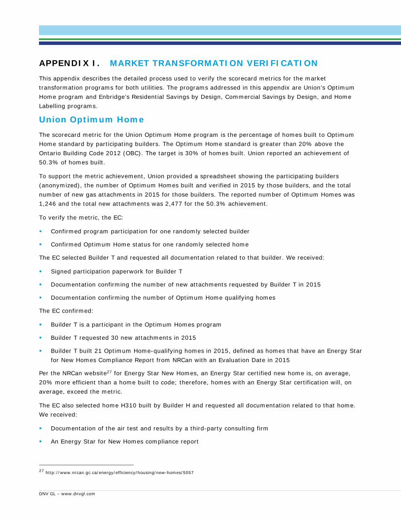
DNV GL – www.dnvgl.com
APPENDIX I. MARKET TRANSFORMATION VERIFICATION This appendix describes the detailed process used to verify the scorecard metrics for the market transformation programs for both utilities. The programs addressed in this appendix are Union’s Optimum Home program and Enbridge’s Residential Savings by Design, Commercial Savings by Design, and Home Labelling programs.
Union Optimum Home The scorecard metric for the Union Optimum Home program is the percentage of homes built to Optimum Home standard by participating builders. The Optimum Home standard is greater than 20% above the Ontario Building Code 2012 (OBC). The target is 30% of homes built. Union reported an achievement of 50.3% of homes built.
To support the metric achievement, Union provided a spreadsheet showing the participating builders (anonymized), the number of Optimum Homes built and verified in 2015 by those builders, and the total number of new gas attachments in 2015 for those builders. The reported number of Optimum Homes was 1,246 and the total new attachments was 2,477 for the 50.3% achievement.
To verify the metric, the EC:
Confirmed program participation for one randomly selected builder
Confirmed Optimum Home status for one randomly selected home
The EC selected Builder T and requested all documentation related to that builder. We received:
Signed participation paperwork for Builder T
Documentation confirming the number of new attachments requested by Builder T in 2015
Documentation confirming the number of Optimum Home qualifying homes
The EC confirmed:
Builder T is a participant in the Optimum Homes program
Builder T requested 30 new attachments in 2015
Builder T built 21 Optimum Home-qualifying homes in 2015, defined as homes that have an Energy Star for New Homes Compliance Report from NRCan with an Evaluation Date in 2015
Per the NRCan website27 for Energy Star New Homes, an Energy Star certified new home is, on average, 20% more efficient than a home built to code; therefore, homes with an Energy Star certification will, on average, exceed the metric.
The EC also selected home H310 built by Builder H and requested all documentation related to that home. We received:
Documentation of the air test and results by a third-party consulting firm
An Energy Star for New Homes compliance report
27 http://www.nrcan.gc.ca/energy/efficiency/housing/new-homes/5057
DNV GL – www.dnvgl.com
A workbook showing the Energy Star for New Homes Energy Advisor Verification Checklist
The EC confirmed:
Home H310 built by Builder T conforms to Optimum Home requirements.
The home has gas water and space heat.
As a result of this review, the EC confirms the reported Optimum Home scorecard metric of 50.3%.
Enbridge Residential Savings by Design The scorecard metrics for the Enbridge Residential Savings by Design (RSBD) program are the number of builders enrolled in the program and the number of homes built to RSBD standard. The RSBD standard is greater than 25% above the Ontario Building Code 2012 (OBC). The targets are 18 builders enrolled and 1,111 homes built. Enbridge reported achievements of 19 builders enrolled and 1,987 homes built. By definition, an enrolled builder must have built a minimum of 50 homes in the previous year to qualify.
To support the metric achievement, Enbridge provided a spreadsheet showing the participating builders, confirmation that they built more than 50 homes in the prior year, and the integrated design process (IDP) date for each builder. Enbridge also provided a workbook listing the houses built to RSBD standard, by builder, that received an incentive, and the number of reported houses, by builder, self-reported through letters.
To verify the metrics, the EC:
Confirmed program participation for one randomly selected builder
Confirmed RSBD status for one randomly selected home
The EC selected Builder #65 and requested all documentation related to that builder. We received:
A copy of the builder commitment form, which confirms that the builder completed more than 50 homes in the previous year
Notes from the visioning session
The agenda from the Integrated Design Charrette
The findings from the integrated design process (IDP)
The EC confirmed:
Builder #65 is a participant in the RSBD program and joined in 2015
Builder #65 self-reported a minimum of 50 homes build in 2014
Builder #65 participated in the visioning workshop and IDP session and designed a townhome that is 27.6% better than OBC
The EC also selected home HL88 and requested all documentation related to that home. We received:
Documentation of the air test and results by a third-party consulting firm
An SBD modelling summary sheet
A HOT2000 model file

DNV GL – www.dnvgl.com
The EC confirmed:
Home RSBD conforms to RSBD requirements.
As a result of this review, the EC confirms the reported RSBD scorecard metrics of 19 builders and 1,987 homes built.
Enbridge Commercial Savings by Design The scorecard metric for the Enbridge Commercial Savings by Design (CSBD) program is the number of developments enrolled in the program. The target is 18 new developments enrolled. Enbridge reported an achievement of 24 developments enrolled. To qualify, the development must exceed 50,000 square feet in size.
To support the metric achievement, Enbridge provided a spreadsheet showing the participating builders and the developments that were enrolled in 2015.
To verify the metrics, the EC confirmed program participation for one randomly selected developer. The EC selected the development by Builder #54 and requested all documentation related to that builder and development. We received:
A copy of the application form for the builder
Pre-meeting notes from the ½-day visioning session with the builder
A report on the findings from the integrated design workshop.
An email confirming that the size of the development is greater than 50,000 square feet.
The EC confirmed:
Builder #54 is a participant in the CSBD program
Builder #54 participated in the visioning workshop and IDP session and designed a development that is 34.2% better than OBC
As a result of this review, the EC confirms the reported CSBD scorecard metric of 24 developments enrolled.
Enbridge Home Labelling The scorecard metrics for the Enbridge Home Labelling program are the number of annual listings by realtors committed to the program and the number of ratings performed. The targets are 5,000 listings and 4,500 ratings performed. Enbridge reported achievements of 41,650 listings and 336 ratings performed.
To support the metric achievement, Enbridge provided a spreadsheet that listed all of the addresses that received a Home Labelling rating and another spreadsheet showing the number of listings represented by each committed realtor. To verify the number of addresses, the EC:
Confirmed program participation for one randomly selected realtor
Confirmed the number of listings represented by that realtor
Confirmed the ratings completed by that realtor
The EC selected a realtor and requested all documentation related to that office. We received:

DNV GL – www.dnvgl.com
The brokerage commitment form
Proof of labelling at three addresses related to that realtor
An updated labelling tracking spreadsheet
In assembling the documentation for the requested realtor, Enbridge discovered a duplicate entry. They reviewed all of the documentation in the program and found three duplicates in total, reducing the number of completed ratings to 333.
The EC confirmed:
The realtor is a participant in the Home Labelling program
The realtor represents 2000 listings per year.
The builder completed three ratings in 2015
As a result of this review, the EC confirms the reported Home Labelling scorecard metric of 333 ratings and 41,650 listings.

DNV GL – www.dnvgl.com Page J-1
APPENDIX J. REVIEW OF LRAM AND DSMSI CALCULATIONS This appendix describes the EC team’s review of the lost revenue adjustment mechanism (LRAM) and demand side management shareholder incentive (DSMSI) calculations.
The LRAM calculation is based on:
The verified net natural gas savings (in annual cubic meters) by rate class
The delivery cost of the natural gas by rate class
The month in which the measure was installed
The DSMSI calculation is based on:
The actual program achievements compared to the target metrics for that scorecard
The weight placed on each metric within each scorecard
The maximum incentive achievable for that scorecard
The detailed DSMSI calculations for each utility are outlined in the following sections. The EC was unable to identify or locate the source of approval for the calculations. The two utility calculations are very similar and follow the same principles and do not violate the general direction approved by the OEB; therefore, the EC will use the methodology provided by the utilities.
The EC confirmed the lower band, upper band, target metric, and weights for both utilities.
LRAM: Union Union delivered a calculation workbook for LRAM which includes the tracking savings, an input sheet for adjustment factors, and a sheet with avoided costs. The LRAM calculation for a given rate class and month is as follows:
The verified net energy savings for the given rate class and month are summed.
The savings are multiplied by the following calculation, which pro-rates the savings for the remainder of the year and divides by 1000 to produce the savings volume in thousands of cubic meters.
12 # 112 1000
For example, the savings for a particular rate class for measures installed in July would be multiplied by:
12 7 112 1000
612
11000
The equation allots energy savings from that project to half of the year and converts it to thousands of cubic meters.
The savings from each month are summed across rate classes and multiplied by an annual delivery rate for that class to get the revenue impact for each class.
The revenue impact from each rate class is summed across classes to get the total LRAM for Union. Only the contract rate cases are included in the LRAM calculations.
DNV GL – www.dnvgl.com Page J-2
LRAM: Enbridge Enbridge delivered a calculation workbook for LRAM which includes the tracking savings, a sheet to calculate the budgeted LRAM values, a sheet to calculate the actual LRAM values, and a sheet showing the distribution margin rates. The actual LRAM calculation for a given rate class and month is as follows:
The annual net savings are summed by rate class and sector and the month in which the measure was installed.
The savings by rate class and sector and month are divided by 12 to produce monthly savings and applied to each month from the installation month through the rest of the year.
The savings are summed across months for each sector.
The savings are summed across sectors for each rate class.
The Enbridge calculation workbook does not calculate the actual LRAM, it calculates the LRAM variance, which shows the difference between the actual LRAM and the budgeted LRAM for the year.28 To calculate the actual LRAM (consistent with the Union calculation above), the EC multiplied the actual net savings summed across sectors for each rate by the distribution margin to get LRAM.
The revenue impact from each rate class is summed across classes to get the total LRAM for Enbridge. Only the contract rate cases are included in the LRAM calculations.
28 After the draft report was produced, Enbridge provided a calculation workbook that included the actual LRAM in addition to the LRAM variance.

DNV GL – www.dnvgl.com Page J-3
DSMSI: Union The Union tracking workbook includes a sheet for calculating the DSMSI based on utility-reported results. The DSMSI is calculated based on the metric achievement relative to the target level within an acceptable ± band. The Union targets, upper and lower bands, and weights are shown in Table J-1. The EC verified the metrics, upper and lower bands, and weights shown in the table.
Table J-1. Union’s 2015 scorecard targets, lower band, upper band, and weight
Scorecard Lower Band 2015 Target Upper Band Weight
Union
Resource Acquisition 612,421,364 CCM
934 participants
7.88%
816,561,818 CCM
1,245 deep savings participants
8.88% of commercial whole building
natural gas use saved
1,020,702,273 CCM
1,556 participants
9.88%
90%
5%
5%
Large Volume 154,692,013 CCM
772,381,040 CCM
206,256,017 Rate 1 CCM
1,029,841,387 Rate T2/100 CCM
257,820,021 CCM
1,287,301,734 CCM
60%
40%
Low Income 19,500,000 CCM
13,200,000 CCM
26,000,000 single family CCM
17,600,000 multi-family CCM
32,500,000 CCM
22,000,000 CCM
60%
40%
Market Transformation 25% 30% of homes built by participating builders were
20% more efficient than OBC
35% 100%

DNV GL – www.dnvgl.com Page J-4
The shareholder incentive calculation in the Union tracking workbook first defines a % Achievement.
If the achieved metric is less than the target, % achievement is calculated:
% 1 0.5 ∗
1
1 0.5 ∗
If the achieved metric is greater than the target, % achievement is calculated:
% 1.5 1 ∗
1.5
1.5 1 ∗
The % Achievement is multiplied by the weight to produce % Contribution, which is summed. The summed value is used to calculated the achieved shareholder incentive using:
If the sum of % Contribution is greater than 0.5 and less than 1, then:
0.8 ∗ % 0.4 ∗
If the sum of % Contribution is greater than or equal to 1 and less than or equal to 1.5, then:
1.2 ∗ % 0.8 ∗
If the sum of % Contribution is greater than 1.5, then:
1.2 ∗ 1.5 0.8 ∗
Otherwise the maximum shareholder incentive is zero.

DNV GL – www.dnvgl.com Page J-5
DSMSI: Enbridge The Enbridge tracking workbook includes a sheet for calculating the DSMSI based on utility-reported results. The DSMSI is calculated based on the metric achievement relative to the target level within an acceptable ± band. The Enbridge targets, upper and lower bands, and weights are shown in Table J-2. The EC verified the metrics, upper and lower bands, and weights shown in the table.
Table J-2. Enbridge’s 2015 scorecard targets, lower band, upper band, and weight
Scorecard Lower Band 2015 Target Upper Band Weight
Enbridge
Resource Acquisition 758,900,000 CCM
571 participants
1,011,900,000 CCM
762 deep savings participants
1,264,900,000 CCM
952 participants
92%
8%
Low Income 18,100,000 CCM
51,600,000 CCM
30%
24,100,000 single family CCM
68,700,000 multi-family CCM
40% of Part 3 in LIBPM
30,200,000 CCM
86,000,000 CCM
50%
50%
45%
5%
Savings by Design
Residential
13 builders
833 homes
18 builders enrolled
1,111 homes built by participating builders were
20% more efficient than OBC
22 builders
1,389 homes
60%
40%
Savings by Design
Commercial
11 developments 18 developments enrolled 24 developments 100%
Home Labelling No listings
2,250 ratings
5,001 total listings from committed realtors
4,500 ratings performed
10,001 listings
6,750 ratings
50%
50%

DNV GL – www.dnvgl.com Page J-6
The shareholder incentive calculation in the Enbridge tracking workbook first defines a Score.
If the achieved metric is less than or equal to the target, Score is calculated:
10.5 ∗
If the achieved metric is greater than the target, Score is calculated:
10.5 ∗
The Score is multiplied by the weight and summed to produce the Weighted Score. The Weighted Score is used to calculated the achieved shareholder incentive using:
If the Weighted Score is less than 0.5 then the shareholder incentive is zero.
If the Weighted Score is greater than or equal to 0.5 and less than 1, then:
0.4 ∗
∗ 0.50.5
If the Weighted Score is greater than or equal to 1 and less than or equal to 1.5, then:
∗ 1
0.5
If the Weighted Score is greater than 1.5 then the shareholder incentive is equal to the maximum shareholder incentive.
Recommendations The EC has the following recommendation resulting from these verification activities:
Provide a detailed explanation for the DSMSI calculation for review by the EC and OEB. The EC was unable to locate a source document that supports the utility calculation of DSMSI. Given the importance of the shareholder incentive, it is appropriate to have a clearly defined and detailed explanation of how it is calculated.

DNV GL – www.dnvgl.com Page K-1
APPENDIX K. LRAM AND DSMSI: DETAILED CALCULATIONS This appendix describes the detailed process used to calculate the DSMSI and LRAM for both utilities.
Union DSMSI The metrics that affect the Union DSMSI include:
Resource Acquisition cumulative net savings
Low Income cumulative net savings
Large Volume cumulative net savings
Non-savings metrics:
─ The number of deep savings participants in the Home Reno Rebate program ─ The average percent of whole-building energy use saved by C&I customers ─ The number of homes built greater than 20% above Ontario Building Code by participating
Optimum Home builders
To verify the savings metrics, the EC applied the program-level results from the previous appendices. Table K-1 shows the location of the detailed explanation for each program.
Table K-1. Union source of detailed explanation of adjustment factors
Portfolio Component Location of Detailed Explanation
Ag and Greenhouse APPENDIX H APPENDIX N
Commercial and Institutional Buildings APPENDIX H APPENDIX N
Industrial APPENDIX H APPENDIX N
Energy Savings Kit APPENDIX E
Home Reno Rebate APPENDIX D
Commercial and Industrial Prescriptive APPENDIX C
Low Income Multi-family (custom projects) APPENDIX H
Low Income Multi-family (prescriptive projects) APPENDIX C
Home Weatherization Program APPENDIX D
Large Volume (custom projects) APPENDIX H APPENDIX N
Large Volume (prescriptive projects) APPENDIX C
The analysis to produce the verified savings from the tracking savings differed by the type of project.
For custom projects (those discussed in APPENDIX H), the appropriate CPSV adjustment factor was applied to the annual and cumulative gross tracking savings to produce annual and cumulative gross

DNV GL – www.dnvgl.com Page K-2
verified savings. The appropriate NTG adjustment factor, including the provisional spillover value discussed in APPENDIX N, was applied to the annual and cumulative gross verified savings to produce annual and cumulative net verified savings.
For the home renovation projects (those discussed in APPENDIX D), the appropriate natural gas adjustment factor was applied to the annual gross tracking savings to produce annual gross verified savings. The annual gross verified savings were multiplied by the program-assumed measure life to produce cumulative gross verified savings. Both the annual gross and cumulative gross verified savings were multiplied by the complement of the program-assumed free-ridership percentage to produce annual and cumulative verified net savings.
For the Energy Savings Kit projects (those discussed in APPENDIX E), the EC calculated the measure-level annual and cumulative gross verified savings, summed them to the technology level (such as showerheads or pipe wrap), and divided the cumulative gross verified savings by the cumulative gross tracking savings to produce a technology-level gross adjustment factor. The annual and cumulative gross verified savings were multiplied by the complement of the program-assumed free-ridership percentage to produce annual and cumulative net verified savings.
For the remaining prescriptive projects (those discussed in APPENDIX C), the EC multiplied the annual and cumulative gross tracking savings by the appropriate adjustment factor to produce annual and cumulative gross verified savings. The annual and cumulative gross verified savings were multiplied by the complement of the program-assumed free-ridership percentage to produce annual and cumulative net verified savings.
Program-level adjustment factors were determined by first summing the gross cumulative verified and tracking savings and net cumulative verified and tracking savings across the program, then dividing the verified by the tracking result to get the adjustment factor.
Table K-3 shows the Union verified 2015 savings by scorecard and program.
For the non-savings metrics, the EC determined the verified metric as described in the previous appendices. Table K-2 shows the location of the detailed explanation for each metric and the verified value.
Table K-2. Union source of detailed explanation of final non-savings metrics and verified value
Metric Location of Detailed Explanation Verified Value
Number of residential deep savings participants APPENDIX D 2,529
Percent of whole-building energy use saved APPENDIX C 8.08%
Percent of qualifying homes by Optimum Home builders APPENDIX I 50.3%

DNV GL – www.dnvgl.com Page K-3
Table K-3. Union’s verified 2015 savings by scorecard and program
Program
Draft Utility-Reported Savings* Verification Results Verified Savings
Gross Annual (m3)
Gross Cumulative
(m3)
Net Annual (m3)
Net Cumulative
(m3)
Gross Realization
Rate†
Net-to-Gross†
Gross Cumulative
(m3)
Net Cumulative
(m3) Resource Acquisition
C&I Prescriptive 10,659,544 208,919,006 9,283,248 182,411,887 100% 87% 208,919,006 182,411,887 C&I Custom Ag and Greenhouse 41,708,475 611,477,005 19,185,899 281,279,422 97% 44% 592,368,700 262,534,051
C&I Custom Comm & Inst Buildings 16,527,002 268,582,354 7,602,421 123,547,883 89% 47% 239,199,444 112,642,330
C&I Custom Industrial 36,329,242 593,859,359 16,711,451 273,175,305 103% 43% 612,343,937 260,640,852
Energy Savings Kit 1,901,169 22,398,052 1,644,462 19,567,373 75% 88% 16,882,059 14,800,935
Home Reno Rebate 3,828,386 69,321,370 3,254,128 58,923,165 98% 85% 67,934,943 57,744,701
Total RA 110,953,818 1,774,557,146 57,681,609 938,905,035 98% 51% 1,737,648,089 890,774,755†
Large Volume
Large Industrial-T1 12,469,705 171,240,007 5,743,536 78,919,835 154% 13% 263,624,641 33,725,518
Large Industrial-T2 83,288,363 1,002,106,837 38,382,453 462,016,235 131% 11% 1,309,850,111 147,448,803
Large Industrial-R100 11,155,712 80,624,184 5,131,627 37,087,125 147% 12% 118,331,969 13,695,699
Total LV 106,913,780 1,253,971,028 49,257,616 578,023,195 135% 12% 1,691,806,721 194,870,020
Low Income
Low Income Multi-family 957,046 17,840,732 909,194 16,948,695 96% 95% 17,193,011 16,333,361
Home Weatherization 1,341,946 33,505,239 1,341,913 33,504,841 107% 100%† 35,847,824 35,847,426
Total LI 2,298,992 51,345,970 2,251,107 50,453,536 103% 98% 53,040,835 52,180,787 * The utility-reported values reflect the savings presented in the utility’s tracking workbook, not in the draft 2015 report. The utility changed the energy savings values for some projects after
submitting the 2015 report but before delivering the data for evaluation, resulting in a small change. †These values are rounded.

DNV GL – www.dnvgl.com Page K-4
The EC entered the appropriate metrics into the Union scorecard calculator. The resulting shareholder incentive results can be found in Table K-4. The total shareholder incentive is $7,039,894.
Table K-4. Union DSMSI results Scorecard DSMSI
Resource Acquisition $4,010,638
Low Income $2,462,534
Large Volume $0
Market Transformation $566,721
Total $7,039,894
Enbridge DSMSI The metrics that affect the Enbridge DSMSI include:
Resource Acquisition cumulative net savings
Low Income cumulative net savings
Non-savings metrics:
─ The number of deep savings participants in the Home Energy Conservation program ─ The percentage of Part 3 participants that are also in the LIBPM program ─ The number of builders participating in the RSBD program ─ The number of homes built greater than 25% above Ontario Building Code by participating RSBD
builders ─ The number of builders participating in the CSBD program ─ The number of listings represented by realtors in the Home Labelling program ─ The number of ratings in the Home Labelling program
To verify the savings metrics, the EC applied the program-level results from the previous appendices. Table K-5 shows the location of the detailed explanation for each program.

DNV GL – www.dnvgl.com Page K-5
Table K-5. Enbridge source of detailed explanation of adjustment factors
Portfolio Component Location of Detailed Explanation
Home Energy Conservation APPENDIX D
Commercial Prescriptive APPENDIX C
Commercial Custom APPENDIX H APPENDIX N
RunitRight APPENDIX F APPENDIX H APPENDIX N
Multi-family APPENDIX H APPENDIX N
New Construction APPENDIX H APPENDIX N
Industrial Custom APPENDIX H APPENDIX N
Industrial Prescriptive APPENDIX C
Industrial Agriculture APPENDIX H APPENDIX N
Low Income Multi-family (prescriptive projects) APPENDIX C
Low Income Multi-family (custom projects) APPENDIX H
Low Income Single Family: Winterproofing APPENDIX D
Low Income Single Family non-Winterproofing APPENDIX C
The analysis to produce the verified savings from the tracking savings differed by the type of project.
For custom projects (those discussed in APPENDIX H), the appropriate CPSV adjustment factor was applied to the annual and cumulative gross tracking savings to produce annual and cumulative gross verified savings. The appropriate NTG adjustment factor, including the provisional spillover value discussed in APPENDIX N, was applied to the annual and cumulative gross verified savings to produce annual and cumulative net verified savings.
For the home renovation projects (those discussed in APPENDIX D), the appropriate natural gas adjustment factor was applied to the annual gross tracking savings to produce annual gross verified savings. The annual gross verified savings were multiplied by the program-assumed measure life to produce cumulative gross verified savings. Both the annual gross and cumulative gross verified savings were multiplied by the complement of the program-reported free-ridership percentage to produce annual and cumulative net verified savings.
For the RunitRight projects (those discussed in APPENDIX F), the EC applied the gross savings verification adjustment from APPENDIX F to the annual and cumulative gross tracking savings to produce annual and cumulative gross verified savings. The appropriate NTG adjustment factor (from APPENDIX H and APPENDIX N) was applied to the annual and cumulative gross verified savings to produce annual and cumulative net verified savings.

DNV GL – www.dnvgl.com Page K-6
For the remaining prescriptive projects (those discussed in APPENDIX C), the EC calculated the verified gross annual and cumulative savings for the population of measures. The verified savings were summed into groupings corresponding to the program-reported free-ridership rate. The annual and cumulative verified net savings were produced by multiplying the verified gross savings by the complement of the program-reported free-ridership rate. The final gross savings adjustment factor was calculated by dividing the cumulative gross verified savings by the cumulative gross tracking savings.
Program-level adjustment factors were determined by first summing the gross cumulative verified and tracking savings and net cumulative verified and tracking savings across the program, then dividing the verified by the tracking result to get the adjustment factor.
Table K-7 shows the Enbridge verified 2015 savings by scorecard and program.
For the non-savings metrics, the EC determined the final metric as described in the previous appendices. Table K-6 shows the location of the detailed explanation for each metric and the verified value.
Table K-6. Enbridge source of detailed explanation of final non-savings metrics and verified value
Metric Location of Detailed Explanation Verified Value
Number of residential deep savings participants APPENDIX D 5,646
Percent of Part 3 in LIBPM APPENDIX G 65%
Number of builders in RSBD APPENDIX I 19
Number of qualifying homes in RSBD APPENDIX I 1,987
Number of developments in CSBD APPENDIX I 24 Number of listings represented by Home Labelling realtors APPENDIX I 41,650
Number of Home Labelling listings APPENDIX I 333

DNV GL – www.dnvgl.com Page K-7
Table K-7. Enbridge’s verified 2015 savings by scorecard and program
Program
Draft Utility-Reported Savings* Verification Results Verified Savings Gross
Annual (m3)
Gross Cumulative
(m3)
Net Annual (m3)
Net Cumulative
(m3)
Gross Realization
Rate**†
Net-to-Gross†
Gross Cumulative
(m3)
Net Cumulative
(m3) Resource Acquisition
Home Energy Conservation 7,956,225 120,488,487 6,762,791 102,415,214 100% 85% 120,488,487 102,415,214
Prescriptive Commercial 6,858,765 117,938,979 5,750,534 98,693,722 97% 85% 114,897,650 97,416,428
Custom Commercial 14,007,133 210,800,594 12,326,277 185,504,523 91% 21% 192,840,383 40,105,236
RunitRight 536,821 2,684,105 536,821 2,684,105 100% 53% 2,684,105 1,434,923
Custom Multi-family 7,363,563 152,593,766 5,890,850 122,075,013 91% 38% 139,592,777 53,699,388
C&I Custom New Construction 4,091,779 102,294,475 3,027,916 75,697,912 91% 22% 93,578,986 20,231,777
Custom Industrial 22,195,244 336,500,502 11,097,622 168,250,251 100% 36% 337,417,582 122,387,967
Prescriptive Industrial 561,521 10,826,785 398,824 7,593,008 100% 70% 10,826,785 7,593,008
Custom Industrial Ag 611,305 7,856,800 366,783 4,714,080 99% 32% 7,815,133 2,467,184
Total RA 64,182,357 1,061,984,493 46,158,419 767,627,826 96% 44% 1,020,141,888 447,751,124†
Low Income
LI Multi-Family 3,425,023 69,505,240 3,397,177 69,226,782 92% 100% 63,969,354 63,969,354
Single Family 1,146,633 28,410,725 1,139,959 28,343,978 99% 100% 28,067,263 28,067,263
Total LI 4,571,656 97,915,965 4,537,136 97,570,759 94% 100% 92,036,617 92,036,617 * The utility-reported values reflect the savings presented in the utility’s tracking workbook, not in the draft 2015 report. The utility changed the energy savings values for some projects after
submitting the 2015 report but before delivering the data for evaluation, resulting in a small change. ** The gross realization rate for C&I prescriptive, single family low income, and multi-family low income includes the removal rate for some measures, which was previously included in the net-
to-gross adjustment. See APPENDIX C for more detail. †These values are rounded.

DNV GL – www.dnvgl.com Page K-8
The EC entered the appropriate metrics into the Enbridge scorecard calculator. The resulting shareholder incentive results can be found in Table K-8. The total shareholder incentive is $6,207,339.
Table K-8. Enbridge DSMSI results Scorecard DSMSI
Resource Acquisition $2,612,431
Low Income $1,483,748
Residential Savings by Design $1,076,493
Commercial Savings by Design $418,269
Home Labelling $616,397
Total $6,207,339
Union LRAM The inputs into the Union LRAM calculation are:
Verified net annual energy savings by rate class and installation month using the best available information. When the installation month was in the previous year (2014), the EC assigned the savings to January.
The annual delivery rate for each rate class.
To determine verified savings by month and rate class, the EC completed the following activities:
Prescriptive savings: The EC identified the best available information for estimating energy savings, which is the currently (in 2017) approved TRM. The EC determined the prescriptive savings using the new source, summed the annual gross verified savings by month, rate class, and free rider rate, then applied the appropriate free rider rate to get annual verified net savings, and summed across the rate class to get annual verified net savings by month and rate class.
Custom savings: The EC applied the measure-level CPSV and NTG ratios (which is the best available information) to the population of tracking data, then summed the verified annual savings across measures to the project level. The project-level verified annual net savings were summed by month and rate class.
Combined savings: The EC summed prescriptive and custom savings by month and rate class to get the appropriate inputs to the LRAM calculation.
The EC input the summed savings by month and rate class to the utility calculator to produce the appropriate LRAM, shown in Table K-10. Table K-9 shows the results of the Union LRAM calculation by rate class.

DNV GL – www.dnvgl.com Page K-9
Table K-9. Union LRAM results
Rate Class Utility-Reported Draft LRAM Verified LRAM
M4 Industrial $77,105 $74,681
M5 Industrial $38,366 $36,890
M7 Industrial $33,512 $32,272
T1 Industrial $2,789 $1,462
T2 Industrial $1,050 $361
20 Industrial $7,002 $6,808
100 Industrial $5,578 $1,894
Total $165,411 $154,368

DNV GL – www.dnvgl.com Page K-10
Table K-10. Union LRAM inputs: annual net savings by rate class and install month Annual Savings, m3
Rate Class January February March April May June July August September October November December Total M4
Industrial 3,083,002 1,999,552 187,818 521,549 286,759 504,735 322,165 574,183 1,005,348 1,179,650 336,789 1,641,224 11,642,773
M5 Industrial 552,813 196,382 39,286 91,241 34,021 153,741 231,145 353,937 245,625 394,109 673,021 779,719 3,745,040
M7 Industrial 4,120,364 1,561,302 147,127 1,111,725 959,007 290,188 735,902 967,723 1,145,242 2,309,053 1,520,403 14,868,035
T1 Industrial 921,276 43,574 252,526 809,025 24,584 39,544 300,828 135,662 112,031 345,195 2,993,246
T2 Industrial 1,996,914 199,678 105,398 197,957 565,058 1,812,816 864,661 6,032,584 1,351,311 13,126,378
20 Industrial 338,561 116,316 44,138 157,478 212,997 942,094 111,890 226,313 641,954 2,791,740
100 Industrial 67,431 4,834 1,076,988 18,672 15,384 349,502 113,806 95,811 1,742,430
Total 11,012,930 3,757,237 601,552 2,225,691 2,194,210 2,405,670 1,560,426 3,719,206 4,806,085 5,199,624 9,654,757 3,772,254 50,909,642

DNV GL – www.dnvgl.com Page K-11
Enbridge LRAM The inputs into the Enbridge LRAM calculation are:
Verified net annual energy savings by rate class and installation month using the best available information
The annual delivery rate for each rate class
To determine verified savings by month and rate class, the EC completed the following activities:
Prescriptive savings: The EC identified the best available information for estimating energy savings, which is the currently (in 2017) approved TRM. The EC determined the prescriptive savings using the new source, summed the annual gross verified savings by month, rate class, and free rider rate, then applied the appropriate free rider rate to get annual verified net savings, and summed across the rate class to get annual verified net savings by month and rate class.
Custom savings: The EC applied the measure-level CPSV and NTG ratios (which is the best available information) to the population of tracking data, then summed the verified annual savings across measures to the project level. The project-level verified annual net savings were summed by month and rate class.
Combined savings: The EC summed prescriptive and custom savings by month and rate class to get the appropriate inputs to the LRAM calculation.
The EC put the summed savings by month and rate class, shown in Table K-12 into our own calculator to produce the appropriate LRAM. Table K-11 shows the results of the Enbridge LRAM calculation by rate class.
Table K-11. Enbridge LRAM results
Rate Class LRAM
110 $11,769
115 $2,932
135 $239
145 $876
170 $590
Total $16,405

DNV GL – www.dnvgl.com Page K-12
Table K-12. Enbridge LRAM inputs: annual net savings by rate class and install month
Annual Savings, m3
Rate Class January February March April May June July August September October November December Total
110 19,427 132,111 545,957 36,267 91,432 2,278,880 54,604 3,158,677
115 50,493 1,824 49,302 66,086 1,685,999 20,492 1,874,196
135 106,396 10,636 117,031
145 12,443 12,066 5,690 236,109 41,538 307,846
170 105,506 966 7,373 423,287 65,616 602,748
Total 0 0 19,427 50,493 0 146,378 663,530 86,536 0 170,581 4,730,670 192,885 6,060,499

DNV GL – www.dnvgl.com Page L-1
APPENDIX L. PROGRAM SPENDING This section reports additional program spending detail for Union and Enbridge.
Union Table L-1. Union Resource Acquisition scorecard spending
Spending Area Actual Spent
Residential Residential Incentives $3,552,367 Residential Administration $527,197 Residential Evaluation $397,650 Residential Promotion Costs $972,997 Total Residential Program $5,450,210
Commercial/Industrial Commercial/Industrial Incentives $7,547,776 Commercial/Industrial Administration $2,924,084 Commercial/Industrial Evaluation $100,200 Commercial/Industrial Promotion Costs $796,336 Total Commercial/Industrial Program $11,368,397
Table L-2. Union Large Volume scorecard spending
Spending Area Actual Spent
Large Industrial T1/T2/R100 Incentives $2,219,151 Large Industrial T1/T2/R100 Administration $863,933 Large Industrial T1/T2/R100 Evaluation $122,498 Large Industrial T1/T2/R100 Promotion Costs $4,134 Total Large Industrial T1/T2/R100 Program $3,209,716
Table L-3. Union Low Income scorecard spending
Spending Area Actual Spent
Low Income Incentives $5,449,462 Low Income Administration $859,796 Low Income Evaluation $196,171 Low Income Promotion Costs $1,195,605 Total Low Income $7,701,035

DNV GL – www.dnvgl.com Page L-2
Table L-4. Union Market Transformation scorecard spending
Spending Area Actual Spent
Optimum Home Incentives $736,173 Optimum Home Administration $386,703 Optimum Home Promotion Costs $282,464 Total Optimum Home Program $1,405,340
Table L-5. Union portfolio budget spending for research, evaluation, and administration
Spending Area Residential C&I Low Income Large Industrial
Market Trans-formation Total
% of Overall 19% 39% 26% 11% 5% 100%
Research $61,568 $128,422 $86,994 $36,258 $15,875 $329,116
Evaluation $98,214 $204,861 $138,774 $57,840 $25,324 $525,012
Administration $409,671 $854,517 $578,856 $241,262 $105,634 $2,189,940
Total DSM Budget $569,452 $1,187,799 $804,624 $335,359 $146,834 $3,044,068
Enbridge Table L-6. Enbridge program costs for Resource Acquisition
Resource Acquisition OEB-Approved Budget
Actual Spending
Indirect Direct Total
Residential
HEC $1,872,720 $8,340,428 $1,021,867 $9,362,295
Residential Total $1,872,720 $8,340,428 $1,021,867 $9,362,295
Commercial
Comm Prescriptive $759,387 $0 $759,387
Comm Custom $1,647,605 $785,017 $2,432,622
RunitRight -$12,480 $1,471,376 $1,458,896
Multi residential (Comm) $1,485,719 $41,350 $1,527,069
New Construction (Comm) $43,624 $125 $43,749
Commercial Total $8,252,370 $3,923,856 $2,297,867 $6,221,724
Industrial Custom Industrial (excl. Agriculture)
$1,450,240 $581,814 $2,032,054
Prescriptive Industrial
$27,150 $0 $27,150
Agriculture $96,698 $10,805 $107,502
Industrial Total $4,318,700 $1,574,088 $592,619 $2,166,706

DNV GL – www.dnvgl.com Page L-3
Table L-7. Enbridge program costs for Low Income
Low Income OEB-Approved Budget
Actual Spending
Indirect Direct Total
Single Family - Part 9 $4,655,790 $3,765,116 $679,500 $4,444,616
Multi Residential - Part 3 $2,208,300 $1,758,240 $353,506 $2,111,746
Totals $6,864,090 $5,523,356 $1,033,006 $6,556,362
Table L-8. Enbridge program costs for Market Transformation
Market Transformation OEB-Approved Budget
Actual Spending
Indirect Direct Indirect
SBD Residential $2,493,900 $1,282,840 $749,183 $2,032,022
Home Labelling $1,428,000 $1,540 $119,700 $121,241
SBD Commercial $969,000 $615,359 $275,105 $890,464
Totals $4,890,900 $1,899,739 $1,143,988 $3,043,727
Table L-9. Enbridge incremental budget spend
Incremental Cost OEB-
Approved Budget
Actual Spending
Indirect Direct Total
Unallocated $291 $0 $0 $0
Collaboration Fund $1,000,000 $0 $53,014 $53,014
Green Button Initiative $300,000 $0 $0 $0
Integrated Resource Planning Study $300,000 $0 $0 $0
Potential Study Update $50,000 $0 $0 $0
DSM IT System $0 $0 $0 $0
Strategic Energy Management $370,000 $179 $60,284 $60,462
Low Income New Construction $250,000 $0 $1,101 $1,101
O-Power $2,650,000 $0 $444,801 $444,801
Totals $4,920,291 $179 $559,200 $559,378
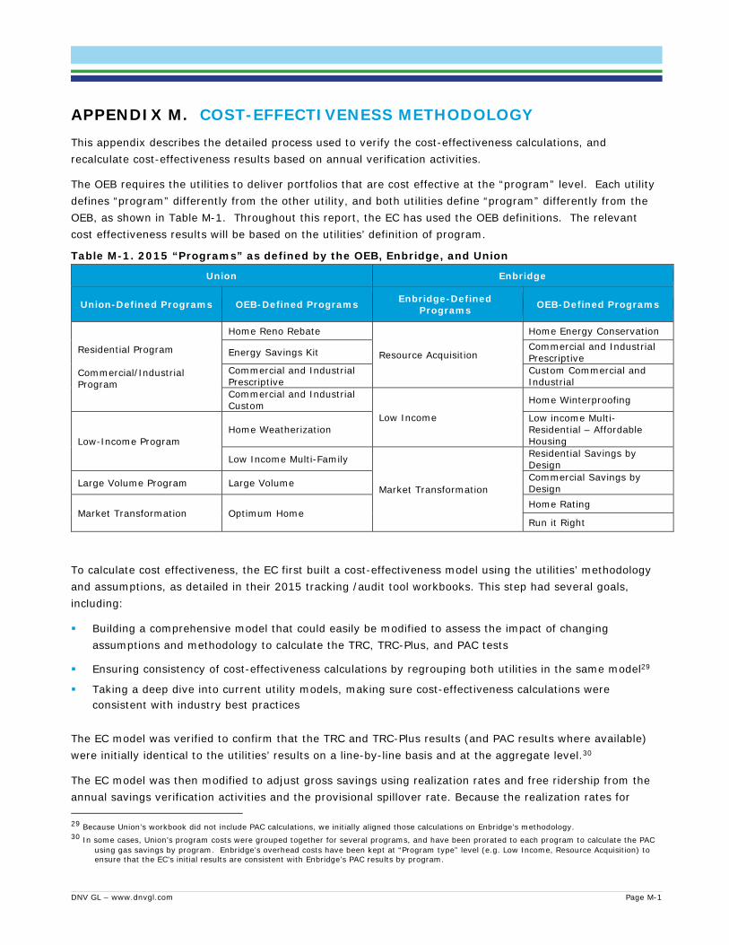
DNV GL – www.dnvgl.com Page M-1
APPENDIX M. COST-EFFECTIVENESS METHODOLOGY This appendix describes the detailed process used to verify the cost-effectiveness calculations, and recalculate cost-effectiveness results based on annual verification activities.
The OEB requires the utilities to deliver portfolios that are cost effective at the “program” level. Each utility defines “program” differently from the other utility, and both utilities define “program” differently from the OEB, as shown in Table M-1. Throughout this report, the EC has used the OEB definitions. The relevant cost effectiveness results will be based on the utilities’ definition of program.
Table M-1. 2015 “Programs” as defined by the OEB, Enbridge, and Union
Union Enbridge
Union-Defined Programs OEB-Defined Programs Enbridge-Defined Programs OEB-Defined Programs
Residential Program Commercial/Industrial Program
Home Reno Rebate
Resource Acquisition
Home Energy Conservation
Energy Savings Kit Commercial and Industrial Prescriptive
Commercial and Industrial Prescriptive
Custom Commercial and Industrial
Commercial and Industrial Custom
Low Income
Home Winterproofing
Low-Income Program Home Weatherization
Low income Multi-Residential – Affordable Housing
Low Income Multi-Family
Market Transformation
Residential Savings by Design
Large Volume Program Large Volume Commercial Savings by Design
Market Transformation Optimum Home Home Rating
Run it Right
To calculate cost effectiveness, the EC first built a cost-effectiveness model using the utilities’ methodology and assumptions, as detailed in their 2015 tracking /audit tool workbooks. This step had several goals, including:
Building a comprehensive model that could easily be modified to assess the impact of changing assumptions and methodology to calculate the TRC, TRC-Plus, and PAC tests
Ensuring consistency of cost-effectiveness calculations by regrouping both utilities in the same model29
Taking a deep dive into current utility models, making sure cost-effectiveness calculations were consistent with industry best practices
The EC model was verified to confirm that the TRC and TRC-Plus results (and PAC results where available) were initially identical to the utilities’ results on a line-by-line basis and at the aggregate level.30
The EC model was then modified to adjust gross savings using realization rates and free ridership from the annual savings verification activities and the provisional spillover rate. Because the realization rates for 29 Because Union’s workbook did not include PAC calculations, we initially aligned those calculations on Enbridge’s methodology. 30 In some cases, Union’s program costs were grouped together for several programs, and have been prorated to each program to calculate the PAC
using gas savings by program. Enbridge’s overhead costs have been kept at “Program type” level (e.g. Low Income, Resource Acquisition) to ensure that the EC’s initial results are consistent with Enbridge’s PAC results by program.

DNV GL – www.dnvgl.com Page M-2
other savings (electricity, water) were generally either not available or much less precise, the gas realization rates were used for all savings.
A series of observations are made in the results section regarding some calculations and assumptions that could be reviewed to better reflect best practices, including the discount rate, the use of a gas benefit adder for the PAC test, and water avoided costs. The impacts of alternative approaches to cost-effectiveness calculations have been calculated using the model with verified savings (i.e., after applying the realization rates and net-to-gross ratios).
Results Table M-2 and Table M-3 show summary results for Union the TRC, TRC-Plus, and PAC tests, including the cost-benefit ratio and the net present value. Table M-4 and Table M-5 show the same information for Enbridge. While there is a general drop in cost-effectiveness results following the verification of savings, almost all OEB-defined programs still pass the cost-effectiveness threshold for both the TRC-Plus and the PAC tests. The only exceptions are the Home Reno Rebate program31 and the RunitRight32 program, shown in tables at the end of this section. In both cases, those programs were not cost-effective when using utility draft reported savings, before any verification-related adjustment. There are additional tables located at the end of this section with more detailed results. When using the utility definition of savings, all programs pass the threshold.
Table M-2. Union summary of cost-effectiveness ratio results
Scorecard
Draft using Utility-Reported Savings* Final Verified Ratio
TRC TRC-Plus** PAC** TRC TRC-Plus PAC
Residential Resource Acquisition 1.2 3.0 8.0
1.0 1.2 2.3
Commercial and Industrial Resource Acquisition 2.9 3.3 3.8 12.0
Low Income 1.0 1.1 0.9 1.3 1.4 1.1
Large Volume 4.7 5.4 26.3 6.0 6.9 10.2
Total Portfolio 2.9 3.3 8.1 2.9 3.3 6.8 * The utility-reported values reflect the savings presented in the utility’s tracking workbook, not in the draft 2015 report. The utility changed the
energy savings values for some projects after submitting the 2015 report but before delivering the data for evaluation, resulting in a small change. **These values were calculated using the utility-reported draft savings results. Union only reported TRC in its filings for 2015.
Table M-3. Union summary of cost-effectiveness net present value results
Scorecard
Draft Net Present Value (M$) using Utility-Reported Savings*
Final Verified Net Present Value (M$)
TRC TRC-Plus** PAC** TRC TRC-Plus PAC
Residential Resource Acquisition 96.7 120.4 117.9
0.4 2.6 6.8
Commercial and Industrial Resource Acquisition 105.4 128.0 124.7
Low Income (0.02) 1.0 (1.1) 1.7 3.1 0.6
Large Volume 70.2 83.6 81.1 27.6 32.6 29.4
Total Portfolio 166.9 205.1 197.9 135.2 166.3 161.5 * The utility-reported values reflect the savings presented in the utility’s tracking workbook, not in the draft 2015 report. The utility changed the
energy savings values for some projects after submitting the 2015 report but before delivering the data for evaluation, resulting in a small change. **These values were calculated using the utility-reported draft savings results. Union only reported TRC in its filings for 2015.
31 The Home Reno Rebate program is not required to be cost effective; only the utility-defined Residential program must be cost effective. 32 The RunitRight program is not required to be cost effective; only the utility-defined Resource Acquisition program must be cost effective.

DNV GL – www.dnvgl.com Page M-3
Table M-4. Enbridge summary of cost-effectiveness ratio results
Scorecard Draft using Utility-Reported Savings* Final Verified Ratio
TRC** TRC-Plus PAC TRC TRC-Plus PAC
Resource Acquisition 3.3 3.8 6.0 2.3 2.7 2.7
Low Income 2.1 2.5 2.5 1.6 1.9 1.7
Total Portfolio 3.1 3.6 5.2 2.2 2.5 2.5 * The utility-reported values reflect the savings presented in the utility’s tracking workbook, not in the draft 2015 report. The utility changed the
energy savings values for some projects after submitting the 2015 report but before delivering the data for evaluation, resulting in a small change. **These values were calculated using the utility-reported draft savings results. Enbridge only reported TRC-Plus and PAC in its filings for 2015.
Table M-5. Enbridge summary of cost-effectiveness net present value results
Scorecard Draft Net Present Value (M$) using
Utility-Reported Savings* Final Verified Net Present Value (M$)
TRC** TRC-Plus PAC TRC TRC-Plus PAC
Resource Acquisition 123.2 149.7 120.4 49.9 61.5 40.7
Low Income 9.2 11.8 10.7 5.0 7.0 5.2
Total Portfolio 132.4 161.6 131.1 54.9 68.5 45.9 * The utility-reported values reflect the savings presented in the utility’s tracking workbook, not in the draft 2015 report. The utility changed the
energy savings values for some projects after submitting the 2015 report but before delivering the data for evaluation, resulting in a small change. **These values were calculated using the utility-reported draft savings results. Enbridge only reported TRC-Plus and PAC in its filings for 2015.
As very low net-to-gross factors were applied to the Large Volume and C&I (Enbridge) custom sectors, the TRC, TRC-Plus, and PAC net values for these sectors dropped significantly.
It is interesting to note that because both savings and costs are affected by the net-to-gross factor, the impact on the TRC and TRC-Plus ratios is far less significant. In addition, a high realization rate (135%) was applied to Union’s Large Volume savings, resulting in an increase of the TRC-Plus ratio, even with a net-to-gross factor of only 12%.
Cost-effectiveness framework Enbridge and Union use divergent cost-effectiveness frameworks to calculate their 2015 results:
Non-energy benefit (NEB) adder: Enbridge uses a 15% NEB adder for both the TRC and the PAC, while Union does not include the adder in their TRC calculations.33
Discount rate: Union uses its weighted average cost of capital (WACC) to discount future values, while Enbridge uses a real discount rate of 4%.
It should also be noted that Enbridge applies a real discount rate to streams of current values. Enbridge notes in the cost-effectiveness workbook provided to the EC that “the Board is of the view that the gas utilities should use a discount rate (real) of 4% when screening prospective DSM programs to determine if they are cost effective for consideration as part of the new 2015 to 2020 multi-year DSM plan. This discount rate is consistent with that used in the electricity Conservation First framework ensuring that all possible energy conservation programs are screened in a consistent manner.”
The Independent Electricity System Operator’s (IESO) Conservation and Demand Management (CDM) Energy Efficiency Cost Effectiveness Guide34 confirms the 4% discount rate in its Appendix A, but states
33 Union’s workbook did not include PAC results. WE calculated the PAC for Union using no NEB adder. 34 March 2015. Conservation and Demand Management Energy Efficiency Cost Effectiveness Guide. Independent Electricity System Operator (IESO).

DNV GL – www.dnvgl.com Page M-4
however that “when performing a cost-effectiveness assessment, the discount rate should be applied to “real” (inflation-adjusted) streams of benefits and costs.” (p.21)
It is the EC’s opinion that a real discount rate should indeed be used only on real streams of benefits and costs. When working with streams of current (nominal) values, a nominal discount rate should instead be used.
Finally, the use of a NEB adder for the PAC test is questionable. The 15% adder accounts for the non-energy benefits associated with DSM programs, such as environmental, economic, and social benefits.35 While DSM programs (mostly those aimed at low income customers) may produce some NEBs at the utility level, such as reduced arrearages, bad debt, and disconnects, the bulk of NEBs are usually at the societal level (reduced GHG and other pollutants) and the participant level (increase comfort, health and safety, etc.), both of which are outside the scope of the PAC test.
The EC did not find any clear indication in OEB decisions or other documentation that the adder should be applied to the PAC. The following excerpt seems to suggest that it should indeed be applied only to the TRC:36
On October 23, 2014, the Minister of Energy amended his Conservation First directive to the OPA and made it mandatory that electricity distributor CDM programs are screened using the TRC test and “include a 15% adder to account for the non-energy benefits associated with the electricity CDM programs, such as environmental, economic, and social benefits.” To effectively align natural gas DSM programs with electricity CDM programs and take into consideration government objectives outlined in the Conservation Directive to the OPA, the Board has concluded that the same approach should be used for screening DSM programs.
The Board will adopt an enhanced TRC test, or the “TRC-Plus” test, which the gas utilities should use to screen all potential DSM programs when developing their multi-year DSM plans. The gas utilities should directly apply a 15% non-energy benefit adder to the benefit side of the TRC test calculation.
The EC team noted that water avoided costs are based on water rates. This has been confirmed by Union: “Water avoided costs are based on average water rates from 17 municipalities across Union’s service territory. This information was used as a proxy to avoided water costs. Avoided water costs and the method of estimating them were filed in Union’s Board-approved 2015-2020 plan.” (Union’s response to EC’s questions on 2015 avoided costs.)
As is the case for gas and electricity, water avoided costs should only include the marginal impact from reduced consumption. Fixed costs (which, in our experience, can represent about 75% to 80% of water costs) must be excluded. On the other hand, water rates are often predominantly or exclusively variable,37 notably to promote conservation, and are thus a bad proxy of avoided costs.
35 2015-2020 Natural Gas Framework (EB-2014-0134), p. 33 36 2015-2020 Natural Gas Framework (EB-2014-0134). Ontario Energy Board, p. 33. In addition, IESO’s March 2015 Conservation and Demand
Management Energy Efficiency Cost Effectiveness Guide clearly states that the adder is to be used only with the TRC. (pp. 31, 32) 37 The City of Toronto, for example, uses a completely variable rate structure.

DNV GL – www.dnvgl.com Page M-5
To simulate the impact of a reduction of water avoided costs, the EC reduced water avoided costs provided by the utilities by 75%. The impact on the TRC-Plus test is slight but not negligible. There is no impact on the PAC, as only gas avoided costs are included in this second test.
To produce results that are more comparable between the two gas utilities, and more consistent with DSM cost-effectiveness best practices, the EC modified results as follows:
Including a 15% NEB adder in Union’s avoided costs for the calculation of the TRC-Plus
Removing the 15% NEB adder for PAC calculations
Using a 4% real discount rate (since both utilities use streams of benefits expressed in nominal dollars, the real rate was converted to a nominal rate of 5.74% using Union’s inflation factor of 1.68%)
Adjusting the water savings benefits to better reflect real avoided costs
With this new set of assumptions, Union’s cost-effectiveness results are increased, while Enbridge’s are decreased. All sectors and portfolios remain cost-effective for both the TRC-Plus and the PAC.
Recommendations This analysis has shown the robustness of DSM results, as cost-effectiveness is generally maintained through the adjustment of claimed savings, net-to-gross factors, discount rates, and water avoided costs.
The EC has the following recommendations results from the cost-effectiveness analysis:
Allocate “sector”-level administrative cost and overhead to each individual program and report program-level cost-effectiveness results. Explicit allocation of general administration and evaluation costs will allow for easier cost-effectiveness calculations at the program level.
Use a consistent real discount rate of 4% for both Enbridge and Union when using “real” (inflation-adjusted) streams of benefits and costs.
Explore the possibility of better defining water avoided costs.
Work towards a better uniformity of cost-effectiveness methods and assumptions between the two gas utilities. There is always a balance to be found between uniform methods and the need to account for the specific situation of each utility. The EC found, however, major discrepancies that could be reduced, such as the discount rate, the use of an NEB adder, the format of reporting results, and the allocation of administration and overhead costs by program.

DNV GL – www.dnvgl.com Page M-6
Table M-6. Union Low Income TRC results
Program Annual net savings (m3)
Measure Incremental
Costs TRC Benefits TRC Costs
(equipment) TRC Value
(equipment) TRC Ratio
(equipment) Program
Admin Costs TRC Ratio (program)
Utility-Reported Draft Results
LI Multi-Family Custom 261,801 1,977,229 577,341 1,977,229 (1,399,888) 0.29 122,815 0.27
LI Multi-Family Prescriptive 589,561 456,435 1,693,096 456,435 1,236,660 3.71 276,572 2.31
Home Weatherization Program 1,341,913 3,453,109 4,927,199 3,453,109 1,474,090 1.43 629,450 1.21
LI Multi-Family Custom - Contrax 57,832 187,055 140,562 187,055 46,493 0.75 27,130 0.66
Utility-Reported Draft Total 2,251,107 6,073,828 7,338,197 6,073,828 1,264,368 1.21 1,055,967 1.03
Final Verified Results
LI Multi-Family Custom 261,801 1,977,229 676,896 1,977,229 (1,300,333) 0.34 122,815 0.32
LI Multi-Family Prescriptive 589,561 456,435 1,997,439 456,435 1,541,004 4.38 276,572 2.72
Home Weatherization Program 1,341,780 3,453,109 6,036,386 3,453,109 2,583,278 1.75 629,450 1.48
LI Multi-Family Custom - Contrax 57,832 187,055 166,626 187,055 (20,429) 0.89 27,130 0.78
Final Verified Total 2,250,974 6,073,828 8,877,348 6,073,828 2,803,520 1.46 1,055,967 1.25

DNV GL – www.dnvgl.com Page M-7
Table M-7. Union Resource Acquisition TRC results
Program Annual net
savings (m3)
Measure Incremental
Costs TRC Benefits TRC Costs
(equipment) TRC Value
(equipment) TRC Ratio
(equipment)
Program Admin Costs
TRC Ratio (program)
Utility-Reported Draft Results
Prescriptive 9,283,248 93,710,064 27,327,806 9,370,064 17,957,742 2.92 531,898 2.76
Agriculture & Greenhouse-Banner 1,406,652 1,464,459 3,017,406 1,464,459 1,552,947 2.06 80,596 1.95
Agriculture & Greenhouse-Contrax 17,779,246 12,334,170 38,785,681 12,334,170 26,451,511 3.14 1,018,689 2.90
Commercial & Institutional Buildings-Banner 1,324,819 4,310,368 3,695,020 4,310,368 (615,348) 0.09 75,908 0.84
Commercial & Institutional Buildings-Contrax 6,277,602 3,575,446 25,100,079 3,575,446 21,524,633 7.02 359,685 6.38
Industrial-Banner 1,287,371 1,559,799 3,265,762 1,559,799 1,705,963 2.09 73,762 2.00
Industrial-Contrax 15,424,080 11,560,886 38,455,282 11,560,886 26,894,396 3.33 883,746 3.09
Energy Savings Kit 1,644,462 139,175 9,133,806 139,175 8,994,632 65.63 310,472 20.31
Home Reno Rebate 3,254,128 12,866,720 9,071,117 12,866,720 (3,795,603) 0.71 614,375 0.67
Utility-Reported Draft Total 57,681,609 57,181,085 157,851,959 57,181,085 100,670,874 2.76 3,949,131 2.58
Final Verified Results
Prescriptive 9,307,088 9,170,777 31,971,550 9,170,777 22,800,773 3.49 552,470 3.29
Agriculture & Greenhouse-Banner 1,346,544 1,401,880 3,247,121 1,401,880 1,845,240 2.32 79,931 2.19
Agriculture & Greenhouse-Contrax 17,019,510 11,807,111 41,348,724 11,807,111 29,541,614 3.50 1,010,281 3.23
Commercial & Institutional Buildings-Banner 1,268,208 4,126,179 4,036,407 4,126,179 (89,771) 0.98 75,281 0.96
Commercial & Institutional Buildings-Contrax 6,009,349 3,422,661 27,091,413 3,422,661 23,668,752 7.92 356,716 7.17
Industrial-Banner 1,232,360 1,493,146 3,491,739 1,493,146 1,998,593 2.34 73,153 2.23
Industrial-Contrax 14,764,984 11,066,870 39,698,891 11,066,870 28,632,021 3.59 876,452 3.32
Energy Savings Kit 1,666,803 151,348 3,969,508 151,348 3,818,160 26.23 313,261 8.54
Home Reno Rebate 3,254,128 12,866,720 10,414,786 12,866,720 (2,451,934) 0.81 611,586 0.77
Final Verified Total 55,868,974 55,506,693 165,270,139 55,506,693 109,763,446 2.98 3,949,131 2.78

DNV GL – www.dnvgl.com Page M-8
Table M-8. Union Large Volume TRC results
Program Annual net savings (m3)
Measure Incremental
Costs TRC Benefits TRC Costs
(equipment) TRC Value
(equipment) TRC Ratio
(equipment) Program
Admin Costs TRC Ratio (program)
Utility-Reported Draft Results
Large Industrial-T1 5,743,536 2,813,262 13,175,552 2,813,262 10,362,290 4.68 115,020 4.50
Large Industrial-T2 38,382,453 13,967,830 69,505,342 13,967,830 55,537,512 4.98 768,645 4.72
Large Industrial-R100 5,131,627 1,305,055 6,628,785 1,305,055 5,323,730 5.08 102,766 4.71
Utility-Reported Draft Total 49,257,616 18,086,146 89,309,678 18,086,146 71,223,532 4.94 986,431 4.68
Final Verified Results
Large Industrial-T1 1,445,698 709,008 4,737,064 709,008 4,028,056 6.68 115,810 5.74
Large Industrial-T2 9,598,272 3,540,164 26,209,242 3,540,164 22,669,079 7.40 768,884 6.08
Large Industrial-R100 1,270,020 322,986 2,236,874 322,986 1,913,888 6.93 101,737 5.27
Final Verified Total 12,313,990 4,572,158 33,183,180 4,572,158 28,611,022 7.26 986,431 5.97
Table M-9. Enbridge overall TRC results
Program Annual net savings (m3)
Measure Incremental
Costs TRC Benefits Program
Costs Overhead TRC Costs TRC Value TRC Ratio
Final Verified Results
Resource Acquisition 28,252,391 23,583,421 77,396,495 3,912,353 5,639,080 33,134,854 49,900,721 2.34
Low Income 4,537,136 6,471,539 13,167,120 1,033,006 617,349 8,121,894 5,045,227 1.62
Table M-10. Enbridge Residential TRC results
Program Annual net savings (m3)
Measure Incremental
Costs TRC Benefits Program Costs TRC Costs TRC Value TRC Ratio
Final Verified Results
Home Energy Conservation 6,762,791 7,790,602 17,154,904 1,021,867 8,812,469 8,342,435 1.95

DNV GL – www.dnvgl.com Page M-9
Table M-11. Enbridge Commercial TRC results
Program Annual net savings (m3)
Measure Incremental
Costs TRC Benefits Program Costs TRC Costs TRC Value TRC Ratio
Final Verified Results
Commercial Prescriptive 5,594,473 3,521,340 17,386,332 - 3,521,340 13,864,992 4.94
Commercial Custom 4,519,626 4,178,176 11,459,659 785,017 4,963,192 6,496,466 2.31
Run It Right 286,985 105,031 243,445 1,471,376 1,576,407 (1,332,963) 0.15
Multi-Residential 2,375,972 2,053,398 7,034,099 41,350 2,094,748 4,939,351 3.36
New Construction 884,643 2,664,670 7,599,092 125 2,664,795 4,934,298 2.85
Final Verified Total 13,661,698 12,522,614 43,722,627 2,297,867 14,820,482 28,902,145 2.95
Table M-12. Enbridge Industrial TRC results
Program Annual net savings (m3)
Measure Incremental
Costs TRC Benefits Program Costs TRC Costs TRC Value TRC Ratio
Final Verified Results
Industrial Custom 7,161,652 2,640,877 14,786,259 10,805 2,651,681 12,134,577 5.58
Industrial Prescriptive 469,002 363,269 1,391,453 581,814 945,084 427,467 1.45
Agriculture 197,247 266,058 360,154 - 266,058 94,096 1.35
Final Verified Total 7,827,901 3,270,204 16,537,866 592,619 3,862,823 12,656,140 4.28
Table M-13. Enbridge Low Income TRC results
Program Annual net savings (m3)
Measure Incremental
Costs TRC Benefits Program Costs TRC Costs TRC Value TRC Ratio
Final Verified Results
Low Income Part 9 1,139,959 3,398,252 3,738,931 679,500 4,077,752 (338,821) 0.92
Low Income Part 3 3,397,177 3,073,287 9,428,190 353,506 3,426,793 6,001,396 2.75
Final Verified Total* 4,537,136 6,471,539 13,167,120 1,033,006 7,504,545 5,662,576 1.75
*This total does not include the Low Income overhead amount, which is why the results are different from the Low Income row in Table M-9.

DNV GL – www.dnvgl.com Page M-10
Table M-14. Union Low Income PAC results
Program Annual net savings (m3)
Program-level
Incentives/ Promotion
Program-level general admin. costs
Portfolio Budget PAC Benefits PAC Costs PAC Value PAC Ratio
Utility-Reported Draft Results**
Low Income 2,251,107 6,645,067 1,055,967 804,624 6,618,986 7,701,034 (1,082,048) 0.86
Final Verified Results
Low Income 2,250,974 6,645,067 1,055,967 804,624 8,284,429 7,701,034 583,395 1.08 **These values were calculated using the utility-reported draft savings results. Union only reported TRC in its filings for 2015.
Table M-15. Union Resource Acquisition PAC results
Program Annual net savings (m3)
Program-level
Incentives/ Promotion
Program-level general admin. costs
Portfolio Budget PAC Benefits PAC Costs PAC Value PAC Ratio
Utility-Reported Draft Results**
Commercial Prescriptive 9,283,248 2,831,233 531,898 208,905 25,120,221 3,363,131 21,757,089 7.47
Commercial Custom 7,602,421 977,281 435,592 171,081 17,790,153 1,412,874 16,377,279 12.59
Small Industrial 16,711,451 2,257,424 957,508 376,065 38,912,289 3,214,932 35,697,357 12.10
Agriculture & Greenhouse 19,185,899 2,278,174 1,099,285 431,749 41,358,032 3,377,460 37,980,572 12.25
Residential 4,898,590 4,525,364 924,847 569,452 11,493,323 5,450,211 6,043,112 2.11
Utility-Reported Draft Total 57,681,609 12,869,476 3,949,131 1,757,251 134,674,017 16,818,607 117,855,410 8.01
Final Verified Results
Commercial Prescriptive 9,307,088 2,831,233 552,470 216,985 29,874,992 3,383,704 26,491,289 8.83
Commercial Custom 7,277,557 977,281 431,997 169,668 19,318,893 1,409,278 17,909,615 13.71
Small Industrial 15,997,344 2,257,424 949,605 372,961 42,428,192 3,207,029 39,221,164 13.23
Agriculture & Greenhouse 18,366,054 2,278,174 1,090,212 428,185 44,474,009 3,368,386 41,105,623 13.20
Residential 4,920,932 4,525,364 924,847 569,452 12,254,926 5,450,211 6,804,716 2.25
Final Verified Total 55,868,974 12,869,476 3,949,131 1,757,251 148,351,013 16,818,607 131,532,406 8.82 **These values were calculated using the utility-reported draft savings results. Union only reported TRC in its filings for 2015.

DNV GL – www.dnvgl.com Page M-11
Table M-16. Union Large Volume PAC results
Program Annual net savings (m3)
Program-level
Incentives/ Promotion
Program-level general admin. costs
Portfolio Budget PAC Benefits PAC Costs PAC Value PAC Ratio
Utility-Reported Draft Results**
Large Industrial-T1 5,743,536 477,540 115,020 39,104 11,600,801 592,560 11,008,241 19.58
Large Industrial-T2 38,382,453 1,359,669 768,645 261,318 66,797,160 2,128,314 64,668,846 31.39
Large Industrial-R100 5,131,627 386,076 102,766 34,937 5,918,686 488,842 5,429,844 12.11
Utility-Reported Draft Total 49,257,616 2,223,285 986,431 335,359 84,316,647 3,209,716 81,106,931 26.27
Final Verified Results
Large Industrial-T1 1,445,698 477,540 115,810 39,372 4,512,275 593,350 3,918,925 7.60
Large Industrial-T2 9,598,272 1,359,669 768,884 261,399 25,947,942 2,128,553 23,819,389 12.19
Large Industrial-R100 1,270,020 386,076 101,737 34,588 2,173,247 487,813 1,685,433 4.46
Final Verified Total 12,313,990 2,223,285 986,431 335,359 32,633,463 3,209,716 29,423,747 10.17 **These values were calculated using the utility-reported draft savings results. Union only reported TRC in its filings for 2015.
Table M-17. Enbridge Residential PAC results Program PAC Benefits PAC Costs PAC Value PAC Ratio
Utility-Reported Draft Results
Home Energy Conservation 20,382,468 9,362,295 11,020,173 2.18
Final Verified Results
Home Energy Conservation 15,833,554 9,362,295 6,471,259 1.69

DNV GL – www.dnvgl.com Page M-12
Table M-18. Enbridge Commercial PAC results Program PAC Benefits PAC Costs PAC Value PAC Ratio
Utility-Reported Draft Results
Commercial Prescriptive 18,785,522 759,387 18,026,134 24.74
Commercial Custom 35,425,654 3,006,848 32,418,806 11.78
Run It Right 542,289 1,458,896 (916,607) 0.37
Multi-Residential 22,201,798 1,527,069 20,674,730 14.54
New Construction 13,685,301 43,749 13,641,552 312.81
Utility-Reported Draft Total 906,640,564 6,795,949 83,844,615 13.34
Final Verified Results
Commercial Prescriptive 13,694,444 759,387 12,935,057 18.03
Commercial Custom 9,525,149 3,006,848 6,518,301 3.17
Run It Right 243,445 1,458,896 (1,215,451) 0.17
Multi-Residential 6,396,804 1,527,069 4,869,735 4.19
New Construction 2,659,747 43,749 2,615,997 60.79
Final Verified Total 32,519,589 6,795,949 25,723,639 4.79
Table M-19. Enbridge Industrial PAC results Program PAC Benefits PAC Costs PAC Value PAC Ratio
Utility-Reported Draft Results
Industrial Custom 31,091,685 2,032,054 29,059,631 15.30
Industrial Prescriptive 1,385,792 27,150 1,358,642 51.04
Agriculture 894,031 107,502 786,529 8.32
Utility-Reported Draft Total 33,371,509 2,166,706 31,204,802 15.40
Final Verified Results
Industrial Custom 14,735,667 2,032,054 12,703,614 7.25
Industrial Prescriptive 1,213,351 27,150 1,186,201 44.69
Agriculture 360,154 107,502 252,652 3.35
Final Verified Total 16,309,173 2,166,706 14,142,466 7.53

DNV GL – www.dnvgl.com Page M-13
Table M-20. Enbridge Low Income PAC results Program PAC Benefits PAC Costs PAC Value PAC Ratio
Utility-Reported Draft Results
Low Income Part 9 5,178,114 4,444,616 733,498 1.17
Low Income Part 3 12,691,944 2,111,746 10,580,198 6.01
Utility-Reported Draft Total 178,700,528 6,556,362 11,313,696 2.73
Final Verified Results
Low Income Part 9 3,721,339 4,444,616 (723,277) 0.84
Low Income Part 3 8,677,326 2,111,746 6,565,580 4.11
Final Verified Total* 12,398,665 6,556,362 5,842,303, 1.89
*This total does not include the Low Income overhead amount, which is why the results are different from the Low Income row in Table M-21.
Table M-21. Enbridge overall PAC results Program PAC Benefits PAC Costs PAC Value PAC Ratio
Utility-Reported Draft Results
Resource Acquisition 144,394,541 23,964,031 120,430,511 6.03
Low Income 17,870,058 7,173,711 10,696,347 2.49
Utility-Reported Draft Total 162,264,599 31,137,742 131,126,858 5.21
Final Verified Results
Resource Acquisition 64,662,316 23,964,031 40,698,285 2.70
Low Income 12,398,665 7,173,711 5,224,954 1.73
Final Verified Total 77,060,981 31,137,742 45,923,239 2.47

DNV GL – www.dnvgl.com Page M-14
Table M-22. Union Low Income TRC-Plus results
Program Annual net savings (m3)
Measure Incremental
Costs
TRC-Plus Benefits
TRC Costs (equipment)
TRC Value (equipment)
TRC Ratio (equipment)
Program Admin Costs
TRC Ratio (program)
Final Verified Results
LI Multi-Family Custom 261,801 1,977,229 778,431 1,977,229 (1,198,798) 0.39 122,815 0.37
LI Multi-Family Prescriptive 589,561 456, 435 2,297,055 456,435 1,840,620 5.03 276,572 3.13
Home Weatherization Program 1,341,780 3,453,109 6,941,844 3,453,109 3,488,736 2.01 629,450 1.70
LI Multi-Family Custom - Contrax 57,832 187,055 191,620 187,055 4,565 1.02 27,130 0.89
Final Verified Total 2,250,974 6,073,828 10,208,950 6,073,854 4,135,122 1.68 1,055,967 1.43
Table M-23. Union Resource Acquisition TRC-Plus results
Program Annual net
savings (m3)
Measure Incremental
Costs
TRC-Plus Benefits
TRC Costs (equipment)
TRC Value (equipment)
TRC Ratio (equipment)
Program Admin Costs
TRC Ratio (program)
Final Verified Results
Prescriptive 9,307,088 9,170,777 36,767,282 9,170,777 27,596,505 4.01 552,470 3.78
Agriculture & Greenhouse-Banner 1,346,544 1,401,880 3,734,189 1,401,880 2,332,308 2.66 79,931 2.52
Agriculture & Greenhouse-Contrax 17,019,510 11,807,111 47,551,033 11,807,111 35,743,922 4.03 1,010,281 3.71
Commercial & Institutional Buildings-Banner 1,268,208 4,126,179 4,641,868 4,126,179 515,690 1.12 75,281 1.10
Commercial & Institutional Buildings-Contrax 6,009,349 3,422,661 31,155,125 3,422,661 27,732,464 9.1 356,716 8.24
Industrial-Banner 1,232,360 1,493,146 4,015,500 1,493,146 2,522,354 2.69 73,153 2.56
Industrial-Contrax 14,764,984 11,066,870 45,653,724 11,066,870 34,586,854 4.13 876,452 3.82
Energy Savings Kit 1,666,803 151,348 4,564,935 151,348 4,413,586 30.16 313,261 9.83
Home Reno Rebate 3,254,128 12,866,720 11,977,004 12,866,720 (889,716) 0.93 611,586 0.89
Final Verified Total 55,868,974 55,506,693 190,060,660 55,506,693 134,553,967 3.42 3,949,131 3.20

DNV GL – www.dnvgl.com Page M-15
Table M-24. Union Large Volume TRC-Plus results
Program Annual net savings (m3)
Measure Incremental
Costs
TRC-Plus Benefits
TRC Costs (equipment)
TRC Value (equipment)
TRC Ratio (equipment)
Program Admin Costs
TRC Ratio (program)
Final Verified Results
Large Industrial-T1 1,445,698 709,008 5,447,623 709,008 4,738,615 7.68 115,810 6.60
Large Industrial-T2 9,598,272 3,540,164 30,140,629 3,540,164 26,600,465 8.51 768,884 6.99
Large Industrial-R100 1,270,020 322,986 2,572,405 322,986 2,249,419 7.96 101,737 6.06
Final Verified Total 12,313,990 4,572,158 38,160,657 4,572,158 33,588,499 8.35 986,431 6.87
Table M-25. Enbridge overall TRC-Plus results
Scorecard Annual net savings (m3)
Measure Incremental
Costs
TRC-Plus Benefits
Program Costs Overhead TRC Costs TRC Value TRC Ratio
Final Verified Results
Resource Acquisition 28,252,391 23,583,391 89,005,969 3,912,353 5,639,080 33,134,854 61,510,195 2.69
Low Income 4,537,136 6,471,539 15,142,189 1,033,006 617,349 8,121,894 7,020,295 1.86
Table M-26. Enbridge Residential TRC-Plus results
Program Annual net savings (m3)
Measure Incremental
Costs
TRC-Plus Benefits Program Costs TRC Costs TRC Value TRC Ratio
Utility-Reported Draft Results
Home Energy Conservation 6,762,791 7,790,602 22,077,884 1,021,867 8,812,469 132,654,158 2.51
Final Verified Results
Home Energy Conservation 6,762,791 7,790,602 19,728,139 1,021,867 8,812,469 10,915,671 2.24

DNV GL – www.dnvgl.com Page M-16
Table M-27. Enbridge Commercial TRC-Plus results
Program Annual net savings (m3)
Measure Incremental
Costs
TRC-Plus Benefits Program Costs TRC Costs TRC Value TRC Ratio
Utility-Reported Draft Results
Commercial Prescriptive 5,750,534 3,640,863 30,989,923 - 3,640,863 27,349,060 8.51
Commercial Custom 12,326,277 11,395,046 42,631,687 785,017 12,180,063 30,451,624 3.50
Run It Right 536,821 196,467 542,289 1,471,376 1,667,843 (1,125,554) 0.33
Multi-Residential 5,890,850 5,091,080 24,316,449 41,350 5,132,430 19,184,019 4.74
New Construction 3,027,916 9,120,516 39,043,342 125 9,120,641 29,922,701 4.28
Utility-Reported Draft Total 27,532,399 29,443,972 137,523,689 2,297,867 31,741,839 105,781,850 4.33
Final Verified Results
Commercial Prescriptive 5,594,473 3,521,340 19,994,282 - 3,521,340 16,472,942 5.68
Commercial Custom 4,519,626 4,178,176 13,178,607 785,017 4,963,192 8,215,415 2.66
Run It Right 286,985 105,031 279,961 1,471,376 1,576,407 (1,296,446) 0.18
Multi-Residential 2,375,972 2,053,398 8,089,214 41,350 2,094,748 5,994,466 3.86
New Construction 884,643 2,664,670 8,738,956 125 2,664,795 6,074,161 3.28
Final Verified Total 13,661,698 12,522,614 50,281,021 2,297,867 14,820,482 35,460,539 3.39
Table M-28. Enbridge Industrial TRC-Plus results
Program Annual net savings (m3)
Measure Incremental
Costs
TRC-Plus Benefits Program Costs TRC Costs TRC Value TRC Ratio
Utility-Reported Draft Results
Industrial Custom 11,097,622 4,092,276 33,723,828 10,805 4,103,080 29,620,748 8.22
Industrial Prescriptive 398,824 304,562 1,553,550 581,814 886,376 667,174 1.75
Agriculture 366,783 494,737 894,031 - 494,737 399,294 1.81
Utility-Reported Draft Total 11,863,229 4,891,575 36,171,410 592,619 5,484,194 30,687,216 6.60
Final Verified Results
Industrial Custom 7,161,652 2,640,877 17,004,197 10,805 2,651,681 14,352,516 6.41
Industrial Prescriptive 469,002 363,269 1,578,433 581,814 945,084 633,350 1.67
Agriculture 197,247 266,058 414,177 - 266,058 148,119 1.56
Final Verified Total 7,827,902 3,270,204 18,996,808 592,619 3,862,823 15,133,985 4.92

DNV GL – www.dnvgl.com Page M-17
Table M-29. Enbridge Low Income TRC-Plus results
Program Annual net savings (m3)
Measure Incremental
Costs
TRC-Plus Benefits Program Costs TRC Costs TRC Value TRC Ratio
Utility-Reported Draft Results
Low Income Part 9 1,139,959 3,398,252 5,253,138 679,500 4,077,752 1,175,386 1.29
Low Income Part 3 3,397,177 3,073,287 14,695,099 353,506 3,426,793 11,268,305 4.29
Utility-Reported Draft Total 4,537,136 6,471,539 19,948,237 1,033,006 7,504,545 12,443,691 2.66
Final Verified Results
Low Income Part 9 1,139,959 3,398,252 4,299,771 679,500 4,077,752 222,019 1.05
Low Income Part 3 3,397,177 3,073,287 10,842,418 353,506 3,426,793 7,415,625 3.16
Final Verified Total* 4,537,136 6,471,539 15,142,189 1,033,006 7,504,545 7,637,644 2.02
*This total does not include the Low Income overhead amount, which is why the results are different from the Low Income row in Table M-25.

DNV GL – www.dnvgl.com Page N-1
APPENDIX N. SPILLOVER ESTIMATE This appendix describes the source of the estimated value used for spillover and how it was added to the free ridership estimate to produce the NTG ratio for custom projects.38
A spillover study is currently being conducted on Ontario gas utilities’ custom projects from 2013 and 2014; however, those results are not yet available. The OEB asked the EC to conduct secondary source research to identify an estimate that might reasonably be applied to the Ontario DSM programs as an estimate for the 2015 clearance of accounts. The EC selected a 3.4% spillover rate based on a study in Massachusetts.39 This is the most applicable value for the Ontario DSM programs because:
Massachusetts has a similar climate to Ontario’s major population centers, so it is likely that similar measures are being implemented
The spillover value is specifically for custom gas C&I measures, which is the same program type
The programs in Massachusetts and Ontario are mature and in leading jurisdictions
The Massachusetts study looked at both “like” and “unlike” spillover40
The rate is within the anticipated range of results expected for spillover from custom gas C&I programs, not an extreme outlier
The study is relatively recent, from 2014-15.
The major differences from the Ontario spillover study are as follows:
It only quantifies (provides a savings estimate for) like spillover, not unlike spillover.
The study was conducted on customers who had participated in the program 15-27 months prior, not four or five years ago. This provides for less time since the program measure for spillover to occur.
The spillover estimate was added to the measured free ridership rate from the CPSV/NTG study (APPENDIX H). Table N-1 and Table N-2 show the free ridership, spillover, and NTG adjustment factors.
The NTG adjustment factors were applied to the verified gross savings to produce verified net savings.
38 Spillover is only added to custom projects in C&I and Large Volume, not Low Income. 39 Tetra Tech. “2014-15 Commercial and Industrial Natural Gas Programs Free-ridership and Spillover Study” for National Grid, Eversource, Unitil,
Berkshire Gas, Columbia Gas of MA, and Liberty Utilities. Revised August 10, 2015. 40 Like spillover refers to energy efficient equipment installed by a participant due to program influence that is identical to the equipment they
received through the program. Unlike spillover is installed equipment due to program influence that is different from what they received through the program.

DNV GL – www.dnvgl.com Page N-2
Table N-1. Union free ridership, spillover, and NTG adjustment factors by subset
Program Free Ridership Adjustment† Spillover Addition Net-to-Gross
Adjustment†
C&I Custom Comm & Inst Buildings 44% 3.4% 47%
C&I Custom Ag and Greenhouse 41% 3.4% 44%
C&I Custom Industrial 39% 3.4% 43%
Large Industrial R100 8% 3.4% 12%
Large Industrial T1 9% 3.4% 13%
Large Industrial T2 8% 3.4% 11% †These values are rounded.
Table N-2. Enbridge CPSV and NTG adjustment factors
Program Free Ridership Adjustment† Spillover Addition Net-to-Gross
Adjustment†
Custom Commercial 17% 3.4% 21%
C&I Custom New Construction 18% 3.4% 22%
Custom Multi-family 35% 3.4% 38%
Custom Industrial Ag 28% 3.4% 32%
Custom Industrial 33% 3.4% 36%
RunitRight 50% 3.4% 53% †These values are rounded.

DNV GL – www.dnvgl.com Page O-1
APPENDIX O. FINAL ANNUAL VERIFICATION EM&V PLAN Embedded below is the detailed plan for the 2015 verification. The plan was largely implemented as written; however, there was a large divergence from the original schedule.
Detailed Plan for 2015 Annual Verifica

Natural Gas Demand Side Management - Detailed Plan for 2015 Annual Verification submitted to the Ontario Energy Board
Date: January 13, 2017

DNV GL – www.dnvgl.com 1/13/17 Page i
Table of contents
1 INTRODUCTION ............................................................................................................ 2
2 REPORTED METRICS TO VERIFY ...................................................................................... 3
3 ACTIVITIES .................................................................................................................. 8
4 WHAT INFORMATION IS NECESSARY ............................................................................. 12
5 OUTCOMES AND REVIEW PROCESS ............................................................................... 15
6 SCHEDULE ................................................................................................................. 16

DNV GL – www.dnvgl.com 1/13/17 Page 2
1 INTRODUCTION This document has been prepared for the Ontario Energy Board (OEB) and outlines the detailed plan for conducting the annual verification of Enbridge Gas Distribution Inc.’s (Enbridge) and Union Gas Limited’s (Union) natural gas demand-side management (DSM) programs delivered in 2015. These verifications will be conducted by the Evaluation Contractor (EC) team.
The overall objectives of the evaluations are to:
Provide an independent opinion on whether the Lost Revenue Adjustment Mechanism (LRAM), DSM Variance Account (DSMVA), and DSM Shareholder Incentive (DSMSI) were reasonable, appropriate, and calculated correctly.
Recommend future evaluation research opportunities to enhance the assumptions used to calculate DSMSI and LRAM amounts.
Recommend changes to improve input assumptions, verification procedures, and the overall verification process.
The LRAM, DSMVA, and DSMSI are based on the following metrics:
LRAM: the verified natural gas energy savings (in annual cubic meters) by rate class (rounded to the nearest 1,000 cubic meters) and the cost of the natural gas by rate class for the program year.
DSMVA: the actual money collected, by rate class, for implementing DSM programs during the program year and the actual DSM costs incurred by the programs.
DSMSI: the actual program achievements compared to the scorecard metrics for that program, the weight placed on each metric within each scorecard, and the maximum incentive achievable for that scorecard.
Therefore, the information that must be verified for 2015 includes the program natural gas savings and the program achievements compared to the scorecard metrics. The EC will also review the money collected and spent by the programs but will not conduct a full financial audit of the reported amounts. The OEB may conduct financial audits of the gas utilities DSM spending as it sees fit. The verified savings and program achievements will be used to confirm the LRAM and DSMSI amounts.
The remainder of this document provides the following:
An overview of the 2015 programs and their scorecard metrics A list of the data, documentation, and other information necessary to conduct the verification A list of the activities that will be conducted as part of the verification An accounting of the expected verification outcomes and the process for reviewing those
outcomes A proposed schedule for completing the verification
While some information related to the verification of custom projects (i.e. Custom Project Savings Verification, or CPSV) can be found in this document, it is not considered part of the “annual verification” and the details are located elsewhere.

DNV GL – www.dnvgl.com 1/13/17 Page 3
2 REPORTED METRICS TO VERIFY To verify the LRAM and DSMSI, the EC must verify the reported utility achievements for each scorecard, as well as verify the energy savings achieved by each rate class. Table 2-1 and Table 2-2 show the 2015 targets, weights, and maximum shareholder incentive by scorecard (resource acquisition, large volume, low income, and market transformation) for Union and Enbridge, respectively. It also shows the reported 2015 achievement for each utility. Because some scorecards are a compilation of the achievements of multiple programs, Table 2-3 and Table 2-4 show the scorecard metrics and energy savings achievements by program.

DNV GL – www.dnvgl.com 1/13/17 Page 4
Table 2-1. Union’s Reported 2015 achievement, target, weight, and maximum shareholder incentive by scorecard
Scorecard 2015 Target 2015 Reported
Achievement
% of Target
Weight Maximum Shareholder Incentive (if
150% of target
achieved)
Union
Resource Acquisition 816,561,818 CCM
1,245 deep savings participants
8.88% of commercial whole building natural gas use saved
938,905,035 CCM
2,537 participants
8.24% saved
130%
308%
68%
90%
5%
5%
$5,761,833
Large Volume 206,256,017 Rate 1 CCM
1,029,841,387 Rate T2/100 CCM
78,919,835 CCM
499,103,360 CCM
-23%
-3%
60%
40%
$1,862,877
Low Income 26,000,000 single family CCM
17,600,000 multi-family CCM
33,504,841 CCM
16,948,695 CCM
158%
93%
60%
40%
$2,810,129
Market Transformation
30% of homes built by participating builders were 20% more efficient than OBC
50% of homes 306% 100% $566,721
TOTAL $11,001,560

DNV GL – www.dnvgl.com 1/13/17 Page 5
Table 2-2. Enbridge’s Reported 2015 achievement, target, weight, and maximum shareholder incentive by scorecard
Scorecard 2015 Target 2015 Reported Achievement
% of Target
Weight Maximum Shareholder Incentive (if
150% of target
achieved)
Enbridge
Resource Acquisition 1,011,900,000 CCM
762 deep savings participants
767,627,826 CCM
5,646 participants
52%
1385%
92%
8%
$6,482,744
Low Income 24,100,000 single family CCM
68,700,000 multi-family CCM
40% of Part 3 participants enrolled
28,343,978 CCM
69,226,782 CCM
65% enrolled
135%
102%
224%
50%
45%
5%
$2,495,721
Residential Savings by Design (Market Transformation)
18 Builders enrolled
1,111 homes built 20% more efficient than OBC
19 Builders enrolled
1,987 of homes
113%
258%
20%
13%
$1,076,493
Commercial Savings by Design (Market Transformation)
18 New developments enrolled 24 developments enrolled
150% 33% $418,269
Home Labelling (Market Transformation)
5,000 Realtor commitments
4,500 Ratings performed
41,650 Realtor commitments
336 Ratings performed
466%
7%
17%
17%
$616,397
TOTAL $11,089,624
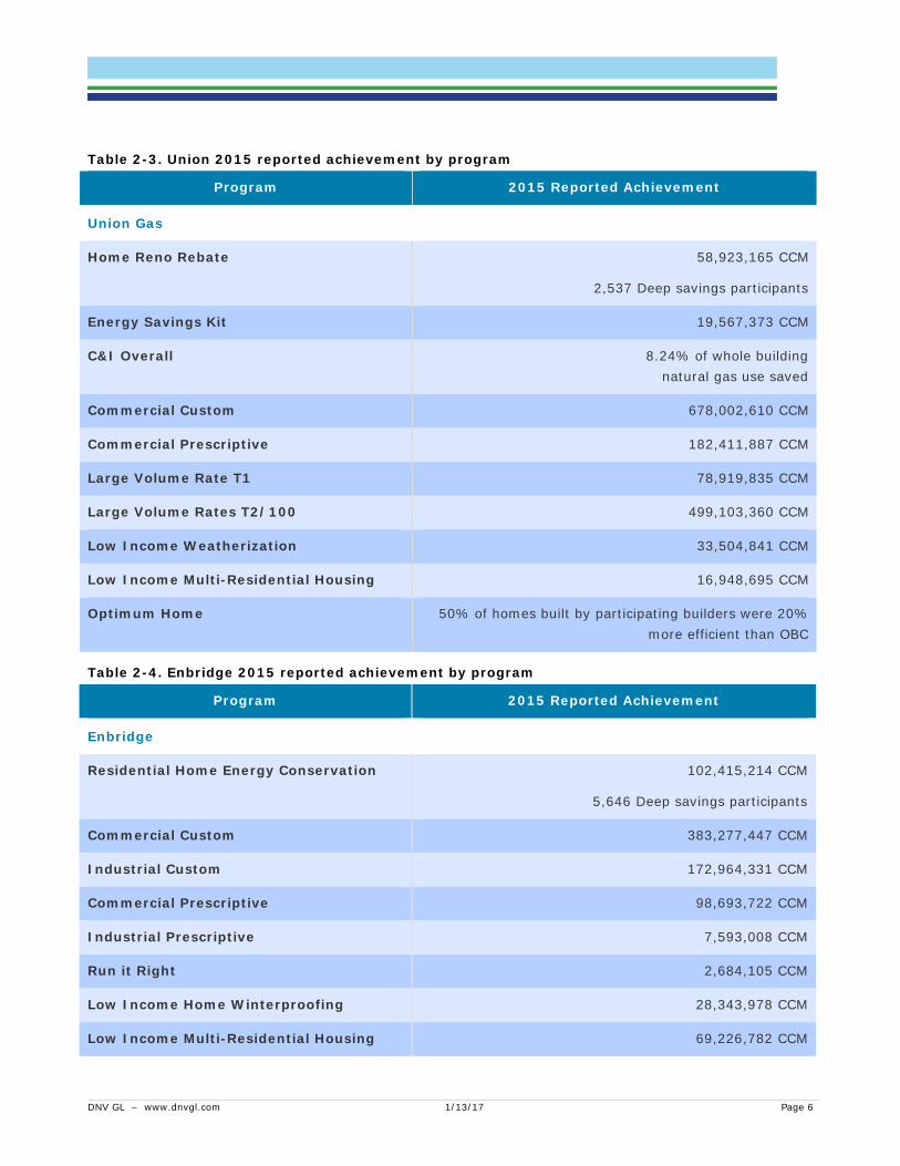
DNV GL – www.dnvgl.com 1/13/17 Page 6
Table 2-3. Union 2015 reported achievement by program
Program 2015 Reported Achievement
Union Gas
Home Reno Rebate 58,923,165 CCM
2,537 Deep savings participants
Energy Savings Kit 19,567,373 CCM
C&I Overall 8.24% of whole building natural gas use saved
Commercial Custom 678,002,610 CCM
Commercial Prescriptive 182,411,887 CCM
Large Volume Rate T1 78,919,835 CCM
Large Volume Rates T2/100 499,103,360 CCM
Low Income Weatherization 33,504,841 CCM
Low Income Multi-Residential Housing 16,948,695 CCM
Optimum Home 50% of homes built by participating builders were 20% more efficient than OBC
Table 2-4. Enbridge 2015 reported achievement by program
Program 2015 Reported Achievement
Enbridge
Residential Home Energy Conservation 102,415,214 CCM
5,646 Deep savings participants
Commercial Custom 383,277,447 CCM
Industrial Custom 172,964,331 CCM
Commercial Prescriptive 98,693,722 CCM
Industrial Prescriptive 7,593,008 CCM
Run it Right 2,684,105 CCM
Low Income Home Winterproofing 28,343,978 CCM
Low Income Multi-Residential Housing 69,226,782 CCM

DNV GL – www.dnvgl.com 1/13/17 Page 7
Program 2015 Reported Achievement
65% of Part 3 participants enrolled
Residential Savings by Design 19 Builders enrolled
1,987 homes built 20% more efficient than OBC
Commercial Savings by Design 24 New developments enrolled
Home Labelling 41,650 Realtor commitments
336 Ratings performed

DNV GL – www.dnvgl.com 1/13/17 Page 8
3 ACTIVITIES To verify the information reported in section 2, the EC will conduct the activities outlined in Table 3-1 and Table 3-2. To prepare for the program-specific activities, the EC will request tracking data and documentation, specified in section 4. For all programs, the EC will first review the reported savings and metrics from the tracking data and compare them to the summarized information in the gas utilities’ annual report to ensure consistency. We will also recreate the reported DSMVA, LRAM, and DSMSI values using the reported savings and scorecard achievements to confirm that the calculations were done correctly.
Once the program-specific verifications are completed, the EC will assemble the verified scorecard results and calculate the verified LRAM, DSMVA, and DSMSI results as necessary. We will also document any recommendations that may improve the annual verification process going forward.

DNV GL – www.dnvgl.com 1/13/17 Page 9
Table 3-1. 2015 Annual verification activities for Union, by program
Program Metrics Activity
Union Gas
Home Reno Rebate
Energy Savings Kit
Low Income Weatherization
Low Income Multi-Residential Housing
Natural gas savings (CCM)
Number of deep savings participants
Confirm that the measure-level inputs for prescriptive measures were appropriate and confirm that the savings were calculated correctly for a census (or the full population) of measures.
Verify the number of deep savings participants by reviewing the detailed documentation for a sample of participants.
Apply the results of the CPSV / NTG study, where appropriate.
Commercial Custom Natural gas savings (CCM)
Average percent of whole building energy use saved by the program
Confirm that the necessary factors (such as NTG assumptions) were applied correctly and that recommendations from previous evaluations were adopted.
Apply the results of the CPSV / NTG study.
Collect the annual billing information for a census of participants and compare the verified energy savings to the annual energy use to confirm the percent of whole building natural gas use saved.
Commercial Prescriptive Natural gas savings (CCM)
Average percent of whole building energy use saved by the program
Confirm that the measure-level inputs for prescriptive measures were appropriate and confirm that the savings were calculated correctly for a census of measures.
Collect the annual billing information for a census of participants and compare verified energy savings to the annual energy use to confirm the percent of whole building natural gas use saved.

DNV GL – www.dnvgl.com 1/13/17 Page 10
Program Metrics Activity
Large Volume Natural gas savings (CCM)
Confirm that the necessary factors (such as NTG assumptions) were applied correctly and that recommendations from previous evaluations were adopted.
Apply the results of the CPSV / NTG study.
Optimum Home Percent of homes built by participating builders that are 20% more efficient than OEB
Review the procedure used for determining the scorecard metric to confirm whether it leads to accurate results.

DNV GL – www.dnvgl.com 1/13/17 Page 11
Table 3-2. 2015 Annual verification activities for Enbridge, by program
Program Metrics Activity
Enbridge
Residential Home Energy Conservation
Low Income Home Winterproofing
Low Income Multi-Residential Housing
Natural gas savings (CCM)
Number of deep savings participants
Percent of Part 3 participants enrolled
Confirm that the measure-level inputs for prescriptive measures were appropriate and confirm that the savings were calculated correctly for a census of measures.
Verify the number of deep savings participants by reviewing the detailed documentation for a sample of participants.
Review documentation to confirm the Part 3 participant low income scorecard metric.
Apply the results of the CPSV / NTG study, where appropriate.
Commercial and Industrial Custom Natural gas savings (CCM) Confirm that the necessary factors (such as NTG assumptions) were applied correctly and that recommendations from previous evaluations were adopted.
Apply the results of the CPSV / NTG study.
Commercial and Industrial Prescriptive
Natural gas savings (CCM) Confirm that the measure-level inputs for prescriptive measures were appropriate and confirm that the savings were calculated correctly for a census of measures.
Run it Right Natural gas savings (CCM) Conduct a desk review of a sample of participants to verify the reasonableness of the claimed savings.
Residential Savings by Design
Commercial Savings by Design
Home Labelling
Builders enrolled Number of efficient homes Number of developments Number of realtor commitments Number of ratings performed
Review the procedure used for determining the scorecard metrics to confirm whether it leads to accurate results.

DNV GL – www.dnvgl.com 1/13/17 Page 12
4 WHAT INFORMATION IS NECESSARY DNV GL will request data and documentation in two waves. The first documentation request will address the tracking data for each program, documentation and support for prescriptive savings calculations, assumptions and adjustments (such as NTG assumptions) for custom savings projects, billing data for Union commercial customers, and an explanation for how metrics for market transformation programs are counted and tracked. The second documentation request will be significantly smaller, requesting documentation on a sample of Run it Right and Home Reno Rebate / Residential Home Energy Conservation participants.
The detailed data requested as part of the two documentation requests are shown in Table 4-1. Per the schedule outlined in section 6, the EC will send a formal documentation request for Round 1 on January 6th, with delivery due January 20th. The EC will send a formal documentation request for Round 2 on January 31st at the latest, with delivery due on February 14th.
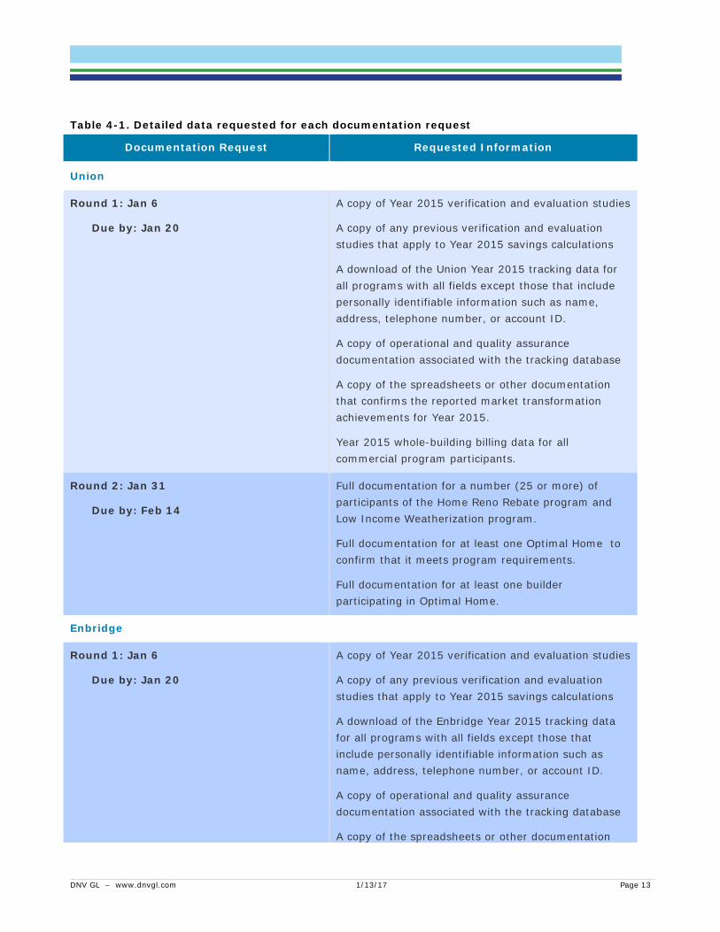
DNV GL – www.dnvgl.com 1/13/17 Page 13
Table 4-1. Detailed data requested for each documentation request
Documentation Request Requested Information
Union
Round 1: Jan 6
Due by: Jan 20
A copy of Year 2015 verification and evaluation studies
A copy of any previous verification and evaluation studies that apply to Year 2015 savings calculations
A download of the Union Year 2015 tracking data for all programs with all fields except those that include personally identifiable information such as name, address, telephone number, or account ID.
A copy of operational and quality assurance documentation associated with the tracking database
A copy of the spreadsheets or other documentation that confirms the reported market transformation achievements for Year 2015.
Year 2015 whole-building billing data for all commercial program participants.
Round 2: Jan 31
Due by: Feb 14
Full documentation for a number (25 or more) of participants of the Home Reno Rebate program and Low Income Weatherization program.
Full documentation for at least one Optimal Home to confirm that it meets program requirements.
Full documentation for at least one builder participating in Optimal Home.
Enbridge
Round 1: Jan 6
Due by: Jan 20
A copy of Year 2015 verification and evaluation studies
A copy of any previous verification and evaluation studies that apply to Year 2015 savings calculations
A download of the Enbridge Year 2015 tracking data for all programs with all fields except those that include personally identifiable information such as name, address, telephone number, or account ID.
A copy of operational and quality assurance documentation associated with the tracking database
A copy of the spreadsheets or other documentation

DNV GL – www.dnvgl.com 1/13/17 Page 14
Documentation Request Requested Information
that confirms the reported market transformation achievements for Year 2015.
Documentation that confirms the Part 3 enrollment percentage
Round 2: Jan 31
Due by: Feb 14
Full documentation for a number (25 or more) of participants of the Home Energy Conservation program and Low Income Weatherization program.
Full documentation for at least one Residential Savings by Design home to confirm that it meets program requirements.
Full documentation for at least one builder participating in Residential Savings by Design.
Full documentation for at least one Commercial Savings by Design development to confirm that it meets program requirements.
Full documentation for at least one builder participating in Commercial Savings by Design.
Full documentation of at least one realtor commitment and subsequent ratings performed for Home Labeling.

DNV GL – www.dnvgl.com 1/13/17 Page 15
5 OUTCOMES AND REVIEW PROCESS The annual verification process will produce verified energy savings and scorecard achievements (by utility, scorecard, and program) for the 2015 program year. It will also produce updated LRAM, DSMVA, and DSMSI amounts that can be used in the clearance of accounts proceedings. The EC will assemble the verification methodology, reported achievements, and verified results into a single report for review and comment by the OEB and Evaluation Advisory Committee (EAC). The EC will also include recommendations for future improvements, high-level results from additional evaluation studies conducted on the 2015 program year data (such as the CPSV / NTG study), and the full reports of those studies in attached appendices. In effect, the annual verification process will produce a report that summarizes all of the recent evaluation and verification studies completed, their outcomes, and how they were applied to the 2015 program year.
At a high level, the verification report will include the following sections:
Executive Summary: This section will summarize the introduction and objective of the document and report on the verified scorecard achievements for the 2015 program year. The Executive Summary will also include the verified LRAM, DSMVA, and DSMSI amounts.
Introduction: This section will introduce the verification study, its objectives, and how the document reports the accomplishments.
Methodology: This section will summarize the evaluation and verification activities undertaken to verify the 2015 program year savings and scorecard metrics. The section will be a high-level summary of the activities and use appendices to provide additional detail.
Results: This section will report on the results of the annual verification and summarize the high-level results of additional evaluation activities. It will also report on the application of those results to the LRAM, DSMVA, and DSMSI calculations and the final outcomes.
Conclusions: This section will summarize the LRAM, DSMVA, and DSMSI final results and summarize any recommendations made throughout the annual verification report, including those made in the additional evaluation reports.
The EC team proposes an unusual review structure to coordinate with the CPSV / NTG study and meet an aggressive March 31, 2016 deadline. We propose to distribute an incomplete draft report that includes all of the necessary verification factors EXCEPT the final results of the CPSV / NTG study on March 10. The next two weeks (until March 24th) would be used for review, comment, and addressing the comments on the annual verification report, minus the CPSV / NTG results. When the CPST / NTG results are finalized, on or just before March 31, they would be incorporated into the annual report, which would be finalized without an additional round of review.
The entire schedule is shown in section 6.

DNV GL – www.dnvgl.com 1/13/17 Page 16
6 SCHEDULE This section outlines the project tasks and schedule for the 2015 annual verification. The schedule is shown in Table 6-1, which lists each verification task and the start and end dates for completing that task. Bolded rows (and green-filled cells) are “super” tasks. The indented, non-bolded (and blue-filled cells) rows are sub-tasks within that super-task.
The schedule is aggressive and designed to limit interference with the CPSV / NTG study as much as possible. It is also designed to produce a final report on March 31st to meet OEB reporting requirements.
Table 6-1. Schedule of deliverables
Task Dec Jan Feb Mar Detailed plan Initial tracking data review 6th 17th
Initial data request 6th Initial data delivery 20th Identify sample for detailed review 31st Documentation request 31st Final documentation delivery 14th
Tracking savings certification 20th 3rd Confirm match with reporting 20th - 27th Assemble assumptions and adjustments 20th - 27th Recreate savings estimates 27th 17th Confirm/verify errors with utilities 17th 3rd
Documentation review Run it Right analysis 15th 3rd Deep savings analysis 27th 3rd Enbridge Part 3 analysis 27th 3rd Market transformation analysis 15th 3rd Union commercial percentage analysis 15th 3rd
Verified results 30th 31st Verify DSMVA, LRAM, DSMSI calculations 30th 10th Assemble tracking and documentation results 17th 10th Produce verified scorecard metrics 17th 10th Apply CPSV / NTG results 31st
Reporting 17th 31st Write recommendations 17th 15th Draft results without CPSV / NTG 10th – 24th Final results with all factors 31st
Project Management
The EC has highlighted the tasks that require utility involvement and the dates of that involvement, in Table 6-2. There are two documentation delivery periods: one for the initial tracking data, and a follow-up period to deliver detailed documentation for a sample of measures from select programs. There are also two

DNV GL – www.dnvgl.com 1/13/17 Page 17
review periods: one for discussing any discrepancies from the tracking savings certification, and one for the overall draft report.
EAC involvement is also necessary to complete the annual assessment. The EC requests that the EAC review and comment on the draft report from March 10th through the 24th.
Table 6-2. Utility involvement during 2015 annual verification activities
Utility Involvement Dec Jan Feb Mar
Assemble and deliver initial tracking data 6th – 20th
Assemble and deliver requested documentation 31st 14th Discuss discrepancies in reporting sums and certified savings 17th 3rd
Review draft report 10th - 24th

ABOUT DNV GL Driven by our purpose of safeguarding life, property and the environment, DNV GL enables organizations to advance the safety and sustainability of their business. We provide classification and technical assurance along with software and independent expert advisory services to the maritime, oil and gas, and energy industries. We also provide certification services to customers across a wide range of industries. Operating in more than 100 countries, our 16,000 professionals are dedicated to helping our customers make the world safer, smarter and greener.

DNV GL – www.dnvgl.com Page P-1
APPENDIX P. FINAL CPSV/NTG REPORT Embedded below is the final 2015 CPSV/NTG report. The embedded report describes the process that was used to produce the CPSV and free ridership values discussed in APPENDIX H. From the embedded report, the Annual Verification used the values from Tables 3-4, 3-7, 4-4, 4-7, 5-2, and 5-4 to calculate the program-level CPSV and free ridership results in APPENDIX H.
There are discrepancies between the embedded report and the Annual Verification report. Some of the important discrepancies include:
The embedded report does not include the effects of spillover results within the NTG factor.
The embedded report shows the tracking savings based on the files that were delivered at the start of the study. Those files were used to design the sample and in the expansion. However, changes to the tracking data between the start of the CPSV/NTG study and the Annual Verification study result in differences between the embedded file and the Annual Verification report.
Where there are discrepancies, the Annual Verification report takes precedence.
Ontario Gas CPSV-FR Report 201

ONTARIO GAS DSM EVALUATION CONTRACTOR
2015 Natural Gas Demand Side Management Custom Savings Verification and Free-ridership Evaluation Ontario Energy Board
Date: October 12, 2017
DNV GL – www.dnvgl.com Page i
Table of contents
GLOSSARY OF TERMS AND KEY CONCEPTS .............................................................................. 3
1 Executive summary ....................................................................................................... 6 1.1 Background 6 1.2 Methodology summary 7 1.3 Results 9 1.4 Findings 9 1.5 Recommendations 10
2 Introduction ............................................................................................................... 15 2.1 Background 15 2.2 Methodology summary 16
3 Union Commercial, Industrial, and Multi-Family Programs ................................................. 21 3.1 Commercial and Industrial Custom Program 21 3.2 Low-income Multi-Family Program (Union) 21 3.3 CPSV results 21 3.4 NTG ratio 30 3.5 Gross and net savings 38
4 Union Large Volume .................................................................................................... 40 4.1 CPSV results 40 4.2 NTG ratio 47 4.3 Gross and net savings 53
5 Enbridge Commercial, Industrial, and Multi-Residential Programs ....................................... 55 5.1 Commercial Custom and Industrial Custom Solutions (Enbridge) 55 5.2 Low-income Multi-Residential Affordable Housing (Enbridge) 55 5.3 CPSV results 56 5.4 NTG ratio 62 5.5 Gross and net savings 68
6 Enbridge RunitRight .................................................................................................... 70 6.1 CPSV results 70 6.2 NTG ratio 70 6.3 Gross and net savings 75
7 Findings and recommendations ..................................................................................... 76 7.1 Energy savings and program performance 81 7.2 Verification processes 84 7.3 Documentation and support 85 7.4 Data management 87
8 APPENDICES ............................................................................................................. A-1
APPENDIX A. FINAL SAMPLE ACHIEVEMENT ............................................................................. A-2

DNV GL – www.dnvgl.com Page ii
APPENDIX B. SPECIFIC TOPIC METHODS ................................................................................. B-1
APPENDIX C. FREE-RIDERSHIP SURVEY RESPONSES ................................................................. C-1
APPENDIX D. GROSS RR RESULTS FOR ADDITIONAL DOMAINS .................................................. D-1
APPENDIX E. NTG Results for Additional Domains ..................................................................... E-1
APPENDIX F. SECONDARY ATTRIBUTION Results ...................................................................... F-1
APPENDIX G. VENDOR ATTRIBUTION ...................................................................................... G-3
APPENDIX H. MAPPING OF REPORTING DOMAINS TO TRACKING CATEGORIES .............................. H-7
APPENDIX I. SAMPLING PROCESS .......................................................................................... I-1
APPENDIX J. LCNS Methodology .............................................................................................J-1
APPENDIX K. DETERMINING ATTRIBUTION PARAMETERS ........................................................... K-1
APPENDIX L. Spillover Methodology ........................................................................................ L-1
APPENDIX M. SAMPLE EXPANSION AND RATIO ESTIMATION ..................................................... M-1
APPENDIX N. DATA COLLECTION INSTRUMENTS ....................................................................... N-1
APPENDIX O. FREE-RIDERSHIP SURVEY DATA QUALITY CONTROL .............................................. O-1
APPENDIX P. CPSV Details .................................................................................................... P-1
APPENDIX Q. CPSV DISCREPANCY DETAILS ............................................................................. Q-1

DNV GL – www.dnvgl.com Page 3
GLOSSARY OF TERMS AND KEY CONCEPTS Action A DSM measure that generates savings through optimization,
maintenance or repair of existing systems. Actions (vs. equipment) were categorized for the populations of measures based on tracking database information provided by the utilities for sample design.
Adjustment factor The adjustment factors are ratios of savings that allow evaluation findings from a sample of projects to be applied to and “adjust” the population of program savings. Realization rates, and ratios are other common terms.
Attribution The portion of a measure that is attributable to the program being evaluated, which is the complement of free ridership (1-FR) for that program.
Baseline, base case Energy use / equipment in place if the program measure had not been done
Building envelope Exterior surfaces (e.g., walls, windows, roof, and floor) of a building that separate the conditioned space from the outdoors.
Capacity expansion (CE) Measure that allows customer to increase production/productivity
CCM Cumulative Cubic meters (cumulative m3)
Code Measure required by regulations for safety, environmental, or other reasons
C&I Commercial and Industrial
Computer-aided technical interviews (CATI)
Structured surveys administered by a third-party survey firm that require clearly defined skip logic and structured formats, CATI surveys are a lower cost data collection approach suitable for structured gathering of information from large samples of respondents
Custom Program savings verification (CPSV)
Activities related to the collection, analysis, and reporting of data for purposes of measuring gross custom program impacts.
Customer - Enbridge DNV GL identified unique customers based on the Con_acc_num and the contact information provided by Enbridge. A customer may have multiple site addresses, decision makers, Con_acc_nums, and utilities. Customers could only be identified for records for which we received contact information.
Customer - Union DNV GL identified unique customers based on the AIMS ID and the contact information provided by Union. A customer may have multiple site addresses, decision makers, AIMS IDs, and utilities. Customers could only be identified for records for which we received contact information.
Customer Incentive An incentive is a transfer payment from the utility to participants of a DSM program. Incentives can be paid to customers, vendors or other parties as part of a DSM program.
Demand side management (DSM)
Modification of perceived customer demand for a product through various methods such as financial incentives, education, and other programs
Early replacement (ER) Measure that replaces a piece of equipment that is not past EUL and in good operating condition
Domain Grouping of like projects. A domain may be defined as projects within a specific sector or a category of measure types, enduses or other.
Dual Baseline Savings calculation approach which addresses or combines the savings associated with early replacement and the savings after the early replacement period.
Early replacement Period (ER Period)
Years that the existing equipment would have continued to be in use. This is the same as RUL.
Energy Advisors Energy Advisors are utility and/or program staff who provide information to customers about energy saving opportunities and program participation, this term includes, but is not limited to, Enbridge’s Energy Solutions Consultants and Union’s Account Managers
Estimated useful life (EUL)
Typically, the median number of years that the measure will remain in service
Ex ante Program claimed or reported inputs, assumptions, savings, etc.

DNV GL – www.dnvgl.com Page 4
Ex post Program inputs, assumptions, savings, etc… which are verified after the claimed savings are finalized. Does not include assessment of program influence. Synonym for verified gross savings.
Free riders (FR) Program participants who would have installed a measure on their own initiative even without the program. The free ridership rate is the percentage of customers who are free riders.
Gross savings Gross savings are changes in energy consumption and/or demand directly caused by program-related actions by participants regardless of reasons for participation
In situ Existing measure, conditions, and settings
Incremental cost The difference in purchase price, at the time of purchase, between the efficient measure and the base case measure. In some early retirements and retrofits, the full cost of the efficient technology is the incremental cost.
In-depth interviews (IDI)
Structured technical interviews administered by evaluation engineers and market researchers either in person or more frequently, over the phone, IDIs offer more flexibility than CATIs and are best leveraged for complex projects and topics.
Industry standard practice (ISP)
Common measure implemented within the industry
Input assumptions Assumptions such as operating characteristics and associated units of resource savings for a list of DSM technologies and measures
Lifetime cumulative savings
Total natural gas savings (CCM) over the life of a DSM measure. Can be claimed, gross, or net. Sometimes referred to as just “cumulative” or “lifetime.”
LIMF Low Income Multifamily Program
Maintenance (Maint.) Repair or maintain, restore to prior efficiency
Measure – Enbridge Measures are identified in the tracking data as a unique combination of project code, project sub code, and ESM project ID. Multiple measures may belong to the same project.
Measure – Union Measure refers to a project # in the tracking data. When referring to Union programs, measure and project are used interchangeably as there is one level provided in the tracking data.
Measurement and Verification (M&V)
Verification of savings using methods not including attribution assessment.
MF Multifamily
Net savings Net savings are changes in energy consumption or demand that are attributable to an energy efficiency program, taking into consideration whether the program influenced a customer’s decision to undertake an energy efficiency measure or not.
Net-to-gross ratio (NTG)
Is an adjustment factor that reduces gross savings due to net savings, considering both free riders and spillover, the NTG ratio can be less than or greater than 1.0
New construction (NC) New buildings or spaces
Non-early replacement period (non-ER period)
Years after the ER period up to the EUL
Normal replacement (NR)
Measure that replaces a piece of equipment that is past EUL and in good operating condition
Persistence The extent to which a DSM measure remains installed, and performing as originally predicted, in relation to its EUL
Program evaluation Activities related to the collection, analysis, and reporting of data for purposes of measuring program impacts from past, existing, or potential program impacts

DNV GL – www.dnvgl.com Page 5
Project - Enbridge Projects are identified in the tracking data based on the project code. A project may have multiple measures.
Project – Union Projects are identified in the tracking data based on project # or project ID. When referring to Union programs, measure and project are used interchangeably as there is one level provided in the tracking data.
Remaining useful life (RUL)
The number of years that the existing equipment would have remained in service. This is the same as ER Period.
Realization Rate A combination of adjustment factors, which represents ratios between two savings values. For example, the final realization rate is the ration between evaluated savings and program claimed savings.
Replace on burnout (ROB)
Measure that replaces a failed or failing piece of equipment
Retrofit add-on (REA) Measure reduces energy use through modification of an existing piece of equipment
Site Sites are identified based on unique site addresses provided by Union and Enbridge through the contact information data request. A site may have multiple units of analysis, measures, and projects. Sites are identified only for records for which we received contact information.
Spillover (SO) Participants’ adoption of energy efficiency measures due to influence by a utility’s program-related information and marketing efforts. Non-participant spillover is not included in this study. Participant Spillover will be provided in a separate volume.
System optimization (OPT)
Improve system or system settings to exceed prior efficiency
TSER Telephone Supported Engineering Review
Unit of Analysis – Enbridge
The level at which the data are analyzed, which is an aggregation of tracked measures by con_acc_num, year (2015), and measure type (building shell, controls, greenhouse, heat recovery, HVAC, operational improvements, other equipment, process heat, and steam and hot water).
Unit of Analysis - Union The level at which the data are analyzed, which is an aggregation of tracked measures by AIMS ID, year (2015), and measure type (agriculture and greenhouse, building shell, controls, cogeneration, HVAC, heat recovery, maintenance, new construction, optimization, other equipment, process heat, and steam and hot water).
Vendors Program trade allies, business partners, contractors and suppliers who work with program participants to implement energy saving measures

DNV GL – www.dnvgl.com Page 6
1 Executive summary This report has been prepared for the Ontario Energy Board (OEB) and provides the gross savings verification – custom program savings verification (CPSV) – and net savings – free-ridership (FR) – results for a subset of programs in Enbridge Gas Distribution Inc.’s (Enbridge) and Union Gas Limited’s (Union) natural gas demand-side management (DSM) portfolio delivered in 2015.
The overall objectives of the evaluation are to develop:
Verified gross savings for 2015 custom commercial, industrial, low income multifamily and large volume projects
Free-ridership savings for 2015 custom commercial, industrial and large volume projects A free-ridership rate for Enbridge’s 2015 RunitRight program
The programs included in this study are provided in Table 1.
Table 1-1. CPSV, FR, and SO by program
Program CPSV FR
Union
Custom Large Volume
Commercial & Industrial*
Low Income Multi-Residential Enbridge
Custom Commercial*
Industrial
Low Income Multi-Family
RunitRight
*Custom Market-Rate Multi-Residential projects are included as a part of this program.
A spillover study of 2013-2014 programs has also been initiated; however, the results from that effort are not included in this report.
1.1 Background Enbridge and Union deliver energy efficiency programs under the Demand Side Management Framework for Natural Gas Distributors (2015-2020)1 developed by the OEB. For the 2015 program year, as directed by the board, both utilities “rolled-over” their 2014 plans into 2015 to allow them the time necessary to redesign their programs before implementing them in 2016.
In April 2016, the OEB hired an Evaluation Contractor (EC) team led by DNV GL to develop an overall evaluation, measurement, and verification (EM&V) plan. The objectives of the plan were to:
Assess portfolio impacts to determine annual savings results, shareholder incentive and lost revenue amounts, and future year targets.
1 EB-2014-0134

DNV GL – www.dnvgl.com Page 7
Assess the effectiveness of energy efficiency programs on their participants and/or market, including results on various scorecard items.
Identify ways in which programs can be changed or refined to improve their performance.
Under the plan, the DNV GL team conducted a verification of gross savings (CPSV) and net-to-gross (NTG) study of the 2015 program year. This report is a result of that study.
An evaluation advisory committee (EAC) was formed to provide input and advice to the OEB on the evaluation and audit of DSM results. The EAC consists of representatives from non-utility stakeholders, independent experts, staff from the Independent Electricity System Operator (IESO), and observers from the Environmental Commissioner of Ontario and the Ministry of Energy. The DNV GL team worked closely with the EAC throughout this study and received comment, advice, and input on methodology and results. We thank them for their involvement.
1.2 Methodology summary The results presented in this report are based on data collection from the following five primary sources, supplemented with secondary source information:
Union and Enbridge tracking databases Union and Enbridge project documentation In-Depth Interviews with a sample of participating customers In-Depth Interviews with a sample of participating vendors On-site visit to a sample of participating customer sites
The data collection with samples of participating customers and vendors included site visits and telephone interviews supporting a detailed measurement and verification (M&V) analysis, and in-depth interviews supporting assessment of free ridership. Table 2 shows the targeted and completed data collection activities and the timeframe in which they were completed.

DNV GL – www.dnvgl.com Page 8
Table 1-2. Data collection activities*
Target Group Activity Targeted Units of Analysis
Completed Units of Analysis
Timeframe
Enbridge
Participating Customers
M&V Site Visit (On-site) 41 61 Jan, 2017 - Mar, 2017
TSER Interview 38 37 Jan, 2017 - Apr, 2017
In-Depth Interview 149 151 Jan, 2017 - Apr, 2017
Participating Vendors In-Depth Interview ~30 20 Mar, 2017- Apr, 2017
Union
Participating Customers
M&V Site Visit (On-site) 59 106 Jan, 2017 - Mar, 2017
TSER Interview 22 30 Jan, 2017 - Apr, 2017
In-Depth Interview 122 203 Jan, 2017 - Apr, 2017
Participating Vendors In-Depth Interview ~30 15 Mar, 2017- Apr, 2017
Overall
Participating Customers
M&V Site Visit (On-site) 100 167 Jan, 2017 - Mar, 2017
TSER Interview 60 67 Jan, 2017 - Apr, 2017
In-Depth Interview 271 354 Jan, 2017 - Apr, 2017
Participating Vendors In-Depth Interview ≤62 35 Mar, 2017- Apr, 2017
*This table reports the number of units of analysis targeted and completed as units of analysis were used to design the sample before customers and sites had been identified. Units of Analysis are a slight aggregation of utility tracking records as described in APPENDIX I.
At a high level, the gross savings verification (CPSV) and NTG study employed the following methodology:
Receive program data and documentation. The evaluation started with a review of the program tracking data, which formed the basis of the sample, and an initial review of the program documentation. Once the sample was selected, additional documentation was provided by the program to describe the energy efficiency measures and support the tracking savings estimates, also called the ex ante estimates.
Design and select the sample. The tracking data was used to design and select a sample. Full documentation and contact information was requested for all sites within the sample. The CPSV sample was designed as a subset of the NTG sample.
Collect data. Data was collected to verify the ex ante energy savings and estimate NTG ratios. Analyze the results. The collected data was used to verify the gross savings and estimate NTG ratios
at each site. Report the results. The final step was to report the results.

DNV GL – www.dnvgl.com Page 9
1.3 Results The outcome of the exercise produced verified gross savings and net savings for the 2015 programs studied. Table 1-3 provides the results of the evaluation for Union Custom programs and Table 1-4 provides the results of the evaluation for Enbridge Custom programs and RunitRight.
Table 1-3: Union custom programs verified gross and net savings results**
Program Claimed Savings
Gross Realizatio
n Rate
Verified Gross Savings
Net-to-Gross Net Savings
Commercial and Industrial Custom 1,473,918,718 97.96% 1,443,912,081 40.63% 586,724,222
Custom Large Volume 1,250,879,698 135.00% 1,688,715,391 7.98% 134,835,163
Custom Low Income Multi-Family 5,920,660 89.06% 5,272,940 95.00%* 5,009,293
*Custom Low Income Multi-family NTG was not evaluated as part of this evaluation. 95% is the deemed NTG for the program. **Ratios in this table have been rounded and are the effective overall ratios, calculated by first applying the ratios by domain and then dividing the
total net savings by the total verified savings.
Table 1-4: Enbridge custom programs and RunitRight verified and net savings results**
Program Claimed Savings
Gross Realization
Rate
Verified Gross Savings
Net-to-Gross Net Savings
Custom C&I and Market Rate Multi-residential
810,605,950 95.21% 771,756,978 27.58% 212,848,819
Custom Low Income Multi-Family 63,801,575 91.48% 58,365,681 100.00%* 58,365,681
RunitRight 2,712,210 N/A 2,712,210 50.06% 1,357,732
*Custom Low Income Multi-family NTG was not evaluated as part of this evaluation. 100% is the deemed NTG for the program. RunitRight Gross savings were not evaluated as part of this evaluation.
*Ratios in this table have been rounded and are the effective overall ratios, calculated by first applying the ratios by domain and then dividing the total net savings by the total verified savings.
1.4 Findings Key findings from the study include:
Free ridership for the programs is high
Correcting for Union’s “influence adjustment” (which derated gross savings pre- customer incentive for likely partial free riders) led to the high gross RR for Large Volume
Both utilities generally produce solid ex ante engineering estimates of savings and much of the variation in gross RRs is driven by changes in operating conditions that are often hard to control for in ex ante savings estimation

DNV GL – www.dnvgl.com Page 10
Both utilities could provide better supporting documentation of assumptions and inputs in their savings estimates and each could benefit from investing in a modern program tracking database with document storage capabilities
1.5 Recommendations Recommendations from the evaluation are summarized in Table 1-5 to Table 1-8. In the tables the primary outcomes of the recommendation are classified into four categories: reduce costs, increase savings, increase (or maintain) customer satisfaction and decrease risk (multiple types of risk are in this category including risk of adjusted savings, risk to budgets or project schedules, and others). For a more thorough explanation of recommendations, see section 7.
Table 1-5: Energy savings and program performance recommendations
#
Energy Savings and Program
Performance
Recommendation
Applies to Primary Outcome
Un
ion
Enb
rid
ge
Eval
uat
ion
Red
uce
Cos
ts
Incr
ease
Sav
ing
s
Incr
ease
Cu
sto
mer
Sat
isfa
ctio
n
Dec
reas
e
Ris
k
ES1 The utilities should continue in their
commitment to accuracy.
ES2 Evaluate free-ridership for the programs
annually and consider coupling the free-
ridership evaluation with process evaluation
ES3 Error ratios from this report inform sample
design for future evaluation.
ES4 Align the program design with cumulative net
goals
ES5 Do not pay incentives until after installation is
complete.
ES6 Develop policies to collaborate across electric
and gas projects to avoid double-counting fuel
savings and increases from energy efficiency
measures.
ES7 Consider establishing a policy to define rules
around energy savings calculation for fuel
switching and district heating/cooling
measures.

DNV GL – www.dnvgl.com Page 11
#
Energy Savings and Program
Performance
Recommendation
Applies to Primary Outcome
Un
ion
Enb
rid
ge
Eval
uat
ion
Red
uce
Cos
ts
Incr
ease
Sav
ing
s
Incr
ease
Cu
sto
mer
Sat
isfa
ctio
n
Dec
reas
e
Ris
k
ES8 Consider establishing a policy that defines an
eligibility floor and cap based on simple
payback period for energy efficiency projects.
ES9 Consider establishing an official definition for
EUL and implementing a study to define EULs
for program measures
ES10 Track metrics for how long it takes from the
final installation verification to the posting of
incentive payments.
ES11 Increase transparency of “influence
adjustments” and do not include in gross
savings
ES12 Conduct a process evaluation to improve
Large Volume influence on customer projects
ES13 Consider approaches to market that leverage
third-party vendors.
Table 1-6: Verification process recommendations
#
Verification Process
Recommendation
Applies to Primary Outcome
Un
ion
Enb
rid
ge
Eval
uat
ion
Red
uce
Cos
ts
Incr
ease
Sav
ing
s
Incr
ease
Cu
sto
mer
Sat
isfa
ctio
n
Dec
reas
e
Ris
k
VP1 Modify contracts to require participants to
agree to comply with EM&V as well as utility
representatives as part of the requirements
for participation in the program.
VP2 The verification and utility staff should agree
to a code of conduct for each role during
onsite visits.
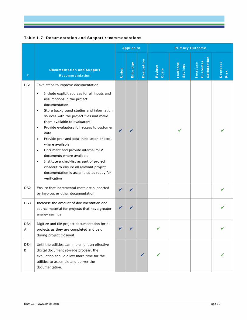
DNV GL – www.dnvgl.com Page 12
Table 1-7: Documentation and Support recommendations
#
Documentation and Support
Recommendation
Applies to Primary Outcome
Un
ion
Enb
rid
ge
Eval
uat
ion
Red
uce
Cos
ts
Incr
ease
Sav
ing
s
Incr
ease
Cu
sto
mer
Sat
isfa
ctio
n
Dec
reas
e
Ris
k
DS1 Take steps to improve documentation:
Include explicit sources for all inputs and
assumptions in the project
documentation.
Store background studies and information
sources with the project files and make
them available to evaluators.
Provide evaluators full access to customer
data.
Provide pre- and post-installation photos,
where available.
Document and provide internal M&V
documents where available.
Institute a checklist as part of project
closeout to ensure all relevant project
documentation is assembled as ready for
verification
DS2 Ensure that incremental costs are supported
by invoices or other documentation
DS3 Increase the amount of documentation and
source material for projects that have greater
energy savings.
DS4
A
Digitize and file project documentation for all
projects as they are completed and paid
during project closeout.
DS4
B
Until the utilities can implement an effective
digital document storage process, the
evaluation should allow more time for the
utilities to assemble and deliver the
documentation.

DNV GL – www.dnvgl.com Page 13
#
Documentation and Support
Recommendation
Applies to Primary Outcome
Un
ion
Enb
rid
ge
Eval
uat
ion
Red
uce
Cos
ts
Incr
ease
Sav
ing
s
Incr
ease
Cu
sto
mer
Sat
isfa
ctio
n
Dec
reas
e
Ris
k
DS5 Consider providing more training or adding
quality control steps to ensure the summary
workbook front page is completed and stored
in a consistent manner.
DS6 Use a consistent summary workbook.
Table 1-8: Data management recommendations
#
Data Management
Recommendation
Applies to Primary Outcome
Un
ion
Enb
rid
ge
Eval
uat
ion
Red
uce
Cos
ts
Incr
ease
Sav
ing
s
Incr
ease
Cu
sto
mer
Sat
isfa
ctio
n
Dec
reas
e
Ris
k
DM1
A
Track contacts associated with projects in the
program tracking database.
DM1
B
Strongly consider investing in relational
program tracking databases.
DM1
C
Include structure for improved data integrity
in the evaluator request for contact
information for the 2016 and 2017 savings
verification and evaluation.
DM2
A
Consider offering bonus incentives early in the
year to combat the “hockey stick”
phenomenon where a large percent of
projects get closed in the fourth quarter of the
year (which results in rushed QC for data).
DM3 Track and provide to evaluators dates for key
milestones in the project.
DM4 Maintain a customer identifier in the database
to clearly identify related sites.

DNV GL – www.dnvgl.com Page 14
#
Data Management
Recommendation
Applies to Primary Outcome
Un
ion
Enb
rid
ge
Eval
uat
ion
Red
uce
Cos
ts
Incr
ease
Sav
ing
s
Incr
ease
Cu
sto
mer
Sat
isfa
ctio
n
Dec
reas
e
Ris
k
DM5 Include EUL (also remaining useful life for
dual baselines), NTG, and each of the key
savings types (i.e., annual and cumulative,
gross and net) in the program tracking
extracts provided to evaluators.
Figure 1-1 shows an approximate cost vs. impact relation ship for each of the recommendations on a 4 point scale. The upper left quadrant of the figure shows the recommendations that are relatively low cost that would have a high impact. Those in the upper right are recommendations where both cost and impact are high.
Figure 1-1: Approximate Cost vs. Impact of each recommendation
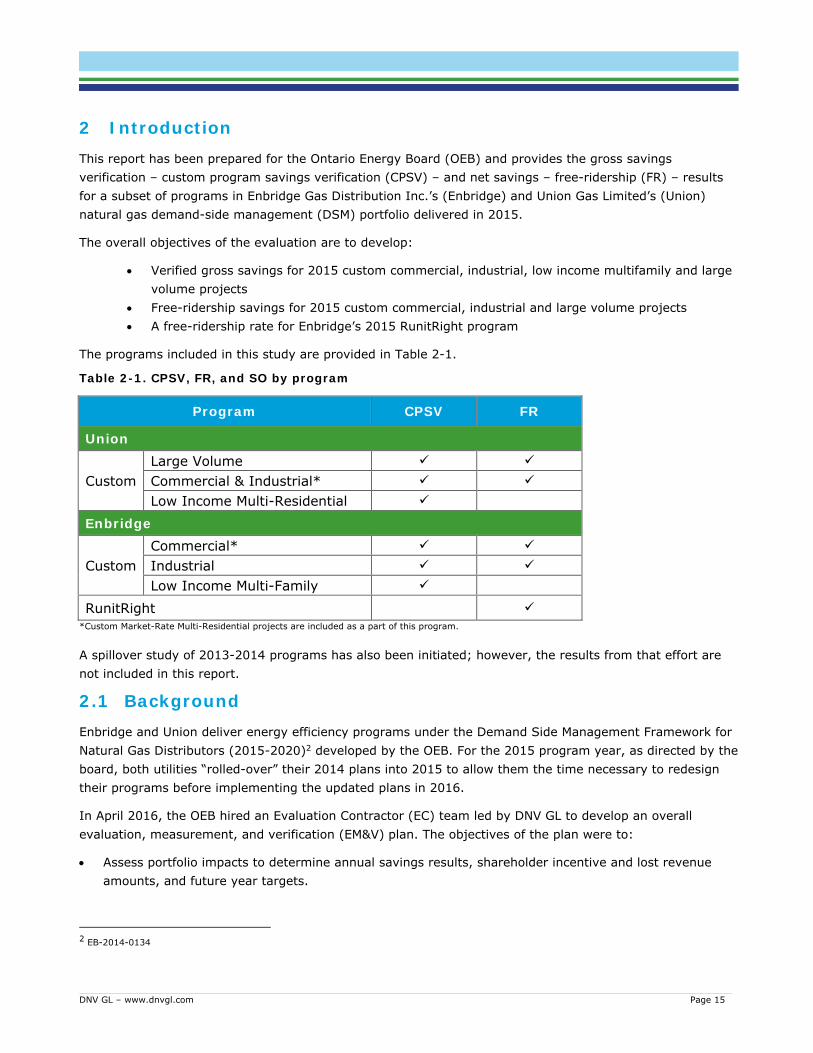
DNV GL – www.dnvgl.com Page 15
2 Introduction This report has been prepared for the Ontario Energy Board (OEB) and provides the gross savings verification – custom program savings verification (CPSV) – and net savings – free-ridership (FR) – results for a subset of programs in Enbridge Gas Distribution Inc.’s (Enbridge) and Union Gas Limited’s (Union) natural gas demand-side management (DSM) portfolio delivered in 2015.
The overall objectives of the evaluation are to develop:
Verified gross savings for 2015 custom commercial, industrial, low income multifamily and large volume projects
Free-ridership savings for 2015 custom commercial, industrial and large volume projects A free-ridership rate for Enbridge’s 2015 RunitRight program
The programs included in this study are provided in Table 2-1.
Table 2-1. CPSV, FR, and SO by program
Program CPSV FR
Union
Custom Large Volume
Commercial & Industrial*
Low Income Multi-Residential Enbridge
Custom Commercial*
Industrial
Low Income Multi-Family
RunitRight
*Custom Market-Rate Multi-Residential projects are included as a part of this program.
A spillover study of 2013-2014 programs has also been initiated; however, the results from that effort are not included in this report.
2.1 Background Enbridge and Union deliver energy efficiency programs under the Demand Side Management Framework for Natural Gas Distributors (2015-2020)2 developed by the OEB. For the 2015 program year, as directed by the board, both utilities “rolled-over” their 2014 plans into 2015 to allow them the time necessary to redesign their programs before implementing the updated plans in 2016.
In April 2016, the OEB hired an Evaluation Contractor (EC) team led by DNV GL to develop an overall evaluation, measurement, and verification (EM&V) plan. The objectives of the plan were to:
Assess portfolio impacts to determine annual savings results, shareholder incentive and lost revenue amounts, and future year targets.
2 EB-2014-0134

DNV GL – www.dnvgl.com Page 16
Assess the effectiveness of energy efficiency programs on their participants and/or market, including results on various scorecard items.
Identify ways in which programs can be changed or refined to improve their performance.
Under the plan, the DNV GL team conducted a CPSV and net-to-gross (NTG) study of the 2015 program year. This report is a result of that study.
An evaluation advisory committee (EAC) was formed to provide input and advice to the OEB on the evaluation and audit of DSM results. The EAC consists of representatives from utility representatives, non-utility stakeholders, independent experts, staff from the Independent Electricity System Operator (IESO), and observers from the Environmental Commissioner of Ontario and the Ministry of Energy. The DNV GL team worked closely with the EAC throughout this study and received comment, advice, and input on methodology and results. We than them for their involvement.
2.2 Methodology summary The results presented in this report are based on data collection from the following five primary sources, supplemented with secondary source information:
Union and Enbridge tracking databases Union and Enbridge project documentation In-Depth Interviews with a sample of participating customers In-Depth Interviews with a sample of participating vendors On-site visit to a sample of participating customer sites
The data collection with samples of participating customers and vendors included site visits and telephone interviews supporting a detailed measurement and verification (M&V) analysis, and in-depth interviews supporting assessment of free ridership. Table 2-2 shows the targeted and completed data collection activities and the timeframe in which they were completed.

DNV GL – www.dnvgl.com Page 17
Table 2-2. Data collection activities*
Target Group Activity Targeted Completed Timeframe
Enbridge
Participating Customers
M&V Site Visit (On-site) 41 61 Jan, 2017 - Mar, 2017
TSER Interview 38 37 Jan, 2017 - Apr, 2017
In-Depth Interview 149 151 Jan, 2017 - Apr, 2017
Participating Vendors In-Depth Interview ~30 20 Mar, 2017- Apr, 2017
Union
Participating Customers
M&V Site Visit (On-site) 59 106 Jan, 2017 - Mar, 2017
TSER Interview 22 30 Jan, 2017 - Apr, 2017
In-Depth Interview 122 203 Jan, 2017 - Apr, 2017
Participating Vendors In-Depth Interview ~30 15 Mar, 2017- Apr, 2017
Overall
Participating Customers
M&V Site Visit (On-site) 100 167 Jan, 2017 - Mar, 2017
TSER Interview 60 67 Jan, 2017 - Apr, 2017
In-Depth Interview 271 354 Jan, 2017 - Apr, 2017
Participating Vendors In-Depth Interview ≤62 35 Mar, 2017- Apr, 2017
*This table reports the number of units of analysis targeted and completed as units of analysis were used to design the sample before customers and sites had been identified. Units of Analysis are a slight aggregation of utility tracking records as described in APPENDIX I.
At a high level, the CPSV and NTG study employed the following methodology:
Receive program data and documentation. The evaluation started with a review of the program tracking data, which formed the basis of the sample, and an initial review of the program documentation. Once the sample was selected, additional documentation was provided by the program to describe the energy efficiency measures and support the tracking savings estimates, also called the ex ante estimates.
Design and select the sample. The tracking data was used to design and select a sample. Full documentation and contact information was requested for all sites within the sample. The CPSV sample was designed as a subset of the NTG sample.
Collect data. Data was collected to verify the ex ante energy savings and estimate NTG ratios. Analyze the results. The collected data was used to verify the gross savings and estimate NTG ratios
at each site. Report the results. The final step was to report the results.

DNV GL – www.dnvgl.com Page 18
Key features of the methodology include:
The sample design employed a stratified random sample that targeted 10% relative precision with 90% confidence at the program level. Details of the sampling methods are presented in APPENDIX I. Final sample achievements are provided in APPENDIX A.
Ratio estimation was used to expand sample results to the population. The evaluation collected data on all projects that a customer contact could speak to rather than only the first selected. This means that the evaluation exceeded the targeted number of sampled units in the measure level sample design. In the expansion, weights were adjusted to eliminate potential bias from this data collection strategy by assigning a weight of one (1) to non-randomly selected units. In our calculation of sampling error (+/-, confidence intervals, relative precision and error ratios), we used two tailed 90-percent confidence limits and clusters defined by customers to appropriately estimate error when multiple units are collected from a single source.3 The approach used is described in APPENDIX M.
The gross savings verification used a combination of on-site data collection and interviews to collect primary data. Calculation of lifetime gross savings used a dual baseline approach to more accurately estimate savings for early replacement measures. More information on the verification approach is provided in APPENDIX B, APPENDIX O, and APPENDIX P. Detailed site reports for each of the sites visited or called are provided in a volume 2 and 3 of this report.
The NTG methodology included data collection from participating customers and vendors. The data collection instrument outlines are provided in APPENDIX N. NTG scoring methods are provided in APPENDIX J and APPENDIX K.
2.2.1 Understanding Statistical Error Statistical error is reported for all of the ratio results in this report. The studies were designed with sample designs targeting 10% relative precision with 90% confidence (90/10) based on the best available assumptions at the start of the evaluation. Table 2-3 describes each of the statistics provided in this report.
The relative precision of some of the ratios is low because the ratios themselves are small. Relative precision is the absolute precision (+/- quantity) divided by the estimated ratio. For example, if a ratio is 5% with absolute precision of +/-5%, the relative precision is very bad (5%/5% = 100% relative error) but in absolute terms we still are 90% confident the ratio is below 10%, which is useful information. We reported the relative precision in all cases at the 90 percent confidence level. That is, whether the relative precision is large or small, we have the same 90 percent confidence that the range defined by the point estimate +/- the absolute error captures the true unknown value. The “midpoint” estimate is the best (statistically most likely) estimate, while the confidence interval is calculated as an interval around that point. Thus, in all cases, we reported the best point estimate, with a symmetric 90% confidence interval (using the t-score for a 2-tailed 90% confidence interval).
3 Where a single site had two contacts, the site was used as the cluster to ensure conservative (higher) error estimates.

DNV GL – www.dnvgl.com Page 19
Table 2-3: Relevant statistics.
Term Definition
Ratio/Adjustment factor
A point estimate of the evaluation findings expressed as a percent.
+/- or Absolute Precision
If the evaluation were repeated several times selecting samples from the same population, 90%4 of the time the ratio would be within this range of the ratio
Confidence interval The upper bound is defined by the ratio plus the absolute precision. the lower bound is defined by the ratio minus the absolute precision.
Relative Precision The relative precision is calculated as the absolute precision divided by the ratio itself. By convention, relative precisions are the statistic that are targeted in sampling (i.e., 90/10 is a relative precision metric)
Error Ratio The error ratio is an approximation of the coefficient of variation (cv) that is used in sample design. It is calculated as a function of relative precision.
Finite population correction (FPC)
FPC is a factor that reduces the measured error of samples drawn from small populations (less than 300). FPC applies when the ratio is applied to the same population from which the sample was drawn. Statistics reported in the body of this report all employ the FPC factor.
Figure 2-1 shows an example:
the adjustment factor (ratio) as a blue point
the 90% confidence interval with finite population correction (blue)
the 90% confidence interval without finite population correction (green)
Figure 2-1: Ratio diagram example
4 90% is the confidence limit that we are using.
Adjustment Factor
90 Percent Confidence Interval, Without Finite Population Correction
90 Percent Confidence Interval, Finite Population Correction
89% 99%94%

DNV GL – www.dnvgl.com Page 20
The plus/minus (±) error (%) indicated at the 90% confidence interval is the absolute difference between the estimated percentage and the upper or lower confidence bound. For example, in Figure 2-1, the ratio is 94% and the non-FPC 90% confidence interval is ± 5 percentage points (i.e., 94% ± 5%).5 Another way of saying this is that there is a 90% probability that the actual ratio for the next year’s program lies between 89 and 99%. Figure 2-2 demonstrates this concept by showing twenty hypothetical confidence intervals calculated from twenty different samples of the same population. Eighteen out of twenty (90%) include the true population ratio (overlap the black line representing the true ratio).
Figure 2-2. Ninety Percent Confidence Interval
Note: Each horizontal line represents a confidence interval, while the black vertical line is the actual population realization rate. Yellow confidence
intervals do not include the actual ratio.
The relative precision of the ratio is calculated as 5%/94% =5.3%.
For low ratios, relative precisions may be quite high, even when the confidence interval around the ratio is quite narrow. Consider a ratio of 5% with the same 5% absolute precision as in the above example. While the absolute precisions are the same, the latter ratio (5%) has a relative precision of 5%/5% =100%. In absolute terms, we still are 90% confident the ratio is below 10%, despite the very high (100%) relative precision.
We reported the relative precision in all cases at the 90 percent confidence level. That is, whether the relative precision is large or small, we have the same 90 percent confidence that the range defined by the point estimate +/- the absolute error captures the true unknown value. The “midpoint” estimate (the ratio) is the best (statistically most likely) estimate, while the confidence interval is calculated as an interval around that point. Thus, in all cases, we reported the best point estimate, with a symmetric 90% confidence interval (using the t-score for a 2-tailed 90% confidence interval).
5 The critical value for calculating the confidence interval ± for each adjustment factor is determined using Student's t-distribution and n-1 for the
degrees of freedom, where n is the sample size. The critical value for the gross savings adjustment factor is determined using the degrees of freedom based on the minimum sample size for the components of the adjustment factor. The gross savings adjustment factor is a product of the installation rate and the engineering verification factor. For 2-tailed estimates (ratios that could be above or below 100%) the appropriate t-stat used to calculate precision from the standard error is close to 1.645.

DNV GL – www.dnvgl.com Page 21
3 Union Commercial, Industrial, and Multi-Family Programs Through its custom program offerings, Union seeks to influence customers to adopt more energy efficient technologies and practices, or do so sooner than they would otherwise have done. The custom programs provide financial incentives, technical expertise, and guidance with respect to energy related decision-making. Union’s custom programs differ from the prescriptive and direct install programs as they provide services and varying financial incentives based on overall natural gas savings realized by the customer to address customer-specific needs.
There are three program offerings covered in this section: Union Commercial and Industrial Custom and Low Income Multi-Residential Affordable Housing.
3.1 Commercial and Industrial Custom Program Union advances customer energy efficiency and productivity by providing a mix of custom incentives, education and awareness to C&I customers across all segments. The objective of the Custom offering is to generate long‐term and cost effective energy savings for Union’s customers.
The Union Custom program covers opportunities where energy savings are linked to unique building specifications, design concepts, processes and new technologies that are outside the scope of prescriptive and quasi‐prescriptive measures. The program and incentives are targeted directly to the end user.
A subset of the projects in these programs is part of the multi-family or multi-residential segment (MR MF).
All projects implemented as part of these programs and claimed in 2015 are included in the CPSV and FR portions of the study.
3.2 Low-income Multi-Family Program (Union) The Union Low Income Multi-Family (LIMF) program offers multi-family low income housing customers funding for energy audits and both custom and prescriptive incentives to encourage energy efficient upgrades and funding for energy audits. The programs also provide technical services, benchmarking, and education for housing providers, building operators and tenants about their building’s energy usage and ways to achieve energy efficiency.
The target markets for both programs are social and assisted housing providers who own and operate Part 3 buildings and private multi-residential building owners that provide housing to low income households.6
Custom projects implemented as part of these programs and claimed in 2015 are included in the CPSV portion of the study; 12% of Union’s LIMF program savings are from custom projects. An evaluation of this program’s net-to-gross (NTG) was not included in this study.
3.3 CPSV results This section summarizes the gross savings verification (CPSV) results for custom projects in the Union commercial, industrial, multifamily, and low income multi-family programs. For Union, the gross realization rate is made up of two components, the influence correction which removes Union’s influence adjustments
6 “Part 3” references buildings covered by Part 3 of the Ontario Building Code, defined as those exceeding 600 square meters in area or greater than
three storeys in height; for residential energy efficiency programs, these are typically multifamily buildings.

DNV GL – www.dnvgl.com Page 22
from the tracking gross savings, and the engineering adjustment, which provides the difference (expressed as a ratio) between verified savings determined through the CPSV and tracked gross savings estimated by Union prior to applying the influence adjustment. The gross realization rate is the product of the influence correction and the engineering adjustment.
Section 3.3.1 summarizes the data collection efforts, section 3.3.2 describes and presents the influence correction, section 3.3.3 describes and presents the engineering adjustment, section 3.3.4 summarizes the reasons for the discrepancies between the ex ante and ex post gross savings estimates, and section 3.3.5 presents the gross savings realization rate.
3.3.1 Summary of CPSV data collection Table 3-1 summarizes the CPSV data collection efforts for the Union Custom C&I, and LIMF programs. The table shows the portion of the program that:
Completed on-site visits Completed telephone supported engineering reviews (TSER) Did not respond to an evaluation attempt at contact Was not contacted by the evaluation team.7
The data collected is represented as the number of sites, the number of projects, the number of units of analysis, and cumulative ex ante natural gas savings (ex ante CCM). The proportion of the program in each category is also represented in Figure 3-1. The full sample design and achievement by strata can be found in 8. By collecting data on all measures at a site rather than only the first selected, the evaluation exceeded the targeted number of units despite collecting data from fewer sites. The study had a customer response rate of 64% and achieved the targeted 90/10 relative precision for the gross realization rate at the program overall level shown in Table 3-4).
Table 3-1: Summary of CPSV data collection for Union Custom C&I, and LIMF programs*
Data Collection Category
Targeted Completed
# Units of Analysis # Sites #
Measures
# Units of
Analysis Ex Ante CCM
Completed On-Site 38 35 77 62 595,857,289 Completed TSER 22 22 37 30 93,508,182 Attempted Contact, Not Completed 32 66 47 226,355,899
Not Attempted 337 445 389 564,118,008 Total 426 625 528 1,479,839,378
* Please see the glossary for definitions of unit of analysis, site, and project.
7 Sites, projects, or units of analysis where contact was not attempted were either not selected for contact in sampling or in the backup sample and
were not contacted due to strata quotas being met.

DNV GL – www.dnvgl.com Page 23
Figure 3-1: Summary of CPSV data collection for Union Custom C&I, MF, and LIMF programs
3.3.2 Influence correction The Union Custom C&I, MF, and LIMF programs had some corrections and adjustments that differ from other programs: the influence correction and the engineering adjustment.
The Union implementation team applied a proactive “influence factor” to some measures. The factor represents the portion of the energy savings that, in the opinion of the implementation team, was influenced by the program. In effect, it represents an anticipated free-ridership adjustment. Since the evaluation team is measuring and applying a retrospective free-ridership adjustment based on customer self-reports, the Union influence factor would double-count free-ridership for those measures. Therefore, the evaluation team removed the influence factor to produce a “true” gross savings estimate to which the NTG adjustment could be applied. Because the influence factor was not tracked for the population, we worked with Union to identify the influence factors made to the sample of projects selected for CPSV and reversed the process to calculate a true gross tracking savings. This process resulted in the influence corrections provided below.
Table 3-2 shows the influence correction by domain for the Union Custom C&I, MF, and LIMF programs. The table shows the number of units of analysis (n), influence correction ratio, precision at the 90% confidence interval, error ratio, and percent of program savings. The percent of program savings represents the relative contribution that each domain makes to the overall result. Note that Custom Industrial Actions and Custom Commercial & Multi-family received ratios, or influence corrections, of 103% and 101%, respectively. A ratio of 103% indicates that for these measures Union recorded 97% of the gross savings in its database. The positive (greater than 100%) adjustment was made to reported tracked savings to remove the influence factors assigned.

DNV GL – www.dnvgl.com Page 24
Table 3-2: Influence correction for Union Custom C&I and LIMF programs
Sector Domain n
Ratio 90% Confidence Interval
Error Ratio
% Program Savings Measures Clusters +/- Lower
Bound Upper Bound
Relative Precision
Custom Industrial
Greenhouse Equipment 15 9 100% 0% 100% 100% 0% 0.00 29%
Action 20 12 103% 4% 99% 106% 3% 0.07 12%
Hydronic Insulation 9 9 100% 0% 100% 100% 0% 0.00 8%
Other Equipment 36 25 100% 0% 100% 100% 0% 0.00 33%
Custom Commercial and LIMF 34 24 101% 2% 100% 103% 2% 0.05 19%
Overall 114 74 101% 1% 100% 101% 1% 0.03 100%
The Other category includes building shell equipment, controls, heat recovery, HVAC, operational improvements, steam separator, reverse osmosis, refractory insulation, high-efficiency iron converters, robotic arms, infrared coating, and damper motor replacement
APPENDIX M describes the criteria used for determining the domains used for ratio application and reporting. Clusters reported in this table are unique customers per stratum: one customer may be in multiple strata, so the count of clusters is greater than the
number of customers contacted. Confidence intervals are mathematically correct, but in practical terms, the influence correction can only be equal to or greater than 100%.
3.3.3 Engineering adjustment For programs with an influence adjustment, such as the Union Custom C&I, MF, and LIMF programs, the evaluation team defined an “engineering adjustment.” This ratio is the difference between verified savings determined through the CPSV and tracked gross savings estimated by Union prior to applying the influence adjustment. These changes are due to differences in calculation methods, effective useful life (EUL), calculation parameters, or other engineering-related adjustments. The engineering adjustment is equivalent to the gross savings realization rate for programs that do not have an influence adjustment.
Table 3-3 shows the engineering adjustment by domain for the Union Custom C&I, MF, and LIMF programs. The table shows the number of units of analysis (n), engineering adjustment ratio (Ratio), precision at the 90% confidence interval, error ratio, and percent of program savings. The percent of program savings represents the relative contribution that each domain makes to the overall result. Overall, the engineering adjustment was 99%. The measure group with the highest adjustment was Hydronic Insulation, due to different operating conditions (temperatures and hours) reported than were documented in the ex ante calculations at four of nine sites. The measure group with the lowest adjustment was greenhouse equipment, primarily due to measure realization rates of ~80% for 4 of the 15 measures. The discrepancies found at these sites include changes to baseline and efficient conditions.

DNV GL – www.dnvgl.com Page 25
Table 3-3: Engineering adjustment for Union Custom C&I and LIMF programs
Sector Domain n
Ratio 90% Confidence Interval Error
Ratio %
Program Savings
Measures Clusters +/- Lower Bound
Upper Bound
Relative Precision
Custom Industrial
Greenhouse Equipment 15 9 92% 4% 88% 95% 4% 0.06 29%
Action 20 12 105% 13% 92% 118% 13% 0.24 12% Hydronic Insulation 9 9 116% 11% 105% 127% 9% 0.15 8% Other Equipment 36 25 101% 15% 86% 116% 15% 0.43 33%
Custom Commercial and Multi-family 34 24 88% 18% 70% 106% 21% 0.59 19%
Overall 114 74 98% 6% 92% 105% 6% 0.33 100% The Other Equipment category includes building shell equipment controls, heat recovery, HVAC, operational improvements, steam separator, reverse
osmosis, refractory insulation, high-efficiency iron converters, robotic arms, infrared coating, and damper motor replacement. APPENDIX M describes the criteria used for determining the domains used for ratio application and reporting. Clusters reported in this table are unique customers per stratum: one customer may be in multiple strata, so the count of clusters is greater than the
number of customers contacted.
Figure 3-2 also shows the engineering adjustment by domain. The figure shows the ratio point estimate as a blue dot on the horizontal axis and the confidence interval as hashmarks connected by a green line. The number of units of analysis, numeric ratio, and percent of program savings represented by each domain are shown to the right of the plot. Industrial greenhouse equipment and hydronic insulation are the only domains that are statistically significantly different from 100%.

DNV GL – www.dnvgl.com Page 26
Figure 3-2: Engineering adjustment for Union Custom C&I, and LIMF programs
3.3.4 Discrepancy summary This section presents detailed results for the reasons for and magnitude of the various discrepancies between ex ante and ex-post savings. First we will look at the cumulative savings, then the two key components of cumulative savings: annual savings and the EUL. See APPENDIX Q for additional detail.
Figure 3-3 plots the ex post cumulative savings (with influence corrected) against the ex ante cumulative savings (with influence corrected) for each measure in the sample. The plot on the left shows the full set of measures, while the plot on the right is focused in on the cluster of measures with less than 10 million CCM in both ex ante and ex post. The diagonal line represents a 100% engineering adjustment, or the plotted value if ex post equals ex ante. Points above the line indicate measures where ex post savings were greater than ex ante, while points below the line indicate where ex post were less than ex ante.
Most projects had similar ex post and ex ante savings. The largest two sites had large discrepancies. The largest was a thermal oxidator project that had a realization rate of 127% (upper right) due to operating conditions differences in the ex ante and ex post cases. The second was a new construction project with a 55% realization rate: in this case the code used for the ex ante baseline was outdated at the time that building permits were applied for.

DNV GL – www.dnvgl.com Page 27
Figure 3-3. Ex post versus ex ante cumulative savings (CCM) with influence corrected - Union C&I and MF, by measure type
3.3.4.1 First-year savings discrepancies Figure 3-4 plots the ex post annual savings (with influence corrected) against the ex ante annual savings (with influence corrected) for each measure in the sample. The plot on the left shows the full set of measures, while the plot on the right is focused in on the cluster of measures with less than 0.20 million cubic meters (m3) in both ex ante and ex post. The diagonal line represents a 100% engineering adjustment, or the plotted value if ex post equals ex ante. Points above the line indicate measures where ex post savings were greater than ex ante, while points below the line indicate where ex post were less than ex ante.
The plot on the left shows a very similar pattern to that of the cumulative savings because the two largest projects and adjustments were each due to discrepancies in annual savings. The plot on the right shows some differences because annual savings were adjusted for several controls projects. There was no pattern to the discrepancies in this case: one was a difference in baseline between ex ante and ex post, one involved additional data provided to the verifier and one lowered production after the program measure was implemented.
Zoom in on <=10 million CCM

DNV GL – www.dnvgl.com Page 28
Figure 3-4: Ex post versus ex ante annual savings with influence corrected - Union C&I, by measure type
3.3.4.2 Measure life discrepancies One of the primary discrepancies is a change in EUL between ex ante and ex post. Figure 3-5 plots the ex post EUL against the ex ante EUL for each measure in the sample. Because EULs tend to be discrete numbers, the size of the bubbles in the plot indicate show the relative amount of ex ante savings for the measures at each plotted point (e.g., the larger the bubble, the more savings at that point). The diagonal line represents the plotted value if ex post equals ex ante. Points above the line indicate measures where ex post EUL were greater than ex ante, while points below the line indicate where ex post were less than ex ante.
The plot shows that most EULs had equal ex post and ex ante EULs. The projects with the greatest differences tended to be small to medium sized and differences in EUL went both ways. Some projects had greater EULs in the ex post than the ex ante and vice versa. The overall weighted average EUL adjustment for the program was 99.8%.
Zoom in on <= 0.20 million CCM

DNV GL – www.dnvgl.com Page 29
Figure 3-5: Ex post versus ex ante effective useful life - Union C&I and MF, by measure type
3.3.5 Gross realization rate For the Union programs, the gross realization rate is the product of the influence correction and the engineering adjustment. Table 3-4 shows the engineering adjustment by domain for the Union Custom C&I, MF, and LIMF programs. The table shows the number of units of analysis (n), engineering adjustment ratio (Ratio), precision at the 90% confidence interval, error ratio, and percent of program savings. The percent of program savings represents the relative contribution that each domain makes to the overall result.
Union’s C&I and LIMF programs overall had a 100% gross realization rate, which means that the overall ex post savings are equivalent to the overall ex ante savings, within rounding errors. The Action domain has a gross realization rate pf 108%, the result of an influence correction of 103% and an engineering adjustment of 105%. Likewise, Custom Commercial, and LIMF result in a ratio of 97%, the result of a 101% influence correction and 95% engineering adjustment.

DNV GL – www.dnvgl.com Page 30
Table 3-4: Gross realization rate for Union Custom C&I and LIMF programs
Sector Domain n
Ratio 90% Confidence Interval Error
Ratio %
Program Savings
Measures Clusters +/- Lower Bound
Upper Bound
Relative Precision
Custom Industrial
Greenhouse Equipment 15 9 92% 4% 88% 95% 4% 0.06 29%
Action 20 12 108% 14% 94% 122% 13% 0.25 12% Hydronic Insulation 9 9 116% 11% 105% 127% 9% 0.15 8%
Other Equipment 36 25 101% 15% 86% 116% 15% 0.43 33%
Custom Commercial and LIMF 34 24 89% 18% 71% 108% 21% 0.59 19%
Overall 114 74 99% 6% 92% 105% 7% 0.34 100% The Other Equipment category includes building shell equipment controls, heat recovery, HVAC, operational improvements, steam separator, reverse
osmosis, refractory insulation, high-efficiency iron converters, robotic arms, infrared coating, and damper motor replacement. APPENDIX M describes the criteria used for determining the domains used for ratio application and reporting. Clusters reported in this table are unique customers per stratum: one customer may be in multiple strata, so the count of clusters is greater than the
number of customers contacted. *Overall ratio in this table is the sample weighted average and is not used in calculating gross savings for the programs.
Table 3-5 shows the influence correction and engineering adjustments that were multiplied to calculate the gross realization rates.
Table 3-5: Gross realization rate components for Union Custom C&I and LIMF programs
Sector Domain Influence correction
Engineering Adjustment
Gross Realization
Rate
Custom Industrial
Greenhouse Equipment 100% 92% 92%
Action 103% 105% 108% Hydronic Insulation 100% 116% 116%
Other Equipment 100% 101% 101%
Custom Commercial and LIMF 101% 88% 89%
Overall 101% 98% 99%
3.4 NTG ratio This section summarizes the free-ridership results for the Union Custom C&I, MF, and LIMF programs. Section 3.4.1 summarizes the data collection efforts, section 3.4.2 presents the net savings realization rate, and section 3.4.3 describes the sources of program attribution.
3.4.1 Summary of participant data collected Table 3-6 summarizes the NTG ratio data collection efforts for the Union Custom C&I, MF, and LIMF programs. The table shows the portion of the program that:
Completed an in-depth interview through the NTG battery Did not respond to an evaluation attempt at contact
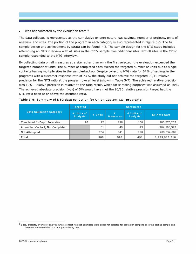
DNV GL – www.dnvgl.com Page 31
Was not contacted by the evaluation team.8
The data collected is represented as the cumulative ex ante natural gas savings, number of projects, units of analysis, and sites. The portion of the program in each category is also represented in Figure 3-6. The full sample design and achievement by strata can be found in 8. The sample design for the NTG study included attempting an NTG interview with all sites in the CPSV sample plus additional sites. Not all sites in the CPSV sample responded to the NTG interview.
By collecting data on all measures at a site rather than only the first selected, the evaluation exceeded the targeted number of units. The number of completed sites exceed the targeted number of units due to single contacts having multiple sites in the sample/backup. Despite collecting NTG data for 67% of savings in the programs with a customer response rate of 73%, the study did not achieve the targeted 90/10 relative precision for the NTG ratio at the program overall level (shown in Table 3-7). The achieved relative precision was 12%. Relative precision is relative to the ratio result, which for sampling purposes was assumed as 50%. The achieved absolute precision (+/-) of 5% would have met the 90/10 relative precision target had the NTG ratio been at or above the assumed ratio.
Table 3-6: Summary of NTG data collection for Union Custom C&I programs
Data Collection Category
Targeted Completed
# Units of Analysis # Sites #
Measures # Units of Analysis Ex Ante CCM
Completed In-Depth Interview 90 92 198 150 980,275,237
Attempted Contact, Not Completed 31 49 43 204,588,592
Not Attempted 266 341 298 289,054,889
Total 389 588 491 1,473,918,718
8 Sites, projects, or units of analysis where contact was not attempted were either not selected for contact in sampling or in the backup sample and
were not contacted due to strata quotas being met.

DNV GL – www.dnvgl.com Page 32
Figure 3-6: Summary of NTG data collection for Union Custom C&I, MF, and LIMF programs
3.4.2 Free-ridership Free-ridership is the sole contributor to the NTG ratio. The evaluation team is also conducting a study of the spillover savings attributable to the program; spillover results will be presented in a later report. Free-ridership is calculated from self-reported responses to survey questions as outlined in APPENDIX C.
Table 3-7 shows the NTG ratio by domain for the Union Custom C&I programs. The table also shows the number of units of analysis (n), precision at the 90% confidence interval, error ratio, and percent of program savings. The percent of program savings represents the relative contribution that each domain makes to the overall result.

DNV GL – www.dnvgl.com Page 33
Table 3-7: NTG ratio for Union Custom C&I programs
Sector Domain n
NTG Ratio
90% Confidence Interval Error Ratio
% Program Savings Meas Clusts +/- Lower
Bound Upper Bound
Relative Precision
Custom Industrial
Greenhouse 26 17 40% 12% 28% 52% 30% 0.70 29%
Heat Recovery 29 21 59% 7% 52% 66% 12% 0.32 20% Leak Repair and Hydronic Insulation
26 21 40% 9% 30% 49% 24% 0.63 14%
Operational Improvements 9 7 10% 9% 1% 19% 85% 1.16 4%
Controls 7 7 18% 4% 14% 22% 21% 0.29 2%
Steam Trap 6 6 29% 12% 17% 41% 42% 0.52 2%
Other 33 23 21% 10% 11% 31% 49% 1.37 10%
Custom Commercial
Controls 16 6 78% 5% 74% 83% 6% 0.07 3%
Other 46 23 38% 12% 26% 50% 32% 0.90 16%
Overall 198 112 39% 5% 34% 44% 12% 0.76 100% The Industrial Other category includes: building shell, HVAC, steam separator, reverse osmosis, refractory insulation, boiler, high-efficiency iron
converters, robotic arms, duct insulation, infrared coating, and damper motor replacement. The Commercial Other category includes: building shell, heat recovery, HVAC, hydronic insulation, leak repair, operational improvements, steam traps,
high-efficiency washer, domestic hot water upgrade, air handling unit maintenance, and geothermal heating. APPENDIX M describes the criteria used for determining the domains used for ratio application and reporting. Clusters reported in this table are unique customers per stratum: one customer may be in multiple strata, so the count of clusters is greater than the
number of customers contacted. *Overall ratio in this table is the sample weighted average and is not used in calculating net savings for the programs.
Figure 3-7 also shows the NTG ratio by domain. The figure shows the ratio point estimate as a blue dot on the horizontal axis and the confidence interval as hashmarks connected by a green line. The number of units of analysis, the numeric ratio, and the percent of program savings represented by each domain are shown to the right of the plot. The confidence intervals for all but the two lowest and two highest performing measures overlap the program overall ratio of 39%.
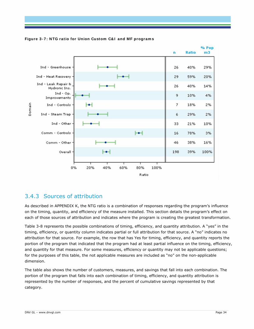
DNV GL – www.dnvgl.com Page 34
Figure 3-7: NTG ratio for Union Custom C&I and MF programs
3.4.3 Sources of attribution As described in APPENDIX K, the NTG ratio is a combination of responses regarding the program’s influence on the timing, quantity, and efficiency of the measure installed. This section details the program’s effect on each of those sources of attribution and indicates where the program is creating the greatest transformation.
Table 3-8 represents the possible combinations of timing, efficiency, and quantity attribution. A “yes” in the timing, efficiency, or quantity column indicates partial or full attribution for that source. A “no” indicates no attribution for that source. For example, the row that has Yes for timing, efficiency, and quantity reports the portion of the program that indicated that the program had at least partial influence on the timing, efficiency, and quantity for that measure. For some measures, efficiency or quantity may not be applicable questions; for the purposes of this table, the not applicable measures are included as “no” on the non-applicable dimension.
The table also shows the number of customers, measures, and savings that fall into each combination. The portion of the program that falls into each combination of timing, efficiency, and quantity attribution is represented by the number of responses, and the percent of cumulative savings represented by that category.

DNV GL – www.dnvgl.com Page 35
The table shows that the majority program participation (58% of savings) at least partially influenced by the program. Of the three ways the program can influence program performance, timing is the most common, affecting approximately 49% of the program savings.
Table 3-8. Overview of the sources of attribution for Union Custom C&I programs
Attribution
Timing Efficiency Quantity Customers* Units of Analysis Projects Percent
Savings Yes Yes Yes 11 20 31 14% Yes Yes No * * * 9% Yes No Yes 16 34 44 14% Yes No No 19 25 34 13% No Yes Yes * * * <1% No Yes No 5 6 6 6% No No Yes 7 7 13 3% No No No 41 55 66 41%
For confidentiality reasons the numbers of customers, units of analysis and measures less than 5 are not displayed. A customer may appear multiple times if their responses varied by measures, resulting in a total greater than the number of customers interviewed.
3.4.3.1 Timing Respondents answered a sequence of questions that addresses the timing of the equipment installation. First, respondents answered the likelihood of installing the same type of equipment at the same time without the program (DAT1a). Respondents who answered “Later” specified the number of months later in the next question (DAT1b).9
Timing was the component most strongly affected by the program. The program affected the timing of projects that account for approximately half of the energy savings. Fifty-two customers accounting for 51% of program savings said they would have installed their measure(s) at the same time. Projects accounting for approximately 17% of savings received full attribution by answering that they never would have installed the measure (13% of savings) or would have delayed the project by 48 months or more (4% of savings). The remaining 33% of savings received partial timing attribution (Table 3-9).
9 See APPENDIX K for the detailed scoring algorithm.

DNV GL – www.dnvgl.com Page 36
Table 3-9. Determining the acceleration period, Union Custom C&I programs
DAT1a. Without the utility, how different would the timing have been? DAT1b. Approximately how many months later?
DAT1a DAT1b Customers* Units of Analysis Projects Percent
Savings Timing
Attribution Same Time N/A 52 69 87 50% 0% Earlier N/A 0 0 0 0% 0%
Later
Months < 48 24 43 57 25%
ER baseline credit** for
months accelerated
Months >= 48 * 6 10 4% 100%+ ER baseline credit
Don't Know/ Refused 8 12 16 7% ER baseline credit
for avg. of DAT1b Never N/A 12 20 28 13% 100% Don't Know/ Refused N/A 0 0 0 0% ER baseline credit
for avg. of DAT1a For confidentiality reasons the numbers of customers, units of analysis and measures less than 5 are not displayed. *A customer may appear multiple times if their responses varied by measures, resulting in a total greater than the number of customers interviewed. **ER baseline credit reflects credit for a vs. in situ equipment baseline savings during the acceleration period.

DNV GL – www.dnvgl.com Page 37
3.4.3.2 Efficiency Respondents answered a sequence of questions that addresses the program’s effects on the efficiency level of the installed equipment. First, respondents answered the likelihood of installing the same level of efficiency without the program (DAT2a). Respondents who answered that they would have installed a less efficient option answered a follow-up question (DAT2b) to specify the level of efficiency they would have installed.
The program had less effect on efficiency than timing, affecting approximately one-third (29%) of the program savings (Table 3-10). Approximately one-third (36%) of program savings received zero attribution because the respondents indicated they would have installed the same level of efficiency without the program. Another third (35%) of savings were from measures for which efficiency levels is not applicable such as operational improvements, leak repairs or steam trap replacements.
Table 3-10. Determining efficiency attribution, Union Custom C&I programs
DAT2a. Without the utility, would you have installed the same, higher, or lower efficiency? DAT2b. Without the utility, what efficiency would you have installed?
DAT2a DAT2b Customers* Units of Analysis Projects Percent
Savings Efficiency
Attribution
Same N/A/ Skipped 35 44 63 36% 0%
Lower
Standard Efficiency 9 17 25 10% 100%
Between Standard and High * * 6 11% 50%
Don't Know/ Refused * 7 9 8% Average of
DAT2b Higher N/A/ Skipped 0 0 0 0% 0%
Don't Know/Refused N/A Skipped * * * <1% Average of DAT2a
Not Applicable N/A 47 77 94 35% Not Asked For confidentiality reasons the numbers of customers, units of analysis and measures less than 5 are not displayed. A customer may appear multiple times if their responses varied by measures, resulting in a total greater than the number of customers interviewed.

DNV GL – www.dnvgl.com Page 38
3.4.3.3 Quantity Respondents answered a sequence of questions that addresses the program’s effects on the amount of equipment installed. First, respondents answered the likelihood of installing the same amount of equipment (or capacity for measures for which number is not relevant, such as chillers) without the program (DAT3a). Respondents who answered that they would have installed a less or more equipment answered a follow-up question (DAT3b) to specify how the program changed the amount that they installed.
The program had about the same level of effect on quantity as efficiency, affecting approximately one-third (29%) of the program savings (Table 3-11). Approximately two-thirds (66%) of program savings received zero attribution because the respondents indicated they would have installed the same amount without the program.
Table 3-11. Determining quantity/size attribution, Union Custom C&I programs
DAT3a. Without the utility, how different would the quantity/size have been? DAT3b. By what percentage did you change the amount installed because of utility?
DAT3a DAT3b Customers* Units of Analysis Projects Percent
Savings Quantity
Attribution
Same N/A 58 84 107 66% 0%
Less
Value < 100% 10 14 29 10% Value < 50% Value ≥ 100% * * * <1% Value > 50% Don't Know/Refused 6 19 22 4% Average of DAT3a
More
Value < 100% 0 0 0 0% Value < 100% Value ≥ 100% 0 0 0 0% Value = 100% Don't Know/ Refused 0 0 0 0% Average of DAT3a
None N/A 11 22 29 16% 100% Don't Know/ Refused N/A * * * <1% Average of DAT3
Not Applicable N/A 7 9 9 4% Not Asked For confidentiality reasons the numbers of customers, units of analysis and measures less than 5 are not displayed. A customer may appear multiple times if their responses varied by measures, resulting in a total greater than the number of customers interviewed.
3.5 Gross and net savings This section reports the evaluation-verified gross savings in section 3.5.1 and the net savings (including only free-ridership) in section 3.5.2.
3.5.1 Verified gross savings The program-level gross savings are determined by multiplying tracked savings by the gross realization rate within each primary reporting domain. Table shows the primary domains, tracked savings, gross realization rate (RR), and final verified gross savings. Dividing the overall verified gross savings by the overall tracking savings results in a program-level gross realization rate of 99%.

DNV GL – www.dnvgl.com Page 39
Table 3-12: Verified gross savings for Union Custom C&I and LIMF programs
Sector Applied Domain Cumulative
Tracked Savings (m3)
Gross RR
Verified Cumulative
Gross Savings (m3)
Custom Industrial
Greenhouse Equipment 428,140,859 91.68% 392,519,540 Action 177,687,651 107.57% 191,138,606 Hydronic Insulation 112,443,825 116.13% 130,581,014 Other Equipment 487,064,029 100.70% 490,473,477 Total 1,205,336,364 99.95% 1,204,712,637
Custom Commercial and Multi-Family 268,582,354 89.06% 239,199,444 Low Income Multi-Family 5,920,660 89.06% 5,272,940 APPENDIX M describes the criteria used for determining the domains used for ratio application and reporting. *Custom Commercial, Market Rate Multi-Family, and Low Income Multi-Family use the combined domain of Customer Commercial and LIMF.
3.5.2 Net savings Program-level net savings are determined by multiplying the verified savings by the NTG ratio within each primary reporting domain. Table 3-13 shows the primary domains, tracking savings, verified savings, NTG ratio, and the final net savings. Dividing the overall net savings by the overall verified savings results in a program-level NTG ratio of 40%. This is slightly higher than that reported in Table 3-7 due to domain level application of ratios.
Table 3-13: Net savings for Union Custom C&I and LIMF programs
Sector Applied Domain Verified
Cumulative Gross Savings (m3)
NTG Net
Cumulative Savings (m3)
Custom Industrial
Greenhouse 392,519,540 40.40% 158,577,894 Heat Recovery 303,555,269 59.14% 179,522,586 Leak Repair and Hydronic Insulation 226,857,406 39.71% 90,085,076 Operational Improvements 57,328,381 10.15% 5,818,831 Controls 34,273,847 18.21% 6,241,267 Steam Trap 34,875,943 28.74% 10,023,346 Other 155,302,251 20.57% 31,945,673 Total 1,204,712,637 40.03% 482,214,673
Custom Commercial and Multi-Family
Controls 33,889,383 78.05% 26,450,663 Other 205,310,062 38.02% 78,058,885 Total 239,199,444 43.69% 104,509,549
Low Income Multi-Family 5,272,940 95.00% 5,009,293 The Industrial Other category includes: building shell, HVAC, steam separator, reverse osmosis, refractory insulation, boiler, high-efficiency iron
converters, robotic arms, duct insulation, infrared coating, and damper motor replacement. The Commercial Other category includes: building shell, heat recovery, HVAC, hydronic insulation, leak repair, operational improvements, steam traps,
high-efficiency washer, domestic hot water upgrade, air handling unit maintenance, and geothermal heating. APPENDIX M describes the criteria used for determining the domains used for ratio application and reporting. *In 2015, all of the Market Rate Multi-Family measures have the Custom Commercial other domain applied based on the measure mix. **The Low Income Multi-Family NTG ratio is deemed.

DNV GL – www.dnvgl.com Page 40
4 Union Large Volume Union encourages the adoption of energy efficient equipment, technologies, and actions via its Large Volume program, which applies to customers in Rate 1 (2015 only) and Rate T2/Rate 100.
The 2015 program uses a direct access budget mechanism for the customer incentive budget process for Rate T2/Rate 100 customers. This mechanism grants each customer direct access to the customer incentive budget they pay in rates. Customers must use these funds to identify and implement energy efficiency projects, or lose the funds which will consequently become available for use by other customers in the same rate class. This “use it or lose it” approach ensures each customer has first access to the amount of incentive budget funded by their rates. The incentive approach for Rate T1 customers remains unchanged from the aggregate pool approach offered in 2014.
The Large Volume program is the only “direct access” program offered in Ontario. It is similar in concept, though not in funding mechanism design, to the standard custom programs offered by the two gas utilities.
Custom projects implemented as part of this program and claimed in 2015 are included in the both the CPSV and FR portions of the study. While most of the Large Volume are custom projects that fall within the scope of this evaluation, a small percent of savings (<1%) come from prescriptive projects.10
4.1 CPSV results This section summarizes the gross savings verification (CPSV) results for the Union Large Volume program. For Union, the gross realization rate is made up of two components, the influence correction which removes Union’s influence adjustments from the tracking gross savings, and the engineering adjustment, which provides the difference (expressed as a ratio) between verified savings determined through the CPSV and tracked gross savings estimated by Union prior to applying the influence adjustment.
Section 4.1.1 summarizes the data collection efforts, section 4.1.2 describes and presents the influence correction, section 4.1.3 describes and presents the engineering adjustment, section 4.1.4 summarizes the reasons for the discrepancies between the ex ante and ex post gross savings estimates, and section 4.1.5 presents the gross savings realization rate.
4.1.1 Summary of CPSV data collection Table 4-1 summarizes the CPSV data collection efforts for the Union Large Volume program. The table shows the portion of the program that:
Completed on-site visits Did not respond to an evaluation attempt at contact Was not contacted by the evaluation team.11
The data collected is represented as the number of sites, the number of projects, the number of units of analysis, and cumulative ex ante natural gas savings. The proportion of the program in each category is also represented in Figure 8. The full sample design and achievement by strata can be found in 8. By collecting data on all measures at a site rather than only the first selected, the evaluation exceeded the targeted
10 Union Gas provided the savings from and counts of prescriptive projects that were claimed as part of the Large Volume program via email May 31,
2016. 11 Sites, projects, or units of analysis were not contacted due to strata quotas being met.

DNV GL – www.dnvgl.com Page 41
number of units despite collecting data from less sites than targeted units. The study did not achieve the targeted 90/10 relative precision for the gross realization rate at the program overall level (shown in Table 4-4). Two primary reasons for the lower than anticipated precision were a large number of influence adjustments that reduced the efficiency of the size based stratification and a lower number of customers in the sample than the data provided for sampling indicated (many customers had multiple AIMs IDs). The customer response rate was 73%.
Table 4-1: Summary of CPSV data collection for Union Large Volume
Data Collection Category
Targeted Completed
# Units of Analysis # Sites #
Measures # Units of Analysis Ex Ante CCM
Completed On-Site 21 19 77 44 856,320,533
Attempted Contact, Not Completed 8 29 17 362,135,793
Not Attempted 10 13 11 32,423,372
Total 37 119 72 1,250,879,698
Figure 4-1: Summary of CPSV data collection for Union Large Volume
4.1.2 Influence correction The Union Large Volume program has some corrections and adjustments that differ from other programs: the influence correction and the engineering adjustment.

DNV GL – www.dnvgl.com Page 42
The Union Large Volume implementation team applied a proactive “influence factor” to some measures. The factor represents the portion of the energy savings that, in the opinion of the implementation team, was influenced by the program. In effect, it represents an anticipated free-ridership adjustment. Since the evaluation team is measuring and applying a retrospective free-ridership adjustment based on customer self-reports, the Union influence factor would double-count free-ridership for those measures. Therefore, the evaluation team removed the influence factor to produce a “true” gross savings estimate to which the NTG adjustment could be applied.
Table 4-2 shows the influence correction by domain for the Union Large Volume program. The table shows the number of units of analysis (n), influence correction ratio (Ratio), precision at the 90% confidence interval, error ratio, and percent of program savings. The percent of program savings represents the relative contribution that each domain makes to the overall result. Actions (including steam traps and repairs to steam leaks and heat recovery systems) were more likely to have an influence adjustment than equipment. A ratio of 306% indicates that for these measures Union recorded 32.7% of the gross savings in its database. The positive (greater than 100%) adjustment was made to reported tracked savings to remove the influence factors assigned.
Table 4-2: Influence correction for Union Large Volume
Domain n
Ratio 90% Confidence Interval Error
Ratio
% Program Savings Measures Clusters +/- Lower
Bound Upper Bound
Relative Precision
Equipment 24 18 108% 3% 106% 111% 2% 0.06 68%
Action 53 18 306% 131% 175% 438% 43% 1.04 32%
Overall* 77 36 174% 43% 131% 217% 25% 0.88 100% Clusters reported in this table are unique customers per stratum: one customer may be in multiple strata, so the count of clusters is greater than the
number of customers contacted. Confidence intervals are restricted to greater than 100% as all influence corrections were removing reductions in ex ante savings. *Overall ratio in this table is the sample weighted average and is not used in calculating gross savings for the programs.
4.1.3 Engineering adjustment For programs with an influence adjustment, such as the Union Large Volume program, the evaluation team defined an “engineering adjustment.” This ratio is the difference between verified savings determined through the CPSV and tracked gross savings estimated by Union prior to applying the influence adjustment. These changes are due to differences in calculation methods, EUL, calculation parameters, or other engineering-related adjustments. The engineering adjustment is equivalent to the gross savings realization rate for programs that do not have an influence adjustment.
Table 4-3 shows the engineering adjustment by domain for the Union Large Volume program. The table shows the number of units of analysis (n), the engineering adjustment ratio, precision at the 90% confidence interval, error ratio, and percent of program savings. The percent of program savings represents the relative contribution that each domain makes to the overall result. The low realization rate for actions (57%) was primarily the result of changes to EUL due to customer reported maintenance schedules, plant shut downs and RUL of existing equipment limiting the life of the implemented measure. The realization rate for the equipment domain was influenced by large adjustments to two projects.12
12 One project had an ex post EUL of 10 where the ex ante was 1 and another project had an inverted calculation in the ex ante documentation which
led to an ex post adjustment of 725%.

DNV GL – www.dnvgl.com Page 43
Table 4-3: Engineering adjustment for Union Large Volume
Domain n
Ratio 90% Confidence Interval Error
Ratio
% Program Savings Measures Clusters +/- Lower
Bound Upper Bound
Relative Precision
Equipment 24 18 107% 21% 87% 128% 19% 0.47 68%
Action 53 18 57% 23% 34% 80% 40% 0.97 32%
Overall* 77 36 78% 20% 58% 98% 26% 0.91 100% APPENDIX M describes the criteria used for determining the domains used for ratio application and reporting. Clusters reported in this table are unique customers per stratum: one customer may be in multiple strata, so the count of clusters is greater than the
number of customers contacted. *Overall ratio in this table is the sample weighted average and is not used in calculating gross savings for the programs.
Figure 4-2 also shows the engineering adjustment by domain. The figure shows the ratio point estimate as a blue dot on the horizontal axis and the confidence interval as hashmarks connected by a green line. The number of units of analysis, the numeric ratio, and the percent of program savings represented by each domain are shown to the right of the plot. The confidence bounds indicate that we are 90% confident that the realization rate for overall and for the actions domain are less than 100%.
Figure 4-2: Engineering adjustment for Union Large Volume

DNV GL – www.dnvgl.com Page 44
4.1.4 Discrepancy summary This section presents detailed results for the reasons for and magnitude of the various discrepancies between ex ante and ex-post savings. First we will look at the cumulative savings, then the two key components of cumulative savings: annual savings and the EUL. See APPENDIX Q for additional detail.
Figure 4-3 plots the ex post cumulative savings (with influence corrected) against the ex ante cumulative savings (with influence corrected) for each measure in the sample. The plot on the left shows the full set of measures, while the plot on the right is focused in on the cluster of measures with less than 10 million CCM in both ex ante and ex post. The diagonal line represents a 100% engineering adjustment, or the plotted value if ex post equals ex ante. Points above the line indicate measures where ex post savings were greater than ex ante, while points below the line indicate where ex post were less than ex ante.
The figure shows that most ex post savings were close to ex ante, but there was a lot of variability. The cyan squares are maintenance projects.13 Maintenance projects had more variation in their realization rates than other projects as reflected in the scatter plots. The largest project in the sample (point on the bottom right of the plot) had a downward adjustment to savings due to a data entry error in the program tracking database.
Figure 4-3. Ex post versus ex ante cumulative savings (CCM) with influence corrected- Union Large Volume, by measure type
13 Maintenance measures were a major subset of the action domain reported on in section 4.1.3 .
Zoom in on <=10 million CCM

DNV GL – www.dnvgl.com Page 45
4.1.4.1 First-year savings discrepancies Figure 4-4 plots the ex post annual savings (with influence corrected) against the ex ante annual savings (with influence corrected) for each measure in the sample. The plot shows the full set of measures The diagonal line represents a 100% engineering adjustment, or the plotted value if ex post equals ex ante. Points above the line indicate measures where ex post savings were greater than ex ante, while points below the line indicate where ex post were less than ex ante.
Most of the large adjustments to annual savings were for maintenance projects (cyan squares). One optimization project (sky blue triangle) and one heat recovery project (green plus sign) also had significant annual savings adjustments.
Figure 4-4: Ex post versus ex ante annual savings with influence corrected - Union Large Volume, by measure type
4.1.4.2 Measure-life discrepancies One of the primary discrepancies is a change in EUL between ex ante and ex post. Figure 4-5 plots the ex post EUL against the ex ante EUL for each measure in the sample. Because EULs tend to be discrete

DNV GL – www.dnvgl.com Page 46
numbers, the size of the bubbles in the plot indicate show the relative amount of ex ante savings for the measures at each plotted point (e.g., the larger the bubble, the more savings at that point). The diagonal line represents the plotted value if ex post equals ex ante. Points above the line indicate measures where ex post EUL were greater than ex ante, while points below the line indicate where ex post were less than ex ante. The figure shows that several significant saving measures had large adjustments to EUL in both directions; overall, the weighted average ratio of ex post to ex ante for Large Volume EULs was 94.8%.
Figure 4-5: Ex post versus ex ante effective useful life - Union Large Volume, by measure type
4.1.5 Gross realization rate For the Union Large Volume program, the gross realization rate is the product of the influence correction and the engineering adjustment.
Table 4-4 shows the gross realization rate by domain for the Union Large Volume program. The table shows the number of units of analysis (n), the gross realization rate (ratio), precision at the 90% confidence

DNV GL – www.dnvgl.com Page 47
interval, error ratio, and percent of program savings. The percent of program savings represents the relative contribution that each domain makes to the overall result.
Table 4-4: Gross realization rate for Union Large Volume
Domain n
Ratio 90% Confidence Interval
Error Ratio
% Program Savings Measures Customers +/- Lower
Bound Upper Bound
Relative Precision
Equipment 24 18 116% 22% 94% 138% 19% 0.47 68%
Action 53 18 175% 102% 72% 277% 59% 1.43 32%
Overall* 77 36 135% 48% 87% 184% 36% 1.27 100% APPENDIX M describes the criteria used for determining the domains used for ratio application and reporting. Clusters reported in this table are unique customers per stratum: one customer may be in multiple strata, so the count of clusters is greater than the
number of customers contacted. *Overall ratio in this table is the sample weighted average and is not used in calculating gross savings for the programs.
Table 4-5 shows the influence correction and engineering adjustments that were multiplied to calculate the gross realization rates.
Table 4-5: Gross realization rate components for Union Large Volume
Domain Influence correction
Engineering Adjustment
Gross Realization
Rate
Equipment 108% 107% 116%
Action 306% 57% 175%
Overall* 174% 78% 135% *Overall ratio in this table is the sample weighted average and is not used in calculating gross savings for the programs.
4.2 NTG ratio This section summarizes the free ridership results for the Union Large Volume program. Section 4.2.1 summarizes the data collection efforts, section 4.2.2 presents the net savings realization rate, and section 4.2.3 describes the sources of program attribution.
4.2.1 Summary of participant data collected Table 4-6 summarizes the NTG ratio data collection efforts for the Union Large Volume program. The table shows the portion of the program that:
Completed an in-depth interview through the NTG battery Did not respond to an evaluation attempt at contact Was not contacted by the evaluation team14
The data collected is represented as the cumulative ex ante natural gas savings, the number of projects, the units of analysis, and sites. The portion of the program in each category is also represented in Figure 4-6. The full sample design and achievement by strata can be found in APPENDIX A. The sample design for the NTG study included attempting an NTG interview with all sites in the CPSV sample plus additional sites. Not all sites in the CPSV sample responded to the NTG interview.
14 Sites, projects, or units of analysis where contact was not attempted were either not selected for contact in sampling or in the backup sample and
were not contacted due to strata quotas being met.

DNV GL – www.dnvgl.com Page 48
By collecting data on all measures at a site rather than only the first selected, the evaluation exceeded the targeted number of units despite collecting data from less sites than targeted units. The study had a customer response rate of 66% and did not achieve the targeted 90/10 relative precision for the NTG ratio at the program overall level (shown in Table 4-7). Relative precision is relative to the ratio result, which for sampling purposes was assumed as 50%. The achieved absolute precision (+/-) of 2% was very good and would have met the 90/10 relative precision target had the NTG ratio been at or above the assumed ratio.
Table 4-6: Summary of NTG data collection for Union Large Volume
Data Collection Category
Targeted Completed
# Units of Analysis # Sites #
Measures
# Units of Analysis
Ex Ante CCM
Completed In-Depth Interview 32 24 85 53 977,256,930
Attempted Contact, Not Completed 12 30 17 271,898,668
Not Attempted 2 4 2 1,724,100
Total 38 119 72 1,250,879,698
Figure 4-6: Summary of NTG data collection for Union Large Volume

DNV GL – www.dnvgl.com Page 49
4.2.2 Free-ridership Free-ridership is the sole contributor to the NTG ratio. The evaluation team is also conducting a study of the spillover savings attributable to the program; those results will be presented in a later report. The free-ridership is calculated from self-reported responses to survey questions as outlined in APPENDIX K.
Union’s Large Volume program overall had 8% attribution, or 92% free-ridership. Steam traps were the highest performing measure in the program with 21% attribution.
Table 4-7 shows the NTG ratio by domain for the Union Large Volume program. The table shows the number of units of analysis (n), NTG ratio (Ratio), precision at the 90% confidence interval, error ratio, and percent of program savings. The percent of program savings represents the relative contribution that each domain makes to the overall result.
Union’s Large Volume program overall had 8% attribution, or 92% free-ridership. Steam traps were the highest performing measure in the program with 21% attribution.
Table 4-7: NTG ratio for Union Large Volume
Domain n
Ratio 90% Confidence Interval
Error Ratio
% Program Savings Measures Clusters +/- Lower
Bound Upper Bound
Relative Precision
Hydronic Insulation 10 7 6% 3% 3% 9% 51% 0.70 44%
Operational Improvements 20 12 13% 5% 7% 18% 41% 0.79 19%
Heat Recovery 13 10 7% 5% 2% 11% 70% 1.20 8%
Steam Trap 17 11 21% 7% 13% 28% 35% 0.65 4% Other Equipment 6 6 0% 0% 0% 0% 146% 1.77 13%
Leak Repair and Other Actions 17 11 9% 5% 4% 14% 56% 1.02 12%
Overall* 83 41 8% 2% 6% 10% 27% 1.02 100% The Other Equipment category includes building shell, steam turbine blades, burner management system, replace flue gas analyzers, infrared
polyethylene, and cogeneration transformers. APPENDIX M describes the criteria used for determining the domains used for ratio application and reporting. Clusters reported in this table are unique customers per stratum: one customer may be in multiple strata, so the count of clusters is greater than the
number of customers contacted. *Overall ratio in this table is the sample weighted average and is not used in calculating net savings for the programs.
Figure 4-7 also shows the NTG ratio by domain. The figure shows the ratio point estimate as a blue dot on the horizontal axis and the confidence interval as hashmarks connected by a green line. The number of units of analysis, the numeric ratio, and the percent of program savings represented by each domain are shown to the right of the plot.

DNV GL – www.dnvgl.com Page 50
Figure 4-7: NTG ratio for Union Large Volume
4.2.3 Sources of attribution As outlined in APPENDIX K, the NTG ratio is a combination of responses regarding the program’s influence on the timing, quantity, and efficiency of the measure installed. This section details the program’s effect on each of those sources of attribution and indicates where the program is creating the greatest transformation.
Table 4-8 represents the possible combinations of timing, efficiency, and quantity attribution. A “yes” in the timing, efficiency, or quantity column indicates partial or full attribution for that source. A “no” indicates no attribution for that source. For example, the row that has “yes” for timing, efficiency, and quantity reports the portion of the program that indicated that the program had at least partial influence on the timing, efficiency, and quantity for that measure. For some measures, efficiency or quantity may not be applicable questions; for the purposes of this table, the not applicable measures are included as “no” on the non-applicable dimension.

DNV GL – www.dnvgl.com Page 51
The table also shows the number of customers, measures, and savings that fall into each combination. The portion of the program that falls into each combination of timing, efficiency, and quantity attribution is represented by the number of responses, the cumulative savings in CCM, and the percent of cumulative savings represented by that category.
The table shows that a quarter of program participation (~24% of savings) was at least partially influenced by the program. Of the three ways the program can influence, timing is the most common, affecting approximately 23% of the program savings (sum of the first four rows). Quantity/size affects approximately 14% of the program savings (sum of the rows with quantity equals “yes”), and the program influenced the efficiency levels of less than 1% of the savings in the Large Volume program.
Table 4-8. Overview of the sources of attribution for Union Large Volume
Attribution
Timing Efficiency Quantity Customers* Units of Analysis Projects Percent
Savings Yes Yes Yes * * * <1% Yes Yes No 0 0 0 0% Yes No Yes * 6 15 13% Yes No No 7 10 13 11% No Yes Yes 0 0 0 0% No Yes No 0 0 0 0% No No Yes * * * 1% No No No 19 34 54 75%
For confidentiality reasons the numbers of customers, units of analysis and measures less than 5 are not displayed. A customer may appear multiple times if their responses varied by measures, resulting in a total greater than the number of customers interviewed.
4.2.3.1 Timing component Respondents answered a sequence of questions that addresses the timing of the equipment installation. First, respondents answered the likelihood of installing the same type of equipment at the same time without the program (DAT1a). Respondents who answered “Later” specified the number of months later in the next question (DAT1b).15
Timing was the component most strongly affected by the program. The program affected the timing of projects that account for approximately one-fourth of program savings. Twenty out of 33 surveyed customers accounting for 76% of program savings said they would have installed their measure(s) at the same time. The rest indicated some amount of program acceleration, mostly between 1 and 48 months (Table 4-9).
15 See APPENDIX K for the detailed scoring algorithm.

DNV GL – www.dnvgl.com Page 52
Table 4-9. Determining the Acceleration period, Union Large Volume
DAT1a. Without the utility, how different would the timing have been? DAT1b. Approximately how many months later?
DAT1a DAT1b Customers* Units of Analysis Projects Percent
Savings Timing Attribution
Same Time N/A 20 35 55 76% 0% Earlier N/A 0 0 0 0% 0%
Later
Months < 48 10 15 27 19% ER baseline credit**
for months accelerated
Months ≥ 48 * * * <1% 100%+ ER baseline credit
Don't Know/ Refused * * * 5% ER baseline credit for
avg. of DAT1b Never N/A * * * <1% 100% Don't Know/ Refused N/A 0 0 0 0% ER baseline credit for
avg. of DAT1a For confidentiality reasons the numbers of customers, units of analysis and measures less than 5 are not displayed. *A customer may appear multiple times if their responses varied by measures, resulting in a total greater than the number of customers interviewed. **ER baseline credit reflects credit for a vs. in situ equipment baseline savings during the acceleration period.
4.2.3.2 Efficiency Component Respondents answered a sequence of questions that addresses the program’s effects on the efficiency level of the installed equipment. First, respondents answered the likelihood of installing the same level of efficiency without the program (DAT2a). Respondents who answered that they would have installed a less efficient option answered a follow-up question (DAT2b) to specify the level of efficiency they would have installed.
Respondents reported that program had very little effect on efficiency level (Table 4-10) of the measures implemented. In part, this is because most (58%) of program savings were from measures for which efficiency levels is not applicable such as operational improvements, leak repairs or steam trap replacements. Almost all remaining survey respondents said the program had no effect on the efficiency level of the equipment installed.
Table 4-10. Determining Efficiency Attribution, Union Large Volume
DAT2a. Without the utility, would you have installed the same, higher, or lower efficiency? DAT2b. Without the utility, what efficiency would you have installed?
DAT2a DAT2b Customers* Units of Analysis Projects Percent
Savings Efficiency
Attribution
Same N/A/Skipped 15 19 24 42% 0%
Lower
Standard Efficiency * * * <1% 100% Between Standard and High 0 0 0 0% 50%
Don't Know/ Refused 0 0 0 0% Average of
DAT2b Higher N/A/Skipped 0 0 0 0% 0% Don't Know/ Refused N/A/Skipped 0 0 0 0% Average of
DAT2a Not Applicable N/A 17 32 59 58% Not Asked
For confidentiality reasons the numbers of customers, units of analysis and measures less than 5 are not displayed. A customer may appear multiple times if their responses varied by measures, resulting in a total greater than the number of customers interviewed.

DNV GL – www.dnvgl.com Page 53
4.2.3.3 Quantity Component Respondents answered a sequence of questions that addresses the program’s effects on the amount of equipment installed. First, respondents answered the likelihood of installing the same amount of equipment (or capacity for measures for which number is not relevant, such as chillers) without the program (DAT3a). Respondents who answered that they would have installed a less or more equipment answered a follow-up question (DAT3b) to specify how the program changed the amount that they installed.
The program had little effect on the quantity of measures installed. Twenty-one customers accounting for 84% of the program savings said they would have purchased the same amount of equipment without the program (Table 4-11).
Table 4-11. Determining quantity/size attribution, Union Large Volume
DAT3a. Without the utility, how different would the quantity/size have been? DAT3b. By what percentage did you change the amount installed because of utility?
DAT3a DAT3b Customers* Units of Analysis Projects Percent
Savings Quantity
Attribution
Same N/A 21 43 66 84% 0%
Less
Value < 100% * 6 15 9% Value < 50% Value ≥ 100% 0 0 0 0% Value > 50% Don't Know/Refused * * * 5% Average of
DAT3a
More
Value < 100% 0 0 0 0% Value < 100% Value ≥ 100% 0 0 0 0% Value = 100% Don't Know/ Refused 0 0 0 0% Average of
DAT3a None N/A * * * <1% 100% Don't Know/ Refused N/A 0 0 0 0% Average of
DAT3 Not Applicable N/A * * * 1% Not Asked
For confidentiality reasons the numbers of customers, units of analysis and measures less than 5 are not displayed. A customer may appear multiple times if their responses varied by measures, resulting in a total greater than the number of customers interviewed.
4.3 Gross and net savings This section reports the evaluation-verified gross savings in section 4.3.1 and the net savings (including only free-ridership) in section 4.3.2.
4.3.1 Verified gross savings The program-level gross savings are determined by multiplying the tracking savings by the gross realization rate within each primary reporting domain. Table 4-12shows the primary domains, the tracking savings for that domain, the gross realization rate, and the final verified gross savings for that domain. Dividing the overall verified gross savings by the overall tracking savings results in a program-level gross realization rate of 135%.
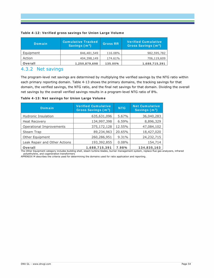
DNV GL – www.dnvgl.com Page 54
Table 4-12: Verified gross savings for Union Large Volume
Domain Cumulative Tracked Savings (m3) Gross RR Verified Cumulative
Gross Savings (m3)
Equipment 846,481,549 116.08% 982,595,782 Action 404,398,149 174.61% 706,119,609 Overall 1,250,879,698 135.00% 1,688,715,391
4.3.2 Net savings The program-level net savings are determined by multiplying the verified savings by the NTG ratio within each primary reporting domain. Table 4-13 shows the primary domains, the tracking savings for that domain, the verified savings, the NTG ratio, and the final net savings for that domain. Dividing the overall net savings by the overall verified savings results in a program-level NTG ratio of 8%.
Table 4-13: Net savings for Union Large Volume
Domain Verified Cumulative Gross Savings (m3) NTG Net Cumulative
Savings (m3)
Hydronic Insulation 635,631,096 5.67% 36,040,283 Heat Recovery 134,997,398 6.59% 8,896,329 Operational Improvements 375,172,128 12.55% 47,084,102 Steam Trap 89,234,963 20.65% 18,427,020 Other Equipment 260,286,951 9.31% 24,232,715 Leak Repair and Other Actions 193,392,855 0.08% 154,714 Overall 1,688,715,391 7.98% 134,835,163
The Other Equipment category includes building shell, steam turbine blades, burner management system, replace flue gas analyzers, infrared polyethylene, and cogeneration transformers
APPENDIX M describes the criteria used for determining the domains used for ratio application and reporting.

DNV GL – www.dnvgl.com Page 55
5 Enbridge Commercial, Industrial, and Multi-Residential Programs
Enbridge’s custom program offerings encourage commercial and industrial customers to reduce their energy consumption by providing financial incentives, technical expertise, and guidance for energy related decision-making. They differ from the prescriptive and direct install programs as they provide services and varying financial incentives based on overall natural gas savings realized by the customer to address customer-specific needs.
There are three programs covered in this section: Enbridge Commercial Custom, Enbridge Industrial Custom Solutions, and Low Income Multi-Residential Affordable Housing.
5.1 Commercial Custom and Industrial Custom Solutions (Enbridge)
The goal of the Enbridge Commercial Custom offer is to reduce natural gas use through the capture of energy efficiency opportunities in commercial buildings, including retrofits of building components and upgrades at the time of replacement.
The Enbridge Industrial Custom Solutions offer is designed to capture energy savings within the industrial sector by supporting customers through a continuous improvement approach. Industrial Energy Solutions Consultants (ESCs) assist customers with the adoption of energy efficient technologies by overcoming financial, knowledge or technical barriers.
A subset of the measures16 in the commercial program is part of the multi-family or multi-residential segment.
All measures implemented as part of these programs and claimed in 2015 are included in the CPSV and FR results in the next sections.
5.2 Low-income Multi-Residential Affordable Housing (Enbridge) This program offers multi-family low-income housing customers incentives to encourage energy efficient upgrades and funding for energy audits. The program also provides technical services, benchmarking, and education for housing providers, building operators, and tenants about their building’s energy usage and ways to achieve energy efficiency. Eligible measures include boilers, ventilation systems, building envelope, window upgrades, in-suite water conservation measures (faucet aerators and showerheads), and heat reflector panels.
The target markets for this program are social and assisted housing providers who own and operate Part 3 buildings and private multi-residential building owners that provide housing to low-income households.17 In addition, Enbridge targets shelters and supportive housing.
16 Throughout the report we will refer to unique combinations of Enbridge project codes and project sub-codes and measures. 17 “Part 3” references buildings covered by Part 3 of the Ontario Building Code, defined as those exceeding 600 square meters in area or greater than
three storeys in height; for residential energy efficiency programs, these are typically multifamily buildings.

DNV GL – www.dnvgl.com Page 56
Custom measures implemented as part of these programs and claimed in 2015 are included in the CPSV results; 4% of the Enbridge low income multi-family (LI MF) program savings are from custom measures. We did not include measures implemented as part of this program in the NTG evaluation.
5.3 CPSV results This section summarizes the gross savings verification (CPSV) energy savings verification results for the Enbridge C&I, MR MF and LIMF Programs. Section 5.3.1 summarizes the data collection efforts, section 5.3.2 presents the gross savings realization rate, and section 5.3.3 summarizes the reasons for the discrepancies between the ex ante and ex post gross savings estimates, and.
5.3.1 Summary of CPSV data collection Table 5-1 summarizes the CPSV data collection efforts for the Enbridge C&I and LIMF Programs. This includes the number of targeted sites and measures that:
Had completed on-site visits Had completed telephone supported engineering reviews (TSER) Did not respond to an evaluation attempt at contact Were not contacted by the evaluation team18
The data collected is represented as the number of sites, the number of measures, the number of units of analysis, and cumulative ex ante natural gas savings. The proportion of the program in each category is also represented in Figure 5-1. The full sample design and achievement by strata can be found in 8. By collecting data on all measures at a site rather than only the first selected, the evaluation exceeded the targeted number of units despite collecting data from fewer sites and TSER units than targeted. The study had a 57% customer response rate and achieved the targeted 90/10 relative precision for the gross realization rate at the overall program level (shown in Table 5-2).
Table 5-1: Summary of CPSV data collection for Enbridge Custom C&I, MF, and LIMF programs*
Data Collection Category
Targeted Completed
# Units of Analysis # Sites #
Measures # Units of Analysis Ex Ante CCM
Completed On-Site 40 37 88 61 250,801,165
Completed TSER 38 31 39 37 81,376,035
Attempted Contact, Not Completed 54 66 65 140,499,585
Not Attempted 584 734 670 401,730,740
Total 706 927 833 874,407,525
* Please see the glossary for definitions of unit of analysis, site, and measure.
18 Sites, projects, or units of analysis where contact was not attempted were either not selected for contact in sampling or in the backup sample and
were not contacted due to strata quotas being met.

DNV GL – www.dnvgl.com Page 57
Figure 5-1: Summary of CPSV data collection for Enbridge Custom C&I and LIMF programs
5.3.2 Gross savings realization rate The gross savings realization rate represents the differences in ex post and ex ante savings due to differences in calculation methods, EUL, calculation parameters, or other engineering-related adjustments. Table 5-2 shows the gross savings realization rate by domain for the Enbridge Custom C&I, MF, and LIMF offerings. The table shows the number of units of analysis (n), gross savings realization rate (Ratio), precision at the 90% confidence interval, error ratio, and percent of program savings. The percent of program savings represents the relative contribution that each domain makes to the overall result.
Enbridge’s C&I and LIMF programs overall had a sample weighted 95% gross realization rate. These domains were found to have variation in engineering adjustment ratios ranging from 87% to 125%. The largest domain for these programs is the combined Custom Commercial and Multi-residential programs, which include all commercial measures as well as all MRMF and LIMF measures. The 91% realization rate is driven by 6 measures with RRs less than 67%. The discrepancies in these measures were mostly due to documentation that did not match what the verifier found onsite, a lack of pre-/post-usage data, differences in billing and simulation results, and EUL changes. The high realization rate for steam traps is primarily due to a change in EUL from 5 years to 6. Relative precision for the programs overall was 9% at 90% confidence.

DNV GL – www.dnvgl.com Page 58
Table 5-2: Gross savings realization rate for Enbridge Custom C&I, and LIMF offerings
Sector Domain n
Ratio 90% Confidence Interval
Error Ratio
% Program Savings Meas Custs +/- Lower
Bound Upper Bound
Relative Precision
Custom Industrial
Heat Recovery 13 10 98% 5% 93% 103% 5% 0.09 9%
Steam Trap 8 8 128% 3% 125% 131% 2% 0.04 2%
Other 32 25 99% 4% 95% 103% 4% 0.11 28% Custom Commercial and LIMF 74 41 91% 14% 78% 105% 15% 0.57 61%
Overall* 127 82 95% 9% 86% 103% 9% 0.51 100% Other industrial: controls, Etools boiler, Etools boiler add-on, Etools insulation, Etools ventilation, other (low temperature spray washer chemical,
increase mechanical dewatering, furnace burner tune-up, infrared heater and programable thermostat, low temp catalytic oxidizer, air curtain, and industrial roll-up doors, water heater)
APPENDIX M describes the criteria used for determining the domains used for ratio application and reporting. Clusters reported in this table are unique customers per stratum: one customer may be in multiple strata, so the count of clusters is greater than the
number of customers contacted. *Overall ratio in this table is the sample weighted average and is not used in calculating gross savings for the programs.
Figure 5-2 also shows the gross savings realization rate by domain. The figure shows the ratio point estimate as a blue dot on the horizontal axis and the confidence interval as hashmarks connected by a green line. The number of units of analysis, the numeric ratio, and the percent of program savings represented by each domain are shown to the right of the plot.
Figure 5-2: Engineering adjustment for Enbridge Custom C&I, MF, and LIMF programs

DNV GL – www.dnvgl.com Page 59
5.3.3 Discrepancy summary This section presents detailed results for the reasons for and magnitude of the various discrepancies between ex ante and ex-post savings. First we will look at the cumulative savings, then the two key components of cumulative savings: annual savings and the EUL. See APPENDIX Q for additional detail.
Figure 5-3 plots the ex post cumulative savings against the ex ante cumulative savings for each measure in the sample. The plot on the left shows the full set of measures, while the plot on the right is focused in on the cluster of measures with less than 10 million CCM in both ex ante and ex post. The diagonal line represents a 100% engineering adjustment, or the plotted value if ex post equals ex ante. Points above the line indicate measures where ex post savings were greater than ex ante, while points below the line indicate where ex post were less than ex ante.
Most measures had similar ex post and ex ante savings. Heat recovery measures tended to have the largest adjustments. Two heat recovery measures resulted in large negative discrepancies, the largest of which was due to the site contact providing updated measured gas use. Two other large heat recovery measures had positive adjustments (each due to different operating conditions for found in the ex post verification.
Figure 5-3: Ex post versus ex ante cumulative savings (CCM) - Enbridge C&I and MF, by measure type
5.3.3.1 First-year savings discrepancies Figure 5-4 plots the ex post annual savings against the ex ante annual savings for each measure in the sample. The plot on the left shows the full set of measures, while the plot on the right is focused in on the cluster of measures with less than 0.20 million m3 in both ex ante and ex post. The diagonal line represents a 100% engineering adjustment, or the plotted value if ex post equals ex ante. Points above the line
Zoom in on <=10 million CCM

DNV GL – www.dnvgl.com Page 60
indicate measures where ex post savings were greater than ex ante, while points below the line indicate where ex post were less than ex ante.
Like the cumulative savings, most measures had similar ex post and ex ante savings. At the high level the pattern is consistent in terms of types of measures with large adjustment.
Figure 5-4. Ex post versus ex ante annual savings - Enbridge C&I and MF, by measure type
5.3.3.2 Measure life discrepancies One of the primary discrepancies is a change in EUL between ex ante and ex post. Figure 5-5 plots the ex post EUL against the ex ante EUL for each measure in the sample. Because EULs tend to be discrete numbers, the size of the bubbles in the plot indicate show the relative amount of ex ante savings for the measures at each plotted point (e.g., the larger the bubble, the more savings at that point). The diagonal line represents the plotted value if ex post equals ex ante. Points above the line indicate measures where ex post EUL were greater than ex ante, while points below the line indicate where ex post were less than ex ante.
The plot shows that most savings had equal ex post and ex ante EULs. The greatest differences represented relatively small savings.
Figure 5-5: Ex post versus ex ante effective useful life - Enbridge C&I and MF
Zoom in on <=0.20 million

DNV GL – www.dnvgl.com Page 61
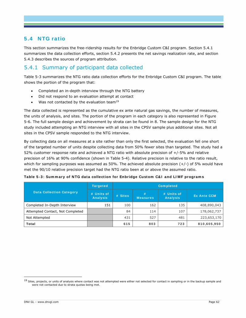
DNV GL – www.dnvgl.com Page 62
5.4 NTG ratio This section summarizes the free-ridership results for the Enbridge Custom C&I program. Section 5.4.1 summarizes the data collection efforts, section 5.4.2 presents the net savings realization rate, and section 5.4.3 describes the sources of program attribution.
5.4.1 Summary of participant data collected Table 5-3 summarizes the NTG ratio data collection efforts for the Enbridge Custom C&I program. The table shows the portion of the program that:
Completed an in-depth interview through the NTG battery Did not respond to an evaluation attempt at contact Was not contacted by the evaluation team19
The data collected is represented as the cumulative ex ante natural gas savings, the number of measures, the units of analysis, and sites. The portion of the program in each category is also represented in Figure 5-6. The full sample design and achievement by strata can be found in 8. The sample design for the NTG study included attempting an NTG interview with all sites in the CPSV sample plus additional sites. Not all sites in the CPSV sample responded to the NTG interview.
By collecting data on all measures at a site rather than only the first selected, the evaluation fell one short of the targeted number of units despite collecting data from 50% fewer sites than targeted. The study had a 52% customer response rate and achieved a NTG ratio with absolute precision of +/-5% and relative precision of 16% at 90% confidence (shown in Table 5-4). Relative precision is relative to the ratio result, which for sampling purposes was assumed as 50%. The achieved absolute precision (+/-) of 5% would have met the 90/10 relative precision target had the NTG ratio been at or above the assumed ratio.
Table 5-3: Summary of NTG data collection for Enbridge Custom C&I and LIMF programs
Data Collection Category
Targeted Completed
# Units of Analysis # Sites #
Measures # Units of Analysis Ex Ante CCM
Completed In-Depth Interview 151 100 162 135 408,890,043
Attempted Contact, Not Completed 84 114 107 178,062,737
Not Attempted 431 527 481 223,653,170
Total 615 803 723 810,605,950
19 Sites, projects, or units of analysis where contact was not attempted were either not selected for contact in sampling or in the backup sample and
were not contacted due to strata quotas being met.

DNV GL – www.dnvgl.com Page 63
Figure 5-6: Summary of NTG data collection for Enbridge Custom C&I programs
5.4.2 Free-ridership Free-ridership is the sole contributor to the NTG ratio. The evaluation team is also conducting a study of the spillover savings attributable to the program; those results will be presented in a later report. The free-ridership is calculated from self-reported responses to survey questions as outlined in APPENDIX J.
Table 5-4 shows the NTG ratio by domain for the Enbridge Custom C&I programs. The table shows the number of units of analysis (n), NTG ratio (Ratio), precision at the 90% confidence interval, error ratio, and percent of program savings. The percent of program savings represents the relative contribution that each domain makes to the overall result.
Enbridge’s C&I programs overall had 29% attribution, or 71% free-ridership. Ventilation measures showed the lowest attribution (4-19% in each sector) while multi-residential other (non-boiler, non-ventilation) showed the highest attribution at 97%. Industrial Heat Recovery measures were the only other domain over 50% attribution at 56%.

DNV GL – www.dnvgl.com Page 64
Table 5-4: NTG ratio for Enbridge Custom C&I programs
Sector Domain n
NTG Ratio
90% Confidence Interval Error Ratio
% Program Savings
Meas. Custs. +/- Lower Bound
Upper Bound
Relative Precision
Custom Industrial
Etools Ventilation 8 7 15% 10% 5% 25% 70% 0.95 10%
Heat Recovery 13 10 55% 9% 46% 64% 16% 0.27 10%
Other 39 34 31% 7% 24% 38% 24% 0.81 22%
Custom Commercial
Etools Boiler and Boiler Add-on
25 20 24% 11% 13% 35% 47% 1.22 12%
Etools Ventilation 15 15 5% 4% 1% 8% 72% 1.58 8%
Steam Trap 14 6 27% 5% 22% 33% 19% 0.23 2%
Other 12 8 18% 14% 4% 32% 76% 1.14 16%
Custom Multi-Residential
Etools Boiler 11 8 26% 14% 12% 40% 54% 0.80 13% Etools Ventilation 7 7 20% 14% 6% 34% 71% 0.97 3%
Other 17 7 97% 3% 94% 100% 3% 0.05 3%
Overall* 161 112 29% 4% 25% 34% 15% 0.97 100% Other Industrial: Controls, Etools boiler, Etools boiler add-on, Etools insulation, steam trap, other (increase mechanical dewatering, VFD, infrared
heater and programmable thermostat, low temp catalytic oxidizer, air curtain, industrial roll-up doors, evaporator system, water heater, reduce powder paint curing oven exhaust, dock seal, aquathermat heating system, insulated panels, greenhouse double polyethylene walls)
Other Commercial: Etools insulation, controls, other (dock seal, building shell, steam chiller, high speed door, boiler – hydronic high-efficiency) Other Multi-res: Etools boiler add-on, Etools insulation, heat reflector panels APPENDIX M describes the criteria used for determining the domains used for ratio application and reporting. Clusters reported in this table are unique customers per stratum: one customer may be in multiple strata, so the count of clusters is greater than the
number of customers contacted. *Overall ratio in this table is the sample weighted average and is not used in calculating net savings for the programs.
Figure 5-7 also shows the NTG ratio by domain. The figure shows the ratio point estimate as a blue dot on the horizontal axis and the confidence interval as hashmarks connected by a green line. The number of units of analysis, the numeric ratio, and the percent of program savings represented by each domain are shown to the right of the plot.

DNV GL – www.dnvgl.com Page 65
Figure 5-7: NTG ratio for Enbridge Custom C&I programs
5.4.3 Sources of attribution As outlined in APPENDIX K, the NTG ratio is an estimate of a program’s influence on the timing, quantity, and efficiency of the measure installed. This section details the program’s effect on each of those sources of attribution and indicates where the program is creating the greatest transformation.
Table 5-5 represents the possible combinations of timing, efficiency, and quantity attribution. A “yes” in the timing, efficiency, or quantity column indicates partial or full attribution for that source. A “no” indicates no attribution for that source. For example, the row that has Yes for timing, efficiency, and quantity reports the portion of the program that indicated that the program had at least partial influence on the timing, efficiency, and quantity for that measure. For some measures, efficiency or quantity may not be applicable questions; for the purposes of this table, the not applicable measures are included as “no” on the non-applicable dimension.
The table also shows the portion of the program that falls into each combination of timing, efficiency, and quantity attribution represented by the number of responses and the percent of cumulative savings represented by that category.
The table shows that approximately two-thirds (63%) of program savings were at least partially influenced by the program. Of the three aspects relating to savings that the program can influence, timing is the most common, affecting approximately 57% of the program savings. Quantity affects approximately 20% of the

DNV GL – www.dnvgl.com Page 66
program savings, and the program influenced efficiency levels of equipment accounting for approximately 13% of program savings.
Table 5-5. Overview of the sources of attribution for Enbridge Custom C&I programs
Attribution
Timing Efficiency Quantity Customers* Units of Analysis Measures Percent
Savings Yes Yes Yes 0 0 0 0% Yes Yes No 7 8 8 8% Yes No Yes 18 27 33 20% Yes No No 28 34 49 30% No Yes Yes * * * <1% No Yes No * 5 5 6% No No Yes 5 5 5 <1% No No No 42 54 60 36%
For confidentiality reasons the numbers of customers, units of analysis and measures less than 5 are not displayed. A customer may appear multiple times if their responses varied by measures, resulting in a total greater than the number of customers interviewed.
5.4.3.1 Timing component Respondents answered a sequence of questions that addresses the timing of the equipment installation. First, respondents answered the likelihood of installing the same type of equipment at the same time without the program (DAT1a). Respondents who answered “Later” specified the number of months later in the next question (DAT1b). 20
Timing was the component most strongly affected by the program. The program affected the timing of measures that account for more than half of program savings. Forty-eight out of 100 surveyed customers accounting for 43% of program savings said they would have installed their measure(s) at the same time. The rest indicated some amount of program acceleration, mostly between 1 and 48 months (Table 5-6).
Table 5-6. Determining the Acceleration period, Enbridge Custom C&I programs
DAT1a. Without the utility, how different would the timing have been? DAT1b. Approximately how many months later?
DAT1a DAT1b
Customers*
Units of Analysis
Measures
Percent Saving
s Timing Attribution Same Time N/A 48 66 72 43% 0% Earlier N/A 0 0 0 0% 0%
Later
Months < 48 33 44 59 35% ER baseline credit**
for months accelerated
Months ≥ 48 * * * 1% 100%+ ER baseline credit
Don't Know/ Refused 5 5 5 2% ER baseline credit for
avg. of DAT1b Never N/A 9 15 21 14% 100% Don't Know/ Refused N/A * * * 0% ER baseline credit for
avg. of DAT1a
20 See APPENDIX K for the detailed scoring algorithm.

DNV GL – www.dnvgl.com Page 67
For confidentiality reasons the numbers of customers, units of analysis and measures less than 5 are not displayed. *A customer may appear multiple times if their responses varied by measures, resulting in a total greater than the number of customers interviewed. **ER baseline credit reflects credit for a vs. in situ equipment baseline savings during the acceleration period.
5.4.3.2 Efficiency Component Respondents answered a sequence of questions that addresses the program’s effects on the efficiency level of the installed equipment. First, respondents indicated the likelihood of installing the same level of efficiency without the program (DAT2a). Respondents who answered that they would have installed a less efficient option answered a follow-up question (DAT2b) to specify the level of efficiency they would have installed.
The program had limited effect on efficiency (Table 5-7). Most (54%) of program savings were from measures for which efficiency levels is not applicable such as operational improvements, leak repairs or steam trap replacements. Most of the remaining survey respondents said the program had no effect on the efficiency level of the equipment installed. Respondents who indicated the program increased the efficiency level of their measures accounted for approximately 13% of program savings. Most of these indicated that the program moved them from an efficiency level already above standard efficiency to an even higher level of efficiency. The relatively low program influence on efficiency can be an indicator that measures included in the program, though above current code requirements, are standard on the market.
Table 5-7. Determining Efficiency Attribution, Enbridge Custom C&I programs
DAT2a. Without the utility, would you have installed the same, higher, or lower efficiency? DAT2b. Without the utility, what efficiency would you have installed?
DAT2a DAT2b Customers*
Units of Analysis
Measures
Percent Savings
Efficiency Attribution
Same N/A/Skipped 31 37 41 33% 0%
Lower
Standard Efficiency * * * <1% 100% Between Standard and High 6 6 6 10% 50%
Don't Know/Refused 5 6 6 3% Average of DAT2b
Higher N/A/Skipped 0 0 0 0% 0% Don't Know/Refused N/A Skipped * * * <1% Average of
DAT2a Not Applicable N/A 57 83 106 54% Not Asked
For confidentiality reasons the numbers of customers, units of analysis and measures less than 5 are not displayed. A customer may appear multiple times if their responses varied by measures, resulting in a total greater than the number of customers interviewed.
5.4.3.3 Quantity Component Respondents answered a sequence of questions that addresses the program’s effects on the amount of equipment installed. First, respondents indicated the likelihood of installing the same amount of equipment (or capacity for measures for which number is not relevant, such as heat exchangers) without the program (DAT3a). Respondents who answered that they would have installed less or more equipment answered a follow-up question (DAT3b) to specify how the program changed the amount that they installed.
The program had limited effect on the quantity of measures installed. Sixty-five of the 96 customers, who accounted for 82% of program savings, said they would have purchased the same amount of equipment

DNV GL – www.dnvgl.com Page 68
without the program (Table 5-8). Most of the remaining customers (12% of savings) received full attribution because they indicated they would not have installed any measures without the program.
Table 5-8. Determining quantity/size attribution, Enbridge Custom C&I programs
DAT3a. Without the utility, how different would the quantity/size have been? DAT3b. By what percentage did you change the amount installed because of utility?
DAT3a DAT3b Customers* Units of Analysis Measures Percent
Savings Quantity
Attribution
Same N/A 65 94 117 82% 0%
Less
Value < 100% 9 11 11 4% Value < 50% Value ≥ 100% * * * <1% Value > 50% Don't Know/Refused * * * <1% Average of
DAT3a
More
Value < 100% 0 0 0 0% Value < 100%
Value ≥ 100% 0 0 0 0% Value = 100%
Don't Know/ Refused 0 0 0 0% Average of
DAT3a None N/A 10 16 19 11% 100% Don't Know/ Refused N/A * * * <1% Average of
DAT3 Not Applicable N/A 7 9 10 2% Not Asked
For confidentiality reasons the numbers of customers, units of analysis and measures less than 5 are not displayed. A customer may appear multiple times if their responses varied by measures, resulting in a total greater than the number of customers interviewed.
5.5 Gross and net savings This section reports the evaluation-verified gross savings in section 5.5.1 and the net savings (including only free-ridership) in section 5.5.2.
5.5.1 Verified gross savings Program-level gross savings are determined by multiplying the tracking savings by the gross realization rate within each primary reporting domain. Table 5-9 shows the primary domains, the tracking savings for that domain, the gross realization rate, and the final verified gross savings for that domain. Dividing the overall verified gross savings by the overall tracking savings results in a program-level gross realization rate of 92%.
Table 5-9: Verified gross savings for Enbridge Custom C&I and LIMF programs
Sector Applied Domain Cumulative Tracked Savings (m3)
Gross RR
Verified Cumulative Gross
Savings (m3)
Custom Industrial
Heat Recovery 82,143,555 97.86% 80,385,683 Steam Trap 20,222,930 127.62% 25,808,503 Other 241,990,817 98.78% 239,038,529 Total 344,357,302 100.25% 345,232,715
Custom Commercial and Multi-Residential 466,248,648 91.48% 426,524,263 Low Income Multi-Residential 63,801,575 91.48% 58,365,681

DNV GL – www.dnvgl.com Page 69
5.5.2 Net savings Program-level net savings are determined by multiplying the verified gross savings by the NTG ratio within each primary reporting domain. Table 5-10 shows the primary domains, tracking savings, verified savings, NTG ratio, and the final net savings for that domain.
Table 5-10: Net savings for Enbridge Custom C&I programs
Sector Applied Domain Verified
Cumulative Gross Savings (m3)
NTG Net
Cumulative Savings (m3)
Custom Industrial
Etool Ventilation 83,670,201 14.90% 12,466,860 Heat Recovery 80,385,683 55.25% 44,413,090 Other 181,176,831 31.04% 56,237,288 Total 345,232,715 32.77% 113,117,238
Custom Commercial
Etool Boiler and Boiler Add-on 90,295,668 24.09% 21,752,226 Etool Ventilation 61,235,559 4.93% 3,018,913 Steam Trap 13,597,779 27.42% 3,728,511 Other 121,290,363 18.22% 22,099,104 Total 286,419,369 17.67% 50,598,755
Market Rate Multi-Residential
Etool Boiler 98,725,211 26.18% 25,846,260 Etool Ventilation 21,825,719 19.70% 4,299,667 Other 19,553,964 97.10% 18,986,899 Total 140,104,894 35.07% 49,132,826
Low Income Multi-Residential* 58,365,681 100.00% 58,365,681 The Other Industrial category includes: Controls, Etools boiler, Etools boiler add-on, Etools insulation, steam trap, other (increase mechanical
dewatering, VFD, infrared heater and programmable thermostat, low temp catalytic oxidizer, air curtain, industrial roll-up doors, evaporator system, water heater, reduce powder paint curing oven exhaust, dock seal, aquathermal heating system, insulated panels, and greenhouse double polyethylene walls)
The Other Commercial category includes: Etools insulation, controls, other (dock seal, building shell, steam chiller, high speed door, boiler – hydronic high-efficiency)
The Other Multi-residential category includes: Etools boiler add-on, Etools insulation, and heat reflector panels. *The Enbridge Low Income Multi-Residential NTG ratio is deemed at 100%.
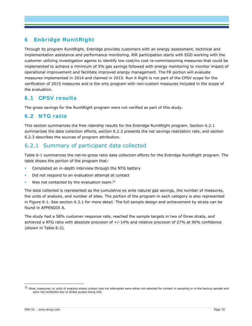
DNV GL – www.dnvgl.com Page 70
6 Enbridge RunitRight Through its program RunitRight, Enbridge provides customers with an energy assessment, technical and implementation assistance and performance monitoring. RiR participation starts with EGD working with the customer utilizing investigation agents to identify low cost/no cost re-commissioning measures that could be implemented to achieve a minimum of 5% gas savings followed with energy monitoring to monitor impact of operational improvement and facilitate improved energy management. The FR portion will evaluate measures implemented in 2014 and claimed in 2015. Run it Right is not part of the CPSV scope for the verification of 2015 measures and is the only program with non-custom measures included in the scope of the evaluation.
6.1 CPSV results The gross savings for the RunitRight program were not verified as part of this study.
6.2 NTG ratio This section summarizes the free ridership results for the Enbridge RunitRight program. Section 6.2.1 summarizes the data collection efforts, section 6.2.2 presents the net savings realization rate, and section 6.2.3 describes the sources of program attribution.
6.2.1 Summary of participant data collected Table 6-1 summarizes the net-to-gross ratio data collection efforts for the Enbridge RunitRight program. The table shows the portion of the program that:
Completed an in-depth interview through the NTG battery
Did not respond to an evaluation attempt at contact
Was not contacted by the evaluation team.21
The data collected is represented as the cumulative ex ante natural gas savings, the number of measures, the units of analysis, and number of sites. The portion of the program in each category is also represented in Figure 6-1. See section 6.3.1 for more detail. The full sample design and achievement by strata can be found in APPENDIX A.
The study had a 58% customer response rate, reached the sample targets in two of three strata, and achieved a NTG ratio with absolute precision of +/-14% and relative precision of 27% at 90% confidence (shown in Table 6-2).
21 Sites, measures, or units of analysis where contact was not attempted were either not selected for contact in sampling or in the backup sample and
were not contacted due to strata quotas being met.
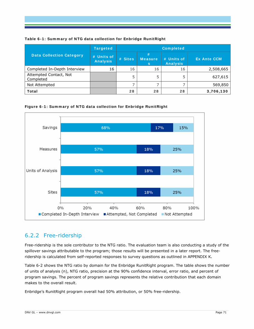
DNV GL – www.dnvgl.com Page 71
Table 6-1: Summary of NTG data collection for Enbridge RunitRight
Data Collection Category
Targeted Completed
# Units of Analysis # Sites
# Measure
s
# Units of Analysis
Ex Ante CCM
Completed In-Depth Interview 16 16 16 16 2,508,665 Attempted Contact, Not Completed 5 5 5 627,615
Not Attempted 7 7 7 569,850
Total 28 28 28 3,706,130
Figure 6-1: Summary of NTG data collection for Enbridge RunitRight
6.2.2 Free-ridership Free-ridership is the sole contributor to the NTG ratio. The evaluation team is also conducting a study of the spillover savings attributable to the program; those results will be presented in a later report. The free-ridership is calculated from self-reported responses to survey questions as outlined in APPENDIX K.
Table 6-2 shows the NTG ratio by domain for the Enbridge RunitRight program. The table shows the number of units of analysis (n), NTG ratio, precision at the 90% confidence interval, error ratio, and percent of program savings. The percent of program savings represents the relative contribution that each domain makes to the overall result.
Enbridge’s RunitRight program overall had 50% attribution, or 50% free-ridership.

DNV GL – www.dnvgl.com Page 72
Table 6-2: NTG ratio for Enbridge RunitRight
Domain n
Ratio 90% Confidence Interval Error
Ratio
% Program Savings Measures Customers +/- Lower
Bound Upper Bound
Relative Precision
RunitRight 16 10 50% 14% 36% 64% 27% 0.47 100% APPENDIX M describes the criteria used for determining the domains used for ratio application and reporting. Clusters reported in this table are unique customers per stratum: one customer may be in multiple strata, so the count of clusters is greater than the
number of customers contacted.
Figure 6-2 also shows the NTG ratio for this program. The figure shows the ratio point estimate as a blue dot on the horizontal axis and the confidence interval as hashmarks connected by a green line. The number of units of analysis, numeric ratio, and percent of program savings represented by each domain are shown to the right of the plot. Attribution for the RunitRight program is higher than most of Enbridge’s custom offerings, with the exceptions of Heat Recovery and Multi-Residential Other.
Figure 6-2: NTG ratio for Enbridge RunitRight
6.2.3 Sources of attribution As outlined in APPENDIX K, the NTG ratio is a combination of responses regarding the program’s influence on the timing, quantity, and efficiency of the measure implemented. Since most measures in the RunitRight program are a result of low cost/no cost operational improvements and re-commissioning which does not have its own inherent efficiency, the efficiency question was not asked for the participants of this program.

DNV GL – www.dnvgl.com Page 73
This section details the program’s effect on each of those sources of attribution and indicates where the program is creating the greatest transformation.
Table 6-3 represents the possible combinations of timing and quantity attribution. A “yes” in the timing or quantity column indicates partial or full attribution for that source. A “no” indicates no attribution for that source. For example, the row that has Yes for timing and quantity reports the portion of the program that indicated that the program had at least partial influence on the timing and quantity for that measure.
The table also shows the number of customers, measures, and savings that fall into each combination. The portion of the program that falls into each combination of timing and quantity attribution is represented by the number of responses and the percent of cumulative savings represented by that category.
The table shows that all program participation was at least partially influenced by the program. The program affected the timing of all measures. It had a limited effect on quantity, influencing measures that accounted for approximately 7% of program savings.
Table 6-3. Overview of the sources of attribution for Enbridge RunitRight
Attribution
Timing Quantity Customers* Units of Analysis Measures Percent
Savings Yes Yes * * * 7% Yes No 6 15 15 93% No Yes 0 0 0 0% No No 0 0 0 0%
A * refers to a category with fewer than 5 participants. These are not shown for customer privacy reasons. A customer may appear multiple times if their responses varied by measures, resulting in a total greater than the number of customers interviewed.

DNV GL – www.dnvgl.com Page 74
6.2.3.1 Timing component Respondents answered a sequence of questions that addresses the timing of the energy saving activities. First, respondents answered the likelihood of performing the energy saving activities at the same time without the program (DAT1a). Respondents who answered “Later” specified the number of months later in the next question (DAT1b). 22
Timing was the component most strongly affected by the program. No customers indicated they would have completed the energy saving activities at the same time. Customers indicated that measures accounting for over a quarter of savings would not have been completed for four or more years and measures accounting for nearly an additional 59% of savings would have been completed within four years. The rest indicated that they didn’t know when the measure would have been completed or refused to answer the question (Table 6-4).
Table 6-4. Determining the Acceleration period, Enbridge RunitRight
DAT1a. Without the utility, how different would the timing have been? DAT1b. Approximately how many months later?
DAT1a DAT1b Customers* Units of Analysis Measures Percent
Savings Timing
Attribution Same Time N/A 0 0 0 0% 0% Earlier N/A 0 0 0 0% 0%
Later
Months < 48 * 7 7 59% ER baseline**
credit for months accelerated
Months ≥ 48 * 6 6 26% 100%+ ER baseline credit
Don't Know/ Refused * * * 7%
ER baseline credit for avg. of
DAT1b Never N/A 0 0 0 0% 100%
Don't Know/ Refused N/A * * * 9%
ER baseline credit for avg. of
DAT1a For confidentiality reasons the numbers of customers, units of analysis and measures less than 5 are not displayed. *A customer may appear multiple times if their responses varied by measures, resulting in a total greater than the number of customers interviewed. **ER baseline credit reflects credit for a vs. in situ equipment baseline savings during the acceleration period.
6.2.3.2 Quantity Component Respondents answered a sequence of questions that addresses the program’s effects on the extent of energy savings activities taken. First, respondents answered the likelihood of performing the same amount of energy saving activities without the program (DAT3a). Respondents who answered that they would have done more answered a follow-up question (DAT3b) to specify how the program changed the amount of activity that they performed.
The program had a small effect on quantity. Respondents indicated that they would have performed the same amount of activity in measures that accounted for almost all (93%) of the program savings. For confidentiality reasons this table is not provided.
22 See APPENDIX K for the detailed scoring algorithm.

DNV GL – www.dnvgl.com Page 75
6.3 Gross and net savings The RunitRight program was not included in the CPSV portion of the study. This section reports the net savings (including only free-ridership) in section 6.3.1.
6.3.1 Net savings The program-level net savings are determined by multiplying the verified savings by the NTG ratio within each primary reporting domain. Table 6-5 shows the tracking savings, NTG ratio, and final net savings. Dividing the overall net savings by the overall verified savings results in a program-level NTG ratio of 50%.
Table 6-5: Net savings for Enbridge RunitRight
Domain Cumulative Tracking Savings (m3) NTG Net Cumulative
Savings (m3)
RunitRight 2,712,210 50.06% 1,357,732

DNV GL – www.dnvgl.com Page 76
7 Findings and recommendations In the tables the primary outcomes of the recommendation are classified into four categories: reduce costs, increase savings, increase (or maintain) customer satisfaction and decrease risk (multiple types of risk are in this category including risk of adjusted savings, risk to budgets or project schedules, and others). Details of the findings, recommendations and outcomes follow the tables.
Table 7-1: Energy savings and program performance recommendations
#
Energy Savings and Program
Performance
Recommendation
Applies to Primary Outcome
Un
ion
Enb
rid
ge
Eval
uat
ion
Red
uce
Cos
ts
Incr
ease
Sav
ing
s
Incr
ease
Cu
sto
mer
Sat
isfa
ctio
n
Dec
reas
e
Ris
k
ES1 The utilities should continue in their
commitment to accuracy.
ES2 Evaluate free-ridership for the programs
annually and couple the free-ridership
evaluation with process evaluation
ES3 Error ratios from this report inform sample
design for future evaluation.
ES4 Align the program design with cumulative net
goals
ES5 Do not pay incentives until after installation is
complete.
ES6 Develop policies to collaborate across electric
and gas projects to avoid double-counting fuel
savings and increases from energy efficiency
measures.
ES7 Consider establishing a policy to define rules
around energy savings calculation for fuel
switching and district heating/cooling
measures.
ES8 Consider establishing a policy that defines an
eligibility floor and cap based on simple
payback period for energy efficiency projects.
ES9 Consider establishing an official definition for
EUL and implementing a study to define EULs
for program measures

DNV GL – www.dnvgl.com Page 77
#
Energy Savings and Program
Performance
Recommendation
Applies to Primary Outcome
Un
ion
Enb
rid
ge
Eval
uat
ion
Red
uce
Cos
ts
Incr
ease
Sav
ing
s
Incr
ease
Cu
sto
mer
Sat
isfa
ctio
n
Dec
reas
e
Ris
k
ES10 Track metrics for how long it takes from the
final installation verification to the posting of
incentive payments.
ES11 Increase transparency of “influence
adjustments” and do not include in gross
savings
ES12 Conduct a process evaluation to improve
Large Volume influence on customer projects
ES13 Consider approaches to market that leverage
third-party vendors.
Table 7-2: Verification process recommendations
#
Verification Process
Recommendation
Applies to Primary Outcome
Un
ion
Enb
rid
ge
Eval
uat
ion
Red
uce
Cos
ts
Incr
ease
Sav
ing
s
Incr
ease
Cu
sto
mer
Sat
isfa
ctio
n
Dec
reas
e
Ris
k
VP1 Modify contracts to require participants to
agree to comply with EM&V as well as utility
representatives as part of the requirements
for participation in the program.
VP2 The verification and utility staff should agree
to a code of conduct for each role during
onsite visits.

DNV GL – www.dnvgl.com Page 78
Table 7-3: Documentation and Support recommendations
#
Documentation and Support
Recommendation
Applies to Primary Outcome
Un
ion
Enb
rid
ge
Eval
uat
ion
Red
uce
Cos
ts
Incr
ease
Sav
ing
s
Incr
ease
Cu
sto
mer
Sat
isfa
ctio
n
Dec
reas
e
Ris
k
DS1 Take steps to improve documentation:
Include explicit sources for all inputs and
assumptions in the project
documentation.
Store background studies and information
sources with the project files and make
them available to evaluators.
Provide evaluators full access to customer
data.
Provide pre- and post-installation photos,
where available.
Document and provide internal M&V
documents where available.
Institute a checklist as part of project
closeout to ensure all relevant project
documentation is assembled as ready for
verification
DS2 Ensure that incremental costs are supported
by invoices or other documentation
DS3 Increase the amount of documentation and
source material for projects that have greater
energy savings.
DS4
A
Digitize and file project documentation for all
projects as they are completed and paid
during project closeout.
DS4
B
Until the utilities can implement an effective
digital document storage process, the
evaluation should allow more time for the
utilities to assemble and deliver the
documentation.

DNV GL – www.dnvgl.com Page 79
#
Documentation and Support
Recommendation
Applies to Primary Outcome
Un
ion
Enb
rid
ge
Eval
uat
ion
Red
uce
Cos
ts
Incr
ease
Sav
ing
s
Incr
ease
Cu
sto
mer
Sat
isfa
ctio
n
Dec
reas
e
Ris
k
DS5 Consider providing more training or adding
quality control steps to ensure the summary
workbook front page is completed and stored
in a consistent manner.
DS6 Use a consistent summary workbook.
Table 7-4: Data management recommendations
#
Data Management
Recommendation
Applies to Primary Outcome
Un
ion
Enb
rid
ge
Eval
uat
ion
Red
uce
Cos
ts
Incr
ease
Sav
ing
s
Incr
ease
Cu
sto
mer
Sat
isfa
ctio
n
Dec
reas
e
Ris
k
DM1
A
Track contacts associated with projects in the
program tracking database.
DM1
B
Strongly consider investing in relational
program tracking databases.
DM1
C
Include structure for improved data integrity
in the evaluator request for contact
information for the 2016 and 2017 savings
verification and evaluation.
DM2
A
Consider offering bonus incentives early in the
year to combat the “hockey stick”
phenomenon where a large percent of
projects get closed in the fourth quarter of the
year (which results in rushed QC for data).
DM3 Track and provide to evaluators dates for key
milestones in the project.
DM4 Maintain a customer identifier in the database
to clearly identify related sites.

DNV GL – www.dnvgl.com Page 80
#
Data Management
Recommendation
Applies to Primary Outcome
Un
ion
Enb
rid
ge
Eval
uat
ion
Red
uce
Cos
ts
Incr
ease
Sav
ing
s
Incr
ease
Cu
sto
mer
Sat
isfa
ctio
n
Dec
reas
e
Ris
k
DM5 Include EUL (also remaining useful life for
dual baselines), NTG, and each of the key
savings types (i.e., annual and cumulative,
gross and net) in the program tracking
extracts provided to evaluators.
Figure 1-1 shows an approximate cost vs. impact relation ship for each of the recommendations on a 4-point scale. The upper left quadrant of the figure shows the recommendations that are relatively low cost that would have a high impact. Those in the upper right are recommendations where both cost and impact are high.
Figure 7-1: Approximate Cost vs. Impact of each recommendation

DNV GL – www.dnvgl.com Page 81
7.1 Energy savings and program performance ES1. Finding: Both utilities exhibit a strong commitment to accurate energy savings estimates. Both
utilities have made significant investments in developing calculation tools which model savings accurately. For example, Union’s dock door seal calculator is well considered and designed, and Enbridge’s Etools calculator is very thorough in attempting to model savings for key measures.
Both utilities chose to retain engineers with strong understandings of their customers’ building and process systems. We had numerous opportunities to interact with these engineers on phone calls and site visits, and have grown to respect their knowledge and engagement with the types of systems that matter to their customers.
Both utilities showed a commitment to finding accurate savings. On several occasions, both on the phone and in writing, the evaluation team suggested a value that would have increased savings in a way that the program engineer did not think was valid. When this happened, neither utility was shy in suggesting that we may want to make a more conservative choice.
Recommendation: The utilities should continue in their commitment to accuracy.
Outcome: Accurate energy savings.
ES2. Finding: Free-ridership in the utilities’ programs is high
Recommendation: With high free-ridership and rapidly changing programs, consistent evaluation of free-ridership annually and free-ridership evaluation coupled with process evaluation will help identify specific ways for each program to manage and reduce free-ridership.
Outcome: Effective free-ridership management will allow the programs to increase their net savings significantly in future years.
ES3. Finding: Relative precision targets were exceeded for some programs and not met for others.
Recommendation: Error ratios from the results provided in this report should be used to inform sample design for future evaluation years.
Outcome: Better defined error ratios for the measures in the programs will allow more efficient sample design for future evaluations, improving precisions and reducing costs.
ES4. Finding: Attribution for the programs came primarily through acceleration rather than changes in efficiency or quantity/size. This is partly due to the measures that dominate the programs: controls, maintenance, and optimisation. These measures do not have varying efficiencies, so the programs are either affecting the number of units implemented or accelerating the measure. Acceleration is less valuable to programs that are seeking to meet cumulative net goals. Acceleration periods tend to be considerably shorter than the estimated useful life (EUL) of a measure and thus the partial attribution that results is low relative to cumulative gross savings.
Recommendation: To align the programs with cumulative net goals, the utilities should seek to:
continue promoting long life measures and consider discontinuing promotion of short lived measures proactively upsell equipment purchases from standard to efficient products target hard to reach customers who have not participated in the past promote EE measures with low market penetration (such as heat reflector panels)

DNV GL – www.dnvgl.com Page 82
motivate customers to increase the scope of their projects, some options include multi-measure bonuses or escalating incentive structures that pay more for doing more
Outcome 1: Focusing on proactive sales rather than reactive will help the net-to-gross (NTG) ratio.
Outcome 2: Effective free-ridership management will allow the program to increase net savings significantly in future years.
ES5. Finding: A handful (<5) of respondents indicated that all or part of their incentivized project had not yet been installed over a year after the incentive was paid.
Recommendation: Do not pay incentives until after installation is complete.
Outcome: Cost-effectiveness of the program will increase as it avoids paying for savings that do not materialize.
ES6. Finding: Some customers receive incentives from their electric provider and natural gas utility to complete the same EE measure. Both providers may claim the same changes in energy use, resulting in overlap when aggregated across fuels at the provincial level.
Recommendation: Develop policies to collaborate across electric and gas projects to avoid double-counting fuel savings and increases from energy efficiency measures.
Outcome: More accurate energy and carbon savings estimates across the province.
ES7. Finding: Some measures (e.g., geothermal heat pumps, combined heat and power, and those that save district heating energy) have difficult-to-define baseline technologies.
Recommendation: Consider establishing a policy to define rules around energy savings calculation for fuel switching and district heating/cooling measures.
Outcome: Less evaluation risk and a better alignment between province energy efficiency goals and program implementation.
ES8. Finding: Projects with very long and very short simple payback periods often have low NTG ratios. However, from a customer service standpoint, it may be difficult for utilities to deny incentives to customers unless they have pre-established rules to point to.
Recommendation: Consider establishing a policy that defines an eligibility floor and cap based on simple payback period for energy efficiency projects.
Outcome: The rule will give utilities a guideline to restrict the program to projects that are more likely to result in net savings. It will also allow the utilities to reject potentially poor projects without a large effect on customer satisfaction.
ES9. Finding: Members of the EAC and evaluation team have different understandings of the definition of some evaluation inputs.
Recommendation: Consider establishing an official definition for EUL and implementing a study to define EUL for all measures, especially steam traps, pipe leaks, steam leaks, condensate leaks, and pipe insulation.
Outcome: The study will improve the accuracy of lifetime savings estimates.

DNV GL – www.dnvgl.com Page 83
ES10. Finding: A handful (<5) of sites reported unhappiness with delays in receiving their incentive payment (5 months).
Recommendation: Track metrics for how long it takes from the final installation verification to the posting of incentive payments. Consider holding program managers accountable to these metrics by considering them during performance reviews, building in performance bonuses if all payments are posted within one month, and/or implementing a penalty if it takes greater than three months to post any payments.
Outcome: Improved customer satisfaction.
ES11. Finding: Influence adjustments were made to projects that adjusted the gross savings for “net” or program influence reasons. Accounting of which projects had these adjustments was not maintained by the program and the adjustments were included in different places in project calculation workbooks, making their identification challenging. In addition, the program NTG was also applied to these projects, effectively double discounting savings in scorecards.
Recommendation: If the utility chooses to continue making influence adjustments to the savings upon which it calculates savings, these adjustments should be made more transparent and not included in the reported gross savings for the program in scorecards. Instead the specific project influence adjustment should be included in the scorecard in place of the general program or domain level NTG factor.
Outcome: Reduced risk of double adjustments.
ES12. Finding: Union’s Large Volume program has a very high amount of free-ridership.
Recommendation: This evaluation did not include a process evaluation. Union should consider conducting a process evaluation focused on how to reduce the rate of free-ridership. Three options that the Union might consider are:
Eliminate measure types with high free-ridership (Union indicated that most maintenance type measures were eliminated in 2016).
Use an application process that includes a committee review that can reject free riders. This option is hard for utilities to manage as it can affect customer satisfaction negatively
Clear payback criteria such as initial payback must be longer that X years and the incentive paid must reduce payback below Y years. This has the advantage of being a rule that account representatives can explain when talking to customers.
Non-energy benefits of projects that large industrial customers gravitate to are often large compared to energy saving benefits, so simple payback criteria will not eliminate all free rider projects. Awareness of this issue should be promoted among the implementation team.
Outcome: Effective free-ridership management may allow the program to increase its net savings significantly in future years.
ES13. Finding: Vendor attribution did not increase overall program attribution significantly. Of the vendors that customers cited as influences, few indicated that either program had much effect on the projects.
Recommendation: The utilities should consider approaches to market that leverage third-party vendors. A process evaluation that includes vendor interviews might uncover opportunities.
Outcome: Effective leveraging of vendors could both increase NTG ratios and increase program uptake.

DNV GL – www.dnvgl.com Page 84
7.2 Verification processes VP1. Finding: DNV GL was unable to obtain access to all the equipment at all the sites selected for
verification. Both Enbridge and Union have several large projects with industrial companies, including food processing, refineries, and other industries. In many cases, the customer refused to provide SCADA data or similar trend data to allow a reasonable verification of the project. This means we were unable to do more than a reasonableness check on the savings.
A review of the Enbridge contract shows that the customer is not required to provide the information that is necessary for EM&V. The most relevant sections are:
Item 6 states: Payment of the Incentive Payment is subject to the completion of a satisfactory site inspection of the improvements, including the installed equipment by an authorized representative of Enbridge.
Item 9 states: Upon request within eighteen months of the commissioning date of the Project, and with reasonable notice, the Customer agrees to provide authorized representatives of Enbridge with access to the Project, and with required information or data relating to the project for the purposes of the Application and these General Terms and Conditions.
Neither of these are sufficient for EM&V.
Recommendation: Modify contracts to require participants to agree to comply with EM&V as well as utility representatives as part of the requirements for participation in the program.
Outcome: Reduced evaluation costs and risks. Participant non-compliance requires evaluators to request documentation for a large backup sample, and to survey and/or visit additional sites to obtain sufficient data for the evaluation. The process of contacting a site and getting a refusal costs time and money, as does the substitution of an additional site to make up for the unobtained data. In some cases, there might not be additional sites to sample, in which case the evaluation estimates will have lower precision than they would with full compliance.
VP2. Finding: Verification engineers and verification forms caused confusion with site contacts and the length of visits also led to a handful of customer complaints. Utility staff at a handful of sites responded to questions in place of participating customers and in one case interfered with data collection.
Recommendation: The verification and utility staff should agree to a code of conduct for each role. The teams should receive clear direction as to the dos and don’ts of all parties involved in site visits, including both verification engineers and utility staff should they attend the visit. Open lines of communication between the site team and utility staff should be maintained to reduce misunderstandings and ensure that the teams are on the same page as to each other’s role.
In general, the following should be part of standard verification practices:
Ensure site engineer reviews final site report for accuracy post-audit. Align data collection forms with site report structure to reduce communication and transcription
errors. Ensure data appropriate to determining EUL is collected while on-site (i.e., make EUL
determination a primary, rather than secondary focus). Request specific documentation or data from systems prior to site visit (allowing for adequate
time for site contact to obtain).

DNV GL – www.dnvgl.com Page 85
Outcome: Improved data collection and customer satisfaction.
7.3 Documentation and support DS1. Finding: Project documentation for some projects lacked sufficient details to allow evaluators to
reproduce the calculations made by program staff or third-party vendors. Specific issues included:
Project data or details missing Insufficient measure-level details to fully describe what was installed Descriptions that were difficult to understand Use of black box tools Hardcoded information in calculation spreadsheets Energy intensity changes presented without providing the data to justify it Undocumented assumptions Sources referenced but not included or available, such as feasibility studies and historical
analysis of energy use that was left out of the project documentation Scanned documents that were unreadable Input adjustments that approximate other effects, but are not explained Insufficient access to customer data (by customers) for confidentiality reasons. Modelling files that could not be opened Adjustments to savings estimates for safety or influence that were not clearly marked, sourced,
or carried out in a consistent fashion Etools files not provided for many industrial boiler & boiler add-on projects
Recommendation: Several steps could be taken to improve data quality:
Include explicit sources for all inputs and assumptions in the project documentation. Store background studies and information sources with the project files and make them available to
evaluators. Provide evaluators full access to customer data. Provide pre- and post-installation photos, where available. Document and provide internal M&V documents where available. Institute a checklist as part of project closeout to ensure all relevant project documentation is
assembled as ready for verification
Outcome: Properly explaining and sourcing the savings calculation method and assumptions allows the evaluating engineer to more easily identify what needs to be verified. It also makes it easier to determine whether the methods and assumptions are reasonable and use ex ante assumptions rather than seek documented values elsewhere.
DS2. Finding: Invoices were not always included with documentation, and we saw a handful (<5) of cases where utility program staff were overclaiming incremental costs. This did not appear to be systemic, but higher incremental costs enable payment of a larger incentive.
Recommendation: Ensure that incremental costs are supported by invoices or other documentation, especially for add-on and optimization measures where the total cost and incremental cost are likely to be the same. Equipment replacement measures may require an additional standard efficiency quote to produce incremental cost.
DNV GL – www.dnvgl.com Page 86
Outcome: Incremental cost is an important component of simple payback, which is often used to judge the economic benefit of energy efficiency projects. It is also an input to some benefit-cost tests.
DS3. Finding: Larger projects appeared to fall under the same documentation standards as smaller projects.
Recommendation: Increase the amount of documentation and source material for projects that have greater energy savings.
Outcome: Projects that are better documented tend to have more accurate savings estimates and receive fewer evaluation adjustments than those that are less documented. Large projects have a greater effect on overall savings adjustment factors. Therefore, large projects with better documentation are more likely to result in adjustment factors closer to 100%.
DS4. Finding: Enbridge did not maintain complete digital project files prior to the evaluation request. Union appeared to have digital documentation that was not completely assembled prior to evaluation.
Recommendation A: Digitize and file project documentation for all projects as they are completed and paid during project closeout. PDF and Excel files associated with a project should be stored in a way that allows them to be easily found and associated with a specific project and/or customer. The best practice is to include a document repository as part of the program tracking system with a separate folder for each project.
Recommendation B: Until the utilities can implement an effective digital document storage process, the evaluation should allow more time for the utilities to assemble and deliver the documentation.
Outcome: In our experience, DSM programs that store complete and well-organized digital records experience less evaluation risk. In other words, their gross savings adjustments are closer to 100%. This happens for three reasons:
Digitization facilitates internal review of project documentation, providing additional opportunities to identify missing information and errors
Assembly during project closeout improves the comprehensiveness of the documentation because less time has elapsed than if it was assembled for evaluation, so less information is lost or forgotten
Easy retrieval makes it more likely that the complete file is sent to the evaluation team, reducing the information gap between implementation and evaluation.
DS5. Finding: Union custom projects utilized a project application summary workbook that summarizes the key project inputs, calculations, and most details. In general, this is a good approach that facilitates internal review and evaluation. One challenge was that different projects used the workbook in different ways:
The notes section was sometimes used to identify and highlight specific unique approaches and features in projects, but not always.
Calculations internal to the summary page were consistent for most projects, but not all (additional factors were sometimes added).
Sub-methods critical to the calculation were contained in hidden sheets. Safety and influence adjustments were inserted in different locations and not always explained.

DNV GL – www.dnvgl.com Page 87
Recommendation: Consider providing more training or adding quality control steps to ensure the summary workbook front page is completed and stored in a consistent manner. Identify a common approach for common measures and, if necessary, document deviations and the reasons for the deviations in a clearly labelled field on the summary sheet.
Outcome: A consistent summary workbook aids both internal and external quality assurance, quality control, and measurement and verification.
DS6. Finding: The Enbridge Etools is used as both a calculation tool and as a communication tool with customers. While it appears to serve the needs of the program, this form of communication is difficult for the evaluation efforts.
Etools does not easily allow for assumptions to be sourced within the record. Some Etools selections may be site-specific and some may be defaults; the calculator does not
distinguish. Energy savings that are calculated outside of Etools are hard-entered in Etools but not always
sourced.
Recommendation: Use a consistent summary workbook.
Outcome: A consistent summary workbook aids both internal and external quality assurance, quality control, and measurement and verification.
7.4 Data management DM1. Finding: Neither Union nor Enbridge currently track participating customer or participating vendor
contact information in their program tracking database. Providing the information to the evaluation put significant burden on utility staff. When contact information was provided, there were significant data integrity issues including contacts listed in the wrong places, partial addresses, and incorrect or missing phone numbers and email addresses.
Recommendation A: Track contacts associated with projects in the program tracking database. At a minimum, the program tracking database should include:
Project site address Customer mailing address Primary customer contact name Primary customer contact phone Primary customer contact email Primary customer contact mailing address
Addresses are best tracked as multiple fields including:
o Street address line 1 o Street address line 2 o City o Province o Postal code

DNV GL – www.dnvgl.com Page 88
Phone number fields should include data validation to enforce a consistent format and avoid missing or extra digit errors. Phone extensions should be tracked in a field separate from the ten-digit phone number and be restricted to numeric data only.
The best practice is to maintain contacts in a table separate from specific project or customer data. This allows for a single contact to be connected to multiple accounts and/or projects as necessary without creating duplication. This structure also makes it easier to associate multiple contacts with a single project.
Vendor contact information should also be tracked in the database, in the same table as the participating customer contact information. With a relational database, the contact ID from the table can be added to a project record in the role consistent with the contact’s participation (such as vendor, decision maker, or technical expert) with a separate table that allows a single vendor contact to be associated with multiple projects.
Outcome A: Reduced burden on utility staff to seek contact information for projects, whether for internal or evaluation use. Reduced evaluation costs and improved sample design expectations.
Recommendation B: The utilities should strongly consider investing in relational program tracking databases. Relational program tracking databases and customer relationship management (CRM) systems allow for multiple contacts to be associated with a single account and/or project. This allows programs to easily clarify aspects of projects during implementation and to provide accurate, timely, and usable contact information to evaluators and verifiers. The incremental cost of implementation is low if it is part of the initial database design, populated as projects are started, and updated once they are complete.
Outcome B: Reduced burden on utility staff and reduced evaluation costs. A relational database would streamline aggregation of program data for scorecards and make providing data simpler for annual savings evaluation and verification.
Recommendation C: For 2016 (and perhaps 2017), we do not anticipate that contact information will have been entered into the program tracking databases. When the evaluation requests contact information for the 2016 and 2017 savings verification and evaluation, the contact request spreadsheet will be updated to provide additional fields to enforce data integrity (e.g., specific fields for a parsed address and company name for the technical and decision-making contacts).
Outcome C: Reduced evaluation costs due to less data cleaning and research to fill missing information. Improved data collection with less returned advance letters and more accurate connection between projects and contacts.
DM2. Finding: Both utilities have indicated that inputting and/or extracting data necessary for annual reporting and evaluation requires significant effort.
Recommendation A: Consider offering bonus incentives early in the year to combat the “hockey stick” phenomenon where a large percent of projects get closed in the fourth quarter of the year.
Outcome: Reduced burden on program staff, more consistency in meeting annual filing deadlines.
Recommendation B: See recommendation DM1B. The utilities should consider investing in a new database.

DNV GL – www.dnvgl.com Page 89
Outcome: Reduced burden on utility staff and reduced evaluation costs.
DM3. Finding: The extracts from the utility program tracking database do not include dates for key project milestones. Enbridge’s data did not include any dates and Union’s included only the “installation date.”
Recommendation: Track and provide to evaluators dates for key milestones in the project. Dates for project start, installation, and those that define the program year provide useful context for interviewers that is not always easy to find in project documentation
Outcome: Improved data collection through more informed interviewers and reduced evaluation costs through less need to search for dates in documentation.
DM4. Finding: Customers with multiple sites are not tracked in the program tracking database. A few property management groups had many sites selected in the sample, but it was not clear from project tracking or the provided contact information that the sites were related. Property management firms were the most significant but not the only customer type where this was true.
Recommendation: Maintain a customer identifier in the database to clearly identify related sites. This is easiest to deploy in a relational database see recommendation DM1B.
Outcome: Reduced evaluation costs and reduced customer burden. In some cases, a failure to identify related sites can result in multiple calls to the same customer, which a customer identifier would avoid. In addition, tracking related sites could improve program implementation by increasing awareness of connected opportunities.
DM5. Finding: EUL and cumulative gross savings were not provided in the standard program tracking database extracts. The evaluation team backed out the missing information from the fields provided.
Recommendation: Include EUL (also remaining useful life for dual baselines), NTG, and each of the key savings types (i.e., annual and cumulative, gross and net) in the program tracking database.
Outcome: Improved data integrity results in less evaluation risk and more accurate savings totals. Providing each of the key savings types and their components allows evaluation to confirm that the savings provided are internally consistent.

DNV GL – www.dnvgl.com Page A-1
8 APPENDICES

DNV GL – www.dnvgl.com Page A-2
APPENDIX A. FINAL SAMPLE ACHIEVEMENT The tables below (Table 8-1 to Table 8-7) show the achieved sample for each stratum in the sample designs. The tables are specific to a program group and show the categorical stratification (grouping) and size strata (larger numbers are bigger projects). Sampling was done at the unit of analysis level which was a slight aggregation of the measures in the data base. The target column shows the number of units we attempted to complete. “Normal completes” were randomly selected and received a full sample weight, while “extra completes” were non-random measures that we collected data on while collecting data for a selected unit. “Extra completes” were unit weighted (given a weight of 1) so that they only represent themselves in the sample expansion. The strata status indicates whether additional units were not attempted in a strata (open) or we attempted to contact all units (closed). Percent of frame cumulative savings is the percent of total savings in the sample frame (population studied) in each category.
Table 8-1: CPSV Sample Achievement for Union Custom C&I and LIMF programs
Grouping Max CCM Savings
Units of Analysis Percent of Frame CCM Savings
Strata Status Target
Complete Frame Total
Strata %
% Complete Total Normal Extra Total Normal Extra
Commercial
Action On-site
19,910,861 3 3 3 0 7 3% <1% <1% 0% Closed 31,595,400 1 1 1 0 1 2% 2% 2% 0% Closed
TSER 6,237,000 3 4 4 0 13 1% <1% <1% 0% Open
Equipment On-site
2,419,140 3 7 4 3 104 1% <1% <1% <1% Open 20,369,040 3 3 3 0 4 3% 2% 2% 0% Closed 76,886,900 1 1 1 0 1 5% 5% 5% 0% Closed
TSER 2,453,080 3 5 4 1 42 1% <1% <1% <1% Open
Multi-family
On-site
1,008,360 1 0 0 0 5 <1% 0% 0% 0% Open 5,093,140 1 1 1 0 1 <1% <1% <1% 0% Closed
TSER 44,260 1 0 0 0 1 <1% 0% 0% 0% Closed
Industrial
Action On-site
14,670,829 6 8 8 0 21 5% 2% 2% 0% Open
TSER 20,817,671 3 5 4 1 44 7% 1% 1% <1% Open
Equipment
On-site
6,027,660 6 21 6 15 104 12% 3% <1% 3% Open 20,887,330 5 9 6 3 22 16% 6% 4% 2% Open 67,233,620 5 5 4 1 9 23% 12% 9% 3% Open 88,336,980 1 1 1 0 1 6% 6% 6% 0% Closed
TSER 2,082,190 4 7 2 5 91 3% <1% <1% <1% Open
11,662,800 4 5 4 1 19 5% 2% 1% <1% Open 41,029,840 1 1 1 0 1 3% 3% 3% 0% Closed
Low Income
Multi-family
On-site
20,865 1 1 1 0 1 <1% <1% <1% 0% Closed 1,433,430 1 1 1 0 1 <1% <1% <1% 0% Closed
TSER 621,180 3 3 3 0 35 <1% <1% <1% 0% Open

DNV GL – www.dnvgl.com Page A-3
Table 8-2: CPSV Sample Achievement for Union Large Volume
Grouping Max CCM Savings
Units of Analysis Percent of Frame CCM Savings
Strata Status Target
Complete Frame Total
Strata %
% Complete Total Normal Extra Total Normal Extra
Large Volume
Action On-site
13,696,893 4 17 17 0 28 10% 7% 7% 0% Closed 60,858,260 3 6 6 0 6 17% 17% 17% 0% Closed 63,059,180 1 1 1 0 1 5% 5% 5% 0% Closed
Equipment On-site
19,498,030 4 13 10 3 25 9% 6% 4% 2% Open 36,699,320 3 3 3 0 5 11% 7% 7% 0% Closed 63,342,400 3 2 2 0 4 16% 9% 9% 0% Closed
179,561,960 3 2 2 0 3 31% 17% 17% 0% Closed

DNV GL – www.dnvgl.com Page A-4
Table 8-3: CPSV Sample Achievement for Enbridge Custom C&I and LIMF programs
Grouping Max CCM Savings
Units of Analysis Percent of Frame CCM Savings
Strata Status Target
Complete Frame Total
Strata %
% Complete Total Normal Extra Total Normal Extra
Commercial
Action On-site
568,750 2 2 2 0 2 <1% <1% <1% 0% Closed 10,213,885 1 1 1 0 1 1% 1% 1% 0% Closed
TSER 531,630 4 2 2 0 24 <1% <1% <1% 0% Open
Equipment On-site
2,231,300 4 8 4 4 50 2% <1% <1% <1% Open 7,735,530 4 7 7 0 8 4% 3% 3% 0% Closed 9,501,060 1 0 0 0 1 1% 0% 0% 0% Closed
TSER 1,594,225 5 3 3 0 265 10% <1% <1% 0% Open
11,081,850 5 3 3 0 28 17% 3% 3% 0% Open
Multi-Residential
On-site 2,702,600 5 7 4 3 53 3% <1% <1% <1% Open
TSER 1,032,930 4 5 2 3 139 6% <1% <1% <1% Open 4,357,525 4 7 5 2 36 9% 2% 1% <1% Open
Industrial
Action On-site
424,835 3 3 3 0 8 <1% <1% <1% 0% Open 1,059,870 3 3 3 0 4 <1% <1% <1% 0% Closed
12,988,135 1 1 1 0 1 1% 1% 1% 0% Closed
TSER 799,210 3 3 3 0 7 <1% <1% <1% 0% Open
2,935,575 1 1 1 0 1 <1% <1% <1% 0% Closed
Equipment On-site
2,716,060 4 12 4 8 47 5% 1% <1% 1% Open 6,197,900 4 7 6 1 13 6% 3% 3% <1% Open
19,604,220 4 6 6 0 7 9% 8% 8% 0% Closed 49,314,000 3 2 2 0 3 12% 8% 8% 0% Closed
TSER 3,332,925 5 5 4 1 24 3% <1% <1% <1% Open
20,592,275 1 1 1 0 1 2% 2% 2% 0% Closed Low
Income Multi-
Residential On-site 1,922,580 2 2 2 0 6 <1% <1% <1% 0% Open TSER 3,548,480 6 7 5 2 104 7% <1% <1% <1% Open

DNV GL – www.dnvgl.com Page A-5
Table 8-4: NTG Sample Achievement for Union Custom C&I programs
Grouping Max CCM Savings
Units of Analysis Percent of Frame CCM Savings Strata Status Target
Complete Frame Total
Strata %
% Complete Total Normal Extra Total Normal Extra
Commercial
Action On-site
19,910,861 4 6 6 0 7 3% 3% 3% 0% Closed 31,595,400 1 1 1 0 1 2% 2% 2% 0% Closed
TSER 6,237,000 6 4 4 0 13 1% <1% <1% 0% Open
Equipment On-site
2,419,140 9 20 14 6 104 1% <1% <1% <1% Open 20,369,040 4 4 4 0 4 3% 3% 3% 0% Closed 76,886,900 1 1 1 0 1 5% 5% 5% 0% Closed
TSER 2,453,080 5 7 6 1 42 1% <1% <1% <1% Open
Multi-family On-site
1,008,360 2 1 1 0 5 <1% <1% <1% 0% Open 5,093,140 1 1 1 0 1 <1% <1% <1% 0% Closed
TSER 44,260 1 0 0 0 1 <1% 0% 0% 0% Closed
Industrial
Action On-site 14,670,829 7 12 12 0 21 5% 4% 4% 0% Open
TSER 20,817,671 4 6 5 1 44 7% 1% 1% <1% Open
Equipment
On-site
6,027,660 13 45 20 25 104 12% 6% 3% 3% Open 20,887,330 12 17 17 0 22 16% 14% 14% 0% Closed 67,233,620 9 7 7 0 9 24% 16% 16% 0% Closed 88,336,980 1 1 1 0 1 6% 6% 6% 0% Closed
TSER 2,082,190 5 10 4 6 91 3% <1% <1% <1% Open
11,662,800 4 6 5 1 19 5% 2% 1% <1% Open 41,029,840 1 1 1 0 1 3% 3% 3% 0% Closed
Table 8-5: NTG Sample Achievement for Union Large Volume
Grouping Max CCM Savings
Units of Analysis Percent of Frame CCM Savings
Strata Status Target
Complete Frame Total
Strata %
% Complete Total Normal Extra Total Normal Extra
Large Volume
Action On-site 13,696,893 5 22 22 0 28 10% 9% 9% 0% Closed 60,858,260 4 5 5 0 6 17% 16% 16% 0% Closed 63,059,180 1 1 1 0 1 5% 5% 5% 0% Closed
Equipment On-site
19,498,030 10 15 14 1 25 9% 6% 6% <1% Open 36,699,320 5 4 4 0 5 11% 9% 9% 0% Closed 63,342,400 4 4 4 0 4 16% 16% 16% 0% Closed
179,561,960 3 2 2 0 3 31% 17% 17% 0% Closed

DNV GL – www.dnvgl.com Page A-6
Table 8-6: NTG Sample Achievement for Enbridge Custom C&I programs
Grouping Max CCM Savings
Units of Analysis Percent of Frame CCM Savings Strata Status Target
Complete Frame Total
Strata %
% Complete Total Normal Extra Total Normal Extra
Commercial
Action On-site
568,750 2 2 2 0 2 <1% <1% <1% 0% Closed 10,213,885 1 1 1 0 1 1% 1% 1% 0% Closed
TSER 531,630 4 3 2 1 24 <1% <1% <1% <1% Open
Equipment On-site
2,231,300 13 18 17 1 50 2% 1% 1% <1% Open 7,735,530 8 8 8 0 8 4% 4% 4% 0% Closed 9,501,060 1 1 1 0 1 1% 1% 1% 0% Closed
TSER 1,594,225 17 14 11 3 265 11% <1% <1% <1% Open
11,081,850 17 9 9 0 28 18% 5% 5% 0% Open
Multi-Residential
On-site 2,702,600 8 13 9 4 53 3% <1% <1% <1% Open
TSER 1,032,930 10 7 6 1 139 7% <1% <1% <1% Open 4,357,525 9 7 6 1 36 9% 2% 2% <1% Open
Industrial
Action On-site
424,835 4 3 3 0 8 <1% <1% <1% 0% Closed 1,059,870 3 1 1 0 4 <1% <1% <1% 0% Closed
12,988,135 1 1 1 0 1 2% 2% 2% 0% Closed
TSER 799,210 3 4 4 0 7 <1% <1% <1% 0% Open
2,935,575 1 1 1 0 1 <1% <1% <1% 0% Closed
Equipment On-site
2,716,060 7 15 9 6 47 6% 2% 1% 1% Open 6,197,900 7 9 9 0 13 6% 4% 4% 0% Closed
19,604,220 7 6 6 0 7 9% 8% 8% 0% Closed 49,314,000 3 3 3 0 3 13% 13% 13% 0% Closed
TSER 3,332,925 5 8 6 2 24 3% 1% <1% <1% Open
20,592,275 1 1 1 0 1 3% 3% 3% 0% Closed
Table 8-7: NTG Sample Achievement for Enbridge RunitRight
Grouping Max CCM Savings
Units of Analysis Percent of Frame CCM Savings
Strata Status Target
Complete Frame Total
Strata %
% Complete
Total Normal Extra Total Normal Extra
Run-it-right Action IDI 170,060 8 9 9 0 19 14% 20% 20% 0% Open 208,725 5 3 3 0 5 34% 21% 21% 0% Closed 700,715 4 4 4 0 4 52% 52% 52% 0% Closed

DNV GL – www.dnvgl.com Page B-1
APPENDIX B. SPECIFIC TOPIC METHODS General topics
Multiple topics came up during the evaluation that required methodological decisions. These included:
Codifying and clarifying standard or best practices for:
Baselines
EULs
Determination of industry standard practice for measures and sectors that lack a known, researched standard and code requirements for key equipment (e.g.: greenhouses)
Whether to use a dual baseline for early replacement measures.
This appendix memorializes some of the more noteworthy topics that arose during the evaluation as part of Evaluation Advisory Committee (EAC) review of CPSV site reports.
Measure categories and baseline selection
Table 8-8shows the CPSV team’s definitions of which baseline is appropriate for various situations. These are guidelines that apply to almost all projects. Some situations may require an exception, in which case the reasoning was described in the site report.

DNV GL – www.dnvgl.com Page B-2
Table 8-8 General Baseline Appropriateness Guidelines
Measure Type
Gross Savings, based on remaining useful life from
facility contact and documentation Examples
Net Savings, based on acceleration period identified
in the NTG surveys.
Early Replacement Baseline
Normal Replacement
Baseline
Net: Acceleration
Period Baseline
Net: Post Acceleration-
Period Baseline
Replace on Burnout (ROB) and Existing Equipment More Efficient than Code
NA
In-Situ (must use the original specified rating as brand new non-degraded equipment, or a comparable brand with new theoretical baseline)
Unique measures where no code/Industry Standard Practice (ISP) exists; Drum Dryers NA
In-Situ (must use the original specified rating as brand new non-degraded equipment, or a comparable brand with new theoretical baseline)
Replace on Burnout (ROB) and Existing Equipment Less Efficient than Code
NA Code/Standard Market Efficiency
Replacing a 40-year-old boiler; Replacing anything beyond its EUL NA
Code/Standard Market Efficiency
New Construction/Load (NC)/ Capacity Expansion (CE)
NA Code/Standard Market Efficiency
New boiler for new space or system (80 commercial or 82% Industrial/Agricultural; specify the minimum). Any new construction or natural gas load adding/increasing.
NA Code/Standard Market Efficiency
Retrofit Add On (REA) In-Situ
In-Situ (unless the retrofit triggers code23)
Boiler controls; HVAC controls; Flue gas controls; VFDs; Heat recovery; Addition of boiler economizer (such new HX, not replaced HX); Insulation (where truly no prior insulation existed, or the insulation is added on new pipes/tanks/equipment less than 1 year old; for the latter, ISP/code for NC would be valid measure type and not REA.
In-Situ (unless the retrofit triggers code)
In-Situ (unless the retrofit triggers code)
Normal Replacement (NR) and Existing Equipment More Efficient than Code
In-Situ
In-Situ (must use the original specified rating as brand new non-degraded equipment, or a comparable brand with new theoretical baseline)
Similar examples as ROB, except the equipment was past EUL but in good operating condition; Greenhouse components –Example: A site originally had double-layer polyethylene walls (that degraded) and installs triple layer but uses single layer poly walls as the baseline (this is a regressive baseline) to estimate savings. Must use double layer (new not degraded) as the baseline
In-Situ
In-Situ (must use the original specified rating as brand new non-degraded equipment, or a comparable brand with new theoretical baseline)
Normal Replacement (NR) and Existing Equipment Less Efficient than Code
In-Situ Code/Standard Market Eff.
Similar to ROB, except the equipment was past EUL but in good operating condition; Regenerative Thermal Oxidizer (RTO) – required to meet local air quality emissions requirements, that a recuperative or direct-fired oxidizer cannot achieve. Greenhouse components such as single layer heat curtains, which might be ISP, but ex ante is using no heat curtain as the baseline.
In-Situ Code/Standard Market Eff.
23 Larger retrofits often require related systems or spaces to be brought up to code as part of the project

DNV GL – www.dnvgl.com Page B-3
Measure Type
Gross Savings, based on remaining useful life from
facility contact and documentation Examples
Net Savings, based on acceleration period identified
in the NTG surveys.
Early Replacement Baseline
Normal Replacement
Baseline
Net: Acceleration
Period Baseline
Net: Post Acceleration-
Period Baseline
Maintenance (Including Repair or Maintain to Code or Restoration to Prior Efficiency Level)
In-Situ In-Situ
Maintenance allowed in the 2015 program: pipe insulation of existing pipes. Re-tube boilers to rated efficiency levels; Repair heat exchanger; Replace heat exchanger oil; Rewind motors; Repair or Replace faulty/leaking valves, pipes, ductwork, etc.; Descale or clean boiler tubes; Clean gas burners; Re-pipe condensate return lines. Typically allowed maintenance: steam trap repairs, boiler tune-ups.
In-Situ In-Situ
System Optimization (OPT)
In-Situ In-Situ
VALID SYSTEM OPTIMIZATION: Revamp Process Control Strategy; De-bottlenecking to increase production and m3/widget; Modifying the sequence of processes.
In-Situ In-Situ
Estimated useful life
The EUL of the new measure applied to the following categories of measures:
Replace on Burnout New Construction (NC)/Capacity Expansion (CE) Normal Replacement (NR) Early Replacement (ER)
We based EULs on those found in the OEB Measure Life Guide,24 when present and reasonable. When EULs were not present in the OEB Measure Life Guide, we EULs on those used in other North American jurisdictions. In rare cases, manufacturer information may have been used to determine the applicable EUL for measures that were not found in a survey of EUL guides and TRMs.
The RUL of the existing equipment limited the EUL of the implemented measure for the following categories of measures:
Retrofit Add-on (REA) System Optimization (OPT) Maintenance
RUL was determined based on the best available evidence. In some cases, the preponderance of evidence suggested that a REA measure was likely to be re-used with new equipment when the existing equipment was replaced. Evidence to support using an EUL rather than RUL for REA measures required that the re-use was both feasible (REA measure must be compatible with a wide range of substitute equipment) and likely (ISP was re-use for the application and/or site contact indicates that re-use was planned).
24 Union Gas Limited, Enbridge Gas Distribution Inc. (2016, December 21). EB-2016-0246 Joint Summary Table of Measures Assumptions. Toronto.

DNV GL – www.dnvgl.com Page B-4
There are situations where the RUL of the existing measure is more than likely longer than the EUL of the REA measure. Pipe insulation is an example: in almost all cases we would expect existing pipes to outlast the insulation installed on them.
Site engineers and interviewers used a list of questions to help determine the RUL of existing equipment. Due to time constraints, project specifics and the site contact’s willingness/ability to respond, not all questions were asked of all sites.
The list of questions included:
1. What was the age of the pre-existing equipment? (In years)
2. Was the pre-existing equipment fully functional, fully functioning but with significant problems, or non-functional?
At the time the pre-existing equipment was replaced,
3. How often was maintenance required and of what type? How often was major non-scheduled maintenance required and of what type?
4. Can you provide recent/historical maintenance records?
5. How often did the old equipment fail (downtime for the past year), and how was this (downtime) compared to previous years?
6. How satisfactory was the performance of the old equipment?
7. How long would the old equipment have met the technical and performance needs of the facility?
8. How many years do you think the old equipment would have lasted (without major repairs which may have led to replacement)?
In a limited number of cases RUL of existing equipment could not be determined based on site contact provided information or project documentation. In these cases, a default RUL was required. The default RUL for existing equipment was one-third the EUL for new equipment of the same type (consistent with the CA DEER approach). The default applied if:
the existing equipment was older than the EUL of new equipment of the same type as existing, AND
existing equipment was fully functional AND the information provided by the site contact was insufficient to make a reasonable RUL
determination
Greenhouse baselines
For this round of CPSV, the evaluation team accepted most of the baseline assumptions used by the utilities, as applicable codes for commercial greenhouses do not provide specific guidance toward defining minimum efficiency levels for any of the equipment included in the utility programs. Further, Industry Standard Practice (ISP) for Ontario has not been studied. The baseline assumptions used by the utilities are generally closer to a “minimum available on the market” baseline rather than ISP.
In accepting the program baseline for gross savings, the CPSV adjustment was likely to be small. However, a larger number of participants would likely say that they would have installed something significantly more

DNV GL – www.dnvgl.com Page B-5
efficient than the program baseline in the absence of the program, resulting in a NTG adjustment farther from 100%. If the evaluation team had used our experience of ISP in other jurisdictions as the baseline for gross savings, the CPSV adjustment was likely to be larger. However, more participants would be likely to say that they would have installed something that was the same as the ISP baseline, resulting in a NTG adjustment closer to 100%. Either way, the net savings would be similar.
Due to the number and size of these projects and the anticipated continued growth in greenhouse construction, we recommend scoping and undertaking a greenhouse baseline study in the future.
Union topics
Union specific topics that required significant decisions during the verification included evaluation approach to “influence factors,” and steam traps.
Influence factors
Previous CPSV efforts identified that Union was risking high free ridership on some project types including steam traps and steam leak repairs. The auditor recommended that Union discount savings to only claim the portion that they believe the program had influence on. Union implemented this recommendation by applying influence factors (the evaluation teams term) to projects that reduced ex ante savings to account for anticipated partial free ridership. This reduced the incentives paid to customers as well. Union’s approach was conservative in that by reducing gross savings for these projects, a separate program-level NTG factor was also applied further reducing the claimed net savings.
The approach taken by Union demonstrated the utilities concern with free ridership and represented a proactive way of addressing it.
Inclusion of the influence factors created a dilemma for the evaluation team. Gross savings are not discounted for program influence and are meant to represent the savings that are happening at customer sites relative to those sites not installing efficient measures or taking efficient actions. Inclusion of an influence factor in gross savings muddies this interpretation. Further the inclusion of the influence factor in gross savings complicates the analysis of evaluated net savings and the NTG ratio. When asking customers about their projects, customers will not be thinking of the portion the program claimed, they will instead be considering the project as a whole. To correctly estimate net savings for the project the evaluation needed to adjust gross savings to remove the influence factors.
Steam traps
The CPSV team used a six (6) year EUL for these measures. In previous project documentation, Union typically used seven (7) year EULs and Enbridge usually used six (6) year EULs. The CPSV team used a single EUL for both utilities, adopting a six (6) year EUL. The six-year value was based on a 2015 Massachusetts study and is also consistent with the California DEER database, Massachusetts evaluations and the Wisconsin Focus on Energy TRM. The Michigan MEMD (Michigan Efficient Measure Database) uses a five (5) year EUL.
Project documentation provided by Union to support a longer EUL for Union projects consisted of three reports from customers documenting their practices and survey results. Each of the three sites provided was a petrochemical plant.
The reports showed failure rates that could be consistent with 7, 11 and 13 years respectively.

DNV GL – www.dnvgl.com Page B-6
Methodologically, 1/”failure rate” is a way to estimate the EUL, but it assumes that all traps fail randomly. Many factors affect the life to the steam trap: temperature, pressure, flowrate, operating hours, quality of the installation of the steam trap, location of the steam trap in the system (e.g., near elbows and constrictions, or in a straight line of pipe, or somewhere where near forklift traffic), presence of low concentrations of chemicals in the steam and more. The steam traps replaced as part of a program are going to be more likely to be those with a higher rate of failure than those of the facility as a whole.
DNV GL also reviewed the project files sent for the 2015 CSPV sample. While most of the project files do not report the number of traps surveyed, the evaluation team found two others in the 2015 project files that did (the two largest, one petrochemical and one other manufacturing). The failure rates in those sites were consistent with 4.3 and 8.1 years, but it was not clear how often they conduct surveys, so these could have been multi-year failures (longer implied EUL with a 1/”failure rate” method).
Five large customers are not necessarily representative of the program population, and the steam traps replaced by the program are likely to fail at a rate greater than those not replaced. The evaluation team does not have enough evidence to support a longer steam trap EUL for Union and used 6 years as the EUL, consistent with the current best available research (the Massachusetts study).25
Union uses three general approaches to calculating savings from steam traps. Most of the projects fall into approaches 1 and 2, with only a few projects using approach 3.
1. Standard: A calculation tool takes inputs provided by vendors and applies them to a simplified version of the Spirax Sarco equation, then applying a derating factor. Similar to the approach used by many vendors.
2. Chemical and Refinery: A calculation tool which uses four different equations depending on pressure and steam trap type, including choked and non-choked versions of both the Napier equation and ANSI standard equation. Generally applied to large chemical and refinery plants with thermodynamic traps.
3. Ad-Hoc: This approach represents a variety of methods which take different outputs which are likely to have been based on different assumptions from simple vendor calculations without specifically stating assumptions and converts steam loss to natural gas savings.
For this round of evaluation, we accepted Union’s methodology for Approaches 1 and 2, retaining their savings estimates unless we learned something from the site contact about the pressure, leak rate, or other condition that differed from the ex ante assumption/documentation. Where site information differed from the documentation, the methodology used to estimate ex post savings was determined on a case-by-case basis. For Approach 3, we planned to recalculate savings using a formula from the Illinois TRM, which generally produces savings estimates similar to the results from the Enbridge and Union Approach 1 methods. Approach 3 was in the end not used.
In the future, we propose that Union document and provide the orifice sizes used to check the vendor calculations. We also propose that Union provide all documentation, including charts, tables, and vendor documentation where needed, to evaluate Approach 2 sites. Union should also provide Excel calculators with live formulas rather than hardcoded values when the values were determined based on a formula or table as
25 Massachusetts 2013 Prescriptive Gas impact Evaluation. Prepared by DNVGL for Massachusetts Gas Program Administrators and Massachusetts
Energy Advisory Council, June 2015.

DNV GL – www.dnvgl.com Page B-7
opposed to a chart or curve. If the chart or curve was the source, Union should provide a copy of the source material.
Some options for to increasing the evaluation rigour for steam traps, might entail one or more of the following options:
attempting to independently gather orifice sizes and maximum flow capacity charts by reaching out to vendors ourselves to develop a database which would allow us to independently verify calculations,
purchasing a license for steam trap auditing software allowing for independent verification, or
developing an assessment of measure life using DNV GL’s ultrasonic leak detector to assess failure rate at participating sites.
Enbridge topics
Enbridge specific topics that required significant decisions during the verification included evaluation approach to boilers and steam traps.
Boilers
For the 2015 evaluation of the Enbridge programs, the DNV GL team accepted the Etools calculation method along with the inputs used by Enbridge, except in cases where we were able to verify with site contacts a different condition than what was shown in the documentation.
For the future evaluations, the evaluation team will:
look for more existing evidence from Enbridge (including emails from the customers, photographs, inspection reports, cut sheets, invoices, and conversation notes) to explain why site-specific inputs were used.
request that Enbridge explicitly state for DHW boiler replacements in buildings with storage tanks whether the existing tank was replaced as part of the boiler replacement, and whether the existing tank was insulated.
recommend that the DHW tank insulation be included as a separate measure from boiler replacement.
consider additional research and reporting that includes:
o pursuing a detailed review of the ASRAE 155P research,
o pursuing a review of the Etools calculator which digs into the underlying assumptions and formulas, and
o writing a detailed memo which summarizes the results of these reviews.
One benefit would be greater clarity around the remaining calculation uncertainties and a better understanding of their effect. Another would be the identification of areas where the calculation rigor can be cost-effectively increased through further research.

DNV GL – www.dnvgl.com Page B-8
During the evaluation, we noted that Enbridge’s approach to boiler implementation appeared to take more of the boiler system into account than prescriptive and custom programs implemented elsewhere. This may be motivated by the savings estimation approach that Etools takes and provides justification for on average higher savings estimates from Etools than prescriptive boiler savings estimates elsewhere.
Due to the unique approach to market and calculation that Enbridge takes, future CPSV efforts should consider using an empirical measurement approach to directly estimate usage and/or savings for boilers. Empirical measurement could take the form of billing analysis or an on-site metering study which either measures natural gas directly or measures proxy values (such as flue gas temperature, water flow, or combustion fan electrical usage). On-site metering studies are becoming more cost effective as end-use natural gas metering expertise and the accuracy of meters to measure proxy variables continue to increase. An empirical sample-based study would not prevent Enbridge from using a custom calculation approach, but would help to calibrate the custom calculation and may provide value to the ASHRAE committee attempting to quantify seasonal efficiency. A billing analysis approach to estimate savings for multifamily and/or commercial boiler replacements may yield reasonable statistical significance due to the large numbers of boilers installed by Enbridge and the fact that boiler usage represents the large majority of gas usage in most buildings.
Steam traps
For this round of evaluation, the evaluation team accepted Enbridge’s approach and savings estimates for steam trap evaluations unless we learned something from the site contact about the pressure, leak rate, or other condition that differed from the ex ante assumption/documentation. Where site contacts provided different information to the verifier than that included in the ex ante documentation, the approach used to estimate ex post savings was determined on a case by case basis (depending on what was different).
For their steam trap savings estimates, Enbridge uses an internal database of vendor-provided orifice sizes to check the calculations done by vendors. Based on a review of the formulas used by each vendor, calculations with a sample of pressures and leak rates used by each vendor, and a comparison to Spirax Sarco (whose calculation approach is generally recognized as superior by independent industry experts), Enbridge determines an vendor-specific average derating factor which is applied to the steam losses reported by each vendor. These derating factors are used to convert vendor savings estimates to ex ante program estimates.
The estimates that each contractor’s approach produces can vary widely depending on orifice size, leak rate, pressure, and whether condensate is returned or not, so we deviated from Enbridge’s method where applicable based on site-specific information.
The Enbridge estimates appear accurate for a group of projects averaged together. The evaluation checked these estimates using an alternative calculation method (based on the Illinois TRM approach) and achieved a similar total savings, though site specific estimates varied widely.
In the future, we will consider requesting that Enbridge document the orifice sizes they used to check the calculations done by vendor for the evaluated site and independently confirm the calculated savings. We will also consider increasing the rigour for steam traps which could entail one or more of the following options: attempting to independently gather orifice sizes by reaching out to vendors ourselves to develop a database, purchasing a license for steam trap auditing software, or assessing the measure life using DNV GL’s ultrasonic leak detector to assess failure rate at participating sites.

DNV GL – www.dnvgl.com Page B-9

DNV GL – www.dnvgl.com Page C-1
APPENDIX C. FREE-RIDERSHIP SURVEY RESPONSES
Union Commercial, Industrial and Multi-Family Programs
This section presents the Union Commercial and Industrial self-reported responses from the timing, efficiency, and quantity attribution battery where customers were asked “Why do you say that?”. Table 8-9, Table 8-10, and Table 8-11.
A “yes” in the timing, efficiency, or quantity column indicates partial or full attribution for that source based on the scored questions (not the responses here). A “no” indicates no attribution for that source. For example, in the first table a “yes” in the timing column indicates that the respondent answered the question DAT1a and DAT1b with responses that credited the program with accelerating the project. A “no” in the timing column indicates that the respondent did not credit the program with accelerating the project. A “no” for timing does not preclude the same respondent indicating the program affected the efficiency or quantity/size of the same project.
Additionally, following the specific timing, efficiency and quantity questions, customers were asked to summarize the program’s effect on the timing, efficiency and amount of the project installed (Dat4). These responses are presented in Table 8-12 with the scored level of attribution: full, partial, or none.
None of the responses provided below were used in the direct scoring of surveys. For respondent confidentiality these responses are isolated from other responses from the interview and do not reflect the full story the respondent conveyed. The responses are provided here to provide insight into how customers describe their decision making on the project relative to the program. See APPENDIX J and APPENDIX K for details on how attribution was scored.

DNV GL – www.dnvgl.com Page C-2
Table 8-9: Timing Verbatim Responses Union Custom C&I programs
Timing Dat1a_O. Why do you say that? Yes ***** would've happened more piecemeal but would've happened; ***** had to be done immediately Yes 2 more years. Yes At some point in time we would have learned the value of this and done it. Yes Because without the incentive other projects would have become a higher priority.
Yes Didn't know about the associated energy savings, but once the Union Gas rep showed us savings calculations we did it right away. Hope we would have done this anyways down the road.
Yes Everything boils down to economics, what it costs us to do, what the paybacks are. Yes Funding. Yes Funding was tight. Yes He never thought of this before. Yes He wouldn't have known about it. They would have kept going through the plant a piece at the time. Yes Highly likely that there was a 0% chance that we would have done anything. Yes If we didn't have incentives, we would only do this work every 2 years (instead of every year). Yes Incentive helps us make the decisions faster and invest in new tech sooner with more confidence. Yes Incentives allowed for us to complete the project sooner than if we had to wait for the budget. Yes It depends on how energy costs go. It was 3 years pushing it. Yes It depends on what portion of the production process run as to whether it would have been viable to do.
Yes It's one of those things that you put on a list and OK, we'll do it sometime, but it might be 5 years or 3 years. Hard to say.
Yes May have done it the next year without incentives. Hard to say if upper management would have approved.
Yes
Once you commit to this infrastructure, you're committed. So it’s a conversation about rate of return for shareholder purposes; if we said we wanted to do this and didn’t incorporate a potential grant then the IRR isn’t there.
Yes The payback was too long. Yes The program did affect it a little bit, and made me do it a little sooner. Yes Realized inefficiency due to existing seals, but utilities encouraged us to do the work right away. Yes Some sections would have been done later due to cost. Yes They do things that save money.
Yes They weren't going to be making the ROI at that point in time. Would have had a harder time selling to the board.
Yes Utilities encouraged us to do the work, otherwise would not have identified the opportunity. Yes We were not aware of the steam traps. Yes We would have gone ahead with the less efficient design we already had in place. Yes Without the program we would have likely only fixed large leaks. Small leaks would have been fixed later. Yes Would have done some at the same time, but would have taken longer to complete the remainder. Yes It all depends on the payback.
Yes Their assistance enabled us to get the calculations and get that info to the production department and would’ve been much harder to get numbers to justify the project.
Yes We would have broken it up into smaller projects without the program. On as-needed basis. Yes Finances would've been harder to come by. Yes If payback was more than 2 years they wouldn't have done it. Yes It went with the same project as *****, but might have been even longer maybe a couple of years. Yes It would take us forever; we will always be *****, would never get them all done. Yes Payback wouldn't have worked out. Yes Probably would never have done it; if so, maybe a couple of years. Yes The program prompted us to think about things that we wouldn’t have thought about otherwise. Yes It would have taken longer to get approval.
Yes The program educated them about the opportunity for savings; so they did this sooner than they would've otherwise.
Yes The rebates help the ROI and increases the chances the ***** will approve; they would've done this eventually.
Yes They will wait to replace something until they really have to unless it's a health and safety issue. Yes They would've had to do these eventually. Yes Tough question - It's possible that we just would have done nothing at all. Maybe fewer if we did.
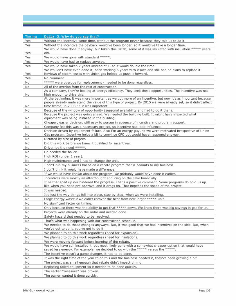
DNV GL – www.dnvgl.com Page C-3
Timing Dat1a_O. Why do you say that? Yes Without the incentive same time, without the program never because they told us to do it. Yes Without the incentive the payback would've been longer, so it would've take a longer time.
Yes We would have done it anyway, but taken thru 2020; some of it was insulated with insulation ***** years old.
Yes We would have gone with standard *****. Yes We would have had to replace anyway. Yes We would have taken 2 years instead of 1, so it would double the time.
Yes We wouldn't have even done it; been working 5 years with issues and still had no plans to replace it. Reviews of steam losses with Union gas helped us push it forward.
Yes No comment. No ***** were overdue for replacement - needed to be done regardless. No All of the overlap from the rest of construction.
No As a company, they're looking at energy efficiency. They seek these opportunities. The incentive was not high enough to drive this.
No
At the beginning, it was more important as we got more of an incentive, but now it's as important because people already understand the value of this type of project. By 2015 we were already set, so it didn't affect time frame; in 2008-11 it was important.
No Because of the window of opportunity (seasonal availability and had to do it then).
No Because the project was going ahead. We needed the building built. It might have impacted what equipment was being installed in the building.
No Cheaper, easier decision, still easy to pursue in absence of incentive and program support. No Company felt this was a necessary project, so incentive had little influence.
No Decision driven by equipment failure. Also I'm an energy guy, so we were motivated irrespective of Union Gas program. Incentive helps a bit to convince CFO but would have happened anyway.
No Dictated by size of project. No Did this work before we knew it qualified for incentives. No Driven by the need *****. No He needed the boiler. No High ROI (under 1 year). No High maintenance and I had to change the unit. No I don't run my business based on a rebate program that is peanuts to my business. No I don't think it would have made a difference. No If we would have known about the program, we probably would have done it earlier. No Incentives were mostly an afterthought and icing on the cake financially.
No It neither sped up nor hindered the progress. That's a positive comment. Some programs do hold us up like when you need pre-approval and it drags on. That impedes the speed of the project.
No It was needed. No It's just the way things fell into place, step by step, when we were installing. No Large energy waste if we didn't recover the heat from new larger ***** unit. No No significant factor on timing. No Only because there was the ability to get that ***** down. We knew there was big savings in gas for us. No Projects were already on the radar and needed done. No Safety hazard that needed to be resolved. No That's what was happening with our construction schedule.
No We needed to do those changes anyways. But, it was good that we had incentives on the side. But, when you've got to do it, you've got to do it.
No We planned to do this work regardless (need for expansion). No We planned to do this work regardless (need for insulation). No We were moving forward before learning of the rebate.
No We would have still installed it, but most likely gone with a somewhat cheaper option that would have saved less energy. For example, we decided to go with the ***** versus the *****.
No The incentive wasn't a game changer, it had to be done. No It was the right time of the year to do this and the business needed it, they've been growing a bit. No The project was small enough that rebate didn't impact timing. No Replacing failed equipment so it needed to be done quickly. No The earlier *measure* was broken. No The owner wanted it done quickly.

DNV GL – www.dnvgl.com Page C-4
Timing Dat1a_O. Why do you say that? No The project had its own merits, so if it was to move forward it probably wouldn’t affect timing. No We can only shutdown the plant during 2 specific times a year. No We had to address the leaks immediately; ***** so they're just wasting money if they left it leaking. No We needed to do this during the summer, a very short window.
No
We were at a point between ***** and the manpower was available to do these projects; already had the budget approved to address the equipment failure because they had been thinking of doing this for some time.
No This was an installation that helped the plant, *****, so it would've happened regardless. No Very attractive on own merits.
No Very likely, the time frame the same; would have done the project anyway; it wasn't - we get a rebate if we upgrade, but we need to upgrade, and hey- we can get a rebate.
No Very likely; same timing. No You need the program to prompt us to think about EE; we have an enormous utility bill. No No comment.

DNV GL – www.dnvgl.com Page C-5
Table 8-10: Efficiency Verbatim Responses for Union Custom C&I programs
Efficiency Dat2a_O. Why do you say that? Yes ***** would have dropped out. ***** may have been harder to justify. Yes Cost reasons. Yes I would have put up the same amount of *measure*, but would have chosen a less efficient product. Yes If there were not incentives, than we likely would have not been able to afford the more efficient options. Yes We had a less efficient design in place. Yes Standard efficiency for the industry that would still support our overall budget.
Yes The program recommended the highest R-value insulation available and rebates are tied to energy savings so greater efficiency leads to a higher rebate.
Yes We didn't know of the insulation opportunity and savings. Yes We wouldn't have had the knowledge about available higher efficiency options. Yes It could have easily affected the technology. We were *****, so may have gone for *****. Yes We just would have went with a cheaper, less efficient version, like we did years ago. Yes Possibly less but just as likely that we would have done nothing at all. Yes The program incentives allowed us to install more measures, greater efficiency. Yes The rebates allow us to purchase better equipment. Yes We would do ***** just to code. Yes Would have been a less efficient *measure*; the old *measure* was 40 years old. No Because I don't think we could have gone any higher with the efficiency. It's pretty efficient. No After analyzing different options, it seemed like the best option for our operation. No We would not have been able to do *****, but we checked them every couple of years. No Considered going with more efficient option, but savings did not appear to be worth the extra money.
No Decision driven by equipment failure. Also I'm an energy guy, so we were motivated irrespective of Union Gas program. Incentive helps a bit to convince CFO but would have happened anyway.
No I would have kept fixing the leaks for the next 18 months then would have to replace it. No High ROI (under 1 year). No I'm looking at the long term on my bill.
No If we are doing the work, we try to replace with best technology available because we've found it often saves us money in the long run and is better ***** (i.e. ***** is clearer and provides *****).
No Incentives were mostly an afterthought and icing on the cake.
No It all comes back to I need to do what I think I need to do to give me the best ROI. If I rely on some government program then we are all in trouble.
No It is the highest. If I decided to go with doing the insulation of the pipe it would have been the same efficiency.
No It was either install it or not. We wouldn't have considered different efficiencies. No It's a guess. It's possible.
No The program did not affect our planning or decisions whatsoever. They were driven by ***** requirements.
No There's not that many choices. No We decided that's what we wanted to do, and they ok'ed it. No We liked what we did, because we saw it at other *****. No We had a set ***** in mind.
No We try to get the most energy efficient options available anyways - if incentive is only 1% of project cost we are going with the same equipment regardless.
No We were going for ***** anyways. The incentive just helped us along. No We would have gotten the same boiler. No You don't know what you don't know. No The efficiency of ***** was part of the engineering design so they wouldn't have changed it. No It's based on the programming, so nothing different. No The payback would've worked out without rebates. No Same efficiency - we have standards that we have to follow. No Same efficiency as it was the best available at that time. No We needed the efficiency that we installed. No We prioritize energy savings.
No We would've gone with the same ***** from the same manufacturer - they've been buying from the same manufacturer for years.

DNV GL – www.dnvgl.com Page C-6
Efficiency Dat2a_O. Why do you say that?
No The vendor ***** recommends an insulation value, after a certain amount adding more insulation doesn't get more savings.
No We would have still picked the most efficient option.

DNV GL – www.dnvgl.com Page C-7
Table 8-11: Quantity Verbatim Responses for Union Custom C&I programs
Quantity Dat3a_O. Why do you say that? Yes Because without the incentive other projects would have become a higher priority. Yes We didn't know of the opportunity and savings. Yes We had another plan in place.
Yes If a steam trap was on the border of needing to be replaced, we may have not completed it without the incentive.
Yes It was such a minor project. Yes It would have been none. Yes We may have done less of the dock seals without the incentives. Yes We may have not replaced all the steam traps at the same time.
Yes We only had a few large leaks and lots of small leaks. We would have only fixed large leaks without incentives.
Yes We were not aware of the steam traps. Yes We may not have done as much testing as we did. But, it would have been close. Yes We needed to do it with utility incentive support or not at all. Yes We wouldn't have *****. With the additional savings. It led to the next project *****. Yes It would have been spread over numerous years. Yes We would not have identified the opportunity without help from Union Gas. Yes Because the project is not scalable. Yes It comes down to spending (the incentives). Yes We definitely would not have done everything we did without the rebates. Yes If it was a proactive replacement, maybe half. Yes The original design was no insulation. Yes Out of the *****, we would have done half. Yes Possibly less, but just as likely that we would have done nothing at all. Yes The rebates allow us to do more. Yes The rebates allowed us to install more measures. Yes The incentive improved the payback and allowed us to replace more valves. Yes There were areas with no doors and garage doors that would have been just left open. Yes There would have been nothing.
Yes We wouldn't have installed energy saving *****; there was a lot that went into the construction of the ***** so hard to say what wouldn't have been done.
Yes We would have done 20% less; incentive helps us get more $ for this year. Yes We would have done 25% of what we did.
Yes We would have done fewer building. We do 2 or 3 per year, so we would have done half. Maybe 1 to code and 1 with insulation.
Yes We would have had no ***** without the program; *****.
Yes We would have only done 25% of what we did; would not have targeted the most important ones; *****, just the ones we could visually locate, the others no.
Yes No comment. No ***** had enough justification on their own. Auxiliary equipment would have changed. No *****, same scale. No The amount of work was need based. No Cheaper, easier decision, still easy to pursue in absence of incentive and program support. No The current condition was a safety hazard. We needed to complete this amount to fix it.
No The decision was driven by equipment failure. Also, I'm an energy guy, so we were motivated irrespective of the Union Gas program. Incentive helps a bit to convince CFO but would have happened anyway.
No We did this work before we knew it qualified for incentives. No Didn't present management with smaller options.
No He would have kept going through the plant piecemeal, eventually getting to the whole thing. This is accounted for in timing.
No High ROI (under 1 year). No I don't rely on rebates to make these decisions. I base the decision on the return on investment. No I would use the source I used to calculate what I needed and install it. No If we did the work, we would have done it the same way. No The incentive doesn't make any difference.

DNV GL – www.dnvgl.com Page C-8
Quantity Dat3a_O. Why do you say that? No The incentives were mostly an afterthought and icing on the cake. No It was a ***** replacement. No It would be very difficult to do anything else. It's all or nothing. You can't do part. No It's a very large building. We had to install the proper equipment in it. No It's just a matter of the size of the *****. There's nothing that I could change. No Just based on this project requirements. There was only one way to do it. There weren't options. No We knew what we wanted. No NA for this project, set amount required for this application regardless No No difference. No Same - Energy savings were large enough to make it worth it, even without incentives. No Scope of projects already determined years prior. No The program did not influence our decisions. No The size of the ***** was decided based on the needs of the process. No The incentive did not affect the amount of equipment that would have been installed. No There is a certain amount needed *****. That can't change. No We had a specific size that we needed. The new one has more throughput. No We had an engineering study completed in order to identify exactly the size of the unit we needed. No To leave some pipe uninsulated would not have made sense. No We didn't want to leave any pipe exposed. No We just replaced what needed to be replaced. No We needed a certain size *****. No We needed to conduct this amount of work, regardless of the incentives. No We upgrade a whole suite of controls; so we needed to do all for it to function properly. No We were moving forward before learning of the rebate.
No We would have done it. We had to do it. The incentive is a great thing. We welcome that. But, the incentive is not going to change the scope of the work.
No It would have been spread over numerous years. No We would have still done the same amount, just may have taken a little longer to get completed.
No The amount of the incentive didn't drive the quantity, it was marginal, so they would've installed the same amount.
No The capacity wouldn't have changed. No It doesn't make sense to do a portion.
No We might've chosen not to do as many steam traps right away, some were just leaking as opposed to failing outright.
No We need the same size to keep up with customer demands for our product. No The quantity was not an issue here; we didn't have an ***** and we wanted one to increase efficiency. No The quantity was not relevant; we needed to replace the fans. No The quantity wasn't the issue here. No We replaced one washer. No It was required. No The same amount but we would have done it less frequently. No The same scale.
No The option with the most savings was to go with the ***** smaller *****; incentives made no difference here.
No We have all sorts of other systems that fit with the ***** - heating/cooling, irrigation, etc. - that we had to get the amount of ***** we did.
No We needed the quantity that we went with. No We needed to address all of the leaks with or without the rebate. No We needed to replace the failed insulation, no more no less. No Ultimately the same amount, but it would have taken us much longer to get through the queue. No We would have installed a lower quality. No It wouldn’t really have an effect. No No comment.
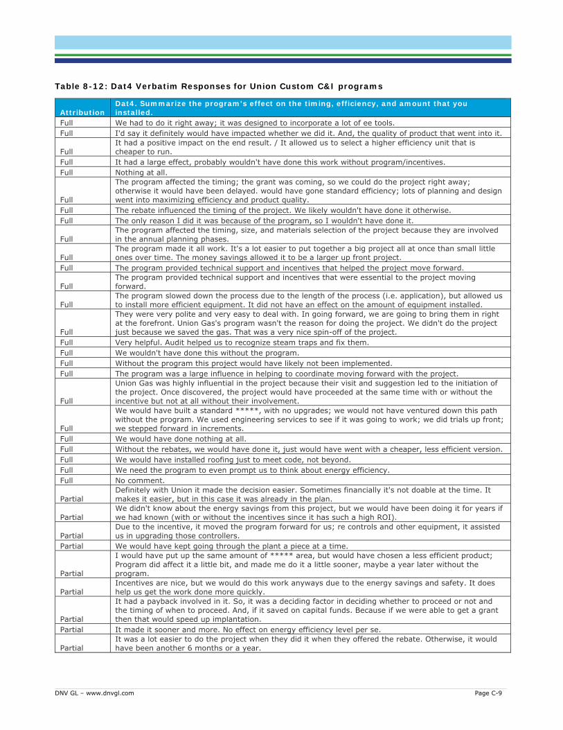
DNV GL – www.dnvgl.com Page C-9
Table 8-12: Dat4 Verbatim Responses for Union Custom C&I programs
Attribution Dat4. Summarize the program's effect on the timing, efficiency, and amount that you installed.
Full We had to do it right away; it was designed to incorporate a lot of ee tools. Full I'd say it definitely would have impacted whether we did it. And, the quality of product that went into it.
Full It had a positive impact on the end result. / It allowed us to select a higher efficiency unit that is cheaper to run.
Full It had a large effect, probably wouldn't have done this work without program/incentives. Full Nothing at all.
Full
The program affected the timing; the grant was coming, so we could do the project right away; otherwise it would have been delayed. would have gone standard efficiency; lots of planning and design went into maximizing efficiency and product quality.
Full The rebate influenced the timing of the project. We likely wouldn't have done it otherwise. Full The only reason I did it was because of the program, so I wouldn't have done it.
Full The program affected the timing, size, and materials selection of the project because they are involved in the annual planning phases.
Full The program made it all work. It's a lot easier to put together a big project all at once than small little ones over time. The money savings allowed it to be a larger up front project.
Full The program provided technical support and incentives that helped the project move forward.
Full The program provided technical support and incentives that were essential to the project moving forward.
Full The program slowed down the process due to the length of the process (i.e. application), but allowed us to install more efficient equipment. It did not have an effect on the amount of equipment installed.
Full
They were very polite and very easy to deal with. In going forward, we are going to bring them in right at the forefront. Union Gas's program wasn't the reason for doing the project. We didn't do the project just because we saved the gas. That was a very nice spin-off of the project.
Full Very helpful. Audit helped us to recognize steam traps and fix them. Full We wouldn't have done this without the program. Full Without the program this project would have likely not been implemented. Full The program was a large influence in helping to coordinate moving forward with the project.
Full
Union Gas was highly influential in the project because their visit and suggestion led to the initiation of the project. Once discovered, the project would have proceeded at the same time with or without the incentive but not at all without their involvement.
Full
We would have built a standard *****, with no upgrades; we would not have ventured down this path without the program. We used engineering services to see if it was going to work; we did trials up front; we stepped forward in increments.
Full We would have done nothing at all. Full Without the rebates, we would have done it, just would have went with a cheaper, less efficient version. Full We would have installed roofing just to meet code, not beyond. Full We need the program to even prompt us to think about energy efficiency. Full No comment.
Partial Definitely with Union it made the decision easier. Sometimes financially it's not doable at the time. It makes it easier, but in this case it was already in the plan.
Partial We didn't know about the energy savings from this project, but we would have been doing it for years if we had known (with or without the incentives since it has such a high ROI).
Partial Due to the incentive, it moved the program forward for us; re controls and other equipment, it assisted us in upgrading those controllers.
Partial We would have kept going through the plant a piece at a time.
Partial
I would have put up the same amount of ***** area, but would have chosen a less efficient product; Program did affect it a little bit, and made me do it a little sooner, maybe a year later without the program.
Partial Incentives are nice, but we would do this work anyways due to the energy savings and safety. It does help us get the work done more quickly.
Partial
It had a payback involved in it. So, it was a deciding factor in deciding whether to proceed or not and the timing of when to proceed. And, if it saved on capital funds. Because if we were able to get a grant then that would speed up implantation.
Partial It made it sooner and more. No effect on energy efficiency level per se.
Partial It was a lot easier to do the project when they did it when they offered the rebate. Otherwise, it would have been another 6 months or a year.

DNV GL – www.dnvgl.com Page C-10
Attribution Dat4. Summarize the program's effect on the timing, efficiency, and amount that you installed.
Partial Medium to large effect, we probably wouldn't have done this work or done less dock seals without program.
Partial
Program had an effect on timing since incentives helped get the project approved quickly by upper management. The program had little effect on efficiency or quantity (for this project - larger projects like a boiler this would likely have a greater effect).
Partial The program impacted the timing of the project but not the quantity or efficiency. Partial The program impacted the timing, efficiency, and quantity.
Partial The program impacted timing, quantity, and efficiency; their projects are entirely dependent on payback.
Partial The program incentives influenced timing, efficiency, and quantity of what was installed. Partial Program is not as important is it used to be in 2008-2011.
Partial The project would have been delayed 12 months and absence of program could have easily affected the technology. We were *****, so we may have gone for plain *****
Partial We would have installed the same amount of square meters (or linear meters) or I just wouldn't have done it at all.
Partial
The program had little effect on the timing. No impact on efficiency for this project, but helped us get more efficient boilers in the past. Incentives helped us do more steam traps than we likely would have been able to do at one time.
Partial The program helped us complete the work sooner/more frequently than otherwise possible and also helped us afford to complete more. Little effect on efficiency.
Partial The program made it all work. It's a lot easier to put together a big project all at once than small little ones over time. The money savings allowed it to be a larger up front project.
Partial They were part of bringing the awareness of that project to us, it helped us with cost justification and calculations and made us aware of the technology.
Partial Union Gas incentives probably helped upper management approve this work, otherwise would have tried to get it approved the next year.
Partial What we did was just identified if we could get an increase in productivity with our ***** then we could take our other ***** off line.
Partial We would have kept repairing the cracked *****, removing sections, etc… and then would have replaced it in 1-2 years.
Partial We would have only fixed large leaks without incentives.
Partial Lower efficiency is not an option, but would not have been able to do it with the level of frequency and intensity.
Partial The program did not influence timing or efficiency, but it did influence the quantity of valves installed.
Partial The program had an influence on the timing of the project and the quantity (for steam traps), but no impact on the efficiency level.
Partial The program impacted the timing, not quantity or efficiency. Partial The program influenced the timing but not the efficiency or the amount. Partial The program prompted us to think about it; maybe would have done half over several years.
Partial The same amount but we would have done it less frequently; with the program we were doing it annually, without the program, we would have done it every 2-3 years instead.
Partial The same time, same size/scale, some components such as ***** and ***** would have dropped out. Partial The incentives were a nice bonus; had no impact on timing, quantity, or efficiency.
Partial The program's largest effect was the assistance in assessing the situation. As far as the rebate program goes, it made it easier to convince the project going forward. Incentive wise it’s a moderate effect.
Partial The Union incentive had a significant effect on size and effectiveness. Without the incentive, it may have proceeded but it would've been harder to justify and smaller in scope.
Partial We would have done half as many *****
Partial We would have done it anyway, but would have done less than half of what we did and it would have taken through 2020; audits helped identify what we needed.
Partial We would have only done 25% of the quantity, only the ones that we could see.
None We could have done it later, but it would have been awkward, looked bad, and potentially damaged the building.
None Essentially, Union makes us aware that the incentive programs are available. They haven't really pushed them in any one direction WRT any specific projects.
None
Everything was in line and turned out very well for us and for Union Gas. Because I had to change the unit, I would do it anyway. Since I had the incentive it was faster for us to go ahead and purchase the unit.
None Everything went smooth. I am thankful for the incentive. There was nothing else we could have done to better the efficiency.

DNV GL – www.dnvgl.com Page C-11
Attribution Dat4. Summarize the program's effect on the timing, efficiency, and amount that you installed.
None Had to do it. Original controls were 11 years old and had reached the end of the equipment life. Were wasting a lot of energy. No effect by program on timing, efficiency, size/scope.
None
I think it was a bonus for the overall project that this incentive was available. It probably influenced the decisions on some of the smaller, gas-fired equipment that we use in the building. It might have contributed to *****.
None Incentives didn't have large impact. Main goal was to reduce heat output. ROI was high enough that we would have done anyways.
None Incentives were nice but didn't have a huge impact since we realized the potential savings from this project.
None It made no difference.
None It would have been a very similar project. But, the incentive helps our decision to go forward and install the components. The timing wouldn't have changed.
None It's great. It didn't effect the timing, efficiency, or amount. None Made it easier to make the case to my CFO but would have happened anyway. None No effect on timing, efficiency, or quantity, since we did this work before learning about incentives. None No effect. None No influence on timing, quantity, or efficiency. None Not much influence. None Nothing in particular. None The program had no impact on timing, efficiency, or quantity. None Safety was the main driver, not the program, although the incentives were appreciated.
None The fact that there's an incentive program provides incentives for doing the project, but it's not the major factor. It helps push this project along.
None The program didn't really effect the timing, efficiency, or amount, but incentives did help.
None
The program had little effect on the timing, efficiency, and amount of work conducted for this project since it was all need based. Other projects they have influence quantity though (i.e. when installing insulation).
None The project was designed. Went on time. We got good results from the project. And we are thankful that we got the incentive from Union Gas for the project.
None The timing was good because everything got completed on time. We didn't know the savings until about 7 months later, when we hit winter. The incentive was a great help.
None There was no effect.
None
There was some effect. There are a few things we might not have done, or the utility support sped the decision. E.g. the ***** and the *****. Would have likely done anyway but taken longer to analyze and decide.
None Utility helped define the minimum efficiency for project and helped improve ROI to get easy approvals from corporate
None We were moving forward before learning of the rebate.
None While the incentives were appreciated, they were not large enough to have much effect on what we installed (timing, efficiency, or amount).
None While we appreciated the incentive, we would have installed the energy curtain anyways to save on natural gas so the program didn't really influence our decision.
None Incentives were a bonus that fit in with their maintenance schedule; program had no influence on timing, quantity, or efficiency
None No impact on the timing and efficiency. The incentives were a nice bonus; always looking for way to get energy savings.
None No impact on timing, quantity, or efficiency. None No program attribution. The program did not impact timing, quantity or efficiency. None The program didn't have an influence on anything. None The program had no influence on timing, quantity, or efficiency. None The program impacted efficiency of equipment; no impact on timing or quantity.
None We would have done the same exact thing that we did. You could get a less efficient deck design but we wouldn’t have picked that.
None
We would have done exactly what we did; the rebate is a bonus on the end; we're making decision based on best payback and most EE; if there’s a rebate, great. If not, we wouldn't do something less efficient because it doesn’t make business sense.
None No comment.

DNV GL – www.dnvgl.com Page C-12
Union Large Volume
This section presents the Union Large Volume self-reported responses from the timing, efficiency, and quantity attribution battery where customers were asked “Why do you say that?”. These responses along with whether a response received some timing, efficiency, or quantity credit are presented inTable 8-13, Table 8-14, and Table 8-15.
A “yes” in the timing, efficiency, or quantity column indicates partial or full attribution for that source based on the scored questions (not the responses here). A “no” indicates no attribution for that source. For example in the first table a “yes” in the timing column indicates that the respondent answered the question DAT1a and DAT1b with responses that credited the program with accelerating the project. A “no” in the timing column indicates that the respondend did not credit the program with accelerating the project. A “no” for timing does not preclude the same respondant indicating the program affected the efficiency or quantity/size of the same project.
Additionally, following the specific timing, efficiency and quantity questions, customers were asked to summarize the program’s effect on the timing, efficiency and amount of the project installed (Dat4). These responses are presented in Table 8-16 with the scored level of attribution: full, partial, or none.
None of the responses provided below were used in the direct scoring of surveys. For respondent confidentiality these responses are isolated from other responses from the interview and do not reflect the full story the respondent conveyed. The responses are provided here to provide insight into how customers describe their decision making on the project relative to the program. See APPENDIX J and APPENDIX K for details on how attribution was scored.

DNV GL – www.dnvgl.com Page C-13
Table 8-13: Timing Verbatim Responses for Union Large Volume
Timing Dat1a_O. Why do you say that? Yes By being aware of everything it helped to speed things up. Yes Do a yearly steam trap analysis and would have discovered the failed traps then. Yes I think because the effective cost of the work was less with the incentive from Union Gas. Yes It helped to move it ahead faster, with the funding. Yes It was creating a *****, one was very fouled, so it had to be done regardless, the 2nd was borderline, and
would have been cleaned the next year if it hadn't been last year. Yes Survey by Union Gas identified the issues, but this would've happened eventually anyway. Yes It was a good project & made sense to do at some point in time. ***** would have given it more priority. Yes No comment. No Already identified and approved as part of infrastructure maintenance - incentives were a bonus. No Company has recognized the need for this due to potential energy savings/ ROI. No Decision driven by needs at the site, not incentives. No Installation was staggered as it was. They chipped away at it. Had to stagger anyway due to their production
schedule and constraints. No It would have had no impact. We would have implemented the project with or without the program rebate. No It's a larger project. So, the relative effect of the rebate is not as great. No Needed to be replaced. Incentives were too small to have an effect (incentive less than 1% of project cost). No Only the one window of time for spring maintenance projects. No The incentive is appreciated. But, I can't delay such a large maintenance item. No The project was feasible on its own merits and management expected them to implement it. No These issues are important to the continuing operation of the plant and they are addressed as quickly as
they can be. No Timing determined by turnaround cycle. No We planned to do it regardless of the program. No Because of equipment age (turnaround). incentive helpful to engineering group, but small compared to
whole project. Incentive less than 1% of project cost. No Because of equipment age. incentive helpful to engineering group, but small compared to whole project.
Incentive less than 5% of project cost. No Because won't have another ***** until ****, so take advantage of that opportunity or lose out on it. No It needed to be replaced. No The program had no influence on these projects. These were maintenance issues that needed to be done
regardless and met payback requirements without incentives. No Repairs, so they had to happen. No It was part of a larger project. No We had to do the one as it was failing, the 2nd would have been done in the next couple of years if we didn't
do it at this time, it would have failed in 2-3 years. No No comment.

DNV GL – www.dnvgl.com Page C-14
Table 8-14: Efficiency Verbatim Responses for Union Large Volume
Efficiency Dat2a_O. Why do you say that?
Yes Because they made us aware of the potential energy savings of going with what we did. And, they actively lobbied us for it.
Yes No comment.
No As a ***** manufacturer, we understand going with higher efficiency product will save us money in the long run. Plus already had scope approved by president/director.
No Energy savings justify on its own. No Engineering standards. No More efficient units like the one we got would pay for themselves, even without the incentive.
No It needed to be replaced. Incentives were too small to have an effect in this case (for other projects incentives have helped us afford more efficient equipment, but depends on ROI).
No We picked this ***** because it was the best operational decision. It's just good business practice to install the highest efficiency that we could install.
No We would have selected same product. No We needed the amount of insulation and the type that we installed.
No We had to do the one, the 2nd would have been done in the next couple of years if we didn't do it at this time, it would have failed in 2-3 years.
No Would have gone ahead with same ***** project anyway. No No comment.
Table 8-15: Quantity Verbatim Responses for Union Large Volume
Quantity Dat3a_O. Why do you say that? Yes We would have gone with an option that did not increase the efficiency of the system. Yes One ***** needed to be replaced due to corrosion, but the rebate allowed us to do the 2nd one at the
same time. Yes Would be influenced. Yes No comment. No *Measure* needed to be replaced anyway. Maintenance ***** needed to be done anyway, and was
already scheduled. No Already identified and approved as part of infrastructure maintenance - incentives were a bonus. No Certain constraints in terms of safety standards. No Decision driven by needs at the site, not incentives. No Maintenance standards. No NA - only 1 was needed. No Needed to be replaced anyway. No Needed to be replaced. Incentives were too small to have an effect (incentives less than 1% of project
cost). No The program is beneficial; it puts money back into their pocket. Like sprinkles on cake (extra $). No The simplicity of the project. What we were implementing was just standard practice. There was nothing
we would have done that was out of the ordinary. No There wasn't really an option to do only part of it. No It was based on engineering standards, not on program incentives. No We had a pretty good idea of what we were going to do. We spent a lot of time determining the scope of
the work. At the time we are thinking, it is not guaranteed that we will get the rebates. So, it is a bit of an educated guess.
No We had to install the amount we did. The incentive contribution was not material. No We needed the insulation they installed, and we wouldn't have changed this. No We needed to replace ***** failed steam traps anyway, would just have been delayed. No Only one choice. No Repairs are necessary. No Same amount but this would've had to happen over a period of time / piecemeal. No This was what we needed, and we incorporate the program in our planning process. No It was new construction/***** project, one window of opportunity. No We would have been installed anyway on own merits. No No comment.

DNV GL – www.dnvgl.com Page C-15
Table 8-16: Dat4 Verbatim Responses for Union Large Volume
Attribution Dat4. Summarize the program's effect on the timing, efficiency, and amount that you installed.
Full The program provides commitment to the project. Gets it done.
Full
They were instrumental in helping us to identify the potential energy savings, which expanded the project's scope. But, resulted in a long-term cost benefit to our organization. The program was very helpful in convincing the powers that be that the more expensive option was the best one to pursue.
Full Would not have installed absent the program. Would have kept as-is. Full No comment.
Partial Incentives helped motivate staff to get going. The project was done slightly earlier and on a larger scale than it would have been absent the program.
Partial It improved the timing because of the availability of the rebate. The efficiency and the scope would have remained the same. We couldn't have done less work than we did.
Partial Program provides commitment to project. Gets it done. Partial The timing, the program made it happen sooner. So, we gained the savings sooner. Partial Very likely to install same equipment, 36 months later, same efficiency, same quantity. Partial Very likely to install same equipment, would have been delayed 18 months.
Partial
We would have done less and less frequently. We would have likely done it, but 6 months later when we have downtime, on a smaller scale. We would do 75% and not replace ***** until they were closer to end of life because of program education we understand ***** efficiency.
Partial
Its hard to say, would have done half as many 2 years later. We would have wasted more fuel, traps are something we observe; years of patching up equipment. Now it's maintenance annually due to program ed.
Partial One ***** needed to be replaced due to corrosion, but we did the 2nd one at the same time because of the rebate, but it had some RUL.
Partial The program influenced timing and quantity.
Partial The program accelerated the installation by 12 months and caused a larger amount of steam traps (half of those that were incented) to be replaced.
Partial The program accelerated the installation some, and caused a larger amount of pipe insulation to be replaced but the respondent didn't know by how much for either.
Partial
We would have been somewhat likely to do it, because we knew what we were doing. It wasn't a good thing to do, but would have been 6 months later because we didn't know how much fuel we were wasting, but in keeping with same scale/efficiency.
Partial We would have done the same thing; rebate was influential in getting us to do the *****; incentive pushed the 2nd project to this year, instead of the next year; utility rebate makes the payback better.
None As mentioned before, the utility mainly just provided the incentive quote/estimate, but did not have much effect on anything else.
None Honestly, we were set on doing this as an infrastructure improvement and would have done it all the same without the incentives.
None Incentives can help for certain projects, but when they are relatively small they don't impact our timing, efficiency, or amount. Still helps, but doesn't sway us.
None It had no effect. It's a good program that helps people make better business decisions in terms of installing the best, efficient materials and equipment and, therefore, making better business decisions.
None It triggered an awareness that there were many more projects that we could implement. It put us in that frame of thought and helped encourage us.
None It would have affected if and how soon the project got approved. None No effect on timing, efficiency or size/scope of what they installed. Would have done anyway. None No effect. Decision driven by needs at the site, not incentives None No effect. Would have been same timing, efficiency level and size/scope.
None
Program had little effect on the decision to do this work, because it was necessary for the safety/continuing operation of the facility. Also little effect on efficiency and quantity, due to engineering and maintenance standards respectively.
None Project was very likely to be implemented without the Union Gas program, at the same time, efficiency level and size/scope.
None The program had essentially no effect on this work at all (timing, efficiency, or amount). This was work we planned to do regardless.
None The project would have been done at the same time, efficiency level and size absent the program. None Very likely to install same equipment, same time, same efficiency, same quantity.
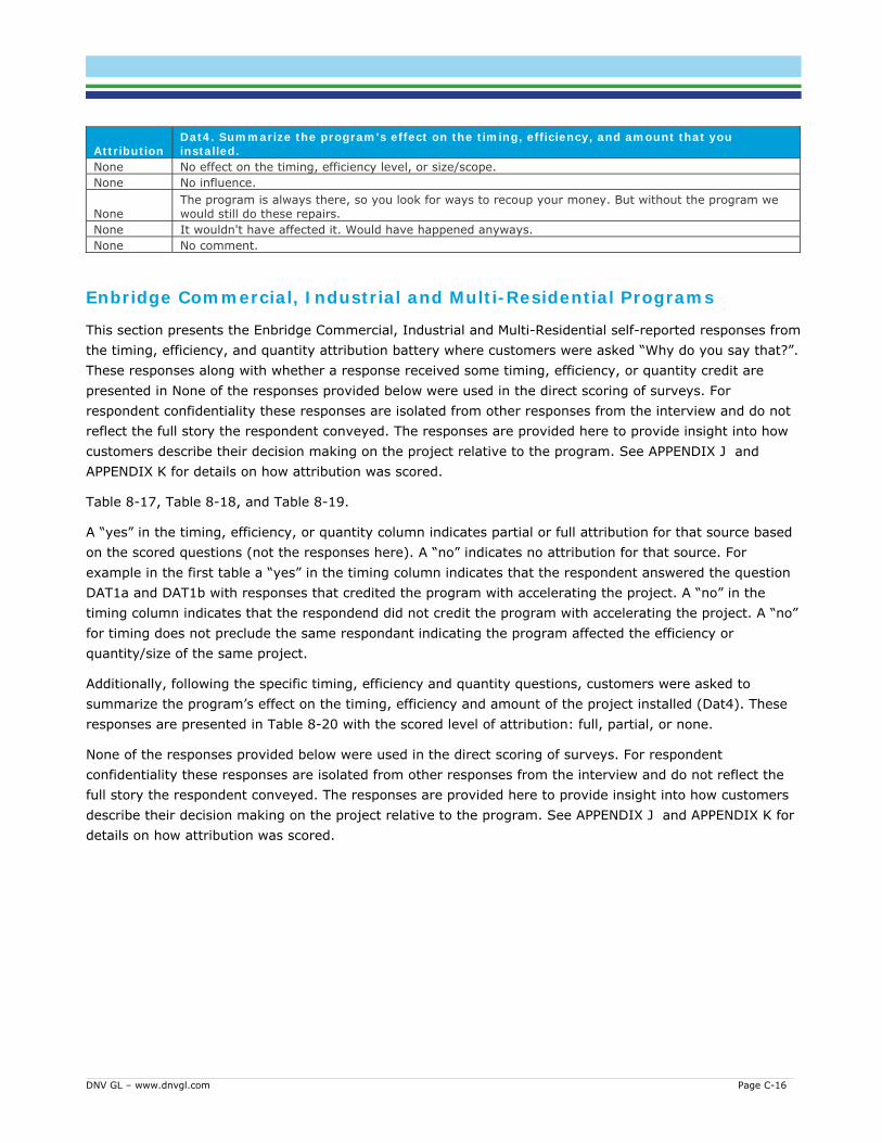
DNV GL – www.dnvgl.com Page C-16
Attribution Dat4. Summarize the program's effect on the timing, efficiency, and amount that you installed.
None No effect on the timing, efficiency level, or size/scope. None No influence.
None The program is always there, so you look for ways to recoup your money. But without the program we would still do these repairs.
None It wouldn't have affected it. Would have happened anyways. None No comment.
Enbridge Commercial, Industrial and Multi-Residential Programs
This section presents the Enbridge Commercial, Industrial and Multi-Residential self-reported responses from the timing, efficiency, and quantity attribution battery where customers were asked “Why do you say that?”. These responses along with whether a response received some timing, efficiency, or quantity credit are presented in None of the responses provided below were used in the direct scoring of surveys. For respondent confidentiality these responses are isolated from other responses from the interview and do not reflect the full story the respondent conveyed. The responses are provided here to provide insight into how customers describe their decision making on the project relative to the program. See APPENDIX J and APPENDIX K for details on how attribution was scored.
Table 8-17, Table 8-18, and Table 8-19.
A “yes” in the timing, efficiency, or quantity column indicates partial or full attribution for that source based on the scored questions (not the responses here). A “no” indicates no attribution for that source. For example in the first table a “yes” in the timing column indicates that the respondent answered the question DAT1a and DAT1b with responses that credited the program with accelerating the project. A “no” in the timing column indicates that the respondend did not credit the program with accelerating the project. A “no” for timing does not preclude the same respondant indicating the program affected the efficiency or quantity/size of the same project.
Additionally, following the specific timing, efficiency and quantity questions, customers were asked to summarize the program’s effect on the timing, efficiency and amount of the project installed (Dat4). These responses are presented in Table 8-20 with the scored level of attribution: full, partial, or none.
None of the responses provided below were used in the direct scoring of surveys. For respondent confidentiality these responses are isolated from other responses from the interview and do not reflect the full story the respondent conveyed. The responses are provided here to provide insight into how customers describe their decision making on the project relative to the program. See APPENDIX J and APPENDIX K for details on how attribution was scored.

DNV GL – www.dnvgl.com Page C-17
Table 8-17: Timing Verbatim Responses for Enbridge Custom C&I programs
Timing Dat1a_O. Why do you say that?
Yes
*****: delayed a year w/o rebate – it still would have gone, but maybe 60%chance it was done that year/40% chance next year; *****: would have to do something at some point...maybe delayed, it would not go to ruin but it could be neglected longer.
Yes Because having a stronger business case will give us better payback and the project will become more viable and more likely to get approved and funded.
Yes I don't know for this specific project - but incentives frequently expedite getting projects approved. Yes It is easy to justify in the project budget. Yes Enbridge's program created the business case for us. Yes Eventually we would have gotten to it, such a large saver. Yes I would have added ***** instead of doing the *****. But, I would still have had to add *****. Yes The incentive matters. Yes Incentives are included in our budget forecasting. Yes Incentives helped the director approve the project. We may have been delayed it without incentives.
Yes Incentives made it easy to get approved (brought it within 2.5 yr ROI). May have got pushed back without incentives because more convincing would have been necessary.
Yes It would have been much later if not never. Yes It wouldn't have had the payback. It would have been beyond our guideline.
Yes It's the business case. The incentives shore it up. Without that funding, it throws off the numbers, we need to secure more internal funding.
Yes Just because of the ROI. The incentives made it happen. They put it over the edge. Yes Likely would not have done it without incentives due to maintenance costs/hassle to keep them clean. Yes Money. Yes Our location is closing, so it would never have happened.
Yes Probably a little bit later because general awareness of incentive was lower. Enbridge turned them on to other incentives.
Yes The *process* for ***** relatively expensive for the expected ROI. As a result, upper management would not likely see value without the incentive.
Yes The incentive helps focus people's attention in terms of getting the job done. They help us in highlighting these measures as opportunities.
Yes The incentive raised the profile of the project in comparison to its size. Yes The math showed them the savings to get the ***** installed. Enbridge helped with the math.
Yes The program is not just an incentive thing. The thing for me that is equally important is the parternship in terms of identifying and vetting different project ideas.
Yes They incentivized the steam trap audit as well. Yes They now do this every year. This is an odd question.
Yes They were still considering energy savings and wanted to be proactive. They like the incentive. If there weren't an incentive, they would do another project first.
Yes They would do it every three years, but not every year. Yes They would have done them piecemeal over time.
Yes Upper management would have likely not approved a project like this that is not viewed as an immediate priority.
Yes We had to do it. But, the incentive helped us to do it faster. Yes We wouldn't have been able to justify the payback without the incentive. Yes Without incentives the project would not have been approved/ we wouldn't have done the project. Yes It would have been pushed off. Yes We would have had to wait until next summer to get it in the budget. Yes We would have likely still replaced one at the same time, and then the second one at a later date. Yes We would have replaced on equipment burnout.
Yes We would have taken longer to be aware of the savings opportunity. Plus the incentive was relatively large and a significant motivator.
Yes We would have taken longer to get appropriate resources and funding in place. Yes We wouldn't have had technical or financial support.
Yes It's not a small project *****, so it takes time, lots of operations, keep the plant running all the time, started 2011, ended 2015, rebate accelerated the project by one year.
Yes The rebate helped the payback work out. Yes The rebate reduced payback so they could install measures sooner.

DNV GL – www.dnvgl.com Page C-18
Timing Dat1a_O. Why do you say that? Yes The rebate helped the payback allowing them to do the project sooner. Yes Tough to say; they have tight ROI metrics. Yes It would have taken longer to convince them to do.
Yes It would've been replaced eventually, but they don't typically become aware until an audit or something breaks down.
Yes No comment. No ***** replacement was due No ***** was a regular maintenance item. ***** were something they wanted for growing reasons. No Aiming to meet internal efficiency goals.
No Because of our business model. We work in *****. We only have a short window to ***** because of the weather.
No The incentive is a very small percentage from the project cost. No The unit was old and needed to be replaced. No Because we were going to change the boilers whether there was any incentive or not. No The Enbridge program was not a factor. No End of useful life, savings with gas when replaced.
No
The equipment had failed and we needed a replacement. The decision was driven largely by the larger Toronto Hydro incentive. The small Enbridge incentive relative to the large total project cost wasn't a big motivator.
No The equipment needed replacement.
No
I think that moment when you are trying to decide, knowing that there is some extra funding pushes you to do it. Enbridge's involvement had more to do with whether we would do it or not do it than the with timing of doing it.
No I would still implement it. It's more of an operational savings. We are going to get savings with the Enbridge program or not.
No The idea came from us and our president.
No It's the business case. The incentives shore it up. Without that funding, it throws off the numbers, we need to secure more internal funding.
No Leaks needed to be fixed, it's very expensive for the company to continue operating "as is/was".
No Motive was for improved plant conditions, only found out about incentives after we were set on doing project.
No It needed doing. No We needed to get this work done for energy efficiency purposes. No Once we discovered the need we like to move on them, given the circumstances. No Refused. No Similar time because we have a 5 year plan on spending on this type of project. No Simply because the payback was justifiable. No That was the time when we were able to identify it. The program being in place just helped us move along.
No The Hydro Incentive was bigger. The Enbridge incentive was great. It made the ROI that much better. It was a bonus. But, it was the Hydro one that made the case for this project.
No The boilers were falling apart. Try to submit early in the year when people aren't busy, timing for tender is very important.
No The drivers for the projects didn't have much overlap with the Enbridge reps; they provide only a very small portion of total funding; they're not at the table.
No The incentive makes it a real no brainer, but it's a decent business case without it. The decision is weather driven, so we do it every year but could do it every other year without the incentives.
No They needed to be done. No They were a pile of rust. No This one would probably have happened at this time, though in a smaller way. No This was a construction project which was scheduled for other reasons. No Timing was coordinated by the energy office. No We had planned to do this replacement per our schedule. No We had to change the equipment. Enbridge just helped us with installing energy efficient equipment.
No We had to have the ***** shut down at the time we made the installation. Those shutdowns aren't very frequent. We had a scheduled outage. And, the equipment was here. So, that's when we installed it.
No We had to replace the *****. No The maintenance had to be done. No It didn’t affect timing.

DNV GL – www.dnvgl.com Page C-19
Timing Dat1a_O. Why do you say that? No We had to address safety issues. No It had to be done during shutdown. No it was a quick, small project; no capital investment involved. No leverage ***** No One of the boilers was failing critically. No The project was under the 1-year ROI, but the rebate made the ROI lower.
No The rebates were not a factor in the timing. We were going to do these projects with or without the incentives.
No The rebates were not a factor in the timing; We were going to do this project with or without the incentives. No The system was broken. We had to replace. No We planned these projects well before they knew the rebates existed. No To improve process efficiency. No No comment.

DNV GL – www.dnvgl.com Page C-20
Table 8-18: Efficiency Verbatim Responses for Enbridge Custom C&I programs
Efficiency Dat2a_O. Why do you say that? Yes Incentive changed the cost/benefit calculation.
Yes Incentives helped get a more efficient unit approved. *****, so may have gone with unit of a similar efficiency - hard to say.
Yes Might have gone less efficient. Hard to know. Yes The program incentive helps improve PP. Yes The incentive helps to install a higher efficiency equipment. Yes We would have gone with a lower efficiency. Yes We would have replaced like for like without the rebates.
Yes I don’t know for this specific project, but possibly less efficient equipment if that was the only way they could get it approved.
Yes We would have installed more than standard but not quite high-efficiency. Yes The rebates allowed them to pursue more efficient equipment. No Again, the decision wasn't driven by the Enbridge incentive. No Consultant recommendation. No Enbridge is just a small player in the financing and decision making for these projects. No Enbridge's involvement is mainly to do with verifying what they did. No influence on efficiency. No Energy savings is important to us No If we are going to do it, we'll do it right. The goal was to increase efficiency. No If we were to do the *****, we would have done it in the most efficient way possible. No We installed the equipment suggested by our vendor. Incentives did not influence the choice.
No Just energy savings after the fact. I am very conscious of the environmental energy cost, its just second nature to my training, how are we going to be better.
No ***** driven No The ***** requirements were the driver for getting the *****. No The big ***** was supposed to be more efficient. No The equipment we selected meets our own internal high standard and yields payback over time. No We don't care about the rebates. No We wanted to install the best and latest technology. No We bought a used unit that became available. We did not custom buy it. No We needed a ***** that would be faster because of the increased usage. No We put the best possible solution at the time in place.
No We try to install the most EE boiler money can buy, we know that in the long run you save on operating cost.
No We try to update our equipment with like for like, efficient alternatives regardless (this is why we consult energy experts first).
No We wanted to use the equipment we used. No Without incentives the project would not have been approved/ we wouldn't have done the project. No We would have replaced it with the same efficiency levels. No It wouldn't make sense to spend the money without getting the savings. No Just ***** installation and some ***** to control it. No There was only one option other than *****, which is ***** and that's what we did.
No We had a good idea of what we wanted based on previous experience. We wanted to save money by increasing energy efficiency.
No We knew what we needed. No No comment.

DNV GL – www.dnvgl.com Page C-21
Table 8-19: Quantity Verbatim Responses for Enbridge Custom C&I programs
Quantity Dat3a_O. Why do you say that? Yes Because the program helps offset the difference in the price cost. Yes Because we would have less incentive. So, the payback would have been less. So, there would have been
less money to be spent. Yes Enbridge made us aware of the type of equipment that was available. Yes Enbridge's incentives and assistance in annual planning is critical for the implementation of most non-
mission critical projects. Yes If there is no incentive, then we might go for less. Yes If you can get incentives to do something, then you will do a better job just because of the cost reduction. Yes It all come backs to it being one system. You are either installing it or not. Yes May have only installed 1 or 2 *****. Yes Not immediate priority due to lower ROI. Yes Only one *action* was necessary to recover heat. Yes Same reason, budget would have had a smaller scope. We may not have adjusted the dampers. Yes The cost savings with the program. Yes The incentive made it cost effective enough that we could get approval from our finance team. Yes They might do however many steam traps they could afford, which is often not much. Yes They would have done one of the ***** boilers. Yes They would not have done this project otherwise. Yes We needed it. Yes We would have gone with like-for-like replacement of the old system, which was smaller. Yes We wouldn't have been focused on identifying the traps that needed replacing. Yes Without the proper ROI we would have had to come up with some other design or something to get it
approved. But, I don't know what that would be. Yes Without incentives, the project would not have been approved/ we wouldn't have done the project. Yes We would have likely replaced the seal/bumper on one door, then another later on. Yes We would have probably not done any without incentives. Yes We would have still done both since we were focusing on renovating non-critical office area. Yes We wouldn't have been aware of the value and need. Yes We would have just done one *measure* instead of two. Yes No comment. No All units were at the end of the useful life. No Amount was needed for significant improvement. No The audit service provided by the utility was very helpful. But the incentives did not impact the choice. No Basically, we don't get to see incentive money, it goes back to ***** and might be used somewhere else. No Enbridge is just a small player in the financing and decision making for these projects. No Engineer and vendor recommendation. No The equipment needed replacement. No Every site needed a new ***** No The extent would have been the same. No It had to be compatible, but increased efficiency was part of 5 year goal. No I don't think the incentive had any bearing on whether we were going to do this project. No It all come backs to it's one system. You are either installing it or not. No It had merits on it own. It had its own justification, even without Enbridge's rebate. No It was a comprehensive project for all mechanicals by design. No It's because of the financials. No It's just a maintenance thing they had to fix. No It's was the option we needed to save money. No Just have 1 heater. No Leaks needed to be fixed. It would be expensive for the company to not repair. No Likely would have done less, and only completed a few of the ***** one year and more the next. No We might have gone with a smaller system. No We needed to replace them all at once to get a better price from the vendor. No There was no influence on size or quantity of boilers installed. No I'm not certain, but I believe only one needed to be replaced.

DNV GL – www.dnvgl.com Page C-22
Quantity Dat3a_O. Why do you say that? No No influence on sizing. No Not scalable; had to control all ***** fans. No We only need one unit. No We only needed to replace the one. No The project needed to be done together because of co-location of *****. No The quantity was based on ***** advice based on square feet. We would install as many as they advised
since they had most experience with them. Not dependent upon the incentive. No The repair had to be done to address safety concerns. No The ***** was more influential. No The ***** requirements was the driver for getting the EE points. No The equipment was sized based on the amount of *process*. No The equipment we selected to meet our own internal high standard and yields payback over time. No The incentive was just a bonus. We had to do this. No The size we went with fills the need. No They go based on the building size. No They sized it for the building. No They wanted to try it, which is what they did. No They were a system. Replace all at once. No They were sized for the building. No They would do the audit and replacement the same, just less often. No Vendor. No We needed it. No You can't do less because of the type of work we do. You can't do a portion and not do the other portion. No Because the units that were being replaced all work well together hand-in-hand so it was advantageous to
do a whole replacement instead of partial. More practical and cost efficient. No The decision wasn't driven by the Enbridge incentive. No Just a longer period of time. No We needed the size for health and safety. No Not scalable. No The same process, both buildings. No The same size either way. No The same, with controls, you can't say do more/less, you have to do it. No Still gone after at the same time because of internal drivers, good business case. No The failing boilers needed to be replaced. No The project would have been the same without Enbridge support as the old system was broken. No We needed to redo the ductwork system, so nothing would've changed without rebates. No We needed what we got; the rebate had no impact on this. No We were only looking to install one VFD. No It would've gotten replaced but later, as they failed. No No comment.

DNV GL – www.dnvgl.com Page C-23
Table 8-20: Dat4 Verbatim Responses for Enbridge Custom C&I programs
Attribution Dat4. Summarize the program's effect on the timing, efficiency, and amount that you installed.
Full Enbridge's incentives and assistance in annual planning is critical for the implementation of most non-mission critical projects.
Full It helps with the timing. Some of the projects would never happen at all if it wasn't for the analysis. The efficiency is improved as well. The analysis helps determine how to make the project a better option. They help with the overall outcome by providing the technical support and some of the fi.
Full The program had large impact on timing and amount. Very likely this work would have not been approved without incentives.
Full Program had little effect on timing or efficiency for ***** project (because it was a HUGE energy waste and had a very high ROI = needed to be done), but had large impact on ***** - made this project feasible.
Full The funding made the project viable. Without the funding we wouldn't have been able to do it. Full The incentive and the program through Enbridge allowed us to get a program completed that we
probably wouldn't have without their help. They helped us simplify the project and implement it in a timely manner.
Full The incentives had a very large effect. If we didn't have them, the ROI would have been over 3 years and the project would have never been approved.
Full They originated the project, the business case. They helped with the assessment which helped accelerate the process of approval with the incentives and a faster ROI.
Full They provided evidence that this was a good thing to do, and they put their money where their mouth is.
Full We would have installed a standard efficiency boiler otherwise. Full When I give them the number of exhaust fans that I have. And, I give them the ***** units that I have,
they did the calculations to balance the system. / When I learned that there is an incentive then I can spend a little more money than what I planned to. With the incentives, we could install a *****.
Full With the incentives and the individual help from Enbridge it helped us reach the proper ROI and make the project a reality.
Full Without incentives, we would most likely not have done this work, so large effect on timing and amount. Full Without the timing, it would have been delayed indefinitely. Full We would have installed all ***** boilers at the same efficiency. Full No comment. Partial Absent the program and incentive, the controls projects would have been implemented eventually,
about 12 months later. The program had no impact on the efficiency level or size dimension. Partial Big influence. The incentive is a great help to the corp. Without the incentive, they would not move the
project forward that soon. Partial By having the incentive, it does increase our ability to save money sooner rather than later. And, it
increases our ability to get it done sooner. Partial I suspect this work would have taken longer to get approved and we may have had to settle for a less
efficient unit without incentives. Partial Certainly, a relevant bonus to us, we got 5% back, but again, overall, project would have proceeded
regardless Partial Enbridge's incentives and assistance in annual planning is critical for the implementation of most non-
mission critical projects. Partial Hard to say for a lot of these (since hypothetical), but incentives helped get this work approved. Without
incentives, we may have done it later, or only 1 maybe 2 of the economizers at this time. Partial I think Enbridge's program for subsidizing steam trap studies and replacement of faulty traps ensures
that we do it on a regular basis and a higher frequency than we otherwise would. Partial If we didn't have the assistance the project would not have been completed to the extent that it was.
And, it would have been much later that we got the job done. We would have not experienced the improvements in production.
Partial Incentives helped bring down ROI which made it easier to get approved. We would have likely done a less thorough job and later without incentives, since the bottom line is critical here.
Partial It helped us install it a year early. Partial It improved the business case and made the decision process easier. Also, it invites more rigor for
measurement and verification which makes it easier for us. Partial Program incentives helped us afford a more efficient option, but didn't impact timing/quantity since all
units were overdue for replacements. Partial Program incentives helped us complete both ***** at the same time. Otherwise would have done work
in two stages.

DNV GL – www.dnvgl.com Page C-24
Attribution Dat4. Summarize the program's effect on the timing, efficiency, and amount that you installed.
Partial Sped up installation, improved efficiency, and had no effect on quantity for this one site. Partial The Enbridge rep made them aware of the incentive for the VFD measure and got the process started.
The VFDs were installed 24 months before they would have been absent the program. No effect on the efficiency level or size/scope.
Partial The incentive and help with calculations of paybacks were important. Easier to make the business case and sell it to VP level to get funded. It clarifies the driving factors and provides outside proof that it will save money.
Partial The incentive program helps in specifying energy efficient equipment. Also, the coordinator helped in answering questions for optimum energy equipment. Also, to help in reducing the cost of the project.
Partial The incentives helped them to implement the project in 2015. Else they would have replaced it on burnout, perhaps a few years later.
Partial The key was our Enbridge contact making us aware of the incentives. Then our consultant ***** identified the failed traps and the quantitative savings opportunity. We would have done fewer traps and significantly later without the program's role.
Partial The program definitely helped us to create the business case. Without Enbridge's help we would not have looked in depth at the ***** project. They helped during the assessment which helped create the business case for the payback. And, they helped direct us to manufacturers to help replace the equipment. The incentives helped us move forward faster on the process of approval. And, the money helped us to do more. And, giving us the incentives gives us a lot of visibility.
Partial The program has very significant influence on the timing and efficiency of the projects but it promotes the selection of the smaller or easier projects as opposed to larger or more complicated projects.
Partial The program helps in specifying the equipment. So, the program helps in offsetting some costs for us. Partial The program incentives helped us increase the project scope and improve overall ***** efficiency, but
did not have much effect on the timing. Partial The program was the main driver in the maintenance manager initially becoming a steam trap
champion. Partial The timing was okay. We got our incentive as soon as we finished the project. So, it gave us incentive to
finish it quicker rather than later. We are satisfied with it. We are happy with the program. Partial There was a small effect by the program on the timing of installation. The measure would still have been
installed, but about 12 months later. Partial They had key inputs in helping ***** upsize to bigger more efficient equipment. Partial They helped us do the audit every year rather than every three years. Partial They raised the profile of the project as they have done for other projects like boilers. Partial We would have done one boiler to see how it went otherwise. Partial Without the incentive, we would have had to wait until the next year at least. Partial Without the program incentives, we may have not done this work as soon or as thorough. Partial We would have installed them two years later at a lower efficiency level. Partial We would probably have done these piecemeal over time. Partial We would still have gone after the same projects because of internal drivers, good business case. Partial All or nothing, same upfront costs, let’s not waste time doing half and half again; it may have affected
repairs if I didn’t have enough $. Partial It influenced the timing, but that's it. Partial The program had an influence on the timing due to incentive. Partial The program impacted timing and efficiency. Partial The program influenced timing, nothing else. Partial The program only influenced timing. Partial The program rebates influenced the timing, nothing else. Partial The insulation before was deteriorating so we had to put it back; with the rebate we could put in
something more efficient to capture everything; controls would have done the same efficiency/quantity. Partial We would have replaced *measure* with the same *measure* instead of spending $ modifying the
piping to install *measure*, but that would only be good for 2-3 years. None It was nice to have that money, it wasn’t what pushed it to do it. Aged equipment needed replacement. None We were already set on doing this project before we became aware of incentives, so the program did
not have an impact on timing or efficiency. Quantity only based on advice of product specialist. None Audit service provided by the utility was very helpful. But the incentives did not impact the choice, size,
efficiency or timing of the project. None Enbridge did not have influence. Rebates were nice to have but not the driving force.

DNV GL – www.dnvgl.com Page C-25
Attribution Dat4. Summarize the program's effect on the timing, efficiency, and amount that you installed.
None Enbridge didn't have as much impact on this project as the Toronto Hydro incentive. Enbridge's was an additional incentive that we could go for. But, it was just a bonus. We received a larger incentive from Toronto Hydro. Don't get me wrong. We love the Enbridge program. But, the Toronto Hydro incentive was more influential.
None Enbridge incentives were good but did not impact the scope or timing of the project. None Enbridge reps; they're not at the table; we remember there's money there and we always apply for it
because we want to apply it forward; but you’re not even a 5% share; 100% goes back into other projects.
None Enbridge's incentive on the project didn't have much effect on the timing. It was an expensive project. So, the incentive was a smaller portion of the total cost than with other projects. So , it was nice. But, the project was going to go ahead with or without incentives.
None Enbridge's support allowed us to make a decision to move ahead quickly. Their technical support helped us make the decision. And, the financial support also helped expedite the decision.
None I just plan it the year before. I've got a budget. You get a rebate. But, because I have to tell them the year before, I have to tell them about the project. You tell them everything that is going to happen the year before. It makes it easier to do the project because there is an incentive.
None Incentives helped, but we would have done the project the same without it. None Incentives were helpful to get work approved, but we would have done mostly the same since we had it
on radar with our internal 5 year energy savings plan. None It didn't affect the timing. It didn't affect the scope. It stood on its own merits. So, it was a bonus that
we got a rebate check at the end. But, we still would have pursued this anyways. None Makes the decision a no brainer i.e. much easier to do. None Minimal effect on timing, efficiency, and amount installed for this project, since we had planned to
replace this anyways since it was at the end of its expect life. None No effect. None No impact. We know that there's incentive money coming, but if we have to replace, we just go ahead
and do it. None None. None Not a huge effect. None Not much effect, since it needed to happen right away due to failed equipment and since larger *****
Toronto Hydro incentive was the big driver. Still, every piece played a part in overall financing and decision making.
None Program had no influence on timing, quantity, or efficiency. None Program incentives didn't effect timing, efficiency, and amount installed since the leaks needed to be
repaired. None Rebates were nice but didn't make a difference. None Since we knew about the incentives before we started planning, the program might have increased the
efficiency level of what we installed. Not sure, though. In terms of timing and what we did, we were doing the whole thing regardless.
None The Enbridge program was icing on the cake for us. We would still have implemented the program regardless of the Enbridge program. The operational savings and the energy savings had more impact than the incentive and rebate.
None The owners tend to take rebates into account. None The program had no effect on the project, and it would have gone forward at the same time, efficiency
level and size absent the program. None The program had no effect on this project; it had to be done to address safety issues. No effect on
timing, efficiency or size from the program. None The program just really didn't have an effect on whether we would do it or not. The timing was good and
it made it get approved. None There was no impact on this boiler project. It was just another thing to go and get because it was
available. The impact on Project 1 was more. None These projects were well on their way before they became aware of the rebates. None This project had to be done at the time that it was (during shutdown) and the program had no impact
on the efficiency level or size dimension. The company would have installed the same technology regardless.
None This project we would have done otherwise. None To get the incentive, audits and repairs have to follow a specified methodology, so it's high as well. The
program's existence tightens up our process.

DNV GL – www.dnvgl.com Page C-26
Attribution Dat4. Summarize the program's effect on the timing, efficiency, and amount that you installed.
None When we planned to replace the door we knew we had to replace the door. Our general manager said to contact Enbridge to see if there is an incentive that we could get. They came over and looked at our plan. They told us there is an incentive and this is what it is going to be. The Enbridge incentive gave us a boost to do it. It went through faster.
None We would have done these anyhow. None Installation had to happen, rebate was a nice bonus. None No influence on timing, quantity, or efficiency. None No program influence on timing, quantity, or efficiency. None The program did not have any influence on the timing, efficiency or quantity. None The program really just was a bonus for us (a surprise because we didn't know Enbridge was going to
supply a credit). None We would have done the same; it’s a pure opportunity for savings; it's a mandate for every project we
do, there has to be an energy component. None No comment.
RunitRight
This section presents the Enbridge RunitRight self-reported responses from the timing, efficiency and quantity attribution battery where customers were asked “Why do you say that?”. These responses along with whether a response received some timing or quantity credit are presented in Table 8-21 and Table 8-22.
A “yes” in the timing or quantity column indicates partial or full attribution for that source based on the scored questions (not the responses here). A “no” indicates no attribution for that source. For example in the first table a “yes” in the timing column indicates that the respondent answered the question DAT1a and DAT1b with responses that credited the program with accelerating the project. A “no” in the timing column indicates that the respondend did not credit the program with accelerating the project. A “no” for timing does not preclude the same respondant indicating the program affected the efficiency or quantity/size of the same project.
Additionally, following the specific timing, efficiency and quantity questions, customers were asked to summarize the program’s effect on the timing, efficiency and amount of the project installed (Dat4). These responses are presented in Table 8-23 with the scored level of attribution: full, partial, or none.
None of the responses provided below were used in the direct scoring of surveys. For respondent confidentiality these responses are isolated from other responses from the interview and do not reflect the full story the respondent conveyed. The responses are provided here to provide insight into how customers describe their decision making on the project relative to the program. See APPENDIX J and APPENDIX K for details on how attribution was scored.
Table 8-21: Timing Verbatim Responses for Enbridge RunitRight
Timing Dat1a_O. Why do you say that?
Yes We have a strong commitment to energy efficiency so the program's financial incentive helped accelerate the timeline of the gas projects by decreasing their cost and their payback periods.
Yes Later or never. Some of the work we were aware needed to be done, but incentives allowed us to expedite work. Some things identified may have been overlooked/never done.
Yes The rebate helped accelerate the project timeline.

DNV GL – www.dnvgl.com Page C-27
Table 8-22: Quantity Verbatim Responses for Enbridge RunitRight
Quantity Dat3a_O. Why do you say that? Yes Our internal efficiency audits are likely not as thorough as Enbridge's report. Yes No comment. No No comment.
Table 8-23: Dat4 Verbatim Responses for Enbridge RunitRight
Attribution Dat4. Summarize the program's effect on the timing, efficiency, and amount that you installed.
Full Helped identify the projects earlier and provided the motivation to act on them earlier. Partial Only affected the timing of the projects by helping to make them happen sooner.
Partial The program helped expedite work and helped us complete a more extensive project overall. Also helped us identify/plan for future capital projects.
Partial The ***** program accelerated the timeline for the gas projects.
Partial The program has very significant influence on the timing and efficiency of the projects but it promotes the selection of the smaller or easier projects as opposed to larger or more complicated projects.
Partial Unsure how program would have affected timing but it didn't affect the extensiveness or size of the projects.
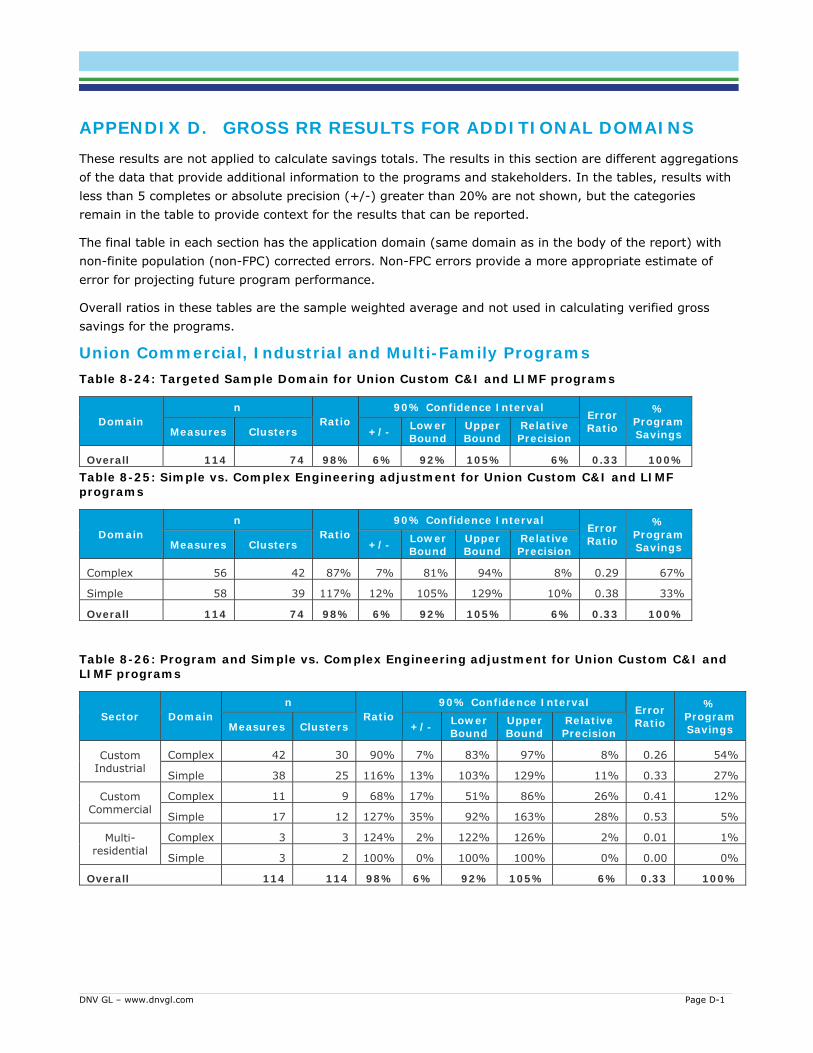
DNV GL – www.dnvgl.com Page D-1
APPENDIX D. GROSS RR RESULTS FOR ADDITIONAL DOMAINS These results are not applied to calculate savings totals. The results in this section are different aggregations of the data that provide additional information to the programs and stakeholders. In the tables, results with less than 5 completes or absolute precision (+/-) greater than 20% are not shown, but the categories remain in the table to provide context for the results that can be reported.
The final table in each section has the application domain (same domain as in the body of the report) with non-finite population (non-FPC) corrected errors. Non-FPC errors provide a more appropriate estimate of error for projecting future program performance.
Overall ratios in these tables are the sample weighted average and not used in calculating verified gross savings for the programs.
Union Commercial, Industrial and Multi-Family Programs Table 8-24: Targeted Sample Domain for Union Custom C&I and LIMF programs
Domain n
Ratio 90% Confidence Interval
Error Ratio
% Program Savings Measures Clusters +/- Lower
Bound Upper Bound
Relative Precision
Overall 114 74 98% 6% 92% 105% 6% 0.33 100% Table 8-25: Simple vs. Complex Engineering adjustment for Union Custom C&I and LIMF programs
Domain n
Ratio 90% Confidence Interval
Error Ratio
% Program Savings Measures Clusters +/- Lower
Bound Upper Bound
Relative Precision
Complex 56 42 87% 7% 81% 94% 8% 0.29 67%
Simple 58 39 117% 12% 105% 129% 10% 0.38 33%
Overall 114 74 98% 6% 92% 105% 6% 0.33 100%
Table 8-26: Program and Simple vs. Complex Engineering adjustment for Union Custom C&I and LIMF programs
Sector Domain n
Ratio 90% Confidence Interval
Error Ratio
% Program Savings Measures Clusters +/- Lower
Bound Upper Bound
Relative Precision
Custom Industrial
Complex 42 30 90% 7% 83% 97% 8% 0.26 54%
Simple 38 25 116% 13% 103% 129% 11% 0.33 27%
Custom Commercial
Complex 11 9 68% 17% 51% 86% 26% 0.41 12%
Simple 17 12 127% 35% 92% 163% 28% 0.53 5%
Multi-residential
Complex 3 3 124% 2% 122% 126% 2% 0.01 1%
Simple 3 2 100% 0% 100% 100% 0% 0.00 0%
Overall 114 114 98% 6% 92% 105% 6% 0.33 100%

DNV GL – www.dnvgl.com Page D-2
Table 8-27: Detailed Measures for Union Custom C&I and LIMF programs
Domain n
Ratio 90% Confidence Interval
Error Ratio
% Program Savings Measures Clusters +/- Lower
Bound Upper Bound
Relative Precision
Hydronic Insulation 9 9 116% 11% 105% 127% 9% 0.15 8%
Heat Recovery 13 10 106% 10% 96% 117% 10% 0.17 20%
Greenhouse 15 9 92% 4% 88% 95% 4% 0.06 29%
Operational Improvements 9 7 90% 10% 80% 99% 11% 0.15 4%
Leak Repair 7 4 130% 32% 98% 162% 25% 0.21 6%
HVAC 10 10 85% 41% 44% 125% 48% 0.83 11%
Steam Trap 9 8 85% 1% 84% 86% 1% 0.02 3%
Other Action 2 1 191% 0% 0% 0% 0% 0.00 3%
Controls 10 9 82% 9% 74% 91% 11% 0.17 5%
Building Shell 8 6 99% 12% 87% 112% 12% 0.15 2%
Other Equipment 16 12 83% 18% 65% 101% 22% 0.42 9%
Other Multi-family 6 5 121% 8% 114% 129% 6% 0.07 1%
Overall 114 74 98% 6% 92% 105% 6% 0.33 100%
Table 8-28: Program and Detailed Measures for Union Custom C&I and LIMF programs
Sector Domain n
Ratio 90% Confidence Interval
Error Ratio
% Program Savings Meas. Clusts. +/- Lower
Bound Upper Bound
Relative Precision
Custom Industrial
Building Shell 8 6 89% 8% 81% 97% 9% 0.11 2% Controls 4 4 88% 20% 68% 108% 23% 0.19 2% Greenhouse 15 9 97% 3% 94% 100% 3% 0.05 29% Heat Recovery 13 10 105% 10% 95% 114% 9% 0.16 20% HVAC 5 5 93% 12% 81% 106% 13% 0.14 2% Hydronic Insulation 9 9 116% 11% 105% 127% 9% 0.15 8% Leak Repair 7 4 121% 30% 92% 151% 24% 0.21 6% Operational Improvements 9 7 96% 8% 88% 105% 9% 0.12 4% Steam Trap 3 3 100% 1% 99% 101% 1% 0.00 2% Other Equipment 7 5 70% 25% 45% 95% 35% 0.37 6%
Custom Commercial
Controls 6 5 98% 4% 93% 102% 4% 0.05 3% HVAC 5 5 59% 25% 34% 84% 42% 0.44 9% Steam Trap 6 5 99% 3% 97% 102% 3% 0.03 1% Other Action 2 1 173% 0% 0% 0% 0% 0.00 3% Other Equipment 9 7 90% 11% 79% 101% 12% 0.17 2%
Multi-Family Other 9 7 90% 11% 79% 101% 12% 0.17 2%
Overall 114 114 98% 6% 92% 105% 6% 0.33 100%

DNV GL – www.dnvgl.com Page D-3
Table 8-29: Applied Domains with non-FPC Errors for Union Custom C&I and LIMF programs
Sector Domain n
Ratio 90% Confidence Interval Error
Ratio %
Program Savings
Measures Clusters +/- Lower Bound
Upper Bound
Relative Precision
Custom Industrial
Greenhouse Equipment 15 9 92% 5% 87% 97% 6% 0.09 29%
Action 20 12 108% 20% 88% 127% 18% 0.35 12%
Hydronic Insulation 9 9 116% 15% 101% 131% 13% 0.21 8%
Other Equipment 36 25 101% 20% 81% 120% 19% 0.57 33% Custom Commercial and LIMF 34 24 89% 30% 59% 120% 34% 0.98 19%
Overall 114 74 99% 9% 89% 108% 10% 0.49 100%

DNV GL – www.dnvgl.com Page D-4
Union Large Volume Table 8-30: Simple vs. Complex Engineering adjustment for Union Large Volume
Domain
n
Ratio
90% Confidence Interval Error Ratio
% Program Savings
Measures Clusters +/- Lower
Bound Upper Bound
Relative Precisio
n
Complex 55 24 102% 20% 82% 122% 20% 0.57 49%
Simple 22 15 57% 23% 33% 80% 41% 0.91 51%
Overall 77 36 78% 20% 58% 98% 26% 0.91 100%
Table 8-31: Detailed Measures for Union Large Volume
Domain n
Ratio 90% Confidence Interval
Error Ratio
% Program Savings Measures Clusters +/- Lower
Bound Upper Bound
Relative Precision
Hydronic Insulation 6 5 99% 2% 97% 100% 2% 0.02 44%
Heat Recovery 13 10 140% 57% 83% 196% 41% 0.70 8%
Operational Improvements 15 10 56% 12% 45% 68% 21% 0.36 19%
Leak Repair 18 11 46% 24% 23% 70% 51% 0.93 7%
Steam Trap 14 9 62% 34% 28% 96% 54% 0.88 4%
Other Action 3 3 96% 28% 67% 124% 30% 0.18 5%
Other Equipment 8 7 122% 109% 13% 232% 89% 1.22 13%
Overall 77 36 78% 20% 58% 98% 26% 0.91 100%
Table 8-32: Applied Domains with non-FPC Errors for Union Large Volume
Domain n
Ratio 90% Confidence Interval Error
Ratio %
Program Savings
Measures Clusters +/- Lower Bound
Upper Bound
Relative Precision
Equipment 24 18 116% 36% 80% 152% 31% 0.76 68%
Action 53 18 175% 176% -1% 350% 101% 2.45 32%
Overall 77 36 135% 81% 54% 217% 60% 2.13 100%

DNV GL – www.dnvgl.com Page D-5
Enbridge Commercial, Industrial and Multi-Residential Programs Table 8-33: Targeted Sampling Domains for Enbridge Custom C&I and LIMF programs
Domain
n
Ratio 90% Confidence Interval
Error Ratio
% Program Savings
Measures Customers +/- Lower Bound
Upper Bound
Relative Precision
Custom Industrial 53 41 100% 3% 97% 103% 3% 0.12 39% Custom Commercial and LIMF 74 41 91% 14% 78% 105% 15% 0.57 61%
Overall 127 82 95% 9% 86% 103% 9% 0.51 100% Table 8-34: Simple vs. Complex Engineering adjustment for Enbridge Custom C&I and LIMF programs
Domain n
Ratio 90% Confidence Interval
Error Ratio
% Program Savings Measures Clusters +/- Lower
Bound Upper Bound
Relative Precision
Complex 64 41 100% 3% 97% 103% 3% 0.12 41% Simple 63 45 92% 14% 78% 106% 15% 0.61 59%
Overall 127 82 95% 9% 86% 103% 9% 0.51 100%
Table 8-35: Program and Simple vs. Complex Engineering adjustment for Enbridge Custom C&I and LIMF programs
Sector Domain n
Ratio 90% Confidence Interval
Error Ratio
% Program Savings Measures Clusters +/- Lower
Bound Upper Bound
Relative Precision
Custom Industrial
Simple 37 26 100% 4% 96% 104% 4% 0.11 33%
Complex 16 16 102% 2% 101% 104% 2% 0.04 7%
Custom Commercial
Simple 22 14 82% 27% 56% 109% 33% 0.69 30%
Complex 14 9 100% 7% 93% 107% 7% 0.11 6%
Multi-residential
Simple 25 15 104% 4% 100% 108% 4% 0.09 22%
Complex 13 6 99% 2% 97% 101% 2% 0.02 2%
Overall 127 82 95% 9% 86% 103% 9% 0.51 100%

DNV GL – www.dnvgl.com Page D-6
Table 8-36: Detailed Measures for Enbridge Custom C&I and LIMF programs
Domain n
Ratio 90% Confidence Interval
Error Ratio
% Program Savings Measures Clusters +/- Lower
Bound Upper Bound
Relative Precision
Heat Recovery 13 10 98% 5% 93% 103% 5% 0.09 9% Etools Boiler 18 12 104% 3% 101% 107% 3% 0.06 25% Etools Ventilation 16 15 100% 3% 96% 103% 4% 0.08 21% Steam Trap 21 13 124% 2% 122% 126% 1% 0.03 4% Etools Boiler Add-on 8 7 101% 15% 86% 116% 15% 0.20 3% Other Equipment 29 23 74% 27% 47% 101% 37% 1.03 34% Other Action 3 3 20% 16% 4% 36% 80% 0.47 0% Other Multi-Residential 19 9 101% 2% 99% 103% 2% 0.03 4%
Overall 127 82 95% 9% 86% 103% 9% 0.51 100%
Table 8-37: Program and Detailed Measures for Enbridge Custom C&I and LIMF programs
Sector Domain n
Ratio 90% Confidence Interval
Error Ratio
% Program Savings Measures Clusters +/- Lower
Bound Upper Bound
Relative Precision
Custom Industrial
Etools Ventilation 4 3 106% 8% 97% 114% 8% 0.05 10% Heat Recovery 12 9 99% 5% 94% 104% 5% 0.08 9% Steam Trap 8 8 106% 3% 104% 109% 2% 0.04 2% Other Action 3 3 32% 25% 8% 57% 76% 0.45 0% Other Equipment 25 19 94% 6% 88% 99% 6% 0.15 18%
Custom Commercial
Etools Boiler 3 3 100% 0% 100% 100% 0% 0.00 8% Etools Boiler Add-on 8 7 106% 13% 94% 119% 12% 0.16 3% Etools Ventilation 8 8 97% 7% 90% 104% 8% 0.11 8% Steam Trap 13 5 100% 0% 100% 100% 0% 0.00 2% Other Equipment 4 4 52% 70% -18% 122% 135% 1.15 16%
Multi-residential
Etools Boiler 15 9 107% 4% 103% 110% 3% 0.06 17% Etools Ventilation 4 4 93% 11% 82% 104% 12% 0.10 4% Other Multi-Residential 19 9 100% 1% 99% 101% 1% 0.02 4%
Overall 127 82 95% 9% 86% 103% 9% 0.51 100%

DNV GL – www.dnvgl.com Page D-7
Table 8-38: Applied Domains with non-FPC Errors for Enbridge Custom C&I and LIMF programs
Sector Domain n
Ratio 90% Confidence Interval Error
Ratio %
Program Savings
Measures Clusters +/- Lower Bound
Upper Bound
Relative Precision
Custom Industrial
Heat Recovery 13 10 98% 8% 90% 106% 8% 0.14 9%
Steam Trap 8 8 128% 5% 123% 132% 4% 0.05 2%
Other 32 25 99% 7% 92% 106% 7% 0.20 28% Custom Commercial and Multi-residential 74 41 91% 15% 77% 106% 16% 0.61 61%
Overall 127 82 95% 10% 85% 104% 10% 0.55 100%

DNV GL – www.dnvgl.com Page E-1
APPENDIX E. NTG Results for Additional Domains These results are not applied to calculate savings totals. The results in this section are different aggregations of the data that provide additional information to the programs and stakeholders. In the tables, results with less than 5 completes or absolute precision (+/-) greater than 20% are not shown, but the categories remain in the table to provide context for the results that can be reported.
The final table in each section has the application domain (same domain as in the body of the report) with non-finite population (non-FPC) corrected errors. Non-FPC errors provide a more appropriate estimate of error for projecting future program performance.
Overall ratios in these tables are the sample weighted average and not used in calculating net savings for the programs.
Union Commercial, Industrial and Multi-Family Programs Table 8-39: Targeted Sample Domain for Union Custom C&I programs
Domain n
Ratio 90% Confidence Interval
Error Ratio
% Program Savings Measures Clusters +/- Lower
Bound Upper Bound
Relative Precision
Custom Industrial 136 84 38% 5% 33% 43% 13% 0.74 82% Custom Commercial 62 28 43% 11% 32% 54% 26% 0.80 18%
Overall 198 112 39% 5% 34% 44% 12% 0.76 100%
Table 8-40: Net-to-Gross Category for Union Custom C&I programs
Domain n
Ratio 90% Confidence Interval
Error Ratio
% Program Savings Measures Clusters +/- Lower
Bound Upper Bound
Relative Precision
Equipment 147 85 41% 5% 36% 46% 12% 0.67 80%
Action 49 26 35% 12% 22% 47% 35% 1.06 19%
Multi-family * * * 0% * * 0% 0.00 1%
Overall 198 112 39% 5% 34% 44% 12% 0.76 100%
Table 8-41: Program and Net-to-Gross Category for Union Custom C&I programs
Sector Domain n
Ratio 90% Confidence Interval
Error Ratio
% Program Savings Measures Clusters +/- Lower
Bound Upper Bound
Relative Precision
Custom Industrial
Equipment 107 67 42% 5% 36% 47% 13% 0.64 70%
Action 29 17 24% 12% 11% 36% 52% 1.23 12%
Custom Commercial
Equipment 40 18 33% 4% 29% 37% 11% 0.27 11%
Action * * * 21% * * 36% 0.58 7%
Multi-family Multi-family * * * 0% * * 0% 0.00 1%
Overall 198 112 39% 5% 34% 44% 12% 0.76 100%

DNV GL – www.dnvgl.com Page E-2
Table 8-42: Detailed Measures for Union Custom C&I programs
Domain n
Ratio 90% Confidence Interval
Error Ratio
% Program Savings Measures Clusters +/- Lower
Bound Upper Bound
Relative Precision
Hydronic Insulation 12 12 42% 13% 29% 55% 31% 0.60 8%
Heat Recovery 29 21 59% 7% 52% 66% 12% 0.32 20%
Greenhouse 26 17 40% 12% 28% 52% 30% 0.70 29%
Operational Improvements 9 7 10% 9% 1% 19% 85% 1.16 4%
Leak Repair 14 9 37% 16% 21% 52% 42% 0.68 6%
HVAC 21 17 33% 17% 16% 51% 52% 1.23 11%
Steam Trap 14 12 38% 11% 27% 48% 28% 0.55 3%
Other Action * * * 23% * * 62% 0.52 3%
Controls 23 13 45% 9% 36% 54% 20% 0.40 5%
Building Shell * * * 20% * * 38% 0.66 2%
Other Equipment 28 19 18% 9% 10% 27% 47% 1.17 9%
Other Multi-family * * * 0% * * 0% 0.00 1%
Overall 198 112 39% 5% 34% 44% 12% 0.76 100%
Table 8-43: Program and Detailed Measures for Union Custom C&I programs
Sector Domain n
Ratio 90% Confidence Interval
Error Ratio
% Program Savings Meas. Clusts +/- Lower
Bound Upper Bound
Relative Precision
Custom Industrial
Greenhouse 26 17 40% 12% 28% 52% 30% 0.70 29%
Heat Recovery 29 21 59% 7% 52% 66% 12% 0.32 20% Hydronic Insulation 12 12 42% 13% 29% 55% 31% 0.60 8%
Leak Repair 14 9 37% 16% 21% 52% 42% 0.68 6% Operational Improvements 9 7 10% 9% 1% 19% 85% 1.16 4%
Building Shell * * * 20% * * 38% 0.66 2%
Controls 7 7 18% 4% 14% 22% 21% 0.29 2%
Steam Trap 6 6 29% 12% 17% 41% 42% 0.52 2%
HVAC * * * 21% * * 95% 1.64 2%
Other 10 8 7% 8% -1% 15% 108% 1.61 6%
Custom Commercial
HVAC 10 7 46% 19% 27% 65% 41% 0.56 9%
Controls 16 6 78% 5% 74% 83% 6% 0.07 3%
Steam Trap 8 6 54% 16% 38% 69% 29% 0.35 1%
Other Action * * * 23% * * 62% 0.52 3% Other Equipment 18 11 38% 8% 30% 46% 20% 0.37 2%
Multi-Family Other * * * 0% * * 0% 0.00 1%
Overall 198 112 39% 5% 34% 44% 12% 0.76 100%

DNV GL – www.dnvgl.com Page E-3
Table 8-44: Applied Domains with non-FPC Errors for Union Custom C&I programs
Sector Domain n
Ratio 90% Confidence Interval Error
Ratio %
Program Savings
Measures Customers +/- Lower Bound
Upper Bound
Relative Precision
Custom Industrial
Greenhouse 26 17 38% 27% 11% 65% 71% 1.68 29%
Heat Recovery 29 21 58% 17% 41% 74% 29% 0.76 20%
Leak Repair and Hydronic Insulation 26 21 35% 19% 17% 54% 53% 1.41 14% Operational Improvements 9 7 12% 15% -3% 27% 123% 1.68 4%
Controls 7 7 19% 8% 11% 26% 41% 0.56 2%
Steam Trap 6 6 29% 21% 8% 50% 73% 0.89 2%
Other 33 23 21% 19% 2% 40% 90% 2.51 10%
Custom Commercial
Controls 16 6 78% 39% 39% 117% 50% 0.61 3%
Other 46 23 42% 32% 10% 75% 76% 2.13 16%
Overall 198 112 38% 10% 28% 49% 27% 1.70 100%

DNV GL – www.dnvgl.com Page E-4
Union Large Volume Table 8-45: Net-to-Gross Category for Union Large Volume
Domain n
Ratio 90% Confidence Interval
Error Ratio
% Program Savings Measures Clusters +/- Lower
Bound Upper Bound
Relative Precision
Equipment 26 21 5% 2% 3% 7% 37% 0.98 68%
Action 57 20 12% 4% 8% 16% 34% 0.89 32%
Overall 83 41 8% 2% 6% 10% 27% 1.02 100%
Table 8-46: Detailed Measures for Union Large Volume
Domain n
Ratio 90% Confidence Interval
Error Ratio
% Program Savings Measures Clusters +/- Lower
Bound Upper Bound
Relative Precision
Hydronic Insulation 10 7 6% 3% 3% 9% 51% 0.70 44%
Heat Recovery 13 10 7% 5% 2% 11% 70% 1.20 8%
Operational Improvements 20 12 13% 5% 7% 18% 41% 0.79 19%
Leak Repair 14 8 12% 6% 5% 18% 55% 0.82 7%
Steam Trap 17 11 21% 7% 13% 28% 35% 0.65 4%
Other Equipment 6 6 0% 0% 0% 0% 146% 1.77 13%
Other Action * * * 0% * * 0% 0.00 5%
Overall 83 41 8% 2% 6% 10% 27% 1.02 100%
Table 8-47: Applied Domains with non-FPC Errors for Union Custom C&I programs
Domain n
Ratio 90% Confidence Interval Error
Ratio %
Program Savings
Measures Customers +/- Lower Bound
Upper Bound
Relative Precision
Hydronic Insulation 10 7 6% 12% -7% 18% 217% 2.95 44% Operational Improvements 20 12 17% 11% 6% 29% 67% 1.28 19%
Heat Recovery 13 10 11% 15% -5% 26% 144% 2.48 8% Leak Repair and Other Actions 17 11 7% 9% -2% 15% 127% 2.33 12%
Steam Trap 17 11 21% 17% 4% 38% 83% 1.52 4% Other Equipment 6 6 0% 0% 0% 0% 235% 2.86 13%
Overall 83 41 11% 6% 5% 17% 58% 2.21 100%

DNV GL – www.dnvgl.com Page E-5
Enbridge Commercial, Industrial and Multi-Residential Programs Table 8-48: Targeted Sample Domain for Enbridge Custom C&I programs
Domain n
Ratio 90% Confidence Interval
Error Ratio
% Program Savings Measures Clusters +/- Lower
Bound Upper Bound
Relative Precision
Custom Industrial 60 50 32% 5% 27% 37% 15% 0.65 42%
Custom Commercial 101 62 27% 7% 20% 35% 26% 1.20 58%
Overall 161 112 29% 4% 25% 34% 15% 0.97 100%
Table 8-49: Net-to-Gross Category for Enbridge Custom C&I programs
Domain n
Ratio 90% Confidence Interval
Error Ratio
% Program Savings Measures Clusters +/- Lower
Bound Upper Bound
Relative Precision
Equipment 102 79 26% 4% 21% 30% 16% 0.87 76%
Action 24 16 25% 13% 12% 37% 51% 1.17 5%
Multi-Residential 35 17 44% 14% 30% 58% 31% 0.74 19%
Overall 161 112 29% 4% 25% 34% 15% 0.97 100%
Table 8-50: Program and Net-to-Gross Category for Enbridge Custom C&I programs
Sector Domain n
Ratio 90% Confidence Interval
Error Ratio
% Program Savings Measures Clusters +/- Lower
Bound Upper Bound
Relative Precision
Custom Industrial
Equipment 50 40 33% 5% 28% 38% 15% 0.56 40%
Action 10 10 * 22% * * 96% 1.65 3%
Custom Commercial
Equipment 52 39 17% 7% 10% 24% 40% 1.47 37%
Action 14 6 27% 5% 22% 33% 19% 0.23 2% Multi-
Residential Multi-Residential 35 17 44% 14% 30% 58% 31% 0.74 19%
Overall 161 112 29% 4% 25% 34% 15% 0.97 100%

DNV GL – www.dnvgl.com Page E-6
Table 8-51: Detailed Measures for Enbridge Custom C&I programs
Domain n
Ratio 90% Confidence Interval
Error Ratio
% Program Savings Measures Clusters +/- Lower
Bound Upper Bound
Relative Precision
Heat Recovery 13 10 55% 9% 46% 64% 16% 0.27 10%
Etools Ventilation 30 29 12% 5% 7% 17% 43% 1.36 22%
Etools Boiler 24 19 27% 10% 17% 36% 36% 0.90 21%
Steam Trap 24 16 25% 13% 12% 37% 51% 1.17 4%
Etools Boiler Add-on 11 9 14% 4% 10% 18% 29% 0.46 3%
Other Equipment 42 33 28% 7% 21% 35% 25% 0.83 36%
Other Multi-Residential 17 7 97% 3% 94% 100% 3% 0.05 3%
Overall 161 112 29% 4% 25% 34% 15% 0.97 100%
Table 8-52: Program and Detailed Measures for Enbridge Custom C&I programs
Sector Domain n
Ratio 90% Confidence Interval
Error Ratio
% Program Savings Measures Clusters +/- Lower
Bound Upper Bound
Relative Precision
Custom Industrial
Etools Ventilation 8 7 15% 10% 5% 25% 70% 0.95 10% Heat Recovery 13 10 55% 9% 46% 64% 16% 0.27 10% Steam Trap * * * 22% * * 96% 1.65 2% Other Equipment 29 24 33% 7% 25% 40% 23% 0.65 19%
Custom Commercial
Etools Ventilation 15 15 5% 4% 1% 8% 72% 1.58 8% Etools Boiler 13 11 27% 15% 12% 41% 54% 0.99 8% Boiler Add-on 11 9 14% 4% 10% 18% 29% 0.46 3% Steam Trap 14 6 27% 5% 22% 33% 19% 0.23 2%
Other 13 9 18% 12% 5% 30% 70% 1.13 17%
Multi-Residential
Etools Boiler 11 8 26% 14% 12% 40% 54% 0.80 13% Etools Ventilation 7 7 20% 14% 6% 34% 71% 0.97 3%
Other 17 7 97% 3% 94% 100% 3% 0.05 3%
Overall 161 112 29% 4% 25% 34% 15% 0.97 100%

DNV GL – www.dnvgl.com Page E-7
Table 8-53: Applied Domains with non-FPC Errors for Enbridge Custom C&I programs
Sector Domain n
Ratio 90% Confidence Interval Error
Ratio %
Program Savings
Measures Customers +/- Lower Bound
Upper Bound
Relative Precision
Custom Industrial
Etool Ventilation 8 7 15% 22% -7% 37% 146% 1.98 10% Heat Recovery 13 10 55% 30% 25% 85% 54% 0.93 10%
Other 39 34 31% 18% 14% 49% 56% 1.95 22%
Custom Commercial
Etool Ventilation 15 15 5% 5% 0% 9% 91% 2.01 8% Etool Boiler and Boiler Add-on 25 20 23% 14% 9% 37% 61% 1.57 12% Steam Trap 14 6 27% 14% 13% 42% 52% 0.63 2%
Other 12 8 21% 20% 1% 42% 97% 1.45 16%
Multi-Residential
Etool Boiler 11 8 27% 16% 10% 43% 61% 0.90 13% Etool Ventilation 7 7 20% 21% -2% 41% 108% 1.47 3%
Other 17 7 97% 4% 93% 101% 4% 0.06 3%
Overall 161 112 29% 9% 21% 38% 29% 1.87 100%
RunitRight Table 8-54: Net-to-Gross Category for Enbridge RunitRight
Domain n
Ratio 90% Confidence Interval
Error Ratio
% Program Savings Measures Clusters +/- Lower
Bound Upper Bound
Relative Precision
Action 16 10 50% 14% 36% 64% 27% 0.47 100%
Overall 16 10 50% 14% 36% 64% 27% 0.47 100%
Table 8-55: Applied Domains with non-FPC Errors for Enbridge RunitRight
Domain n
Ratio 90% Confidence Interval Error
Ratio %
Program Savings
Measures Customers +/- Lower Bound
Upper Bound
Relative Precision
RunitRight 16 10 50% 20% 30% 70% 39% 0.68 100%

DNV GL – www.dnvgl.com Page F-1
APPENDIX F. SECONDARY ATTRIBUTION Results These results are not applied to calculate savings totals. This secondary attribution approach is lower rigour than the primary approach and provides a sense of the incremental effect that historical program efforts have on projects today. This score is not intended for application in determining program net savings.
Union Commercial, Industrial and Multi-Family Programs Table 8-56: Secondary Attribution for Union Custom C&I programs
Sector Domain n Secondary
Attr Ratio Ratio Ratio Difference % Program
Savings Measures Clusters
Custom Industrial
Greenhouse 26 17 46% 40% 6% 29%
Heat Recovery 29 21 61% 59% 2% 20% Leak Repair and Hydronic Insulation 26 21 54% 40% 14% 14% Operational Improvements 9 7 10% 10% 0% 4%
Controls 7 7 51% 18% 32% 2%
Steam Trap 6 6 35% 29% 7% 2%
Other 33 23 21% 21% 0% 10%
Custom Commercial
Controls 16 6 92% 78% 14% 3%
Other 46 23 45% 38% 7% 16%
Overall 198 112 45% 39% 6% 100%
Union Large Volume Table 8-57: Secondary Attribution for Union Large Volume
Domain n Secondary
Attr Ratio Ratio Ratio Difference
% Program Savings Measures Clusters
Hydronic Insulation 10 7 6% 6% 0% 44% Operational Improvements 20 12 21% 13% 8% 19%
Heat Recovery 13 10 15% 7% 9% 8%
Steam Trap 17 11 21% 21% 1% 4%
Other Equipment 6 6 1% 0% 1% 13% Leak Repair and Other Actions 17 11 17% 9% 8% 12%
Overall 83 41 12% 8% 4% 100%

DNV GL – www.dnvgl.com Page F-2
Enbridge Commercial, Industrial and Multi-Residential Programs Table 8-58: Secondary Attribution for Enbridge Custom C&I programs
Sector Domain n Secondary
Attr Ratio Ratio Ratio Difference
% Program Savings Measures Clusters
Custom Industrial
Etools Ventilation 8 7 15% 15% 0% 10%
Heat Recovery 13 10 61% 55% 6% 10%
Other 39 34 39% 31% 8% 22%
Custom Commercial
Etools Ventilation 15 15 35% 5% 31% 8%
Steam Trap 14 6 61% 27% 33% 2% Etools Boiler and Boiler Add-on 25 20 27% 24% 3% 12%
Other 12 8 24% 18% 6% 16%
Multi-Residential
Etools Boiler 11 8 30% 26% 4% 13%
Etools Ventilation 7 7 60% 20% 41% 3%
Other 17 7 99% 97% 1% 3%
Overall 161 112 39% 29% 9% 100%
RunitRight Table 8-59: Secondary Attribution for Enbridge RunitRight
Domain n Secondary
Attr Ratio Ratio Ratio Difference
% Program Savings Measures Clusters
RunitRight 16 10 60% 50% 10% 100%
Overall 16 10 60% 50% 10% 100%
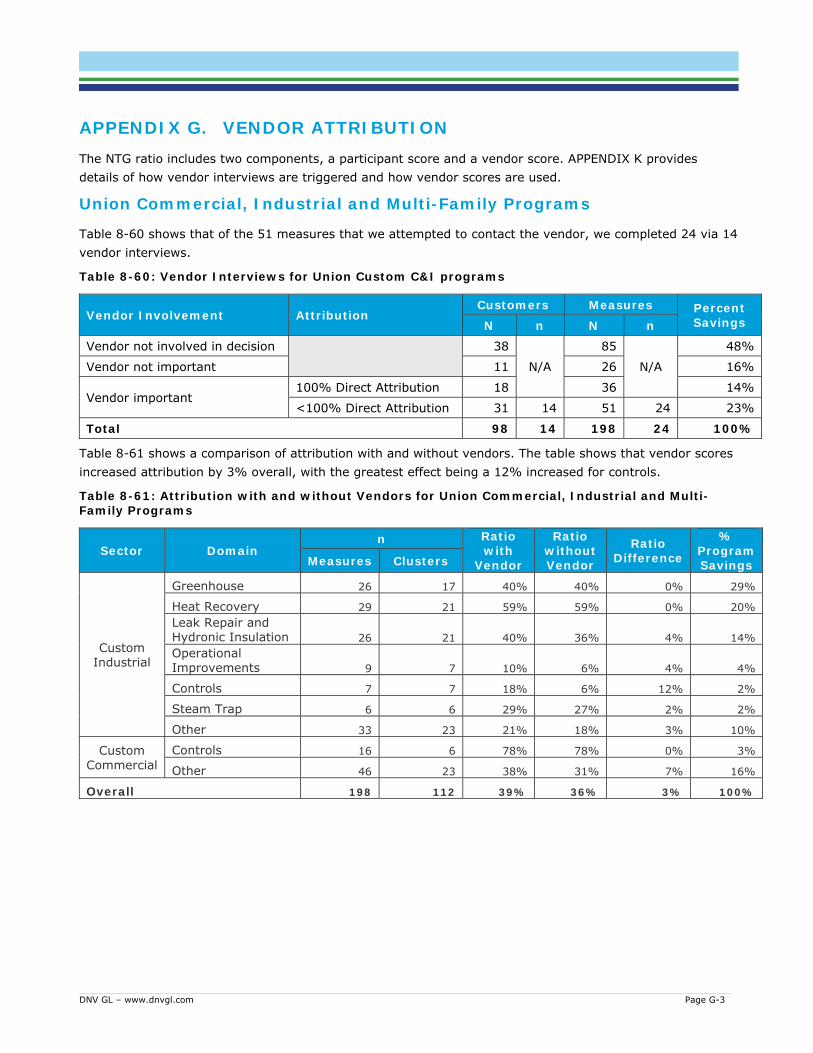
DNV GL – www.dnvgl.com Page G-3
APPENDIX G. VENDOR ATTRIBUTION The NTG ratio includes two components, a participant score and a vendor score. APPENDIX K provides details of how vendor interviews are triggered and how vendor scores are used.
Union Commercial, Industrial and Multi-Family Programs
Table 8-60 shows that of the 51 measures that we attempted to contact the vendor, we completed 24 via 14 vendor interviews.
Table 8-60: Vendor Interviews for Union Custom C&I programs
Vendor Involvement Attribution Customers Measures Percent
Savings N n N n
Vendor not involved in decision 38
N/A
85
N/A
48%
Vendor not important 11 26 16%
Vendor important 100% Direct Attribution 18 36 14%
<100% Direct Attribution 31 14 51 24 23%
Total 98 14 198 24 100%
Table 8-61 shows a comparison of attribution with and without vendors. The table shows that vendor scores increased attribution by 3% overall, with the greatest effect being a 12% increased for controls.
Table 8-61: Attribution with and without Vendors for Union Commercial, Industrial and Multi-Family Programs
Sector Domain n Ratio
with Vendor
Ratio without Vendor
Ratio Difference
% Program Savings Measures Clusters
Custom Industrial
Greenhouse 26 17 40% 40% 0% 29%
Heat Recovery 29 21 59% 59% 0% 20% Leak Repair and Hydronic Insulation 26 21 40% 36% 4% 14% Operational Improvements 9 7 10% 6% 4% 4%
Controls 7 7 18% 6% 12% 2%
Steam Trap 6 6 29% 27% 2% 2%
Other 33 23 21% 18% 3% 10%
Custom Commercial
Controls 16 6 78% 78% 0% 3%
Other 46 23 38% 31% 7% 16%
Overall 198 112 39% 36% 3% 100%

DNV GL – www.dnvgl.com Page G-4
Union Large Volume
Table 8-62 shows that we attempted to contact five vendors and were only able to complete one.
Table 8-62: Vendor Interviews for Union Large Volume
Vendor Involvement Attribution Customers N n
Vendor not involved in decision 16 N/A Vendor not important 2
Vendor important 100% Direct Attribution 11 <100% Direct Attribution 5 1
Total 34 1 For confidentiality reasons, the number of measures and percent of savings cannot be reported for this program.
Table 8-63 shows that vendor attribution did not increase overall attribution for this program.
Table 8-63: Attribution with and without Vendors for Union Large Volume
Domain n Ratio
with Vendor
Ratio without Vendor
Ratio Difference
% Program Savings Measures Clusters
Hydronic Insulation 10 7 6% 6% 0% 44% Operational Improvements 20 12 13% 13% 0% 19% Leak Repair and Other Actions 17 11 9% 9% 0% 12% Heat Recovery 13 10 7% 7% 0% 8% Steam Trap 17 11 21% 21% 0% 4% Other Equipment 6 6 0.1% 0.1% 0% 13% Overall 83 41 8% 8% 0% 100%

DNV GL – www.dnvgl.com Page G-5
Enbridge Commercial, Industrial and Multi-Residential Programs
Table 8-64 shows that of the 49 measures that we attempted to contact the vendor, we completed 23 via 19 vendor interviews.
Table 8-64: Vendor Interviews for Enbridge Custom C&I programs
Vendor Involvement Attribution Customers Measures Percent
Savings N n N n Vendor not involved in decision 27
N/A 50
N/A 31%
Vendor not important 6 9 9%
Vendor important 100% Direct Attribution 29 54 30% <100% Direct Attribution 37 19 49 23 30%
Total 99 19 162 23 100%
Table 8-65 shows that vendor attribution increased overall program attribution by 2%. The greatest increases were for Multi-residential boilers and ventilation.
Table 8-65: Attribution with and without Vendors for Enbridge Custom C&I programs
Sector Domain n Ratio
with Vendor
Ratio without Vendor
Ratio Difference
% Program Savings Measures Clusters
Custom Industrial
Etools Ventilation 8 7 15% 15% 0% 10% Heat Recovery 13 10 55% 55% 0% 10% Other 39 34 31% 30% 1% 22%
Custom Commercial
Etools Ventilation 15 15 5% 5% 0% 8% Steam Trap 14 6 27% 27% 0% 2% Etools Boiler and Boiler Add-on 25 20 24% 22% 2% 12% Other 12 8 18% 16% 2% 16%
Multi-Residential
Etools Boiler 11 8 26% 19% 7% 13% Etools Ventilation 7 7 20% 11% 8% 3% Other 17 7 97% 97% 0% 3%
Overall 161 112 29% 28% 2% 100%
RunitRight
Table 8-66 shows that we attempted to contact two vendors and were only able to complete one.
Table 8-66: Vendor Interviews for Enbridge RunitRight
Vendor Involvement Attribution Customers N n
Vendor not involved in decision 3 N/A Vendor not important 1
Vendor important 100% Direct Attribution 1 <100% Direct Attribution 2 1
Total 7 1 For confidentiality reasons, the number of measures and percent of savings cannot be reported for this program.
Table 8-67 shows that vendor attribution did not increase overall attribution for this program.

DNV GL – www.dnvgl.com Page G-6
Table 8-67: Attribution with and without Vendors for Enbridge RunitRight
Domain n Ratio
with Vendor
Ratio without Vendor
Ratio Difference
% Program Savings Measures Clusters
RunitRight 16 10 50% 50% 0% 100%
Overall 16 10 50% 50% 0% 100%

DNV GL – www.dnvgl.com Page H-7
APPENDIX H. MAPPING OF REPORTING DOMAINS TO TRACKING CATEGORIES
A map of reporting domains to tracking database records and categorization will be provided to each utility in Excel format to facilitate adding the ratio results to their internal data.

DNV GL – www.dnvgl.com Page I-1
APPENDIX I. SAMPLING PROCESS This appendix provides detail on the:
High-level process used in sampling exploration of tracking data definition of the unit of analysis stratification decisions 2015 FR and CPSV sample design 2013/14 Spillover Sample design Sample and backup sample selection
High-level process
A sample is a collection of data items such as those collected through surveys, metering or on-site observation. A sample design is required when a sample does not include the entire target population. Most sample designs are driven by cost constraints (including schedule constraints), desired precision or both. The sampling process described here ensures that all bases are covered, ensuring optimal precision around estimates of interest for the data collected. The process we followed is detailed below. All numbers and observations and goals described were operating assumptions used at the beginning of the process:
1. Identify Goals, Methods and Constraints: for sampling, the goals consist of identifying the primary and secondary estimates of interest: what quantitative results are most important. Defining the data collection methodology –the process used to gather the data for the analysis – and the estimation method – the approach used to calculate the primary estimate of interest – is critical for defining elements of the design. Cost and schedule constraints surrounding the data collection and analysis then determine an upper bound for the sample size.
- Goals: For this study the primary estimate of interest is the NTG ratio for each program. The NTG ratio is the parameter that we are targeting for 90/10 precision for each program.
As will be described later in the methodology memo, we calculate the NTG ratio as
NTG = (1-FR)*(1+SO).
Since spillover tends to be small, this formulation is mathematically very close to the simpler formula indicated in the recent Ontario evaluations
NTG = 1-FR + SO.
We prefer the multiplicative formula as a more complete expression of the relationship between free ridership and spillover.
Previous work in Ontario indicates that free ridership is on the order of 10% to 60% across program segments, 50% overall on a savings-weighted basis. Spillover is on the order of 5%. Because spillover is generally small, the precision of the full NTG will in most cases be close to that of the net-of-free rider factor, even with a modest spillover sample size.
- Methods and Constraints: We are using two data collection methods, each of which have different costs associated. Due to cost constraints we must limit our use of on-sites to those projects where it

DNV GL – www.dnvgl.com Page I-2
will make the most difference in the estimate. These will be deployed on the largest and most complex projects as identified based on tracking data descriptions. TSERs will be used to collect the balance of the data that we do not have the funds to collect with On-sites. For smaller and simpler projects where the decisions made are more straight forward, TSER verification provides accurate data at a reasonable cost.
Define the unit of analysis: The unit of analysis is the level at which final estimates will be made. Some studies have multiple units of analysis: process evaluation results may be based on respondent level estimates, while impact evaluation results may be based on measure or project level estimates. Sampling units do not need to be the same as the unit of analysis, but identifying both early is crucial.
We are using the same definition for our sampling unit. Most customers have no more than three projects in a given year, and most projects are of only one or two measure types, so that we will be able to inquire about all of these in a single survey or interview of reasonable length.
We plan to ask each sampled customer about attribution for all of the customer’s measures. Only a handful of customers have more than three (unit of analysis level) measures in 2016, with a maximum of six.
For customers with large numbers of projects and measures, we will ask about groups of measures or projects. The groupings will depend on details of the types of measures and savings magnitudes.
Identify the target population: The target population is the universe of items that inferences and estimates are desired for. In the initial scope of the NTG study, the primary target population was defined as future programs of the same type. Having future program years as the target population has two implications for the sample design. First, the applicable error associated with our estimates is the non-finite population corrected error (described in our discussion of sample size below) which requires larger sample sizes for a given precision. Second, analysis by sub-domains such as measure types within the programs becomes more important. The measure mix in programs changes from year to year and typically NTG varies more across measure types than within. For more accurate estimates of net savings for future program years, applying measure type NTG ratios will be preferred to program as a whole NTG ratios. At this time the question of prospective vs. retrospective application of NTG results is unresolved. The final sample design is expected to result in precision levels sufficient for either application of the results.
Establish the Sample Frame: The sample frame refers to the list or mechanism from which the sample is drawn. A perfect frame will match the target population exactly.
Since the target populations of this study are the future programs, we will not have a perfect sample frame; however, if the program designs remain relatively stable, using past program participants as the sample frame will provide a good list from which to draw our sample.
Determine sample size: Sample size refers to the number of items that are selected from the sample frame in order to draw inferences and create estimates about the target population. In stratified designs, sample sizes are determined for each stratum.
Critical to the sample size determination is the error ratio for each sampling cell with respect to the ratio to the estimated. The error ratio for ratio estimation is the equivalent of the coefficient of variation for estimation of a population mean. Our experience with conducting similar NTG studies of

DNV GL – www.dnvgl.com Page I-3
commercial-industrial customers is that the error ratio for the free rider rate is between 0.7 and 0.8 within reasonably defined sampling cells.
In determining these sample sizes, the number of customers in the full population is also important for two reasons. First, if we are trying to estimate a parameter for a finite population, the sample size required is reduced by the Finite Population Correction or FPC. Second, we need to consider the number of completed surveys we can realistically complete given likely response rates.
Use of the FPC is appropriate when the parameter of interest represents a particular population. This situation applies when we are determining the free ridership factor or spillover rate for a particular program and time frame. When we determine these factors for all future theoretical projects, it is arguably more appropriate to treat the sample drawn from recent participants as coming from an essentially infinite population. Thus, for projection to future years we generally recommend against applying the FPC.
Stratification: Stratification is the partitioning of a target population. Stratification is discussed in depth in the sample design section in the body of the Scope of Work.
Sample Selection: Sample selection refers to the process of obtaining the sample of units from the sample frame. If all units on the sample frame are selected then the design is referred to as a census or certainty sample. Otherwise units may be selected either randomly or non-randomly, depending on the evaluation goals, constraints and amount of acceptable bias. The sample selection process is a critical feature of the sample design and has a direct impact on the expected precision and bias of estimates. The optimal sample selection process for a particular project can vary greatly.
Unit and Item non-response Unit and item nonresponse are potential sources of bias, depending on the nonresponse mechanism and the level of nonresponse encountered. Unit nonresponse refers to the absence of information from an entire sampled unit. Item nonresponse refers to the situation where some data are collected, but not all, from a sampled unit. The nonresponse mechanism refers to the process that is causing the nonresponse. If the probability of responding depends on the data items being sought then the nonresponse mechanism is said to be non-ignorable. Otherwise it is called an ignorable nonresponse mechanism. Nonresponse bias tends to be greater when the nonresponse mechanism is non-ignorable and as levels of item nonresponse increase.
There are various ways to address nonresponse in a sample. For example, weight adjustments are often used to account for unit nonresponse and item imputation techniques are often used to account for item nonresponse.
If nonresponse levels are low and the response mechanism is thought to be ignorable then one could ignore nonresponse and simply create estimates among the respondents.
We recommend treating unit nonresponse as ignorable for this study since it does not depend on the data items being sought. Instead, it depends on the willingness of the decision maker at the participating business agreeing to respond to the survey.
For item nonresponse in the scored portion of the surveys we recommend treating the nonresponse as non-ignorable if all three of the T, E, Q portions of the free ridership sequence contain non-response. Otherwise we plan to treat the item nonresponse as ignorable and will impute the average response for the missing item from among scored units of the same measure type and utility. The exception to this
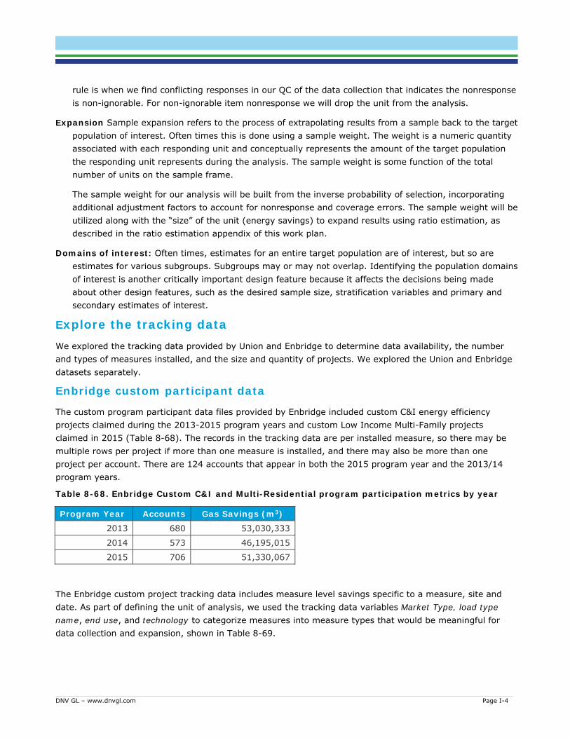
DNV GL – www.dnvgl.com Page I-4
rule is when we find conflicting responses in our QC of the data collection that indicates the nonresponse is non-ignorable. For non-ignorable item nonresponse we will drop the unit from the analysis.
Expansion Sample expansion refers to the process of extrapolating results from a sample back to the target population of interest. Often times this is done using a sample weight. The weight is a numeric quantity associated with each responding unit and conceptually represents the amount of the target population the responding unit represents during the analysis. The sample weight is some function of the total number of units on the sample frame.
The sample weight for our analysis will be built from the inverse probability of selection, incorporating additional adjustment factors to account for nonresponse and coverage errors. The sample weight will be utilized along with the “size” of the unit (energy savings) to expand results using ratio estimation, as described in the ratio estimation appendix of this work plan.
Domains of interest: Often times, estimates for an entire target population are of interest, but so are estimates for various subgroups. Subgroups may or may not overlap. Identifying the population domains of interest is another critically important design feature because it affects the decisions being made about other design features, such as the desired sample size, stratification variables and primary and secondary estimates of interest.
Explore the tracking data We explored the tracking data provided by Union and Enbridge to determine data availability, the number and types of measures installed, and the size and quantity of projects. We explored the Union and Enbridge datasets separately.
Enbridge custom participant data
The custom program participant data files provided by Enbridge included custom C&I energy efficiency projects claimed during the 2013-2015 program years and custom Low Income Multi-Family projects claimed in 2015 (Table 8-68). The records in the tracking data are per installed measure, so there may be multiple rows per project if more than one measure is installed, and there may also be more than one project per account. There are 124 accounts that appear in both the 2015 program year and the 2013/14 program years.
Table 8-68. Enbridge Custom C&I and Multi-Residential program participation metrics by year
Program Year Accounts Gas Savings (m3)
2013 680 53,030,333
2014 573 46,195,015
2015 706 51,330,067
The Enbridge custom project tracking data includes measure level savings specific to a measure, site and date. As part of defining the unit of analysis, we used the tracking data variables Market Type, load type name, end use, and technology to categorize measures into measure types that would be meaningful for data collection and expansion, shown in Table 8-69.

DNV GL – www.dnvgl.com Page I-5
Table 8-69. Enbridge participation metrics by measure, 2013-2015
Measure Type 2013-2014 (SO) 2015 (CPSV/FR) Accounts Gas Savings (m3) Accounts Gas Savings (m3)
HVAC 636 32,807,840 380 19,105,965
Controls 337 17,821,495 175 13,868,059
Other Equipment 121 25,151,192 10 2,153,339
Operational Improvements 119 9,672,787 55 7,811,661
Heat Recovery 16 1,092,519 29 4,398,419
Steam and Hot Water 175 3,376,999 86 1,825,048
Process Heat 14 4,786,413 3 73,078
Building Shell 38 1,833,941 89 1,794,104 Greenhouse 10 2,682,162 3 300,394
Enbridge RunitRight participation data
For RunitRight, the program tracking data includes projects claimed in the 2014-2015 program years. These projects were all completed in 2013-2014; savings for a project in the program do not get claimed until after one year of site metering is complete.
Table 8-70. Enbridge RunitRight program participation metrics by year claimed
Program Year Accounts Gas Savings (m3)
2014 45 625,088 2015 28 542,442
The RunitRight program has only one measure type. It also has several projects with negative savings. Negative savings (increases in energy use) are possible results from retro-commissioning projects, sometimes due to calculation method (billing analysis based savings without weather, occupancy adjustment or production adjustment) or due to actual increases in energy use. Negative saving measures need to be handled carefully in ratio estimation: high FR on large negative savings projects can result in overall program FR <0, which is not a valid result.26 Our recommended approach to the problem is to produce and apply ratios with separate domains for positive and negative savings projects.
Union custom participant data
The participant data files provided by Union included energy efficiency projects claimed during the 2013-2015 program years. The records in the tracking data are per installed measure, so there may be multiple rows per project if more than one measure is installed, and there may also be more than one project per account. There are 67 accounts that appear in both the 2015 program year and the 2013/14 program years.
26 Free ridership on negative savings results in more program savings, rather than less.

DNV GL – www.dnvgl.com Page I-6
Table 8-71. Union participation metrics by year
Program Year Accounts Gas Savings (m3)
2013 352 369,438,742
2014 392 285,752,549
2015 462 201,620,726
We used the project type, equipment type, and project category variables in the tracking data to categorize measures. Our first step was to distill the combined information from the three fields into measure types that would be meaningful for data collection and expansion, shown in Table 8-72. The largest measure types (by cumulative savings) were maintenance, steam and hot water, and optimization.
Table 8-72. Union participation metrics by measure, 2013-2015*
Measure Type 2013-2014 2015 Accounts Gas Savings (m3) Accounts Gas Savings (m3)
Maintenance 222 255,847,232 79 37,181,863 Steam and Hot Water 161 119,657,223 91 39,229,635
Optimization 91 94,790,733 28 16,936,421
Ag and Greenhouse 149 64,895,560 73 31,875,980
Heat Recovery 86 38,174,741 52 19,797,904
Other Equipment 56 27,104,377 13 20,653,141
Controls 78 16,785,704 128 13,267,526
HVAC 48 14,885,291 49 8,829,742
Process Heat 25 13,242,538 10 4,536,172
Building Shell 152 5,599,318 68 3,597,883
New Construction 19 3,714,489 5 4,589,777 Cogeneration 4 494,085 1 1,124,682
Define the unit of analysis
Following data exploration, we defined the unit of analysis, which established the level at which data will be analyzed but not the level at which it will be collected, which is the sampling unit. We further discuss this distinction and how the sampling unit is defined in the Task 2.5 section.
The definition of the unit of analysis is one of the most important and least discussed aspects of DSM program evaluation. Consider the following four dimensions: end -use, measure type, equipment or “action,” and calculation approach. The program tracking databases include the first three dimensions and do not have an identifier for the fourth (though there may be a way to proxy it). Our example assumes that calculation type can be defined at a high level with reasonable accuracy based on existing database fields for the 2015 program year. Table 8-73 shows six measures performed at a site in a year through a program. Each of these categories could be considered a possible unit of analysis.

DNV GL – www.dnvgl.com Page I-7
Table 8-73: Example dimensions used to define a unit of analysis
Measure ID Enduse Measure Type Equipment or
Action Calc Type M1 Process Heat Boiler Action Complex M2 Process Heat Boiler Equipment Complex M3 Space Heat Boiler Action Simple M4 Space Heat Boiler Equipment Simple M5 Space Heat Furnace Action Simple M6 Space Heat Furnace Equipment Simple
The end use can be important in decision making because lowering the cost per unit produced is a different decision than lowering the cost of heating a facility or office, for example. It can also be used as a proxy for the complexity of the calculation, as process-related end uses tend to have more complex and site-specific calculation approaches. End use can be used in surveys by listing the measure types that fall into the category; however, this is not ideal for NTG as the program’s influence on decision making may differ by measure type, affecting the attribution response.
Measure type is important for surveys to aid participant recall by providing a concrete, simple description of what equipment was altered or installed. This aggregation is less appropriate for CPSV where the calculation method may differ.
Equipment or Action is a very important distinction for NTG. Continuous improvement actions, such as maintenance, operations, and optimization, have fewer barriers to implementation than equipment purchases due to lower total cost, shorter term planning horizons and often fewer approvals. Businesses typically have separate budgets for capital and operating expenses. Purchases of new or replacement equipment falls under a capital budget, while actions are usually part of the operating budget or performed by salaried employees. Capital budgets typically have long term planning and allocation, while an operating budget is by nature more flexible to conditions in a given year. The ability of programs to affect equipment and action decision making is necessarily different as well. For the unit of analysis, actions were put into three categories: maintenance, operational improvement, and optimization.
Calculation type is important for CPSV. Simple, commonly implemented measures in custom programs do not require the same depth of data collection to verify calculations and inputs as more complex measures. Simple measures also use standardized calculation approaches that reduce variance. Evaluators tend to find fewer adjustments and, even when adjustments are found, the adjustment often affects all measures of a calculation approach similarly.
In the example shown in Table 8-73, aggregating across any of the four listed dimensions is a trade-off of accuracy for increased precision, reduced customer burden and reduced evaluation costs. Not aggregating makes the same trade-off, but in reverse.
We aggregated across elements that are likely to have a lesser effect on decision making (such as type of insulation) and did not aggregate across distinctions that are likely to play a larger role in how decisions were made (such as process vs space heat).
The unit of analysis for the evaluation, presented in Figure 8-1, aggregates the data to the utility, account, year, and measure type. For Union, aggregating the tracking data to the unit of analysis reduced the number of records from 744 to 597 records for 2015 and from 1,468 to 1,091 records for 2013 to 2014. For

DNV GL – www.dnvgl.com Page I-8
Enbridge, the number of records for 2015 decreased from 955 to 858 records and for 2013 to 2014 decreased from 1,648 to 1,511 records.
Figure 8-1: Unit of analysis
For this evaluation, the unit of analysis and the sampling units are defined differently. While a unit of analysis separates units of different accounts/sites, program years or measure types, the sampling unit is specific to the customer. As an example, one Enbridge customer may have installed a new boiler in 2013 and insulation in 2014, which is two different units of analysis. Since they were installed by the same customer, however, they belong to one sampling unit. In the analysis phase, weights will be developed for each unit of analysis (account-measure type-year), but for the standard error calculation, data collected from a single customer (sample unit) will be a treated as a cluster rather than evaluated as if they are independent observations.
Once aggregated to the unit of analysis, Union had an average of 1.5 units of analysis per account in 2013 and 2014 and 1.3 units per account in 201527 while Enbridge has an average of 1.2 units per account in 2013, 2014, and in 2015. In general, Union accounts tended to have more units of analysis per account than Enbridge accounts. Only 26 Union accounts have 5 units and none had more than 5. For Enbridge, 9 accounts have 4 units and no accounts have more than 4. This will facilitate data collection, since it’s reasonable to ask about 3-4 units.
At this time we are unable to comment on the number of units per customer, because some customers will likely have multiple accounts. Customers will be defined by their contact information which will be requested along with the documentation request following submission of the scope of work.
27 We are assuming a 1:1 account to customer ratio for sampling. For the analysis, customer will be defined by contact information (phone number
primarily), which is not included in the provided tracking data.

DNV GL – www.dnvgl.com Page I-9
Stratify the NTG and CPSV data
There is a balance between having too many and too few strata.28 In sample designs, more strata allow the design to control representativeness and estimated precision along more dimensions. Having more strata does not hurt overall precision, but it can increase the sample sizes required. Each stratification level serves to improve efficiency, improve representativeness, or both.
There are four populations across which the evaluation findings will be completely separate from one another.29 These populations are defined by having separate program designs. The divisions between these populations are hard lines; none of the reported ratio results will include a mix of information across these populations. We can think of this as four evaluations using a common methodology and data collection effort:
Union Large Volume Union Custom C&I Enbridge Custom C&I Enbridge RunitRight
Within the stratification segments (see Figure 8-2 and Figure 8-3) we categorize measures to improve the efficiency and representativeness of the sample. 30 The stratification for the 2015 data collection effort balances the needs of two studies, with the CPSV sample a subset of the NTG sample. Each has differing measure categorization priorities. 31
For NTG the measure categorization most predictive of free ridership rates is whether the project is installation of efficient equipment or whether the project was an action taken with existing equipment, regardless of whether that action is maintenance or an optimization that leads to energy savings.
For CPSV the measure categorization most predictive of verification rates is a simple calculation versus one that is complex. Simple projects that follow consistent approaches and vary less from site to site typically have verification rates with lower variance than more complex projects that require more site-specific knowledge and truly custom calculations. Stratifying by rigour allows us to assign a lower ER (0.3) to the simple project strata and higher to the more complex strata (0.4 ER) which provides better sample allocation. Simple strata projects will receive a TSER verification, while complex strata projects will receive an on-site verification.
The final stratification level segments projects by the magnitude of energy savings resulting from that project. Large projects represent a greater portion of the population, so sampling them at increased rates will result in greater precision with fewer verification visits or calls. Smaller projects must also be sampled to ensure representativeness. DNV GL used cumulative savings as a measure of size for the 2015 sample designs and annual savings as a measure of size for 2013/14 sample designs. Cumulative savings were not
28 DNV GL agrees with the approaches described in “Sampling Methodology for Custom C&I Programs” which was prepared by Navigant for the TEC in
2012 and used to inform previous CPSV sample designs. Our sample design approach is consistent with the approaches recommended and follows the recommended seven step process (pages 17-23). Dan Violette, Ph.D. & Brad Rogers, M.S., MBA, Navigant Consulting, Inc. “A Sampling Methodology for Custom C&I Programs,” Prepared for: Sub-Committee of the Technical Evaluation Committee. November 12, 2012 (Revised October 28, 2014).
29 For the CPSV, LI MF will be reported with MR MF either together with Custom C&I or as a separate Multi-Family domain, depending on final sample
sizes and precisions. 30 Page 14 in the Navigant report provides an explanation of the rationale for stratification. 31 The current stratification plan has more aggregated program segment categories than were described in the original proposal. When developing the
proposal sample design, we did not have access to the data or savings amounts specific to measure types.

DNV GL – www.dnvgl.com Page I-10
provided for 2013/14.32 In terms of sample allocation, using annual savings will select longer life measures at a lower rate than would occur if cumulative savings are used.
It is important to note that the stratification used for sampling and expansion does not need to correspond directly to the level of reporting. For example, while we have chosen to use broad categories of customer segments in our stratification, this does not preclude reporting by more disaggregate customer segments.
Figure 8-2 and Figure 8-3 show the CPSV and NTG stratification for Enbridge and Union respectively.
Figure 8-2: Enbridge stratification
32 The August 4, 2016 data provided by Enbridge included cumulative savings for 2015, but not 2013 and 2014.

DNV GL – www.dnvgl.com Page I-11
Figure 8-3: Union stratification
Design the 2015 samples
Critical to the sample size determination is the error ratio for each sampling cell with respect to the ratio to be estimated. The error ratio for ratio estimation is the equivalent of the coefficient of variation for estimation of a population mean. Free ridership is measured as a percentage between 0 and 100%, with clustering of responses on the extremes. The clustering of responses at 0 and 100% means that the error ratio for NTG studies is generally higher than that for engineering verification, where most of the estimates cluster reasonably close to the tracking savings estimates. Figure 27 shows the expected clustering of results for the two study types.

DNV GL – www.dnvgl.com Page I-12
Figure 8-4: Error ratio example-plots
Our experience with conducting similar studies of commercial-industrial customers is that the error ratio for NTG factors is between 0.6 and 0.8 within reasonably defined sampling cells. SO typically has an error ratio higher than that of FR. Our sample design assumes an ER of 0.6 for FR and 0.8 for SO.
Including the Equipment vs. Action level of stratification allows us to use a 0.6 ER assumption for FR, rather than the 0.7 ER assumption that we would use without.
The CPSV sample of the 2015 program year will target a subset of sites selected for the FR portion of the study. CPSV error ratios are typically lower than those for FR. We are using error ratios ranging from 0.3 to 0.4 for the CPSV portion of the study. Including a stratification level based on assumed complexity allows us to vary these ERs to better allocate our sample. Specifically, we used an error ratio of 0.4 for “complex” Commercial and Industrial strata, 0.35 for “complex” Multi-Family strata, and 0.3 for the less complex TSER strata.
The error ratios for CPSV are based on previous CPSV efforts for the utilities that have achieved or come close to achieving 90/10 precision at the program level using an error ratio assumption of 0.35. Using an error ratio from a study performed by a different firm working for different clients (even though they are the same programs) is a risk. We are mitigating this risk by using a unit of analysis smaller than site-level in our sample design, but collecting data on all projects at the site from the same program year. This approach provides an additional margin of error for the evaluation by collecting more data than is projected by the sample design approach.33 The cost of the additional data collection is low since engineers will already be on the phone or on-site with the customer.
33 Sampling at the sub-site level allows us to use measure characteristics more effectively in sampling and expansion. Over-collected data (units of
analysis that were not selected randomly) will be given a weight of one (representing themselves alone) to ensure the final results are not biased by collecting additional data from multiple measure sites.

DNV GL – www.dnvgl.com Page I-13
2015 Enbridge stratification
The 2015 Enbridge stratification is presented in Figure 8-2. The final stratification includes 4 evaluation programs, two NTG categories, two CPSV categories and up to three size categories optimized for sampling efficiency. In total, there are 26 Strata.
Table 8-74 shows the 2015 Enbridge sample design in table form with the expected relative precisions and sample for targeted programs shown for each portion of the study. Data collection for FR will be completed through IDI, while the CPSV group indicates strata that will have on-site data collection (complex) or TSER (simple) for gross savings verification.
Table 8-74: 2015 Enbridge CPSV and FR sample design
Stratification Segment
NTG Group
CPSV Group
Size Strat
a
Sample Frame FR Sample
Design
CPSV Sample Design
N m3 n Rel.
Prec. n
Rel. Prec
.
Industrial
Action Complex 3 13 18,898,127 8
10%
7 10%
Simple 2 8 4,964,165 4 4
Equipment Complex 4 70 276,569,945 24 15 Simple 2 25 43,925,065 6 6
Commercial
Action Complex 2 3 10,988,780 3
10%
3
10%
Simple 1 24 3,875,430 4 4
Equipment Complex 3 59 61,573,901 22 9 Simple 2 293 236,656,958 34 10
Market Rate Multi-Family All
Complex 1 53 23,584,650 8 5 Simple 2 175 129,568,929 19 8
Low Income All Complex 1 6 5,125,020 0 N/A 2 Simple 1 104 58,676,555 0 6
RunitRight Optimization IDI 3 28 2,712,210 17 10% 0 N/A
Total 861 149 79
Table 8-75 shows the anticipated relative precisions for less aggregated program segments. We expect that the final relative precisions will be close to 90/10 for these segments as well as the targeted programs above.

DNV GL – www.dnvgl.com Page I-14
Table 8-75: Enbridge expected precisions by program segment
Stratification Segment
Sample Frame NTG CPSV
N Savings n Relative Precision n
Relative Precision
Industrial 118 22,806,549 41 9% 30 9% Commercial 376 18,098,912 64 10% 27 12% MR MF + LI MF 336 10,424,606 21 13% MR MF 237 7,363,563 27 20% RunitRight 28 542,442 18 10%
Table 8-76 provides the detailed sample design.
Table 8-76: Detailed 2015 Enbridge CPSV and FR sample design
2015 Union stratification
The Union stratification is shown in Figure 8-3. The final stratification includes 4 evaluation programs, two NTG categories, two CPSV categories and up to three size categories optimized for sampling efficiency. In total, there are 30 strata.
Table 8-77 shows the 2015 Union sample design in table form with the expected relative precisions and sample for targeted programs shown for each portion of the study. Data collection for FR will all be
Strata Utility Program NTG CategoryCPSV Category
Measures in Frame
FR Measure Target
CPSV Measure Target
Cumulative Gas Savings in Frame (m3)
Fraction of Frame Total Reported Cumulative
Savings (m3)
211101 Enbridge Industrial Action Complex 8 4 3 2,231,087 0.3%211102 Enbridge Industrial Action Complex 4 3 3 3,678,905 0.4%211103 Enbridge Industrial Action Complex 1 1 1 12,988,135 1.5%211201 Enbridge Industrial Action Simple 7 3 3 2,028,590 0.2%211202 Enbridge Industrial Action Simple 1 1 1 2,935,575 0.3%212101 Enbridge Industrial Equipment Complex 47 7 4 44,621,995 5.1%212102 Enbridge Industrial Equipment Complex 13 7 4 52,578,105 6.0%212103 Enbridge Industrial Equipment Complex 7 7 4 76,310,125 8.7%212104 Enbridge Industrial Equipment Complex 3 3 3 103,059,720 11.7%212201 Enbridge Industrial Equipment Simple 24 5 5 23,332,790 2.7%212202 Enbridge Industrial Equipment Simple 1 1 1 20,592,275 2.3%221101 Enbridge Commercial Action Complex 2 2 2 774,895 <0.1%221102 Enbridge Commercial Action Complex 1 1 1 10,213,885 1.2%221201 Enbridge Commercial Action Simple 24 4 4 3,875,430 0.4%222101 Enbridge Commercial Equipment Complex 50 13 4 20,106,586 2.3%222102 Enbridge Commercial Equipment Complex 8 8 4 31,966,255 3.6%222103 Enbridge Commercial Equipment Complex 1 1 1 9,501,060 1.1%222201 Enbridge Commercial Equipment Simple 265 17 5 88,190,023 10.1%222202 Enbridge Commercial Equipment Simple 28 17 5 148,466,935 16.9%224101 Enbridge Commercial Multi-Residential Complex 53 8 5 23,584,650 2.7%224201 Enbridge Commercial Multi-Residential Simple 139 10 4 53,999,911 6.2%224202 Enbridge Commercial Multi-Residential Simple 36 9 4 75,569,018 8.6%241301 Enbridge Run-it-right Action N/A 19 8 0 373,925 <0.1%241302 Enbridge Run-it-right Action N/A 5 5 0 923,845 0.1%241303 Enbridge Run-it-right Action N/A 4 4 0 1,414,440 0.2%254101 Enbridge Low Income N/A Complex 6 0 2 5,125,020 0.6%254201 Enbridge Low Income N/A Simple 104 0 6 58,676,555 6.7%

DNV GL – www.dnvgl.com Page I-15
completed through IDI, while the CPSV group indicates strata that will be have on-site data collection (complex) or TSER (simple) for gross savings verification.
Table 8-77: 2015 Union CPSV and FR sample design
Stratification Segment
NTG Group
CPSV Group
Size Strat
a
Sample Frame FR Sample
Design
CPSV Sample Design
N m3 n
Rel. Prec
. n
Rel. Prec
.
Industrial
Action Complex 1 21 75,487,148 7
10%
6
10%
Simple 1 44 102,200,503 4 3
Equipment
Complex 4 136 862,582,429 35 17 Simple 3 111 165,066,284 10 9
Commercial
Action Complex 2 8 81,635,903 5
10%
4 Simple 1 13 22,029,892 6 3
Equipment
Complex 3 109 142,631,725 14 7 Simple 1 42 14,831,059 5 3
Market Rate Multi-Family All
Complex 2 6 7,409,515 3 2 Simple 1 1 44,260 1 1
Low Income Multi-Family All
Complex 2 2 1,454,295 0 N/A 2 Simple 1 35 4,466,365 0 3
Large Volume
Action Complex 3 35 404,398,149 10 10
% 8 10
% Equipment
Complex 4 37 846,481,549 22 13
Total 579 115 75
Table 8-78 shows the anticipated relative precisions for less aggregated program segments. We expect that the final relative precisions will be close to 90/10 for these segments as well as the targeted programs above.
Table 8-78: 2015 anticipated precisions by program segment
Program Segment
Sample Frame NTG CPSV
N Savings n Relative Precision n
Relative Precision
Industrial 310 78,037,717 61 10% 38 10% Commercial 171 16,132,513 33 10% 19 11% Large Volume 72 106,719,551 31 10% 23 10% MR MF+LI MF 44 730,945 11 13% MR MF 7 394,489 5 18%
Table 8-79 provides the detailed sample design.

DNV GL – www.dnvgl.com Page I-16
Table 8-79: Detailed 2015 Union CPSV and FR sample design
Design the spillover samples
The sample design for spillover omits the CPSV category, but is otherwise consistent with the sample design for the 2015 FR and CPSV evaluation task. For spillover, the ER used was 0.8; 90/10 precision was targeted.
2013/14 Enbridge stratification
The 2013/14 Enbridge stratification is presented in Figure 8-5. The final stratification includes 4 evaluation programs, two NTG categories, two CPSV categories and up to three size categories optimized for sampling efficiency. In total, there are 28 strata.
Strata Utility Program NTG CategoryCPSV Category
Measures in Frame
FR Measure Target
CPSV Measure Target
Cumulative Gas Savings in Frame (m3)
Fraction of Frame Total Reported Cumulative
Savings (m3)
111101 Union Industrial Action Complex 21 7 6 75,487,148 2.8%111201 Union Industrial Action Simple 44 4 3 102,200,503 3.7%112101 Union Industrial Equipment Complex 104 13 6 183,932,142 6.7%112102 Union Industrial Equipment Complex 22 12 5 242,844,358 8.9%112103 Union Industrial Equipment Complex 9 9 5 347,468,949 12.7%112104 Union Industrial Equipment Complex 1 1 1 88,336,980 3.2%112201 Union Industrial Equipment Simple 91 5 4 50,638,424 1.9%112202 Union Industrial Equipment Simple 19 4 4 73,398,020 2.7%112203 Union Industrial Equipment Simple 1 1 1 41,029,840 1.5%121101 Union Commercial Action Complex 7 4 3 50,040,503 1.8%121102 Union Commercial Action Complex 1 1 1 31,595,400 1.2%121201 Union Commercial Action Simple 13 6 3 22,029,892 0.8%122101 Union Commercial Equipment Complex 104 9 3 20,998,185 0.8%122102 Union Commercial Equipment Complex 4 4 3 44,746,640 1.6%122103 Union Commercial Equipment Complex 1 1 1 76,886,900 2.8%122201 Union Commercial Equipment Simple 42 5 3 14,831,059 0.5%123101 Union Commercial Multi-family Complex 5 2 1 2,316,375 <0.1%123102 Union Commercial Multi-family Complex 1 1 1 5,093,140 0.2%123201 Union Commercial Multi-family Simple 1 1 1 44,260 <0.1%131101 Union Large Volume Action Complex 28 5 4 126,323,149 4.6%131102 Union Large Volume Action Complex 6 4 3 215,015,820 7.9%131103 Union Large Volume Action Complex 1 1 1 63,059,180 2.3%132101 Union Large Volume Equipment Complex 25 10 4 114,682,330 4.2%132102 Union Large Volume Equipment Complex 5 5 3 137,740,059 5.0%132103 Union Large Volume Equipment Complex 4 4 3 200,140,680 7.3%132104 Union Large Volume Equipment Complex 3 3 3 393,918,480 14.4%153101 Union Low Income N/A Complex 1 0 1 20,865 <0.1%153102 Union Low Income N/A Complex 1 0 1 1,433,430 <0.1%153201 Union Low Income N/A Simple 35 0 3 4,466,365 0.2%

DNV GL – www.dnvgl.com Page I-17
Figure 8-5: 2013/14 Enbridge stratification
Table 8-80 shows the number of accounts and savings in the sample frame and the targeted spillover sample size for each grouping.
Table 8-80: 2013/14 Enbridge spillover sample design
Stratification Segment NTG Group
Size Strata
Sample Frame SO Sample
Design
N m3 n Rel.
Prec.
Industrial Action 3 40 5,067,923 20 10% Equipment 6 191 41,899,589 50
Commercial Action 4 79 4,604,864 25
10% Equipment 6 603 27,240,429 60 MR MF All 5 553 20,412,543 65 RunitRight Action 4 45 625,088 26 10% Total 1,511 246

DNV GL – www.dnvgl.com Page I-18
2013/14 Union stratification
The Union stratification is presented in Figure 8-6. In total, there are 35 strata.
Figure 8-6: 2013/14 Union stratification
Table 8-81 shows the number of accounts and savings in the sample frame and the targeted spillover sample size for each grouping.
Table 8-81: Union spillover sample design
Utility Stratification
Segment NTG
Group Size
Strata
Sample Frame SO Sample
Design
N m3 n Rel.
Prec.
Union
Industrial Action 5 167 64,448,800 38 10% Equipment 6 412 107,347,726 57
Commercial Action 4 74 9,687,715 24
10% Equipment 5 190 15,744,760 40 MR MF All 2 38 564,428 8
Large Volume Action 5 130 317,638,812 38 10% Equipment 5 94 139,759,050 33
Total 1,105 238
Prepare the sample and backup sample
Once we have completed the final sample design, we will submit a data request to the utilities. The specific types of information we will be requesting are outlined in Table 8-82. The decision maker may not

DNV GL – www.dnvgl.com Page I-19
necessarily be located at the site where the project occurred and may be the same for multiple projects at multiple sites. The technical expert is someone who will be able to answer questions regarding the specific engineering specifications of the equipment. Program energy advisors are the primary Account Manager or Energy Solutions Consultant that worked with the customer on the sampled projects. Vendors are the third-party firms that were involved in the sale or design of the equipment, or the sale and performance of the O&M services.
Table 8-82: Information to be requested
Requested Information Project Year
2013/14 2015
SiteAddress √ √
ProjectDocumentation √ √
DecisionMakerContactInformation:
Full Name
Role
Mailing Address
Email Address
Direct Business Phone Number
√ √
TechnicalExpertContactInformation:
Full Name
Role
Mailing Address
Email Address
Direct Business Phone Number
√ √
ProgramEnergyAdvisorInformation:
Full Name
Email Address
Direct Business Phone Number
√
VendorContactInformation:
Full Name
Role
Mailing Address
Email Address
Direct Business Phone Number
√ √
For the 2015 NTG sample we will request documentation and contact information for 50% more projects that are in the primary sample. This corresponds to a minimum 66% response rate. If response rates are lower than 66% in specific stratum, we will request documentation and contact information for additional projects in the stratum.

DNV GL – www.dnvgl.com Page I-20
For the 2013/14 spillover sample, we will request contact information for three times the number of sampled projects. This corresponds to a minimum 33% response rate. We will not request project documentation for the spillover sample until we have identified the sites that require follow up engineering interviews. To protect respondent confidentiality, we will request documentation for more sites than will receive follow up calls. Overall this staging of requests will reduce the amount of project documentation that the utilities need to provide, while ensuring efficient data collection.
Backup sample will only be contacted if needed to meet targeted number of completes.
Once we have received the requested contact information, we will identify instances where a contact was involved in multiple projects, even across sites. While the projects are conducted at the site level, the decision maker, technical expert, or vendor may have been involved in projects at multiple sites. For example, multiple participating sites for the same retail chain may have one energy manager from the corporate office but the technical expert may be site specific. Using this contact information and considering cross-site involvement, we will assemble the CATI and the IDI sample frame.

DNV GL – www.dnvgl.com Page J-1
APPENDIX J. LCNS Methodology Life Cycle Net Savings (LCNS) is a methodology for determining the FR component of NTG by estimating program effect over the life of the program measure. In this appendix, the terms FR and attribution are used interchangeably as complements of one another. This appendix does not include spillover.
Notation:
VGSS = Verified Gross Savings based on ISP or code efficiency equipment baseline (annual)
VGSE = Verified Gross Savings based on pre-existing equipment baseline (annual)
VGSL = Verified Gross Lifetime Savings
YV.EUL = Verified Estimated Useful Life (Years) of installed efficient equipment
YV.RUL = Verified Remaining Useful Life (Years) of replaced equipment34
YA = Years Accelerated
YR = Remaining Useful Life of pre-existing equipment
AE = Efficiency Attribution
AQ = Quantity (size) Attribution
FE = Efficiency free ridership
FQ = Quantity (size) free ridership
SPA = Simple Program Attribution (function of efficiency and quantity free ridership, not timing)
NSL = Net Lifetime Savings
NSA = Net Acceleration Period Savings
NSP = Net Post-Acceleration Period Savings
Verified lifetime savings
First we consider the verified savings that make up the denominator in the NTG ratio. Figure 8-7 shows the verified lifetime savings for a measure.
34 RUL of existing equipment is also applicable as defining the estimated useful life for some retrofit add-on measures

DNV GL – www.dnvgl.com Page J-2
Figure 8-7: Verified lifetime savings for a measure
Verified lifetime savings are calculated as the difference in energy use of the incentivized measure and the energy use of the in-situ measure for the remaining useful life of the in-situ measure plus the verified savings of the ISP or code baseline measure for rest of the (verified) life of the new measure.
. .
Timing
The treatment of timing is how LCNS differs from other estimation approaches for attribution. In LCNS the response to the question “when would you have performed the measure without the program” defines the number of years that the program accelerated (advanced) the measure. This period is referred to as the “acceleration period” and shown as the distance from the origin to YA along the x-axis.
During the acceleration period, the customer would not have installed a new measure (efficient or standard). Instead the appropriate baseline equipment for this time period is the pre-existing equipment that they had been using. This section shows how this difference in baseline affects the net savings estimate for the measure relative to the gross savings.
During the acceleration period (YA), the attributable savings are calculated as the difference in energy use of the incentivized equipment and the energy use of the replaced equipment (a pre-existing efficiency baseline). As a result, during the acceleration period the net savings (blue box up to VGSE) may be higher than the verified gross savings (VGSs) if the efficiency of the pre-existing equipment was less than the standard program baseline. Savings during the acceleration period are, by definition, attributable. Figure 8-8 shows the attributable savings in the acceleration period for an accelerated measure.

DNV GL – www.dnvgl.com Page J-3
Figure 8-8: Acceleration Period Savings
Acceleration period savings are calculated as:
Special Case: “Never”
Some respondents will indicate that they would “never” have replaced the existing equipment. A customer “Never” would have installed the project if they:
1. respond to initial timing question by saying they never would have installed it without the program
2. respond to second timing question by saying they would have installed it more than four years later without the program
3. respond to the initial quantity question by saying they would not have replaced any of the units without the program
For these measures, the acceleration period is defined by the remaining useful life of the pre-existing measure (YR) and the applicable baseline is versus pre-existing efficiency (VGSE) as shown in Figure 8-9.

DNV GL – www.dnvgl.com Page J-4
Figure 8-9: Acceleration period savings for “never” cases
Acceleration period savings for “Never” would have installed measures are calculated as:
Efficiency and quantity
In the post-acceleration period attribution is based on the program effect on the efficiency and quantity of what was installed.
Efficiency attribution, AE, measures the effect the program had on the efficiency of the equipment installed. The efficiency attribution measures the proportion of savings attributable to the program for increasing the efficiency of the equipment above what would have been installed otherwise.
Quantity attribution, AQ, measures the effect the program had on the size or amount of the equipment installed. The quantity attribution measures the proportion of savings attributable to the program for increasing or decreasing the quantity of equipment above or below what would have been installed otherwise.
The Simple Program Attribution (SPA) is the fraction of annual verified gross savings that are attributable to the program and is a function of the efficiency free-ridership (fE) and the quantity free-ridership (fQ).
The free-ridership values for efficiency and quantity are calculated from the attribution factors. The complement of attribution is free-ridership. Attribution measures the portion of the savings that result because of the actions of the program. Free-ridership measures the portion of the savings that would have happened in the absence of the program. The free-ridership equivalents of the attribution factors are used to determine program net savings.

DNV GL – www.dnvgl.com Page J-5
fE = 1 - AE fQ = 1 - AQ The fraction of verified gross savings that would have occurred without the program is the product of the fraction of units that would have been installed without the program, and the fractional unit savings that these units would have had without the program.
fQE = fQfE For example, if two-thirds as many units would have been installed without the program (fQ = 2/3), and the savings per unit would have been only half as much (fE = 1/2), the portion of the savings that would have occurred without the program would be
fQE = (2/3) x (1/2) = 1/3. The SPA is the complement of this free rider portion.
SPA = 1-fQE = 1- fQ fE The relationship is illustrated in Figure 8-10.
Figure 8-10: Graphical derivation of the SPA equation
SPA is the attribution of each year savings in the post-acceleration period. Figure 8-11 shows the program attributable and free-ridership portions of each year’s savings in the post-acceleration period. The blue rectangles represent SPA as discussed and shown from above. The height of the SPA box is equivalent to the baseline used for verified savings. The grey “missing pieces” are the free ridership for each year’s savings. Because attribution is three dimensional and this is a two-dimension document, we are representing both

DNV GL – www.dnvgl.com Page J-6
years and quantity on the x-axis. Years are denoted by the dark blue vertical lines, while the quantity FR (fQ) is shown as the width of the grey box.
Figure 8-11: Post-acceleration period attributable savings
The net savings in the post-acceleration period are calculated as:
Note that for the special case discussed relating to acceleration period savings, “Never”, SPA= 100%.
Calculating attribution
Figure 8-12 shows the attributable savings across the lifetime of the measure NSL (blue) overlaid on the verified gross lifetime savings VGSL (green). The figure shows that with the effect of the dual baseline verification included in the net savings estimate and in the verified savings estimate that net savings will always be less than or equal to gross savings.

DNV GL – www.dnvgl.com Page J-7
Figure 8-12: Attributable vs. verified gross savings for a measure
The formula for each individual measure’s estimate of lifetime net savings is:
or
. The formula for each individual measure’s attribution is:
or
.
. . .
Four years is the time horizon beyond which we assume the respondent cannot answer with certainty. Anything beyond four years (YA>=4) is treated as a “never would have installed” response (100% attributable), rather than an accelerated measure.
Special Case: FR Sampled Projects not sampled for CPSV
The sample for the CPSV portion of the study is a subset of the free ridership sample. This means that for projects included in the FR study, but not included in CPSV we will not be calculating verified savings. For expansion of the NTG ratio and for calculating post-acceleration period savings we will use the final ratio application domain level Gross RR to estimate verified savings for measures not in the CPSV.
For acceleration period savings, we will use the A/P ratio of accelerated projects in the CPSV to estimate the pre-existing baseline savings. The A/P ratio refers to the ratio between the annual Acceleration Period Savings and the annual Post-Acceleration Period Net Savings. It is always one or larger. Like the application

DNV GL – www.dnvgl.com Page J-8
of Gross RR, the A/P ratio will be estimated at the application domain level for use in estimating net savings for the FR-only sampled measures.

DNV GL – www.dnvgl.com Page K-1
APPENDIX K. DETERMINING ATTRIBUTION PARAMETERS The attribution factors defined in the previous section are determined from the participant responses gathered during the survey. This section provides an overview of the survey data and how it is used to determine each attribution factor. It also includes more detailed sections for each factor that show exactly how all survey responses are handled.
General procedure
This section provides an overview of the attribution factors and how they are determined.
Timing attribution, AT: The timing attribution is determined from the acceleration period, YA, which is in turn provided directly by the respondent and the verified savings versus existing equipment provided by the evaluation engineers. There is no timing attribution effect for values of YA greater than four; in those instances, we assume that the measure would never have been installed without the influence of the program.
Efficiency attribution, AE: The efficiency attribution is based on the answers to questions DAT2a and DAT2b which ask about the efficiency level that would have been installed in absence of the program. Respondents who indicate that they would have installed a lesser-efficient piece of equipment in the absence of the program are asked what efficiency they would have installed instead. An efficiency attribution value is assigned based on the response. Standard efficiency based on program definitions will be used to bracket the finer cut as defined in the project documentation provided by the utilities.
Quantity attribution, AQ: The quantity attribution is based on the percentage change in quantity caused by the program, ∆Q, which is in turn provided directly by the respondent. The timing section next shows the attribution assignment based on responses to DAT3a and DAT3b.
The next few sections deal with determining the timing, efficiency, and quantity attributions on a more detailed level.
Timing
The timing attribution, AT, is determined from the first set of attribution survey questions. These questions are used to determine if the program accelerated implementation of a measure or caused it to be implemented before it would have been without the program. The two relevant questions are labelled DAT1a and DAT1b.
DAT1a: “Without < the program>, would you have <installed, preformed> <measure> at the same time, earlier, later, or never?”
o DAT1a_O: “Why do you say that?”
DAT1b: “Approximately how many months later?” (DAT1b is only asked if DAT1a is “Later.”)
Note that these questions ask about the timing of installing equipment, not installation of efficient equipment in particular. For example, if the measure was replacement of a high-efficiency boiler, the question asks when the boiler would have been replaced without the program. Engineers conducting the interviews are trained to ensure clarity for these questions. Figure 8-13 shows a decision tree for DAT1a and DAT1b.

DNV GL – www.dnvgl.com Page K-2
Figure 8-13: Decision tree for the acceleration period
The measure is considered accelerated if the respondent indicates that the measure would have been installed less than four years later without the influence of the program. The acceleration period is determined based on the answer to DAT1b. If the respondent is unable to answer DAT1b, the measure is assigned the average acceleration period across all accelerated measures in the same measure group.
If the respondent answers DAT1a with Earlier or Same Time then there is no acceleration period. If the respondent answers DAT1a with Never and the Quantity and Efficiency sections apply to the measure then the survey skips to the next section and there is no acceleration period. If the respondent answers DAT1a with Don’t Know or Refused but does provide answers to inform the Quantity and Efficiency Attributions then the measure is assigned the average Acceleration Attribution for all measures in the same primary domain.35
35 The primary domain is the domain that the attribution factor will be applied to in calculating the final net savings for the programs.

DNV GL – www.dnvgl.com Page K-3
Table 8-83: Timing attribution assignments
Coarse Cut (DAT1a)
(Would you have implemented the measure
at the same time absent the program)
Finer Cut (DAT1b) Acceleration period
Same time NA None
Earlier NA None
Later
0 < years <4 AT=DAT1b Acceleration period equals response to DAT1b
4<= years
Equivalent to “Never” AT=AR Acceleration period equals remaining useful life of replaced equipment, SPA=100%
Don't know/refused Weighted average of "later" cases for primary domain, 0 < years <4
Never NA AT=AR Acceleration period equals remaining useful life of replaced equipment, SPA=100%
Don't know/refused NA Weighted average of all respondents for primary domain
Efficiency
Efficiency Attribution, AE, gives the program credit for increasing the efficiency of a measure above what would have been installed in the absence of the program. The two relevant questions are DAT2a and DAT2b.
DAT2a: “Without <the program>, would you have installed the same efficiency as what you installed, lower efficiency, or higher efficiency?”
DAT2b: “Without <the program>, would you have installed <measure> that was “standard efficiency on the market at that time,” or “between standard efficiency and the efficiency that you installed?” (DAT2b is only asked if DAT2a is “Lesser.”)
The program receives nonzero Efficiency Attribution if the respondent indicates that they would have installed a less efficient measure without the influence of the program. The magnitude of the Efficiency Attribution is determined based on the answer to DAT2b, as shown in Table 8-84. Figure 8-14 shows the corresponding decision tree for DAT2a and DAT2b.

DNV GL – www.dnvgl.com Page K-4
Figure 8-14: Decision tree for efficiency attribution
If the respondent answers DAT2a with Greater or Same then the survey skips to the next section and there is zero Efficiency Attribution. If efficiency is not applicable to this measure but quantity is applicable and the measure would have been installed anyway then the survey skips to the next section and the Efficiency Attribution will not affect the Simple Program Attribution. If the respondent answers DAT2a with Don’t Know or Refused but does provide answers to inform the Quantity Attribution and Acceleration Period then the measure is assigned the average Efficiency Attribution for all measures in the same measure group.
Table 8-84: Efficiency attribution assignments
Coarse Cut (DAT2a)
(what efficiency would have been implemented
absent the program)
Finer Cut (DAT2b) Efficiency Attribution
Same NA 0%
Lower
Standard efficiency or according to code 100%
Between standard efficiency and the efficiency that was installed
50%
Don't know/refused Weighted average of above cases for primary domain
Greater NA 0%
Don't know/refused NA Weighted average of all respondents for primary domain

DNV GL – www.dnvgl.com Page K-5
Quantity
Quantity Attribution, AQ, gives the program credit for increasing the quantity of a measure above what would have been installed in the absence of the program. The two relevant questions are DAT3a and DAT3b.
DAT3a: “Without <the program>, how different would the <number/size> of the <equipment type> have been? Would you say you would have installed the same amount, less, more, or not have installed anything?”
DAT3b: “By what percentage did you change the amount of <equipment type> installed because of <the program>?” (DAT3b is only asked if DAT3a is “Less” or “More.”)
The program receives nonzero Quantity Attribution if the respondent indicates that they would have installed less of the measure or a smaller measure without the influence of the program (for example: “I would have replaced as many doors”_. The program also receives nonzero Quantity Attribution if the respondent indicates that they would have installed more of the measure or a larger measure without the influence of the program (for example: “I would have installed a bigger furnace, but I through the program I learned it was unnecessary”). The latter case covers situations where the program effect was in “right sizing” the measure. The magnitude of the Quantity Attribution is determined based on the answer to DAT3b, as shown in Table 8-85. Figure 8-15 shows a decision tree for DAT3a and DAT3b.
Figure 8-15: Decision tree for quantity attribution

DNV GL – www.dnvgl.com Page K-6
Table 8-85: Quantity attribution assignments Coarse Cut (DAT3a)
(How much equipment would have been
replaced absent the program)
Finer Cut (DAT3b) Quantity Attribution
Same N/A 0%
Less/Smaller ∆Q AQ = ∆Q / (∆Q + 100%)
Don't know/refused Weighted average of "less" cases for primary domain
More/Larger (right sizing)
∆Q AQ = ∆Q
Don't know/refused Weighted average of "more" cases for primary domain
None N/A 100%
Don't know/refused N/A Weighted average of all respondents for primary domain
If the respondent would have installed a smaller measure without the program then the Quantity Attribution is calculated as:
AQ = Inc / (Inc + 100%)
where
Inc = percentage change in quantity because of the program.
If the respondent would have installed a larger measure without the program, then the Quantity Attribution is calculated as:
AQ = Inc.
If the respondent answers DAT3a with Same Amount or None then the survey skips to the next section and there is zero Quantity Attribution. If quantity is not applicable to this measure but efficiency is applicable and the measure would have been installed anyway then the survey skips to the next section and the Quantity Attribution will not affect the Simple Program Attribution. If the respondent answers DAT3a or DAT3b with Don’t Know or Refused but does provide answers to inform the Efficiency Attribution and Acceleration Period then the measure is assigned the average Quantity Effect for all measures in the same measure group.
What if they “Don’t Know” or “Refuse?”
Some respondents are unable or unwilling to answer the relevant questions in the survey attribution sequence. If a participant is unable or unwilling to answer all of the attribution questions then the participant is dropped from the attribution analysis. However, the respondent information will still be included as part of the installation rate and the VGI. Figure 8-16 shows a decision tree that indicates the relationship between the question responses and how they affect the attribution. If a measure goes to the “Keep” decision then the ultimate resolution of each effect is shown in the previous tables.

DNV GL – www.dnvgl.com Page K-7
Figure 8-16: NTG case retention decision tree for don’t know/refused
When efficiency and quantity don’t apply
Quantity and efficiency questions do not apply to all measures. Efficiency questions do not apply if the equipment type is inherently an efficiency improvement; that is, the “standard efficiency” baseline would be not to install anything. Variable frequency drives (VFDs) or heat recovery systems are examples. Quantity questions do not apply when varying quantity or size does not make sense in the context of the measure.
Figure 8-17 shows a decision tree that indicates the relationship between the question responses and how they affect attribution. If a respondent indicates that a measure would never have been installed without the program and the DAT2a and DAT3a questions do not apply then the attribution is 100%. If the respondent would have installed the project at the same time, earlier, or later and the DAT2a and DAT3a questions do not apply then the measure is assigned the average savings-weighted attribution across all measures in that measure group.
Figure 8-17: Decision tree for not applicable

DNV GL – www.dnvgl.com Page K-1
Example Attribution Calculations
Table 8-86 provides several examples of how survey responses are translated into an NTG ratio. The examples in the table show primarily early replacement (on the gross savings) measures, but the non-ER measures would work the same way. E and Q are the attribution portions, not free ridership (i.e. 0% in column Q means 100% free ridership for quantity/ size).
Table 8-86: Attribution Examples
Example DAT1a DAT1b DAT2a DAT2b DAT3a DAT3b VGSE VGSS YV.RUL YV.EUL VGSL YA E Q SPA NSL NTG
Accl only Later Two Years Same Same 100 50 3 10 650 2 0% 0% 0% 200 31%
"Never" for timing Never Same Same 100 50 3 10 650 3 0% 0% 100% 650 100%
No attribution Same Same Same 100 50 3 10 650 0 0% 0% 0% 0 0% Accl with partial efficiency Later Two
Years Less Between Same 100 50 3 10 650 2 50% 0% 50% 400 62%
"Never" with partial eff. Never Less Between Same 100 50 3 10 650 3 50% 0% 100% 650 100%
Partial eff. only Same Less Between Same 100 50 3 10 650 0 50% 0% 50% 250 38% Accl with partial eff. and partial quantity
Later Two Years Less Between Less Half 100 50 3 10 650 2 50% 50% 75% 500 77%
"Never" with partial eff. and partial quantity
Never Less Between Less Half 100 50 3 10 650 3 50% 50% 100% 650 100%
Partial efficiency and partial quantity Same Less Between Less Half 100 50 3 10 650 0 50% 50% 75% 375 58%
"None" is equal to "Never" Same Same None 100 50 3 10 650 3 100% 0% 100% 650 100%
Full eff. credit, no accel. or quantity (ER)
Same Less Standard Same 100 50 3 10 650 0 0% 100% 100% 500 77%
Full eff. credit, no accel. or quantity (non-ER)
Same Less Standard Same 0 50 0 10 500 0 0% 100% 100% 500 100%

DNV GL – www.dnvgl.com Page K-1
Secondary attribution
Secondary attribution, the longer-term effect of the program on participant decision making will be assessed based on a single question (DAT6). DAT6 asks the respondent about the likelihood of the project given all program assistance for all projects since the programs were started. The greater of the score from DAT6 and the primary SPA will be used as the SPA in calculating the secondary attribution. Secondary attribution is an estimate of LCNS attribution based on all program efforts, not just program efforts focused on this project. This secondary attribution approach is lower rigour than the primary approach and provides a sense of the incremental effect that historical program efforts have on projects today. This score is not intended for application in determining program net savings.
Figure 8-18: Secondary attribution scoring
Incorporating vendor effect
DNV GL will take two steps to determine when a vendor survey is necessary to supplement the participant survey. They are:
1. When we request project documentation and site contact information for each sampled project we will also ask the utilities to provide vendor contact information for projects with vendor involvement.
2. Each survey completed with a participant is reviewed to determine the effect the supplier had on the participant’s decision to install a given measure relative to the program’s effect. If a participant indicates that the program did not influence their decision to install high-efficiency equipment but the vendor did have substantial influence, then we will complete a survey with the vendor. The decision tree is shown in Figure 8-19.

DNV GL – www.dnvgl.com Page K-2
Figure 8-19. Decision tree to trigger vendor interview
For measures with both participant surveys and vendor surveys, the analysis will produce two separate attribution values. The first reflects the influence that the program had on the participant’s decision to install the measure. The second reflects the influence that the program had on the vendor’s business practices and therefore their ability to sell the measure. We choose the higher of the two values as the final program attribution for that measure. That is, if either the vendor or the customer indicates that the program influenced the decision to install the measure, we conclude that the program influenced the decision. In the event that a vendor interview is triggered, but is either not completed or results in an inconclusive vendor score, vendor attribution for the measure will be the average attribution of all completed vendors within the evaluation program.
The vendor attribution scoring method will be included with the vender interview guide.
Quality control by interviewers and analysts
Each of the components of attribution, Timing (DAT1a/ DAT1a_O/DAT1b), Efficiency (DAT2a/DAT2a_O/DAT2b) and Quantity (DAT3a/ DAT3a_O/DAT3b), have a question sequence that follows the same pattern:
DATXa. What would you have done without the program?
DATXa_O. Why do you say that?
DATXb. <If DATXa=program effect> How different would the project have been?
Quality control for each component of attribution consists of comparing the final component attribution score (t, e, q) to the open-ended response for the “DATXa_O. Why do you say that?” question.

DNV GL – www.dnvgl.com Page K-3
Interviewers are trained to probe if the response to the open-ended question is inconsistent with the scored response to DATXa.
During the analysis phase, the analyst will put measures into three bins: full attribution, partial attribution and full free rider for each component. The analyst works bin at a time to compare each verbatim open ended response to the score for the attribution component. Assessing verbatim responses by bin reduces analyst error and speeds the review. If an open-ended response appears inconsistent with the score received, the case is elevated to PM review.
Overall attribution scores are compared to the DAT0 score and assesses for consistency. A high attribution score from the TEQ questions should usually correspond to a “somewhat unlikely” or” very unlikely” to implement response to DAT0. Inconsistent scores are referred to PM review.
Overall attribution scores are also assessed for consistency with the DAT4 verbatim, by bins as described for the QC of the component scores. Inconsistent scores are referred to PM (Ben Jones) review.
Non-Zero attribution scores are also assessed for consistency with the responses to PF8 and PF9. Any non-zero score that also has a response of “after making decision” or “after installing” is considered inconsistent and referred to PM (Ben Jones) review.
The overall attribution score will also be compared to DAT6 (the secondary attribution question). In theory, DAT6 should be equal to or greater to the overall attribution score for all measures, but because the question is a scalar 1-10 and the primary attribution is scored by asking about influence on specific aspects of the project inconsistencies are expected. For QC, all instances where the secondary attribution is more than 20% lower than overall primary attribution will trigger a PM review.
Quality control PM Review
Analysts are instructed to have a low bar (“when in doubt flag for review”), most of the measures flagged for PM review result in no change. For each site that has a measure flagged for PM review, the PM (Ben Jones) will review the full survey, including all measures and responses. The PM may also follow up with the interviewer to better understand the combination of responses. If the PM determines that the flagged score (whether of a component or overall) is not clearly contradicted by the overall story told by the respondent throughout the interview, the PM makes no change. If the flagged score is clearly contradicted (approximately 1% of cases in DNV GL’s experience), the PM decides among three options:
drop the measure from the sample (for very muddled responses, much more common with CATI than IDI)
replace the inconsistent response with a “Don’t Know” (effectively using the average if it is clear that there should be some attribution for the component, but unclear how much)
adjust the flagged score to more accurately reflect the intent of the respondent (employed in cases where there is overwhelming evidence of intent, for instance the open-ended response says clearly what the score should be)
For all adjusted scores, project sponsor (Tammy Kuiken) approval is required.

DNV GL – www.dnvgl.com Page L-1
APPENDIX L. Spillover Methodology The spillover portion of the study includes participant spillover only. The participant spillover analysis will provide separate estimates of spillover for inside-like, inside-unlike, outside-like, and outside-unlike spillover. Each of the estimates will be generated based on ratio estimation relative to the program measure savings. Some spillover data was collected as part of the combined CPSV/NTG data collection. Spillover results will be provided in a separate volume.
Spillover “refers to effects of customers that adopt energy efficiency measures because they are influenced by a utility’s program-related information and marketing efforts, but do not actually participate in the program.”36 As in many jurisdictions, Ontario’s Demand-Side Management Guidelines recognize the importance of spillover in determining program benefits and requires “comprehensive and convincing empirical evidence” to support any program spillover claim.
Key challenges to providing convincing quantified evidence of spillover for a particular customer include:
Determining that a particular subsequent action was due to the influence of the program Confirming that the action was not taken as part of the original or another program, hence already
counted by the program Quantifying the savings associated with confirmed spillover actions.
DNV GL’s proposed approach provides a high level of rigor to address each of these issues.
We determine program influence using participant surveys that start with the framing used for our free ridership questions. This framing helps ensure more meaningful responses to questions of the influence of the experience with the program in implementing the original measure on subsequent actions. As for the free rider surveys, obtaining the right respondents is also essential to obtaining meaningful responses to these questions.
We confirm that the actions tentatively identified as spillover were not already counted by another program by cross-checking tracking data bases. Also critical to separation of spillover from program-claimed savings is understanding what savings if any are claimed by the programs for facilitation support such as opportunity identification, feasibility studies, audits, and related continuous improvement program engagement.
We quantify the savings for confirmed spillover actions by collecting engineering specifications and calculating associated savings. This approach gives more accurate results than asking customers to estimate the magnitude of spillover savings relative to the original measure.
Thus, our participant spillover methodology addresses the following key issues:
Locating the right decision-maker - Large commercial and industrial companies have multiple decision-makers and it is often difficult to find someone who is familiar with both the tracked program-influenced measure and the spillover measure. Employee turnover can also complicate this. Our approaches to ensure appropriate respondents are discussed above.
Avoiding double-counting – Companies that received financial incentives from an energy efficiency program for one measure are likely to seek these incentives for future measures. Hence it is important
36 Ontario Energy Board Demand Side Management Guidelines for Natural Gas Utilities, EB-2008-0346, June 2011, Chapter 7.

DNV GL – www.dnvgl.com Page L-2
to get the program’s latest tracking data to make sure that a potential participant spillover measure did not receive program support.
Estimating program attribution for potential spillover measures - A common way of assessing participant spillover is to ask how much the participant’s experience with the tracked program-influenced measure influenced their decision to implement measures that are candidates for spillover attribution. It is difficult to turn this “fuzzy” assessment of program influence into a more concrete attribution factor necessary for attributing a certain quantity of m3 from the spillover measure to the program.
Estimating the energy savings for the participant spillover measures. Because spillover measures occurred outside the program, evaluators do not have access to the same information about the size, type, and quantity of the implemented energy-efficient measures that they would find in a program tracking database.
Our approach to these issues is described in more detail below. This approach is based on one we used successfully in Wisconsin C&I programs over many years.
Understanding energy-related standard practices
The first objective of the survey will be to find out whether the participant’s company or organization had installed any energy-efficient equipment or made any energy-efficient changes in operation or maintenance (O&M) procedures after the implementation of the tracked project. But before doing that we will collect some information about the company or organization’s energy-related decision-making process. We will ask the participants a series of questions about:
Who in their company makes decisions about equipment replacement and retrofit projects; What information sources are used in making these decisions; and Possible barriers to energy efficiency implementation.
This information will be valuable for a number of different reasons. First, it should help program implementers devise strategies for increasing program awareness and mitigating barriers to project implementation, especially for participants who did not identify any subsequent energy-efficient projects after the tracked project. Second, by shedding light on the project decision-making process, it should help the evaluators make better judgments about assigning program attribution to a given project. Finally, it should make the survey appear less peremptory for those who did not report any new energy-efficient projects after the tracked projects, since otherwise their survey would be terminated fairly quickly.
After we collect this information about participant energy practices, we will ask the participants whether their company/organization had installed any energy-efficient projects after the installation of the tracked project. If the participants report no subsequent actions, we will terminate the survey since there is no participant spillover to be measured. If they do identify subsequent projects, then we will collect some basic information about the project including:
The approximate year of the project; The geographic location of the project (e.g. city); The types of energy-efficient measures installed or energy-efficient O&M practices implemented; and Whether the tracked project and the subsequent project were in the same facility or not (needed for the
calculation of inside vs. outside spillover).
Because this information will be collected by CATI program surveyors who do not have an energy background, we will not ask them to try to collect too detailed information about the energy-efficient project.

DNV GL – www.dnvgl.com Page L-3
It just needs to be detailed enough to allow the evaluators to make a reasonable match with any projects in the program tracking data.
Calculating program attribution for candidate spillover actions
The next stage of the survey will focus on program attribution. Our method only awards spillover energy savings if two criteria are met:
ES1. The potential spillover project is at least partially attributable to the participant’s experience with the program in implementing the earlier tracked project (Attribution Factor A).
For like spillover, the original tracked project is at least partially attributable to the program (Attribution Factor B). For unlike spillover, Attribution B will apply if the respondent indicates that the original program measure (separate from other program efforts) was a factor in their decision.
Figure 8-20 shows how program causality ties to different types of spillover. Attribution B applies to like spillover in all cases, while for unlike spillover attribution B applies to the spillover only if the original program measure was part of the program influence that led to the spillover measure being implemented.
Figure 8-20: Program influence on spillover by type
If a measure met these two criteria, we assign it spillover savings according to the following formula:
(Spillover Savings) = (the measure’s savings) X (Attribution Factor A) X (Attribution Factor B).
We apply both Attribution Factor A and Attribution Factor B because if the program had no influence on the original tracked project, the program should not get credit for any additional measure installations resulting from that tracked project. To reduce respondent fatigue, Attribution Factor A will be asked in the CATI

DNV GL – www.dnvgl.com Page L-4
survey, while Attribution B will only be asked in the Engineering follow up IDI. If Attribution A is zero we will not conduct a follow up interview.
To determine attribution factor B we will use the FR question battery already described in this SOW. For Attribution factor A we will use a scoring method that will be triggered off the question, “If you had not made the earlier energy-efficiency improvements I just listed, how likely would you have been to make this additional energy efficiency improvement?” The scoring method, which we used in Wisconsin for many years, is shown in Table 8-87. If the participant said they were very likely to have made the additional energy efficiency improvement without the program, then we will terminate the survey since there will be no participant spillover to be measured. If the subsequent measure is fully or partially attributable, then for unlike spillover a follow up question will be administered to assess whether Attribution B is applicable.
Table 8-87:ProgramAttributionforSubsequentMeasures
If had not made tracked program-influenced energy efficiency improvement, reported likelihood of making
subsequent energy efficiency improvement
Assigned Attribution
Factor A 1 Not likely at all 1.00 2 Not very likely 0.90 3 Somewhat likely 0.55 4 Very likely 0.00
The reason we use a different method for Attribution Factor A than for Attribution Factor B is that the character of influence is different. For the program’s influence on the tracked project (Attribution Factor B) financial incentives usually account for much of the influence in terms of reducing payback periods and therefore we want to measure things like acceleration effects. However, with participant spillover the influence is less tangible and more likely to be general positive experience with a new energy-efficient technology and the energy savings it produces. We believe that using a Likert scale question will better capture the less tangible character of this type of influence.
Avoiding double counting of energy savings
Once a participant has identified a subsequent project that is attributable – e.g. one where Attribution Factor A and Attribution Factor B are both greater than zero -- then we will conduct some additional checks to insure that the subsequent project is not also a tracked project. Some of these checks will occur in the survey itself. For example, we will ask the participants if they recall receiving financial incentives from an energy efficiency program for the subsequent projects. We will also examine the program tracking data to make sure that the subsequent project is not in the tracking program data for future years. For example, if we interview a 2013 participant and they identify a subsequent project in 2014 we will look at the 2014-2015 program tracking data (we will look at both program years in case their memory of the project timing was faulty) to see if we can find that project. If we do find the subsequent project in program tracking data, then we will remove that project as a candidate for spillover energy savings since the savings for that project has already been claimed by the program.
Estimating energy savings for participant spillover measures
Once a project has been identified as having spillover energy savings (it is program attributable and we could not locate it in the program tracking data) the final step will be to estimate its energy savings. To

DNV GL – www.dnvgl.com Page L-5
estimate the annual energy savings for participant spillover measures, we plan to have engineers conduct follow-up interviews with the persons identified in the CATI surveys as being most familiar with the spillover projects. The engineers will have some basic project information collected from the CATI survey as well as some information about deemed savings algorithms for that measure which will allow them to prepare ahead of time the types of questions they will need to ask (e.g., about baseline measures, hours-of-use, etc.). Once they have conducted the interview and collected the necessary information they will calculate the first-year savings and EUL for the measure. If a deemed savings algorithm exists for that measure they will use that as a default. If none exists then they will use their best professional judgment to estimate the energy savings. This process will work equally well for both like and unlike spillover.
Spillover decision trees
The initial participant IDI and participant CATI each include a spillover module that produces a list of potential spillover projects for each participant. The first part of the module (Figure 8-21) generates a list of changes to energy using equipment at the same location as the original measure and another list of changes to equipment at other locations.
Figure 8-21. Spillover module Part 1: identify subsequent projects
The second part of the module (Figure 8-22) loops through the list of subsequent projects to eliminate projects that received utility incentives and to establish program influence. The projects identified that were program influenced are referred to as potential spillover and will receive a follow up engineering interview to quantify savings.

DNV GL – www.dnvgl.com Page L-6
Figure 8-22. Spillover module Part 2: subsequent project loop
Potential spillover projects that are not found in program tracking databases will receive a call from a DNV GL engineer. If the customer refuses the interview or the evaluation engineer is not able to find a contact who can answer technical questions, the spillover will be quantified in one of two ways (Figure 8-23). If the project is like spillover we will use the savings of the original program measure as the basis for the savings estimate. If the project is unlike spillover we will use the average of other sites with unlike spillover for the estimate.

DNV GL – www.dnvgl.com Page L-7
Figure 8-23. Spillover callback high-level process

DNV GL – www.dnvgl.com Page M-1
APPENDIX M. SAMPLE EXPANSION AND RATIO ESTIMATION Sample weights
this appendix describes how we calculate the sample weights for each stratum. In lay terms the weight is simply the number of units in the sample frame (N) divided by the number of completed units in the sample (n). The interpretation of the weight is that each completed sample unit represents N/n units in the population (sample frame).
Notation:
Nx = number of units of analysis in stratum X
nx = number of completed sample units of analysis in stratum X
The weight Wx is calculated as
Wx = Nx / nx
We can understand the weight as meaning the response for one sampled unit in stratum X is representative of Wx units in the population. Table 2 shows a simple example. In the example, we completed 2 surveys with participants in the “North” and 10 surveys with participants in the “South.” The weight for the “Northerners” is greater than that of the “Southerners,” but because we completed more surveys with “Southerners” the combined weight of the “South” will be in proportion to its share of the population (both the population and sum of weights is 20).
Table 2: Example Sample Weights
Stratum Definition
Sample Frame
(N)
Sample Completes
(n) Weight (W) Interpretation
North 10 2 5 = 10/2 Each response represents 5 Northern participants
South 20 10 2 = 20/10 Each response represents 2 Southern participants
Without sample weights, the data collected from the “North” would be 17% (2/12) of the final result, while with weights, the “North” is 33% (10/30). The un-weighted result would be less accurate than the weighted result if the measured value differs along North/South lines. For example, if the “North” is more conservative than the “South” then political surveys without sample weights would end up with inaccurate results. If responding to surveys is negatively correlated with conservatism, then the weights help correct for the systemic bias in response rates.
The sample weight associated with an observation is consistent regardless of the segmentation of the data that we report by (reporting domains). This means that we can segment the data multiple ways in the report, with the final overall results consistent no matter the domain.

DNV GL – www.dnvgl.com Page M-2
Special cases
There are some special cases where the sample weight for a project needs to be set to 1 in order to use the data collected without biasing the result. Our sample design targets measures within a site and sample weights are developed at that level as well. When we collect data from a customer we will collect data on all of a customer’s measures in a single IDI or site visit. This maximizes the data collected on each customer contact, but requires special handling to ensure that extra data collected does not bias the sample. To eliminate the potential bias of over representing multiple measure sites, we first identify units that were completed as an add-on when another measure was selected for a site.
For each stratum in our sample design the units are randomly ordered for selection in a list. If seven units are targeted for the stratum then the first seven units on the list are the primary sample and the rest of the list comprises the full backup sample (when we request project documentation we will restrict the backup sample for the request in order to reduce burden on utility staff). If a site has two measures in different strata and one is selected in the primary sample, we will request documents on both measures and ask about both, regardless of whether the second measure is in the primary or backup sample in its stratum. After collecting data on both measures we will assess whether the second measure was selected in its stratum based on how far down the list we had to go to complete our target. If the second measure’s spot on the list was selected, then the measure will be counted as a normal complete and included in the stratum’s N/n weight calculation. If the measure’s spot on the list did not come up, the data collected for the measure will be used, but the measure will not be included in the N/n weight for its strata. Instead it will be given a weight of 1 so that it represents itself and no other measures. For variance estimates, the measure will remain in its sampled stratum.
Table 8-88 provides an example. Both site A and Site B were had measures in Stratum X selected in the sample. Each responded to our interview. Both sites also had a measure in Stratum Y. The evaluation completed data collection for both measures for each site. Due to where each of the sites’ second measures were on the original priority list in stratum Y, the second measure for each site received different weights despite being in the same stratum.
Table 8-88: Determining non-randomly selected measures
Strata Priority Site Measure Survey Status Selection Type Weight
X 1 A A1 Complete Random 3/2 X 2 B B1 Complete Random 3/2 X 3 C C1 live Y 1 D D1 Complete Random 8/3 Y 2 E E1 Refused Y 3 A A2 Complete Random 8/3 Y 4 F F1 Complete Random 8/3 Y 5 G G1 live Y 6 B B2 Complete Not Random 1/1 Y 7 H H1 live Y 8 I I1 live Y 9 J J1 live

DNV GL – www.dnvgl.com Page M-3
The measures in Stratum X each were selected randomly. Measure A1 was first on the priority list and measure B1 was second. Because both A1 and B1 were completed and the target was 2 for the strata, site C was not called. Because site C was not called, measure C1 had a final survey status of “live.” In the case of stratum X, there were 3 measures and 2 were completed. This resulted in a sample weight of 3/2 for each of the two completed measures.
In stratum Y four measures were completed. In this example the target for the stratum was achieved prior to calling site G. The evaluation attempted data collection for the first 4 measures on the list. Site E refused the survey or otherwise did not respond. Sites D, A, F and G completed the survey, but B did not come up in the priority list until after site G (the first “live” site in the list). In this case measure B2 was not selected randomly and needs to be treated as a special case. Measure B2 is removed from the stratum Y weight calculation, so the three measures that were completed receive a weight of 8/3 (once measure B3 is removed there are eight measures in the frame, and 3 completed measures). Measure B2 receives a weight of 1.
Ratio estimation
The calculation of the adjustment factors for tracking system gross and net savings uses appropriate case weights corresponding to the sampling rate as discussed above. The energy saving estimates (tracking savings, installed savings, verified savings or net savings) of the sampled units (measures, projects, sites) are present in both the numerator and the denominator of the ratios, when combined with the sample weights the ratio estimation method produces unbiased, savings weighted adjustment factors.
Collecting data on verified and net savings for the same set of measures provides a more accurate estimate of net savings. Integrating the two allows the evaluation to calculate net savings for a measure as a function of verified savings rather than tracking savings. This means that projects carry the weight of their specific verified savings in the net-to-gross ratio rather than tracking savings or a broader estimate of verified savings. Large verification adjustments can have a large effect on the relative weight of specific projects in the NTG.
For an individual measure:
Installed savings are a function of the tracking savings. When the measure is installed the installed savings equal tracking savings and when the measure is not installed, then installed savings are zero.
Verified savings are calculated independent of the tracking savings by evaluation engineers using the best available methods and information.
Net savings are a function of verified savings. Attribution for the measure multiplied times verified savings plus spillover savings associated with the measure.
Individual measure results are expanded to the estimate population savings (circles) using ratios (diamonds), as shown in Figure 8-24. Ratios are applied for each of the primary reporting domains and then summed to calculate the total for the program overall.

DNV GL – www.dnvgl.com Page M-4
Figure 8-24: Ratios used to estimate verified and net savings
Two general ratio calculation approaches are employed: directly calculated and combined. The description of the process is easiest to understand through an example. The example below has three directly calculated adjustment factors: the installation rate, the engineering adjustment, and the net-to-gross factor. Each of these is calculated as a ratio estimator over the sample of interest (Cochran, 1977, p.165). The formulas for these factors are given below.
Notation: The following terms are used in calculating the adjustment factors:
GTj = tracking estimate of gross savings for measure j
GIj = tracking estimate of gross savings for measure j, adjusted for non-installation
GVj = engineer verified estimate of gross savings for measure j,
NVj = Net verified estimate of gross savings for measure j,
WVj = weighting factor for measure j used to expand the CPSV sample to the full population
WNj = weighting factor for measure j used to expand the FR sample to the full population

DNV GL – www.dnvgl.com Page M-5
The installation rate RI is calculated using the CPSV sample as
∑
∑
The Engineering Adjustment RE is calculated from the CPSV sample as
∑
∑
The Attribution ratio RA is calculated from the FR sample as37
∑
∑
The procedure used for calculating ratio estimation by domains provides the correct standard error of the estimate for each domain and overall. The procedure also takes into account defined clusters of observations (customers) and stratification. The standard error is calculated using two methods.
The first method recognizes the sample as drawn from a finite population: the measures completed within the analysis period with associated energy impacts in the program-tracking database. This calculation uses the Finite Population Correction (FPC) factor. This factor is a reduction to the calculated variance that accounts for the fact that a relatively large fraction of the population of interest has been observed directly and is not subject to uncertainty. It is appropriate to apply precision statistics, such as confidence intervals, based on the standard error calculated in this manner when quantifying the results of the program during the study period only. The FPC factor reduces the calculated sampling error around the estimate more for smaller populations than for large.
The second calculation treats the population of interest as essentially infinite. Thus, the measures completed to date and the sample selected from them is regarded as random instances of a virtually infinite number of measures that could have been completed under the program. In this case, the FPC is not included. It is appropriate to apply standard errors calculated in this manner when applying the verification factors developed from this study to tracked savings from other years to estimate verified savings in those years.
The Gross RR, RV, is calculated by chaining together the installation rate and the calculation adjustment:
∑
∑
∑
∑
This is an example of a chained ratio estimator using a nested sample. The standard error for the chained ratio is approximated by the formula:
≅
(This formula overstates the standard error, because it ignores the correlation between the numerator of RI and the denominator of RE, which reduces the variance of the product.)
37 For the net-to-gross ratio, the verified gross savings for measures in the FR only sample (GVj) were estimated based on the gross RRs found for
measures of the same measure type in the CPSV sample.

DNV GL – www.dnvgl.com Page M-6
Likewise, the Net RR, RN, is calculated by chaining together the gross realization rate and the net-to-gross ratio:
The same standard error approximation formula allows (an over-estimate of) the standard errors of each of the realization rates to be calculated from the two separate standard errors.
Ratio estimation example
This section provides an example of the ratio estimation procedure. The results in this section are for explanatory purposes only.
The installed savings, and engineering verified savings, are calculated at the measure level and summed to the Measure Type level for each customer in the sample that completed a survey. Attribution is collected at the measure type level and is a function of the verified measure type savings for the customer. The sample weights are applied to the measure type level savings which is the unit of analysis. Table 8-89 shows the reported, installed and verified savings and NTG for Example Customer A’s four measures reported in the program tracking database.
Table 8-89: Example Customer A in CPSV and NTG sample
Measures Measure Type Reported m3
Installed m3
Verified m3 NTG
Space Heat Boiler 1 Space Heat 80,000 80,000 100,000 100% Space Heat Boiler 2 Space Heat 56,000 56,000 55,000 Process Heat Process Heat 150,000 150,000 120,000 80% Steam Trap Repair Maintenance 12,000 12,000 14,000 20%
DNV GL engineers confirmed the customer installed all of the measures that were reported by the program; therefore, installed savings are equal to the reported savings. If a measure was initially reported as not installed, a second DNV GL engineer would contact the customer to verify this result. The engineering review produced adjustments to the installed savings for the first three of Customer A’s reported measures, resulting in differences between the verified gross savings and installed savings for those measures.
The attribution rate is calculated for each measure type using the customer and supplier survey, if applicable, for Example Customer A using the methods that will be provided with the survey instruments. The measure type level attribution rates are then applied to the aggregated measure type level verified gross savings to estimate measure level net savings. Example Customer A received 100% attribution for the two space heat measures, 80% attribution for the process heat measure, and 20% attribution for the maintenance measure. Table 8-90 shows the verified gross and net savings for Example Customer A.
Table 8-90: Example Customer A net savings
Measure Type Verified m3 NTG Net m3
Space Heat 155,000 100% 155,000 Process Heat 120,000 80% 96,000 Maintenance 14,000 20% 2,800

DNV GL – www.dnvgl.com Page M-7
Similar estimates are created for each customer in the sample. For this example, we assume Example Customers A to F comprise the Industrial Sector sample. Table 8-91 shows the un-weighted customer and commercial sector savings results.
Table 8-91: Example industrial sector measure-type-level sample
Customer Measure Type Reported m3
Installed m3 Verified m3 Net m3
A Space Heat 136,000 136,000 155,000 155,000 A Process Heat 150,000 150,000 120,000 96,000 A Maintenance 12,000 12,000 14,000 2,800 B Process Heat 250,000 250,000 180,000 180,000 B Maintenance 20,000 20,000 14,000 0 C Space Heat 150,000 150,000 140,000 35,000 D Process Heat 80,000 80,000 81,000 81,000 E Space Heat 70,000 70,000 70,000 0 F Space Heat 14,000 14,000 13,000 0
Each customer in the sample frame is assigned to a sampling stratum as described in the sampling plan. Each customer in the sample is assigned a sampling weight based on the sample design and the number of completed sample points in each stratum. Assume that Example Customers A and C each have a space heat measure in a stratum that has four measures in the sample frame. The sampling weight for the space heat measures for Customers A and C is equal to the number of customers in the sample frame stratum divided by the number of stratum customers in the sample, or 4/2 = 2. The weighted savings for each customer is equal to the weight times the savings value. Table 4 shows the weights and savings (un-weighted and weighted) for each customer in the Example Industrial Sector if we assume the measure type weights shown.
Table 8-92: Example industrial sector measure-type-level weighted savings
The next step is to determine program overall adjustment factors. For kWh the Industrial Sector the installation rate, engineering verification factor, and attribution adjustment factor are:
3,627,000 weighted installed m3 / 3,627,000 weighted reported m3 = 100% installation rate
3,380,500 weighted verified gross m3 / 3,627,000 weighted installed m3= 93.2% eng. verification factor
1,235,500 weighted net m3 / 3,380,500 weighted verified gross m3 = 36.5% attribution adjustment.
unweighted weighted unweighted weighted unweighted weighted unweighted weightedA Space Heat 2 136,000 272,000 136,000 272,000 155,000 310,000 155,000 310,000A Process Heat 3.5 150,000 525,000 150,000 525,000 120,000 420,000 96,000 336,000A Maintenance 20 12,000 240,000 12,000 240,000 14,000 280,000 2,800 56,000B Process Heat 1 250,000 250,000 250,000 250,000 180,000 180,000 180,000 180,000B Maintenance 18 20,000 360,000 20,000 360,000 14,000 252,000 0 0C Space Heat 2 150,000 300,000 150,000 300,000 140,000 280,000 35,000 70,000D Process Heat 3.5 80,000 280,000 80,000 280,000 81,000 283,500 81,000 283,500E Space Heat 15 70,000 1,050,000 70,000 1,050,000 70,000 1,050,000 0 0F Space Heat 25 14,000 350,000 14,000 350,000 13,000 325,000 0 0
Reported m3 Installed m3 Verified m3 Net m3
Customer Measure Type Weight
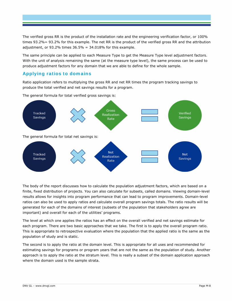
DNV GL – www.dnvgl.com Page M-8
The verified gross RR is the product of the installation rate and the engineering verification factor, or 100% times 93.2%= 93.2% for this example. The net RR is the product of the verified gross RR and the attribution adjustment, or 93.2% times 36.5% = 34.018% for this example.
The same principle can be applied to each Measure Type to get the Measure Type level adjustment factors. With the unit of analysis remaining the same (at the measure type level), the same process can be used to produce adjustment factors for any domain that we are able to define for the whole sample.
Applying ratios to domains
Ratio application refers to multiplying the gross RR and net RR times the program tracking savings to produce the total verified and net savings results for a program.
The general formula for total verified gross savings is:
The general formula for total net savings is:
The body of the report discusses how to calculate the population adjustment factors, which are based on a finite, fixed distribution of projects. You can also calculate for subsets, called domains. Viewing domain-level results allows for insights into program performance that can lead to program improvements. Domain-level ratios can also be used to apply ratios and calculate overall program savings totals. The ratio results will be generated for each of the domains of interest (subsets of the population that stakeholders agree are important) and overall for each of the utilities’ programs.
The level at which one applies the ratios has an effect on the overall verified and net savings estimate for each program. There are two basic approaches that we take. The first is to apply the overall program ratio. This is appropriate to retrospective evaluation where the population that the applied ratio is the same as the population of study and is static.
The second is to apply the ratio at the domain level. This is appropriate for all uses and recommended for estimating savings for programs or program years that are not the same as the population of study. Another approach is to apply the ratio at the stratum level. This is really a subset of the domain application approach where the domain used is the sample strata.

DNV GL – www.dnvgl.com Page M-9
We recommend applying ratios by domains in most cases in order to improve accuracy. Assuming a sufficient sample size in each domain, domain-level precisions are usually sufficient for the approach. While 90/10 relative precision is typically the threshold targeted for an overall result, precisions usually have lower threshold for domain-level application as the resulting precision of the overall result will be better than the component parts.
If one domain has an extreme adjustment, the accuracy of the overall result is improved if domain level ratios are applied to the domain level savings. Table 8-93 shows an example where we apply the gross RR and net RR directly and by domains. The sample weighted savings in the example closely match the population savings: one domain, process heat, is 3.2% different, while the other domains are each within 3% and overall the difference is less than 1%. The ratios and resulting savings are also similar, within one% of one another. Though the results in the example are similar, the final net savings are more accurate when calculated by domains. In the example, both space heat and maintenance measures had very different attributions from process heat and each were slightly over-represented in the weighted sample savings, which resulted in lower net savings when we applied the overall ratio directly.
Table 8-93: Example of ratios applied overall vs. by domains
Measure Type
A B C D
Verified Gross
Savings (A*C)
Net Savings (A*D)
Population m3
Sample Weighted
m3 Gross
RR Net RR Space Heat 1,950,000 1,972,000 99.6% 19.3% 1,943,078 375,761 Process Heat 1,090,000 1,055,000 83.7% 75.8% 912,810 826,024 Maintenance 585,000 600,000 88.7% 9.3% 518,700 54,600 Overall - Ratios Applied Directly 3,625,000 3,627,000 93.2% 34.1% 3,378,636 1,234,819
Overall - Ratios Applied by Domains and Summed
3,625,000 93.1% 34.7% 3,374,589 1,256,384
Difference 0.1% -0.6% 4,047 -21,566
Neither applying the overall ratio directly nor by domains has an inherent systemic bias, but when the differences among the domain ratios are significant, applying by domains results in improved accuracy.
The choice between how to apply the ratios does not affect whether or which domains are reported. There is a large inherent value in looking at program results by multiple domains in order to better understand where the program is doing well and what areas have room for improvement.
Criteria for selecting domains for reporting and application DNV GL will select the domains that are reported and those that will be applied to estimate gross and net savings for the programs.
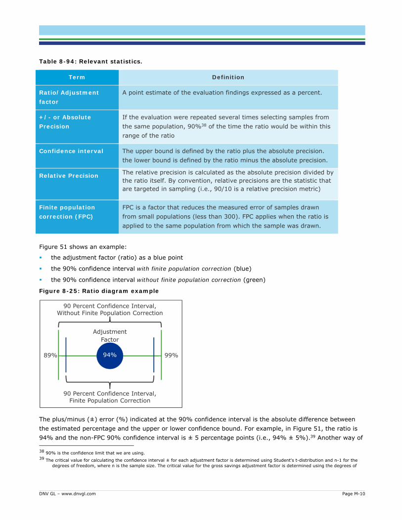
DNV GL – www.dnvgl.com Page M-10
Table 8-94: Relevant statistics.
Term Definition
Ratio/Adjustment factor
A point estimate of the evaluation findings expressed as a percent.
+/- or Absolute Precision
If the evaluation were repeated several times selecting samples from the same population, 90%38 of the time the ratio would be within this range of the ratio
Confidence interval The upper bound is defined by the ratio plus the absolute precision. the lower bound is defined by the ratio minus the absolute precision.
Relative Precision The relative precision is calculated as the absolute precision divided by the ratio itself. By convention, relative precisions are the statistic that are targeted in sampling (i.e., 90/10 is a relative precision metric)
Finite population correction (FPC)
FPC is a factor that reduces the measured error of samples drawn from small populations (less than 300). FPC applies when the ratio is applied to the same population from which the sample was drawn.
Figure 51 shows an example:
the adjustment factor (ratio) as a blue point
the 90% confidence interval with finite population correction (blue)
the 90% confidence interval without finite population correction (green)
Figure 8-25: Ratio diagram example
The plus/minus (±) error (%) indicated at the 90% confidence interval is the absolute difference between the estimated percentage and the upper or lower confidence bound. For example, in Figure 51, the ratio is 94% and the non-FPC 90% confidence interval is ± 5 percentage points (i.e., 94% ± 5%).39 Another way of 38 90% is the confidence limit that we are using. 39 The critical value for calculating the confidence interval ± for each adjustment factor is determined using Student's t-distribution and n-1 for the
degrees of freedom, where n is the sample size. The critical value for the gross savings adjustment factor is determined using the degrees of
Adjustment Factor
90 Percent Confidence Interval, Without Finite Population Correction
90 Percent Confidence Interval, Finite Population Correction
89% 99%94%

DNV GL – www.dnvgl.com Page M-11
saying this is that there is a 90% probability that the actual ratio for the next year’s program lies between 89 and 99%. Figure 8-26 demonstrates this concept by showing twenty hypothetical confidence intervals calculated from twenty different samples of the same population. Eighteen out of twenty (90%) include the true population ratio
Figure 8-26. Ninety Percent Confidence Interval
Note: Each horizontal line represents a confidence interval. Yellow confidence intervals do not include the actual ratio.
The relative precision of the ratio is calculated as 5%/94% =5.3%.
For low ratios, relative precisions may be quite high, even when the confidence interval around the ratio is quite narrow. Consider a ratio of 40% with the same 5% absolute precision as in the above example. While the absolute precisions are the same, the latter ratio (40%) has a relative precision of 5%/40% =12.5%.
Because relative precisions can over-represent error for low ratios (and under-represent errors for ratios above 100%), we prefer to set thresholds for reporting and application based on the absolute precision rather than the relative precision.
For determining which ratios to report and apply we will use the following rules:
The minimum sample size for a reporting or application domain will be five.
The absolute precision threshold for reporting ratio for a domain will be +/- 20% at 90% confidence with FPC-on.
The absolute precision threshold for applying ratio for a domain will be +/- 15% at 90% confidence with FPC-on for retrospective application.
The absolute precision threshold for applying ratio for a domain will be +/- 20% at 90% confidence with FPC-off for prospective application.
freedom based on the minimum sample size for the components of the adjustment factor. The gross savings adjustment factor is a product of the installation rate and the engineering verification factor. For 2-tailed estimates (ratios that could be above or below 100%) the appropriate t-stat used to calculate precision from the standard error is close to 1.645.
Actual Installation
Rate

DNV GL – www.dnvgl.com Page M-12
Reporting domains will be defined as combinations of the following categorizations where sample sizes and precisions allow:
Stratification segments
NTG Category (for FR and SO)
CPSV Category (for Gross results)
Measure types (shown in later tables)
Table 8-95 and Table 8-97 present the maximum number of reporting domains for the NTG results and Table 8-98 and Table 8-99 present the maximum number of reporting domains for the CPSV results.
There will be cases where some of the groups defined by a categorization have sufficient precision, while others do not. In these cases, we will combine the groups that do not meet reporting thresholds into an “other” group. For example, we may have sufficient precision to report separate ratios for Enbridge Commercial Controls, Heat Recovery and HVAC, but not enough to report the ratios for the other six measure types. In this case, we will report the three groups that we have sufficient precision for and group the rest into a “Balance of commercial/Other” group. Table 8-96 provides an example of how the Enbridge NTG domains presented in Table 8-95 could potentially be collapsed during ratio estimation.
No results will be reported that blend Union and Enbridge samples. Large Volume and RunitRight will also not be combined with other programs segments due to their different designs.
For application of CPSV results our initial list of application domains will be within stratification segment with separate domains for each CPSV category and measure type (as shown in the tables below). Those domains that meet the pre-defined precision and sample size criteria, described above, will have results applied at this level. For the rest of the list we will combine domains in the most logical manner appropriate to the ratio in order to achieve combinations that meet criteria and where possible are a meaningful grouping of measures. For example, we will combine CPSV categories within measure types and combine measure types within CPSV categories as is most reasonable given the estimation approaches used (i.e. if there is little difference in simple vs complex measures in the calculation method for building shell measures we would combine the simple and complex building shell first rather than simple building shell into a “simple-other” domain).
For application of NTG results the same process will be used as for CPSV, but with the NTG category substituting for the CPSV category.

DNV GL – www.dnvgl.com Page M-13
Table 8-95. Enbridge NTG domains
Utility Program NTG Category Measure Type Enbridge Commercial Action Operational Improvements Enbridge Commercial Equipment Building Shell Enbridge Commercial Equipment Controls Enbridge Commercial Equipment HVAC Enbridge Commercial Equipment Heat Recovery Enbridge Commercial Equipment Steam and Hot Water Enbridge Industrial Action Operational Improvements Enbridge Industrial Equipment Building Shell Enbridge Industrial Equipment Controls Enbridge Industrial Equipment Greenhouse Enbridge Industrial Equipment HVAC Enbridge Industrial Equipment Heat Recovery Enbridge Industrial Equipment Other Equipment Enbridge Industrial Equipment Process Heat Enbridge Industrial Equipment Steam and Hot Water Enbridge Multi-Residential All Controls Enbridge Multi-Residential All HVAC Enbridge Multi-Residential All Heat Recovery Enbridge Multi-Residential All Operational Improvements Enbridge Multi-Residential All Steam and Hot Water Enbridge RunitRight Action RunitRight
Table 8-96. Example of potential Enbridge NTG domain collapsing
Utility Program NTG Category Measure Type Enbridge Commercial & Multi-Residential Equipment Controls Enbridge Commercial & Multi-Residential Equipment HVAC Enbridge Commercial & Multi-Residential Equipment Steam and Hot Water Enbridge Commercial Equipment Other Commercial Equipment Enbridge Industrial Action Operational Improvements Enbridge Industrial Equipment Controls Enbridge Industrial Equipment Heat Recovery Enbridge Industrial Equipment Other Industrial Equipment Enbridge Multi-Residential All Multi-Residential Other Enbridge RunitRight Action RunitRight

DNV GL – www.dnvgl.com Page M-14
Table 8-97. Union NTG domains
Utility Program NTG Category Measure Type Union Commercial Action Controls Union Commercial Action Maintenance Union Commercial Action Optimization Union Commercial Action Steam and Hot Water Union Commercial Equipment Building Shell Union Commercial Equipment Controls Union Commercial Equipment HVAC Union Commercial Equipment Heat Recovery Union Commercial Equipment New Construction Union Commercial Equipment Other Equipment Union Commercial Equipment Steam and Hot Water Union Industrial Action Controls Union Industrial Action HVAC Union Industrial Action Maintenance Union Industrial Action Optimization Union Industrial Action Steam and Hot Water Union Industrial Equipment Ag and Greenhouse Union Industrial Equipment Building Shell Union Industrial Equipment Controls Union Industrial Equipment HVAC Union Industrial Equipment Heat Recovery Union Industrial Equipment Other Equipment Union Industrial Equipment Process Heat Union Industrial Equipment Steam and Hot Water Union Large Volume Action HVAC Union Large Volume Action Heat Recovery Union Large Volume Action Maintenance Union Large Volume Action Optimization Union Large Volume Action Other Equipment Union Large Volume Equipment Ag and Greenhouse Union Large Volume Equipment Building Shell Union Large Volume Equipment Controls Union Large Volume Equipment HVAC Union Large Volume Equipment Heat Recovery Union Large Volume Equipment New Construction Union Large Volume Equipment Other Equipment Union Large Volume Equipment Steam and Hot Water Union Multi-Family All Controls Union Multi-Family All New Construction Union Multi-Family All Steam and Hot Water

DNV GL – www.dnvgl.com Page M-15
Table 8-98. Enbridge CPSV domains
Utility Program CPSV Category Measure Type Enbridge Commercial Complex Building Shell Enbridge Commercial Complex Controls Enbridge Commercial Complex HVAC Enbridge Commercial Complex Heat Recovery Enbridge Commercial Complex Operational Improvements Enbridge Commercial Complex Steam and Hot Water
Enbridge Commercial Simple Building Shell Enbridge Commercial Simple Controls Enbridge Commercial Simple HVAC Enbridge Commercial Simple Heat Recovery Enbridge Commercial Simple Operational Improvements Enbridge Commercial Simple Steam and Hot Water
Enbridge Industrial Complex Building Shell Enbridge Industrial Complex Controls Enbridge Industrial Complex Greenhouse Enbridge Industrial Complex HVAC Enbridge Industrial Complex Heat Recovery Enbridge Industrial Complex Operational Improvements Enbridge Industrial Complex Other Equipment Enbridge Industrial Complex Steam and Hot Water
Enbridge Industrial Simple Building Shell Enbridge Industrial Simple Greenhouse Enbridge Industrial Simple HVAC Enbridge Industrial Simple Heat Recovery Enbridge Industrial Simple Operational Improvements Enbridge Industrial Simple Other Equipment Enbridge Industrial Simple Process Heat Enbridge Industrial Simple Steam and Hot Water
Enbridge Multi‐Residential Complex Controls Enbridge Multi‐Residential Complex HVAC Enbridge Multi‐Residential Complex Heat Recovery Enbridge Multi‐Residential Complex Steam and Hot Water
Enbridge Multi‐Residential Simple Controls Enbridge Multi‐Residential Simple HVAC Enbridge Multi‐Residential Simple Heat Recovery Enbridge Multi‐Residential Simple Operational Improvements Enbridge Multi‐Residential Simple Steam and Hot Water

DNV GL – www.dnvgl.com Page M-16
Table 8-99. Union CPSV domains
Utility Program CPSV Category Measure Type Union Commercial Complex Building Shell Union Commercial Complex Controls Union Commercial Complex HVAC Union Commercial Complex Heat Recovery Union Commercial Complex Maintenance Union Commercial Complex New Construction Union Commercial Complex Optimization Union Commercial Complex Other Equipment Union Commercial Complex Steam and Hot Water Union Commercial Simple Building Shell Union Commercial Simple Controls Union Commercial Simple HVAC Union Commercial Simple Heat Recovery Union Commercial Simple Maintenance Union Commercial Simple Optimization Union Commercial Simple Other Equipment Union Commercial Simple Steam and Hot Water Union Industrial Complex Ag and Greenhouse Union Industrial Complex Building Shell Union Industrial Complex Controls Union Industrial Complex HVAC Union Industrial Complex Heat Recovery Union Industrial Complex Maintenance Union Industrial Complex Optimization Union Industrial Complex Other Equipment Union Industrial Complex Process Heat Union Industrial Complex Steam and Hot Water Union Industrial Simple Ag and Greenhouse Union Industrial Simple Building Shell Union Industrial Simple Controls Union Industrial Simple HVAC Union Industrial Simple Heat Recovery Union Industrial Simple Maintenance Union Industrial Simple Optimization Union Industrial Simple Process Heat Union Industrial Simple Steam and Hot Water Union Large Volume Complex Ag and Greenhouse Union Large Volume Complex Building Shell Union Large Volume Complex Controls Union Large Volume Complex HVAC Union Large Volume Complex Heat Recovery Union Large Volume Complex Maintenance Union Large Volume Complex New Construction Union Large Volume Complex Optimization Union Large Volume Complex Other Equipment Union Large Volume Complex Steam and Hot Water Union Multi-family Complex Controls Union Multi-family Complex Heat Recovery Union Multi-family Complex New Construction Union Multi-family Complex Other Equipment Union Multi-family Simple Building Shell Union Multi-family Simple Controls Union Multi-family Simple HVAC Union Multi-family Simple Steam and Hot Water

DNV GL – www.dnvgl.com Page N-1
APPENDIX N. DATA COLLECTION INSTRUMENTS The embedded documents below are the interview guides used for participant and vendor data collection for the NTG portion of the evaluation.
Participant IDI
Vendor IDI

DNV GL – www.dnvgl.com Page O-1
APPENDIX O. FREE-RIDERSHIP SURVEY DATA QUALITY CONTROL This appendix includes summaries of survey questions used to QC the attribution results. The QC process involves comparison of scored question responses to question responses in the same interview. Interviews with potentially conflicting responses are reviewed by the PM, who reads the entire interview before determining if an adjustment to a score is required. In total, 29 measure free ridership scores were adjusted through this process and five measures were dropped. Table 8-100 provides the count of measures adjusted for each utility and whether the adjustment increased (Inc) or decreased (Dec) attribution for that measure.
Table 8-100. PM Quality Assurance Adjustments.
PM Quality Assurance Status
Union Enbridge Overall
Inc Dec Total Inc Dec Total Inc Dec Total Total Measures Completed from FR IDIs 281 177 458
Not Adjusted 260 164 424
PM A
djus
tmen
ts f
rom
QA
Dropped 4 1 5
Assign DNK Attribution, but unclear amount.
Timing 1 0 1 0 0 0 1 0 1
Efficiency 3 0 3 7 0 7 10 0 10
Quantity/Size 2 0 2 1 0 1 3 0 3
Adjust Score Attribution Clear based on open, conflicted with scored response
Timing 1 0 1 1 1 2 2 1 3
Efficiency 3 1 4 1 0 1 3 2 5
Quantity/Size 0 1 1 0 0 0 1 1
Gross Baseline Efficiency Adjustment 3 2 5 0 1 1 3 3 6
The attribution results used to create the following tables also include the vendor component of attribution. Consequently, the attribution bin may be higher than reported by the customer alone. This section includes the following tables:
PF8 responses by overall attribution bin
PF9 responses by overall attribution bin.
Dat0 responses versus overall attribution bin
Dat6 responses versus overall attribution bin
Dat6 responses versus overall spa bin

DNV GL – www.dnvgl.com Page O-2
Union Commercial and Industrial Programs Table 8-101. PF8 and Attribution Bin, Union Custom C&I programs*
PF8. For the project, did you become aware of utility program incentives and services…? Attribution Bin PF8 Customers Units of
Analysis Measures Percent Savings
Full
Before starting the project 16 31 43 18% As soon as you began exploring equipment options * * * <1%
While exploring equipment options, but before making equipment decision * * * 5%
After making an equipment decision 0 0 0 0% After installing the equipment * * * <1% Don't Know/ Refused 0 0 0 0%
Partial
Before starting the project 26 46 64 23% As soon as you began exploring equipment options 6 7 10 4%
While exploring equipment options, but before making equipment decision * * * <1%
After making an equipment decision 0 0 0 0% After installing the equipment 0 0 0 0% Don't Know/ Refused * * 7 9%
None
Before starting the project 26 35 45 27% As soon as you began exploring equipment options * * 5 5%
While exploring equipment options, but before making equipment decision * * * 2%
After making an equipment decision 5 6 6 3% After installing the equipment * 5 5 4% Don't Know/ Refused * * * <1%
For confidentiality reasons the numbers of customers, units of analysis and measures less than 5 are not displayed. *Attribution includes both a customer and a vendor component when the customer indicated that the vendor was influential in their decision.
Consequently, the attribution bin may be higher for a measure than indicated by the customer.

DNV GL – www.dnvgl.com Page O-3
Table 8-102. PF9 and Attribution Bin, Union Custom C&I programs*
PF9. When did the utility first get involved in this project? Was it… Attribution Bin PF9 Customers Units of
Analysis Measures Percent Savings
Full
Before starting the project 12 24 31 15% As soon as you began exploring equipment options * 7 13 3%
While exploring equipment options, but before making equipment decision * * * 5%
After making an equipment decision * * * <1% After installing the equipment * * * <1% Don't Know/ Refused 0 0 0 0%
Partial
Before starting the project 16 30 42 16% As soon as you began exploring equipment options 12 20 32 12%
While exploring equipment options, but before making equipment decision 5 5 5 8%
After making an equipment decision 0 0 0 0% After installing the equipment 0 0 0 0% Don't Know/ Refused * * * 1%
None
Before starting the project 13 19 25 20% As soon as you began exploring equipment options 7 8 11 5%
While exploring equipment options, but before making equipment decision * 5 5 2%
After making an equipment decision 8 9 9 5% After installing the equipment * 7 9 7% Don't Know/ Refused 6 6 6 <1%
For confidentiality reasons the numbers of customers, units of analysis and measures less than 5 are not displayed. *Attribution includes both a customer and a vendor component when the customer indicated that the vendor was influential in their decision.
Consequently, the attribution bin may be higher for a measure than indicated by the customer.

DNV GL – www.dnvgl.com Page O-4
Table 8-103. Dat0 and Attribution Bin, Union Custom C&I programs*
DAT0. Without the program, would you say the likelihood of [installing / performing] the project was...? Attribution Bin Dat0 Customers Units of
Analysis Measures Percent Savings
Full
Very likely * * 6 2% Somewhat likely * * 5 3% Not very likely 6 7 8 3% Very unlikely 10 21 30 14% Don't Know/ Refused 0 0 0 0%
Partial
Very likely 12 13 15 11% Somewhat likely 17 19 25 13% Not very likely 7 20 34 11% Very unlikely * * * 1% Don't Know/ Refused * * 6 1%
None
Very likely 33 41 46 30% Somewhat likely 9 10 16 11% Not very likely * * * <1% Very unlikely 0 0 0 0% Don't Know/ Refused * * * <1%
For confidentiality reasons the numbers of customers, units of analysis and measures less than 5 are not displayed. *Attribution includes both a customer and a vendor component when the customer indicated that the vendor was influential in their decision.
Consequently, the attribution bin may be higher for a measure than indicated by the customer.

DNV GL – www.dnvgl.com Page O-5
Table 8-104. Dat6 and Attribution Bin, Union Custom C&I programs*
Dat6. Without any utility assistance for this or any other projects in the past, what is the percent likelihood that you would have done this project? (0% means no chance and 100% means definitely completed without assistance) Attribution Bin Dat6 Customers Units of
Analysis Measures Percent Savings
Full
0% 8 18 25 15% 1% to 25% 6 8 12 <1% 26% to 50% * * * 2% 51% to 75% * * * 2% 76% to 99% 0 0 0 0% 100% * * 5 3% Don't Know/ Refused * * * <1%
Partial
0% * * * <1% 1% to 25% * * * <1% 26% to 50% * * * 3% 51% to 75% * * * 3% 76% to 99% * * 7 3% 100% 31 41 49 32% Don't Know/ Refused * * * <1%
None
0% * * * <1% 1% to 25% 9 12 26 12% 26% to 50% 6 19 21 9% 51% to 75% * * 8 2% 76% to 99% 6 6 6 3% 100% 11 15 19 11% Don't Know/ Refused * * * <1%
For confidentiality reasons the numbers of customers, units of analysis and measures less than 5 are not displayed. *Attribution includes both a customer and a vendor component when the customer indicated that the vendor was influential in their decision.
Consequently, the attribution bin may be higher for a measure than indicated by the customer.

DNV GL – www.dnvgl.com Page O-6
Table 8-105. Dat6 and SPA Bin, Union Custom C&I programs
Dat6. Without any utility assistance for this or any other projects in the past, what is the percent likelihood that you would have done this project? (0% means no chance and 100% means definitely completed without assistance)
SPA Bin Dat6 Customers Units of Analysis Measures Percent
Savings
Full
0% 8 18 25 15% 1% to 25% 6 8 12 <1% 26% to 50% * * * 2% 51% to 75% * * * 2% 76% to 99% 0 0 0 0% 100% * * 5 3% Don't Know/ Refused * * * <1%
Partial
0% * * * <1% 1% to 25% 7 8 15 5% 26% to 50% * * * 3% 51% to 75% * 5 5 3% 76% to 99% 6 6 9 3% 100% 38 53 63 40% Don't Know/ Refused * * * <1%
None
0% 0 0 0 0% 1% to 25% 5 5 12 7% 26% to 50% 6 19 21 9% 51% to 75% * * 7 2% 76% to 99% * * * 3% 100% * * 5 3% Don't Know/ Refused 0 0 0 0%

DNV GL – www.dnvgl.com Page O-7
Union Large Volume Table 8-106. PF8 and Attribution Bin, Union Large Volume*
PF8. For the project, did you become aware of utility program incentives and services…? Attribution Bin PF8 Customers Units of
Analysis Measures Percent Savings
Full
Before starting the project * * * <1% As soon as you began exploring equipment options * * * <1%
While exploring equipment options, but before making equipment decision 0 0 0 0%
After making an equipment decision 0 0 0 0% After installing the equipment 0 0 0 0% Don't Know/ Refused 0 0 0 0%
Partial
Before starting the project 9 16 28 24% As soon as you began exploring equipment options 0 0 0 0%
While exploring equipment options, but before making equipment decision 0 0 0 0%
After making an equipment decision 0 0 0 0% After installing the equipment 0 0 0 0% Don't Know/ Refused 0 0 0 0%
None
Before starting the project 12 21 37 64% As soon as you began exploring equipment options * * * <1%
While exploring equipment options, but before making equipment decision 0 0 0 0%
After making an equipment decision * * * <1% After installing the equipment * 6 9 9% Don't Know/ Refused * * 5 2%
For confidentiality reasons the numbers of customers, units of analysis and measures less than 5 are not displayed. *Attribution includes both a customer and a vendor component when the customer indicated that the vendor was influential in their decision.
Consequently, the attribution bin may be higher for a measure than indicated by the customer.

DNV GL – www.dnvgl.com Page O-8
Table 8-107. PF9 and Attribution Bin, Union Large Volume*
PF9. When did the utility first get involved in this project? Was it… Attribution Bin PF9 Customers Units of
Analysis Measures Percent Savings
Full
Before starting the project * * * <1% As soon as you began exploring equipment options 0 0 0 0%
While exploring equipment options, but before making equipment decision * * * <1%
After making an equipment decision 0 0 0 0% After installing the equipment 0 0 0 0% Don't Know/ Refused 0 0 0 0%
Partial
Before starting the project 6 12 24 21% As soon as you began exploring equipment options * * * 2%
While exploring equipment options, but before making equipment decision * * * 1%
After making an equipment decision 0 0 0 0% After installing the equipment 0 0 0 0% Don't Know/ Refused 0 0 0 0%
None
Before starting the project 6 14 21 46% As soon as you began exploring equipment options 7 7 10 8%
While exploring equipment options, but before making equipment decision * * * 2%
After making an equipment decision * * 8 9% After installing the equipment * 6 9 9% Don't Know/ Refused * * * 1%
For confidentiality reasons the numbers of customers, units of analysis and measures less than 5 are not displayed. *Attribution includes both a customer and a vendor component when the customer indicated that the vendor was influential in their decision.
Consequently, the attribution bin may be higher for a measure than indicated by the customer.
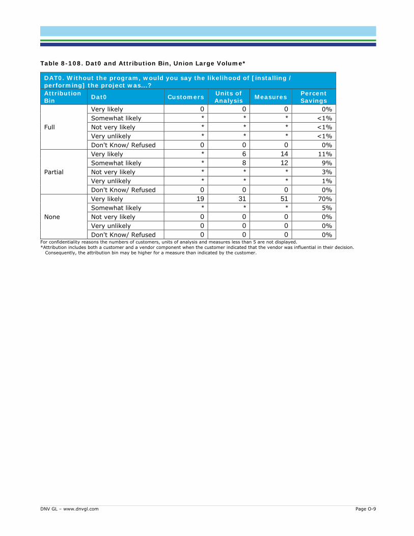
DNV GL – www.dnvgl.com Page O-9
Table 8-108. Dat0 and Attribution Bin, Union Large Volume*
DAT0. Without the program, would you say the likelihood of [installing / performing] the project was...? Attribution Bin Dat0 Customers Units of
Analysis Measures Percent Savings
Full
Very likely 0 0 0 0% Somewhat likely * * * <1% Not very likely * * * <1% Very unlikely * * * <1% Don't Know/ Refused 0 0 0 0%
Partial
Very likely * 6 14 11% Somewhat likely * 8 12 9% Not very likely * * * 3% Very unlikely * * * 1% Don't Know/ Refused 0 0 0 0%
None
Very likely 19 31 51 70% Somewhat likely * * * 5% Not very likely 0 0 0 0% Very unlikely 0 0 0 0% Don't Know/ Refused 0 0 0 0%
For confidentiality reasons the numbers of customers, units of analysis and measures less than 5 are not displayed. *Attribution includes both a customer and a vendor component when the customer indicated that the vendor was influential in their decision.
Consequently, the attribution bin may be higher for a measure than indicated by the customer.

DNV GL – www.dnvgl.com Page O-10
Table 8-109. Dat6 and Attribution Bin, Union Large Volume*
Dat6. Without any utility assistance for this or any other projects in the past, what is the percent likelihood that you would have done this project? (0% means no chance and 100% means definitely completed without assistance) Attribution Bin Dat6 Customers Units of
Analysis Measures Percent Savings
Full
0% 0 0 0 0% 1% to 25% * * * <1% 26% to 50% * * * <1% 51% to 75% 0 0 0 0% 76% to 99% 0 0 0 0% 100% * * * <1% Don't Know/ Refused 0 0 0 0%
Partial
0% 0 0 0 0% 1% to 25% * * * 3% 26% to 50% 0 0 0 0% 51% to 75% 0 0 0 0% 76% to 99% * * 6 7% 100% 16 29 46 64% Don't Know/ Refused 0 0 0 0%
None
0% 0 0 0 0% 1% to 25% 0 0 0 0% 26% to 50% * * * <1% 51% to 75% * * * 4% 76% to 99% * * * 3% 100% 6 9 19 17% Don't Know/ Refused 0 0 0 0%
For confidentiality reasons the numbers of customers, units of analysis and measures less than 5 are not displayed. *Attribution includes both a customer and a vendor component when the customer indicated that the vendor was influential in their decision.
Consequently, the attribution bin may be higher for a measure than indicated by the customer.

DNV GL – www.dnvgl.com Page O-11
Table 8-110. Dat6 and SPA Bin, Union Large Volume*
Dat6. Without any utility assistance for this or any other projects in the past, what is the percent likelihood that you would have done this project? (0% means no chance and 100% means definitely completed without assistance)
SPA Bin Dat6 Customers Units of Analysis Measures Percent
Savings
Full
0% 0 0 0 0% 1% to 25% * * * <1% 26% to 50% * * * <1% 51% to 75% 0 0 0 0% 76% to 99% 0 0 0 0% 100% * * * <1% Don't Know/ Refused 0 0 0 0%
Partial
0% 0 0 0 0% 1% to 25% * * * 3% 26% to 50% 0 0 0 0% 51% to 75% * * * 4% 76% to 99% * 5 7 9% 100% 18 34 54 69% Don't Know/ Refused 0 0 0 0%
None
0% 0 0 0 0% 1% to 25% 0 0 0 0% 26% to 50% * * * <1% 51% to 75% 0 0 0 0% 76% to 99% * * * <1% 100% * * 11 13% Don't Know/ Refused 0 0 0 0%

DNV GL – www.dnvgl.com Page O-12
Enbridge Commercial and Industrial Programs Table 8-111. PF8 and Attribution Bin, Enbridge Custom C&I programs*
PF8. For the project, did you become aware of utility program incentives and services…? Attribution Bin PF8 Customers Units of
Analysis Measures Percent Savings
Full
Before starting the project 11 16 22 12% As soon as you began exploring equipment options * * * <1%
While exploring equipment options, but before making equipment decision * * * <1%
After making an equipment decision 0 0 0 0% After installing the equipment 0 0 0 0% Don't Know/ Refused * * * 4%
Partial
Before starting the project 33 47 60 31% As soon as you began exploring equipment options 8 9 11 14%
While exploring equipment options, but before making equipment decision * * * <1%
After making an equipment decision 0 0 0 0% After installing the equipment 0 0 0 0% Don't Know/ Refused * * * 1%
None
Before starting the project 31 42 47 28% As soon as you began exploring equipment options 6 7 8 3%
While exploring equipment options, but before making equipment decision 0 0 0 0%
After making an equipment decision * * * 2% After installing the equipment 0 0 0 0% Don't Know/ Refused * * * 3%
For confidentiality reasons the numbers of customers, units of analysis and measures less than 5 are not displayed. *Attribution includes both a customer and a vendor component when the customer indicated that the vendor was influential in their decision.
Consequently, the attribution bin may be higher for a measure than indicated by the customer.
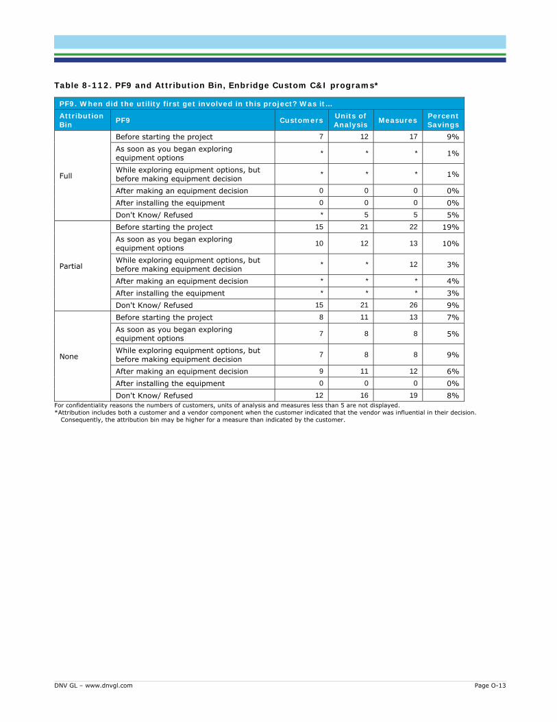
DNV GL – www.dnvgl.com Page O-13
Table 8-112. PF9 and Attribution Bin, Enbridge Custom C&I programs*
PF9. When did the utility first get involved in this project? Was it… Attribution Bin PF9 Customers Units of
Analysis Measures Percent Savings
Full
Before starting the project 7 12 17 9% As soon as you began exploring equipment options * * * 1%
While exploring equipment options, but before making equipment decision * * * 1%
After making an equipment decision 0 0 0 0% After installing the equipment 0 0 0 0% Don't Know/ Refused * 5 5 5%
Partial
Before starting the project 15 21 22 19% As soon as you began exploring equipment options 10 12 13 10%
While exploring equipment options, but before making equipment decision * * 12 3%
After making an equipment decision * * * 4% After installing the equipment * * * 3% Don't Know/ Refused 15 21 26 9%
None
Before starting the project 8 11 13 7% As soon as you began exploring equipment options 7 8 8 5%
While exploring equipment options, but before making equipment decision 7 8 8 9%
After making an equipment decision 9 11 12 6% After installing the equipment 0 0 0 0% Don't Know/ Refused 12 16 19 8%
For confidentiality reasons the numbers of customers, units of analysis and measures less than 5 are not displayed. *Attribution includes both a customer and a vendor component when the customer indicated that the vendor was influential in their decision.
Consequently, the attribution bin may be higher for a measure than indicated by the customer.

DNV GL – www.dnvgl.com Page O-14
Table 8-113. Dat0 and Attribution Bin, Enbridge Custom C&I programs*
DAT0. Without the program, would you say the likelihood of [installing / performing] the project was...? Attribution Bin Dat0 Customers Units of
Analysis Measures Percent Savings
Full
Very likely * * * <1% Somewhat likely * * * 3% Not very likely 7 12 15 9% Very unlikely 6 6 6 5% Don't Know/ Refused 0 0 0 0%
Partial
Very likely 13 16 17 10% Somewhat likely 19 22 31 27% Not very likely 14 20 25 10% Very unlikely * * * <1% Don't Know/ Refused * * * <1%
None
Very likely 33 40 46 28% Somewhat likely 10 14 14 8% Not very likely 0 0 0 0% Very unlikely 0 0 0 0% Don't Know/ Refused 0 0 0 0%
For confidentiality reasons the numbers of customers, units of analysis and measures less than 5 are not displayed. *Attribution includes both a customer and a vendor component when the customer indicated that the vendor was influential in their decision.
Consequently, the attribution bin may be higher for a measure than indicated by the customer.

DNV GL – www.dnvgl.com Page O-15
Table 8-114. Dat6 and Attribution Bin, Enbridge Custom C&I programs*
Dat6. Without any utility assistance for this or any other projects in the past, what is the percent likelihood that you would have done this project? (0% means no chance and 100% means definitely completed without assistance) Attribution Bin Dat6 Customers Units of
Analysis Measures Percent Savings
Full
0% 5 10 12 9% 1% to 25% * * * 2% 26% to 50% * * 7 5% 51% to 75% 0 0 0 0% 76% to 99% 0 0 0 0% 100% * * * 1% Don't Know/ Refused 0 0 0 0%
Partial
0% 0 0 0 0% 1% to 25% 0 0 0 0% 26% to 50% * * * <1% 51% to 75% * * * 3% 76% to 99% 5 7 7 3% 100% 31 37 41 29% Don't Know/ Refused * 5 7 <1%
None
0% * * * <1% 1% to 25% * 5 5 2% 26% to 50% 12 18 23 12% 51% to 75% 5 7 7 5% 76% to 99% 9 10 18 6% 100% 13 16 18 18% Don't Know/ Refused * * * 3%
For confidentiality reasons the numbers of customers, units of analysis and measures less than 5 are not displayed. *Attribution includes both a customer and a vendor component when the customer indicated that the vendor was influential in their decision.
Consequently, the attribution bin may be higher for a measure than indicated by the customer.

DNV GL – www.dnvgl.com Page O-16
Table 8-115. Dat6 and SPA Bin, Enbridge Custom C&I programs*
Dat6. Without any utility assistance for this or any other projects in the past, what is the percent likelihood that you would have done this project? (0% means no chance and 100% means definitely completed without assistance)
SPA Bin Dat6 Customers Units of Analysis Measures Percent
Savings
Full
0% 5 10 12 9% 1% to 25% * * * 2% 26% to 50% * * 7 5% 51% to 75% 0 0 0 0% 76% to 99% 0 0 0 0% 100% * * * 1% Don't Know/ Refused 0 0 0 0%
Partial
0% * * * <1% 1% to 25% * * * 2% 26% to 50% 10 14 19 10% 51% to 75% * 5 5 5% 76% to 99% 8 11 19 6% 100% 39 47 53 42% Don't Know/ Refused * 5 7 <1%
None
0% 0 0 0 0% 1% to 25% * * * <1% 26% to 50% 6 6 6 3% 51% to 75% * 5 5 4% 76% to 99% 5 6 6 3% 100% * 6 6 5% Don't Know/ Refused * * * 3%

DNV GL – www.dnvgl.com Page O-17
RunitRight Table 8-116. PF8 and Attribution Bin, RunItRight*
PF8. For the project, did you become aware of utility program incentives and services…? Attribution Bin PF8 Customers Units of
Analysis Measures Percent Savings
Full
Before starting the project * 6 6 26% As soon as you began exploring equipment options 0 0 0 0%
While exploring equipment options, but before making equipment decision 0 0 0 0%
After making an equipment decision 0 0 0 0% After installing the equipment 0 0 0 0% Don't Know/ Refused 0 0 0 0%
Partial
Before starting the project 5 9 9 66% As soon as you began exploring equipment options 0 0 0 0%
While exploring equipment options, but before making equipment decision 0 0 0 0%
After making an equipment decision 0 0 0 0% After installing the equipment 0 0 0 0% Don't Know/ Refused * * * 9%
None
Before starting the project 0 0 0 0% As soon as you began exploring equipment options 0 0 0 0%
While exploring equipment options, but before making equipment decision 0 0 0 0%
After making an equipment decision 0 0 0 0% After installing the equipment 0 0 0 0% Don't Know/ Refused 0 0 0 0%
For confidentiality reasons the numbers of customers, units of analysis and measures less than 5 are not displayed. *Attribution includes both a customer and a vendor component when the customer indicated that the vendor was influential in their decision.
Consequently, the attribution bin may be higher for a measure than indicated by the customer.

DNV GL – www.dnvgl.com Page O-18
Table 8-117. PF9 and Attribution Bin, RunItRight*
PF9. When did the utility first get involved in this project? Was it… Attribution Bin PF9 Customers Units of
Analysis Measures Percent Savings
Full
Before starting the project * 6 6 26% As soon as you began exploring equipment options 0 0 0 0%
While exploring equipment options, but before making equipment decision 0 0 0 0%
After making an equipment decision 0 0 0 0% After installing the equipment 0 0 0 0% Don't Know/ Refused 0 0 0 0%
Partial
Before starting the project * * * 27% As soon as you began exploring equipment options * * * 19%
While exploring equipment options, but before making equipment decision 0 0 0 0%
After making an equipment decision 0 0 0 0% After installing the equipment 0 0 0 0% Don't Know/ Refused * 5 5 28%
None
Before starting the project 0 0 0 0% As soon as you began exploring equipment options 0 0 0 0%
While exploring equipment options, but before making equipment decision 0 0 0 0%
After making an equipment decision 0 0 0 0% After installing the equipment 0 0 0 0% Don't Know/ Refused 0 0 0 0%
For confidentiality reasons the numbers of customers, units of analysis and measures less than 5 are not displayed. *Attribution includes both a customer and a vendor component when the customer indicated that the vendor was influential in their decision.
Consequently, the attribution bin may be higher for a measure than indicated by the customer.

DNV GL – www.dnvgl.com Page O-19
Table 8-118. Dat0 and Attribution Bin, RunItRight*
DAT0. Without the program, would you say the likelihood of [installing / performing] the project was...?
Attribution Bin Dat0 Customers Units of
Analysis Measures Percent Savings
Full
Very likely 0 0 0 0% Somewhat likely 0 0 0 0% Not very likely * 6 6 26% Very unlikely 0 0 0 0% Don't Know/ Refused 0 0 0 0%
Partial
Very likely * 5 5 48% Somewhat likely * * * 7% Not very likely * * * 19% Very unlikely 0 0 0 0% Don't Know/ Refused 0 0 0 0%
None
Very likely 0 0 0 0% Somewhat likely 0 0 0 0% Not very likely 0 0 0 0% Very unlikely 0 0 0 0% Don't Know/ Refused 0 0 0 0%
For confidentiality reasons the numbers of customers, units of analysis and measures less than 5 are not displayed. *Attribution includes both a customer and a vendor component when the customer indicated that the vendor was influential in their decision.
Consequently, the attribution bin may be higher for a measure than indicated by the customer.

DNV GL – www.dnvgl.com Page O-20
Table 8-119. Dat6 and Attribution Bin, RunItRight*
Dat6. Without any utility assistance for this or any other projects in the past, what is the percent likelihood that you would have done this project? (0% means no chance and 100% means definitely completed without assistance) Attribution Bin Dat6 Customers Units of
Analysis Measures Percent Savings
Full
0% 0 0 0 0% 1% to 25% 0 0 0 0% 26% to 50% * 6 6 26% 51% to 75% 0 0 0 0% 76% to 99% 0 0 0 0% 100% 0 0 0 0% Don't Know/ Refused 0 0 0 0%
Partial
0% 0 0 0 0% 1% to 25% 0 0 0 0% 26% to 50% 0 0 0 0% 51% to 75% 0 0 0 0% 76% to 99% 0 0 0 0% 100% 0 0 0 0% Don't Know/ Refused 0 0 0 0%
None
0% 0 0 0 0% 1% to 25% * * * 7% 26% to 50% * * * 12% 51% to 75% 0 0 0 0% 76% to 99% * * * 7% 100% * 5 5 48% Don't Know/ Refused 0 0 0 0%
For confidentiality reasons the numbers of customers, units of analysis and measures less than 5 are not displayed. *Attribution includes both a customer and a vendor component when the customer indicated that the vendor was influential in their decision.
Consequently, the attribution bin may be higher for a measure than indicated by the customer.

DNV GL – www.dnvgl.com Page O-21
Table 8-120. Dat6 and SPA Bin, RunItRight*
Dat6. Without any utility assistance for this or any other projects in the past, what is the percent likelihood that you would have done this project? (0% means no chance and 100% means definitely completed without assistance)
SPA Bin Dat6 Customers Units of Analysis Measures Percent
Savings
Full
0% 0 0 0 0% 1% to 25% 0 0 0 0% 26% to 50% * 6 6 26% 51% to 75% 0 0 0 0% 76% to 99% 0 0 0 0% 100% 0 0 0 0% Don't Know/ Refused 0 0 0 0%
Partial
0% 0 0 0 0% 1% to 25% 0 0 0 0% 26% to 50% * * * 12% 51% to 75% 0 0 0 0% 76% to 99% * * * 7% 100% * 5 5 48% Don't Know/ Refused 0 0 0 0%
None
0% 0 0 0 0% 1% to 25% * * * 7% 26% to 50% 0 0 0 0% 51% to 75% 0 0 0 0% 76% to 99% 0 0 0 0% 100% 0 0 0 0% Don't Know/ Refused 0 0 0 0%

DNV GL – www.dnvgl.com Page P-1
APPENDIX P. CPSV Details CPSV data collection
Data collection for the TSER sample will be completed via the IDI as described above. Prior to the TSER IDI the interviewing engineer will review project documents and calculations to identify the specific CPSV questions to include in the interview. Following the interview the engineer will complete the TSER verification report, embedded below. Verification reports completed by DNV GL engineers will be reviewed by an Itron engineer and verification reports completed by Itron engineers will be reviewed by a DNV GL engineer.
On-site sample customers will not have engineering questions asked during the IDI. Instead these customers will be asked permission for a follow up site visit. Customers who agree to the site visit will receive a follow up call from Stantec to schedule the visit. Utility staff will be informed of the scheduled visit and invited to attend. Following the on-site visit, the Stantec engineer will complete the on-site verification report, embedded below. An Itron engineer will review the report.
Appendix F has the template forms that each of the data collection approaches will use for the CPSV.
Completed verification reports will be compiled into a draft report to be reviewed by the OEB and EAC. The steps in the CPSV review process are shown in Table 8-121.
Table 8-121: CPSV steps
Step Activity 1 NTG/CPSV Evaluation Team reviews project files provided by utilities
Missing or incomplete documentation will be requested from utilities following review (final opportunity for utilities to provide new information).
2 NTG/CPSV Evaluation Team conducts IDI with customers Collects required CPSV data for TSER sample projects
3 NTG/CPSV Evaluation Team schedules site visits with on-site sample customers, informs utility
4 NTG/CPSV Evaluation Team conducts customer site visit Collects required CPSV data for On-site sample projects
5 NTG/CPSV Evaluation Team drafts project verification reports Contacts utility staff/customer to clarify any site/operational details if needed.
6 EC Team conducts internal review of individual project verification reports Itron reviews projects verified by Stantec and DNV GL
DNV GL reviews projects verified by Itron
7 EC Team shares draft report, including all site verification reports, with OEB for quality control, redacted as necessary.
8 EC Team (OEB team) shares final draft report with EAC, redacted as necessary 9 EAC provides written comments on final draft report 10 EC Team/OEB hold EAC meeting to discuss comments 11 EC Team finalizes report

DNV GL – www.dnvgl.com Page P-2
Gross realization rate
The gross RR is developed through data collected during the CPSV effort, which will verify program-achieved gross savings for measures at a sample of sites. The two components are the installation rate and the engineering verification factor.
The installation rate is derived through the participant survey data collection, which confirms that the reported equipment / measure or something like it was installed at the facility. The resulting analysis value is binary; any similar project to the one reported is considered installed. At the individual measure level, the installation rate is either 100% or 0%.
The engineering verification factor is derived from the data collected during the participant survey data collection for TSER projects and through the on-site visits for other projects. Differences between the reported measure and the “substantially similar” measure installed at the facility are accounted for here. The engineering adjustment factor is the ratio of the evaluator-verified savings to the program-reported savings.
The majority of the CPSV process involves determining the evaluator-verified savings estimate for each measure. The measure-level results are then combined using weights from the sample design to an overall adjustment factor.
To get the evaluation-verified savings for each evaluated measure, the CPSV effort will verify savings based on the applicable standard program baseline and measure life based on the best available information. The formula for estimating measure level verified savings is shown here:
Where:
VGSL – Verified Gross Savings versus standard efficiency equipment on the market (lifetime)
VYL – Verified Estimated Useful Life of the equipment/action
VGSS – Verified Gross Savings versus standard efficiency equipment on the market (annual)
In the Life-Cycle Net Savings (LCNS) method used for this evaluation, the CPSV will also produce a verified savings estimate for accelerated measures using the pre-existing equipment as the baseline (VGSE). Whether or not the measure is accelerated depends on the responses to the attribution survey and will be discussed later. The “versus existing” verified savings will be used in estimating net savings and will not be included in the verified gross savings. The LCNS methodology is further explained in Appendix B.
The CPSV will produce verified values for three required inputs in the Life-Cycle Net Savings (LCNS) attribution:
VGSS – Verified Gross Savings versus standard efficiency equipment on the market
VYL – Verified Estimated Useful Life of the equipment/action
VGSE – Verified Gross Savings versus existing equipment configuration at the time of installation/action: for a sub-set of measures that are accelerated
CPSV site reports will be completed by assigned evaluation engineers and reviewed by an experienced evaluation engineer at another partner firm. Each review will follow the same basic process shown in Figure 8-27.

DNV GL – www.dnvgl.com Page P-3
Figure 8-27: CPSV high-level process
After the initial review and savings calculation, an engineer from a partner firm on the EC team (either DNV GL or Itron) will review the site report, approach, calculation, and verified savings. Following this review the verified savings, verified estimated useful life, reasons for deviation and other pertinent information will be compiled into a single dataset at the unit of analysis level for expansion and integration with the FR analysis.
CPSV rigour levels
The CPSV plan calls for two types of data collection: telephone-supported engineering review (TSER) and on-site. There are adjustments that might entail more or less work at each site. Table 7 details likely engineering effort levels for the standard, increased, and decreased levels. The levels of effort are averages. Some sites may require substantially more effort, while some sites may entail less effort.
Based on the tracking data we have identified the simplest projects as a level of stratification and will used TSER interviews to verify the projects at these sites. The more complex on-site sample will also have varying degrees of effort requirements in order to allow more effort at more complex sites.

DNV GL – www.dnvgl.com Page P-4
Table 8: M&V Description for Proposed Engineering Effort Levels
Effort Level Description
Telephone-supported engineering review (TSER)
Lower rigour projects. Application desk review, telephone interviews, possible revised engineering calculations; primarily for qualitative assessment.
Standard On-site Simpler projects. Detailed application review, on-site verification, collection of data on key parameters, revised engineering calculations, billing data analysis, and possible spot measurements.
Higher Rigour On-site Small, medium and large scale projects that may or may not require monitoring or metering. Detailed application review, on-site verification, collection of data on key parameters, revised engineering calculations, billing data analysis, and possible spot measurements / short term post monitoring.
Very High Rigour On-site
Largest and most complex projects. Detailed application review, on-site verification, collection of data on key parameters, billing/interval data analysis, calibrated simulation models, spot measurements, long-term post monitoring, pre-verification and short-term measurement. May require larger teams, including senior staff and multiple site visits.
Most site-specific impact evaluation efforts for Standard On-site points will fall into the category of lower rigor level of effort. However, there are exceptions and adjustments that might entail more or less work at each site. During the file review adjustments of this sort should be noted and the sites will be reviewed by the engineering team lead (Phani Pagadala) to determine which level of rigour is required. Up to 20 sites (primarily Large Volume) will receive higher rigour on-sites and up to two sites will receive very high rigour on-sites to establish the relative value of increased rigour levels in future evaluation.
Each site will be assigned a single point of contact (POC) for the purposes of communications with the customer, the utility and within CPSV itself. The POC will be a more senior engineering team member who is experienced in the energy efficiency field (preferably a registered professional engineer) and will be responsible for co-ordinating the work of their team, tracking progress on each project review, becoming intimately familiar with the documentation and technical requirements of the work to be performed, ensuring that quality control procedures are implemented, and reporting on project review progress and any issues to the engineering team lead (Phani Pagadala).
Higher rigour sites could involve the addition of elements such as:
A fully specified regression analysis of consumption information from utility bills with inclusion/adjustment for changes and background variables over the time period of the analysis that could potentially be correlated with the gross energy savings being measured.
Twelve (12) months post-retrofit consumption data are required. Twelve (12) months pre-retrofit consumption data are required, unless program design does not allow
pre-retrofit billing data, such as in new construction. In these cases, well-matched control groups and post-retrofit consumption analysis is allowable.

DNV GL – www.dnvgl.com Page P-5
Sampling must be adequate (in general, a minimum of six data points will be required) for a valid regression-based estimate.
Building energy simulation models that are calibrated as described in IPMVP Option D requirements. If appropriate, evaluators may alternatively use an engineering model with calibration.
Retrofit isolation engineering models as described in IPMVP Option B requirements.

DNV GL – www.dnvgl.com Page Q-1
APPENDIX Q. CPSV DISCREPANCY DETAILS This appendix includes additional information about the magnitude of and reasons for gross savings adjustments, by program. Sections are broken up into “Annual savings Adjustments,” which refer to adjustments that do not relate to measure life, and “Measure Life Savings Adjustments” which relate only to measure life but do not affect annual savings. Attempts are made to identify the level of control the program has over each type of adjustment and provide context and opportunities for improvement. Table 8-122 and Table 8-123 show the “Reasons for Discrepancies” which are used throughout this appendix.

DNV GL – www.dnvgl.com Page Q-1
Table 8-122: Descriptions of Annual savings Adjustments
Reason for Discrepancy
Level of Program Control
Description Explanation Recommendation
(where possible, do the following:)
Measured Usage Low
Customer provided metered or measured data that differs from what the program used.
This usually stems from the evaluation having a longer metering period to work with than the ex ante engineering team.
Attempt to use a longer post-installation data collection period if possible.
Efficient Equipment Operating Conditions
Low On-site conditions differed from that claimed by documentation.
These can reflect a change in the operation of the facility since the measure was installed, but also can be due to information that was either not communicated or communicated differently to program engineering staff.
Document any observations or assumptions made with emails, on-site forms, photos, and conversation notes. When evaluators don't have evidence of a value, they have to determine their own value.
Operating Hours Low
Customer reported different operating hours from those reported in ex ante documentation, but no other operational changes.
Change to Calculation Method
Medium Evaluator used a different calculation method.
This stems from the lack of a live calculation tool or the choice to use a different tool (often because the ex ante tool is not able to accommodate all the information obtained on-site).
Maintain and provide live calculation tools with practical instructions on their use and supporting documentation for their methods and assumptions. Seek to avoid using calculation methods which use too many assumptions or rely on theoretical assumptions rather than metered data.
Baseline Medium Customer stated or the evaluator determined that a different baseline should be used.
This happens when the program does not clearly document their baseline sources, and a different site contact has different ideas about the baseline, or the evaluator that the baseline is not industry standard practice. In other cases, the appropriate code may be misidentified.
Follow the policy decisions made during EAC evaluation discussions. Document any observations or assumptions made with emails, on-site forms, photos, and conversation notes. Include documentation of permit dates (such as email from customer or copy of paperwork etc.).
Efficient Equipment Specifications
High Equipment specifications differed from ex ante documentation.
This can occur when there was a misunderstanding of how the equipment operated or the meaning of a specification, such as input vs. output boiler efficiency.
Collect photographs, invoices, and cut sheets to document the sources of equipment specifications.
Data Entry Error High Tracking savings or calculation
tool contained an error.
This most often reflects tracking savings not matching documentation, but can also be a mistake in recording some building characteristic.
Check tracking savings against documentation before finalizing, particularly for large projects.

DNV GL – www.dnvgl.com Page Q-2
Table 8-123: Descriptions of Measure Life Savings Adjustments
Reason for Discrepancy
Level of Program Control
Description Explanation Recommendation (where possible, do the following:)
RUL limitation Medium The EUL is limited by the RUL of the existing equipment.
Evaluation determined that the equipment in question will not be reused after the host equipment reaches its RUL.
Provide evidence that add-on equipment can be reused after host equipment is removed. Provide a program estimate of RUL.
No Savings Medium
The existing equipment had reached the end of its useful life and was replaced with Industry Standard Practice equipment.
Sometimes the customer says that equipment replaced through the program had only a few months of useful life remaining, and that they considered the equipment installed to be "standard efficiency."
Document the source of post-ER baseline equipment, as well as a sourced estimate for RUL.
Reported Maintenance Schedule
Medium Customer reported that they perform maintenance at a scheduled frequency.
If a customer does specific maintenance, for example, every three years, then a rebate for that maintenance activity cannot have a measure life longer than this.
Document customer maintenance practices.
Customer reported replacement schedule
Medium Customer reported that they replace equipment on a set schedule.
Some facilities replace furnaces, boilers, and other equipment on a recurring schedule. The measure life or RUL cannot be longer than this.
Document customer replacement practices, or the reasons why the equipment in question is an exception.
Lack of Ex Ante Doc High
Program did not include any evidence or reasoning behind the EUL selection.
In the absence of a clear OEB Measure Life Guide category or justification for another value, the evaluators determined measure life independently.
Provide justification for the measure life selected, especially when the category selected is unclear or one does not exist.
Average of Measures High
Project included multiple measures with different measure lives.
When multiple measures are used in a single project, evaluation will combine the measure lives as a savings-weighted average or another appropriate value depending on the situation.
Use and document a savings-weighted average of measure lives, or other appropriate value.
Added post-ER period High
Dual baseline project, with post-early replacement not claimed by program.
The program claimed only early replacement or post-early replacement savings, multiplying this value by the EUL.
Calculate dual baseline savings and document the reasons for selecting the chosen baselines.
Steam Trap High Adjustment made to steam traps EUL in the OEB Measure Life Guide.
The two utilities used a different EUL value for steam traps, which is a common installed measure. Evaluation performed research and selected a value to use across programs.
Use the evaluation-selected value, or provide steam-trap-specific (site, trap type, and application specific) evidence for another value.
The following sections provide results in detail for each program. All adjustments shown in this section are unweighted. Adjustments in tables are absolute values, and are the total of positive and negative adjustments. Values shown in figures are identified with regard to the magnitude of positive or negative adjustments (greater or less than 100%). Union’s influence adjustments are removed from ex ante results, so the adjustments shown here do not include their removal.

DNV GL – www.dnvgl.com Page Q-1
Enbridge Commercial, Industrial and Multi-Family
Annual savings adjustments The absolute value of total annual savings adjustments for the Enbridge Commercial, Industrial, and Multi-family programs are 1,793,030 m3 of natural gas, or 6% of the total first year sample tracking savings of 30,679,909 m3.
This section shows annual savings only, which is an attempt to isolate the effects of gross savings adjustments outside of measure life. Annual savings can occur during the early replacement or post-early replacement periods, depending on the situation. Ex-post annual savings are typically better comparable with the program’s ex ante savings estimate than other first year metrics such as average annual savings, early replacement period savings, or post-early replacement period savings.
Table 8-124 shows the percent of total annual savings adjustments associated with each Reason for Adjustment. The table also indicates the level of control that the program has over that discrepancy through improved calculations or improved documentation, as discussed in Table 8-122. For example, “Measured Usage” represents 24% of first year discrepancies, and the program has a limited (“Low”) ability to prevent this kind of adjustment. 92% of first year discrepancies fall into the “Low” category.
Table 8-124: Summary of annual savings adjustments (m3 Natural Gas)
Reason For Adjustment Percent of First Year
Discrepancy
Level of Program Control
Percent of First Year
Discrepancy Measured Usage 24%
Low 92% Efficient Equipment Operating Conditions 30% Operating Hours 38% Change to Calculation Method 0%
Medium 2% Baseline 2% Efficient Equipment Specifications 6%
High 6% Data Entry Error 0% Overall 100% 100%
Figure 8-28 distributes the annual savings adjustments by realization rate bin, showing the positive and negative impacts of each adjustment on first year program savings. For example, focusing on projects with 40-60% realization rates, about 2/3 of the savings adjustments resulted from Operating Hours changes and about 1/3 from Efficient Equipment Operating Conditions changes. Overall, about 15% of total annual savings adjustments result from projects in the 40-60% gross savings realization rate bin.

DNV GL – www.dnvgl.com Page Q-2
Figure 8-28: Annual savings Adjustments by Magnitude of Adjustment (m3 Natural Gas)
Figure 8-29 shows the level of program control over the adjustments shown in Figure 8-28. For example, the program has a “Low” level of control over all the adjustments which resulted in first year gross savings realization rates of 40-60%.

DNV GL – www.dnvgl.com Page Q-3
Figure 8-29: Program Control Over Annual savings Adjustments by Magnitude of Adjustment (m3
Natural Gas)
Measure life adjustments The absolute value of the total measure life-driven cumulative savings adjustments for Enbridge are 10,983,754 CCM of natural gas, or 2% of the total cumulative sample tracking savings of 471,326,160 CCM. These are cumulative lifetime savings40 and should not be compared to annual savings adjustments.
Table 8-125 shows the percent of total measure life-driven adjustments associated with each specific Reason for Adjustment. The table also indicates the level of control that the program has over that discrepancy through improved calculations or improved documentation, as discussed in Table 8-123. For example, “RUL Limitation” represents 25% of measure life adjustments, and the program has a moderate (“Medium”) ability to prevent this kind of adjustment. Thirty-five percent of measure life adjustments fall into the “Medium” category. The program likely has a high degree of control over almost two-thirds of the EUL adjustments, which indicates that better documentation of EULs could significantly reduce the risk of adjustments in the future.
Note that the measure life adjustments shown here are inexact. Because they result from changes to both RUL and EUL, there is no way to directly compare the impacts of measure life changes on savings in
40 To provide comparable values, the cumulative savings adjustments are calculated as ex ante annual savings times ex post EUL minus ex ante
annual savings times ex ante EUL.
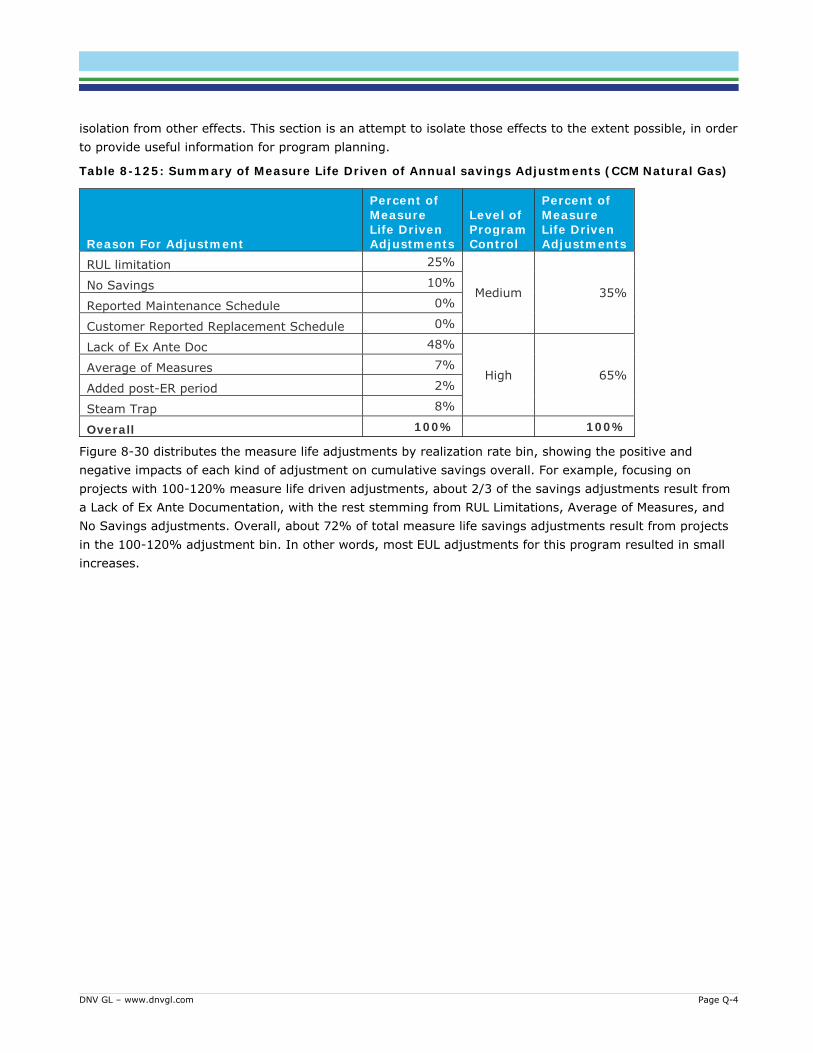
DNV GL – www.dnvgl.com Page Q-4
isolation from other effects. This section is an attempt to isolate those effects to the extent possible, in order to provide useful information for program planning.
Table 8-125: Summary of Measure Life Driven of Annual savings Adjustments (CCM Natural Gas)
Reason For Adjustment
Percent of Measure Life Driven Adjustments
Level of Program Control
Percent of Measure Life Driven Adjustments
RUL limitation 25%
Medium 35% No Savings 10%
Reported Maintenance Schedule 0%
Customer Reported Replacement Schedule 0%
Lack of Ex Ante Doc 48%
High 65% Average of Measures 7%
Added post-ER period 2%
Steam Trap 8%
Overall 100% 100%
Figure 8-30 distributes the measure life adjustments by realization rate bin, showing the positive and negative impacts of each kind of adjustment on cumulative savings overall. For example, focusing on projects with 100-120% measure life driven adjustments, about 2/3 of the savings adjustments result from a Lack of Ex Ante Documentation, with the rest stemming from RUL Limitations, Average of Measures, and No Savings adjustments. Overall, about 72% of total measure life savings adjustments result from projects in the 100-120% adjustment bin. In other words, most EUL adjustments for this program resulted in small increases.

DNV GL – www.dnvgl.com Page Q-5
Figure 8-30: EUL Adjustments by Magnitude of Adjustment (CCM Natural Gas)
Figure 8-31 shows the level of program control over the adjustments shown in Figure 8-30. For example, the program has a “High” level of control over most reasons which resulted in adjustments of 100-120%.

DNV GL – www.dnvgl.com Page Q-6
Figure 8-31: Program Control Over Measure Life Driven Savings Adjustments by Magnitude of Adjustment (CCM Natural Gas)
Union Commercial, Industrial and Multi-Family
Annual savings adjustments The total absolute value of the annual savings adjustments (engineering adjustment) for Union Custom Programs are 2,652,557 m3 of natural gas, or 3% of the total first year sample tracking savings of 85,649,059 m3. The engineering adjustment represents the differences in ex post and ex ante savings that are not a result of the influence correction. These changes are due to differences in calculation methods, EUL, calculation parameters, or other engineering-related adjustments.
Table 8-126 shows the percent of total annual savings adjustments associated with each Reason for Adjustment. The table also indicates the level of control that the program has over that discrepancy through improved calculations or improved documentation, as discussed in Table 8-122. For example, “Efficient Equipment Operating Conditions” represents 75% of first year discrepancies, and the program has a limited (“Low”) ability to prevent this kind of adjustment. The table shows that 90% of adjustments to Union’ Custom programs were issues that the program likely has a low ability to control.

DNV GL – www.dnvgl.com Page Q-7
Table 8-126: Summary of Annual savings Adjustments
Reason For Adjustment Percent of First Year Discrepancy
Level of Program Control
Percent of First Year Discrepancy
Measured Usage 0%
Low 90% Efficient Equipment Operating Conditions 75%
Operating Hours 15%
Change to Calculation Method 3% Medium 4%
Baseline 1%
Efficient Equipment Specifications 1% High 6%
Data Entry Error 4%
Overall 100% 100%
Figure 8-32 distributes the annual savings adjustments by realization rate bin, showing the positive and negative impacts of each adjustment on first year program savings. Overall, adjustments were mostly because of changes to Efficient Equipment Operating Conditions and Operating Hours.
Figure 8-32: Annual savings Adjustments by Magnitude of Adjustment (m3 Natural Gas)
Figure 8-33 shows the level of program control over the adjustments shown in Figure 8-32. Almost all first-year savings discrepancies were in categories that the program has a low degree of control over.

DNV GL – www.dnvgl.com Page Q-8
Figure 8-33: Program Control Over Annual savings Adjustments by Magnitude of Adjustment (m3
Natural Gas)
Measure life adjustments Total absolute value measure life driven cumulative savings adjustments for Union Custom Programs are 31,801,957 CCM of natural gas, or 2% of the total cumulative sample tracking savings of 1,277,857,163 CCM. These are cumulative lifetime savings41 and should not be compared to annual savings adjustments.
Table 8-127 shows the percent of total measure life-driven adjustments associated with each specific Reason for Adjustment. The table also indicates the level of control that the program has over that discrepancy through improved calculations or improved documentation, as discussed in Table 8-123. The table shows that 85% of EUL adjustments were due to categories that the program has a high degree of control over. However, this effect is likely overstated because weighting EUL adjustments by ex ante savings may overstate some changes. For example, many Union sites received significant EUL adjustments for early replacement projects that installed ISP technologies. Although the total EUL was greatly increased, the post-ER savings were zero. Using the ex post savings to weight those measures would likely result in a different distribution.
Note that measure life adjustments shown here are inexact. Because they result from changes to both RUL and EUL, there is no way to directly compare the impacts of measure life changes on savings in isolation
41 To provide comparable values, the cumulative savings adjustments are calculated as ex ante annual savings times ex post EUL minus ex ante
annual savings times ex ante EUL.

DNV GL – www.dnvgl.com Page Q-9
from other effects. This section is an attempt to isolate those effects to the extent possible, in order to provide useful information for program planning.
Table 8-127: Summary of Measure Life Driven of Annual savings Adjustments (CCM Natural Gas)
Reason For Adjustment
Percent of Measure Life Driven Adjustments
Level of Program Control
Percent of Measure Life Driven Adjustments
RUL limitation 15%
Medium 15% No Savings 0%
Reported Maintenance Schedule 0%
Customer Reported Replacement Schedule 0%
Lack of Ex Ante Doc 34%
High 85% Average of Measures 0%
Added post-ER period 49%
Steam Trap 1%
Overall 100% 100.0%
Figure 8-34 distributes the measure life adjustments by realization rate bin, showing the positive and negative impacts of each kind of adjustment on cumulative savings overall. The figure shows that most of the EUL adjustments were small and positive, while a few were strongly negative.
Figure 8-34: Measure Life Driven Savings Adjustments by Magnitude of Adjustment (CCM Natural Gas)

DNV GL – www.dnvgl.com Page Q-10
Figure 8-35 shows the level of program control over the adjustments shown in Figure 8-34. For example, the program has a “High” level of control over most reasons which resulted in adjustments of 100-120%.
Figure 8-35: Program Control Over Measure Life Driven Savings Adjustments by Magnitude of Adjustment (CCM Natural Gas)
Union Large Volume
Annual savings adjustments Total absolute value annual savings adjustments (engineering adjustment) for Union Large Volume are 54,809,839 m3 of natural gas, or 74% of the total first year sample tracking savings of 73,711,036 m3. The engineering adjustment represents the differences in ex post and ex ante savings that are not a result of the influence correction.
Table 8-128 shows the percent of total annual savings adjustments associated with each Reason for Adjustment. The table also indicates the level of control that the program has over that discrepancy through improved calculations or improved documentation, as discussed in Table 8-122. For example, “Efficient Equipment Operating Conditions” represents 57% of first year discrepancies, and the program has a limited (“Low”) ability to prevent this kind of adjustment. The table shows that discrepancies classified as data entry errors had a significant effect on adjustments. Seven sites had adjustments of this type, with three of them being caused by transfer of values from the project workbook to the tracking database. These are separate from the Influence Adjustments applied by Union to some projects, which are removed from ex ante savings and not considered here.

DNV GL – www.dnvgl.com Page Q-11
Table 8-128: Summary of Annual savings Adjustments
Reason For Adjustment Percent of First Year Discrepancy
Level of Program Control
Percent of First Year Discrepancy
Measured Usage 5%
Low 66% Efficient Equipment Operating Conditions 57%
Operating Hours 4%
Change to Calculation Method 0% Medium 1%
Baseline 1%
Efficient Equipment Specifications 0% High 33%
Data Entry Error 33%
Overall 100% 100%
Figure 8-36 distributes the annual savings adjustments by realization rate bin, showing the positive and negative impacts of each adjustment on first year program savings. The figure shows that most of the annual savings adjustments were large and positive.
Figure 8-36: Annual savings Adjustments by Magnitude of Adjustment (m3 Natural Gas)
Figure 8-37 shows the level of program control over the adjustments shown in Figure 8-36. As with previous programs, almost all annual savings discrepancies are in areas the program has low control over.

DNV GL – www.dnvgl.com Page Q-12
Figure 8-37: Program Control Over Annual savings Adjustments by Magnitude of Adjustment (m3
Natural Gas)
Measure life adjustments Total measure life driven cumulative savings adjustments for Union Large Volume are 384,999,510 CCM of natural gas, or 45% of the total first year sample tracking savings of 856,320,533 CCM. These are cumulative lifetime savings42 and should not be compared to annual savings adjustments.
Table 8-129 shows the percent of total measure life-driven adjustments associated with each specific Reason for Adjustment. The table also indicates the level of control that the program has over that discrepancy through improved calculations or improved documentation, as discussed in Table 8-123. The table shows that 65% of the adjustments made to measure life for the Large Volume program are in areas of high program control. However, this effect is likely overstated because weighting EUL adjustments by ex ante savings may overstate some changes. For example, many Union sites received significant EUL adjustments for early replacement projects that installed ISP technologies. Although the total EUL was greatly increased, the post-ER savings were zero. Using the ex post savings to weight those measures would likely result in a different distribution.
Note that measure life adjustments shown here are inexact. Because they result from changes to both RUL and EUL, there is no way to directly compare the impacts of measure life changes on savings in isolation
42 To provide comparable values, the cumulative savings adjustments are calculated as ex ante annual savings times ex post EUL minus ex ante
annual savings times ex ante EUL.

DNV GL – www.dnvgl.com Page Q-13
from other effects. This section is an attempt to isolate those effects to the extent possible, in order to provide useful information for program planning.
Table 8-129: Summary of measure-life-driven annual savings adjustments (CCM natural gas)
Reason for Adjustment
Percent of Measure
Life Driven Adjustments
Level of Program Control
Percent of Measure
Life Driven Adjustments
RUL limitation 10%
Medium 35% No Savings 9% Reported Maintenance Schedule <1% Customer Reported Replacement Schedule 16% Lack of Ex Ante Doc 10%
High 65% Average of Measures 0% Added post-ER period 54% Steam Trap <1% Overall 100% 100%
Figure 8-38 distributes the measure life adjustments by realization rate bin, showing the positive and negative impacts of each kind of adjustment on cumulative savings overall. The figure shows that most of the EUL adjustments were small and positive while a few were extremely positive or extremely negative.

DNV GL – www.dnvgl.com Page Q-14
Figure 8-38: Measure-life-driven savings adjustments by magnitude of adjustment (CCM natural gas)
Figure 8-39 shows the level of program control over the adjustments shown in Figure 8-38. For example, the program has a “High” level of control over most reasons which resulted in adjustments of 100-120%.

DNV GL – www.dnvgl.com Page Q-15
Figure 8-39: Program control over measure-life-driven savings adjustments by magnitude of adjustment (CCM Natural Gas)

About DNV GL Driven by our purpose of safeguarding life, property and the environment, DNV GL enables organizations to advance the safety and sustainability of their business. We provide classification and technical assurance along with software and independent expert advisory services to the maritime, oil and gas, and energy industries. We also provide certification services to customers across a wide range of industries. Operating in more than 100 countries, our 16,000 professionals are dedicated to helping our customers make the world safer, smarter and greener.

About DNV GL Driven by our purpose of safeguarding life, property and the environment, DNV GL enables organizations to advance the safety and sustainability of their business. We provide classification and technical assurance along with software and independent expert advisory services to the maritime, oil and gas, and energy industries. We also provide certification services to customers across a wide range of industries. Operating in more than 100 countries, our 16,000 professionals are dedicated to helping our customers make the world safer, smarter and greener.