2016 annual technology baseline (atb), nrel (national
TRANSCRIPT

Notes pages provide additional detail and are essential for interpreting information on slides.Excel spreadsheet accompanies this documentation and contains all input data and calculations illustrated on subsequent pages.
All monetary values presented in 2014 U.S. dollars. Inflation rates for converting between dollar years were determined using the consumer price index as published by the U.S. Bureau of Labor and Statistics.
Recommended citation:NREL (National Renewable Energy Laboratory). 2016. 2016 Annual Technology Baseline. Golden, CO: National Renewable Energy Laboratory. http://www.nrel.gov/analysis/data_tech_baseline.html.
1
2

3

4

PrefaceThis presentation is one of several products resulting from an effort to provide a consistent set of technology cost and performance data and to define a conceptual and consistent scenario framework that can be used in NREL’s future analyses. The long‐term objective of this effort is to identify a range of possible futures of the U.S. electricity sector in which to consider specific energy system issues through (1) defining a set of prospective scenarios that bound ranges of key technology, market, and policy assumptions; and (2) assessing these scenarios in NREL’s market models to understand the range of resulting outcomes, including energy technology deployment and production, energy prices, and CO2 emissions.
The effort, supported by the U.S. Department of Energy’s (DOE) Office of Energy Efficiency and Renewable Energy (EERE), has focused on the electric sector by creating a technology cost and performance database, defining scenarios, documenting associated assumptions, and generating modeled results using NREL’s Regional Energy Deployment Systems Model (ReEDS). This work leverages and continues significant activity already being funded by EERE for individual technologies and market segments. The specific products includes the following:
• An Annual Technology Baseline (ATB) workbook documenting detailed cost and performance data (both current and projected) for both renewable and conventional technologies.
• This ATB summary presentation describing each of the technologies and providing additional context for their treatment in the workbook.
• A 2016 Standard Scenarios Annual Report describing the identified scenarios, associated assumptions (including technology cost and performance assumptions from the ATB), modeled results, and the base structure of the specific version of the ReEDS model (v2016.1) (annual “release”) used to generate the results.
These products can be accessed at http://www.nrel.gov/analysis/data_tech_baseline.html.
NREL intends to consistently apply these products in its ongoing electric sector scenarios analyses to ensure that the analyses incorporate a transparent, realistic, and timely set of input assumptions and consider a diverse set of potential futures. The application of standard scenarios, clear documentation of underlying assumptions, and model versioning is expected to result in
• improved transparency of critical input assumptions and modeling methodologies;• improved comparability of results across studies;• improved consideration of the potential economic and environmental impacts of generation technology
improvement, changes in market conditions, and changes to policies and regulations; and • an enhanced framework for formulating and addressing new analysis questions.
NREL plans to update the scenario framework and technology baseline annually and extend it to other technologies, models, and sectors, including transportation and the built environment.
5

These examples of recent NREL scenario analyses all required technology cost and performance assumptions, and motivated the creation of the ATB in order to improve the consistency across the analyses.
6

With the increased reliance on NREL's data and modeling tools for studies for EERE and other stakeholders, we collectively recognized the need and opportunity to establish a process to develop and communicate the underlying data and assumptions on which they are based.
Scenario analyses have become an integral component of the technology analysis portfolio conducted at the DOE and NREL, and are used to inform long‐term R&D strategies. The cost and performance of technologies today and into the future are critical drivers of the evolution of the power system. Transparent, harmonized assumptions are crucial for conducting robust scenario analysis to inform R&D strategies.
7
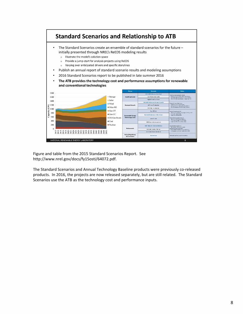
Figure and table from the 2015 Standard Scenarios Report. See http://www.nrel.gov/docs/fy15osti/64072.pdf.
The Standard Scenarios and Annual Technology Baseline products were previously co‐released products. In 2016, the projects are now released separately, but are still related. The Standard Scenarios use the ATB as the technology cost and performance inputs.
8

LCOE is used throughout this deck as a summary metric for the various cost and performance inputs of each technology. More information on the LCOE can be found in the “Summary of Technologies” section.
9

• ATB Methodology for Fossil and Nuclear Generation Plants• Rely on EIA representation of current year plant cost estimates, and for plant cost
projections through 2040 (AEO 2016)• Rely on EIA scenarios for fuel price projections through 2040 (AEO 2016)• Linearly extrapolate the EIA plant cost estimates from 2040 through 2050 • Hold the EIA fuel price projections at 2040 levels through 2050
• ATB Methodology for Biopower Plants• Rely on EIA representation of current year plant cost estimates• Rely on EIA representation of future plant cost estimates through 2040 (AEO 2016)• Linearly extrapolate the EIA plant cost estimates from 2040 through 2050 • Represent average biopower feedstock price based on “Billion Ton Study” through 2030• Hold the biopower feedstock price at 2030 levels through 2050
ReferencesU.S. Energy Information Administration. (2016). Annual Energy Outlook 2016 Early Release. May 2016.
DOE. (2011). US Billion‐Ton Update: Biomass Supply for a Bioenergy and BioproductsIndustry. ORNL/TM‐2011/224.
10

References:DOE Wind Vision 2015: Wind Cost Appendix H: Table H‐4.Feldman et al (2015) Photovoltaic System Pricing Trends: 2015 Edition. NREL/PR‐6A20‐64898.Kurup, P and Turchi, C. (2015), Parabolic Trough Collector Cost Update for the System Advisor Model (SAM). NREL Report No. TP‐6A20‐65228.US DOE Geothermal Energy Technology Evaluation Model (GETEM). http://www4.eere.energy.gov/geothermal/projects/1096 and http://www4.eere.energy.gov/geothermal/sites/default/files/documents/mines_getem_peer2013.pdf.O’Connor, P.W., S.T. DeNeale, D.R. Chalise, A. Maloof (2015). Hydropower Baseline Cost Modeling, Version 2. ORNL/TM‐2015/471. Oak Ridge, TN: Oak Ridge National Laboratory. Electricity Market Module in Assumptions to AEO 2015: Table 8.2.U.S. Energy Information Administration. (2016). Annual Energy Outlook 2016 Early Release. May 2016.
11
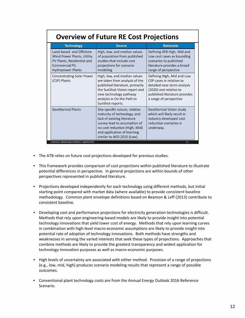
• The ATB relies on future cost projections developed for previous studies.
• This framework provides comparison of cost projections within published literature to illustrate potential differences in perspective. In general projections are within bounds of other perspectives represented in published literature.
• Projections developed independently for each technology using different methods, but initial starting point compared with market data (where available) to provide consistent baselinemethodology. Common plant envelope definitions based on Beamon & Leff (2013) contribute to consistent baseline.
• Developing cost and performance projections for electricity generation technologies is difficult. Methods that rely upon engineering‐based models are likely to provide insight into potential technology innovations that yield lower cost of energy. Methods that rely upon learning curves in combination with high‐level macro‐economic assumptions are likely to provide insight into potential rate of adoption of technology innovations. Both methods have strengths and weaknesses in serving the varied interests that seek these types of projections. Approaches that combine methods are likely to provide the greatest transparency and widest application for technology innovation purposes as well as macro‐economic purposes.
• High levels of uncertainty are associated with either method. Provision of a range of projections (e.g., low, mid, high) produces scenario modeling results that represent a range of possible outcomes.
• Conventional plant technology costs are from the Annual Energy Outlook 2016 Reference Scenario.
12

13

14

15

• Total land‐based wind potential exceeds 10,000 GW corresponding to over 3.5M square kilometers of potential land area after accounting for standard exclusions such as federally protected areas, urban areas, water, and others. Resource potential has been expanded from approximately 6,000 GW (DOE 2015) by including locations with lower wind speeds to provide more comprehensive coverage of US land areas where future technology may improve economic potential.
• Resource potential represented by over 130,000 distinct “areas” for wind plant deployment covering over 3.5M square kilometers; potential capacity estimated assuming 3 MW/km2 to total over 10,000 GW
• CAPEX based on one of three turbine models associated with the annual average wind speed for each “area”.
• CF determined using three normalized wind turbine power curves and hourly wind profile for each “area”• The majority of land‐based wind plants installed in the U.S. range from 50 MW to 100 MW (Wiser and
Bolinger, 2014).
References• DOE (2015). Wind Vision: A New Era for Wind Power in the United States. 288 pp.; Department of Energy
Report No. DOE/GO‐102015‐4557. http://energy.gov/sites/prod/files/2015/03/f20/wv_full_report.pdf
• Volume 2: Renewable Electricity Generation and Storage Technologies• Augustine, C.; Bain, R.; Chapman, J.; Denholm, P.; Drury, E.; Hall, D.G.; Lantz, E.; Margolis, R.; Thresher, R.;
Sandor, D.; Bishop, N.A.; Brown, S.R.; Cada, G.F.; Felker, F.; Fernandez, S.J.; Goodrich, A.C.; Hagerman, G.; Heath, G.; O’Neil, S.; Paquette, J.; Tegen, S.; Young, K. (2012). Renewable Electricity Generation and Storage Technologies. Vol 2. of Renewable Electricity Futures Study. NREL/TP‐6A20‐52409‐2. Golden, CO: National Renewable Energy Laboratory.
• AWS Truepower. Wind Resource Map. https://www.awstruepower.com/assets/Wind‐Resource‐Map‐UNITED‐STATES‐11x171.pdf
• Wiser, R.; Bolinger, M.; Barbose, G.; Darghouth, N.; Hoen, B.; Mills, A.; Weaver, S.; Porter, K.; Buckley, M.; Oteri, F.; Tegen, S. (2014). 2013 Wind Technologies Market Report. 96 pp.; NREL Report No. TP‐5000‐62345; DOE/GO‐102014‐4459.
16

• CAPEX in ATB represents wind plant cost in location with no significant logistical challenges or unusual siting conditions similar to the Interior region of the U.S. Regional variants associated with labor rates, material costs, etc. (CapRegMult) are not included.
• CAPEX represents total expenditure required to achieve commercial operation in a given year. Plant envelope defined to include the following (Beamon and Leff, 2013; Moné et al., 2015):
• Wind turbine supply • Balance of System including
• turbine installation, substructure supply and installation• site preparation, installation of underground utilities, access roads, buildings for operations and maintenance• electrical infrastructure such as transformers, switchgear and electrical system connecting turbines to each
other and to control center• project indirect costs including engineering, distributable labor and materials, construction management
start up and commissioning, and contractor overhead costs, fees and profit.• Financial Costs
• owner’s costs such as development costs, preliminary feasibility and engineering studies, environmental studies and permitting, legal fees, insurance costs, property taxes during construction
• onsite electrical equipment (e.g., switchyard), a nominal‐distance spur line (<1 mi), and necessary upgrades at a transmission substation; distance‐based spur line cost (GCC) not included in ATB.
• interest during construction estimated based on 3‐year duration accumulated 10%/10%/80% at half‐year intervals and 8% interest rate
• ATB spreadsheet input is Overnight Capital Cost (OCC) and details to calculate interest during construction (ConFinFactor).
Standard Scenarios Model Results• CAPEX in ATB does not represent regional variants (CapRegMult) associated with labor rates, material costs, etc., but ReEDS does
include 134 regional multipliers (Beamon and Leff, 2013)• ReEDS determines land‐based spur line (GCC) uniquely for each of the 130,000 “areas” based on distance and transmission line
cost.
References• Beamon, A.; Leff. M. (2013). EOP III Task 1606, Subtask 3 – Review of Power Plant Cost and Performance Assumptions for NEMS.
Prepared by SAIC Energy, Environment & Infrastructure, LLC for the Energy Information Administration, Office of Energy Analysis.http://www.eia.gov/forecasts/capitalcost/pdf/updated_capcost.pdf
• Moné, C.; Smith, A., Hand, M., Maples, B. (2015). 2013 Cost of Wind Energy Review. http://www.nrel.gov/docs/fy15osti/63267.pdf
17

• For illustration in ATB, all potential land‐based wind plant “areas” were represented in ten techno‐resource groups (TRG). Ten TRG’s were defined by resource potential (GW) and with higher resolution on the highest quality TRGs as these are the most likely sites to be deployed, based on their economics.
• TRG 1 represents the best 100 GW of wind, as determined by LCOE, TRG 2 represents the next best 200 GW, TRG 3 represents the next best 400 GW and TRG 4 represents the next best 800 GW. TRGs 5‐9 all represent 1600 GW of resource potential. TRG 10 represents the remaining 1140 GW of available potential. LCOEs associated with this range of resource potential varies from about $47/MWh to $228/MWh in 2014. This representation is based on the approach described in (DOE 2015), but defines the resource in terms of 10 TRGs rather than 5 to improve resolution and accommodate the increased resource potential at lower wind speeds.
• The table below summarizes the annual average wind speed range for each TRG, capacity weighted average wind speed, cost and performance parameters for each TRG, and resource potential in terms of capacity and energy for each TRG
• Actual land‐based wind plant CAPEX (Wiser and Bolinger, 2014) is shown in box and whiskers format (bar represents median, box represents 25th and 75th percentile, whiskers represent minimum and maximum; diamond represents capacity weighted average) for comparison to ATB current CAPEX estimates and future projections. Wiser & Bolinger (2014) provides statistical representation of CAPEX for about 65% of wind plants installed in the U.S. since 2007
• CAPEX estimates for 2014 correspond well with market data for plants installed in 2014. Projections reflect continuation of downward trend observed in recent past and anticipated to continue based on preliminary data for 2015 projects.
• CAPEX estimates should tend toward the low end of observed cost because no regional impacts or spur line costs are included. These effects are represented in the market data.
• Projections of future wind plant CAPEX were determined based on adjustments to CAPEX, FOM and CF in each year to result in a pre‐determined LCOE value. In the lower wind resource areas represented by TRGs 6‐10 CAPEX is likely to grow as future wind turbine technology transitions to new platforms including taller towers, larger rotors and higher machine ratings. In the higher wind resource areas represented by TRGs 1‐5 optimization of current wind turbine platforms will lead to lower CAPEX.
References• Wiser, R.; Bolinger, M.; Barbose, G.; Darghouth, N.; Hoen, B.; Mills, A.; Weaver, S.; Porter, K.; Buckley, M.; Oteri, F.; Tegen, S. (2014). 2013 Wind
Technologies Market Report. 96 pp.; NREL Report No. TP‐5000‐62345; DOE/GO‐102014‐4459.• Lantz, E.; Wiser, R.; Hand, M. (2012). IEA Wind Task 26: The Past and Future Cost of Wind Energy, Work Package 2. 137 pp.; NREL Report No. TP‐6A20‐
53510.• Wiser, R.; Lantz, E.; Bolinger, M.; Hand, M. (2012). Recent Developments in the Levelized Cost of Energy From U.S. Wind Power Projects. Presentation
submitted to IEA Task 26. • DOE (2015). Wind Vision: A New Era for Wind Power in the United States. 288 pp.; Department of Energy Report No. DOE/GO‐102015‐4557.
http://energy.gov/sites/prod/files/2015/03/f20/wv_full_report.pdf
18
Wind Speed Range (m/s)
Weighted Average Wind Speed (m/s)
Weighted Average CAPEX
($/kW)
Weighted Average OPEX
($/kW/yr)
Weighted Average Net CF
(%)
Potential Wind Plant Capacity
(GW)
Potential Wind Plant Energy
(TWh)
7.7 - 13.5 8.8 1737 51 51% 100 4117.5 - 10.4 8.3 1775 51 49% 200 8097.3 - 10.5 8.1 1778 51 48% 400 16107.1 - 10.1 7.9 1783 51 47% 800 31996.8 - 9.5 7.5 1833 51 45% 1600 623861. - 9.4 6.9 1867 51 40% 1600 55675.3 - 8.3 6.2 1895 51 33% 1600 45614.7 - 6.6 5.5 1930 51 26% 1600 35134.1 - 5.7 4.8 1999 51 20% 1600 25971.6 - 5.1 4.0 2109 51 12% 1140 1099
10,640 29606
Techno-Resource Group (TRG)
Total
TRG1TRG2TRG3TRG4TRG5TRG6TRG7TRG8TRG9
TRG10

• Represent annual fixed expenditures (depend on capacity) required to operate and maintain a wind plant over its technical lifetime of 25 years including
• Insurance, taxes, land lease payments, and other fixed costs• Present value, annualized large component replacement costs over technical life (e.g.
blades, gearboxes, generators)• Scheduled and unscheduled maintenance of wind plant components including turbines,
transformers, etc. over technical lifetime• Due to lack of robust market data, assumption of $51/kW/yr determined to be representative of
range of available data; no variation with TRG (or wind speed). • Projections of future wind plant FOM were determined based on adjustments to CAPEX, FOM
and CF in each year to result in a pre‐determined LCOE value.
References• Lantz, E. (2013). Operations Expenditures: Historical Trends and Continuing Challenges
(Presentation). NREL (National Renewable Energy Laboratory). 20 pp.; NREL Report No. PR‐6A20‐58606.
• Wiser, R.; Bolinger, M.; Barbose, G.; Darghouth, N.; Hoen, B.; Mills, A.; Weaver, S.; Porter, K.; Buckley, M.; Oteri, F.; Tegen, S. (2014). 2013 Wind Technologies Market Report. 96 pp.; NREL Report No. TP‐5000‐62345; DOE/GO‐102014‐4459.
• DOE (2015). Wind Vision: A New Era for Wind Power in the United States. 288 pp.; Department of Energy Report No. DOE/GO‐102015‐4557. http://energy.gov/sites/prod/files/2015/03/f20/wv_full_report.pdf
19

• Capacity factor represents expected annual average energy production divided by annual energy production assuming the plant operates at rated capacity for every hour of the year. Intended to represent long‐term average over technical lifetime of plant and does not represent inter‐annual variation in energy production.
• CF influenced by rotor swept area / generator capacity, hub height, hourly wind profile, expected downtime, energy losses within wind plant
• CF referenced to 80 m above ground level long‐term average hourly wind resource data from AWS Truepower• For illustration in ATB, all potential land‐based wind plant “areas” were represented in ten TRGs. Capacity weighted
average CAPEX, CF, and resource potential are shown in earlier slide. (DOE 2015).• Actual energy production from about 90% of wind plants operating in the U.S. since 2007 (Wiser and Bolinger, 2014)
is shown in box and whiskers format for comparison with ATB current estimates and future projections. The historic data illustrates capacity factor for projects operating in 2014 shown by year of commercial online date. A wind index developed by NextEra is used to normalize wind energy production in 2014 relative to historic average wind energy production.
• Majority of installed U.S. wind plants generally aligned with ATB estimates for performance in TRGs 5‐7. High wind resource sites associated with TRGs 1‐4 as well as very low wind resource sites associated with TRGs 8‐10 are not as common in historic data, but the range of observed data encompasses ATB estimates. Projections of capacity factor for plants installed in future years were determined based on adjustments to CAPEX, FOM and CF in each year to result in a pre‐determined LCOE value (see next slide for description of methodology).
• Projections for capacity factors implicitly reflect technology innovations such as larger rotors and taller towers that will increase energy capture at the same geographic location without specifying precise tower height and rotor diameter changes.
Standard Scenarios Model Results• ReEDS output capacity factors for wind and solar‐PV can be lower than input capacity factors due to endogenously
estimated curtailments determined by scenario constraints.
References• Wiser, R.; Bolinger, M.; Barbose, G.; Darghouth, N.; Hoen, B.; Mills, A.; Weaver, S.; Porter, K.; Buckley, M.; Oteri, F.;
Tegen, S. (2014). 2013 Wind Technologies Market Report. 96 pp.; NREL Report No. TP‐5000‐62345; DOE/GO‐102014‐4459.
• Lantz, E.; Wiser, R.; Hand, M. (2012). IEA Wind Task 26: The Past and Future Cost of Wind Energy, Work Package 2. 137 pp.; NREL Report No. TP‐6A20‐53510.
• Wiser, R.; Lantz, E.; Bolinger, M.; Hand, M. (2012). Recent Developments in the Levelized Cost of Energy From U.S. Wind Power Projects. Presentation submitted to IEA Task 26.
• DOE (2015). Wind Vision: A New Era for Wind Power in the United States. 288 pp.; Department of Energy Report No. DOE/GO‐102015‐4557. http://energy.gov/sites/prod/files/2015/03/f20/wv_full_report.pdf
20

• Projections derived from broad‐based literature review (DOE 2015) and vetted with a consortium of National Laboratory, DOE and wind industry experts.
• Projections derived from analysis of more than 20 different projection scenarios from more than 15 independent published studies.
• Literature estimates normalized to a common 2014 starting point in order to focus on projected cost reduction instead of absolute reported costs; range of cost reduction 0% ‐ 40% through 2050.
• Three different projections developed for scenario modeling as bounding levels• Low Wind Cost: Maximum annual cost reduction based on literature• Mid Cost: Median annual cost reduction identified in the literature• High Wind Cost: No change in LCOE from 2014 ‐ 2050
• Cost of energy reductions were implemented as changes to CAPEX, CF, and FOM as illustrated on previous slides.
References• Lantz, E.; Wiser, R.; Hand, M. (2012). IEA Wind Task 26: The Past and Future Cost of Wind
Energy, Work Package 2. 137 pp.; NREL Report No. TP‐6A20‐53510.• DOE (2015). Wind Vision: A New Era for Wind Power in the United States. 288 pp.; Department
of Energy Report No. DOE/GO‐102015‐4557. http://energy.gov/sites/prod/files/2015/03/f20/wv_full_report.pdf
21

In general, projections represent the following trends, and the degree of adoption distinguishes between Low and Mid Wind Cost scenarios.
• Continued turbine scaling to larger MW turbines with larger rotors such that swept area / MW capacity decreases resulting in high capacity factors for a given location
• Continued diversity of turbine technology where largest rotor diameter turbines tend to be located in lower wind speed sites, but number of turbine options for higher wind speed sites increases.
• Taller towers that result in higher capacity factors for a given site due to wind speed increase with elevation above ground level.
• Improved plant siting and operation to reduce plant level energy losses increasing capacity factor.
• More efficient operation and maintenance procedures combined with more reliable components to reduce annual average FOM costs.
• Continued manufacturing and design efficiencies such that capital cost / kW decreases with larger turbine components.
• Adoption of a wide range of innovative control, design, and material concepts that facilitate the high level trends described above.
22

23

• Wind resource prevalent along U.S. coastal areas including the Great Lakes . Resource potential exceeds 1500 GW (Hand et al., forthcoming) after accounting for exclusions such as marine protected areas, shipping lanes, pipelines, and others.
• Resource potential represented by over 30,000 “areas” for wind plant deployment; potential capacity estimated assuming 3 MW/km2 to total over 15 00 GW.
• CAPEX estimates for each “area” based on one turbine model with three sub‐structure concepts associated with three ranges of water depth
• Substructure type reflects water depth• Monopile – shallow water from 0‐30 m• Jacket – mid‐depth from 31‐60 m• Floating – deep water from 61‐700 m
• CF estimates determined based on one normalized wind turbine power curve and hourly wind profile for each “area”
• Representative offshore wind plant size is assumed to be about 500 MW (Tegen et al., 2012)
References• DOE (2015). Wind Vision: A New Era for Wind Power in the United States. 288 pp.; Department
of Energy Report No. DOE/GO‐102015‐4557. http://energy.gov/sites/prod/files/2015/03/f20/wv_full_report.pdf
• Moné, C.; Stehly, T., Maples, B., Settle, E. (2015). 2014 Cost of Wind Energy Review. http://www.nrel.gov/docs/fy16osti/64281.pdf
24

• CAPEX in ATB represents typical offshore wind plant sited 30 km from shore which is representative of currently installed European offshore wind plants. CAPEX in ATB does not explicitly represent regional variants associated with labor rates, material costs, etc. or geographically determined spur line costs.
• CAPEX for offshore wind plants in ATB include export cable costs and construction‐period transit costs associated with a representative distance of 30 km from shore (GCC based on 30 km distance).
• CAPEX represents total expenditure required to achieve commercial operation in a given year. Plant envelope defined to include the following (Beamon and Leff, 2013; Moné et al., 2015):
Wind turbine supply Balance of System including
turbine installation, substructure supply and installationsite preparation, port and staging area support for delivery, storage, handling, installation of underground utilitieselectrical infrastructure such as transformers, switchgear and electrical system connecting turbines to each other and to control centerproject indirect costs including engineering, distributable labor and materials, construction management start up and commissioning, and contractor overhead costs, fees and profit.
Financial Costsowner’s costs such as development costs, preliminary feasibility and engineering studies, environmental studies and permitting, legal fees, insurance costs, property taxes during constructiononsite electrical equipment (e.g., switchyard), a nominal‐distance spur line (<1 mi), and necessary upgrades at a transmission substationinterest during construction estimated based on 3‐year duration accumulated 10%/10%/80% at half‐year intervals and 8% interest rate
ATB spreadsheet input is Overnight Capital Cost (OCC) and details to calculate interest during construction (ConFinFactor).
Standard Scenarios Model Results• CAPEX in ATB does not represent regional variants (CapRegMult) associated with labor rates, material costs, etc.,
but ReEDS does include 134 regional multipliers (cite SAIC paper).• ReEDS determines offshore spur line and land‐based spur line (GCC) uniquely for each of the 30,000 “areas” based
on distance and transmission line cost. ReEDS includes estimates of associated incremental transportation costs during construction with the offshore spur line estimate.
ReferencesBeamon, A.; Leff. M. (2013). EOP III Task 1606, Subtask 3 – Review of Power Plant Cost and Performance Assumptions for NEMS. Prepared by SAIC Energy, Environment & Infrastructure, LLC for the Energy Information Administration, Office of Energy Analysis. http://www.eia.gov/forecasts/capitalcost/pdf/updated_capcost.pdf
Moné, C.; Smith, A., Hand, M., Maples, B. (2015). 2013 Cost of Wind Energy Review. http://www.nrel.gov/docs/fy15osti/63267.pdf
25

• For illustration in ATB, all potential offshore wind plant “areas” were represented in ten bins. The bins were defined based on water depth and LCOE range. Capacity weighted average wind speed and resource potential are shown below (DOE 2015).
• CAPEX in ATB represents offshore cable cost based on 30 km distance to land. • Actual and proposed offshore wind plant CAPEX (Smith et al., 2015) are shown in box and whiskers
format (bar represents median, box represents 25th and 75th percentile, whiskers represent minimum and maximum for comparison to ATB current CAPEX estimates and future projections.
• Historical CAPEX data represents European projects > 100 MW installed from 2001 to 2014. • CAPEX estimates for shallow and mid‐depth “areas” are comparable to market data; floating technology is
not yet commercial and no market comparison data exists.• Projections of future wind plant CAPEX were determined based on adjustments to CAPEX, FOM and CF in
each year to result in a pre‐determined LCOE value.
Reference• DOE (2015). Wind Vision: A New Era for Wind Power in the United States. 288 pp.; Department of Energy
Report No. DOE/GO‐102015‐4557. http://energy.gov/sites/prod/files/2015/03/f20/wv_full_report.pdf• Smith, A., Stehly, T., Musial, W. (2015). 2014‐2015 Offshore Wind Technologies Market Report. National
Renewable Energy Laboratory Report No. NREL/TP‐5000‐64283. Available at: http://www.nrel.gov/docs/fy15osti/64283.pdf
26
LCOE Range ($/MWh)Weighted
Average Wind Speed (m/s)
Potential Wind Plant Capacity
(GW)
Potential Wind Plant Energy
(TWh) OSW 1 LCOE <= 172 9.1 11 46OSW 2 172< LCOE <= 193 8.5 61 231OSW 3 193< LCOE <= 218 8 191 674OSW 4 218< LCOE 7.3 165 500OSW 5 LCOE <= 193 9.1 48 197OSW 6 193< LCOE <= 213 8.6 87 338OSW 7 213< LCOE 8.4 181 661OSW 8 LCOE <= 218 9.5 82 355OSW 9 218< LCOE <= 238 9 184 756
OSW 10 238< LCOE 8.6 549 20781,559 5835
TRG
Shallow (<= 30 m)
Mid-Depth (31-60 m)
Deep (61-700 m)
Total

• Represent annual fixed expenditures (depend on capacity) required to operate and maintain a wind plant over its technical lifetime of 25 years including
• Insurance, taxes, land lease payments, and other fixed costs• Present value, annualized large component replacement costs over technical life (e.g.
blades, gearboxes, generators)• Scheduled and unscheduled maintenance of wind plant components including turbines,
transformers, etc. over technical lifetime• Due to lack of robust market data, assumption of $134/kW/yr determined to be representative
of range of available data for fixed‐bottom offshore technologies (TRG 1‐7) and $165/kW/yr established to provide incremental cost for floating technologies (TRG 8‐10); no variation with wind speed.
• Projections of future wind plant FOM were determined based on adjustments to CAPEX, FOM and CF in each year to result in a pre‐determined LCOE value.
Reference• Tegen et al. 2012. Cost of Wind Energy Review.• DOE (2015). Wind Vision: A New Era for Wind Power in the United States. 288 pp.; Department
of Energy Report No. DOE/GO‐102015‐4557. http://energy.gov/sites/prod/files/2015/03/f20/wv_full_report.pdf
27

• Capacity factor represents expected annual average energy production divided by annual energy production assuming the plant operates at rated capacity for every hour of the year. Intended to represent long‐term average over technical lifetime of plant and does not represent inter‐annual variation in energy production.
• CF influenced by rotor swept area / generator capacity, hub height, hourly wind profile, expected downtime, energy losses within wind plant
• CF referenced to 80 m above water surface long‐term average hourly wind resource data from AWS Truepower
• For illustration in ATB, all potential offshore wind plant “areas” were represented in ten bins. The bins were defined based on water depth and LCOE ranges. Capacity weighted average CAPEX, CF, and resource potential are shown in earlier slide (DOE 2015).
• Actual energy production from wind plants operating in Europe (Smith et al., 2015) is shown in box and whiskers format for comparison with ATB current estimates and future projections. The historic data illustrates capacity factor for projects operating in 2014 shown by year of commercial online date.
• A majority of shallow to mid‐depth offshore wind plants with low to mid wind speeds in Europe are generally aligned with ATB estimates for performance (TRGs 2‐4, 6‐7, and 10). High wind resource sites ranging from shallow to deep water (TRGs 1, 5, and 8‐9) are not as common in historic data.
• Projections of capacity factor for plants installed in future years were determined based on adjustments to CAPEX, FOM and CF in each year to result in a pre‐determined LCOE value.
Standard Scenarios Model Results• ReEDS output capacity factors for wind and solar –PV can be lower than input capacity factors due to
endogenously estimated curtailments determined by scenario constraints.
References• DOE (2015). Wind Vision: A New Era for Wind Power in the United States. 288 pp.; Department of Energy
Report No. DOE/GO‐102015‐4557. http://energy.gov/sites/prod/files/2015/03/f20/wv_full_report.pdf• Smith, A., Stehly, T., Musial, W. (2015). 2014‐2015 Offshore Wind Technologies Market Report. National
Renewable Energy Laboratory Report No. NREL/TP‐5000‐64283. Available at: http://www.nrel.gov/docs/fy15osti/64283.pdf
28

• Projections derived from literature review (DOE 2015); data have been vetted broadly with wind industry participants.
• Projections derived from analysis of more than 10 different projection scenarios from 6 independent published studies.
• Fewer published offshore wind cost and performance projections exist, and most do not extend through 2050.
• Several pathways for cost reduction tied to specific technical advancements identified by BVG Associates for UK Crown Estate (BVG Associates 2012).
• Literature estimates normalized to a common starting point in order to focus on projected cost reduction; range of cost reduction 20‐50% through 2050. Due to lack of study projections extending beyond 2030, LCOE reductions post 2030 are loosely based on progress rates of 0% for High Cost and 5% for Mid and Low Cost.
• Relative cost of mid‐depth water plants and deep water, or floating, offshore wind plants maintained constant throughout scenario for simplicity; some hypothesize that unique aspects of floating technologies, such as ability to assemble and commission turbines at the port, could reduce cost relative to fixed‐bottom technologies.
• Three different projections developed for scenario modeling as bounding levels• Low Wind Cost: Maximum annual cost reduction based on literature, 51% by 2050• Mid Cost: Median annual cost reduction identified in the literature, 37% by 2050• High Wind Cost: Minimum annual cost reduction based on literature, 18% by 2050
• Cost of energy reductions were implemented as changes to CAPEX, CF, and FOM as illustrated on previous slides.
References
• DOE (2015). Wind Vision: A New Era for Wind Power in the United States. 288 pp.; Department of Energy Report No. DOE/GO‐102015‐4557. http://energy.gov/sites/prod/files/2015/03/f20/wv_full_report.pdf
• BVG Associates. (2012). Offshore Wind Cost Reduction Pathways: Technology Work Stream. The Crown Estate. London. Available at: http://www.thecrownestate.co.uk/media/305086/BVG%20OWCRP%20technology%20work%20stream.pdf
29
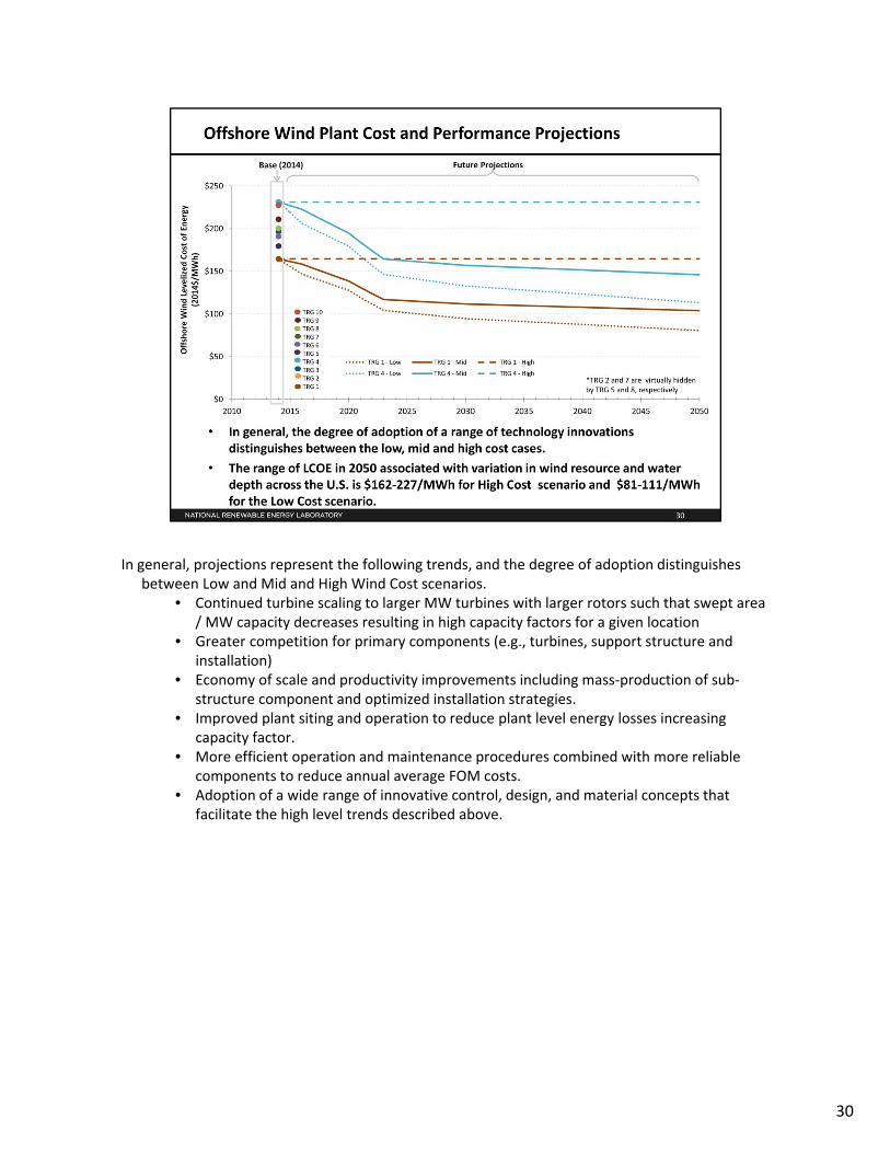
In general, projections represent the following trends, and the degree of adoption distinguishes between Low and Mid and High Wind Cost scenarios.
• Continued turbine scaling to larger MW turbines with larger rotors such that swept area / MW capacity decreases resulting in high capacity factors for a given location
• Greater competition for primary components (e.g., turbines, support structure and installation)
• Economy of scale and productivity improvements including mass‐production of sub‐structure component and optimized installation strategies.
• Improved plant siting and operation to reduce plant level energy losses increasing capacity factor.
• More efficient operation and maintenance procedures combined with more reliable components to reduce annual average FOM costs.
• Adoption of a wide range of innovative control, design, and material concepts that facilitate the high level trends described above.
30
31

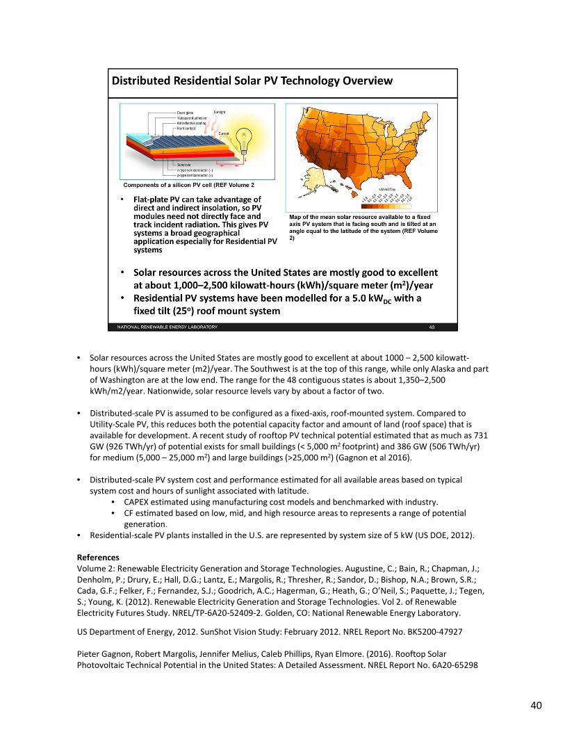
• Solar resources across the United States are mostly good to excellent at about 1,000–2,500 kilowatt‐hours (kWh)/square meter (m2)/year. The Southwest is at the top of this range, while only Alaska and part of Washington are at the low end. The range for the 48 contiguous states is about 1,350–2,500 kWh/m2/year. Nationwide, solar resource levels vary by about a factor of two.
• The total U.S. land area suitable for PV is significant and will not limit PV deployment. For example, one estimate suggested that the land area required to supply all end‐use electricity in the United States using PV is about 5,500,000 hectares (ha) (13,600,000 acres), which is equivalent to 0.6% of the country’s land area or about 22% of the “urban area” footprint (this calculation is based on deployment/land in all 50 states).
• Utility‐scale PV plant cost and performance estimated for all available areas based on typical plant cost and hours of sunlight associated with latitude.
• CAPEX estimated using manufacturing cost models and benchmarked with industry.• CF estimated based on hours of sunlight at latitude.
ReferencesVolume 2: Renewable Electricity Generation and Storage Technologies. Augustine, C.; Bain, R.; Chapman, J.; Denholm, P.; Drury, E.; Hall, D.G.; Lantz, E.; Margolis, R.; Thresher, R.; Sandor, D.; Bishop, N.A.; Brown, S.R.; Cada, G.F.; Felker, F.; Fernandez, S.J.; Goodrich, A.C.; Hagerman, G.; Heath, G.; O’Neil, S.; Paquette, J.; Tegen, S.; Young, K. (2012). Renewable Electricity Generation and Storage Technologies. Vol 2. of Renewable Electricity Futures Study. NREL/TP‐6A20‐52409‐2. Golden, CO: National Renewable Energy Laboratory.
32

• CAPEX in ATB represents solar PV plant cost based on modeled system prices representative of bids issued in the fourth quarter of the previous year.• CAPEX in ATB does not explicitly represent regional variants associated with labor rates, material costs, etc. or geographically determined spur lines costs.• CAPEX represents total expenditure required to achieve commercial operation in a given year. Plant envelope defined to include the following based on
NREL Solar‐PV Manufacturing Cost Model (Feldman et al.) and (Beamon and Leff, 2013):Modules including
module supply, power electronics, racking, foundation, AC & DC materials and installation.Balance of System including
Land acquisition, site preparation, installation of underground utilities, access roads, fencing, buildings for operations and maintenance.Electrical infrastructure such as transformers, switchgear and electrical system connecting modules to each other and to control center.Project indirect costs including engineering, distributable labor and materials, construction management start up and commissioning, and contractor overhead costs, fees and profit.
Financial CostsOwner’s costs such as development costs, preliminary feasibility and engineering studies, environmental studies and permitting, legal fees, insurance costs, property taxes during construction.Onsite electrical equipment (e.g., switchyard), a nominal‐distance spur line (<1 mi), and necessary upgrades at a transmission substation; distance‐based spur line cost (GCC) not included in ATB. Interest during construction estimated based on 6‐month duration accumulated 100% at half‐year intervals and 8% interest rate.
ATB spreadsheet input is Overnight Capital Cost (OCC) and details to calculate interest during construction ConFinFactor.
Standard Scenarios Model Results• CAPEX in ATB does not represent regional variants (CapRegMult) associated with labor rates, material costs, etc., but ReEDS does include 134 regional
multipliers (cite SAIC paper).• CAPEX in ATB does not include geographically determined spur line (GCC) from plant to transmission grid, but ReEDS calculates a unique value for each
potential PV plant.
Future ATB Representation• Construction period and expenditure schedule may be shortened.
ReferencesBeamon, A.; Leff. M. (2013). EOP III Task 1606, Subtask 3 – Review of Power Plant Cost and Performance Assumptions for NEMS. Prepared by SAIC Energy, Environment & Infrastructure, LLC for the Energy Information Administration, Office of Energy Analysis. http://www.eia.gov/forecasts/capitalcost/pdf/updated_capcost.pdf
Feldman, D.; Barbose, G.; Margolis, M.; James, T.; Weaver, S.; Darghouth, N.; Fu, R.; Davidson, C.; Booth, S.; Wiser, R. “Photovoltaic System Pricing Trends: Historical, Recent, and Near‐Term Projections 2014 Edition.” September 2014. NREL/PR‐6A20‐62558.
33

• For illustration in ATB a representative utility‐scale PV plant is shown. Although the variety of PV technologies varies, typical plant costs can be represented with a single estimate.
• Although the technology market share may shift over time with new developments, the typical plant cost is represented with the projections above.• Actual utility‐scale PV plant CAPEX (Bolinger and Seel, 2015) is shown in box and whiskers format (bar represents median, box represents 20th and 80th percentile, whiskers
represent minimum and maximum; diamond represents capacity weighted average) for comparison to ATB current CAPEX estimates and future projections. Bolinger and Seel(2014) provides statistical representation of CAPEX for 87% of all utility‐scale PV capacity.
• PV pricing and capacities are quoted in WDC (i.e. module rated capacity) as opposed to other generation technologies which are quoted in WAC (for PV this would correspond to the combined rated capacity of all inverters). This is done because it is the unit that the majority of the PV industry still uses.
• CAPEX estimates should tend toward the low end of observed cost because no regional impacts or spur line costs are included. These effects are represented in the historical market data.
• 2014 & 2015 system prices of $1.98 and $1.90/W are based on modeled pricing for one‐axis tracking systems quoted in Q4 2013 and Q1 2015, as reported in Feldman et al. 2015(adjusted for inflation). This is higher than the $1.80/W and $1.71/W reported in Q1 2015 and Q2 2015 by GTM and SEIA for “Modeled Utility Turnkey One‐Axis Tracking PV System Pricing,” as well as the $1.72/W and $1.65/W reported in Q1 2015 and Q2 2015 for “Capacity‐Weighted Average Utility PV System Prices.”
• Projections of future utility‐scale PV plant CAPEX are based on the a collection of 20 system price projections from 10 separate institutions. To adjust all projections to the ATB’s assumption of single‐axis tracking systems, $0.15/W was added to all price projections that assumed fix‐tilt tracking technology, and $0.075/W was added for all price projections that did not list whether the technology was fixed‐tilt or single‐axis tracking. The “high” case assumes that CAPEX pricing remains at current levels. The “low” case represents the minimum estimate in the literature dataset. The “mid” case represents the median estimate in the literature dataset. For the “low” and “mid” cases the values before 2025 include a price adder, representing the difference between the minimum or median US price estimate and the minimum or median price estimate for the entire dataset. This adder decreases on a straight‐line between 2015 and 2025. It is assumed after 2025 US prices will be on par with global averages. To account for the temporal variation in price projections the “mid” and “low” cases make estimates every five years through 2030, and every ten years afterwards, with a straight‐line change between estimates. In instances in which literature projections did not include all years a straight‐line change in price was assumed between any two projected values.
Note: all prices quoted in Euros converted to USD (1 € = $1.25); all prices quoted in WAC converted to WDC (1 WAC=1.2 WDC).
ReferencesAgora Energiewende. (2015). Current and Future Cost of Solar Photovoltaics. February 2015.
Arnulf Jäger‐Waldau, et al. (2014). ETRI 2014: Energy Technology Reference Indicator, projections for 2010‐2050. European Commission: JRC Science and Policy Reports.
Ash, K.; Teske, S.; Sawyer, S.; Schafer, O. (2015). Energy [r]evolution: A Sustainable World Energy Outlook 2015. Greenpeace & Global Wind Energy Council. September 2015.
Bloomberg New Energy Finance. 2015. “H2 2015 US PV Market Outlook.” November 9, 2015.
Bolinger, M.; Seel, J. (2015). Utility‐Scale Solar 2014: An Empirical Analysis of Project Cost, Performance, and Pricing Trends in the United States. Berkeley, CA: Lawrence Berkeley National Laboratory. September 2015.
Chase, Jenny. (2015). “PV Market Outlook, Q3 2015.”Bloomberg New Energy Finance. August 17, 2015.
Feldman, D.; Barbose, G.; Margolis, M.; Bolinger, M.; Chung, D.; Fu, R.; Seel, J. Davidson, C.; Darghouth, N.; Wiser, R. “Photovoltaic System Pricing Trends: Historical, Recent, and Near‐Term Projections 2015 Edition.” September 2015. NREL/PR‐6A20‐64898.
Gandolfi, A.; Dumoulin‐Smith, J.; Oldfield, S.; Liu, K.; Yang, L.; Hummel, P.; Li, W. (2015). “Global Utilities Does the future of solar belong with Utilities?” UBS Global Research. June 3, 2015.
GTM Research. 2015. “PV Balance of Systems 2015: Technology Trends and Markets in the U.S. and Abroad.” MJ Shiao. August 2015.
GTM Research and Solar Energy Industries Association. (2014). U.S. Solar Market Insight Report. http://www.greentechmedia.com/research/ussmi
International Energy Agency. (2015). World Energy Outlook 2014. February 2015.
Sharma, Ash. (2015). IHS Solar Market Intelligence. IHS. July 7, 2015.
US Department of Energy, 2012. SunShot Vision Study: February 2012. NREL Report No. BK5200‐47927
U.S. Energy Information Administration. (2016). Annual Energy Outlook 2016 Early Release. May 2016.
Vartiainen, E.; Masson, G.; Breyer, C. (2015). PV LCOE in Europe 2014‐30: Final Report , 23 June 2015. European PV Technology Platform Steering Committee: PV LCOE Working Group. June 2015.
34

• Represent annual expenditures required to operate and maintain a solar PV plant over its technical lifetime of 30 years including:
• Insurance, legal and administrative fees, and other fixed costs.• Present value, annualized large component replacement costs over technical life (e.g., inverters).• Scheduled and unscheduled maintenance of solar PV plants, transformers, etc. over technical
lifetime.FOM of $16.7/kWDC/yr based on Bolinger and Seel (2015) in which they state that “PV O&M costs appear to have been in the neighborhood of$20/kWAC‐year, or $10/MWh, in 2014.” AC was converted into DC by dividing by 1.2. A wide range in reported price exists in the marketplace, in part depending on what maintenance practices exist for a particular system. These cost categories include: asset management (including compliance and reporting for incentive payments), different insurance products, site security, cleaning, vegetation removal, and failure of components. Not all of these practices are performed for each system; additionally, some factors are dependent on the quality of the parts and construction. NREL analysts estimate that O&M costs can range between $0 ‐ $40/kWDC/yr.
• Typical projects perform some, but not necessarily all, of the following O&M procedures:1) Inverter replacement at 15 years2) General maintenance (including cleaning and vegetation removal)3) Site security3) Legal and administrative fees 4) Insurance 5) Property taxes
ReferencesUS Department of Energy, 2012. SunShot Vision Study: February 2012. NREL Report No. BK5200‐47927
Bolinger, M.; Seel, J. (2015). Utility‐Scale Solar 2014: An Empirical Analysis of Project Cost, Performance, and Pricing Trends in the United States. Berkeley, CA: Lawrence Berkeley National Laboratory.
35

• Capacity factor represents expected annual average energy production (kWhAC) divided by annual energy production assuming the plant operates at rated DC capacity for every hour of the year. It is intended to represent long‐term average over technical lifetime of plant. Other technologies’ capacity factors are represented in exclusively AC units, however because PV pricing in this presentation is represented in $/WDC PV system capacity is a DC rating. PV system inverters, which convert DC energy/power to AC energy/power, have AC capacity ratings; therefore the capacity of a PV system is also rated in MWAC, or the aggregation of all inverters’ rated capacities. A PV system’s capacity factor can also be represented using exclusively AC units, which is typically a higher number than the DC capacity factor (PV systems’ DC ratings are typically higher than their AC rating, therefore the capacity factor calculated using a DC capacity rating has a higher denominator).
• Capacity factor influenced by hourly solar profile, technology (thin‐film versus crystalline silicon), axis type (none, one, or two), expected downtime and inverter losses to transform from DC to AC power.
• For illustration in ATB, range of capacity factor associated with range of latitude in contiguous U.S. is shown.
• Over time, PV plant output is reduced. This degradation is not accounted in ATB capacity factor estimates. It is typically represented by a reduced plant capacity in the future rather than a change in annual output.
• Projections of capacity factor for plants installed in future years are unchanged from current year. Solar‐PV plants have very little downtime and inverter efficiency is already optimized.
• Given the historic reported capacity factors by systems installed in the U.S., these values likely represent a conservative estimate of system production. Part of this is due to differences in inverter loading ratios (ILR, also called DC‐to‐AC ratio), which can increase production, but also increase cost ($/WDC). That said, in 2014 the cumulative PV capacity factor for low‐, mid‐, and high‐insolation regions, for tracking systems with a mid‐level ILR (1.2‐1.275) were 21.5%, 29.2%, and 31% respectively – significantly higher than the 14%, 20%, and 28% used in this analysis.
Standard Scenarios Model Results• Assumed annual degradation of 0.5% is represented in NPV calculation in ReEDS.• ReEDS output capacity factors for wind and solar‐PV can be lower than input capacity factors due to
endogenously estimated curtailments determined by scenario constraints.
References:National Renewable Energy Laboratory. Regional Energy Deployment System (ReEDS).
Bolinger, M.; Seel, J. (2015). Utility‐Scale Solar 2014: An Empirical Analysis of Project Cost, Performance, and Pricing Trends in the United States. Berkeley, CA: Lawrence Berkeley National Laboratory. September 2015.
36

• Projections of future utility‐scale PV plant CAPEX are based on the a collection of 20 system price projections from 10 separate institutions. To adjust all projections to the ATB’s assumption of single‐axis tracking systems, $0.15/W was added to all price projections that assumed fix‐tilt tracking technology, and $0.075/W was added for all price projections that did not list whether the technology was fixed‐tilt or single‐axis tracking. The “high” case assumes that CAPEX pricing remains at current levels. The “low” case represents the minimum estimate in the dataset. The “mid” case represents the median estimate in the dataset. For the “low” and “mid” cases the values before 2025 include a price adder, representing the difference between the minimum or median US price estimate and the minimum or median price estimate for the entire dataset. This adder decreases on a straight‐line between 2015 and 2025. It is assumed after 2025 US prices will be on par with the median of all (U.S. + global) price projections. To account for the temporal variation in price projections the “mid” and “low” cases make estimates every five years through 2030, and every ten years afterwards, with a straight‐line change between estimates.
Note: all prices quoted in Euros converted to USD (1 € = $1.25); all prices quoted in WAC converted to WDC (1 WAC=1.2 WDC). The maximum value was kept constant after its last year of projection; in instances in which literature projections did not include all years a straight‐line change in price was assumed between any two projected values.
Capacity factors are assumed to not increase over time. All PV system efficiency improvements are assumed to result in capital cost reductions rather than capacity factor improvements.
ReferencesUS Department of Energy, 2012. SunShot Vision Study: February 2012. NREL Report No. BK5200‐47927
Projections: Agora Energiewende. (2015). Current and Future Cost of Solar Photovoltaics. February 2015.
Arnulf Jäger‐Waldau, et al. (2014). ETRI 2014: Energy Technology Reference Indicator, projections for 2010‐2050. European Commission: JRC Science and Policy Reports.
Ash, K.; Teske, S.; Sawyer, S.; Schafer, O. (2015). Energy [r]evolution: A Sustainable World Energy Outlook 2015. Greenpeace & Global Wind Energy Council. September 2015.
Bloomberg New Energy Finance. 2015. “H2 2015 US PV Market Outlook.” November 9, 2015.
Chase, Jenny. (2015). “PV Market Outlook, Q3 2015.”Bloomberg New Energy Finance. August 17, 2015.
Gandolfi, A.; Dumoulin‐Smith, J.; Oldfield, S.; Liu, K.; Yang, L.; Hummel, P.; Li, W. (2015). “Global Utilities Does the future of solar belong with Utilities?” UBS Global Research. June 3, 2015.
GTM Research. 2015. “PV Balance of Systems 2015: Technology Trends and Markets in the U.S. and Abroad.” MJ Shiao. August 2015.
International Energy Agency. (2015). World Energy Outlook 2014. February 2015.
Sharma, Ash. (2015). IHS Solar Market Intelligence. IHS. July 7, 2015.
U.S. Energy Information Administration. (2016). Annual Energy Outlook 2016 Early Release. May 2016.
Vartiainen, E.; Masson, G.; Breyer, C. (2015). PV LCOE in Europe 2014‐30: Final Report , 23 June 2015. European PV Technology Platform Steering Committee: PV LCOE Working Group. June 2015.
37

• In general, projections represent the following trends to reduce CAPEX and FOM. The degree of adoption distinguishes between Low, Mid, and High PV Cost scenarios.
• Modules• Increased module efficiencies and increased production‐line throughput to decrease CAPEX
(overhead costs on a per‐kilowatt will go down if efficiency and throughput improvement are realized).
• Reduced wafer thickness or the thickness of thin‐film semiconductor layers.• Development of new semiconductor materials.• Thin‐film (CdTE and CIGS).• Developing larger manufacturing facilities in low‐cost regions.
• Balance of System• Increased module efficiency, reducing the size of the installation.• Development of racking systems that enhance energy production or require less robust
engineering.• Integration of racking or mounting components in modules.• Reduction of supply chain complexity and cost.
• Create standard packages system design.• Improve supply chains for BOS components in modules.• Create standard packaged system designs.• Improve supply chains for BOS components.
• Improved power electronics• Improve inverter prices and performance, possibly by integrating micro‐inverters.
• Decreased installation costs and margins• Reduction of supply chain margins (e.g., profit and overhead charged by suppliers,
manufacturer, distributors, and retailers); this will likely occur naturally as the U.S. PV industry grows and matures.
• Streamlining of installation practices through improved workforce development and training, and developing standardized PV hardware.
• Expansion of access to a range of innovative financing approaches and business models.• Development of best practices for permitting interconnection, and PV installation such
as subdivision regulations, new construction guidelines, and design requirements.• FOM cost reduction represents optimized O&M strategies, reduced component replacement costs and
lower frequency of component replacement.
38

39
• Solar resources across the United States are mostly good to excellent at about 1000 – 2,500 kilowatt‐hours (kWh)/square meter (m2)/year. The Southwest is at the top of this range, while only Alaska and part of Washington are at the low end. The range for the 48 contiguous states is about 1,350–2,500 kWh/m2/year. Nationwide, solar resource levels vary by about a factor of two.
• Distributed‐scale PV is assumed to be configured as a fixed‐axis, roof‐mounted system. Compared to Utility‐Scale PV, this reduces both the potential capacity factor and amount of land (roof space) that is available for development. A recent study of rooftop PV technical potential estimated that as much as 731 GW (926 TWh/yr) of potential exists for small buildings (< 5,000 m2 footprint) and 386 GW (506 TWh/yr) for medium (5,000 – 25,000 m2) and large buildings (>25,000 m2) (Gagnon et al 2016).
• Distributed‐scale PV system cost and performance estimated for all available areas based on typical system cost and hours of sunlight associated with latitude.
• CAPEX estimated using manufacturing cost models and benchmarked with industry.• CF estimated based on low, mid, and high resource areas to represents a range of potential
generation.• Residential‐scale PV plants installed in the U.S. are represented by system size of 5 kW (US DOE, 2012).
ReferencesVolume 2: Renewable Electricity Generation and Storage Technologies. Augustine, C.; Bain, R.; Chapman, J.; Denholm, P.; Drury, E.; Hall, D.G.; Lantz, E.; Margolis, R.; Thresher, R.; Sandor, D.; Bishop, N.A.; Brown, S.R.; Cada, G.F.; Felker, F.; Fernandez, S.J.; Goodrich, A.C.; Hagerman, G.; Heath, G.; O’Neil, S.; Paquette, J.; Tegen, S.; Young, K. (2012). Renewable Electricity Generation and Storage Technologies. Vol 2. of Renewable Electricity Futures Study. NREL/TP‐6A20‐52409‐2. Golden, CO: National Renewable Energy Laboratory.
US Department of Energy, 2012. SunShot Vision Study: February 2012. NREL Report No. BK5200‐47927
Pieter Gagnon, Robert Margolis, Jennifer Melius, Caleb Phillips, Ryan Elmore. (2016). Rooftop Solar Photovoltaic Technical Potential in the United States: A Detailed Assessment. NREL Report No. 6A20‐65298
40

• CAPEX in ATB for 2014‐15 represent the bottom‐up NREL price benchmark, as reported in Woodhouse et al. 2016 and Feldman et al. 2015.; projections post‐2015 are based on a collection of 10 system price projections from 5 separate institutions. The “high” case assumes that CAPEX pricing remains at current levels. The “ low” case represents the minimum estimate in the dataset. The “mid” case represents the median estimate in the dataset , however the values before 2025 include a price adder, representing the difference between the median US 2015 price estimate and the median 2015 price estimate for the entire dataset. This adder decreases on a straight‐line between 2020 and 2025. It is assumed after 2025 US prices will be on par with global averages. To account for the temporal variation in price projections the “mid” and “low” cases make estimates every five years through 2030 , and every ten years afterwards, with a straight‐line change between estimates. In instances in which analyst projections did not include all years a straight‐line change in price was assumed between any two projected values.
• CAPEX in ATB does not explicitly represent regional variants associated with labor rates, material costs, etc. or geographically determined spur lines costs. See slide below for complete details.
• CAPEX represents total expenditure required to achieve operation in a given year. Plant envelope defined to include the following based on NREL Solar‐PV Manufacturing Cost Model (Feldman et al. 2015) and (Beamon and Leff, 2013):
Modules includingmodule supply, power electronics, racking, foundation, AC & DC materials and installation.
Balance of System includingLand acquisition, site preparation, installation of underground utilities, access roads, fencing, buildings for operations and maintenance.Electrical infrastructure such as transformers, switchgear and electrical system connecting modules to each other and to control center.Project indirect costs including engineering, distributable labor and materials, construction management start up and commissioning, and contractor overhead costs, fees and profit.
Financial CostsOwner’s costs such as development costs, preliminary feasibility and engineering studies, environmental studies and permitting, legal fees, insurance costs, property taxes during construction.Onsite electrical equipment (e.g., switchyard), a nominal‐distance spur line (<1 mi), and necessary upgrades at a transmission substation; distance‐based spur line cost (GCC) not included in ATB. Interest during construction estimated based on 1‐year duration accumulated 100% at half‐year intervals and 8% interest rate.
ATB spreadsheet input is Overnight Capital Cost (OCC) and details to calculate interest during construction ConFinFactor.
Standard Scenarios Model Results• CAPEX in ATB does not represent regional variants (CapRegMult) associated with labor rates, material costs, etc., but dSolar does include 134 regional
multipliers (EIA 2013).
ReferencesBeamon, A.; Leff. M. (2013). EOP III Task 1606, Subtask 3 – Review of Power Plant Cost and Performance Assumptions for NEMS. Prepared by SAIC Energy, Environment & Infrastructure, LLC for the Energy Information Administration, Office of Energy Analysis. http://www.eia.gov/forecasts/capitalcost/pdf/updated_capcost.pdf
EIA 2013. Updated Capital Cost Estimates for Utility Scale Electricity Generating Plants.Washington, DC: U.S. DOE Energy Information Administration. http://www.eia.gov/forecasts/capitalcost/pdf/updated_capcost.pdf.
Feldman, D.; Barbose, G.; Margolis, M.; Bolinger, M.; Chung, D.; Fu, R.; Seel, J. Davidson, C.; Darghouth, N.; Wiser, R. “Photovoltaic System Pricing Trends: Historical, Recent, and Near‐Term Projections 2015 Edition.” September 2015. NREL/PR‐6A20‐64898.
41

• For illustration in ATB a representative residential‐scale PV plant is shown. Although the variety of PV technologies varies, typical plant costs can be represented with a single estimate.
• Although the technology market share may shift over time with new developments, the typical plant cost is represented with the projections above.• Actual residential PV plant CAPEX (Barbose et al, 2015) is shown in box and whiskers format (bar represents median, box represents 20th and 80th
percentile, whiskers represent minimum and maximum; diamond represents capacity weighted average) for comparison to ATB current CAPEX estimates and future projections. Barbose et al (2015) represents 81% of all U.S. residential and commercial PV capacity installed through 2014 and 62% of capacity installed in 2014. We expect the weighted average market report numbers to be higher than the national cost number we are projecting here because many of the historical installations are in states (e.g., California) where installation costs are high than a national cost number.
• PV pricing and capacities are quoted in WDC (i.e. module rated capacity) as opposed to other generation technologies which are quoted in WAC (for PV this would correspond to the combined rated capacity of all inverters). This is done to correspond with the $1.60/W goal in 2020, and is also the unit that the majority of the PV industry still uses.
• CAPEX estimates should tend toward the low end of observed cost because no regional impacts or spur line costs are included. These effects are represented in the historical market data.
• 2014 & 2015 system price of $3.29/W and $3.10/W are based on modeled pricing for residential systems quoted in Q3 2014 and Q1 2015 respectively, as reported in “Photovoltaic System Pricing Trends: Historical, Recent, and Near‐Term Projections 2015 Edition.” This is consistent with the $3.59/W and $3.50/W reported in Q1 2015 and Q2 2015 by GTM and SEIA for “Modeled Residential Turnkey System Pricing With Breakdown,” but lower than the $4.43/W and $4.22/W reported in Q1 2015 and Q2 2015 for “Capacity‐Weighted Average Residential PV System Prices.”
• Projections post‐2015 are based on a collection of 10 system price projections from 5 separate institutions. The “high” case assumes that CAPEX pricing remains at current levels. The “low” case represents the minimum estimate in the dataset. The “mid” case represents the median estimate in the dataset. For the “low” and “mid” cases the values before 2025 include a price adder, representing the difference between the minimum or median US price estimate and the minimum or median price estimate for the entire dataset. This adder decreases on a straight‐line between 2020 and 2025. It is assumed after 2025 US prices will be on par with global averages. To account for the temporal variation in price projections the “mid” and “low” cases make estimates every five years through 2030, and every ten years afterwards, with a straight‐line change between estimates. In instances in which analyst projections did not include all years a straight‐line change in price was assumed between any two projected values. Additionally, SETO has a program goal of $1.60/W in 2020.
• Note: all prices quoted in Euros converted to USD (1 € = $1.25); all prices quoted in WAC converted to WDC (1 WAC=1.2 WDC).
References
Arnulf Jäger‐Waldau, et al. (2014). ETRI 2014: Energy Technology Reference Indicator, projections for 2010‐2050. European Commission: JRC Science and Policy Reports.
Barbose, G.; Darghouth, N. (2015). Tracking the Sun VIII: An Historical Summary of the Installed Price of Photovoltaics in the United States from 1998 to 2014. Berkeley, CA: LBNL.
Bloomberg New Energy Finance. 2015. “H2 2015 US PV Market Outlook.” November 9, 2015.
Chase, Jenny. (2015). “PV Market Outlook, Q3 2015.”Bloomberg New Energy Finance. August 17, 2015.
Feldman, D.; Barbose, G.; Margolis, M.; Bolinger, M.; Chung, D.; Fu, R.; Seel, J. Davidson, C.; Darghouth, N.; Wiser, R. “ Photovoltaic System Pricing Trends : Historical, Recent, and Near‐Term Projections 2015 Edition.” September 2015. NREL/PR‐6A20‐64898.
GTM Research. 2015. “PV Balance of Systems 2015: Technology Trends and Markets in the U.S. and Abroad.” MJ Shiao. August 2015.
GTM Research and Solar Energy Industries Association. (2014). U.S. Solar Market Insight Report. http://www.greentechmedia.com/research/ussmi
Sharma, Ash. (2015). IHS Solar Market Intelligence. IHS. July 7, 2015.
U.S. Energy Information Administration. (2016). Annual Energy Outlook 2016 Early Release. May 2016.
42

• Represent annual expenditures required to operate and maintain a residential solar PV plant over its technical lifetime of 20 years including:• Insurance, legal and administrative fees, and other fixed costs.• Present value, annualized large component replacement costs over technical life (e.g., inverters).• Scheduled and unscheduled maintenance of solar PV plants, transformers, etc. over technical lifetime.
• FOM assumed to be $20/kWDC/yr based on Albertus et al (2015). This number is reasonably consistent with the 2013 “Empirical O&M costs” reported in LBNL’s “Utility‐scale Solar 2013” technical report, which indicates O&M costs ranging from $15/kWAC/yr to $25/kWAC/yr for fixed‐tilt PV systems (note: this range would be lower if reported in $kWDC/yr). A wide range in reported price exists in the marketplace, in part depending on what maintenance practices exist for a particular system. These cost categories include: asset management (including compliance and reporting for incentive payments), different insurance products, site security, cleaning, vegetation removal, and failure of components. Not all of these practices are performed for each system; additionally, some factors are dependent on the quality of the parts and construction. NREL analysts estimate that O&M costs can range between $0 ‐ $40/kWDC/yr.
• Current O&M costs are based on those outlined in the SunShot Vision Study, including an inverter replacement in year 15. The low case is based on future O&M costs achieved in the SunShot Vision Study in 2020; the high case assumes no O&M cost reduction; the middle case assumes cost reductions between the high and low case in 2020, with costs reducing to the low case by 2030. There is currently great market variation in what individual companies perform for O&M. Typical projects perform some, but not necessarily all, of the following O&M procedures:
1) Inverter replacement at 15 years2) General maintenance (including cleaning and vegetation removal)3) Site security3) Legal and administrative fees 4) Insurance 5) Property taxes
ReferencesUS Department of Energy, 2012. SunShot Vision Study: February 2012. NREL Report No. BK5200‐47927
Bolinger, M. & Weaver, S. Utility Scale Solar 2013: An Empirical Analysis of Project Cost, Performance, and Pricing Trends in the United States. Lawrence Berkeley National Laboratory. September 2014.
SAIC Energy, Environmental & Infrastructure LLC. “EOP III Task 1606, Subtask 3 – Review of Power Plant Cost and Performance Assumptions for NEMS: Technology Document Report.” December 2012.
43

• Capacity factor represents expected annual average energy production divided by annual energy production assuming the plant operates at rated AC capacity for every hour of the year. Intended to represent long‐term average over technical lifetime of plant.
• Capacity factor influenced by hourly solar profile, technology (thin‐film versus crystalline silicon), axis type (none, one, or two), expected downtime and inverter losses to transform from DC to AC power.
• For illustration in ATB, range of capacity factor associated with range of solar irradiance in contiguous U.S. is shown using Seattle, WA, Kansas City, MO, and Daggett, CA as low, mid, high range ; capacity factors as modeled range from 12 – 21%, though these depend significant on geography and system configuration e.g. fixed‐tilt vs single‐axis tracking
• Over time, PV plant output is reduced due to degradation in module quality. This degradation is not accounted in ATB capacity factor estimates. In dSolar annual degradation is including in projected system generation when a consumer considers adoption.
• Projections of capacity factor for plants installed in future years are unchanged from current year. Solar‐PV plants have very little downtime and inverter efficiency is already optimized,though improvements in panel density are expected.
Standard Scenarios Model Results• Assumed annual degradation of 0.5% is represented in NPV calculation in dSolar.• dSolar does not endogenously consider curtailment from surplus RE generation, though this is a
feature of the linked ReEDS‐dSolar model, where balancing area‐level marginal curtailments can be applied to DGPV generation as determined by scenario constraints.
ReferencesNational Renewable Energy Laboratory. Regional Energy Deployment System (ReEDS).National Renewable Energy Laboratory. Distributed Solar Market Demand Model (dSolar).
44

Projections post‐2015 are based on a collection of 10 system price projections from 5 separate institutions. The “high” case assumes that CAPEX pricing remains at current levels. The “low” case represents the minimum estimate in the dataset. The “mid” case represents the median estimate in the dataset. For the “low” and “mid” cases the values before 2025 include a price adder, representing the difference between the minimum or median US price estimate and the minimum or median price estimate for the entire dataset. This adder decreases on a straight‐line between 2015 and 2025. It is assumed after 2025 US prices will be on par with global averages. To account for the temporal variation in price projections the “mid” and “low” cases make estimates every five years through 2030, and every ten years afterwards, with a straight‐line change between estimates. In instances in which analyst projections did not include all years a straight‐line change in price was assumed between any two projected values. Additionally, SETO has a program goal of $1.60/W in 2020.
Note: all prices quoted in Euros converted to USD (1 € = $1.25); all prices quoted in WAC converted to WDC (1 WAC=1.2 WDC). The maximum value was kept constant after its last year of projection.
Capacity factors are assumed to not increase over time. All PV system efficiency improvements are assumed to result in capital cost reductions rather than capacity factor improvements.
ReferencesUS Department of Energy, 2012. SunShot Vision Study: February 2012. NREL Report No. BK5200‐47927
Projections:
Arnulf Jäger‐Waldau, et al. (2014). ETRI 2014: Energy Technology Reference Indicator, projections for 2010‐2050. European Commission: JRC Science and Policy Reports.
Bloomberg New Energy Finance. 2015. “H2 2015 US PV Market Outlook.” November 9, 2015.
Chase, Jenny. (2015). “PV Market Outlook, Q3 2015.”Bloomberg New Energy Finance. August 17, 2015.
GTM Research. 2015. “PV Balance of Systems 2015: Technology Trends and Markets in the U.S. and Abroad.” MJ Shiao. August 2015.
Sharma, Ash. (2015). IHS Solar Market Intelligence. IHS. July 7, 2015.
U.S. Energy Information Administration. (2016). Annual Energy Outlook 2016 Early Release. May 2016.
45

In general, projections represent the following trends to reduce CAPEX and FOM. The degree of adoption distinguishes between Low, Mid, and High PV Cost scenarios.
• Modules• Increased module efficiencies and increased production‐line throughput to decrease CAPEX
(overhead costs on a per‐kilowatt will go down if efficiency and throughput improvement are realized).
• Reduced wafer thickness or the thickness of thin‐film semiconductor layers.• Development of new semiconductor materials.• Thin‐film (CdTE and CIGS).• Developing larger manufacturing facilities in low‐cost regions.
• Balance of System• Increased module efficiency, reducing the size of the installation.• Development of racking systems that enhance energy production or require less robust
engineering.• Integration of racking or mounting components in modules.• Reduction of supply chain complexity and cost.
• Create standard packages system design.• Improve supply chains for BOS components in modules.• Create standard packaged system designs.• Improve supply chains for BOS components.
• Improved power electronics• Improve inverter prices and performance, possibly by integrating micro‐inverters.
• Decreased installation costs and margins• Reduction of supply chain margins (e.g., profit and overhead charged by suppliers,
manufacturer, distributors, and retailers); this will likely occur naturally as the U.S. PV industry grows and matures.
• Streamlining of installation practices through improved workforce development and training, and developing standardized PV hardware.
• Expansion of access to a range of innovative financing approaches and business models.• Development of best practices for permitting interconnection, and PV installation such
as subdivision regulations, new construction guidelines, and design requirements.• FOM cost reduction represents optimized O&M strategies, reduced component replacement costs and
lower frequency of component replacement.
46

47

• Solar resources across the United States are mostly good to excellent at about 1000 – 2,500 kilowatt‐hours (kWh)/square meter (m2)/year. The Southwest is at the top of this range, while only Alaska and part of Washington are at the low end. The range for the 48 contiguous states is about 1,350–2,500 kWh/m2/year. Nationwide, solar resource levels vary by about a factor of two.
• Distributed‐scale PV is assumed to be configured as a fixed‐axis, roof‐mounted system. Compared to Utility‐Scale PV, this reduces both the potential capacity factor and amount of land (roof space) that is available for development. A recent study of rooftop PV technical potential estimated that as much as 731 GW (926 TWh/yr) of potential exists for small buildings (< 5,000 m2 footprint) and 386 GW (506 TWh/yr) for medium (5,000 – 25,000 m2) and large buildings (>25,000 m2) (Gagnon et al 2016).
• Distributed‐scale PV system cost and performance estimated for all available areas based on typical system cost and hours of sunlight associated with latitude.
• CAPEX estimated using manufacturing cost models and benchmarked with industry.• CF estimated based on low, mid, and high resource areas to represents a range of potential
generation.• Commercial‐scale PV plants installed in the U.S. are represented by system size of 300 kW (US DOE, 2012).
ReferencesVolume 2: Renewable Electricity Generation and Storage Technologies. Augustine, C.; Bain, R.; Chapman, J.; Denholm, P.; Drury, E.; Hall, D.G.; Lantz, E.; Margolis, R.; Thresher, R.; Sandor, D.; Bishop, N.A.; Brown, S.R.; Cada, G.F.; Felker, F.; Fernandez, S.J.; Goodrich, A.C.; Hagerman, G.; Heath, G.; O’Neil, S.; Paquette, J.; Tegen, S.; Young, K. (2012). Renewable Electricity Generation and Storage Technologies. Vol 2. of Renewable Electricity Futures Study. NREL/TP‐6A20‐52409‐2. Golden, CO: National Renewable Energy Laboratory.
US Department of Energy, 2012. SunShot Vision Study: February 2012. NREL Report No. BK5200‐47927
Pieter Gagnon, Robert Margolis, Jennifer Melius, Caleb Phillips, Ryan Elmore. (2016). Rooftop Solar Photovoltaic Technical Potential in the United States: A Detailed Assessment. NREL Report No. 6A20‐65298
48

• CAPEX in ATB for 2014‐15 represent the bottom‐up NREL price benchmark, as reported in Woodhouse et al. 2016 and Feldman et al. 2015.; projections post‐2015 are based on a collection of 12 system price projections from 6 separate institutions. The “high” case assumes that CAPEX pricing remains at current levels. The “low” case represents the minimum estimate in the dataset. The “mid” case represents the median estimate in the dataset, however the values before 2025 include a price adder, representing the difference between the median US 2015 price estimate and the median 2015 price estimate for the entire dataset. This adder decreases on a straight‐line between 2020 and 2025. It is assumed after 2025 US prices will be on par with global averages. To account for the temporal variation in price projections the “mid” and “low” cases make estimates every five years through 2030, and every ten years afterwards, with a straight‐line change between estimates. In instances in which analyst projections did not include all years a straight‐line change in price was assumed between any two projected values.
• CAPEX represents total expenditure required to achieve operation in a given year. Plant envelope defined to include the following based on NREL Solar‐PV Manufacturing Cost Model (Feldman et al. 2015) and (Beamon and Leff, 2013):
Modules includingmodule supply, power electronics, racking, foundation, AC & DC materials and installation.
Balance of System includingLand acquisition, site preparation, installation of underground utilities, access roads, fencing, buildings for operations and maintenance.Electrical infrastructure such as transformers, switchgear and electrical system connecting modules to each other and to control center.Project indirect costs including engineering, distributable labor and materials, construction management start up and commissioning, and contractor overhead costs, fees and profit.
Financial CostsOwner’s costs such as development costs, preliminary feasibility and engineering studies, environmental studies and permitting, legal fees, insurance costs, property taxes during construction.Onsite electrical equipment (e.g., switchyard), a nominal‐distance spur line (<1 mi), and necessary upgrades at a transmission substation; distance‐based spur line cost (GCC) not included in ATB. Interest during construction estimated based on 1‐year duration accumulated 100% at half‐year intervals and 8% interest rate.
ATB spreadsheet input is Overnight Capital Cost (OCC) and details to calculate interest during construction ConFinFactor.
Standard Scenarios Model Results• CAPEX in ATB does not represent regional variants (CapRegMult) associated with labor rates, material costs, etc., but dSolar does include 134 regional
multipliers (EIA 2013).
ReferencesBeamon, A.; Leff. M. (2013). EOP III Task 1606, Subtask 3 – Review of Power Plant Cost and Performance Assumptions for NEMS. Prepared by SAIC Energy, Environment & Infrastructure, LLC for the Energy Information Administration, Office of Energy Analysis. http://www.eia.gov/forecasts/capitalcost/pdf/updated_capcost.pdf
EIA 2013. Updated Capital Cost Estimates for Utility Scale Electricity Generating Plants.Washington, DC: U.S. DOE Energy Information Administration. http://www.eia.gov/forecasts/capitalcost/pdf/updated_capcost.pdf.
Feldman, D.; Barbose, G.; Margolis, M.; Bolinger, M.; Chung, D.; Fu, R.; Seel, J. Davidson, C.; Darghouth, N.; Wiser, R. “Photovoltaic System Pricing Trends: Historical, Recent, and Near‐Term Projections 2015 Edition.” September 2015. NREL/PR‐6A20‐64898.
49

• For illustration in ATB a representative commercial‐scale PV plant is shown. Although the variety of PV technologies varies, typical plant costs can be represented with a single estimate.
• Although the technology market share may shift over time with new developments, the typical plant cost is represented with the projections above.• Actual commercial‐scale PV plant CAPEX (Barbose et al, 2015) is shown in box and whiskers format (bar represents median, box represents 20th and
80th percentile, whiskers represent minimum and maximum; diamond represents capacity weighted average) for comparison to ATB current CAPEX estimates and future projections. Barbose et al (2014) represents 81% of all U.S. residential and commercial PV capacity installed through 2014 and 62% of capacity installed in 2014.
• PV pricing and capacities are quoted in WDC (i.e. module rated capacity) as opposed to other generation technologies which are quoted in WAC (for PV this would correspond to the combined rated capacity of all inverters). This is done to correspond with the $1.30/W goal in 2020, and is also the unit that the majority of the PV industry still uses.
• CAPEX estimates should tend toward the low end of observed cost because no regional impacts or spur line costs are included. These effects are represented in the historical market data.
• 2014 & 2015 system prices of $2.64/W and $2.20/W are based on modeled pricing for commercial systems quoted in Q3 2014 and Q1 2015 respectively, as reported in “Photovoltaic System Pricing Trends: Historical, Recent, and Near‐Term Projections 2015 Edition.” This is consistent with the $2.19/W and $2.13/W reported in Q1 2015 and Q2 2015 by GTM and SEIA for “Modeled Non‐Residential Turnkey System Pricing With Breakdown,” but lower than the $3.23/W and $3.13/W reported in Q1 2015 and Q2 2015 for “Capacity‐Weighted Average Non‐Residential PV System Prices.”
• Projections post‐2015 are based on a collection of 12 system price projections from 6 separate institutions. The “high” case assumes that CAPEX pricing remains at current levels. The “low” case represents the minimum estimate in the dataset. The “mid” case represents the median estimate in the dataset. For the “low” and “mid” cases the values before 2025 include a price adder, representing the difference between the minimum or median US price estimate and the minimum or median price estimate for the entire dataset. This adder decreases on a straight‐line between 2020 and 2025. It is assumed after 2025 US prices will be on par with global averages. To account for the temporal variation in price projections the “mid” and “low” cases make estimates every five years through 2030, and every ten years afterwards, with a straight‐line change between estimates. In instances in which analyst projections did not include all years a straight‐line change in price was assumed between any two projected values. Additionally, SETO has a program goal of $1.3/W in 2020.
• Note: all prices quoted in Euros converted to USD (1 € = $1.25); all prices quoted in WAC converted to WDC (1 WAC=1.2 WDC).
References
Arnulf Jäger‐Waldau, et al. (2014). ETRI 2014: Energy Technology Reference Indicator, projections for 2010‐2050. European Commission: JRC Science and Policy Reports.
Barbose, G.; Darghouth, N. (2015). Tracking the Sun VIII: An Historical Summary of the Installed Price of Photovoltaics in the United States from 1998 to 2014. Berkeley, CA: LBNL.
Bloomberg New Energy Finance. 2015. “H2 2015 US PV Market Outlook.” November 9, 2015.
Chase, Jenny. (2015). “PV Market Outlook, Q3 2015.”Bloomberg New Energy Finance. August 17, 2015.
Feldman, D.; Barbose, G.; Margolis, M.; Bolinger, M.; Chung, D.; Fu, R.; Seel, J. Davidson, C.; Darghouth, N.; Wiser, R. “Photovoltaic System Pricing Trends: Historical, Recent, and Near‐Term Projections 2015 Edition.” September 2015. NREL/PR‐6A20‐64898.
GTM Research and Solar Energy Industries Association. (2014). U.S. Solar Market Insight Report. http://www.greentechmedia.com/research/ussmi
GTM Research. 2015. “PV Balance of Systems 2015: Technology Trends and Markets in the U.S. and Abroad.” MJ Shiao. August 2015.
International Energy Agency. (2015). World Energy Outlook 2014. February 2015.
Sharma, Ash. (2015). IHS Solar Market Intelligence. IHS. July 7, 2015.
U.S. Energy Information Administration. (2016). Annual Energy Outlook 2016 Early Release. May 2016.
50

• Represent annual expenditures required to operate and maintain a residential solar PV plant over its technical lifetime of 20 years including:• Insurance, legal and administrative fees, and other fixed costs.• Present value, annualized large component replacement costs over technical life (e.g., inverters).• Scheduled and unscheduled maintenance of solar PV plants, transformers, etc. over technical lifetime.
• FOM assumed to be $15/kWDC/yr based on Albertus et al (2015). This number is reasonably consistent with the 2013 “Empirical O&M costs” reported in LBNL’s “Utility‐scale Solar 2013” technical report, which indicates O&M costs ranging from $15/kWAC/yr to $25/kWAC/yr for fixed‐tilt PV systems (note: this range would be lower if reported in $kWDC/yr). A wide range in reported price exists in the marketplace, in part depending on what maintenance practices exist for a particular system. These cost categories include: asset management (including compliance and reporting for incentive payments), different insurance products, site security, cleaning, vegetation removal, and failure of components. Not all of these practices are performed for each system; additionally, some factors are dependent on the quality of the parts and construction. NREL analysts estimate that O&M costs can range between $0 ‐ $40/kWDC/yr.
• Current O&M costs are based on those outlined in the SunShot Vision Study, including an inverter replacement in year 15. The low case is based on future O&M costs achieved in the SunShot Vision Study in 2020; the high case assumes no O&M cost reduction; the middle case assumes cost reductions between the high and low case in 2020, with costs reducing to the low case by 2030. There is currently great market variation in what individual companies perform for O&M. Typical projects perform some, but not necessarily all, of the following O&M procedures:
1) Inverter replacement at 15 years2) General maintenance (including cleaning and vegetation removal)3) Site security3) Legal and administrative fees 4) Insurance 5) Property taxes
ReferencesUS Department of Energy, 2012. SunShot Vision Study: February 2012. NREL Report No. BK5200‐47927
Bolinger, M. & Weaver, S. Utility Scale Solar 2013: An Empirical Analysis of Project Cost, Performance, and Pricing Trends in the United States. Lawrence Berkeley National Laboratory. September 2014.
SAIC Energy, Environmental & Infrastructure LLC. “EOP III Task 1606, Subtask 3 – Review of Power Plant Cost and Performance Assumptions for NEMS: Technology Document Report.” December 2012.
51
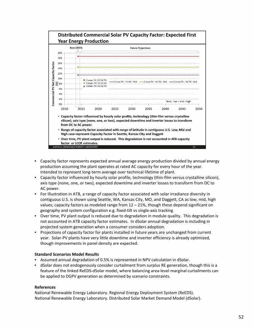
• Capacity factor represents expected annual average energy production divided by annual energy production assuming the plant operates at rated AC capacity for every hour of the year. Intended to represent long‐term average over technical lifetime of plant.
• Capacity factor influenced by hourly solar profile, technology (thin‐film versus crystalline silicon), axis type (none, one, or two), expected downtime and inverter losses to transform from DC to AC power.
• For illustration in ATB, a range of capacity factor associated with solar irradiance diversity in contiguous U.S. is shown using Seattle, WA, Kansas City, MO, and Daggett, CA as low, mid, high values; capacity factors as modeled range from 12 – 21%, though these depend significant on geography and system configuration e.g. fixed‐tilt vs single‐axis tracking
• Over time, PV plant output is reduced due to degradation in module quality. This degradation is not accounted in ATB capacity factor estimates. In dSolar annual degradation is including in projected system generation when a consumer considers adoption.
• Projections of capacity factor for plants installed in future years are unchanged from current year. Solar‐PV plants have very little downtime and inverter efficiency is already optimized,though improvements in panel density are expected.
Standard Scenarios Model Results• Assumed annual degradation of 0.5% is represented in NPV calculation in dSolar.• dSolar does not endogenously consider curtailment from surplus RE generation, though this is a
feature of the linked ReEDS‐dSolar model, where balancing area‐level marginal curtailments can be applied to DGPV generation as determined by scenario constraints.
ReferencesNational Renewable Energy Laboratory. Regional Energy Deployment System (ReEDS).National Renewable Energy Laboratory. Distributed Solar Market Demand Model (dSolar).
52

Projections of future utility‐scale PV plant CAPEX are based on the a collection of 12 system price projections from 5 separate institutions with low, mid, and high representing the minimum, median, and maximum estimates in this dataset.
Note: all prices quoted in Euros converted to USD (1 € = $1.25); all prices quoted in WAC converted to WDC (1 WAC=1.2 WDC).
Capacity factors are assumed to not increase over time. All PV system efficiency improvements are assumed to result in capital cost reductions rather than capacity factor improvements.
ReferencesUS Department of Energy, 2012. SunShot Vision Study: February 2012. NREL Report No. BK5200‐47927
Projections:
Arnulf Jäger‐Waldau, et al. (2014). ETRI 2014: Energy Technology Reference Indicator, projections for 2010‐2050. European Commission: JRC Science and Policy Reports.
Bloomberg New Energy Finance. 2015. “H2 2015 US PV Market Outlook.” November 9, 2015.
Chase, Jenny. (2015). “PV Market Outlook, Q3 2015.”Bloomberg New Energy Finance. August 17, 2015.
GTM Research. 2015. “PV Balance of Systems 2015: Technology Trends and Markets in the U.S. and Abroad.” MJ Shiao. August 2015.
International Energy Agency. (2015). World Energy Outlook 2014. February 2015.
Sharma, Ash. (2015). IHS Solar Market Intelligence. IHS. July 7, 2015.
U.S. Energy Information Administration. (2016). Annual Energy Outlook 2016 Early Release. May 2016.
53

• Note: Since the draft version of this product was posted, current and projected overnight capital cost values for the ATB mid‐case Solar PV projection have been modified downward to reflect the significant change in solar market prices that has occurred over the last year. The 2014 overnight capital cost for utility‐scale PV has been lowered to $1.90/W, a 20% reduction from the earlier draft, to be in line with the most recent quarterly solar market report available. In turn, these lower costs in 2014 have increased our confidence that the SunShot target of $1.00/W will be achieved earlier. As such, the mid‐case projection reduces the 2014 cost to $1.50/W by 2020 (same as earlier draft), and assumes the SunShot target is reached by 2030 instead of 2040 previously (reducing projected costs beyond 2020 by 10‐20% from the earlier draft).
• In general, projections represent the following trends to reduce CAPEX and FOM. The degree of adoption distinguishes between Low, Mid, and High PV Cost scenarios.
• Modules• Increased module efficiencies and increased production‐line throughput to decrease CAPEX (overhead costs
on a per‐kilowatt will go down if efficiency and throughput improvement are realized).• Reduced wafer thickness or the thickness of thin‐film semiconductor layers.• Development of new semiconductor materials.• Thin‐film (CdTE and CIGS).• Developing larger manufacturing facilities in low‐cost regions.
• Balance of System• Increased module efficiency, reducing the size of the installation.• Development of racking systems that enhance energy production or require less robust engineering.• Integration of racking or mounting components in modules.• Reduction of supply chain complexity and cost.
• Create standard packages system design.• Improve supply chains for BOS components in modules.• Create standard packaged system designs.• Improve supply chains for BOS components.
• Improved power electronics• Improve inverter prices and performance, possibly by integrating micro‐inverters.
• Decreased installation costs and margins• Reduction of supply chain margins (e.g., profit and overhead charged by suppliers, manufacturer,
distributors, and retailers); this will likely occur naturally as the U.S. PV industry grows and matures.
• Streamlining of installation practices through improved workforce development and training, and developing standardized PV hardware.
• Expansion of access to a range of innovative financing approaches and business models.• Development of best practices for permitting interconnection, and PV installation such as
subdivision regulations, new construction guidelines, and design requirements.• FOM cost reduction represents optimized O&M strategies, reduced component replacement costs and lower
frequency of component replacement.
54

55

• Solar resource prevalent throughout the U.S., but the southwest states are particularly suited to CSP plants. The resource potential for seven western states (AZ, CA, CO, NV, NM, UT, and TX) exceeds 11,000 GW assuming an annual average resource > 6.0 kWh/m2/day, and after accounting for exclusions such as land slope (>1%); urban areas; water features; and parks, preserves, andwilderness areas [Mehos, Kabel, and Smithers, 2009].
• The Solar Programmatic Environmental Impact Statement identified 17 solar energy zones (SEZ) in six western states. The 17 SEZs are priority development areas for utility‐scale solar energy facilities. These zones total 285,000 acres and are estimated to accommodate up to 24 GW of solar potential. The program also allows development, subject to a more rigorous review, on an additional 19 million acres of public land. Development is prohibited on approx. 79 million acres. [solareis.anl.gov]
• 16 of 19 currently operational CSP plants in the US using parabolic trough technology. Three power tower facilities: Ivanpah (392 MW), Crescent Dunes (110 MW), and Sierra SunTower (5 MW) are operational. Two small linear Fresnel plants are in operation. [www.nrel.gov/csp/solarpaces]
• For the ATB, 3 representative sites have been chosen based on resource class:Fair Resource e.g. Abilene Regional Airport, TX (5.59 kWh/m2/day based on the site TMY3 file)Good Resource e.g. Las Vegas, NV (7.1 kWh/m2/day based on the site TMY3 file)Excellent Resource e.g. Daggett, CA (7.46 kWh/m2/day based on the site TMY3 file)
• CAPEX determined using manufacturing cost models and benchmarked with industry data. Reflects dry‐cooling technologies to reduce water consumption.
• CF varies with inclusion of thermal energy storage. The listed projects assume Power Towers with 10hrs of thermal energy storage.
• Representative CSP plant size is net 100 MWe.
• Solar resource for the Southwest U.S. found from “CSP Today Markets Report ‐ USA”
ReferencesTurchi, C.; Kurup, P.; Akar, S.; Flores, F. (2015). “Domestic Material Content in Molten‐Salt Concentrating Solar Power Plants”. NREL, NREL Report No. TP‐5500‐64429.http://www.nrel.gov/docs/fy15osti/64429.pdf
Ballaben, S.; Poliafico, M.; Hashem, H. (2015). “CSP Today Markets Reports 2015 – USA”. CSP Today
National Renewable Energy Laboratory. (2012). Renewable Electricity Futures Study. Hand, M.M.; Baldwin, S.; DeMeo, E.; Reilly, J.M.; Mai, T.; Arent, D.; Porro, G.; Meshek, M.; Sandor, D. eds. 4 vols. NREL/TP‐6A20‐52409. Golden, CO: National Renewable Energy Laboratory. http://www.nrel.gov/analysis/re_futures/.
Mehos, M.; Kabel, D.; Smithers, P. (2009). Planting the Seed: Greening the Grid with Concentrating Solar Power. IEEE Power and Energy Magazine. Vol. 7(3), May/June 2009; pp. 55‐62; NREL Report No. JA‐550‐46134. http://dx.doi.org/10.1109/MPE.2009.932308
Bureau of Land Management and the U.S. Department of Energy. (2012). Final Programmatic Environmental Impact Statement (PEIS) for Solar Energy Development in Six Southwestern States. http://solareis.anl.gov/documents/fpeis/index.cfm.
www.nrel.gov/csp/solarpaces
56

• CAPEX in ATB represents solar CSP plant cost based on modeled system prices from industry survey plus indexed costs since last detailed cost study for the fourth quarter of the previous year.
• CAPEX in ATB may not explicitly represent regional variants associated with labor rates, material costs, etc. or geographically determined spur lines costs.• CAPEX represents total expenditure required to achieve commercial operation in a given year. Plant envelope defined to include the following based on
Beamon and Leff (2013), NREL/TP‐550‐47605, NREL/TP‐5500‐57625 • CSP Generation Plant including
• installed solar collectors, solar receiver, piping and heat‐transfer fluid system, power block (heat exchangers, power turbine, generator, cooling system), thermal energy storage system and installation
• Balance of System including• land acquisition, site preparation, installation of underground utilities, access roads, fencing, buildings for operations and
maintenance• electrical infrastructure such as transformers, switchgear and electrical system connecting modules to each other and to control
center. The generator voltage is 13.8 kV, the step‐up transformer will be 13.8/230kV, the transmission tie line will be 230 kV • project indirect costs including engineering, distributable labor and materials, construction management start up and commissioning,
and contractor overhead costs, fees and profit.• Financial Costs
• owner’s costs such as development costs, preliminary feasibility and engineering studies, environmental studies and permitting, legal fees, insurance costs, property taxes during construction
• onsite electrical equipment (e.g., switchyard), a nominal‐distance spur line (<1 mi), and necessary upgrades at a transmission substation; distance‐based spur line cost (GCC) not included in ATB.
• interest during construction estimated based on 3‐year duration accumulated 10%/10%/80% at half‐year intervals and 8% interest rate
ATB spreadsheet input is Overnight Capital Cost (OCC) and details to calculate interest during construction (ConFinFactor).
Standard Scenarios Model Results
• CAPEX in ATB does not represent regional variants (CapRegMult) associated with labor rates, material costs, etc., but ReEDS does include 134 regional multipliers (Beamon and Leff, 2013)
• CAPEX in ATB does not include geographically determined spur line (GCC) from plant to transmission grid, but ReEDS calculates a unique value for each potential CSP plant
ReferencesBeamon, A.; Leff. M. (2013). EOP III Task 1606, Subtask 3 – Review of Power Plant Cost and Performance Assumptions for NEMS. Prepared by SAIC Energy, Environment & Infrastructure, LLC for the Energy Information Administration, Office of Energy Analysis. http://www.eia.gov/forecasts/capitalcost/pdf/updated_capcost.pdf
Turchi, C. (2010). Parabolic Trough Reference Plant for Cost Modeling with the Solar Advisor Model (SAM). 112 pp.; NREL Report No. TP‐550‐47605.
Kurup, P and Turchi, C. (2015), Parabolic Trough Collector Cost Update for the System Advisor Model (SAM). NREL Report No. TP‐6A20‐65228
Turchi, C. S.; Heath, G. A. (2013). Molten Salt Power Tower Cost Model for the System Advisor Model (SAM). 53 pp.; NREL Report No. TP‐5500‐57625.
57

The CAPEX is unchanged for resource class because the same plant is assumed to be built in each location. The capacity factor will change with resource.
• Parabolic trough technology was used to describe CSP systems prior to 2025 in last year’s ATB release. For this year, it is now assumed that molten‐salt power towers are the representative technology. Either technology can incorporate TES, although power towers do that more efficiently. In both technologies, TES is accomplished by storing hot molten salt in a “2‐tank” system – a hot‐salt tank and a cold‐salt tank. Stored, hot salt can be dispatched to the power block as needed, regardless of solar conditions.
• Thermal energy storage increases plant CAPEX, but also increases CF and annual efficiency. Thermal storage lowers LCOE for power towers.
• Various US and international studies have been made, and will be continued in the future to give Historical CAPEX estimates
• For the Low Case, where Learning Rates have been applied, a Learning Rate of 9.9% for the solar field and a Learning Rate of 12% for the Turbine have been used.
• The first large Molten‐salt power tower plant (i.e. Crescent Dunes, 110MWe with 10hrs of storage) started construction in 2011, with a reported Overnight Capital Cost of $8.96/WAC
References:Kurup, P and Turchi, C. (2015), Parabolic Trough Collector Cost Update for the System Advisor Model (SAM). NREL Report No. TP‐6A20‐65228
Turchi, C. S.; Heath, G. A. (2013). Molten Salt Power Tower Cost Model for the System Advisor Model (SAM). 53 pp.; NREL Report No. TP‐5500‐57625.
Bolinger, M and Seel, J, (2015), “Utility Scale Solar 2014”, LBNL – 1000917
Rubin, E.S. et al., “A Review of Learning Rates for Electricity Supply Technologies,” Energy Policy, 86 (2015)
International Energy Agency, Technology Roadmap, Solar Thermal Electricity (2014) ‐https://www.iea.org/publications/freepublications/publication/TechnologyRoadmapSolarThermalElectricity_2014edition.pdf
Sandia National Laboratories, “Crescent Dunes Solar Energy Project”, Sandia, Jul. 2014, http://www.energystorageexchange.org/projects/348#
Mehos, M and Ho, C, (2016 ‐ in Red Team Review), “On the Path to SunShot – CSP Technology Development Roadmap”, NREL, link to be provided when released
58
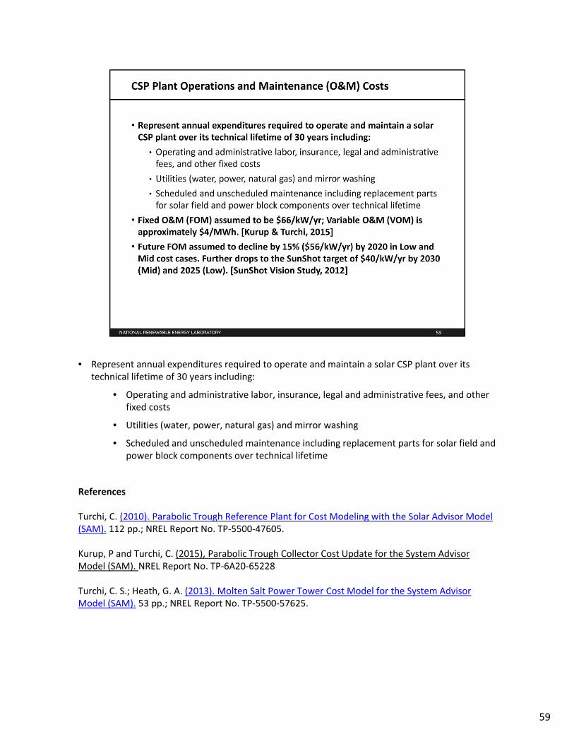
• Represent annual expenditures required to operate and maintain a solar CSP plant over its technical lifetime of 30 years including:
• Operating and administrative labor, insurance, legal and administrative fees, and other fixed costs
• Utilities (water, power, natural gas) and mirror washing
• Scheduled and unscheduled maintenance including replacement parts for solar field and power block components over technical lifetime
References
Turchi, C. (2010). Parabolic Trough Reference Plant for Cost Modeling with the Solar Advisor Model (SAM). 112 pp.; NREL Report No. TP‐5500‐47605.
Kurup, P and Turchi, C. (2015), Parabolic Trough Collector Cost Update for the System Advisor Model (SAM). NREL Report No. TP‐6A20‐65228
Turchi, C. S.; Heath, G. A. (2013). Molten Salt Power Tower Cost Model for the System Advisor Model (SAM). 53 pp.; NREL Report No. TP‐5500‐57625.
59
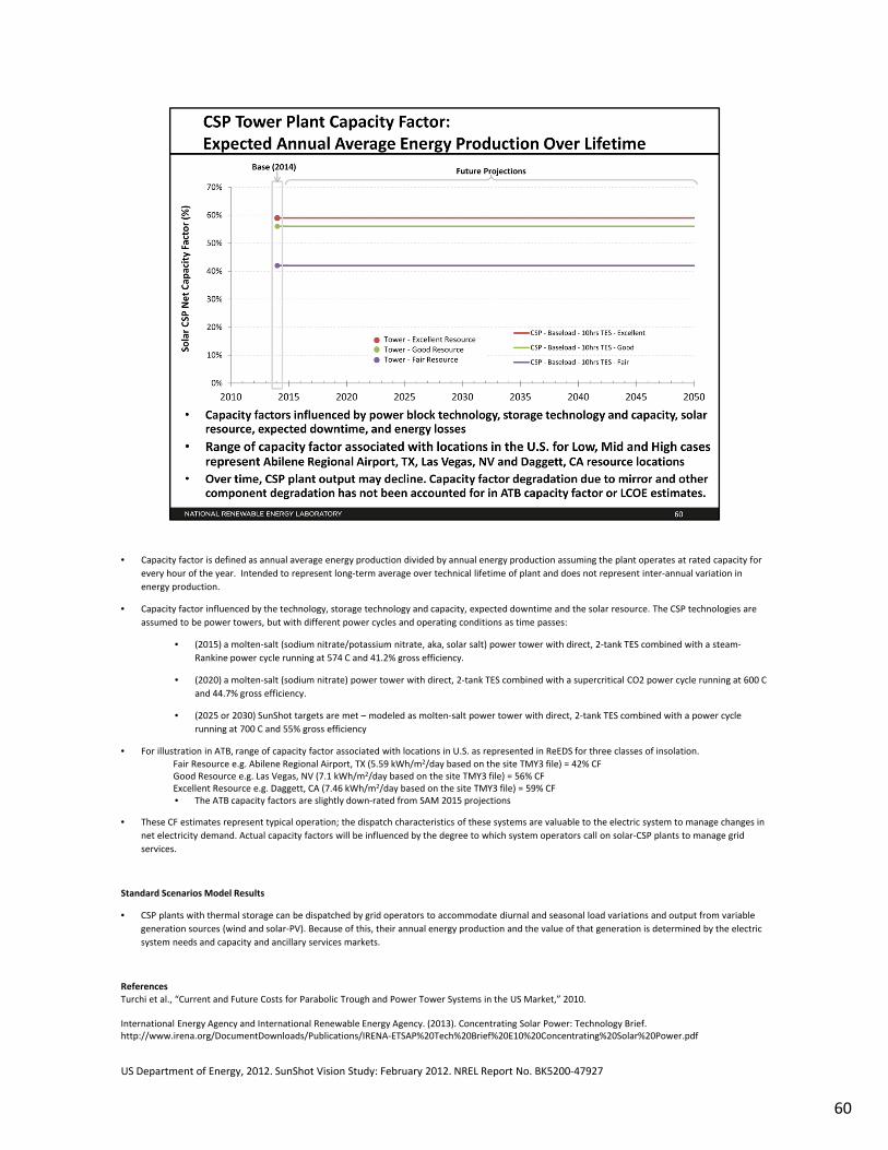
• Capacity factor is defined as annual average energy production divided by annual energy production assuming the plant operates at rated capacity for
every hour of the year. Intended to represent long‐term average over technical lifetime of plant and does not represent inter‐annual variation in
energy production.
• Capacity factor influenced by the technology, storage technology and capacity, expected downtime and the solar resource. The CSP technologies are
assumed to be power towers, but with different power cycles and operating conditions as time passes:
• (2015) a molten‐salt (sodium nitrate/potassium nitrate, aka, solar salt) power tower with direct, 2‐tank TES combined with a steam‐
Rankine power cycle running at 574 C and 41.2% gross efficiency.
• (2020) a molten‐salt (sodium nitrate) power tower with direct, 2‐tank TES combined with a supercritical CO2 power cycle running at 600 C
and 44.7% gross efficiency.
• (2025 or 2030) SunShot targets are met – modeled as molten‐salt power tower with direct, 2‐tank TES combined with a power cycle
running at 700 C and 55% gross efficiency
• For illustration in ATB, range of capacity factor associated with locations in U.S. as represented in ReEDS for three classes of insolation.
Fair Resource e.g. Abilene Regional Airport, TX (5.59 kWh/m2/day based on the site TMY3 file) = 42% CFGood Resource e.g. Las Vegas, NV (7.1 kWh/m2/day based on the site TMY3 file) = 56% CFExcellent Resource e.g. Daggett, CA (7.46 kWh/m2/day based on the site TMY3 file) = 59% CF• The ATB capacity factors are slightly down‐rated from SAM 2015 projections
• These CF estimates represent typical operation; the dispatch characteristics of these systems are valuable to the electric system to manage changes in
net electricity demand. Actual capacity factors will be influenced by the degree to which system operators call on solar‐CSP plants to manage grid
services.
Standard Scenarios Model Results
• CSP plants with thermal storage can be dispatched by grid operators to accommodate diurnal and seasonal load variations and output from variable
generation sources (wind and solar‐PV). Because of this, their annual energy production and the value of that generation is determined by the electric
system needs and capacity and ancillary services markets.
References
Turchi et al., “Current and Future Costs for Parabolic Trough and Power Tower Systems in the US Market,” 2010.
International Energy Agency and International Renewable Energy Agency. (2013). Concentrating Solar Power: Technology Brief. http://www.irena.org/DocumentDownloads/Publications/IRENA‐ETSAP%20Tech%20Brief%20E10%20Concentrating%20Solar%20Power.pdf
US Department of Energy, 2012. SunShot Vision Study: February 2012. NREL Report No. BK5200‐47927
60

• Projections based on SunShot Vision study and vetted with solar industry participants.
• Attempts have been made to clarify the specifics (e.g. number of hours of storage, solar multiple) of the other published CSPprojections. As yet, this has not been possible
• Three different projections developed for scenario modeling as bounding levels
• (High) – Molten‐salt (sodium nitrate/potassium nitrate, aka, solar salt) power tower with direct, 2‐tank TES combined with a steam‐Rankine power
cycle running at 574 C and 41.2% gross efficiency in 2015. Costs stay same over time
• (Mid) ‐ A molten‐salt (sodium nitrate) power tower with direct, 2‐tank TES combined with a supercritical CO2 power cycle running at 600 C and
44.7% gross efficiency in 2020. SunShot targets are met in 2030 – modeled as molten‐salt power tower with direct, 2‐tank TES combined with a
power cycle running at 700 C and 55% gross efficiency.
• (Low) SunShot targets are met in 2025 – modeled as molten‐salt power tower with direct, 2‐tank TES combined with a power cycle running at 700 C
and 55% gross efficiency. For the Low Case, where Learning Rates have been applied, a Learning Rate of 9.9% for the solar field and a Learning Rate
of 12% for the Turbine have been used.
ReferencesUS Department of Energy, 2012. SunShot Vision Study: February 2012. NREL Report No. BK5200‐47927
Sandia National Laboratory. (2011). Power Tower Technology Roadmap. SAND2011‐2419.
International Renewable Energy Agency. (2012). Renewable Energy Technologies: Cost Analysis Series, Concentrating Solar Power. http://costing.irena.org/media/2794/re_technologies_cost_analysis‐csp.pdf
Lazard. (2014). Lazard’s Levelized Cost of Energy Analysis – Version 8.0. http://www.lazard.com/PDF/Levelized%20Cost%20of%20Energy%20‐%20Version%208.0.pdf
Ash, K.; Teske, S.; Sawyer, S.; Schafer, O. (2015). Energy [r]evolution: A Sustainable World Energy Outlook 2015. Global Wind Energy Council, Solar Power Europe & Greenpeace. September 2015
Arnulf Jäger‐Waldau, et al. (2014). ETRI 2014: Energy Technology Reference Indicator, projections for 2010‐2050. European Commission: JRC Science and Policy Reports.
International Energy Agency. (2015). World Energy Outlook 2015. November 2015.
Mills, Luke. (2015). H2 2015 Global Levelized Cost Of Electricity Update. Bloomberg New Energy Finance. October 1, 2015.
U.S. Energy Information Administration. (2016). Annual Energy Outlook 2016 Early Release. May 2016.
61

In general, projections represent the following trends, and the degree of adoption distinguishes between Low, Mid and High CSP Cost scenarios as described on previous slide.
LCOE range shown based on locations with Fair, Good and Excellent resources. The CAPEX is the same at each resource as the same plant is used
Resources taken at i.e. Fair ‐ Abilene Regional Airport, TX; Good ‐ Las Vegas, NV; and Excellent ‐Daggett, CA.
Power Tower improvements:• Better and longer‐lasting selective surface coatings improve receiver efficiency and reduce O&M
costs• New salts allow for higher operating temperatures and lower cost TES• Development of the supercritical CO2 power cycle improves cycle efficiency, reduces
powerblock cost, and reduces O&M costs• Lower cost heliostats developed due to more efficient designs, and automated and high‐volume
manufacturing
General and “soft” costs improvements:• Modular plant designs decrease installation costs and margins• Expansion of world market leads to greater and more efficient supply chains; reduction of supply
chain margins (e.g., profit and overhead charged by suppliers, manufacturer, distributors, and retailers)
• Expansion of access to a range of innovative financing approaches and business models• Development of best practices for permitting interconnection, and installation such as
subdivision regulations, new construction guidelines, and design requirements
62

63

• Hydrothermal geothermal resource concentrated in Western US – total potential is 45,370 MW• Identified Hydrothermal from USGS 2008 Updated Geothermal Resource Assessment
• Resource potential estimate at each site identified by USGS based on available reservoir thermal energy information from studies conducted at the site.
• Installed capacity of about 3 GW in 2014 excluded from resource potential• Resource potential estimates increased 20‐30% to reflect impact of in‐field EGS technologies to
increase productivity of dry wells and increase recovery of heat in place from hydrothermal reservoirs.
• Undiscovered hydrothermal values from USGS 2008 Updated Geothermal Resource Assessment • Resource potential estimated based on a series of GIS statistical models for the spatial
correlation of geological factors that facilitate the formation of geothermal systems.• Resource potential estimates increased 20‐30% to reflect impact of in‐field EGS technologies to
increase productivity of dry wells and increase recovery of heat in place from hydrothermal reservoirs.
• Hydrothermal generation plant cost and performance estimated for each potential site using GETEM, a bottom‐up cost analysis tool that accounts for each phase of development of a geothermal plant. Model results based on resource attributes (estimated reservoir temperature, depth, and potential) at each site.
• Site attribute values from USGS (2008) for identified resource potential, and capacity weighted averages of site attribute values from nearby identified resources for undiscovered resource potential.
• GETEM used to estimate overnight capital cost, and parasitic plant losses that affect net energy production
• Typical geothermal plant size for hydrothermal resource sites are represented from 30 MW to 40 MW depending on technology type, binary or flash. https://www4.eere.energy.gov/geothermal/sites/default/files/documents/mines_getem_peer2013.pdf, Slide 9.
ReferencesU .S. Department of Energy. (2012). Geothermal Energy Technology Evaluation Model (GETEM). http://energy.gov/eere/geothermal/geothermal‐electricity‐technology‐evaluation‐model.
Williams, C.; Reed, M.; Mariner, R.; DeAngelo, J.; Galanis, S. (2008). Assessment of moderate‐ and high‐temperature geothermal resources of the United States: U.S. Geological Survey Fact Sheet 2008‐3082.
64

• Near Field‐EGS Resource Potential based on data from USGS for EGS potential on the periphery of select, studied, identified hydrothermal sites estimated at 1,493 MW.
• Deep EGS resource potential (Augustine 2011), based on SMU Geothermal Laboratory temp‐at‐depth maps and methodology from MIT Future of Geothermal Energy Report
• EGS resource is thousands of GW (16,000 GW) and many locations are likely not commercially feasible.
• Approaches to restrict resource potential to about 500 GW based on USGS analysis may be implemented in the future.
• EGS generation plant cost and performance estimated for each potential site using GETEM, a bottom‐up cost analysis tool that accounts for each phase of development of a geothermal plant. Model results based on resource attributes (estimated reservoir temperature, depth, and potential) at each site.
• Site attribute values from USGS (2008) for identified resource potential, and capacity weighted averages of site attribute values from nearby identified resources for undiscovered resource potential.
• GETEM used to estimate overnight capital cost, and parasitic plant losses that affect net energy production
• Typical geothermal plant size for enhanced geothermal system plants are represented by a range from 20 MW to 25 MW for binary or flash technologies. https://www4.eere.energy.gov/geothermal/sites/default/files/documents/mines_getem_peer2013.pdf, Slide 9.
ReferencesAugustine, C. (2011). Updated U.S. Geothermal Supply Characterization and Representation for Market Penetration Model Input. 103 pp.; NREL Report No. TP‐6A2‐47459.
Robert, B. (2009). Geothermal Resource of the United States: Locations of Identified Hydrothermal Sites and Favorability of Deep Enhanced Geothermal Systems (EBS). National Renewable Energy Laboratory. http://www.nrel.gov/gis/pdfs/National%20Geothermal%20EGS%20Hydrothermal%20%202009.pdf
U.S. Department of Energy. (2012). Geothermal Energy Technology Evaluation Model (GETEM). http://energy.gov/sites/prod/files/2014/02/f7/geothermal_electricity_technology_evaluation_model_may_2011.pdf
Williams, C.; Reed, M.; Mariner, R.; DeAngelo, J.; Galanis, S. (2008). Assessment of moderate‐ and high‐temperature geothermal resources of the United States: U.S. Geological Survey Fact Sheet 2008‐3082.
65

• CAPEX in ATB based on GETEM model results using resource attributes (estimated reservoir temperature, depth, and potential) at each site.
• CAPEX in ATB does not explicitly represent regional variants associated with labor rates, material costs, etc. or geographically determined spur line costs.
• CAPEX represents total expenditure required to achieve commercial operation in a given year. Plant envelope defined to include the following based on GETEM component cost calculations and (Beamon and Leff, 2013):
• Geothermal Generation Plant including• exploration (including exploration at “unsuccessful” sites), confirmation drilling, well field development,
reservoir stimulation (EGS), and plant construction• power plant equipment, well‐field equipment and components for wells (including dry/non‐commercial
wells)• Balance of System including
• electrical infrastructure such as transformers, switchgear and electrical system connecting turbines to each other and to control center
• project indirect costs including engineering, distributable labor and materials, construction management start up and commissioning, and contractor overhead costs, fees and profit.
• Financial Costs• owner’s costs such as development costs, preliminary feasibility and engineering studies, environmental
studies and permitting, legal fees, insurance costs, property taxes during construction• onsite electrical equipment (e.g., switchyard), a nominal‐distance spur line (<1 mi), and necessary upgrades at
a transmission substation; distance‐based spur line cost (GCC) not included in ATB. • interest during construction estimated based on 3‐year duration accumulated 10%/10%/80% at half‐year
intervals and 8% interest rate• ATB spreadsheet input is Overnight Capital Cost (OCC) and details to calculate interest during
construction (ConFinFactor).
Standard Scenarios Model Results• CAPEX in ATB does not represent regional variants (CapRegMult) associated with labor rates, material costs, etc., and neither does
ReEDS• CAPEX in ATB does not include geographically determined spur line (GCC) from plant to transmission grid, and neither does ReEDS
ReferencesBeamon, A.; Leff. M. (2013). EOP III Task 1606, Subtask 3 – Review of Power Plant Cost and Performance Assumptions for NEMS. Prepared by SAIC Energy, Environment & Infrastructure, LLC for the Energy Information Administration, Office of Energy Analysis.http://www.eia.gov/forecasts/capitalcost/pdf/updated_capcost.pdf
Mines, G.; and Nathwani, J. (2013). Estimated Power Generation Costs for EGS. Proceedings for the Thirty‐Eight Workshop on Geothermal Reservoir Engineering. Stanford University, Stanford, California, February 11‐13, 2013. Idaho National Laboratory and the U.S. Department of Energy.http://www.geothermal‐energy.org/pdf/IGAstandard/SGW/2013/Nathwani.pdf?
U.S. Department of Energy (2014). “GETEM Development.” U.S. Department of Energy website. http://www4.eere.energy.gov/geothermal/projects/1096.
U.S. Department of Energy. (2012). Geothermal Energy Technology Evaluation Model (GETEM). http://energy.gov/eere/geothermal/geothermal‐electricity‐technology‐evaluation‐model
66

• For illustration in ATB, six representative geothermal plants are shown. Two energy conversion processes are common: binary organic Rankine cycle and flash. Examples using each of these plant types in each of the three resource types, hydrothermal (hydro), near‐hydrothermal field EGS (NF‐EGS) and deep EGS, are shown.
• Costs are for new or “greenfield” hydrothermal projects, not for re‐drilling or additional development/capacity additions at an existing site.• Binary organic Rankine cycle plants use a heat exchanger to transfer geothermal energy to the steam turbine generator; this technology generally applies to lower temperature
systems. Due to the increased number of components, lower temperature operation, and general requirement for a number of wells to be drilled for a given power output, these systems have higher CAPEX than flash systems.
• Flash plants create steam directly from the thermal fluid through a pressure change; this technology generally applies to higher temperature systems. Due to the reduced number of components, higher temperature operation, these systems generally produce more power per well reducing drilling costs. These systems generally have lower CAPEX than binary systems.
• Characteristics for the six example plants representing current technology were developed based on discussion with industry stakeholders (GTO internal). The CAPEX estimates were estimated using GETEM. CAPEX for NF‐EGS and EGS are equivalent. The table below shows the range of OCC associated with the resource characteristics for potential sites throughout the U.S.
• Projection of future geothermal plant CAPEX is based on minimum learning rates as implemented in AEO 2015, 10% by 2035 and extrapolated to 2050.
Standard Scenario Model Results• ReEDS represents cost and performance for hydrothermal, NF‐EGS and EGS potential in five bins for each of 134 geographic regions resulting in greater CAPEX range in the
reference supply curve than what is shown in examples in ATB.
Future ATB Representation Under Consideration• For this version of the ATB, future geothermal CAPEX are assumed to be the same as current costs. It is anticipated that ongoing GTO‐directed analysis will improve this
assumption for future versions of the ATB.
References• Mines, G.; Nathwani, J. (2013). Geothermal Electricity Technology Evaluation Model. U.S. Department of Energy, Geothermal Technologies Office 2013 Peer Review
Http://www4.eere.energy.gov/geothermal/sites/default/files/documents/mines_getem_peer2013.pdf• EIA (2015). Annual Energy Outlook.
67

• Represent average annual fixed expenditures (depend on rated capacity) required to operate and maintain a hydropower plant over its technical lifetime (plant and reservoir) of 30 years including:
• Insurance, taxes, land lease payments, and other fixed costs• Present value, annualized large component overhaul or replacement costs over
technical life (e.g. downhole pumps)• Scheduled and unscheduled maintenance of geothermal plant components and well
field components over plant and reservoir technical lifetime• GETEM used to estimate FOM for each of six representative plants. Characteristics for the six
example plants representing current technology were developed based on discussion with industry stakeholders (GTO internal). FOM for NF‐EGS and EGS are equivalent.
• No future FOM cost reduction assumed in this edition of ATB
Standard Scenarios Model Results• ReEDS Version 2016.1 standard scenario model results use FOM from AEO 2014 for all
geothermal resource types and technologies.
ReferencesU.S. Department of Energy. (2012). Geothermal Energy Technology Evaluation Model (GETEM). http://energy.gov/sites/prod/files/2014/02/f7/geothermal_electricity_technology_evaluation_model_may_2011.pdf
U.S. Energy Information Administration, U.S. Department of Energy (EIA). (2014a). Annual Energy Outlook 2014 with Projections to 2040. DOE/EIA‐0383(2014). Washington, D.C.: U.S. Department of Energy Office of Integrated and International Energy Analysis. http://www.eia.gov/forecasts/aeo/pdf/0383(2014).pdf
68

• Capacity factor represents expected annual average energy production divided by annual energy production assuming the plant operates at rated capacity for every hour of the year. Intended to represent long‐term average over technical lifetime of plant and does not represent inter‐annual variation in energy production.
• Capacity factor influenced by diurnal and seasonal air temperature variation (for air‐cooled plants), technology (binary, flash, etc.), downtime and internal plant energy losses.
• Capacity factor estimates developed using GETEM at typical design air temperature and based on design plant capacity net losses. Additional reduction applied to approximate potential variability due to seasonal temperature effects.
• Some geothermal plants have experienced year‐on‐year reductions in energy production, but this is not consistent across all plants. No approximation of long‐term degradation of energy output is assumed.
• Ongoing work at NREL and INL is helping to improve capacity factor estimates for geothermal plants. As their work progresses, it will be incorporated into future versions of the ATB.
ReferencesU.S. Department of Energy. (2012). Geothermal Energy Technology Evaluation Model (GETEM). http://energy.gov/sites/prod/files/2014/02/f7/geothermal_electricity_technology_evaluation_model_may_2011.pdf
69
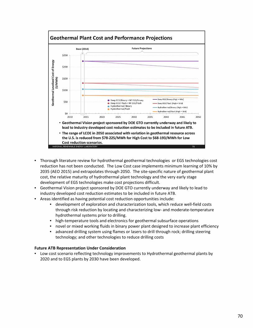
• Thorough literature review for hydrothermal geothermal technologies or EGS technologies cost reduction has not been conducted. The Low Cost case implements minimum learning of 10% by 2035 (AEO 2015) and extrapolates through 2050. The site‐specific nature of geothermal plant cost, the relative maturity of hydrothermal plant technology and the very early stage development of EGS technologies make cost projections difficult.
• Geothermal Vision project sponsored by DOE GTO currently underway and likely to lead to industry developed cost reduction estimates to be included in future ATB.
• Areas identified as having potential cost reduction opportunities include:• development of exploration and characterization tools, which reduce well‐field costs
through risk reduction by locating and characterizing low‐ and moderate‐temperature hydrothermal systems prior to drilling.
• high‐temperature tools and electronics for geothermal subsurface operations• novel or mixed working fluids in binary power plant designed to increase plant efficiency• advanced drilling system using flames or lasers to drill through rock; drilling steering
technology; and other technologies to reduce drilling costs
Future ATB Representation Under Consideration• Low cost scenario reflecting technology improvements to Hydrothermal geothermal plants by
2020 and to EGS plants by 2030 have been developed.
70

Note: pumped storage hydropower is considered a storage technology in ATB and will be addressed in future years. Pumped storage hydropower, and other storage technologies, are represented in Standard Scenarios Model Results from ReEDS model.
71
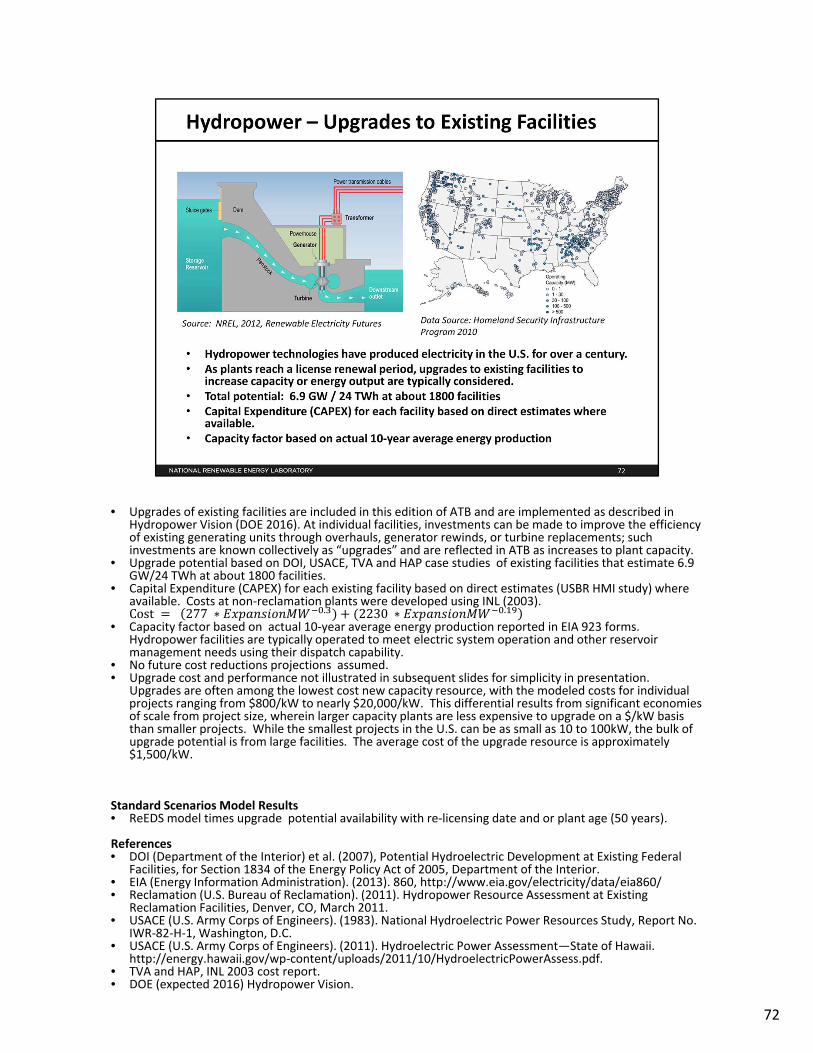
• Upgrades of existing facilities are included in this edition of ATB and are implemented as described in Hydropower Vision (DOE 2016). At individual facilities, investments can be made to improve the efficiency of existing generating units through overhauls, generator rewinds, or turbine replacements; such investments are known collectively as “upgrades” and are reflected in ATB as increases to plant capacity.
• Upgrade potential based on DOI, USACE, TVA and HAP case studies of existing facilities that estimate 6.9 GW/24 TWh at about 1800 facilities.
• Capital Expenditure (CAPEX) for each existing facility based on direct estimates (USBR HMI study) where available. Costs at non‐reclamation plants were developed using INL (2003). Cost 277 ∗ . 2230 ∗ .
• Capacity factor based on actual 10‐year average energy production reported in EIA 923 forms. Hydropower facilities are typically operated to meet electric system operation and other reservoir management needs using their dispatch capability.
• No future cost reductions projections assumed.• Upgrade cost and performance not illustrated in subsequent slides for simplicity in presentation.
Upgrades are often among the lowest cost new capacity resource, with the modeled costs for individual projects ranging from $800/kW to nearly $20,000/kW. This differential results from significant economies of scale from project size, wherein larger capacity plants are less expensive to upgrade on a $/kW basis than smaller projects. While the smallest projects in the U.S. can be as small as 10 to 100kW, the bulk of upgrade potential is from large facilities. The average cost of the upgrade resource is approximately $1,500/kW.
Standard Scenarios Model Results• ReEDS model times upgrade potential availability with re‐licensing date and or plant age (50 years).
References• DOI (Department of the Interior) et al. (2007), Potential Hydroelectric Development at Existing Federal
Facilities, for Section 1834 of the Energy Policy Act of 2005, Department of the Interior.• EIA (Energy Information Administration). (2013). 860, http://www.eia.gov/electricity/data/eia860/• Reclamation (U.S. Bureau of Reclamation). (2011). Hydropower Resource Assessment at Existing
Reclamation Facilities, Denver, CO, March 2011.• USACE (U.S. Army Corps of Engineers). (1983). National Hydroelectric Power Resources Study, Report No.
IWR‐82‐H‐1, Washington, D.C.• USACE (U.S. Army Corps of Engineers). (2011). Hydroelectric Power Assessment—State of Hawaii.
http://energy.hawaii.gov/wp‐content/uploads/2011/10/HydroelectricPowerAssess.pdf.• TVA and HAP, INL 2003 cost report.• DOE (expected 2016) Hydropower Vision.
72

• Nationally, more than 80,000 dams exist which do not produce power. This dataset from the National Inventory of Dams (NID) was filtered to remove dams with erroneous flow and geographic data, or dams whose data could not be resolved to a satisfactory level of detail (Hadjerioua, et al., 2012). This initial assessment of 54,391 dams resulted in 12 GW of capacity.
• A new methodology for sizing potential hydropower facilities that was developed for the New‐Stream Reach Development resource (Kao et al., 2014) was applied to non‐powered dams. Final resource potential estimated to be 5.9 GW / 33 TWh at over 54,000 dams. This method is summarized below.
• About 600 existing facilities were evaluated to assess resource potential (capacity) and energy generation potential (CF). For each facility a design capacity, average monthly flow rate over a 20‐year period and design flow rate exceedance level of 30% are assumed. The exceedance level represents the fraction of time that the design flow is exceeded. This parameter can be varied and results in different capacity and energy generation for a given site. The value of 30% was chosen based on industry rules of thumb. The capacity factor for a given facility is determined by these design criteria.
• CAPEX for each facility is based on statistical analysis of historic plant data from 1980 to 2015 as a function of key design parameters, plant capacity and hydraulic head (O’Connor et al., 2015).
• Cost 11,489,245 ∗ . ∗ . 310,000 ∗.
Standard Scenarios Model Results• ReEDS Version 2016.1 standard scenario model results restrict the resource potential to sites greater than 500 kW
resulting in 5.1 GW / 28 TWh at 667 dams.
ReferencesHadjerioua, B. et al. (2012). An Assessment of Energy Potential at Non‐Powered Dams in the United States. Prepared by Oakridge National Laboratory for the U.S. Department of Energy. http://www1.eere.energy.gov/water/pdfs/npd_report.pdf
Hall et al. (2003). Estimation of Economic Parameters of U.S. Hydropower Resources. Idaho National Laboratory. http://www1.eere.energy.gov/water/pdfs/doewater‐00662.pdf.
Kao et al. (2014). New Stream‐reach Development: A Comprehensive Assessment of Hydropower Energy Potential in the United States. Prepared by Oakridge National Laboratory for the U.S. Department of Energy. New Stream‐reach Development: A Comprehensive Assessment of Hydropower Energy Potential in the United States
O’Connor, P.W., S.T. DeNeale, D.R. Chalise, A. Maloof (2015). Hydropower Baseline Cost Modeling, Version 2. ORNL/TM‐2015/471. Oak Ridge, TN: Oak Ridge National Laboratory.
Oakridge National Laboratory. Hydropower Resource Map expected publication 2015.
73

• Resource potential estimated to be 53.2 GW / 301 TWh at nearly 230,000 individual sites (Kao et al., 2014) after accounting for exclusions such as national parks, wild and scenic rivers, and wilderness areas.
• About 8500 stream reaches were evaluated to assess resource potential (capacity) and energy generation potential (CF). For each stream reach a design capacity, average monthly flow rate over 20‐year period and design flow rate exceedance level of 30% are assumed. The exceedance level represents the fraction of time that the design flow is exceeded. This parameter can be varied and results in different capacity and energy generation for a given site. The value of 30% was chosen based on industry rules of thumb. The capacity factor for a given facility is determined by these design criteria. Plant sizes range from kW to multi‐MW (Kao et al., 2014).
• Resource assessment approach designed to minimize footprint of hydropower facility by restricting inundation area to FEMA 100 year flood plain.
• New hydropower facilities are assumed to apply run of river operation strategies. Run of river operation means that flow rate into reservoir is equal to flow rate out of facility. These facilities do not have dispatch capability.
• CAPEX for each facility is based on statistical analysis of historic plant data from 1980 to 2015 as a function of key design parameters, plant capacity and hydraulic head (O’Connor et al., 2015).
• Cost 9,605,710 ∗ . ∗ . 610,000 ∗.
Standard Scenarios Model Results• ReEDS Version 2016.1 standard scenario model results restrict the resource potential to sites greater than
1 MW resulting in 30.1 GW / 176 TWh at nearly 8000 sites.
References• Kao et al. (2014). New Stream‐reach Development: A Comprehensive Assessment of Hydropower Energy
Potential in the United States. Prepared by Oakridge National Laboratory for the U.S. Department of Energy. New Stream‐reach Development: A Comprehensive Assessment of Hydropower Energy Potential in the United States
• O’Connor, P.W., S.T. DeNeale, D.R. Chalise, A. Maloof (2015). Hydropower Baseline Cost Modeling, Version 2. ORNL/TM‐2015/471. Oak Ridge, TN: Oak Ridge National Laboratory.
74
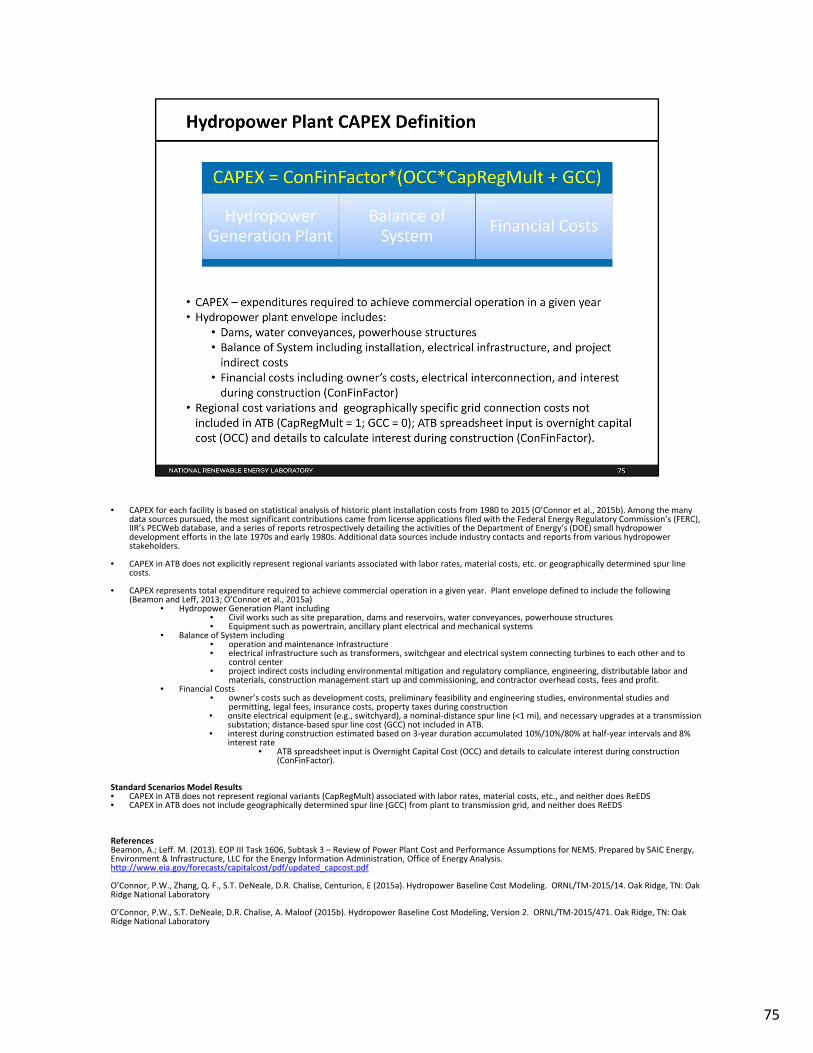
• CAPEX for each facility is based on statistical analysis of historic plant installation costs from 1980 to 2015 (O’Connor et al., 2015b). Among the many data sources pursued, the most significant contributions came from license applications filed with the Federal Energy Regulatory Commission’s (FERC), IIR’s PECWeb database, and a series of reports retrospectively detailing the activities of the Department of Energy’s (DOE) small hydropower development efforts in the late 1970s and early 1980s. Additional data sources include industry contacts and reports from various hydropower stakeholders.
• CAPEX in ATB does not explicitly represent regional variants associated with labor rates, material costs, etc. or geographically determined spur line costs.
• CAPEX represents total expenditure required to achieve commercial operation in a given year. Plant envelope defined to include the following (Beamon and Leff, 2013; O’Connor et al., 2015a)
• Hydropower Generation Plant including• Civil works such as site preparation, dams and reservoirs, water conveyances, powerhouse structures• Equipment such as powertrain, ancillary plant electrical and mechanical systems
• Balance of System including• operation and maintenance infrastructure• electrical infrastructure such as transformers, switchgear and electrical system connecting turbines to each other and to
control center• project indirect costs including environmental mitigation and regulatory compliance, engineering, distributable labor and
materials, construction management start up and commissioning, and contractor overhead costs, fees and profit.• Financial Costs
• owner’s costs such as development costs, preliminary feasibility and engineering studies, environmental studies and permitting, legal fees, insurance costs, property taxes during construction
• onsite electrical equipment (e.g., switchyard), a nominal‐distance spur line (<1 mi), and necessary upgrades at a transmission substation; distance‐based spur line cost (GCC) not included in ATB.
• interest during construction estimated based on 3‐year duration accumulated 10%/10%/80% at half‐year intervals and 8% interest rate
• ATB spreadsheet input is Overnight Capital Cost (OCC) and details to calculate interest during construction (ConFinFactor).
Standard Scenarios Model Results• CAPEX in ATB does not represent regional variants (CapRegMult) associated with labor rates, material costs, etc., and neither does ReEDS• CAPEX in ATB does not include geographically determined spur line (GCC) from plant to transmission grid, and neither does ReEDS
ReferencesBeamon, A.; Leff. M. (2013). EOP III Task 1606, Subtask 3 – Review of Power Plant Cost and Performance Assumptions for NEMS. Prepared by SAIC Energy, Environment & Infrastructure, LLC for the Energy Information Administration, Office of Energy Analysis. http://www.eia.gov/forecasts/capitalcost/pdf/updated_capcost.pdf
O’Connor, P.W., Zhang, Q. F., S.T. DeNeale, D.R. Chalise, Centurion, E (2015a). Hydropower Baseline Cost Modeling. ORNL/TM‐2015/14. Oak Ridge, TN: Oak Ridge National Laboratory
O’Connor, P.W., S.T. DeNeale, D.R. Chalise, A. Maloof (2015b). Hydropower Baseline Cost Modeling, Version 2. ORNL/TM‐2015/471. Oak Ridge, TN: Oak Ridge National Laboratory
75

• For illustration in ATB, all potential NPD and NSD sites were first binned by both head and capacity. Analysis of these bins provided groupings that represented the most realistic conditions for future hydropower deployment. The design values of these four reference NPD and four reference NSDplants are shown below. The full range of resource and design characteristics are in the ATB spreadsheet.
• The reference plants shown below were developed using the average characteristics (weighted by capacity) of the resource plants within each set of ranges. For example, NPD 1 is constructed from the capacity‐weighted average values of NPD sites between 3‐30 feet of head and 0.5‐10 MW of capacity.
• The weighted average values were used as input to the cost formulas (O’Connor et al., 2015) in order to calculate site CAPEX and O&M costs.
• Actual and proposed NPD and NSD CAPEX from 1981‐2014 (from O’Connor et al. 2015) are shown in box and whiskers format (bar represents median, box represents 25th and 75th percentile, whiskers represent minimum and maximum; diamond represents capacity weighted average) for comparison to ATB current CAPEX estimates and future projections.
• NPD CAPEX ATB estimates range from $3,700/kW to nearly $6,000/kW; the higher cost sites generally reflect very smaller capacity (<10 MW), low head sites which have fewer analogues in the historical data, but these characteristics result in higher CAPEX.
• NSD CAPEX in ATB ranges from $5,500/kW to $6,900/kW; in general, NSD potential represents smaller capacity facilities with lower head than most historical data represents. These characteristics lead to higher CAPEX estimates than past data suggests.
Standard Scenarios Model Results• ReEDS Version 2015.1 standard scenario model results use resource/cost supply curves representing estimates at each individual facility (~700 NPD,
~8000 NSD).• ReEDS represents cost and performance for NPD and NSD potential in five bins for each of 134 geographic regions resulting in CAPEX range from
$2300/kW to $66,000/kW for NPD resource and from $5500/kW to $13,000/kW for NSD.• ReEDS represents cost and performance for NPD and NSD potential in five bins for each of 134 geographic regions resulting in CF range from 38% to
80% for NPD resource and from 53% to 81% for NSD.
References• O’Connor, P.W., S.T. DeNeale, D.R. Chalise, A. Maloof (2015). Hydropower Baseline Cost Modeling, Version 2. ORNL/TM‐2015/471. Oak Ridge, TN: Oak
Ridge National Laboratory.
76
Plants Head (feet) Capacity (MW) Head (feet) Capacity (MW) Capacity Factor ICC (2014$/kW) O&M (2014$/kW)
NPD 1 3‐30 0.5‐10 15.4 4.8 0.62 5,937.86$ 111.14$
NPD 2 3‐30 10+ 15.9 82.2 0.64 5,404.59$ 30.58$
NPD 3 30+ 0.5‐10 89.6 4.2 0.60 3,976.71$ 118.05$
NPD 4 30+ 10+ 81.3 44.7 0.60 3,749.35$ 40.32$
NSD 1 3‐30 1‐10 15.7 3.7 0.66 6,997.72$ 124.36$
NSD 2 3‐30 10+ 19.6 44.1 0.66 6,247.04$ 40.55$
NSD 3 30+ 1‐10 46.8 4.3 0.62 6,118.62$ 116.99$
NSD 4 30+ 10+ 45.3 94.0 0.66 5,508.15$ 28.78$
Resource Characteristics Ranges Weighted Average Values Calculated Plant Values

• Represent average annual fixed expenditures (depend on rated capacity) required to operate and maintain a hydropower plant over its technical lifetime of 50 years including:
• Insurance, taxes, land lease payments, and other fixed costs• Present value, annualized large component overhaul or replacement costs over
technical life (e.g. rewind stator, patch cavitation damage, replace bearings)• Scheduled and unscheduled maintenance of hydropower plant components including
turbines, generators, etc. over technical lifetime• Statistical analysis of long‐term plant operation costs from FERC Form‐1 resulted in a
relationship between annual, fixed O&M costs and plant capacity (O’Connor et al., 2015).
• & 2014$ 225,417 . 2.5%
• O&M costs for reference NPD and NSD plants shown earlier.• No future FOM cost reduction assumed in this edition of ATB.
References• O’Connor, P.W., S.T. DeNeale, D.R. Chalise, A. Maloof (2015). Hydropower Baseline Cost
Modeling, Version 2. ORNL/TM‐2015/471. Oak Ridge, TN: Oak Ridge National Laboratory.
77

• Capacity factor represents expected annual average energy production divided by annual energy production assuming the plant operates at rated capacity for every hour of the year. Intended to represent long‐term average over technical lifetime of plant and does not represent inter‐annual variation in energy production.
• Capacity factor influenced by site hydrology, design factors (e.g., exceedance level) and operation characteristics (dispatch or run of river). Capacity factor for all potential NPD sites and NSD stream reaches estimated based on design criteria, long‐term monthly flow rate records and run of river operation.
• For illustration in ATB, all potential NPD and NSD sites were represented with four reference plant each as described on an earlier slide.
• Actual energy production from about 200 run of river plants operating in the U.S. from 2003 to 2012 (EIA) is shown in box and whiskers format for comparison with current estimates and future projections. This sample includes some very old plants that may have lower availability and efficiency losses. It also includes plants that have been relicensed and may no longer be optimally designed for current operating regime (e.g., a peaking unit now operating as run of river). This contributes to the broad range, particularly on the low end.
• Current and future estimates for new hydropower plants are within the range of observed plant performance. These potential new hydropower plants would be designed for specific site conditions which would indicate operation toward the high end of the range.
• Inter‐annual variation of hydropower plant output for run of river plants may be significant due to hydrological changes such as drought. This impact may be exacerbated by climate change over the long term.
Standard Scenarios Model Results• ReEDS Version 2016.1 standard scenario model results use resource/cost supply curves representing estimates at
each individual facility (~700 NPD, ~8000 NSD).• ReEDS represents cost and performance for NPD and NSD potential in five bins for each of 134 geographic regions
resulting in CF range from 38% to 80% for NPD resource and from 53% to 81% for NSD.• Existing hydropower facilities in ReEDS provide dispatch capability such that their annual energy production is
determined by the electric system needs by dispatching generators to accommodate diurnal and seasonal load variations and output from variable generation sources (wind and solar‐PV).
References• EIA data for historic capacity factor• Kao et al. (2014). New Stream‐reach Development: A Comprehensive Assessment of Hydropower Energy Potential in
the United States. Prepared by Oakridge National Laboratory for the U.S. Department of Energy. New Stream‐reach Development: A Comprehensive Assessment of Hydropower Energy Potential in the United States
78

• A range of future cost outcomes was developed for the DOE Hydropower Vision (expected 2016) study using bottom‐up analysis of process and/or technology improvements. The Mid and Low cost cases use a mix of inputs based on U.S. Energy Information Administration (EIA) technological learning assumptions, input from a technical team of Oak Ridge National Laboratory (ORNL) researchers, and the experience of expert hydropower consultants. Estimated 2035 cost levels are intended to provide magnitude of order cost reductions deemed to be at least conceptually possible and are meant to stimulate a broader discussion with the hydropower industry and its stakeholders that will be necessary to the future of cost reduction in the hydropower industry. Cost projections were derived independently for NPD and NSD technologies.
• ATB cost projections are compared to published literature for context. Published literature represents 7 independent published studies and 11 different cost projection scenarios within these studies. Cost reduction literature for hydropower is limited with several studies projecting no change through 2050. It is unclear whether this is represents a deliberate estimate of no future change in cost or whether no estimate has been made.
• Hydropower investment costs are very site specific and vary with type of technology. Literature reviewed to attempt to isolate perceived CAPEX reduction for resources of similar characteristics over time (e.g., estimated cost to develop the same site in 2015, 2030, and 2050 based on different technology, installation, and other technical aspects). Some studies reflect increasing CAPEX over time. These studies were excluded from this analysis based on the interpretation that rising costs reflect transition to less attractive sites as the better sites are used earlier.
• Literature estimates generally reflect hydropower facilities of sizes similar to those in represented in U.S. resource potential (i.e., exclude estimates for very large facilities). Due to limited sample size, all projections are analyzed together without distinction between type of technology. Note that although declines shown on percentage basis, the reduction is likely to vary with initial capital cost. Large reductions for moderately expensive sites may not scale to more expensive sites or to less expensive sites. Projections derived for Hydropower Vision for different technologies, Low Head NPD, High Head NPD and NSD address this simplification somewhat.
• Three different projections developed for scenario modeling as bounding levels.• Low Cost: gains achievable when pushing to the limits of potential new technologies such as modularity (in
both civil structures and power train design), advanced manufacturing techniques, and materials.• Mid Cost: aggressive equipment standardization efforts, widespread implementation of value engineering
and design/construction best practices using generally conventional technology, evolution of licensing processes.
• High Cost: No change in CAPEX from 2015‐2050• References:• EIA, Annual Energy Outlook (2015)• Black & Veatch; (2012). Cost and Performance Data for Power Generation Technologies; prepared for NREL. • Rocky Mountain Institute (2011) Reinventing Fire.• IRENA (2012). Renewable Energy Technologies: Cost Analysis Series• IEA (2008) Energy Technologies Perspectives• IEA Energy Technology Systems Analysis Programme (2010). Technology Brief: Hydropower• DOE (expected 2016). Hydropower Vision Study.
79

• Areas identified as having potential cost reduction opportunities include:• widespread implementation of value engineering and design/construction best
practices• modular “drop in” systems that minimize civil works and maximize ease of manufacture• use of alternative materials in place of steel for water diversion (e.g., penstocks)• research and development on environmentally enhanced turbines to improve
performance of the existing hydropower fleet• efficient, certain, permitting, licensing, and approval procedures
80
81
82

83

http://energy.gov/fe/how‐gas‐turbine‐power‐plants‐work
84

EIA reports two types of gas‐CT and gas‐CC technologies in the AEO: advanced and conventional. The gas‐CT and gas‐CC cost and performance information in the ATB is the average of the two EIA technologies. For example, the overnight capital cost for gas‐cc technology in the ATB is the average of the capital cost of the advanced and conventional combined cycle technologies from the EIA’s AEO.
85

86

Sources:Fout et al., Cost and Performance Baseline for Fossil Energy Plants Volume 1a: Bituminous Coal (PC) and Natural Gas to Electricity Revision 3, (2015) http://www.netl.doe.gov/File%20Library/Research/Energy%20Analysis/Publications/Rev3Vol1aPC_NGCC_final.pdfRubin et al., The cost of CO2 capture and storage, (2015) http://www.sciencedirect.com/science/article/pii/S1750583615001814; preprint available at http://www.cmu.edu/epp/iecm/rubin/PDF%20files/2015/Pages%20from%20Rubin_et_al_ThecostofCCS_IJGGC_2015.pdfBlack & Veatch, Cost and Performance Data for Power Generation Technologies, (2012) http://bv.com/docs/reports‐studies/nrel‐cost‐report.pdf%E2%80%8ELazard, Levelized Cost of Energy Analysis‐Version 9.0, (2015) https://www.lazard.com/media/2390/lazards‐levelized‐cost‐of‐energy‐analysis‐90.pdfNewell et al., Cost of New Entry Estimates for Combustion Turbine and Combined Cycle Plants in PJM, (2014) http://www.brattle.com/system/publications/pdfs/000/005/010/original/Cost_of_New_Entry_Estimates_for_Combustion_Turbine_and_Combined_Cycle_Plants_in_PJM.pdf?1400252453Entergy, 2015 Integrated Resource Plan, (2015) http://entergy‐arkansas.com/content/transition_plan/IRP_Materials_Compiled.pdf
87

88

89

The reference case does not include any carbon costs for conventional technologies. The LCOE of a CCS plant might be significantly reduced if it is able to sell the CO2 it has captured (e.g., and enhanced oil recovery operation may purchase CO2 from a CCS plant).
Fuel prices are based on the Annual Energy Outlook which only extend to 2040. Fuel prices post 2040 are held at the 2040 levels, which is why the LCOE shows a change after 2040.
90

91

http://www.duke‐energy.com/about‐energy/generating‐electricity/coal‐fired‐how.asp
92
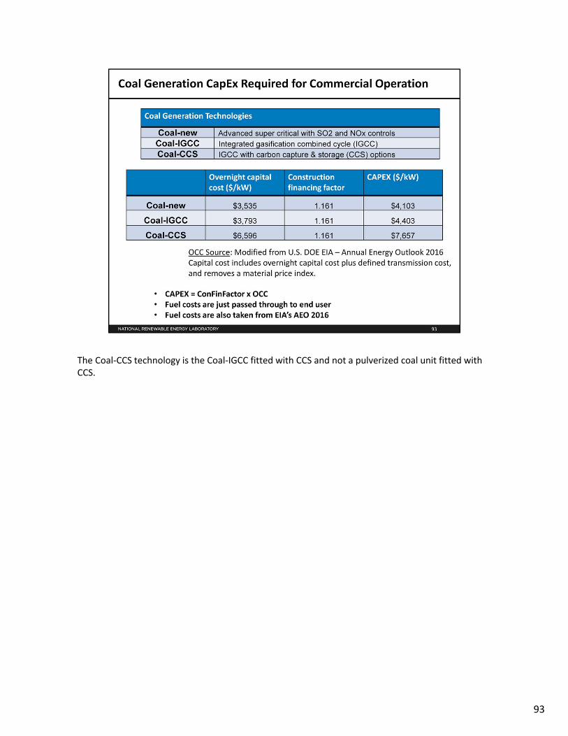
The Coal‐CCS technology is the Coal‐IGCC fitted with CCS and not a pulverized coal unit fitted with CCS.
93

94
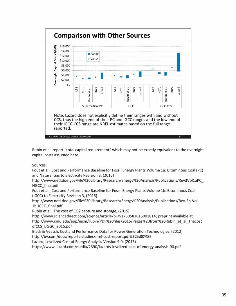
Rubin et al. report “total capital requirement” which may not be exactly equivalent to the overnight capital costs assumed here
Sources:Fout et al., Cost and Performance Baseline for Fossil Energy Plants Volume 1a: Bituminous Coal (PC) and Natural Gas to Electricity Revision 3, (2015) http://www.netl.doe.gov/File%20Library/Research/Energy%20Analysis/Publications/Rev3Vol1aPC_NGCC_final.pdfFout et al., Cost and Performance Baseline for Fossil Energy Plants Volume 1b: Bituminous Coal (IGCC) to Electricity Revision 3, (2015) http://www.netl.doe.gov/File%20Library/Research/Energy%20Analysis/Publications/Rev‐2b‐Vol‐1b‐IGCC_final.pdfRubin et al., The cost of CO2 capture and storage, (2015) http://www.sciencedirect.com/science/article/pii/S1750583615001814; preprint available at http://www.cmu.edu/epp/iecm/rubin/PDF%20files/2015/Pages%20from%20Rubin_et_al_ThecostofCCS_IJGGC_2015.pdfBlack & Veatch, Cost and Performance Data for Power Generation Technologies, (2012) http://bv.com/docs/reports‐studies/nrel‐cost‐report.pdf%E2%80%8ELazard, Levelized Cost of Energy Analysis‐Version 9.0, (2015) https://www.lazard.com/media/2390/lazards‐levelized‐cost‐of‐energy‐analysis‐90.pdf
95

96

97

The reference case does not include any carbon costs for conventional technologies. The LCOE of a CCS plant might be significantly reduced if it is able to sell the CO2 it has captured (e.g., and enhanced oil recovery operation may purchase CO2 from a CCS plant).
98

99

http://energy.gov/ne/nuclear‐reactor‐technologies/light‐water‐reactor‐sustainability‐lwrs‐programhttp://energy.gov/ne/about‐us/historyhttp://www.energy.gov/ne/nuclear‐reactor‐technologies
100

101
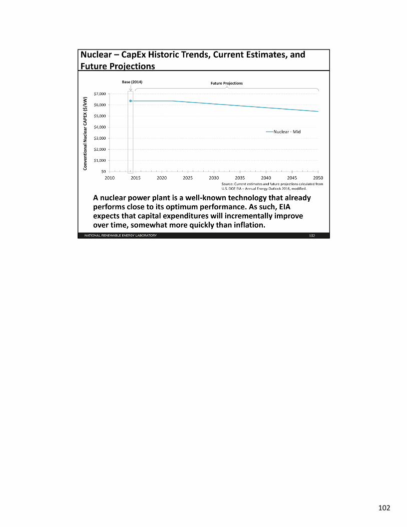
102

Sources:Black & Veatch, Cost and Performance Data for Power Generation Technologies, (2012) http://bv.com/docs/reports‐studies/nrel‐cost‐report.pdf%E2%80%8ELazard, Levelized Cost of Energy Analysis‐Version 9.0, (2015) https://www.lazard.com/media/2390/lazards‐levelized‐cost‐of‐energy‐analysis‐90.pdfEntergy, 2015 Integrated Resource Plan, (2015) http://entergy‐arkansas.com/content/transition_plan/IRP_Materials_Compiled.pdf
103

104

http://www.world‐nuclear.org/info/Nuclear‐Fuel‐Cycle/Introduction/Nuclear‐Fuel‐Cycle‐Overview/http://www.nei.org/Knowledge‐Center/Nuclear‐Statistics/US‐Nuclear‐Power‐Plants/US‐Nuclear‐Refueling‐Outage‐Dayshttp://www.nei.org/Knowledge‐Center/Nuclear‐Statistics/US‐Nuclear‐Power‐Plantshttp://www.nei.org/Knowledge‐Center/Nuclear‐Statistics/US‐Nuclear‐Power‐Plants/US‐Nuclear‐Capacity‐Factors
105
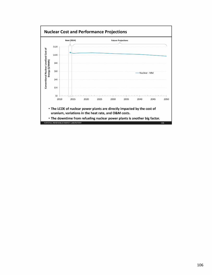
106

107

108

109

110

111

112

The reference case does not include any carbon costs for conventional technologies.
113

114
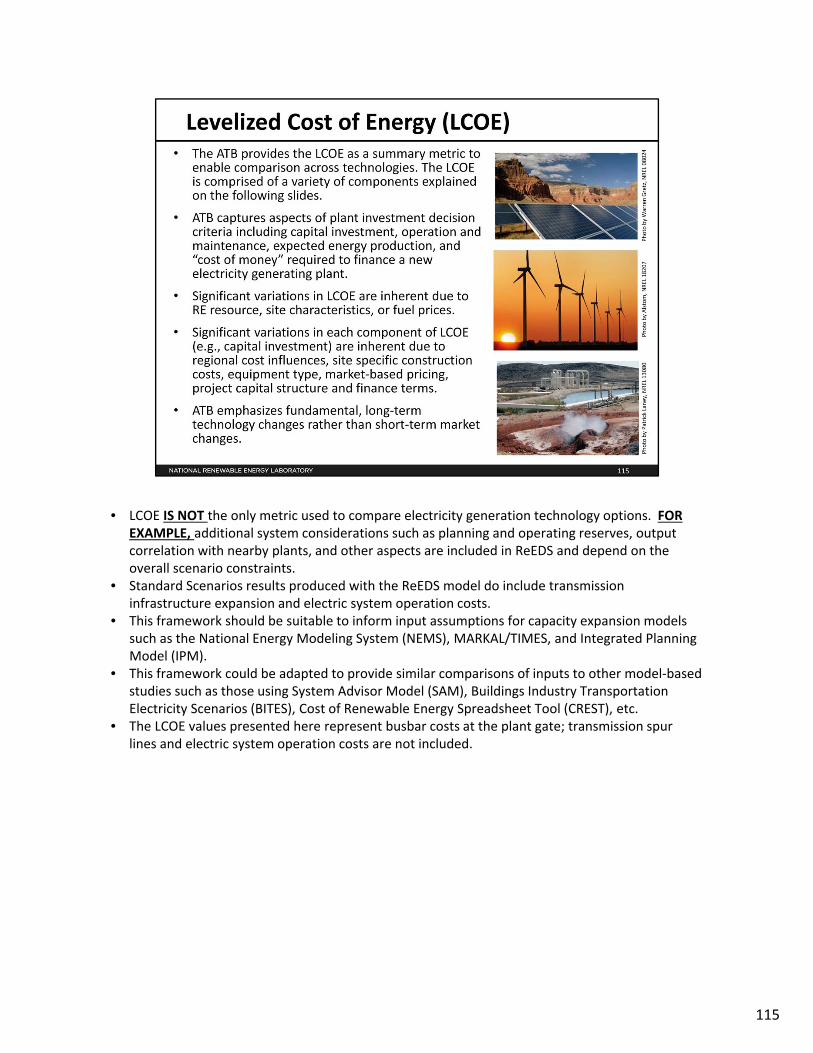
• LCOE IS NOT the only metric used to compare electricity generation technology options. FOREXAMPLE, additional system considerations such as planning and operating reserves, output correlation with nearby plants, and other aspects are included in ReEDS and depend on the overall scenario constraints.
• Standard Scenarios results produced with the ReEDS model do include transmission infrastructure expansion and electric system operation costs.
• This framework should be suitable to inform input assumptions for capacity expansion models such as the National Energy Modeling System (NEMS), MARKAL/TIMES, and Integrated Planning Model (IPM).
• This framework could be adapted to provide similar comparisons of inputs to other model‐based studies such as those using System Advisor Model (SAM), Buildings Industry Transportation Electricity Scenarios (BITES), Cost of Renewable Energy Spreadsheet Tool (CREST), etc.
• The LCOE values presented here represent busbar costs at the plant gate; transmission spur lines and electric system operation costs are not included.
115

• Variables are defined on Financial Definitions tab in ATB spreadsheet.• Levelized Cost of Energy (LCOE) selected to represent typical electricity generation cost
elements in common framework including project finance (FCR), capital expenditures (CAPEX), fixed and variable operation and maintenance costs (FOM and VOM), and annual energy production/kW plant capacity based on capacity factor (CF) and hours in a year (8760), and fuel costs.
• ATB spreadsheet and accompanying documentation illustrate range of LCOE for electricity generation technologies. Renewable generation technology cost range generally dictated by natural long‐term renewable resource characteristics. Fuel‐based technology cost range generally dictated by assumed range of future fuel cost.
• Project finance is represented using common assumptions for all technologies in order to focus differences on technical aspect. Depreciation is technology‐specific based on IRS tax code. Future ATB modifications to capture actual financing differences between technologies is under consideration.
• LCOE values in the ATB do not include any investment tax credit or production tax credit.
116

• For long‐term scenarios (through 2050) it is assumed that all electricity generation projects receive similar terms from lenders and equity investors. Although perceived level of risk across generation technologies may vary somewhat today, over the period of analysis, it is assumed that all technology options reach a common level of maturity and that there are no systematic differences in risk perception from the finance community. This assumption also focuses the scenario results on changes in the technology cost and performance.
• Future ATB modifications may include the ability to capture actual financing differences between technologies, in the short‐term.
• See Excel spreadsheet for equations, variable definitions, and parameters.
117
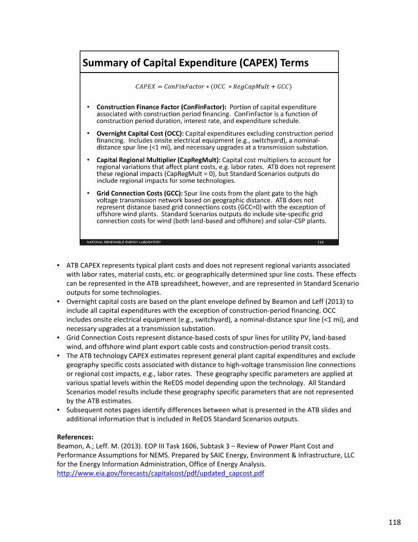
• ATB CAPEX represents typical plant costs and does not represent regional variants associated with labor rates, material costs, etc. or geographically determined spur line costs. These effects can be represented in the ATB spreadsheet, however, and are represented in Standard Scenario outputs for some technologies.
• Overnight capital costs are based on the plant envelope defined by Beamon and Leff (2013) to include all capital expenditures with the exception of construction‐period financing. OCC includes onsite electrical equipment (e.g., switchyard), a nominal‐distance spur line (<1 mi), and necessary upgrades at a transmission substation.
• Grid Connection Costs represent distance‐based costs of spur lines for utility PV, land‐based wind, and offshore wind plant export cable costs and construction‐period transit costs.
• The ATB technology CAPEX estimates represent general plant capital expenditures and exclude geography specific costs associated with distance to high‐voltage transmission line connections or regional cost impacts, e.g., labor rates. These geography specific parameters are applied at various spatial levels within the ReEDS model depending upon the technology. All Standard Scenarios model results include these geography specific parameters that are not represented by the ATB estimates.
• Subsequent notes pages identify differences between what is presented in the ATB slides and additional information that is included in ReEDS Standard Scenarios outputs.
References:Beamon, A.; Leff. M. (2013). EOP III Task 1606, Subtask 3 – Review of Power Plant Cost and Performance Assumptions for NEMS. Prepared by SAIC Energy, Environment & Infrastructure, LLC for the Energy Information Administration, Office of Energy Analysis. http://www.eia.gov/forecasts/capitalcost/pdf/updated_capcost.pdf
118

Some values are ranges because of capital costs that are site specific. For example, a low wind speed site may utilize a taller turbine with a higher capital cost compared to a high wind speed site.
119

Some values are ranges because of capital costs that are site specific. For example, a low wind speed site may utilize a taller turbine with a higher capital cost compared to a high wind speed site.
120

• Note that the range of capacity factors for conventional technologies represent the historical average across the entire U.S. fleet, by fuel type and generator type (lower value) and a value consistent with historic investment decision (upper value). Individual capacity factors for each plant’s actual operation will vary significantly.
• Capacity factors for RE technologies represent expected annual average annual energyproduction for a new plant installed in a given year over the lifetime of that plant. Inter‐annual variation in energy production is not represented.
• UPV capacity factors are for one‐axis tracking systems and are in terms of DC capacity to AC output.
121

• Note that the range of capacity factors for conventional technologies represent the historical average across the entire U.S. fleet, by fuel type and generator type (lower value) and a value consistent with historic investment decision (upper value). Individual capacity factors for each plant’s actual operation will vary significantly.
• Capacity factors for RE technologies represent expected annual average annual energyproduction for a new plant installed in a given year over the lifetime of that plant. Inter‐annual variation in energy production is not represented.
• UPV capacity factors are for one‐axis tracking systems and are in terms of DC capacity to AC output.
122

123
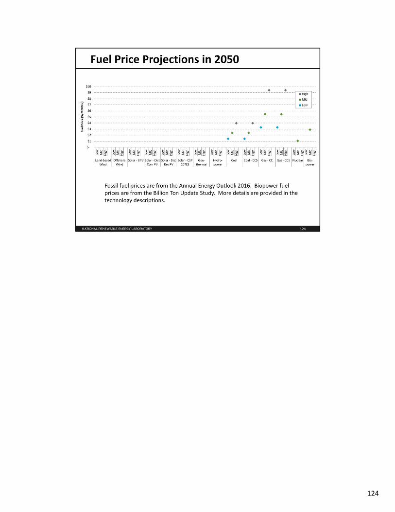
124

LCOE projections do not include any investment tax credit or production tax credit.
125

LCOE projections do not include any investment tax credit or production tax credit.
126
127

Values are for systems that come online in 2015. Values are overnight capital costs.
Hydropower is included in the non‐dispatchable portion because it is assumed that newhydropower plants will likely have less dispatchability than existing hydropower units.
Sources:Lazard: Levelized Cost of Energy Analysis 9.0 (https://www.lazard.com/media/2390/lazards‐levelized‐cost‐of‐energy‐analysis‐90.pdf)NREL: Annual Technology Baseline 2015 (http://www.nrel.gov/analysis/data_tech_baseline.html)EIA: Annual Energy Outlook 2015 (http://www.eia.gov/forecasts/aeo/pdf/0383(2015).pdf, see especially table 8.2 at https://www.eia.gov/forecasts/aeo/assumptions/pdf/table_8.2.pdf)
128
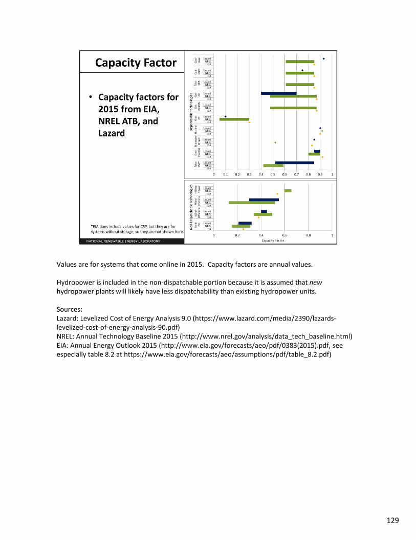
Values are for systems that come online in 2015. Capacity factors are annual values.
Hydropower is included in the non‐dispatchable portion because it is assumed that newhydropower plants will likely have less dispatchability than existing hydropower units.
Sources:Lazard: Levelized Cost of Energy Analysis 9.0 (https://www.lazard.com/media/2390/lazards‐levelized‐cost‐of‐energy‐analysis‐90.pdf)NREL: Annual Technology Baseline 2015 (http://www.nrel.gov/analysis/data_tech_baseline.html)EIA: Annual Energy Outlook 2015 (http://www.eia.gov/forecasts/aeo/pdf/0383(2015).pdf, see especially table 8.2 at https://www.eia.gov/forecasts/aeo/assumptions/pdf/table_8.2.pdf)
129
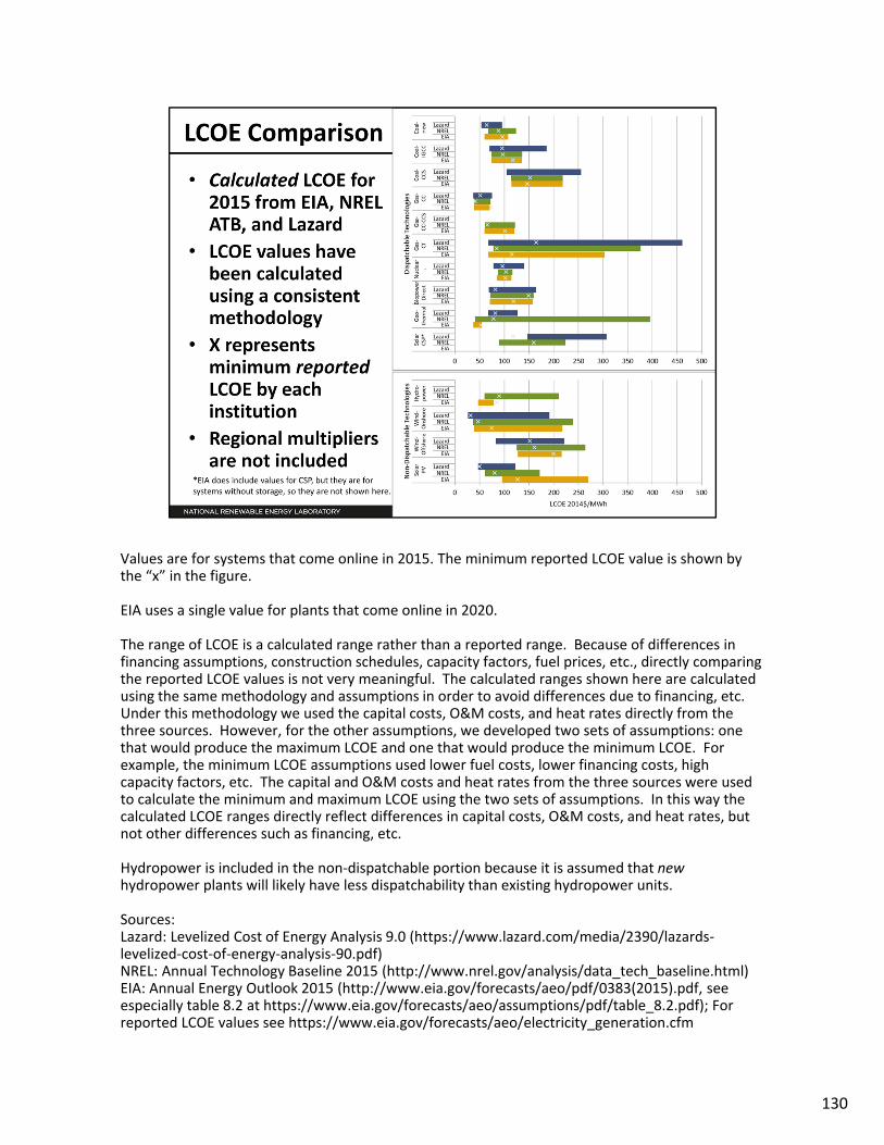
Values are for systems that come online in 2015. The minimum reported LCOE value is shown by the “x” in the figure.
EIA uses a single value for plants that come online in 2020.
The range of LCOE is a calculated range rather than a reported range. Because of differences in financing assumptions, construction schedules, capacity factors, fuel prices, etc., directly comparing the reported LCOE values is not very meaningful. The calculated ranges shown here are calculated using the same methodology and assumptions in order to avoid differences due to financing, etc. Under this methodology we used the capital costs, O&M costs, and heat rates directly from the three sources. However, for the other assumptions, we developed two sets of assumptions: one that would produce the maximum LCOE and one that would produce the minimum LCOE. For example, the minimum LCOE assumptions used lower fuel costs, lower financing costs, high capacity factors, etc. The capital and O&M costs and heat rates from the three sources were used to calculate the minimum and maximum LCOE using the two sets of assumptions. In this way the calculated LCOE ranges directly reflect differences in capital costs, O&M costs, and heat rates, but not other differences such as financing, etc.
Hydropower is included in the non‐dispatchable portion because it is assumed that newhydropower plants will likely have less dispatchability than existing hydropower units.
Sources:Lazard: Levelized Cost of Energy Analysis 9.0 (https://www.lazard.com/media/2390/lazards‐levelized‐cost‐of‐energy‐analysis‐90.pdf)NREL: Annual Technology Baseline 2015 (http://www.nrel.gov/analysis/data_tech_baseline.html)EIA: Annual Energy Outlook 2015 (http://www.eia.gov/forecasts/aeo/pdf/0383(2015).pdf, see especially table 8.2 at https://www.eia.gov/forecasts/aeo/assumptions/pdf/table_8.2.pdf); For reported LCOE values see https://www.eia.gov/forecasts/aeo/electricity_generation.cfm
130

131

132

133

134

Dollar year update is based on the consumer price index, which showed 1.6% inflation from 2013 to 2014.
135

136

137
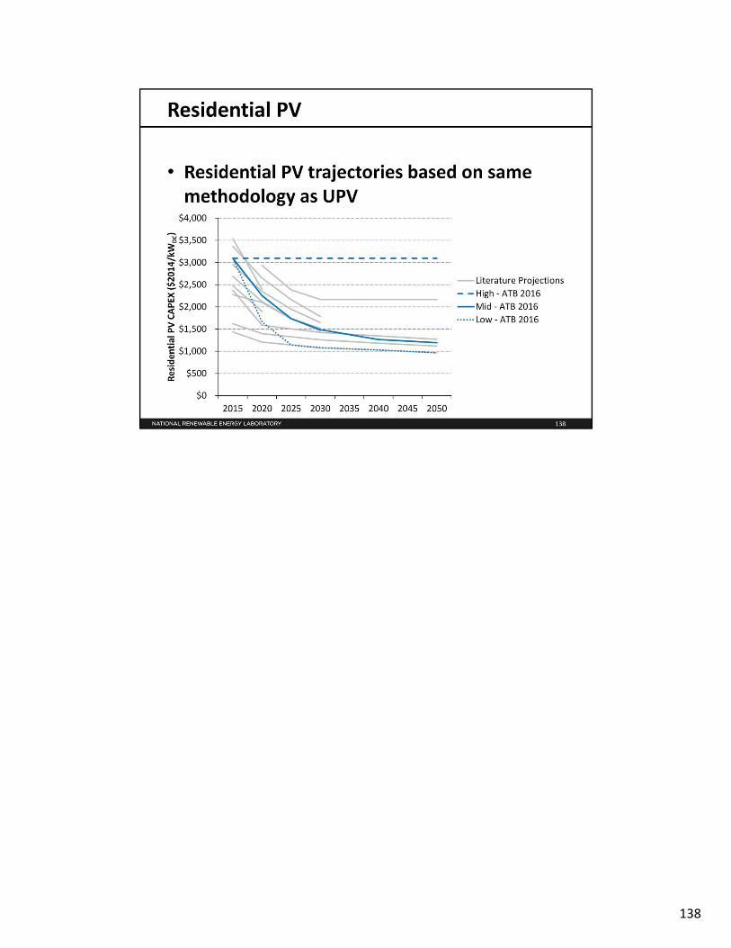
138
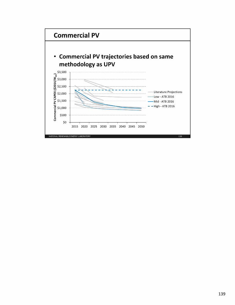
139

140

Last year’s ATB only included base year values.
Hydropower Vision report includes more detailed, bottom‐up, component cost bases for projections of future cost. Draft report currently in external review and publication planned for July 2016.
141

Last year’s ATB only included base year values and did not include projections. The learning rate results in a 10% cost reduction by 2035 for the low cost projection.
142
Conventional capital costs from the AEO 2016 Reference scenario declined linearly from 2030‐2040. This linear decline was simply extrapolated through 2050 to produce the 2040‐2050 cost projections.
143

144

145

146

147

148

149