Music Processing

Christof Wei and Meinard Mller

Lecture

Harmony Analysis

International Audio Laboratories Erlangen{christof.weiss,meinard.mueller}@audiolabs-erlangen.de

Book: Fundamentals of Music Processing

Meinard MllerFundamentals of Music ProcessingAudio, Analysis, Algorithms, Applications483 p., 249 illus., hardcoverISBN: 978-3-319-21944-8Springer, 2015

Accompanying website: www.music-processing.de

Book: Fundamentals of Music Processing

Meinard MllerFundamentals of Music ProcessingAudio, Analysis, Algorithms, Applications483 p., 249 illus., hardcoverISBN: 978-3-319-21944-8Springer, 2015

Accompanying website: www.music-processing.de

Book: Fundamentals of Music Processing

Meinard MllerFundamentals of Music ProcessingAudio, Analysis, Algorithms, Applications483 p., 249 illus., hardcoverISBN: 978-3-319-21944-8Springer, 2015

Accompanying website: www.music-processing.de

5.1 Basic Theory of Harmony5.2 Template-Based Chord Recognition5.3 HMM-Based Chord Recognition5.4 Further Notes

In Chapter 5, we consider the problem of analyzing harmonic properties of apiece of music by determining a descriptive progression of chords from a givenaudio recording. We take this opportunity to first discuss some basic theory ofharmony including concepts such as intervals, chords, and scales. Then,motivated by the automated chord recognition scenario, we introducetemplate-based matching procedures and hidden Markov modelsa conceptof central importance for the analysis of temporal patterns in time-dependentdata streams including speech, gestures, and music.

Chapter 5: Chord Recognition

Dissertation: Tonality-Based Style Analysis

Christof WeiComputational Methods for Tonality-Based Style Analysis of Classical Music Audio RecordingsPhD thesis, Ilmenau University of Technology, 2017

Chapter 5: Analysis Methods for Key and Scale StructuresChapter 6: Design of Tonal Features

Chromatic circle Shepards helix of pitch

Recall: Chroma Features Human perception of pitch is periodic Two components: tone height (octave) and chroma (pitch class)

Time (seconds)

Chr

oma

Recall: Chroma Features

Sal

ienc

e/

Like

lihoo

d

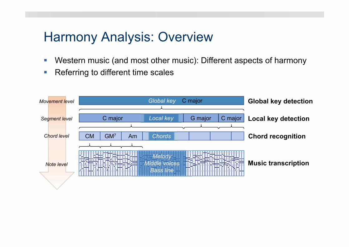
Harmony Analysis: Overview

ChordsCM GM7 Am

Global key

Local keyC major G major C major

Global key detection

Chord recognition

Music transcriptionNote level

Segment level

Chord level

Movement level C major

MelodyMiddle voices

Bass line

Local key detection

Western music (and most other music): Different aspects of harmony Referring to different time scales

Chord Recognition

Source: www.ultimate-guitar.com

Time (seconds)

Chord Recognition

Chord Recognition

Chord Recognition

C G

Audiorepresentation

Prefiltering

Compression Overtones Smoothing

Smoothing Transition HMM

Chromarepresentation

Patternmatching

Recognitionresult

Postfiltering

Majortriads

Minortriads

Chord Recognition: Basics Musical chord: Group of three or more notes

Combination of three or more tones which sound simultaneously

Types: triads (major, minor, diminished, augmented), seventh chords

Here: focus on major and minor triads

C

C Major (C)

Chord Recognition: Basics Musical chord: Group of three or more notes

Combination of three or more tones which sound simultaneously

Types: triads (major, minor, diminished, augmented), seventh chords

Here: focus on major and minor triads

Enharmonic equivalence: 12 different root notes possible 24 chords

C Major (C)

C Minor (Cm)

Chord Recognition: BasicsChords appear in different forms:

Inversions

Different voicings

Harmonic figuration: Broken chords (arpeggio)

Melodic figuration: Different melody note (suspension, passing tone, )

Further: Additional notes, incomplete chords

Chord Recognition: Basics

B

A

G

FE

D

C

G/A

D/E

C/D

A/B

F/G

C D D E E F G G A A B B

Templates: Major Triads

Chord Recognition: Basics

B

A

G

FE

D

C

G/A

D/E

C/D

A/B

F/G

C D D E E F G G A A B B

Templates: Major Triads

Chord Recognition: Basics

B

A

G

FE

D

C

G/A

D/E

C/D

A/B

F/G

Cm Cm Dm E m Em Fm Fm Gm Gm Am B m Bm

Templates: Minor Triads

Chroma vectorfor each audio frame

24 chord templates(12 major, 12 minor)

Compute for each frame thesimilarity of the chroma vector

to the 24 templates

B

A

G

F

E

D

C

G

D

C

A

F

C C D Cm Cm Dm

0 0 0 0 0 0

0 0 0 0 0 0

0 0 1 0 0 1

0 1 0 0 1 0

1 0 0 1 0 0

0 0 1 0 0 0

0 1 0 0 0 1

1 0 0 0 1 0

0 0 0 1 0 0

0 0 1 0 0 1

0 1 0 0 1 0

1 0 0 1 0 0

Chord Recognition: Template Matching

Chord Recognition: Template Matching Similarity measure: Cosine similarity (inner product of normalized

vectors)

Chord template:

Chroma vector:

Similarity measure:

Cho

rdC

hrom

a

Chord Recognition: Template Matching

Time (seconds)

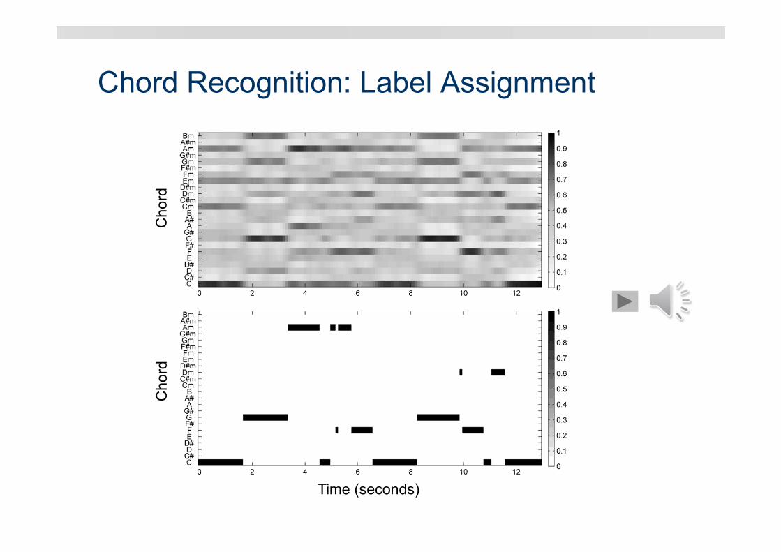
Chord Recognition: Label Assignment

Assign to each frame the chord labelof the template that maximizes the

similarity to the chroma vector

B

A

G

F

E

D

C

G

D

C

A

F

C C D Cm Cm Dm

0 0 0 0 0 0

0 0 0 0 0 0

0 0 1 0 0 1

0 1 0 0 1 0

1 0 0 1 0 0

0 0 1 0 0 0

0 1 0 0 0 1

1 0 0 0 1 0

0 0 0 1 0 0

0 0 1 0 0 1

0 1 0 0 1 0

1 0 0 1 0 0

Chroma vector

for each audio frame24 chord templates(12 major, 12 minor)

Compute for each frame thesimilarity of the chroma vector

to the 24 templates

Chord Recognition: Label Assignment

Cho

rdC

hord

Time (seconds)

Chord Recognition: Evaluation

Time (seconds)

C G Am F C G F C

Chord Recognition: Evaluation No-Chord annotations: not every frame labeled

Different evaluation measures:

Precision:

Recall:

F-Measure (balances precision and recall):

Without No-Chord label:

#TP#TP #FP

#TP#TP #FN

2

Chord Recognition: Smoothing Apply average filter of length :

Time (seconds)

Chord Recognition: Smoothing Apply average filter of length :

Time (seconds)

Chord Recognition: Smoothing Evaluation on all Beatles songs

0.8

0.75

0.7

0.65

0.6

0.55

0.5

0.45

0.4

0.35

Smoothing length

F-m

easu

re

Binary templates

1 5 9 13 17 21 25

Markov Chains Probabilistic model for sequential data

Markov property: Next state only depends on current state(no memory)

Consist of:

Set of states (hidden)

State transition probabilities

Initial state probabilitiesC

FG

0.8

0.60.7

0.2

0.1

0.3

0.10.1

0.1

Markov ChainsNotation:

C

FG

0.8

0.60.7

0.2

0.1

0.3

0.10.1

0.1

A 1 2 3123

State transition probabilities

Initial state probabilities

C 1 2 3

States for 1:

for 1:

Markov Chains Application examples:

Compute probability of a sequence using given a model (evaluation)

Compare two sequences using a given model

Evaluate a sequence with two different models (classification)

C

FG

0.8

0.60.7

0.2

0.1

0.3

0.10.1

0.1

Hidden Markov Models

C

FG

0.8

0.60.7

0.2

0.1

0.3

0.10.1

0.1

States as hidden variables

Consist of:

Set of states (hidden)

State transition probabilities

Initial state probabilities

Hidden Markov Models

C

FG

0.8

0.60.7

0.2

0.1

0.3

0.10.1

0.1

States as hidden variables

Consist of:

Set of states (hidden)

State transition probabilities

Initial state probabilities

Observations (visible)

Hidden Markov Models States as hidden variables

Consist of:

Set of states (hidden)

State transition probabilities

Initial state probabilities

Observations (visible)

Emission probabilities

0.7

0.1

0.9 0.2

0.3

0.8

C

FG

0.8

0.60.7

0.2

0.1

0.3

0.10.1

0.1

0

00

Hidden Markov ModelsNotation:

0.7

0.1

0.9 0.2

0.3

0.8

C

FG

0.8

0.60.7

0.2

0.1

0.3

0.10.1

0.1

0

00

A 1 2 3123

B 1 2 3123

State transition probabilities

Emission probabilities

Initial state probabilities

C 1 2 3

States for 1:

Observation symbols for 1:

Markov Chains Analogon: the students life

Consists of:

Set of states (hidden)

State transition probabilities

Initial state probabilities0.5

0.30.4

0.2

0.2

codingsleep

eatingsocialactivity

0.7

0.1

0.2

0.1 0.10.3 0

0.1

0.2

0.4

0.2

Hidden Markov Models Analogon: the students life

Consists of:

Set of states (hidden)

State transition probabilities

Initial state probabilities

Observations (visible)

Emission probabilities

0.5

0.30.4

0.2

0.2

codingsleep

eatingsocialactivity

0.7

0.1

0.2

0.1 0.10.3 0

0.1

0.2

0.4

0.2

0.9

Smell

NoiseLight

0.5

0.30.4

0.3

0.7

Hidden Markov Models Only observation sequence is visible!

Different algorithmic problems:

Evaluation problem Given: observation sequence and model

Calculate how well the model matches the sequence

Uncovering problem: Given: observation sequence and model

Find: optimal hidden state sequence

Estimation problem (training the HMM): Given: observation sequence

Find: model parameters

Baum-Welch algorithm (Expectation-Maximization)

Uncovering problem Given: observation sequence , , of length and

HMM (model parameters)

Find: optimal hidden state sequence , ,

Corresponds to chord estimation task!

Observation sequence

1 3 1 3 3 2

, , , , ,

Observation sequence

1 3 1 3 3 2

, , , , ,

1 1 1 3 3 1

Hidden state sequence , , , , ,

Uncovering problem Given: observation sequence , , of length and

HMM (model parameters)

Find: optimal hidden state sequence

Corresponds to chord estimation task!

Observation sequence

1 3 1 3 3 2

, , , , ,

C C C G G C

Hidden state sequence , , , , ,

Uncovering problem Given: observation sequence , , of length and

HMM (model parameters)

Find: optimal hidden state sequence

Corresponds to chord estimation task!

Uncovering problem Optimal hidden state sequence? Best explains given observation sequence

Maximizes probability ,

Straight-forward computation (naive approach):

Compute probability for each possible sequence

Number of possible sequences of length ( number of states):

Prob max ,

argmax ,

factorscomputationally infeasible!

Viterbi Algorithm Based on dynamic programming (similar to DTW)

Idea: Recursive computation from subproblems

Use truncated versions of observation sequence

Define , as the highest probability along a single state sequence, , that ends in state

Then, our solution is the state sequence yielding

Prob max :

,

1: , , , length 1:

, max, ,

1: , , , ,

Viterbi Algorithm : matrix of size

Recursive computation of , along the column index

Initialization:

1

Truncated observation sequence: 1 Current observation:

, 1 for some 1:

Viterbi Algorithm : matrix of size

Recursive computation of , along the column index

Recursion:

2:

Truncated observation sequence: 1: , , Last observation:

, 1: 1 , , , for 1:

, , 1

must be maximal!

Viterbi Algorithm : matrix of size

Recursive computation of , along the column index

Recursion:

2:

Truncated observation sequence: 1: , , Last observation:

, 1: 1 , , , for 1:

, , 1

must be maximal!

must be maximal (best index )

, max :

, 1

Viterbi Algorithm given find optimal state sequence , , , ,

Backtracking procedure (reverse order)

Last element:

Optimal state:

argmax :

,

Viterbi Algorithm given find optimal state sequence , , , ,

Backtracking procedure (reverse order)

Further elements:

1, 2, , 1 Optimal state:

argmax :

,

Viterbi Algorithm given find optimal state sequence , , , ,

Backtracking procedure (reverse order)

Further elements:

1, 2, , 1 Optimal state:

Simplification of backtracking: Keep track of maximizing index in

Define 1 matrix :

argmax :

,

, max :

, 1

, 1 argmax :

, 1

Viterbi AlgorithmSummary

1

1

2

3

4

5

6

7

8

, 1

1

States 1:

Sequenceindex 1:

Initialization

Viterbi AlgorithmSummary

1

1

2

3

4

5

6

7

8

n 1 n

, 1

1

States 1:

Sequenceindex 1:

Initialization Recursion

Viterbi AlgorithmSummary

1

1

2

3

4

5

6

7

8

n 1 n

,

, 1

1

States 1:

Sequenceindex 1:

Initialization Recursion

Viterbi AlgorithmSummary

1

1

2

3

4

5

6

7

8

n 1 n

, 1

,

, 1

1

States 1:

Sequenceindex 1:

Initialization Recursion

Viterbi AlgorithmSummary

1

2

3

4

5

6

7

8

n 1 n N

, 1

,

,

, 1

1

States 1:

Sequenceindex 1:

Initialization Recursion Termination

1

Viterbi AlgorithmSummary

1

1

2

3

4

5

6

7

8

n 1 n N

, 1

,

,

, 1

1

States 1:

Sequenceindex 1:

Initialization Recursion Termination

Backtrackingmatrix

Viterbi AlgorithmSummary

Viterbi Algorithm: Example

A 1 2 3123

B 1 2 3123

State transition probabilities Emission probabilities Initial state probabilities

C 1 2 3

Statesfor 1:

Observation symbolsfor 1:

HMM:

Viterbi Algorithm: Example

A 1 2 31 0.8 0.1 0.12 0.2 0.7 0.13 0.1 0.3 0.6

B 1 2 31 0.7 0 0.32 0.1 0.9 03 0 0.2 0.8

C 1 2 30.6 0.2 0.2

State transition probabilities Emission probabilities Initial state probabilities

Statesfor 1:

Observation symbolsfor 1:

HMM:

Viterbi Algorithm: Example

A 1 2 31 0.8 0.1 0.12 0.2 0.7 0.13 0.1 0.3 0.6

B 1 2 31 0.7 0 0.32 0.1 0.9 03 0 0.2 0.8

C 1 2 30.6 0.2 0.2

State transition probabilities Emission probabilities Initial state probabilities

Statesfor 1:

Observation symbolsfor 1:

HMM:

Observation sequence

1 3 1 3 3 2

O = (o1,o2,o3,o4,o5,o6)

Input

Viterbi Algorithm: Example

A 1 2 31 0.8 0.1 0.12 0.2 0.7 0.13 0.1 0.3 0.6

B 1 2 31 0.7 0 0.32 0.1 0.9 03 0 0.2 0.8

C 1 2 30.6 0.2 0.2

State transition probabilities Emission probabilities Initial state probabilities

Statesfor 1:

Observation symbolsfor 1:

HMM:

D o1= 1 o2= 3 o3= 1 o4= 3 o5= 3 o6= 2123

E o1= 1 o2= 3 o3= 1 o4= 3 o5= 3123

Observation sequence

1 3 1 3 3 2

O = (o1,o2,o3,o4,o5,o6)

Input Viterbi algorithm

Viterbi Algorithm: Example

A 1 2 31 0.8 0.1 0.12 0.2 0.7 0.13 0.1 0.3 0.6

B 1 2 31 0.7 0 0.32 0.1 0.9 03 0 0.2 0.8

C 1 2 30.6 0.2 0.2

State transition probabilities Emission probabilities Initial state probabilities

Statesfor 1:

Observation symbolsfor 1:

HMM:

D o1= 1 o2= 3 o3= 1 o4= 3 o5= 3 o6= 2123

E o1= 1 o2= 3 o3= 1 o4= 3 o5= 3123

Viterbi algorithm

, 1

Initialization

Viterbi Algorithm: Example

A 1 2 31 0.8 0.1 0.12 0.2 0.7 0.13 0.1 0.3 0.6

B 1 2 31 0.7 0 0.32 0.1 0.9 03 0 0.2 0.8

C 1 2 30.6 0.2 0.2

State transition probabilities Emission probabilities Initial state probabilities

Statesfor 1:

Observation symbolsfor 1:

HMM:

D o1= 1 o2= 3 o3= 1 o4= 3 o5= 3 o6= 21 0.42002 0.02003 0

E o1= 1 o2= 3 o3= 1 o4= 3 o5= 3123

Viterbi algorithm

, max :

, 1

, 1 argmax :

, 1

, 1

Initialization

Recursion

D o1= 1 o2= 3 o3= 1 o4= 3 o5= 3 o6= 21 0.4200 0.1008 0.0564 0.0135 0.0033 02 0.0200 0 0.0010 0 0 0.00063 0 0.0336 0 0.0045 0.0022 0.0003

E o1= 1 o2= 3 o3= 1 o4= 3 o5= 31 1 1 1 1 12 1 1 1 1 33 1 3 1 3 3

Viterbi algorithm

Viterbi Algorithm: Example

A 1 2 31 0.8 0.1 0.12 0.2 0.7 0.13 0.1 0.3 0.6

B 1 2 31 0.7 0 0.32 0.1 0.9 03 0 0.2 0.8

C 1 2 30.6 0.2 0.2

State transition probabilities Emission probabilities Initial state probabilities

Statesfor 1:

Observation symbolsfor 1:

HMM:

D o1= 1 o2= 3 o3= 1 o4= 3 o5= 3 o6= 2123

E o1= 1 o2= 3 o3= 1 o4= 3 o5= 3123

Viterbi algorithm

,

argmax :

,

Backtracking

D o1= 1 o2= 3 o3= 1 o4= 3 o5= 3 o6= 21 0.4200 0.1008 0.0564 0.0135 0.0033 02 0.0200 0 0.0010 0 0 0.00063 0 0.0336 0 0.0045 0.0022 0.0003

E o1= 1 o2= 3 o3= 1 o4= 3 o5= 31 1 1 1 1 12 1 1 1 1 33 1 3 1 3 3

i6 = 2

Viterbi algorithm

D o1= 1 o2= 3 o3= 1 o4= 3 o5= 3 o6= 21 0.4200 0.1008 0.0564 0.0135 0.0033 02 0.0200 0 0.0010 0 0 0.00063 0 0.0336 0 0.0045 0.0022 0.0003

E o1= 1 o2= 3 o3= 1 o4= 3 o5= 31 1 1 1 1 12 1 1 1 1 33 1 3 1 3 3

Viterbi algorithm

Viterbi Algorithm: Example

A 1 2 31 0.8 0.1 0.12 0.2 0.7 0.13 0.1 0.3 0.6

B 1 2 31 0.7 0 0.32 0.1 0.9 03 0 0.2 0.8

C 1 2 30.6 0.2 0.2

State transition probabilities Emission probabilities Initial state probabilities

Statesfor 1:

Observation symbolsfor 1:

HMM:

D o1= 1 o2= 3 o3= 1 o4= 3 o5= 3 o6= 2123

E o1= 1 o2= 3 o3= 1 o4= 3 o5= 3123

Viterbi algorithm

,

argmax :

,

Backtracking

Viterbi Algorithm: Example

A 1 2 31 0.8 0.1 0.12 0.2 0.7 0.13 0.1 0.3 0.6

B 1 2 31 0.7 0 0.32 0.1 0.9 03 0 0.2 0.8

C 1 2 30.6 0.2 0.2

State transition probabilities Emission probabilities Initial state probabilities

Statesfor 1:

Observation symbolsfor 1:

HMM:

Optimal state sequenceD o1= 1 o2= 3 o3= 1 o4= 3 o5= 3 o6= 21 0.4200 0.1008 0.0564 0.0135 0.0033 02 0.0200 0 0.0010 0 0 0.00063 0 0.0336 0 0.0045 0.0022 0.0003

E o1= 1 o2= 3 o3= 1 o4= 3 o5= 31 1 1 1 1 12 1 1 1 1 33 1 3 1 3 3

i6 = 2

Observation sequence

1 3 1 3 3 2

S* = (1,1,1,3,3,2)O = (o1,o2,o3,o4,o5,o6)

Input OutputViterbi algorithm

(a) Template Matching (frame-wise)

HMM: Application to Chord Recognition Effect of HMM-based chord estimation and smoothing:

C Dm G C

Time (seconds)Time (seconds)

(b) HMM

HMM: Application to Chord Recognition Parameters: Transition probabilities Estimated from data

State j

Sta

te

i

Log

prob

abilit

y

Parameters: Transition probabilities Estimated from data

Log

prob

abilit

y

Major chords Minor chords

Maj

or c

hord

sM

inor

cho

rds

HMM: Application to Chord Recognition

Major chords Minor chords

Maj

or c

hord

sM

inor

cho

rds

HMM: Application to Chord Recognition Parameters: Transition probabilities Transposition-invariant

Log

prob

abilit

y

HMM: Application to Chord Recognition Parameters: Transition probabilities Uniform transition matrix (only smoothing)

State j

Sta

te

i

Log

prob

abilit

y

HMM: Application to Chord Recognition Evaluation on all Beatles songs

0.8

0.75

0.7

0.65

0.6

0.55

0.5

0.45

0.4

0.35

Smoothing length

F-m

easu

re

binary

HMM

1 5 9 13 17 21 25

A

Cm

Em

Am

C

C

E G

E

B

E G

Em

C

B

CCmaj7

Chord Recognition: Further Challenges Chord ambiguities

Acoustic ambiguities (overtones)

Use advanced templates (model overtones, learned templates)

Enhanced chroma (logarithmic compression, overtone reduction)

Tuning inconsistency

Tonal Structures

ChordsCM GM7 Am

Global key

Local keyC major G major C major

Global key detection

Chord recognition

Music transcriptionNote level

Segment level

Chord level

Movement level C major

MelodyMiddle voices

Bass line

Local key detection

Local Key Detection

G

D

E

BD

E

F

A

GF

A

B

E mDm

BmFm

Cm

Gm

Dm

GmCm

Fm

Bm

EmAm

C

Key as an important musical concept (Symphony in C major)

Modulations Local approach

Key relations: Circle of fifth

Local Key Detection

Key as an important musical concept (Symphony in C major)

Modulations Local approach

Diatonic Scales

Simplification of keys

Perfect-fifth relation

1# diatonic

Circle of fifths

Local Key Detection Example: J.S. Bach, Choral "Durch Dein Gefngnis" (Johannespassion) Score Piano reduction

Local Key Detection Example: J.S. Bach, Choral "Durch Dein Gefngnis" (Johannespassion) Audio Waveform (Scholars Baroque Ensemble, Naxos 1994)

Time (seconds)

Local Key Detection: Chroma Features Example: J.S. Bach, Choral "Durch Dein Gefngnis" (Johannespassion) Audio Chroma features (Scholars Baroque Ensemble, Naxos 1994)

Local Key Detection: Chroma Smoothing Summarize pitch classes over a certain time

Chroma smoothing Parameters: blocksize b and hopsize h

bb

bh

h

Local Key Detection: Chroma Smoothing Choral (Bach)

Local Key Detection: Chroma Smoothing Choral (Bach) smoothed with b = 4.2 seconds and h = 1.5 seconds

Local Key Detection: Diatonic Scales Choral (Bach) Re-ordering to perfect fifth series

Local Key Detection: Diatonic Scales Choral (Bach) Re-ordering to perfect fifth series

Local Key Detection: Diatonic Scales Choral (Bach) Diatonic Scale Estimation (7 fifths)

4#

Local Key Detection: Diatonic Scales Choral (Bach) Diatonic Scale Estimation (7 fifths)

5#

Local Key Detection: Diatonic Scales Choral (Bach) Diatonic Scale Estimation: Multiply chroma values*

Local Key Detection: Diatonic Scales Choral (Bach) Diatonic Scale Estimation: Multiply chroma values

Local Key Detection: Diatonic Scales Choral (Bach) Diatonic Scale Estimation

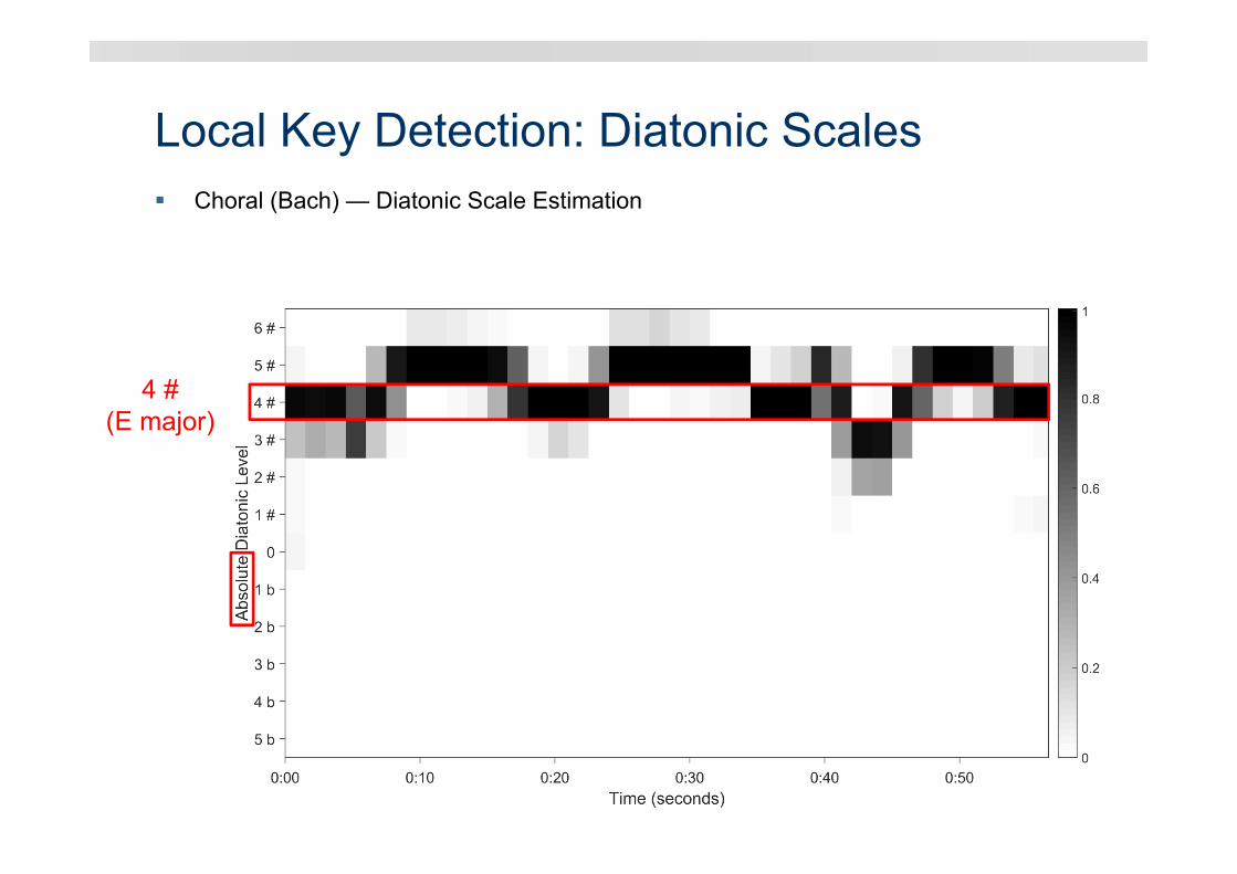
Local Key Detection: Diatonic Scales Choral (Bach) Diatonic Scale Estimation

4 #(E major)

Local Key Detection: Diatonic Scales Choral (Bach) Diatonic Scale Estimation: Shift to global key

4 #(E major)

Local Key Detection: Diatonic Scales Choral (Bach) 0 4#

Weiss / Habryka, Chroma-Based Scale Matchingfor Audio Tonality Analysis, CIM 2014

Local Key Detection: Examples L. v. Beethoven Sonata No. 10 op. 14 Nr. 2, 1. Allegro 0 1

(Barenboim, EMI 1998)

Local Key Detection: Examples R. Wagner, Die Meistersinger von Nrnberg, Vorspiel 0 0

(Polish National Radio Symphony Orchestra, J. Wildner, Naxos 1993)