202: dynamic macroeconomics -...

202: Dynamic MacroeconomicsNeoclassical Growth with Optimizing Agents (Ramsey-Cass-Koopmans

Model)

Mausumi Das

Delhi School of Economics

January 22-28-29 &Feb 2, 2015

Das (Delhi School of Economics) Dynamic Macro January 22-28-29 &Feb 2, 2015 1 / 39

Critique of Solow Model and Subsequent Extensions:

Recall the two basic critisisms of the Solow Model:

Even though it is supposed to be a growth model - it cannot reallyexplain long run growth:The steady state in the Solow model may be dynamically ineffi cient.

The basic Solow growth model has subsequently been extended tocounter some of these critisisms.

We have already looked at one such extension: Solow Model withExogenous Technological ProgressIn today’s class we shall look at the other extension: NeoclassicalGrowth Model with Optimizing Agents


Neoclassical Growth with Optimizing Agents:

Let us now extend the Solow model to allow for optimizing agents.

There are two frameworks which allow for optimizingconsumption/savings behaviour by households:

1 The Ramsey-Cass-Koopmans Inifinite Horizon Framework (henceforthR-C-K);

2 The Samuelson-Diamond Overlapping Generations Framework(henceforth OLG).

The basic difference between the two is that in the R-C-K modelagents optimize over infinite horizon; while in the OLG model, agentsoptimize over a finite time horizon (usually 2 periods).

As we shall see later, this apparently innocuous difference in terms oftime horizon spells out very different growth trajectories for the twomodels.


Neoclassical Growth with Optimizing Agents: The R-C-KModel

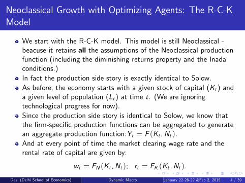
We start with the R-C-K model. This model is still Neoclassical -beacuse it retains all the assumptions of the Neoclassical productionfunction (including the diminishing returns property and the Inadaconditions.)In fact the production side story is exactly identical to Solow.As before, the economy starts with a given stock of capital (Kt) anda given level of population (Lt) at time t. (We are ignoringtechnological progress for now).Since the production side story is identical to Solow, we know thatthe firm-specific production functions can be aggregated to generatean aggregate production function:Yt = F (Kt ,Nt ).And at every point of time the market clearing wage rate and therental rate of capital are given by:

wt = FN (Kt ,Nt ); rt = FK (Kt ,Nt ).


The R-C-K Model: The Household Side Story

There are H identical households indexed by h.

Each household consists of a single infinitely lived member to beginwith (at t = 0). However population within a household increasesover time at a constant rate n. (And each newly born member isinfinitely lived too!) This implies that total population also increasesat the rate n.

At any point of time t, the total capital stock and the total labourforce in the economy are equally distributed across all the households,which are supplied inelastically to the market at the market wage ratewt and the market rental rate rt .

Thus total earning of a household at time t: wtNht + rtKht .

Corresponding per member earning: yht = wt + rtkht ,where kht is the per member capital stock in household h,

which is also the per capita capital stock (or the capital-labourratio, kt) in the economy.


The Household Side Story (Contd.):

In every time period, the instantaneous utility of the householddepends on its per member consumption:

ut = u(cht); u′ > 0; u′′ < 0; lim

ch→0u′(ch) = ∞; lim

ch→∞u′(ch) = 0.

The household at time 0 chooses its entire consumption profile{cht}∞t=0 so as to maximise the discounted sum of its life-time utility:

Uh0 =

∞∫t=0

u(cht)exp−ρt dt; ρ > 0,

subject to the household’s budget constraint in every time period.Notice that identical households implied that per memberconsumption (cht ) of any household is also equal to the per capitaconsumption (ct) in the economy at time t.


Interpretation of the Discount Rate:

Notice that the objective function of the household is an integraldefined over infinite horizon, where future utilities are discounted at aconstant rate ρ. The discount rate (ρ) may have three possibleinterpretations.

It is easier to understand these interpretations if we write down thediscrete time counterpart of the above objective function:

Uh0 ' u(ch0)+u(ch1)

1+ ρ+

u(ch2)

(1+ ρ)2+ .........

1. One interpretation of the above inifinte horizon utility function is thatagents are immortal (live for ever), but they have an innate(psychological) tendency to prefer current consumption over futureconsumption; hence they discount utilities from consumption thathappen in future dates. In this case ρ is interpreted as the "pure"rate of time preference of an agent.


Interpretation of the Discount Rate (Contd.):

Notice that the curvature of the utility function itself to some extentcaptures the preference of an agent over consumptions at two dates:t and t + 1. But this measure is ‘impure’in the sense that it dependson the precise amounts of the two consupmtions: cht and c

ht+1.

If I already have too much of cht and too little of cht+1, then I might

prefer an extra unit of future consumption more than an extra unit oftoday’s consumtion; and it would be the other way round if my cht istoo low compared to cht+1.This happens simply because the utility function is concave in c , whichinduces this kind on ‘consumption smoothing’.

A ‘pure’rate of time preference measures the agent’s preference forcurrent consumption over future consumption even when the actualconsumption at the two time periods are exactly equal (i.e., cht =cht+1). This way it neutralizes the effect of concavity of the utilityfunction and looks at the pure psychological preference for todayvis-a-vis tomorrow - which is independent of consumption smoothing.



In a two period set up where the total lifetime utility is defined byU(ct , ct+1), the ‘pure’rate time preference is defined as:

∂U∂ct− ∂U

∂ct+1∂U

∂ct+1

∣∣∣∣∣ct=ct+1=c

In other words, it measures the rate of change in the marginalvaluation on an extra unit of consumption available today vis-a-visavailable tomorrow - along a constant consumption path.It is easy to see that in our additive utility specification where

U(ct , ct+1) = u(ct ) +u(ct+1)1+ ρ

the above definition coincides with the discount rate ρ.



2. Another interpretation of the discount rate ρ follows if we read theinfinite horizon utility function of the household as the sum of utilitiesof successive generations of agents who themselves are finitely lived,but who care for their future generations.

To understand the idea better, suppose each member of thehousehold lives exactly for one period. But in every successive period(1+ n) proprtion of new members are born (also with a life-time ofexactly one period), each of whom are an exact replica of the previousset of agents (i.e, have identical tastes and preferences).

Each agent care for the utility of her child, who in turn care for theutility of her child and so on....In other words, the agents are altruistictowards their children. But the altruism is ‘imperfect’in the sensethat they care a little less for their children than they do forthemselves.

Das (Delhi School of Economics) Dynamic MacroJanuary 22-28-29 &Feb 2, 2015 10 /

39


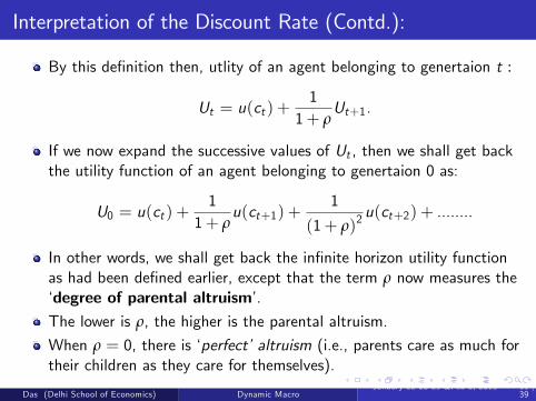
By this definition then, utlity of an agent belonging to genertaion t :

Ut = u(ct ) +1

1+ ρUt+1.

If we now expand the successive values of Ut , then we shall get backthe utility function of an agent belonging to genertaion 0 as:

U0 = u(ct ) +1

1+ ρu(ct+1) +

1

(1+ ρ)2u(ct+2) + ........

In other words, we shall get back the infinite horizon utility functionas had been defined earlier, except that the term ρ now measures the‘degree of parental altruism’.The lower is ρ, the higher is the parental altruism.

When ρ = 0, there is ‘perfect’altruism (i.e., parents care as much fortheir children as they care for themselves).


39


3. A third interpretation of the discount rate ρ follows if we allow eachagent to potentially live forever, but introduce an age-independentconstant mortality risk at every time period.

Suppose an agent lives for at the first period of his life (when he isborn); but at every subsequent period he faces a constant probablilityof dealth, denoted by p.If the agent is alive in any time period t, then he can enjoy utilityfrom consumption at that point of time, given by u(ct ). But if hedies then he gets zero utility.Thus beginning at time 0, the expected life-time utility of the agentwill be given by:

U0 = u(ct ) + pu(ct+1) + p2u(ct+2) + ........

Without any loss of generality, replace p by1

1+ ρand we shall get

back the infinite horizon utility function as had been defined earlier.Das (Delhi School of Economics) Dynamic Macro

January 22-28-29 &Feb 2, 2015 12 /39

The R-C-K Model: Centralized Version (Optimal Growth)

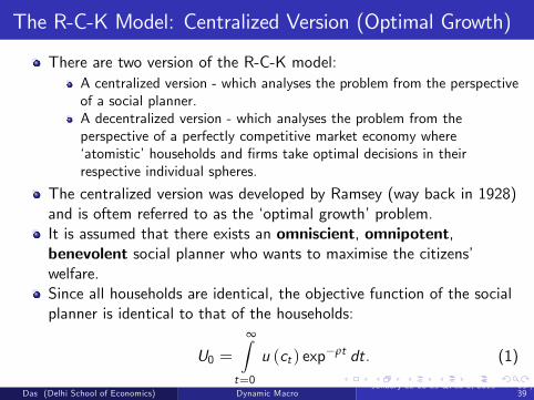
There are two version of the R-C-K model:A centralized version - which analyses the problem from the perspectiveof a social planner.A decentralized version - which analyses the problem from theperspective of a perfectly competitive market economy where‘atomistic’households and firms take optimal decisions in theirrespective individual spheres.

The centralized version was developed by Ramsey (way back in 1928)and is oftem referred to as the ‘optimal growth’problem.It is assumed that there exists an omniscient, omnipotent,benevolent social planner who wants to maximise the citizens’welfare.Since all households are identical, the objective function of the socialplanner is identical to that of the households:

U0 =

∞∫t=0

u (ct ) exp−ρt dt. (1)


39

The R-C-K Model: Centralized Version (Contd.)

The social planner maximises (1) subject to the planner’s budgetconstraint in every period.Notice that in a centrally planned economy there are no markets(hence no market wage rate or market rental rate), and there is noprivate ownership of assets (capital) and no personalized income.

The social planner employs the existing capital stock in the economy(either collectively owned or owned by the government) and theexisting labour force to produce the final output -using the aggregateproduction technology.

After production it distributes a part of the total output among itscitizens for consumption puoposes and invests the rest.

Thus the budget constraint faced by the planner in period t isnothing but the aggregate resource constraint:

Ct + It = Yt = F (Kt ,Nt ).


39


Investment augments next period’s capital stock:dKdt= It .

Thus the budget constraint faced by the planner in period t is givenby:

Ct +dKdt= F (Kt ,Nt )− δKt .

Writing in per capita terms:

ct +dkdt= f (kt )− δkt − nkt .

Thus the dynamic optimization problem of the social planner is:

∞∫t=0

u (ct ) exp−ρt dt (I)

subject to

dkdt= f (kt )− (δ+ n)kt − ct ; kt = 0 for all t; k0 given.


39

A Digression: Dynamic Optimization in Continuous Time(Optimal Control)

Consider the following optimization problem which is defined over afinite time horizon from 0 to T :

W =

T∫t=0

F (ut , xt , t) dt (2)

subject to

(i)dxdt= g(ut , xt , t); ut ∈ U; x0 given.

Here ut is called the control variable; xt is called the state variable; Frepresents the instantaneous payoff function, or the felicity function.

(i) specifies the evolution of the state variable as a function of thestate and control variables.

It is called the equation of motion or the state transition equation.


39

Optimal Control (Contd.):

The objective function here is an integral, and our task is to find outa time path of the time dependent variable u from the correspondingchoice set U, (i.e., to choose a u ∈ U for each point of time t startingfrom 0 to T ) such that the value of this integral is maximized.

But our choice is not unconstrained. (Had it been so, a simplepoint-by-point static optimization exercise would have given us therequired solution path).

Note that the F function depends not only on u but also on anothertime dependent variable x . And our choice of u at each point of timeaffects the next period’s value of x through the given differentialequation.

Thus our choice of u affects the objective function directly, as well asindirectly through x .


39


ut is called the control variable because we choosing its value directly.

Once the value of ut is chosen in any time period t, the value of thestate variable evolves automatically through the state transistionequation.

Notice that when we are considering the problem at time 0, the initialvalue of the state variable is given to us, but not that of the controlvariable.

The initial value of the control variable will also be optimallychosen, along with all its subsequent values.


39

Optimal Control: Pontryagin’s Maximum Principle

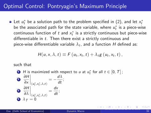
Let u∗t be a solution path to the problem specified in (2), and let x∗tbe the associated path for the state variable, where u∗t is a piece-wisecontinuous function of t and x∗t is a strictly continuous but piece-wisedifferentiable in t. Then there exist a strictly continuous andpiece-wise differentiable variable λt , and a function H defined as:

H(u, x ,λ, t) ≡ F (ut , xt , t) + λtg (ut , xt , t) ,

such that1 H is maximized with respect to u at u∗t for all t ∈ [0,T ] ;2

∂H∂x

∣∣∣∣(u∗t ,x

∗t ,λ,t)

= −dλ

dt;

3∂H∂λ

∣∣∣∣(u∗t ,x

∗t ,λ,t)

=dxdt;

4 λT = 0


39


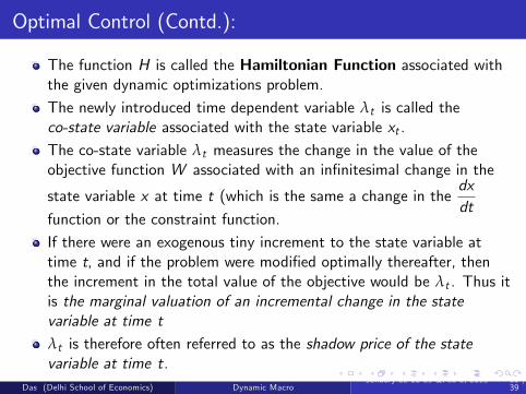
The function H is called the Hamiltonian Function associated withthe given dynamic optimizations problem.

The newly introduced time dependent variable λt is called theco-state variable associated with the state variable xt .

The co-state variable λt measures the change in the value of theobjective function W associated with an infinitesimal change in the

state variable x at time t (which is the same a change in thedxdt

function or the constraint function.

If there were an exogenous tiny increment to the state variable attime t, and if the problem were modified optimally thereafter, thenthe increment in the total value of the objective would be λt . Thus itis the marginal valuation of an incremental change in the statevariable at time t

λt is therefore often referred to as the shadow price of the statevariable at time t.


39


Pontryagin’s Maximum Principle gives us four first order necessaryconditions for the optimization problem defined in (2).These necessary conditions are also suffi cient if additionally thefollowing conditions (due to Mangasarian) hold:

the functions F and f are concave in (u, x);λt = 0 for all t whenever f is nonlinear in either u or x .

The first three F.O.N.C’s are defined in terms of the Hamiltonianfunction.Note that if the Hamiltonian function is non-linear in u, then (1) canbe replaced by the condition

∂H∂u

∣∣∣∣(u∗t ,x

∗t ,λ,t)

= 0,

provided the second order check is verified.The last condition of the Maximum Principle, which specifies aterminal condition for λt , is called the Transversality Condition.


39


Sometimes depending on the specification of the problem thetransversality condition may change.

In the above problem we are given an initial condition about the statestate variable, but nothing has be specified about the terminal valueof the state. This type of problems are called problems with a freeterminal state, and the relevant transversality condition for this setof problems are given by (4).

Alternatively you may have an optimization problem where not onlythe initial state value, but the terminal value of the state is alsogiven: xT = x (given).

This is a problem with a fixed terminal state. In this case the firstthree F.O.N.C.s will again be given by (1) — (3). Only condition (4)will be replaced by a new transversality condition now, given by

xT = x .


39


Yet another type of problem specifies a terminal condition on thestate variable in the form of an inequality. These are problems with atruncated vertical terminal line. : xT = x (given).In this case once again the first three F.O.N.C.s will again be given by(1) — (3). But condition (4) will be replaced by a new transversalitycondition now, given by the following Complementray Slacknesscondition:

λT = 0; xT = x ; λT (xT − x) = 0.


39

The R-C-K Model Revisited:

Let us now go back to the centralized version of the R-C-K model.Recall that the social planner’s problem is given by:

∞∫t=0

u (ct ) exp−ρt dt (I)

subject to

dkdt= f (kt )− (δ+ n)kt − ct ; kt = 0 for all t; k0 given.

Notice that the choice set for the control variable is: ct ∈ R+.Also the terminal condition on the state variable can be written as:limt→∞ kt = 0.Corresponding Hamiltonian Function:

Ht = u (ct ) exp−ρt +λt [f (kt )− (δ+ n)kt − ct ]


39


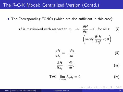
The Corresponding FONCs (which are also suffi cient in this case):

H is maximixed with respect to ct ⇒∂H∂ct

= 0 for all t; (i)(verify:

∂2H∂c2t

< 0)

∂H∂kt

= −dλ

dt; (ii)

∂H∂λt

=dkdt; (iii)

TVC: limt→∞

λtkt = 0. (iv)


39


Sometimes instead of the Hamiltonian Function, we use theCurrent-value Hamiltonian Function, defined as:

Ht = Ht expρt

= u (ct ) + µt [f (kt )− (δ+ n)kt − ct ] ,where µt = λt expρt is called the Current-value co-state variable.FONCs in terms of the Current-value Hamiltonian:

H is maximixed with respect to ct ⇒∂H∂ct

= 0 for all t; (i)

∂H∂kt

= −dµ

dt+ µρ; (ii)

∂H∂µt

=dkdt; (iii)

TVC: limt→∞

µt exp−ρt kt = 0. (iv)


39

Interpretation of the Optimality Conditions:

FONC (i):∂H∂ct

= 0⇒ u′ (ct ) = µt for all t

implies that the marginal utility from consumption at every point oftime must be equal to the shadow price of capital (i.e., theincremental utility associated with a unit increase in capital stock).

FONC (ii):

∂H∂kt

= −dµ

dt+ ρµt ⇒

[f ′(kt )− δ− n

]+1µt

dµ

dt= ρ

implies that the ‘net’rate of return (inclusive of capital gains/losses)on savings must be equal to the minimum compensation required toinduce people to forego a unit of current consumption for the sake oftomorrow (i.e., the agents’subjective rate of time preference).


39

Interpretation of the Optimality Conditions (Contd.):

FONC (iii):

∂H∂µt

=dkdt⇒ dk

dt= f (kt )− (δ+ n)kt − ct

denotes the per capita budget constraint of the social planner.Finally, the Transversality Condition:

limt→∞

µt exp−ρt kt = 0

implies that at the terminal timeif the shadow price of capital is positive, no capital stock should be leftunused (unconsumed) and the economy must end up with zero capitalstock (µT > 0⇒ kT = 0);on the other hand, if some capital stock is indeed left unused then itmust be the case that the corresponding shadow price is zero (i.e.,consuming further generates no utility value) (kT > 0⇒ µT = 0).Needless to say in this infinite horizon problem, the above conditionshold in a limiting sense.


39

Interpretation of the Current Value Hamiltonian Function:

The Current-value Hamiltonian Function:

Ht = u (ct ) + µt [f (kt )− (δ+ n)kt − ct ]measures the utility valuation of the per capita GDP at any point oftime t.Note that the per capita output at any time period f (kt ) can be usedfor two purposes: to be enjoyed as consumption (ct) and to augment

the capital stock(dkdt

).

The part that is consumed generates direct utility given by u (ct ) .That part that is used for investment generates potential futureconsumption and associated with an utility valuation of µt .Thus the Current Value Hamiltonian measures the direct as well asthe indirect utility associated with the per capita output at any timeperiod t.The Hamitonian (or the Present-value Hamiltonian), Ht , thenmeasures the present discounted value of the per capita output at anypoint of time t, measured in utility terms.Das (Delhi School of Economics) Dynamic Macro

January 22-28-29 &Feb 2, 2015 29 /39

R-C-K Model (Centralized Version): Characterization ofthe Optimal Path

To summarise, the optimal trajectories of ct , kt and µt must satisfythe following set of equations at every point of time t:

u′ (ct ) = µt ; (i)1µt

dµ

dt= ρ−

[f ′(kt )− δ− n

]; (ii)

dkdt

= f (kt )− (δ+ n)kt − ct ; (iii)

limt→∞

µt exp−ρt kt = 0. (iv)

Notice that even though we have three time-dependent variables (ct ,kt and µt ), ct and µt are always tied to each other by virtue ofequation (i); hence their dynamic paths are also inter-dependent.Thus we can eliminate one of them to get a system of differentialequations either in (ct and kt ) or in (kt and µt ).


39

Characterization of the Optimal Path (Contd.):

Here we shall eliminate µt and work with ct .(Verify that you reach the same conclusions when you eliminatect and work with µt instead).Log-differentiating (i), and using (ii):

u′′ (ct )u′ (ct )

dcdt

=1µt

dµ

dt= ρ−

[f ′(kt )− δ− n

]⇒ dc

dt=

ct(−ct u ′′(ct )u ′(ct )

) [f ′(kt )− δ− n− ρ]. (v)

We also know:dkdt= f (kt )− (δ+ n)kt − ct . (iii)

Equations (iii) & (v) represent a 2× 2 system of differential equationswhich along with the Transversality Condition characterize theoptimal path of the economy under the centralized R-C-K model.


39

Intertemporal Elasticity of Substitution:

Notice that in equation (v), there is a term:(−ct u′′ (ct )u′ (ct )

)≡ σ(ct ).

This term has multiple interpretations.

1 The most obvious interpretation is that it is the elasticity ofmarginal utility with respect to consumption.

2 In choices under uncertainty, σ(ct ) coincides with the Arrow-Prattmeasure of relative risk aversion.

3 The σ(ct ) terms is also the inverse of the elasticity ofsubstitution between current and future consumption.


39

Intertemporal Elasticity of Substitution (Contd.):

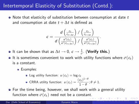
Note that elasticity of substitution between consumption at date tand consumption at date t + ∆t is defined as

ε =d(

ctct+∆t

)/(

ctct+∆t

)d(

u ′(ct )u ′(ct+∆t )

)/(

u ′(ct )u ′(ct+∆t )

) .It can be shown that as ∆t → 0, ε→ 1

σ . (Verify this.)It is sometimes convenient to work with utility functions where σ(ct )is a constant.

Examples:

Log utility function: u (ct ) = log ct

CRRA utility function: u (ct ) =(ct )1−θ

1− θ; θ 6= 1.

For the time being, however, we shall work with a general utilityfunction where σ(ct ) need not be a constant.


39

Characterization of the Optimal Path (Contd.):

The 2× 2 non-linear and autonomous system of equations for thecentralized economy are given by:

dcdt=

ctσ(ct )

[f ′(kt )− δ− n− ρ

]; (v)

anddkdt= f (kt )− (δ+ n)kt − ct . (iii)

Both (iii) and (v) are non-linear differential equations; so we have touse phase diagram technique to qualitatively characterize the optimalpath.


39

R-C-K Model (Centralized Version): Steady State(s)

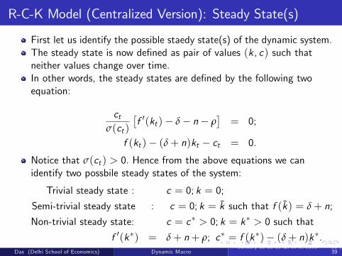
First let us identify the possible staedy state(s) of the dynamic system.The steady state is now defined as pair of values (k, c) such thatneither values change over time.In other words, the steady states are defined by the following twoequation:

ctσ(ct )

[f ′(kt )− δ− n− ρ

]= 0;

f (kt )− (δ+ n)kt − ct = 0.

Notice that σ(ct ) > 0. Hence from the above equations we canidentify two possbile steady states of the system:

Trivial steady state : c = 0; k = 0;

Semi-trivial steady state : c = 0; k = k such that f (k) = δ+ n;

Non-trivial steady state: c = c∗ > 0; k = k∗ > 0 such that

f ′(k∗) = δ+ n+ ρ; c∗ = f (k∗)− (δ+ n)k∗.Das (Delhi School of Economics) Dynamic Macro

January 22-28-29 &Feb 2, 2015 35 /39

R-C-K Model (Centralized Version): Constrcution of thePhase Diagram

From equation (v):

dcdt

T 0 according as

either ct = 0 or f ′(kt ) T δ+ n+ ρ.

On the other hand, from equation (iii):

dkdt

T 0 according as

ct S f (kt )− (δ+ n)kt .

Now we can trace the level curvesdcdt= 0 and

dkdt= 0 in the (kt , ct )

plane and draw the coresponding directional arrows to get thecorresponding phase diagram.(How should the Phase Diagram look?)


39

R-C-K Model (Centralized Version): Phase Diagram


39

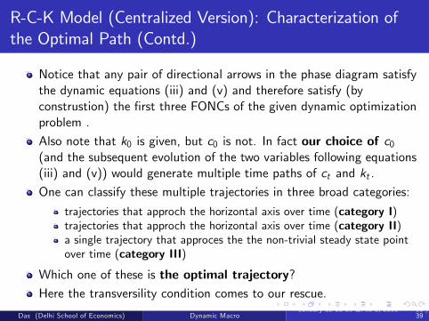
R-C-K Model (Centralized Version): Characterization ofthe Optimal Path (Contd.)

Notice that any pair of directional arrows in the phase diagram satisfythe dynamic equations (iii) and (v) and therefore satisfy (byconstrustion) the first three FONCs of the given dynamic optimizationproblem .

Also note that k0 is given, but c0 is not. In fact our choice of c0(and the subsequent evolution of the two variables following equations(iii) and (v)) would generate multiple time paths of ct and kt .

One can classify these multiple trajectories in three broad categories:

trajectories that approch the horizontal axis over time (category I)trajectories that approch the horizontal axis over time (category II)a single trajectory that approces the the non-trivial steady state pointover time (category III)

Which one of these is the optimal trajectory?Here the transversility condition comes to our rescue.


39

R-C-K Model (Centralized Version): Characterization ofthe Optimal Path (Contd.)

Recall that the TVC is part of the necessary (and suffi cinet)conditions for optimality.

So among all these trajectories, the one which satisfies the TVC willindeed be the optimal path. (What is there are multiple suchtrajectories?)

As it turns out, only the trajectory belonging to category III satisfiesall the four FONCs including the transversility condition. (Proof?)Thus, given k0, it is optimal for the social planner to choose thecorresponding c0 that lies on trajectory III and then let the economyevolve following the two dynamic equations (iii) & (v).

Growth Implications?Dynamic Effi ciency of the Steady State?


39

202: dynamic macroeconomics -...

Documents