2020 annual markets report
TRANSCRIPT

ISO-NE PUBLIC
2020 Annual Markets Report © ISO New England Inc. Internal Market Monitor
JUNE 9, 2021

Document Revision History
Date Version Remarks
06/09/2021 Original Initial Posting

2020 Annual Markets Report page iii ISO-NE PUBLIC
Preface/Disclaimer
The Internal Market Monitor (IMM) of ISO New England (ISO) publishes an Annual Markets Report (AMR) that assesses the state of competition in the wholesale electricity markets operated by the ISO. The 2020 Annual Markets Report covers the ISO’s most recent operating year, January 1 to December 31, 2020. The report addresses the development, operation, and performance of the wholesale electricity markets administered by the ISO and presents an assessment of each market based on market data, performance criteria, and independent studies.
This report fulfills the requirement of Market Rule 1, Appendix A, Section III.A.17.2.4, Market Monitoring, Reporting, and Market Power Mitigation:
The Internal Market Monitor will prepare an annual state of the market report on market trends and the
performance of the New England Markets and will present an annual review of the operations of the New
England Markets. The annual report and review will include an evaluation of the procedures for the
determination of energy, reserve and regulation clearing prices, Net Commitment-Period Compensation
costs and the performance of the Forward Capacity Market and Financial Transmission Rights Auctions. The
review will include a public forum to discuss the performance of the New England Markets, the state of
competition, and the ISO’s priorities for the coming year. In addition, the Internal Market Monitor will
arrange a non-public meeting open to appropriate state or federal government agencies, including the
Commission and state regulatory bodies, attorneys general, and others with jurisdiction over the competitive
operation of electric power markets, subject to the confidentiality protections of the ISO New England
Information Policy, to the greatest extent permitted by law.1
This report is being submitted simultaneously to the ISO and the Federal Energy Regulatory Commission (FERC) per FERC order:
The Commission has the statutory responsibility to ensure that public utilities selling in competitive bulk
power markets do not engage in market power abuse and also to ensure that markets within the
Commission’s jurisdiction are free of design flaws and market power abuse. To that end, the Commission will
expect to receive the reports and analyses of a Regional Transmission Organization’s market monitor at the
same time they are submitted to the RTO.2
This report presents the most important findings, market outcomes, and market design changes of New England’s wholesale electricity markets for 2020. Section 1 summarizes the region’s wholesale electricity market outcomes, the important market issues and our recommendations for addressing these issues. It also addresses the overall competitiveness of the markets, and market mitigation and market reform activities. Sections 2 through Section 8 include more detailed discussions of each of the markets, market results, analysis and recommendations. A list of acronyms and abbreviations is included at the back of the report.
1 ISO New England Inc. Transmission, Markets, and Services Tariff (ISO tariff), Section III.A.17.2.4, Market Rule 1, Appendix A, “Market Monitoring, Reporting, and Market Power Mitigation”, http://www.iso-ne.com/static-assets/documents/regulatory/tariff/sect_3/mr1_append_a.pdf.
2 FERC, PJM Interconnection, L.L.C. et al., Order Provisionally Granting RTO Status, Docket No. RT01-2-000, 96 FERC ¶ 61, 061 (July 12, 2001).

2020 Annual Markets Report page iv ISO-NE PUBLIC
A number of external and internal audits are also conducted each year to ensure that the ISO followed the approved market rules and procedures and to provide transparency to New England stakeholders. Further details of these audits can be found on the ISO website.3
All information and data presented are the most recent as of the time of writing. The data presented in this report are not intended to be of settlement quality and some of the underlying data used are subject to resettlement.
In case of a discrepancy between this report and the ISO New England Tariff or Procedures, the meaning of the Tariff and Procedures shall govern.
Underlying natural gas data are furnished by the Intercontinental Exchange (ICE):
Underlying oil and coal pricing data are furnished by Argus Media.
3 See https://www.iso-ne.com/about/corporate-governance/financial-performance

2020 Annual Markets Report page v ISO-NE PUBLIC
Contents
Preface/Disclaimer ............................................................................................................................................... iii
Contents ................................................................................................................................................................ v
Figures .................................................................................................................................................................. ix
Tables .................................................................................................................................................................. xii
Section 1 Executive Summary .............................................................................................................................. 13
1.1 Wholesale Cost of Electricity ............................................................................................................................. 18
1.2 Overview of Supply and Demand Conditions .................................................................................................... 20
1.3 Day-Ahead and Real-Time Energy Markets ....................................................................................................... 29
1.4 Forward Capacity Market (FCM) ....................................................................................................................... 34
1.5 Ancillary Services Markets ................................................................................................................................. 37
1.6 IMM Market Enhancement Recommendations ................................................................................................ 38
Section 2 Overall Market Conditions .................................................................................................................... 42
2.1 Wholesale Cost of Electricity ............................................................................................................................. 42
2.2 Supply Conditions .............................................................................................................................................. 44
2.2.1 Generation and Capacity Mix .................................................................................................................... 44
2.2.2 Generation Fuel and Emissions Costs ........................................................................................................ 50
2.2.3 Generator Profitability ............................................................................................................................... 58
2.2.4 Energy Demand .......................................................................................................................................... 60
2.2.5 Reserve Requirements ............................................................................................................................... 64
2.2.6 Capacity Market Requirements ................................................................................................................. 65
2.3 Imports and Exports (External Transactions) .................................................................................................... 67
Section 3 Day-Ahead and Real-Time Energy Market ............................................................................................ 71
3.1 Overview of the Day-Ahead and Real-Time Energy Markets ............................................................................ 72
3.2 Energy and NCPC (Uplift) Payments .................................................................................................................. 74
3.3 Energy Prices ..................................................................................................................................................... 74
3.3.1 Hub Prices .................................................................................................................................................. 75
3.3.2 Zonal Prices ................................................................................................................................................ 76
3.3.3 Load-Weighted Prices ................................................................................................................................ 77
3.3.4 Fast Start Pricing: Impact on Real-Time Energy Prices .............................................................................. 79
3.3.5 Energy Price Convergence between the Day-Ahead and Real-Time Market ............................................. 80
3.4 Drivers of Energy Market Outcomes ................................................................................................................. 85
3.4.1 Generation Costs ....................................................................................................................................... 85
3.4.2 Supply-Side Participation ........................................................................................................................... 92
3.4.3 Reserve Adequacy Analysis Commitments ................................................................................................ 94

2020 Annual Markets Report page vi ISO-NE PUBLIC
3.4.4 Load and Weather Conditions ................................................................................................................... 95
3.4.5 Demand Bidding......................................................................................................................................... 99
3.4.6 Load Forecast Error .................................................................................................................................. 101
3.4.7 Reserve Margin ........................................................................................................................................ 105
3.4.8 System Events during 2020 ...................................................................................................................... 106
3.4.9 Reliability Commitments and Posturing .................................................................................................. 112
3.4.10 Congestion ............................................................................................................................................. 116
3.4.11 Marginal Resources ............................................................................................................................... 124
3.5 Net Commitment Period Compensation ......................................................................................................... 128
3.5.1 Uplift Payment Categories ....................................................................................................................... 128
3.5.2 Uplift Payments for 2016 to 2020 ............................................................................................................ 129
3.6 Demand Resource Participation in the Energy and Capacity Markets ............................................................ 133
3.6.1 Energy Market Offers and Dispatch under PRD ....................................................................................... 134
3.6.2 NCPC and Energy Market Compensation under PRD .............................................................................. 136
3.6.3 Capacity Market Participation under PRD ............................................................................................... 137
3.7 Market Structure and Competitiveness .......................................................................................................... 138
3.7.1 C4 Concentration Ratio for Generation ................................................................................................... 139
3.7.2 C4 Concentration Ratio for Load.............................................................................................................. 140
3.7.3 Residual Supply Index and the Pivotal Supplier Test ............................................................................... 141
3.7.4 Day-Ahead Price-Cost Markup ................................................................................................................. 143
3.8 Energy Market Mitigation ............................................................................................................................... 144
3.8.1 Types of Mitigation .................................................................................................................................. 144
3.8.2 Mitigation Event Hours ............................................................................................................................ 146
Section 4 Virtual Transactions and Financial Transmission Rights ...................................................................... 150
4.1 Virtual Transactions ......................................................................................................................................... 150
4.1.1 Virtual Transaction Overview .................................................................................................................. 151
4.1.2 Virtual Transactions and NCPC ................................................................................................................ 152
4.1.3 Virtual Transaction Profitability ............................................................................................................... 152
4.1.4 Price Convergence and Virtual Transaction Volumes .............................................................................. 155
4.1.5 The Impact of Market Rule Changes ........................................................................................................ 157
4.2 Financial Transmission Rights .......................................................................................................................... 158
4.2.1 FTR Overview ........................................................................................................................................... 159
4.2.2 FTR Market Volume ................................................................................................................................. 162
4.2.3 FTR Funding ............................................................................................................................................. 164
4.2.4 FTR Market Concentration ....................................................................................................................... 165

2020 Annual Markets Report page vii ISO-NE PUBLIC
4.2.5 FTR Profitability........................................................................................................................................ 165
Section 5 External Transactions ......................................................................................................................... 169
5.1 External Transactions with New York and Canada .......................................................................................... 170
5.2 Bidding and Scheduling ................................................................................................................................... 172
5.3 External Transaction Uplift (Net Commitment Period Compensation) Credits............................................... 176
5.4 Coordinated Transaction Scheduling ............................................................................................................... 177
Section 6 Forward Capacity Market ................................................................................................................... 184
6.1 Forward Capacity Market Overview ................................................................................................................ 186
6.2 Capacity Market Payments .............................................................................................................................. 189
6.2.1 Payments by Commitment Period ........................................................................................................... 189
6.2.2 Pay-for-Performance Outcomes .............................................................................................................. 190
6.2.3 Delayed Commercial Operation Rules ..................................................................................................... 190
6.3 Review of the Fifteenth Forward Capacity Auction (FCA 15) .......................................................................... 191
6.3.1 Qualified and Cleared Capacity ................................................................................................................ 191
6.3.2 Results and Competitiveness ................................................................................................................... 193
6.3.3 Results of the Substitution Auction (CASPR) ........................................................................................... 195
6.4 Forward Capacity Market Outcomes............................................................................................................... 195
6.4.1 Forward Capacity Auction Outcomes ...................................................................................................... 196
6.4.2 Secondary Forward Capacity Market Results .......................................................................................... 199
6.5 Trends in Capacity Supply Obligations ............................................................................................................ 200
6.5.1 Retirement of Capacity Resources ........................................................................................................... 201
6.5.2 New Entry of Capacity Resources ............................................................................................................ 202
6.6 Market Competitiveness ................................................................................................................................. 204
6.7 Capacity Market Mitigation ............................................................................................................................. 209
6.7.1 Supplier-Side Market Power .................................................................................................................... 209
6.7.2 Test Price Review ..................................................................................................................................... 211
6.7.3 Minimum Offer Price Rule ....................................................................................................................... 212
Section 7 Ancillary Services ................................................................................................................................ 214
7.1 Real-Time Operating Reserves ........................................................................................................................ 215
7.1.1 Real-Time Operating Reserve and Pricing Mechanics ............................................................................. 215
7.1.2 Real-Time Operating Reserve Payments ................................................................................................. 217
7.1.3 Real-Time Operating Reserve Prices: Frequency and Magnitude ........................................................... 219
7.2 Forward Reserves ............................................................................................................................................ 221
7.2.1 Market Requirements .............................................................................................................................. 222
7.2.2 Auction Results ........................................................................................................................................ 225

2020 Annual Markets Report page viii ISO-NE PUBLIC
7.2.3 FRM Payments ......................................................................................................................................... 226
7.2.4 Structural Competitiveness ..................................................................................................................... 227
7.3 Regulation ....................................................................................................................................................... 229
7.3.1 Regulation Prices ..................................................................................................................................... 230
7.3.2 Regulation Payments ............................................................................................................................... 231
7.3.3 Requirements and Performance .............................................................................................................. 232
7.3.4 Regulation Market Structural Competitiveness ....................................................................................... 232
Section 8 Market Design or Rule Changes .......................................................................................................... 235
8.1 Major Design Changes Recently Implemented ............................................................................................... 235
8.1.1 Nested Export Capacity Zones ................................................................................................................. 235
8.1.2 Energy Market Offer Caps ........................................................................................................................ 236
8.1.3 First Competitive Solicitation for Transmission Needs under FERC Order 1000 ..................................... 237
8.1.4 Removal of Energy Efficiency Resources from Pay-for-Performance Obligations and Settlement ......... 237
8.2 Major Design or Rule Changes in Development or Implementation for Future Years .................................... 238
8.2.1 Interim Compensation Treatment ........................................................................................................... 238
8.2.2 FCA Parameters Review ........................................................................................................................... 239
8.2.3 Removal of Appendix B from Tariff .......................................................................................................... 240
8.2.4 Removal of Price-Lock from the Forward Capacity Market ..................................................................... 241
8.2.5 Transmission Cost Allocation to Network Customers with Behind-the-Meter Generation .................... 241
8.2.6 Order 2222, Distributed Energy Resources.............................................................................................. 242
8.2.7 New England's Future Grid Initiative ....................................................................................................... 243
Acronyms and Abbreviations ............................................................................................................................. 244
2020 Annual Markets Report page ix ISO-NE PUBLIC
Figures
Figure 1-1: Historical Electricity Prices, Wholesale Load and Natural Gas Prices ........................................................ 14 Figure 1-2: Wholesale Costs and Average Natural Gas Prices ..................................................................................... 18 Figure 1-3: Annual and Quarterly Generation Costs, Day-Ahead LMP and Spark Spreads (On-Peak Periods) ........... 22 Figure 1-4: Estimated Revenue and Profitability for New Gas-fired Generators ........................................................ 23 Figure 1-5: Annual Estimated Average Costs of Generation and CO2 Emissions ......................................................... 25 Figure 1-6: Average Quarterly Weather-Normalized Load with Energy Efficiency and Solar Impacts ....................... 26 Figure 1-7: Average Generator Capacity by Fuel Type ................................................................................................ 28 Figure 1-8: Cleared and Surplus Capacity in FCA 8 through FCA 15 ............................................................................ 29 Figure 1-9: Day-Ahead Energy Market Load-Weighted Prices .................................................................................... 30 Figure 1-10: Total Uplift Payments by Year and Category ........................................................................................... 31 Figure 1-11: FCM Payments and Capacity Surplus by Commitment Period ................................................................ 35 Figure 2-1: Wholesale Costs ($ billions and $/MWh) and Average Natural Gas Prices ............................................... 43 Figure 2-2: Average Output and Share of Native Electricity Generation by Fuel Type................................................ 45 Figure 2-3: Capacity Factor by Fuel Type ..................................................................................................................... 46 Figure 2-4: Average Native Electricity Generation and Load by State, 2016 and 2020 ............................................... 47 Figure 2-5: Average Generator Capacity by Fuel Type ................................................................................................ 48 Figure 2-6: Average Age of New England Generator Capacity by Fuel Type (2016-2020) .......................................... 49 Figure 2-7: Generation Additions, Retirements and FCM Outcomes .......................................................................... 50 Figure 2-8: Average Fuel Prices by Quarter and Year .................................................................................................. 51 Figure 2-9: New England vs. Henry Hub and Marcellus Natural Gas Prices ................................................................ 52 Figure 2-10: Annual Estimated Average Costs of Generation and Emissions .............................................................. 53 Figure 2-11: Estimated Average Cost of RGGI CO2 Allowances and Contribution of Energy Production Costs .......... 54 Figure 2-12: Contributions of Emissions Cost to Energy Production Costs ................................................................. 56 Figure 2-13: GWSA Allowance Trading Activity, 2018-2020 ........................................................................................ 57 Figure 2-14: Estimated Net Revenue for New Gas-fired Generators .......................................................................... 59 Figure 2-15: Average Hourly Load by Quarter and Year .............................................................................................. 61 Figure 2-16: Load Duration Curves .............................................................................................................................. 62 Figure 2-17: Average Quarterly Weather-Normalized Load with Energy Efficiency and Solar Impacts ...................... 63 Figure 2-18: Average System Reserve and Local 30-Minute Reserve Requirements .................................................. 65 Figure 2-19: ICR, NICR, Local Sourcing Requirements, and Maximum Capacity Limits ............................................... 66 Figure 2-20: Hourly Average Day-Ahead and Real-Time Pool Net Interchange .......................................................... 68 Figure 2-21: Hourly Average Real-Time Pool Net Interchange by Quarter ................................................................. 69 Figure 3-1: Energy, NCPC Payments and Natural Gas Prices ....................................................................................... 74 Figure 3-2: ISO New England Pricing Zones ................................................................................................................. 75 Figure 3-3: Annual Simple Average Hub Price ............................................................................................................. 75 Figure 3-4: Simple Average Hub and Load Zone Prices, 2020 ..................................................................................... 77 Figure 3-5: Load-Weighted and Simple Average Hub Prices, 2020 ............................................................................. 78 Figure 3-6: Day-Ahead Load-Weighted Prices ............................................................................................................. 79 Figure 3-7: Day-Ahead Hub LMP Premium and Average Day-Ahead Hub LMP ........................................................... 81 Figure 3-8: Deviations in Day-Ahead and Real-Time Native Demand and Hub Price by Hour in 2020 ....................... 83 Figure 3-9: Hourly Day-Ahead to Real-Time Price Differences and NCPC Charges, 2020 ........................................... 84 Figure 3-10: Estimated Generation Costs and On-Peak LMPs ..................................................................................... 86 Figure 3-11: Average Electricity and Gas Prices for Q1 Compared with Rest of Year ................................................. 89 Figure 3-12: Annual Average Natural Gas Price-Adjusted LMPs.................................................................................. 90 Figure 3-13: Average Daily New England Temperatures Winter 2019/20 and Winter 2020/21 ................................. 92 Figure 3-14: Day-Ahead and Real-Time Supply Breakdown by Hour Ending in 2020 .................................................. 93 Figure 3-15: Price and Unpriced Supply vs. Real-Time LMP, February 25-26, 2020 .................................................... 94

2020 Annual Markets Report page x ISO-NE PUBLIC
Figure 3-16: RAA Generator Commitments and the Day-Ahead Energy Gap.............................................................. 95 Figure 3-17: Average Demand and LMP by Hour in 2020............................................................................................ 96 Figure 3-18: Seasonal vs. Five-Year Average Temperatures ........................................................................................ 98 Figure 3-19: Average Quarterly Load Curves by Time of Day ...................................................................................... 99 Figure 3-20: Day-Ahead Cleared Demand as a Percentage of Real-Time Load by Bid Type ...................................... 100 Figure 3-21: Components of Day-Ahead Cleared Demand as a Percentage of Total Day-Ahead Cleared Demand .. 101 Figure 3-22: ISO Day-Ahead Load Forecast Error by Time of Year ............................................................................ 102 Figure 3-23: Impact of BTM PV on Load Forecast Error ............................................................................................ 103 Figure 3-24: Price Separation and Forecast Error Relationship ................................................................................. 104 Figure 3-25: Reserve Margin, Peak Load, and Available Capacity ............................................................................. 105 Figure 3-26: LMP Duration Curves for Top 1% of Real-Time Hours ........................................................................... 108 Figure 3-27: Real-Time Hourly Supply Composition on May 27, 29 and 30 ............................................................. 110 Figure 3-28: Five-Minute Real-Time Hub LMPs and Rest-of-System Reserve Prices ................................................. 111 Figure 3-29: Average Hourly Energy Output from Reliability Commitments, Peak Load Hours ................................ 112 Figure 3-30: Day-Ahead and Real-Time Average Out-of-Rate Energy from Reliability Commitments, Peak Load
Hours, 2020 ............................................................................................................................................................... 114 Figure 3-31 Monthly Postured Energy and NCPC Payments ..................................................................................... 115 Figure 3-32: Day-ahead Energy Market Congestion Charges and Credits ................................................................. 118 Figure 3-33: Percent of Day-ahead Energy Market Congestion Costs Paid by Category ........................................... 119 Figure 3-34: Congestion Revenue Totals and as Percent of Total Energy Cost ......................................................... 120 Figure 3-35: New England Pricing Nodes Most Affected by Congestion, 2020 ......................................................... 121 Figure 3-36: Day-Ahead Supply and Demand Curves - August 28, 2020, HE 6 .......................................................... 125 Figure 3-37: Day-Ahead Marginal Resources by Transaction and Fuel Type ............................................................. 126 Figure 3-38: Real-Time Marginal Resources by Fuel Type ......................................................................................... 127 Figure 3-39: Total Uplift Payments by Year and Category ......................................................................................... 130 Figure 3-40: Economic Uplift by Sub-Category .......................................................................................................... 131 Figure 3-41: Total Uplift Payments by Quarter .......................................................................................................... 132 Figure 3-42: Total Uplift Payments by Generator Fuel Type ..................................................................................... 133 Figure 3-43: Demand Response Resource Offers in the Real-Time Energy Market .................................................. 135 Figure 3-44: Demand Response Resource Dispatch in the Real-Time Energy Market .............................................. 136 Figure 3-45: Energy Market Payments to Demand Response Resources .................................................................. 137 Figure 3-46: CSO by Lead Participant for Active Demand Capacity Resources.......................................................... 138 Figure 3-47: Real-time System-wide Supply Shares of the Four Largest Firms ......................................................... 139 Figure 3-48: Real-time System-wide Demand Shares of the Four Largest Firms ...................................................... 140 Figure 3-49: System-wide Residual Supply Index Duration Curves ........................................................................... 142 Figure 3-50: Unit-Hours with Potential Market Power Flagged ................................................................................ 147 Figure 3-51: Mitigation Events, by Annual Period ..................................................................................................... 148 Figure 4-1: Gross and Net Profits for Virtual Transactions ........................................................................................ 153 Figure 4-2: Virtual Transaction Volumes and Price Convergence .............................................................................. 156 Figure 4-3: Total Offered and Cleared Virtual Transactions by Quarter (Average Hourly MW) ................................ 157 Figure 4-4: Average FTR MWs in Effect per Hour by Year ......................................................................................... 162 Figure 4-5: Average FTR MWs in Effect per Hour by Month in 2020 (Monthly Auctions Only) ................................ 163 Figure 4-6: Congestion Revenue Fund Components and Year-End Balance by Year................................................. 164 Figure 4-7: Average FTR MWs Held by Top Four FTR Holders per Hour by Year and Period .................................... 165 Figure 4-8: FTR Costs, Revenues, and Profits............................................................................................................. 166 Figure 4-9: FTR Profits and Costs for FTRs Sourcing from .I.ROSETON 345 1 ............................................................ 168 Figure 5-1: Real-Time Net Interchange at New York Interfaces ................................................................................ 170 Figure 5-2: Real-Time Net Interchange at Canadian Interfaces ................................................................................. 171 Figure 5-3: Cleared Transactions by Market and Type at New York Interfaces......................................................... 173

2020 Annual Markets Report page xi ISO-NE PUBLIC
Figure 5-4: Cleared Transactions by Market and Type at Canadian Interfaces ......................................................... 175 Figure 5-5: Price Sensitivity of Offered CTS Transactions .......................................................................................... 179 Figure 5-6: New York North Real-Time Price Difference between ISO-NE and NYISO .............................................. 181 Figure 5-7: Average Real-Time ISO Price Forecast Errors, by hour ............................................................................ 183 Figure 6-1: FCM Payments by Commitment Period .................................................................................................. 189 Figure 6-2: Qualified and Cleared Capacity in FCA 15 ............................................................................................... 192 Figure 6-3: System-wide FCA 15 Demand Curve, Prices, and Quantities .................................................................. 193 Figure 6-4: FCA Clearing Prices in the Context of Market Rule Changes ................................................................... 196 Figure 6-5: Cleared and Surplus Capacity in FCAs 8 through 15 ................................................................................ 197 Figure 6-6: Forward Capacity Auction Clearing Prices ............................................................................................... 198 Figure 6-7: Traded Volumes in FCA and Reconfigurations ........................................................................................ 200 Figure 6-8: Capacity Mix by Fuel Type from FCA 8 through FCA 15 .......................................................................... 201 Figure 6-9: New Generation Capacity by Fuel Type from FCA 8 to FCA 15 ............................................................... 203 Figure 6-10: New Demand (Reduction) Resources with a CSO.................................................................................. 204 Figure 6-11: Capacity Market Residual Supply Index, by FCA and Zone .................................................................... 206 Figure 6-12: Overview of Suppliers, Pivotal Supplier, and Capacity Margin, by Zone ............................................... 207 Figure 6-13: Overview of Capacity, Pivotal Capacity, De-list Capacity, and Pivotal De-list Capacity ......................... 208 Figure 6-14: General Static De-list Bid Summary Statistics, by Key Milestone Action (FCAs 11 – 15) ...................... 211 Figure 6-15: Reviewable Offer Request Summary Statistics, by Key Milestone Action (FCAs 11 – 15) ..................... 213 Figure 7-1: Ancillary Service Costs by Product (in $ millions) .................................................................................... 215 Figure 7-2: Real-Time Reserve Payments 2016-2020 ................................................................................................ 217 Figure 7-3: Impact of Fast-Start Pricing on Reserve Payments .................................................................................. 218 Figure 7-4: Frequency and Average of Non-Zero Reserve Prices .............................................................................. 219 Figure 7-5: Average Real-Time Reserve Prices for all Pricing Intervals ...................................................................... 220 Figure 7-6: Reserve Constraint Penalty Factor Activation Frequency ....................................................................... 220 Figure 7-7: Forward Reserve Market System-wide Requirements ............................................................................ 223 Figure 7-8: Aggregate Local Forward Reserve (TMOR) Requirements ...................................................................... 224 Figure 7-9: Forward Reserve Prices by FRM Procurement Period ............................................................................. 225 Figure 7-10: FRM Payments and Penalties by Year .................................................................................................. 227 Figure 7-11: Regulation Payments ............................................................................................................................. 231 Figure 7-12: Average Hourly Regulation Requirement, 2020 .................................................................................... 232 Figure 7-13: Average Regulation Market Requirement and Available Capacity, 2020 .............................................. 233 Figure 7-14: Average Regulation Requirement and Residual Supply Index............................................................... 233

2020 Annual Markets Report page xii ISO-NE PUBLIC
Tables
Table 1-1: High-level Market Statistics ........................................................................................................................ 21 Table 1-2: Market Enhancement Recommendations .................................................................................................. 39 Table 2-1: External Interfaces and Transfer Capabilities ............................................................................................. 68 Table 3-1: Average Real-Time LMP Energy Components ............................................................................................ 80 Table 3-2: Annual Average On-Peak Implied Heat Rates and Spark Spreads .............................................................. 87 Table 3-3: Load Statistics ............................................................................................................................................. 97 Table 3-4: OP-4 and M/LCC 2 Event Frequency ......................................................................................................... 107 Table 3-5: Frequency of Negative Reserve Margins (System Level) .......................................................................... 107 Table 3-6: Most Frequently Binding Interface Constraints in the Day-Ahead Market in 2020 ................................. 123 Table 3-7: Uplift Payments as a Percent of Energy Costs .......................................................................................... 128 Table 3-8: Residual Supply Index and Intervals with Pivotal Suppliers (Real-time) ................................................... 141 Table 3-9: Day-Ahead Price-Cost Markup Percent .................................................................................................... 144 Table 3-10: Energy Market Mitigation Types ............................................................................................................ 146 Table 4-1: Top 10 Most Profitable Locations for Virtual Demand ............................................................................. 154 Table 4-2: Top 10 Most Profitable Locations for Virtual Supply ................................................................................ 155 Table 4-3: Elements of an FTR Bid ............................................................................................................................. 160 Table 4-4: Top 10 Most Profitable FTR Paths in 2020 ................................................................................................ 167 Table 5-1: Transaction Types by Market and Direction at New York Interfaces (Average Cleared MW per hour) ... 174 Table 5-2: Transaction Types by Market and Direction at Canadian Interfaces (Average MW per hour) ................. 176 Table 5-3: NCPC Credits at External Nodes................................................................................................................ 177 Table 5-4: Summary of CTS Outcomes ...................................................................................................................... 178 Table 5-5: Pricing and Forecast Error Statistics in the CTS Solution .......................................................................... 182 Table 6-1: Generating Resource Retirements over 50 MW from FCA 8 to FCA 15 ................................................... 202 Table 7-1: Reserve Constraint Penalty Factors .......................................................................................................... 216 Table 7-2: Offer RSI in the FRM for TMNSR (system-wide) and TMOR (zones) ......................................................... 228 Table 7-3: Regulation Prices ...................................................................................................................................... 230 Table 8-1: Market Design or Rule Changes ................................................................................................................ 235 Table 8-2: Previous and ISO-NE Proposed FCM Parameter Values (in $/kW-mo unless otherwise stated) ............. 239

2020 Annual Markets Report page 13 ISO-NE PUBLIC
Section 1 Executive Summary
The 2020 Annual Markets Report by the Internal Market Monitor (IMM) at ISO New England (ISO) addresses the development, operation, and performance of the wholesale electricity markets administered by the ISO. The report presents an assessment of each market based on market data and performance criteria. In addition to buying and selling wholesale electricity day-ahead and in real-time, the participants in the forward and real-time markets buy and sell operating reserve products, regulation service, financial transmission rights, and capacity. These markets are designed to ensure the competitive and efficient supply of electricity to meet the energy needs of the New England region and secure adequate resources required for the reliable operation of the power system.
In this section, we provide an overview and assessment of key market trends, performance and issues. We then provide a summary of each section of the report, and conclude with an overview and consolidated list of recommended enhancements to the market design and rules from prior IMM reports.
---------------------------------
The ISO New England capacity, energy, and ancillary service markets performed well and exhibited competitive outcomes in 2020. The day-ahead and real-time energy prices reflected changes in underlying primary fuel prices, electricity demand and the region’s supply mix. The restrictions implemented to curb the spread of COVID-19 posed unprecedented operational challenges for the electricity industry; most notably in terms of the level and predictability of electricity demand as consumption behavior changed, the temporary deferral of equipment outages, and measures taken to protect key personnel operating the grid. ISO New England and the wider industry successfully managed these challenges. No major reliability issues occurred in 2020 due to COVID-19 or other factors, and there were no periods in the real-time energy market when a shortage of energy and reserves resulted in very high energy prices or reserve scarcity pricing.
Record low wholesale energy prices and demand in New England
In 2020, the average wholesale energy price was at its lowest level in New England since the current energy market construct was implemented eighteen years ago, back in 2003. The low energy prices were driven by record low natural gas prices and wholesale electricity demand, both of which have trended downwards in recent years due to long-term factors such as cheaper shale gas, energy efficiency programs and growth in behind-the-meter photovoltaic generation.
The restrictions introduced to curb the spread of COVID-19 had immediate but short-term market impacts as demand for both natural gas and electricity contracted, but both commodities rebounded after the initial months of restrictions and the gradual reopening of the economy. Nationally, milder winter conditions reduced residential, industrial and commercial demand for natural gas, which was offset by higher demand from the power generation sector and LNG exports.4 In New England, the combination of surplus supply capacity, mild summer and winter
4 FERC, State of the Markets 2020, (March 18, 2021), available at https://www.ferc.gov/sites/default/files/2021-03/State%20of%20the%20Markets%202020%20Report.pdf

2020 Annual Markets Report page 14 ISO-NE PUBLIC
weather, and a lack of sustained cold temperatures resulted in lower and less volatile gas and electricity prices than in prior years.
To put 2020 market outcomes into historical context, Figure 1-1 below illustrates the long-term trends in the annual average day-ahead LMP (left axis), gas prices at Henry Hub and New England (right axis), and average hourly wholesale demand in New England (right axis).
Figure 1-1: Historical Electricity Prices, Wholesale Load and Natural Gas Prices5
The era of relatively cheap shale gas has put significant downward pressure on average gas prices over the past ten years. This can be seen in the trend in both Henry Hub, the major US pricing benchmark, and in New England’s gas prices. While New England and Henry Hub gas prices have historically been closely correlated, New England prices are more closely linked to prices at the Marcellus trading hub (not shown), which averaged just $1.32/MMBtu in 2020, the lowest price since it began trading in 2016.6
Wholesale demand in New England has also trended downwards due to significant investment in state-led energy efficiency programs, and to a lesser extent, more recent growth in retail-metered (also known as behind-the-meter) photovoltaic generation. Looking forward, the trend in wholesale demand is expected to reverse slightly over the next ten years, with a projected total growth of 4% by 2029, largely due to the electrification of the heating and transportation sectors.7
The average annual price at Henry Hub was just $2/MMBtu, the lowest in 25 years (since 1995). The average price in New England was just slightly above Henry Hub, at $2.1/MMBtu and was the lowest price since at least 1999 (21 years ago). Day-ahead prices in New England averaged just $23.32/MWh, almost $6.50/MWh (22%) less than the prior low in 2016. Notably, such historically
5 *Standard Market Design was implemented in March 2003, and therefore the average 2003 LMP does not represent a full calendar year’s data. Henry Hub and Algonquin Citygates pricing data is sourced from Bloomberg.
6 The Marcellus price is not included in the graph given the limited trading history, but is included in Figure 2-9 of the report.
7 See ISO New England’s 2020 CELT report at https://www.iso-ne.com/system-planning/system-plans-studies/celt/

2020 Annual Markets Report page 15 ISO-NE PUBLIC
low prices were not unique to New England; they were also experienced in other ISO markets across the United States, including in NYISO, PJM, MISO and SPP.8
Energy costs comprise a smaller share of wholesale costs
The total wholesale cost of electricity in 2020 was $8.1 billion, the equivalent of $69 per MWh of load served. Wholesale costs were at their lowest level since 2016 and considerably lower than the 2019 total of $9.8 billion, a 17% decrease (or $1.7 billion). Lower energy and capacity costs drove the overall decrease in wholesale costs. With the exception of transmission costs (up by $0.2 billion), each component of the wholesale cost of electricity declined in 2020.
Energy costs continued to comprise the largest share of wholesale costs, at 37%, but declined from 42% in 2019. Energy costs totaled $3.0 billion, down 27%, (or $1.1 billion) on 2019 primarily due to lower natural gas prices, which in turn are the primary driver of energy prices in New England. While there were reductions in energy costs in each quarter, Quarter 1 (Q1) accounted for almost 70% of the total annual change. In Q1, natural gas prices fell by 55% ($5.18 to $2.38/MMBtu) and demand by 6% year-over-year due to mild weather conditions and the early stages of COVID-19 restrictions. Overall, in 2020 natural gas prices averaged just $2.10/MMBtu, down 36% (or by $1.16/MMBtu) on 2019 prices.9 Day-ahead LMPs averaged $23.32/MWh, down 25% (or by $7.90/MWh) on 2019.
The movement in gas and energy prices do not generally exhibit a perfect one-to-one relationship. Non-gas price factors such as changes in the supply mix, demand levels and periods of tight system conditions with high energy and reserve prices also impact overall prices. However, the disconnect between gas and power price movements in 2020 (36% vs. 25%) stands out more than in most years and our analysis points to two notable contributing factors. The primary factor was reduced fixed (unpriced) supply on the system (about 500 MW per hour) as a result of increased nuclear generator outages and the retirement of the Pilgrim nuclear generator in mid- 2019. 10 This lost supply was replaced by more expensive priced supply from gas-fired generation.
Second, and to a lesser extent, a 15% increase in CO2 prices in the Regional Greenhouse Gas Initiative (RGGI) increased the variable cost of generation by about $0.4/MWh for a typical combined cycle generator. Accounting for RGGI prices, there was a 31% decrease in natural gas generation costs, compared to a 36% decrease without RGGI.
Net Commitment Period Compensation (NCPC), or uplift, costs remained very low at just $25.7 million, which was less than 1% of total energy payments. Payments to resources committed or dispatched out of economic merit to meet specific reliability needs was low, at about $7 million. This is consistent with the relatively low observed levels of operator out-of-market actions, which
8 S&P Global Market Intelligence day-ahead pricing data for NYC Zone J (2003-2020), MISO Indiana Hub (2011-2020), SPP North Hub (2014-2020), PJM’s Western Hub (2006-2020).
9 Unless otherwise stated, the natural gas prices shown in this report are based on the weighted average of the Intercontinental Exchange next-day index values for the following trading hubs: Algonquin Citygates, Algonquin Non-G, Portland and Tennessee gas pipeline Z6-200L. Next-day implies trading today (D) for delivery during tomorrow’s gas day (D+1). The gas day runs from hour ending 11 on D+1 to hour ending 11 on D+2.
10 For more information on nuclear generator retirements/outages and emission costs see Section 2.2.1.

2020 Annual Markets Report page 16 ISO-NE PUBLIC
can result in high levels of uplift and can signal gaps in the market design and/or market clearing processes.11
Capacity costs comprised one third of total wholesale costs, totaling $2.7 billion, down by 22% (or $0.7 billion) on 2019. The costs were driven by lower combined clearing prices in the tenth and eleventh Forward Capacity Auctions (FCAs 10 and 11).12 Clearing prices in FCA 10 and 11 were $7.03 and $5.30/kW-mo, respectively, averaging $6.16/kW-mo for the 2020 calendar year. Capacity costs peaked in 2019 as the latter half of the year reflected the high clearing prices associated with FCA 9 of $9.55/kW-mo, with an average 2019 price of $8.29/kW-mo, 26% higher than 2020.
Low levels of structural market power and mitigations; but an appropriate time to revisit the current high mitigation tolerances
The overall price-cost markups in the day-ahead energy market were within a reasonable range for a competitive market, and were comparable to the prior four years.13 The structural competitiveness of the real-time energy market also remained strong in 2020. Like last year, there were much fewer hours with pivotal suppliers compared to the prior three years due to a high supply margin and a relatively unconcentrated portfolio ownership.14 Further, the number of energy market supply offers mitigated for market power remained very low, totaling 1,270 unit-hours, or just 0.2% of all supply offers, and only about 3% of those supply offers were deemed to have market power.
The mitigation process for the energy markets has functioned reasonably well and helps ensure competitive outcomes. However, the mitigation measures for both system-level and local market power provide suppliers a considerable degree of deviation from competitive marginal-cost offers before the mitigation rules would trigger and mitigate a supply offer. Our analysis indicates that lower thresholds would not have had a significant impact on offer mitigation over the past few years since the market has generally been competitive, particularly due to surplus supply conditions. However, the impact may not be so muted in future years as the supply margin potentially contracts. Therefore, we think it is an appropriate time for the ISO to revisit and potentially lower the mitigation thresholds, which will strike a better balance between protecting consumers and market intervention through offer mitigation. This effort could be combined with related recommendations we have already made to improve the pivotal supplier test as summarized in Table 1-2.
Downward trend in capacity costs to continue for the next four years
For the seventh consecutive year, the FCA procured surplus capacity in the fifteenth auction (FCA 15). The capacity surplus heading into the 2024/25 delivery year is comparable to the prior auction, at 1,350 MW (4% above the net installed capacity requirement, or NICR). This is despite an increase in NICR, the retirement of the Mystic generators (~1,400 MW), and the exit of almost 1,300 MW of existing resources, mostly for a one-year period (~1,050 MW), in response to the 11 For example, the posturing of oil-fired generators in January 2018 to conserve fuel supplies resulted in a significant amount of uplift to those constrained-down generators.
12 FCA 10 corresponds to the delivery period June 1, 2019 to May 31, 2020, and FCA 11 to June 1, 2020 to May 31, 2021.
13 Price-cost markup is an estimate of the premium in consumer prices as a result of supply resources bidding above their short-run marginal costs in the energy market.
14 In other words, the capacity of the largest supplier was needed to meet demand less frequently.
2020 Annual Markets Report page 17 ISO-NE PUBLIC
continued low prices. FCA 15 cleared at $2.61/kW-mo for the rest-of-system following an all-time low price of $2.00/kW-mo in FCA 14. In our review of the auction processes including pre-auction mitigations, excess capacity, and liquidity of dynamic de-list bids, we found no evidence of uncompetitive behavior during FCA 15.
Capacity prices have already been established for the next four years and will result in lower capacity costs, down to an expected low of $1.2 billion in 2024, less than half of 2020 costs.
FCM mitigation processes working, but well-known challenges to efficient pricing and procurement remain
Overall, the FCM Minimum Offer Price Rules (MOPR) and seller-side mitigation rules have worked in helping to ensure offers and bids in the FCA are competitively priced. It will be important that the associated benchmarks triggering an IMM cost review (dynamic de-list bid threshold price and offer review trigger prices, or ORTPs) under these rules be set at competitive levels so as not to undermine their intent. Much of the implementation of the MOPR has in practice applied more broadly to state-subsidized resources that are being developed to meet the states’ environmental and climate goals, as opposed more narrowly to address the intentional exercise of buyer-side market power. It is difficult in these cases to distinguish between an intentional exercise of market power (state sponsored investment in new generation to reduce market price) and the exercise of market power as a byproduct of investment of public funds (project benefits explicitly noting lower wholesale price and cost as a result of the public investment). Both strategies can have potentially harmful impacts on efficient price formation. Notably, in the ISO’s recent calculation of ORTPs proposed for FCA 16, the net cost of some renewable technologies such as on-shore wind and stand-alone photovoltaic generation has dropped significantly. Such projects may be commercially viable even in the current market environment of surplus capacity and low prices. However, the IMM has expressed concern with some of the recently proposed ORTPs by NEPOOL that could seriously undermine MOPR and effectively bypass the IMM cost review process. Specifically, this applies to offshore wind and co-located battery and photovoltaic facilities.15 The market continues to face long-term challenges in terms of accommodating state sponsored programs, while also ensuring robust pricing that sends the appropriate entry and exit signals and maintains a reliable resource mix. Competitive Auctions for Sponsored Policy Resources (CASPR) is the current long-term construct designed to accommodate subsidized new entry through a substitution auction, with the intent of ensuring competitive FCA pricing in the initial year of entry. However, in our opinion the subsidized resources will continue to clear as price-takers in subsequent auctions thereby applying downward pressure on auction prices in the long run. Entry via CASPR has been limited in the first three substitution auctions (just 54 MW) as FCA prices have fallen well below the retirement costs of existing resources. This has meant that over the past two years existing resources have not acquired a capacity supply obligation at prices above their retirement costs, in order to be able to participate in the substitution auction. We would expect
15 Internal Market Monitor, Comments of the IMM in the Recalculation of the Offer Review Trigger Prices and Proposed Jump Ball NEPOOL Alternative, FERC Filing, Docket No. ER21-1637-000 (April 28, 2021).

2020 Annual Markets Report page 18 ISO-NE PUBLIC
more activity in CASPR once older resources begin to exit in response to sustained low prices, and as the capacity surplus declines and FCA prices increase. The current efforts of stakeholders and ISO New England in exploring various conceptual design options as part of the Future of the Grid Initiative is a critical step in finding a long-term market-based solution that identifies and transparently prices the states’ and the ISO’s required resource attributes.
1.1 Wholesale Cost of Electricity
In 2020, the total estimated wholesale market cost of electricity was $8.1 billion, a decrease of $1.7 billion (17%) compared to 2019 costs.16 Together, energy and capacity costs accounted for all of the overall decrease, with a relatively small offsetting increase in transmission (RNL) costs. The total cost equates to $69/MWh of wholesale electricity demand served. The components of the wholesale cost over the past five years, along with the average annual natural gas price (on the right axis), are shown in Figure 1-2 below. Note that given their relative size to the other cost components, ancillary services and NCPC costs are barely visible in the graphs below.
Figure 1-2: Wholesale Costs and Average Natural Gas Prices
A description of each component, along with an overview of the trends and drivers of market outcomes, is provided below. The amount of each category in dollars, dollars per MWh of load served, and the percentage contribution of each category to the overall wholesale cost in 2020 are shown in parenthesis.
16 The total cost of electric energy is approximated as the product of the day-ahead load obligation for the region and the average day-ahead Locational Marginal Price (LMP) plus the product of the real-time load deviation for the region and the average real-time LMP.

2020 Annual Markets Report page 19 ISO-NE PUBLIC
Energy ($3.0 billion, $26/MWh, 37%): Energy costs are a function of energy prices (LMPs) and wholesale electricity demand:
Day-ahead and real-time LMPs averaged $23.32 and $23.38/MWh, respectively (simple average). Compared with 2019, prices were down by 24-25% or by $7.90 and $7.29/MWh in the day-ahead and real-time markets, respectively.
Supply and demand-side participants continued to exhibit a strong preference towards the day-ahead market, with 97% of the cost of energy settled on day-ahead prices.
Natural gas prices continued to be the primary driver of LMPs and energy costs. Gas prices averaged $2.10/MMBtu, a decrease of 36%, or $1.16/MMBtu, compared with 2019. Natural gas prices in Q1 2020 were particularly low due to milder weather, averaging just $2.33/MMBtu, down 55% on Q1 2019 prices. Low gas prices and wholesale demand in Q1 2020 drove a $0.75 billion reduction in energy costs, accounting for almost 70% of the annual $1.1 billion drop.
Changes to the supply mix also impacted LMPs in 2020; there was an approximately 500 MW reduction in price-taking nuclear generation due to retirements and outages with more expensive gas generation making up for the lost nuclear supply.
Demand (or real-time load) averaged 13,303 MW per hour, down 2% (by just over 300 MW per hour) on 2019. A material factor of the decrease was a milder 2020 winter (Q1), which experienced average temperatures of 36.2oF, 5.4oF above last year’s average. As a result, average demand in Q1 was down 6%, or by 850 MW per hour. We estimate that the COVID-19 pandemic contributed about 0.5% (or about a quarter) to the overall 2% overall annual decline in load.
While weather typically explains year-over-year changes, wholesale load has trended down in recent years due to the growth in energy efficiency installations and increased behind-the-meter generation, particularly photovoltaic generation. Controlling for changes in weather, load (weather-normalized) continued to decline, by about 2% in 2020 compared with 2019.
Capacity ($2.7 billion, $23/MWh, 33%): Capacity costs decreased by 22%, or by $0.74 billion, due to lower auction clearing prices resulting from surplus supply conditions in FCA 10 (2019/20) and FCA 11 (2020/21). Capacity clearing prices peaked in FCA 9 (2018/19) at $9.55/kW-month, before declining in FCA 10 to $7.03 and in FCA 11 to $5.30/kW-mo as new resources entered the market. New entry has added to a system surplus of 4-5% above the capacity requirement and has applied downward pressure on prices. Capacity costs will continue to decline, based on lower trending prices through May 2024.
Regional Network Load Costs ($2.4 billion, $20/MWh, 29%): Regional Network Load (RNL) costs cover the use of transmission facilities, reliability, and certain administrative services. Transmission and reliability costs in 2020 were $2.4 billion, $186 million (9%) more than 2019 costs. The primary driver was a 10% increase in infrastructure improvements costs.
NCPC ($0.03 billion, $0.2/MWh, 0.3%): Uplift payments, the portion of production costs in the energy market not recovered through the LMP, totaled $25.7 million, a decrease of $4.6 million (down by 15%) compared to 2019. The decrease was due to lower energy prices and fewer local reliability commitments. NCPC remained low when expressed as a percentage of total energy payments, at just 0.9%, continuing a downward trend in the share of NCPC from prior years.
Ancillary Services ($0.1 billion, $0.5/MWh, 1%): Ancillary services include costs of additional services procured to ensure system reliability, including operating reserve (real-time and forward

2020 Annual Markets Report page 20 ISO-NE PUBLIC
markets), regulation, and the winter reliability program.17 In 2020, the costs of most ancillary service products and their associated make-whole payments were lower than, or similar to, 2019 costs. Ancillary service costs totaled $53 million in 2020, $19 million less than 2019 costs.18 The decrease was driven by lower forward reserve clearing prices and lower average regulation prices. 1.2 Overview of Supply and Demand Conditions
Key statistics on some of the fundamental market trends over the past five years are presented in Table 1-1 below. The table comprises five sections: electricity demand, estimated generation costs, electricity prices, wholesale costs and the New England real-time supply mix.
17 The winter reliability program ended after Winter 2018, coinciding with the start of the pay-for-performance rules in the capacity market in June 2018.
18 The ancillary services total presented here does not include blackstart and voltage costs, since these costs are represented in the RNL category.

2020 Annual Markets Report page 21 ISO-NE PUBLIC
Table 1-1: High-level Market Statistics
As can be seen from Table 1-1, costs for the major fuels decreased significantly in 2020, with gas prices being the key driver of the decrease in energy prices. The system continues to be highly dependent on natural gas, accounting for more than 40% of the total supply mix. The most notable change in the supply mix was a 3% decline in nuclear generation (about 500 MW per hour) due to the retirement of the Pilgrim generator and other nuclear refueling outages; there was a corresponding 3% increase in the share of gas-fired generation. Renewable generation (which
Statistic 2016 2017 2018 2019 2020% Change
2020 to 2019
Real-time Load (average hourly) 14,164 13,838 14,095 13,614 13,303 -2%
Weather-normalized real-time load (average hourly)[a] 14,111 13,737 13,725 13,558 13,275 -2%
Peak real-time load (MW) 25,596 23,968 26,024 24,361 25,121 3%
Natural Gas 24.29 29.02 38.61 25.41 16.34 -36%
Coal 41.97 51.57 54.54 40.54 37.83 -7%
No.6 Oil 73.34 94.76 127.80 130.90 89.43 -32%
Diesel 120.78 148.36 187.60 173.54 112.06 -35%
Day-ahead (simple average) 29.78 33.35 44.13 31.22 23.32 -25%
Real-time (simple average) 28.94 33.93 43.54 30.67 23.38 -24%
Day-ahead (load-weighted average) 31.74 35.23 46.88 32.82 24.57 -25%
Real-time (load-weighted average) 31.56 36.15 46.85 32.32 24.79 -23%
Energy 4.1 4.5 6.1 4.1 3.0 -27%
Capacity 1.2 2.2 3.6 3.4 2.7 -22%
Net Commitment Period Compensation 0.07 0.05 0.07 0.03 0.03 -15%
Ancillary Services 0.1 0.1 0.1 0.1 0.1 -26%
Regional Network Load Costs 2.1 2.2 2.3 2.2 2.4 9%
Total Wholesale Costs 7.6 9.1 12.1 9.8 8.1 -17%
Natural Gas 41% 40% 40% 39% 42% 3%
Nuclear 26% 26% 25% 25% 22% -3%
Imports 16% 17% 17% 19% 20% 1%
Hydro 6% 7% 7% 7% 7% -1%
Other[d] 6% 5% 5% 5% 5% 0%
Wind 2% 3% 3% 3% 3% 0%
Solar 1% 1% 1% 1% 2% 0.4%
Coal 2% 1% 1% 0% 0% 0%
Oil 0% 1% 1% 0% 0% 0%
[a] Weather-normalized results are those that would have been observed if the weather were the same as the long-term average.
[b] Generation costs are calculated by multiplying the daily fuel price ($/MMBtu) by the average standard efficiency of generators for each fuel
(MMBtu/MWh)
[c] Provides a breakdown of total supply, which includes net imports. Note that section 2 provides a breakdown of native supply only.
[d] The "Other" fuel category includes landfill gas, methane, refuse and steam
denotes change is within a band of +/- 1%
Demand (MW)
Generation Fuel Costs ($/MWh) [b]
Hub Electricity Prices - LMPs ($/MWh)
Supply Mix [c]
Estimated Wholesale Costs ($ billions)

2020 Annual Markets Report page 22 ISO-NE PUBLIC
includes wind, solar, and hydro categories) have not experienced significant changes over the five-year reporting period.
Energy Market Supply Costs: The trend in annual and quarterly estimated generation costs for each major fuel, along with the day-ahead on-peak LMP over the past five years, is shown in Figure 1-3 below. 19, 20
Figure 1-3: Annual and Quarterly Generation Costs, Day-Ahead LMP and Spark Spreads (On-Peak Periods)
The cost of all major fuels decreased in 2020; gas and oil prices declined by more than 30%, with only coal prices showing more resilience in the face of reduced demand, falling by just 7%. The strong positive correlation between natural gas prices (blue line) and the LMP (dashed red line) is evident from the graph above.
The average cost of a combined-cycle natural gas-fired generator was just $16/MWh in 2020, down 36% compared with $25/MWh in 2019. On-peak LMPs saw a corresponding decrease of 24%. Average quarterly natural gas costs were within a relatively narrow range in 2020 of $10/MWh (from $12/MWh in Q2 to $22/MWh in Q4), similar to 2016, but much less volatile when compared to the prior three years.
Generator Profitability: Spark Spreads
The spark spread is the difference between the LMP and the estimated energy production cost of a gas-fired generator and is an industry standard metric of gross profits (expressed in $/MWh). 19 On-peak periods are weekday hours ending 8 to 23 (i.e., Monday through Friday, excluding North American Electric Reliability Corporation [NERC] holidays.
20 Generation costs for each fuel are calculated by multiplying the fuel costs (in $/MMBtu) by a representative standard heat rate for generators burning each fuel (in MMBtu/MWh). For example, the heat rate assumed for a natural gas-fired generator is 7.8 MMBtu/MWh. The cost estimates exclude variable operation and maintenance and emissions costs.
$0
$20
$40
$60
$80
$100
$120
$140
$160
$180
$200
Q1 Q2 Q3 Q4 Q1 Q2 Q3 Q4 Q1 Q2 Q3 Q4 Q1 Q2 Q3 Q4 Q1 Q2 Q3 Q4
2016 2017 2018 2019 2020
$/M
Wh
Quarterly Values
Spark Spread DA LMP Natural Gas Coal No.6 Oil No.2 Oil Diesel
$-
$10
$20
$30
$40
$50
$60
2016 2017 2018 2019 2020
Annual Values (excl. oil)
2020 Annual Markets Report page 23 ISO-NE PUBLIC
Spark spreads were highest again during Q3 in 2020 ($13.31/MWh), when more expensive, or less efficient, generators were dispatched to meet higher system demand. In contrast, Q1 spreads were again the lowest of the year, at $5.66/MWh, as higher gas prices tend to push more expensive gas-fired generators out-of-merit, and the supply mix shifts to less-expensive supply particularly to imports and hydro generation. Spark spreads were slightly up in 2020, at $10.07/MWh for the average gas-fired generator (compared to $9.02/MWh in 2019), and close to the average of the prior four years.
The difference between average generation costs for natural gas-fired generators and generators of competing fuel types (coal and oil) remained large in 2020. On average, coal and No.6 oil generation costs were higher than natural gas costs by $22 and $73/MWh, respectively. Oil and coal generation accounted for only one third of one percent of total supply in 2020.
Generator Profitability: Simulation Results of Combined Cycle and Combustion Turbine Profitability
New generator owners rely on a combination of net revenue from energy and ancillary service (E&AS) markets and forward capacity payments to cover their fixed costs. The total revenue requirement for new capacity, before revenues from the energy and ancillary services markets are accounted for, is known as the Cost of New Entry, or Gross CONE as referenced below.
A simulation analysis was conducted to assess whether historical energy and capacity prices were sufficient to cover Gross CONE. The results are presented in Figure 1-4 below. Each stacked bar represents revenue components by generator type and year. The analysis enables a comparison of total expected net revenue to the estimated Gross CONE for combined cycle (CC) and combustion turbine (CT) resources. If the height of a stacked bar chart rises above the relevant Gross CONE estimate, overall market revenues are sufficient to recover total costs.
Figure 1-4: Estimated Revenue and Profitability for New Gas-fired Generators
Notes: Base revenue is the net revenue from E&AS markets. Additional revenue to CTs in
the forward reserve market and to CC and CTs with dual-fuel capability is also modelled.
2016 2017 2018 2019 2020 2021 2022 2023
$0
$5
$10
$15
$20
$/k
W-m
o
Series7 Axis
CT Gross CONE (FCA15) = $10.40
CC Gross CONE (FCA15) = $14.32
Future Periods
Base revenue Incremental dual-fuel FRM revenue FCA revenue
Combined CycleCombustion Turbine

2020 Annual Markets Report page 24 ISO-NE PUBLIC
Compared to 2019, the simulation results show 2020 total revenues declined by about 25% for a combined cycle (at $9.0/kW-mo) and by about 23% for a combustion turbine (at $8.5/kW-mo) participating in the forward reserve market (FRM).
Revenue from the capacity market (FCA revenue) decreased by 25% for both technologies, in line with the drop in clearing prices associated with FCA 10 and 11. For the combined cycle, base revenues declined by 24% (by $0.9/kW-mo), and combined base and FRM revenue for the combustion turbine declined by 15% (by $0.4/kW-mo). There are two notable factors behind this decrease.
First, the simulation model has been updated to explicitly include a Regional Greenhouse Gas Initiative (RGGI) cost for every year shown in the results. Consequently, the year-over-year drop in revenues is partially explained by RGGI allowance auction prices which increased by 18% from the prior year.21
Second, the year-over-year revenue decreases are also a reflection of lower energy prices that resulted from generally milder weather and benign system conditions in 2020. Dual-fuel generators are especially impacted under these conditions because oil-burning capability offers no advantage when natural gas remains relatively inexpensive. Consequently, dual-fuel capability did not add any revenue for either CC or CT generators in 2019 or 2020.
In recent years, capacity prices have generally been high enough to support the entry of new gas-fired generation. However, prices have been trending downwards reflecting a system that has a large capacity surplus. Total revenues from the energy and capacity markets appear insufficient to support new entry from CCs and would likely only incent the most efficient of CTs. Total revenue for a CC fell well short (by $5.3/kW-mo) of the estimated annualized revenue requirement (Gross CONE) of $14.3/kW-mo, while the total revenue from a combustion turbine was relatively closer to its Gross CONE value of $10.4/kW-mo.
Carbon Emissions Markets in New England
Carbon emissions costs have a relatively small, albeit increasing, impact on operating costs but can significantly impact profitability margins as was discussed above. The key driver of emission costs for all New England generators is the Regional Greenhouse Gas Initiative (RGGI), the marketplace for carbon dioxide (CO2) credits. In addition, a CO2 cap-and-trade program that places an annual cap on aggregate CO2 production from fossil fuel-fired generators began in Massachusetts in 2018 as part of their Global Warming Solutions Act (GWSA).22 Both cap-and-trade programs attempt to make the environmental cost of CO2 explicit in dollar terms so that producers of energy consider it in their production decisions. The costs of both emissions programs for generators by fuel type (with typical efficiencies) relative to their fuel costs is shown in in Figure 1-5 below.
21 For this study RGGI auction prices were used to estimate average RGGI allowance costs. Under this approach, RGGI allowances increased by 18% from 2019. An alternative approach is to use daily index values for RGGI allowances that are derived from trading activity. This is the approach that is used in the Carbon Emissions Markets section of this document which reported a year-over-year increase of 15% in RGGI costs.
22 310 CMR 7.74: Reducing CO2 Emissions from Electricity Generating Facilities (https://www.mass.gov/guides/electricity-generator-emissions-limits-310-cmr-774)

2020 Annual Markets Report page 25 ISO-NE PUBLIC
Figure 1-5: Annual Estimated Average Costs of Generation and CO2 Emissions23
At current price levels, CO2 emission programs have little effect on the economic merit order of gas, coal and oil generation as can be seen from the relatively large differences in the operating costs of each fuel. In 2020, the average estimated costs of the RGGI program increased by 15% for most fossil fuel-fired generators year-over-year: natural gas ($2.51/MWh to $2.88/MWh), coal ($5.67/MWh to $6.50/MWh), No. 6 oil ($5.03/MWh to $5.77/MWh), No. 2 oil ($5.19/MWh to $5.95/MWh).
Therefore for a combined cycle natural gas-fired generator, the inclusion of RGGI costs would reduce its 2020 on-peak spark spread of $10.07/MWh (as covered above) to $7.19/MWh (this is also known as a clean spark spread). The average estimated costs of the Massachusetts GWSA program decreased 7% from 2019, adding $3.08/MWh to the estimated cost of natural-gas generation, and therefore further reducing the clean spark spread for a Massachusetts combined cycle to just $4.11/MWh.
Energy Market Demand
The demand for electricity is weather-sensitive and this contributes to the seasonal variation in energy prices. New England’s net native electricity demand, referred to as net energy for load (NEL) averaged 13,303 MW per hour in 2020, down 2% on 2019. Energy efficiency, and to a lesser but growing extent, behind–the-meter photovoltaic (BTM PV) generation continue to have a significant downward impact on NEL as shown in Figure 1-6 below.
23 IMM standard generator heat rates and fuel emission rates are used to convert $/ton CO2 prices to $/MWh generation costs. The Massachusetts EGEL program began in 2018, but 2018 costs are excluded due to limited available market information regarding the value of allowances resulting in varied bid prices. The MA GWSA costs are a trade-weighted average of auction clearing prices and secondary trades for a given year. MA GWSA was removed for coal because there are currently no coal generators affected by the EGEL program.

2020 Annual Markets Report page 26 ISO-NE PUBLIC
Figure 1-6: Average Quarterly Weather-Normalized Load with Energy Efficiency and Solar Impacts
Energy efficiency has the largest impact on load, reducing annual average load by an estimated 2,433 MW, a 7% increase (156 MW) compared to 2019, and a 43% increase (737 MW) compared to 2016. BTM PV generation reduced annual average load by 338 MW or nearly 14% of its estimated installed capacity (2,431 MW), representing an 18% increase (51 MW) compared to 2019. While the effect is less than that of energy efficiency, BTM PV has grown more rapidly, increasing 104% (172 MW) compared to 2016.24 By 2029, BTM PV is expected to reduce annual load by an average of ~630 MW.25
Operating Reserves: The bulk power system needs reserve capacity in order to respond to contingencies, such as those caused by unexpected outages. The system reserve requirement has been relatively constant over the past five years, with an average total ten-minute reserve requirement of 1,700 MW and total thirty-minute reserve requirement of about 2,500 MW.
In 2020, the average operating reserve margins remained high, with a total thirty minute operating reserve margin of over 3,000 MW and a total ten-minute reserve margin of about 2,000 MW. Imports and Exports: New England has transmission connections with both Canada and New York. Under normal circumstances, the Canadian interfaces reflect net imports of power into New England whereas the interfaces with New York can reflect net imports or net exports, depending on market conditions. Net imports have been relatively consistent over the past five years, meeting between 17% to 20% of native demand. In 2020, net imports averaged 2,680 MW per hour (meeting ~20% of demand), an increase of just 50 MW on 2019.
About 70% of net imports were from the Canadian provinces, with the remaining imports coming from the New York North interface. The share of imports from Canada has been trending slightly downwards in recent years due to fewer imports across the New Brunswick interface, which tends
24 Note that the PV capacity and energy output in this section does not include PV participating in the ISO’s wholesale market and contributing to meeting wholesale demand. There is roughly 1,700 MW of installed PV capacity in the wholesale market.
25 See ISO New England’s 2020 CELT report at https://www.iso-ne.com/system-planning/system-plans-studies/celt/
0
1,000
2,000
3,000
4,000
5,000
6,000
7,000
8,000
9,000
10,000
8,000
9,000
10,000
11,000
12,000
13,000
14,000
15,000
16,000
17,000
18,000
1 2 3 4 1 2 3 4 1 2 3 4 1 2 3 4 1 2 3 4
2016 2017 2018 2019 2020
Ene
rgy
Effi
cie
ncy
& S
ola
rIm
pac
ts (
MW
)
MW
Energy Efficiency Behind-the-Meter Solar
Weather-Normalized Net Load Weather-Normalized Gross Load
Weather-normalized load has declined...
Trendlines for Gross Load, Net Load, and EE+ Solar
...as energy efficiency and solar have grown.

2020 Annual Markets Report page 27 ISO-NE PUBLIC
to be more sensitive to lower New England prices than the other interfaces. There has been an offsetting upward trend in imports from New York across the New York North interface.
Most external transactions continue to be price insensitive. That is, participants submitting import and export bids tend to submit fixed-priced bids or bid at extreme prices such that the bid will always flow. About 70% of transactions in both the day-ahead and real-time market across the Canadian interfaces were fixed-priced in 2020.
Real-time external transactions across the New York North interface are subject to the Coordinated Transaction Scheduling (CTS) rules. Overall, the bids submitted at New York North in 2020 allowed power to flow in the correct economic direction (from low- to high-priced region) 55% of the time, similar to 2019. The trend of increasing negative import spread bids in recent years has contributed to the uneconomic flow. Negative import spread bids will be scheduled even when the power is being imported from the higher-cost region to a lower-cost region. This is likely due to contractual positions entered into prior to the operating day, and the availability of renewable energy credits in New England when backed by eligible power. This import behavior, on average, provided the CTS process in 2020 with an aggregate transaction curve that allowed the direction of flows to be less consistent with price differences than in 2019.26
Economic scheduling of bids is based on forecasted price differences between the New England and New York markets, and therefore poor forecasting by the ISOs can reduce the efficiency of CTS. We observed that both ISOs have improved their forecasts when measuring error on an absolute basis (i.e. each ISOs’ forecast is closer to the actual real-time price). However, on an average forecast error basis (rather than absolute error), ISO-NE consistently under-forecasts, while the NYISO consistently over-forecasts prices, compounding the average forecast error. We have recommended that the ISO assess the causes of these price forecast biases27 and how the accuracy of the forecast can be improved.
Capacity Market Supply and Demand: As with energy prices, there is also a strong link between capacity prices and natural gas-fired generators. Gas-fired generators have comprised the vast majority of new generation additions since the inception of the Forward Capacity Market (FCM). Newer, cleaner and more efficient technology, combined with low natural gas prices, increasing emissions costs, and environmental regulations contributed to more investment in new natural gas-fired generators compared to other fossil fuel generation. Further, the benchmark price in the capacity market, the net cost of new entry, is linked to the recovery of the long-run average costs of a new-entrant combustion turbine.
Supply: Three categories of capacity resources participate in the FCM. Generators make up 88% (31,389 MW in Capacity Commitment Period, or CCP, 2020/21) of total capacity with the remainder comprised of imports (3% or 1,235 MW) and demand response (9% or about 3,211 MW). Overall, demand response capacity has fluctuated in recent years, with retirements of active demand resources being offset by the new entry of passive (energy efficiency) demand resources. A breakdown of generator capacity by fuel type is shown in Figure 1-7 below.
26 In 2019, participants on average were willing to import power to New England when New York prices were higher by $9/MWh, similar to the $8 spread in 2018; in other words, they were willing to begin moving power at a loss of $9/MWh.
27 The term “bias” here relates to attributes of the modelling and mechanics of CTS that result in measureable differences between forecast and actual outcomes. It is not intended to refer to human-driven bias.

2020 Annual Markets Report page 28 ISO-NE PUBLIC
Figure 1-7: Average Generator Capacity by Fuel Type
Notes: Coal category includes generators capable of burning coal and dual-fuel generators capable of burning coal and oil. “Other” category includes active capacity demand response, landfill gas, methane, refuse, solar, steam, and wood.
Natural gas generation continues to be the dominant fuel source for capacity in New England. Combined, gas- and gas/oil-fired dual-fuel generators accounted for over 62% (about 19,200 MW) of total average generator capacity in 2020. The slight changes in capacity share, particularly in gas and nuclear, reflect the full-year impact of entry and exit of generators in mid-2019. In 2019, we saw the largest increase in capacity from dual-fuel generators; from 28% (8,600 MW) in 2018 to 31% (9,500 MW). This was due, in most part, to the commissioning of Bridgeport Harbor 5 and Canal 3, which added a combined 800 MW of dual-fuel capability to the system. Capacity from nuclear generators declined in 2020 to less than 11% of generation capacity, following the retirement of the 680 MW Pilgrim nuclear facility in May 2019.
Demand: For the second Forward Capacity Auction (FCA) in a row the system Net Installed Capacity Requirement (NICR) fluctuated more than in prior auctions.28 Net ICR increased by 780 MW, or by 2%, from FCA 14, primarily due to the introduction of transportation and heating electrification to peak load forecasts and decreased interchange tie benefits. For the prior auction (FCA 14), NICR decreased by 1,260 MW, or 4% compared to FCA 13, due to a number of methodological changes to the forecast calculation. This follows a period of relatively small changes to capacity requirements, with annual changes in a +/- 1% range.
Supply/Demand Balance: The supply and demand balance in the FCM has gone through a number of shifts in recent years. The volume of capacity procured in each auction relative to the NICR is shown in Figure 1-8 below. The stacked bar chart shows the total cleared volume in each auction, broken
28 The Net Installed Capacity Requirement (NICR) is the amount of capacity (MW) needed to meet the region’s reliability requirements (after accounting for tie benefits with Hydro-Quebec). The value is grossed up to account for the amount of energy efficiency reductions participating in the FCM. Due to transmission limitations there are also local sourcing requirements (LSR) for import-constrained areas and maximum capacity limits (MCL) for export-constrained areas.

2020 Annual Markets Report page 29 ISO-NE PUBLIC
down between existing and new capacity resources. The red line (corresponding to the right axis) shows the level of capacity surplus or deficit relative to NICR.
Figure 1-8: Cleared and Surplus Capacity in FCA 8 through FCA 15
Following resource retirements of 2,700 MW in FCA 8 (and an increase in NICR), higher clearing prices brought new capacity to the market in the three subsequent auctions. In FCAs 9, 10, 11 new generation and demand response resources cleared 1,400, 1,800, and 900 MW, respectively. The new generation, along with fewer retirements, turned a 140 MW deficit into a 1,800 MW surplus by FCA 11. With lower capacity clearing prices, the surplus declined in FCA 12 and 13, primarily due to one-year de-lists of existing resources. The surplus rose once again in FCA 14 to 1,500 MW, driven primarily by a decrease in the NICR of almost 1,300 MW. In FCA 15, cleared capacity rose by 665 MW over FCA 14, yet the surplus decreased slightly to 1,351 MW due to a 780 MW increase in the NICR. New battery storage projects (596 MW) and the repowering of existing gas-fired generation (334 MW) made up most of the 1,121 MW of new supply, while low clearing prices in FCA 15 prompted over 1,050 MW of existing supply to exit for one year.
1.3 Day-Ahead and Real-Time Energy Markets
Prices: Annual LMPs in 2020 averaged just over $23/MWh (simple average), an all-time low in the 18 years since standard market design was introduced in 2003. Prices were more than 20% (or $6/MWh) lower than prices in the next lowest year, which was 2016. Price differences among the load zones were relatively small in 2020, reflecting a continued trend of modest levels in both marginal losses and congestion. The average absolute difference between the Hub annual average price and average load zone prices was $0.27/MWh in the day-ahead energy market and $0.22/MWh in the real-time energy market – a difference of approximately 1.0%. The monthly load-weighted prices across load zones over the past five years are shown in Figure 1-9 below. The black line shows the average annual load-weighted Hub price. The dashed gray lines show the estimated annual average gas generation cost.

2020 Annual Markets Report page 30 ISO-NE PUBLIC
Figure 1-9: Day-Ahead Energy Market Load-Weighted Prices
The graph illustrates a pattern in prices that varies considerably by year and by month, but not by load zone. In January 2018 constraints on the natural gas system resulted in large price spikes in natural gas and electricity prices. Notably, extreme winter gas and energy prices did not occur during 2020.
Price-setting transactions: A significant proportion of the aggregate supply and demand curves are not price-sensitive. On the supply side, this is due to importers submitting fixed-priced bids, generators self-scheduling or operating at their economic minimum. The first two categories are price-takers in the market. Price-takers are even willing to pay to supply power when LMPs are negative. On the demand side, load serving entities (LSEs) submit a large amount of fixed bids. Overall, only about 30% to 40% of aggregate supply and demand can set price in the day-ahead energy market due to bidding behavior and operational constraints (limited dispatchability). However, this amount effectively falls to about 5% on the demand side, considering that very high-priced bids (whereby the bids always clear) effectively act as fixed-priced.
Large volumes of unpriced supply in the market can result in low or negative pricing, particularly when demand is close to the fixed portion of the supply curve and energy provided by renewable generators is at the margin. However, the overall frequency of negative real-time prices at the Hub remains relatively low, occurring in 0.6% and 0.3% of hours in 2019 and 2020, respectively. Even in Maine, which tends to have a higher frequency of negative nodal prices at export-constrained pockets with wind generation, the hourly zonal price was negative in only 0.4% of hours. The issue of fixed supply and demand is not of particular concern to us with respect to price formation in general.
In this context of limited price-setting ability, virtual demand and supply tend to serve an important price-discovery role in the day-ahead market. Cleared virtual transactions have increased steadily over the last five years, rising from 475 MW per hour in 2016 to 975 MW per hour in 2020. The growth in cleared virtual transactions has been particularly pronounced for virtual supply, which

2020 Annual Markets Report page 31 ISO-NE PUBLIC
has more than doubled (from 284 MW per hour to 607 MW per hour) in this five-year period. The additional virtual supply has largely filled the supply gap in the day-ahead market left by wind and solar generation, which predominantly clear in the real-time market only. Virtual transactions set price for about 24% of day-ahead load in 2020, comparable to prior years’ statistics.
Natural gas-fired generators continued to be the dominant price-setting resources in 2020 at 48% in the day-ahead market and 82% in the real-time market. Pumped-storage units (both generators and pumps) continued to be the second largest marginal entity in real-time, at 15%. Although wind generators are frequently marginal, they were usually marginal for only a small share of total system load (~1% in 2020). Wind generators are often located in export-constrained areas and can only deliver the next increment of load in a small number of locations because the transmission network that moves energy out of their constrained area is at maximum capacity.
Net Commitment Period Compensation (NCPC): In 2020, NCPC (uplift) payments totaled $25.7 million, a decrease of $4.6 million (down by 15%) compared to 2019. Payments remained relatively low and were only 0.9% of total energy payments. This continued a downward trend in payments from prior years, driven by a number of market rule changes.29 Payments were relatively stable each quarter like in 2019, consistent with relatively unstressed system conditions and relatively low levels of out-of-market operator intervention such as posturing of resources. Annual total NCPC payments by category, as well as the percentage share of each category (inset graph), are shown in Figure 1-10 below.
Figure 1-10: Total Uplift Payments by Year and Category
Economic (first-contingency) payments made up the bulk of uplift payments, totaling $19.6 million (or 76%). These payments were comparable to 2019, increasing slightly by $0.2 million and were $31 million (or 80%) lower than the high in 2018. Economic NCPC payments were only 0.6% of total energy payments, within the range of 0.5 to 0.9% over the past five years. The largest change in 2020 was to Local Second Contingency Protection (LSCPR) payments, which decreased by $3.3 million, or 45%, from 2019 payments. This decrease was due to fewer LSCPR (or local reliability)
29 The elimination of day-ahead commitment eligibility for real-time NCPC (in February 2016) and the introduction of fast-start pricing (in March 2017) both applied downward pressure on NCPC costs.

2020 Annual Markets Report page 32 ISO-NE PUBLIC
commitments, decreasing by almost 40% in 2020, from 79 MW per hour to 49 MW per hour, on average. LSCPR payment were primarily (96%) made in the day-ahead market. About 60%, or $2.3 million, of total LSCPR payments went to generators providing reliability protection in Maine due to planned transmission work mostly in the fall and winter months.
Congestion Costs/Revenue and Financial Transmission Rights: Congestion revenue was $29.1 million in 2020, a 12% decrease from $32.9 million dollars in 2019. Congestion represented less than 1% of total energy costs, which was comparable to the prior four years. Similar to 2019, the two constraints that had a significant impact on the congestion revenue fund were the Keene Road Export interface constraint in Maine and the New York – New England (NYNE) interface constraint. These binding export-constraints in supply pockets limit the flow of relatively cheaper power to the rest of the system.
In general, the New England transmission system has become more export constrained in recent years. This trend has led to a shift between generation and load in terms of who pays congestion costs, with load paying a declining share of these costs every year over the reporting period.
Over the last five years, there has been a steady decrease in the average MW-amount of FTRs held by participants; this value in 2020 (31,550 MW) was 13% less than the amount in 2016 (36,438 MW). The decrease in 2020 may be partly related to the economic shutdown due to COVID-19, as there was a notable reduction in FTR purchases that occurred in the prompt-month auctions for April and May 2020 compared to prior years, and to 2021. The expectation of lower loads during the shutdown may have led to an anticipation of lower congestion.
FTRs were fully funded in 2020, as they were in the prior four years. Meanwhile, the ownership of FTRs continued to be fairly concentrated in 2020 with around 60% of FTR MWs in both the on-peak and off-peak periods held by the top four participants. For the second year in a row, FTR holders as a group were not profitable; together FTR holders incurred a small loss of $0.8 million in 2020. This comes after FTR holders made a loss of $10.5 million in 2019.
Energy Market Competitiveness: We apply a broad range of industry-standard economic metrics to assess the general structure and competitiveness of the energy market. 30 The metrics presented in this report include a measure of market concentration known as the C4, the Residual Supply Index, Pivotal Supplier Test, and the Price-Cost Markup metric. Each metric assesses market concentration or competitiveness with varying degrees of usefulness, but combined, can complement one another. Market power mitigation rules are also in place in the energy market (as well as the capacity market) that allow the IMM to closely review underlying costs of offers and to protect the market and consumers from the potential exercise of market power.
The following metrics were calculated for the real-time energy market:
Residual Supply Index (RSI) and Pivotal Supplier Test (PST)31
30 Each metric accounts for the IMM’s best estimate of affiliate relationships among market participants.
31 The RSI provides a measure of structural competitiveness by evaluating the extent to which supply, without the single largest supplier, can meet demand. This provides an indication of the extent to which the largest supplier has market power and can economically or physically withhold generation and influence the market price. A related concept is that of a pivotal supplier. If some portion of supply from a portfolio (not necessarily the largest supplier) is needed to meet demand then that supplier has market power and can withhold one or more of its resources to increase the market price.
2020 Annual Markets Report page 33 ISO-NE PUBLIC
Results of these metrics indicate that the largest supplier at any point in time is infrequently required to satisfy the load and reserve requirements: the annual average RSI was above 100 for the past 3 years, and the PST indicates that there was a pivotal supplier in just 17% of hours in 2020. This is comparable to 2019 and represents a significant improvement on prior years due to high supply margins and no significant changes in participant portfolios that increased market concentration.
C4 for supply-side participants The C4 value expresses the percentage of supply controlled by the four largest companies. In 2020, the C4 in the real-time energy market was 41%, a slight decrease compared to 43% in 2019. This value indicates low levels of system-wide market concentration in New England, particularly when the market shares are not highly concentrated in any one company. The same four suppliers comprised the top 4 in 2020 and 2019.
C4 for demand-side participants The demand share of the four largest firms in the real-time energy market in 2020 was 60%, a slight increase from 58% in 2019. The observed C4 values indicate relatively low levels of system-wide concentration. Further, most real-time load clears in the day-ahead market and is bid at price-insensitive levels; two behavioral traits that do not indicate an attempt to exercise buyer-side market power (i.e. suppressing prices). The same four load serving entities comprised the top 4 in 2020 and 2019.
The competiveness of pricing outcomes in the day-ahead energy market was assessed using the Price-Cost Markup metric:
Price-Cost Markup (PCM) The PCM is a measure of market power that estimates the component of the price that is a consequence of offers above marginal cost.32 In a perfectly competitive market, all participants’ offers would equal their marginal costs. Since this is unlikely to always be the case, the PCM is used to estimate the divergence of the observed market outcomes from this ideal scenario.
The PCM remained relatively low in 2020 at 7.6%, indicating that competition among suppliers limited their ability to increase price by submitting offers above estimates of their marginal cost. This indicates that offers above marginal cost increased the day-ahead energy market price by approximately 7.6%. These results are consistent with previous years and within an acceptable range given modeling and estimation error.
The number of energy market supply offers mitigated for market power remained very low in 2020, totaling 1,270 unit-hours. The total unit-hours of on-line generation subject to mitigation rules is approximately 700,000 per year, of which 7% (about 49,000) were flagged for potential
32 The Price-Cost Markup is calculated as the percentage difference between the annual generation-weighted LMPs between two scenarios. The first scenario calculates prices using actual supply offers, while the second scenario uses marginal cost estimates in place of supply offers. The IMM uses the PROBE, or “Portfolio Ownership and Bid Evaluation,” simulation model for this analysis. The software simulates the day-ahead LMP-based market clearing. See http://www.power-gem.com/PROBE.html. This is a more dynamic approach than calculating the difference between a static offer price and marginal cost. Rather, this approach re-runs the market optimization process with both as-offered and competitive supply curves, and calculates the difference in the resulting LMPs.

2020 Annual Markets Report page 34 ISO-NE PUBLIC
market power in 2020 by the ISO software. This is down considerably from a high of 42% of unit hours with market power in 2017.
While remaining relatively low, the frequency of mitigation in 2020 increased by 40% from 2019 (from 908 to 1,270 unit hours). This was due to an increase in manual dispatch energy mitigation and dual-fuel mitigation. Most mitigations continue to be of generators committed to meet local reliability needs.
In the absence of effective mitigation measures, participants may have the ability to unilaterally take action that would increase prices above competitive levels. While the energy market mitigation rules are in place to protect the market from such action, the rules permit a high tolerance level. For example, for system-wide market power a participant must submit supply offers in excess of $100/MWh or 300% above a competitive benchmark price, and impact price, before mitigation takes place. The thresholds are still relatively high for local constrained area market power, with tolerances of $25/MWh or 50%. The IMM believes that it is an appropriate time for the ISO to review and potentially lower these thresholds to strike a better balance between the level of possible market intervention and consumer protection.
1.4 Forward Capacity Market (FCM)
Capacity prices resulting from the Forward Capacity Auctions (FCAs) have fluctuated as the number of resources competing and clearing in the auctions and the region’s capacity surplus have changed. Overall, the FCM has largely achieved its design objectives of attracting new efficient resources, maintaining existing resources and encouraging the retirement of less efficient resources. However, the capacity market continues to face challenges due to the impact of out-of-market revenues resulting in market distortions and price suppression. Out-of-market revenues relate, in particular, to state-backed programs to incent resources consistent with meeting environmental policy goals, and to recent ISO actions to retain resources for fuel-security needs.
FCM Prices and Payments: Rest-of-Pool clearing prices, payments and the capacity surplus from the eighth capacity commitment period (CCP 8) through CCP 15 are shown in Figure 1-11 below.33 The graph captures the inverse relationship between capacity surplus above the Net Installed Capacity Requirement (NICR) and capacity clearing prices.
33 Payments for future periods, CCP 10 through CCP 14, have been estimated as: 𝐹𝐶𝐴 𝐶𝑙𝑒𝑎𝑟𝑖𝑛𝑔 𝑃𝑟𝑖𝑐𝑒 × 𝐶𝑙𝑒𝑎𝑟𝑒𝑑 𝑀𝑊 × 12 for each resource.

2020 Annual Markets Report page 35 ISO-NE PUBLIC
Figure 1-11: FCM Payments and Capacity Surplus by Commitment Period
Beginning with FCA 9, the adoption of a system sloped demand curve improved price formation; specifically, it reduced price volatility and helped deliver more efficient price signals to maintain the region’s long-run reliability criteria.
FCA 8 cleared with a capacity deficiency, primarily due to a large amount of retirements. The capacity deficiency triggered administrative pricing rules, which set the clearing price for existing resources at $7.03/kW-month and new resources at $15/kW-month. In FCA 9, the clearing price was $9.55/kW-month for all capacity resources, except for higher prices in the import-constrained zone of Southeastern Massachusetts/Rhode Island (SEMA/RI).34
High clearing prices in FCA 8 and FCA 9 provided price signals to the market that new generation was needed. As more capacity cleared in those auctions prices generally declined from FCA 10 through 14, with a slight uptick in FCA 15 prices. Since FCA 11, clearing prices have fallen below the dynamic de-list bid threshold price. De-list bids below this threshold are not subject to IMM review, since it is less likely for participants to successfully exercise market power given the surplus capacity conditions associated with prices in this range.
In FCA 15, an increase in Net ICR and the retirement of Mystic 8 and 9 (~1,700 MW) in Southeastern New England resulted in a decreased capacity surplus and higher system-wide and zonal clearing prices. While lower clearing prices will result in significantly lower capacity costs for the next four years, the higher clearing prices in FCA 15 increase projected payments to $1.4 billion compared to $1 billion in the prior auction. Market Competitiveness: Two metrics are calculated to evaluate the competitiveness of the capacity market with respect to existing resources: the residual supply index (RSI) and the pivotal supplier test (PST). The results of these two complementary measures indicate that the New England capacity market can be structurally uncompetitive at both the zonal and system levels. The extent of structural competitiveness has fluctuated widely across capacity zones over the last five
34 Clearing prices in SEMA/RI were $17.73/kW-month for new resources and $11.08/kW-month for existing resources.
$3.0$4.0
$3.0$2.6
$2.0 $1.7$1.0 $1.4
$7.03
$9.55
$7.03
$5.30$4.63
$3.80
$2.00$2.61
-$2
$0
$2
$4
$6
$8
$10
$12
-$1
$0
$1
$2
$3
$4
$5
$6
Cle
arin
g P
rice
($
/kW
-mo
nth
)
FCM
Pay
me
nts
($
bill
ion
s)
Gross FCM Payment (LA)
PER Adjustment (LA)
Failure to Cover Charge (LA)
Clearing Price (RA)
Projected Payments
-1
0
1
2
8 9 10 11 12 13 14 15
(2017-2018) (2018-2019) (2019-2020) (2020-2021) (2021-2022) (2022-2023) (2023-2024) (2024-2025)
GW
CCP (Years)
Capacity Surplus/Deficit

2020 Annual Markets Report page 36 ISO-NE PUBLIC
auctions as the capacity margin has changed. In FCA 15, at both the system level and local Southeastern New England (SENE) zonal level the RSI was below 100% due to the increased NICR value and the retirement of the Mystic generators. There have still been few pivotal suppliers at the system level since FCA 11. Existing capacity in SENE fell short of the local sourcing requirements, meaning that all existing suppliers were pivotal.
The market has both buyer- and supplier-side mitigation rules to prevent the potential exercise of market power. The buyer-side mitigation rules are also known as the Minimum Offer Price Rules (MOPR) and are designed to ensure that new supply offers in the FCA are set at competitive levels that are supported35, consistent with market conditions and exclusive of out-of-market revenues (subsidies). In practical terms, MOPR has predominately applied to state-subsidized resources that are being developed to meet the states’ environmental goals, as opposed to address the intentional exercise of buyer-side market power. However, both strategies can have potentially harmful impacts on efficient price formation.
Specific to the RSI and pivotal supplier metrics, existing resources are subject to a cost-review process and supplier-side mitigation. This process ensures that suppliers do not withdraw capacity from the auction at uncompetitive prices to raise the FCA clearing price in a way that may benefit the remainder of their portfolio. In the most recent auction (FCA 15), there were no pivotal suppliers with de-list bids.
For MOPR, offers from about 490 resources were reviewed over the past five auctions (FCA 11-15). These offers came from 64 different lead participants and totaled 16,400 MW of qualified capacity, of which about 13,000 MW (~79%) ultimately entered the auction.36 Generation resources accounted for the majority of new capacity reviewed, with 91% of the total (13,300 MW). Demand response resources accounted for the remaining 9% (1,400 MW). The IMM mitigated approximately 70% (341) of the new supply offers it reviewed, or approximately 74% by capacity (10,800 MW). Mitigation resulted in an average increase in offer prices of $2.45/kW-month (from a submitted price of $2.36/kW-mo to an IMM-determined price of $4.81/kW-mo).
On the seller-side, the IMM reviewed 83 general static de-list bids from 13 different lead participants over the past five FCAs, totaling roughly 8,700 MW of capacity (an average of 1,700 MW per auction).37 Generation resources accounted for 8,400 MW of the total and demand response resources made up 300 MW. Of these, 63% of bids were accepted by the IMM without any changes. Of the static de-list bids that were denied, many were voluntarily withdrawn or the bid price further reduced prior to the auction. Only de-list bids belonging to pivotal suppliers are mitigated. There were active de-list bids from pivotal suppliers in FCA 13 only; the four other auctions had zero bids mitigated.
The test price mitigation rule was introduced in FCA 14, and applies to resources (above 3 MW) seeking to retire through the substitution auction. The rule is designed to address the incentive for a resource to reduce its primary auction bid below a competitive level (by factoring in the value of a
35 Sufficient documentation and information must be included in the resource’s FCA qualification package per Market Rule 1, Appendix A.
36 A resource with a new supply offer in each of the three auctions would be counted three times in the MW total. In addition,
where FCA qualified capacity does not exist for a resource (e.g., the proposal was withdrawn or denied), the summer capacity from the resource’s show of interest is used instead. Consequently, the presented total overstates the actual capacity.
37 A resource with a static de-list bid in each of the three auctions would be counted three times in the MW total; however, the associated lead participant is only counted once.

2020 Annual Markets Report page 37 ISO-NE PUBLIC
severance payment) in the hopes of retaining its CSO, and subsequently trading out of it for a severance payment in the substitution auction. Without an IMM review, this behavior could have a price-suppressing impact on the primary auction. In FCA 15, thirteen existing resources with a combined capacity of 196 MW elected to participate in the substitution auction. The weighted-average submitted test price was $11.28/kW-mo. The IMM reviewed 5 and denied 3 resources (above the 3 MW threshold), with a combined capacity of 188 MW. The weighted-average IMM-determined test price was $10.82/kW-mo. Regardless of test price mitigation no resource retained a CSO that they could trade out of in the substitution auction. The clearing price in FCA 15 fell well below all the IMM–determined test prices and indeed below all submitted test prices. Therefore, the mitigation of submitted test prices did not have an impact on demand side participation in the substitution auction.
1.5 Ancillary Services Markets
The ancillary services markets include a number of programs designed to ensure the reliability of the bulk power system, including operating reserves (forward and real-time), blackstart, voltage, and regulation. In 2020, the costs of most ancillary service products and their associated make-whole payments were lower than, or similar to, 2019 costs. Overall, ancillary services costs declined to $103 million in 2020 from $114 million in 2019, and were at their lowest total over the five-year reporting period. 38 The only category with a notable increase was blackstart costs, which at $29 million increased by $7.8 million, or 37%. The increase was due to blackstart fleet composition changes, coupled with a rate structure change.
Real-time Reserves: Total gross real-time reserve payments in 2020 were $10.8 million, a slight increase of $0.7 million (or 7%) from 2019. Over 80% of payments were for spinning reserve (ten-minute spinning reserve or TMSR). The increase in total payments reflects higher TMSR prices in 2020 and a higher frequency of non-zero pricing. While there continued to be a relatively low frequency of binding non-spinning reserves in 2020 at 21 hours (0.2% of intervals), this was a relatively large increase compared to just one hour of non-zero pricing in 2019. The continued low frequency was consistent with a generally large non-spinning reserve surplus and a lack of strained system conditions throughout the year.
Due to forward reserve obligation charges of $1.1 million, net reserve payments were $9.7 million, or 4% lower than in 2019. This is due to the netting of TMNSR payments for FRM resources to prevent double payments for reserves. Netting of payments was extremely low in 2019.
Forward Reserves: Costs associated with the Forward Reserve Market (FRM) for non-spinning reserves totaled $23.0 million in 2020, down considerably from $37.5 million (by 39%) on 2019 costs due to low auction clearing prices. This decline is consistent with lower offer pricing by participants over the period, perhaps reflecting expected low natural gas prices and energy market LMPs (i.e., reduced energy market opportunity costs for participating in the FRM) and a low frequency and magnitude of reserve pricing.
Market requirements for the quantity of procured forward reserve capacity at the system level have relied on a stable set of first and second contingencies, leading to reasonably stable requirements over the years. Local reserve zone requirements have fluctuated to a more significant degree; these
38 This total includes voltage services and blackstart services, which are included in the RNL cost total in the preceding wholesale cost section of the Executive Summary (rather than the ancillary services total), since they are recovered via the Open Access Transmission Tariff.

2020 Annual Markets Report page 38 ISO-NE PUBLIC
fluctuations have reflected the availability of transmission capacity to provide external reserve support (ERS) to the local reserve zones. However, in the four most recent auctions (Summer 2019 through Winter 2020/21), ERS has been sufficient to eliminate the need for a local requirement in all local reserve zones.
The FRM auctions have been structurally competitive, with only a few exceptions. In particular, the NEMA Boston reserve zone has had inadequate supply to satisfy the local requirement and every supplier within that zone has had structural market power. At the system level, only two recent auctions – Summer 2019 and Summer 2020 –indicated structural market power; in those instances, the residual supply index estimates indicated that the single largest supplier in those auctions would need to provide at least 10% (Summer 2019) to 16% (Summer 2020) of cleared supply to satisfy the TMNSR requirement.
Regulation: Regulation payments declined significantly in 2020 reflecting the decline in capacity prices; 2020 payments were $21.1 million compared to $25.4 million in 2019.
Regulation requirements in 2020 were steady compared to 2019 requirements, needing 90.0 MW per hour, on average, in 2020 and 89.6 MW per hour, on average, in 2019 (a 0.5% increase). Regulation clearing prices for capacity declined significantly from $21.96/MWh in 2019 to $16.12/MWh in 2020, reflecting reductions in energy market opportunity costs for regulation resources. Regulation service prices also decreased ($0.07/mile), with 2020 service prices of $0.21/mile compared to 2019 prices of $0.28/mile.
The regulation market has an abundance of regulation resources and relatively unconcentrated control of supply, which implies that market participants have little opportunity to engage in economic or physical withholding.
1.6 IMM Market Enhancement Recommendations
The following table summarizes the IMM’s recommended market enhancements, along with the status and IMM's priority ranking of each recommendation. The priority ranking (High, Medium or Low) considers the potential market efficiency gains, as well the potential complexity and cost of implementing each recommendation. High priority recommendations may deliver significant market efficiency gains, with the benefit outweighing the cost of implementing them. At the other end of the scale, Low priority recommendations are not intended to indicate low importance, but rather issues which may not have as significant long-term efficiency gains (compared to high priority recommendations) and/or may be very costly to implement.
Three new recommendations have been added to the table below since last year’s report. Two of the recommendations relate to the requirement to not reduce peak load by the output of behind-the-meter generation for the purpose of transmission charges. This topic was covered in detail in our Spring 2020 quarterly markets report.39 The third recommendation relates to the development of an Offer Review Trigger Price (ORTP) for co-located solar/battery facilities.
39 Spring 2020 Quarterly Markets Report (August 17, 2020 – Revision 1), https://www.iso-ne.com/static-assets/documents/2020/07/2020-spring-quarterly-markets-report.pdf

2020 Annual Markets Report page 39 ISO-NE PUBLIC
Table 1-2: Market Enhancement Recommendations
Recommendation When made Status Priority Ranking
Reconstitution of Regional Network Load for Behind-the-Meter (BTM) Generation (Part #1: Compliance) Participating Transmission Owners (PTOs) should change their current practices to comply with the express Tariff requirement to reconstitute peak demand by adding back BTM generation output for transmission charging purposes. We also recommended that the ISO consider incorporating a certification step in the data submittal and billing process whereby the PTOs would certify that their peak load data has been reconstituted in compliance with the Tariff. Lastly, we recommended that the Tariff and operating procedures be reviewed and changed, as appropriate, to provide helpful clarifications and specificity to aid compliance going forward.
Spring 2020 QMR (Jul 2020)
Several of the PTOs are jointly proposing changes to the rules to not require load reconstitution for BTM generation.
High
Improving price forecasting for Coordinated Transaction Scheduling There is a consistent bias in the ISO’s internal price forecast at the New York North interface, which may reduce the effectiveness of CTS. To date, biases in ISO-NE and NYISO forecasts have been in opposite directions, which increase the price spread between the markets relative to actual spreads, and may produce inefficient tie schedules. ISO-NE should assess the causes of biases in the price forecast and assess how the accuracy of the forecast can be improved. ISO-NE should periodically report on the accuracy of its price forecast at the NYISO interface, as well as the differences between the ISO-NE and NYISO price forecasts.
2016 AMR (May 2017)
The External Market Monitor is actively assessing the price forecast and the ISO is periodically reporting on the forecast accuracy. Future improvements are not in the scope of the ISO’s current work plan.
High
Reconstitution of Regional Network Load for Behind-the-Meter (BTM) Generation (Part #2: Wider Review of the Rate Structure) The PTOs should engage with ISO-NE and stakeholders to review the current rate structure, including the requirement to reconstitute BTM generation. This review would evaluate the rate structure for consistency with transmission planning processes and cost drivers. It would consider the value of BTM generation (e.g., avoiding transmission system constraints and potentially reducing future transmission investment needs). We recognized that the requirement to reconstitute BTM generation may undervalue its contribution. However, not requiring reconstitution could raise equity issues that result from shifting costs to customers with less BTM generation.
Spring 2020 QMR (Jul 2020)
A number of PTOs are proposing changes to the rules to not require load reconstitution for BTM generation. However, the PTOs are not undertaking this wider review to support their latest proposed rule changes.
Medium
Develop Offer Review Trigger Price (ORTP) for co-located solar/battery facilities Under the current rules, the ORTP for a co-located battery and solar project is based on the weighted average of the individual technologies. This results in a value that is below the true “missing money” for the combined resource, allowing such resources to offer in at prices below a competitive price without review and mitigation, and undermines the protections put in place by the minimum offer price rule (MOPR). In our opinion, a bottom-up calculation is preferable because it accurately represents the constraints that co-located
Apr 2021 The IMM filed comments with FERC on the Recalculation of ORTPs stating that the Commission should consider directing the ISO and NEPOOL participants to develop an appropriate benchmark price for co-located solar/battery facilities for use in the
future.40
Medium
40 Internal Market Monitor, Comments of the IMM in the Recalculation of the Offer Review Trigger Prices and Proposed Jump Ball NEPOOL Alternative, FERC Filing, Docket No. ER21-1637-000 (April 28, 2021).

2020 Annual Markets Report page 40 ISO-NE PUBLIC
Recommendation When made Status Priority Ranking
solar/battery facilities face and results in a more precise cost estimate.
Corporate relationships among market participants The ISO should develop and maintain a database of corporate relationships and asset control that allows for accurate portfolio construction for the purpose of identifying uncompetitive participation, including the potential exercise of market power and market manipulation.
Q2 2015 QMR (Oct 2015)
The IMM and ISO are currently implementing a new IMM market analysis system that will seek to address this recommendation.
Medium
Pivotal supplier test calculations The ISO, working in conjunction with the IMM, should enhance the real-time energy market mitigation pivotal supplier test to include (1) ramp-based accounting of supply recognizing the differences between energy and reserve products and (2) participant affiliations.
2015 AMR (May 2016)
IMM and ISO to assess the implementation requirements for this project.
Medium
NCPC charges to virtual transactions The ISO should develop and implement processes and mechanisms to reduce NCPC charges to virtual transactions (to better reflect the NCPC cost causation principle) in response to the historical decline in virtual trading activity. A reduction in NCPC charges to virtual transactions will likely improve day-ahead scheduling by adjusting expectations of real-time conditions.
2010 AMR (Jun 2011)
The ISO had planned to review this issue as part of the conforming changes related to the Energy Security Improvements Project.
Medium
Analyzing the effectiveness of Coordinated Transaction Scheduling (CTS) ISO-NE should implement a process to routinely access the NYISO internal supply curve data that is used in the CTS scheduling process. These data are an important input into the assessment of the cost of under-utilization and counterintuitive flows across the CTS interface.
2016 AMR (May 2017)
Related to the item above (Improving price forecasting for CTS). Not in the scope of the ISO’s current work plan.
Medium
Treatment of multi-stage generation Due to the ISO’s current modeling limitations, multi-stage generator commitments can result in additional NCPC payments and suppressed energy prices. This issue was first
raised by the external market monitor, Potomac Economics.41 The IMM recommends that the ISO consider improvements to its current approach to multi-stage generator modeling. Two possible options are: (1) Expanding the current pseudo-combined cycle (PCC) rules- Consider whether to make PCC rules a mandatory requirement for multi-stage generators through proposed rule changes, or (2) Adopt multi-configuration resource modeling capability- More dynamic approach to modeling operational constraints and costs of multiple configurations
Fall 2017 QMR (Feb 2018)
Not in the scope of the ISO’s current work plan.
Medium
41 Similar to our findings detailed in the Fall 2017 Quarterly Markets Report, Potomac Economics raised issues of inefficient commitments for local reliability, depressed clearing prices, and increased NCPC charges. Potomac has recommended that the ISO expand its authority to commit combined-cycle generators in a single turbine configuration when that configuration will satisfy the underlying reliability need. See page 36 in Section III of the EMM’s 2016 Assessment of the ISO New England Electricity Markets: https://www.iso-ne.com/static-assets/documents/2017/08/iso-ne-2016-som-report-full-report-final.pdf.

2020 Annual Markets Report page 41 ISO-NE PUBLIC
Recommendation When made Status Priority Ranking
Reference level flexibility for multi-stage generation Given that the preceding recommendation is not part of the ISO’s work plan, and is unlikely to be developed for some time, we recommend related changes that could be made to the market power mitigation function in the meantime. We believe these changes will be less resource-intensive and complex to adopt, compared to incorporating multi-stage generation modeling into the day-ahead and real-time market and systems software. However, it is not a replacement of the above recommendation. The recommendation is to provide generators with the ability to dynamically select their active or planned configuration and to adjust reference levels to be consistent with their operating costs and their supply offers. This will address the current risk of false positive and negative errors in mitigation, given the potentially high costs differences between configurations. It may also eliminate a potential deterrent to generators from offering configurations to avoid the risk of mitigation, which may ultimately be more cost effective to consumers.
Winter 2020 QMR (May 2020)
Not in the scope of the ISO’s current work plan.
Medium
Unoffered Winter Capacity in the FCM The IMM is concerned that generators may be contracting at, or close to, their maximum capacity (i.e. their winter qualified capacity), as determined by the ISO, even though that capacity is not deliverable in certain months given expected ambient temperatures. The IMM recommends that the ISO review its existing qualification rules to address the disconnect between the determination of qualified capacity for two broad time horizons (summer and winter), the ability of the generators to transact on a monthly basis, and the fluctuations in output capability based on ambient conditions. A possible solution would be for the ISO to develop more granular (e.g. monthly) ambient temperature-adjusted qualified capacity values, based on forecasted temperatures and the existing output/temperature curves that the ISO currently has for each generator.
Fall 2018 QMR (Mar 2019)
Not in the scope of the ISO’s current work plan.
Medium
Forward reserve market and energy market mitigation The ISO should develop and implement processes and mechanisms to resolve the market power concerns associated with exempting all or a portion of a forward reserve resource’s energy supply offer from energy market mitigation.
Q2 2015 QMR (Oct 2015)
The IMM will evaluate revising or eliminating mitigation exemptions for FRM resources to resolve the market power issues.
Low
Limited energy generator rules The ISO should modify the market rules as necessary to ensure that the use of the limited-energy generator (LEG) provisions in both the day-ahead and real-time markets are restricted to instances when the availability of fuel is physically limited.
2013 AMR (May 2014)
Further analysis required by the ISO to assess whether specific rule or procedure improvements are appropriate. The IMM will continue to monitor the use of the limited-energy generation provision and address any inappropriate use on a case-by-case basis.
Low

2020 Annual Markets Report page 42 ISO-NE PUBLIC
Section 2 Overall Market Conditions
This section provides an overview of the key trends in wholesale market outcomes over the past five years (2016 through 2020). It covers the underlying supply and demand conditions behind those trends, and provides important context to the market outcomes discussed in more detail in the subsequent sections of this report.
2.1 Wholesale Cost of Electricity
In 2020, the total estimated wholesale market cost of electricity was $8.1 billion, a decrease of $1.7 billion (or 17%) compared to 2019 costs.42 Energy payments declined $1.1 billion (27%), driven by a 36% drop in natural gas prices. 43 Capacity payments declined $0.7 billion (22%), which is in line with lower capacity prices in forward capacity auctions (FCAs) 10 and 11. Regional network load costs were up $0.2 billion (9%), primarily because of additional infrastructure costs.
A breakdown of the wholesale electricity cost for each year, along with average natural gas prices, is shown in Figure 2-1 below. The wholesale cost estimate is made up of several categories:
Energy component includes costs to load from the day-ahead and real-time energy market. Net commitment period compensation (NCPC) shows total uplift costs. Ancillary services includes the costs of operating reserves, regulation, and the Winter
Reliability Program (which ended in February 2018). Capacity reflects the cost to attract and retain sufficient capacity to meet energy and
ancillary service requirements through the Forward Capacity Market. Regional network load (RNL) or transmission costs include transmission owners’ recovery
of infrastructure investments, maintenance, operating, and reliability costs.
42 The total cost of electric energy is approximated as the product of the day-ahead load obligation for the region and the average day-ahead Hub energy component of the locational marginal price (LMP) plus the product of the real-time load deviation for the region and the average real-time energy component. Transmission network costs, known as regional network load (RNL) costs, are also included in the estimate of annual wholesale costs.
43 Unless otherwise stated, the natural gas prices shown in this report are based on the weighted average of the Intercontinental Exchange next-day index values for the following trading hubs: Algonquin Citygates, Algonquin Non-G, Portland, Tennessee gas pipeline Z6-200L, Tennessee North gas, Tennessee South gas, and Maritimes and Northeast. Next-day implies trading today (D) for delivery during tomorrow’s gas day (D+1). The gas day runs from hour ending 11 on D+1 through hour ending 11 on D+2.

2020 Annual Markets Report page 43 ISO-NE PUBLIC
Figure 2-1: Wholesale Costs ($ billions and $/MWh) and Average Natural Gas Prices
Natural gas-fired generators, which provided 52% of total native generation, are the single largest resource type in New England. As such, natural gas prices are a primary driver of energy, ancillary services and NCPC costs. This relationship is apparent in Figure 2-1, with annual energy costs and gas prices moving in the same direction. Compared to 2019, gas prices in 2020 declined by 36% (by $1.16/MMBtu or $9.07/MWh for a typical combined cycle generator) and energy payments (per dollar of load served) declined by the 25% (by $8.80/MWh).
The movement in gas and electricity prices do not generally exhibit a perfect one-to-one relationship. For instance, non-gas price factors such as changes in the supply mix, demand levels and tight system conditions with high energy and reserve pricings can also materially impact power prices. However, the disconnect between gas and power price movements in 2020 stands out more than in most years and our analysis points to two notable attributable factors. First, in 2020 there was less fixed supply on the system (about 500 MW less on average each hour) as a result of increased nuclear generator outages and a nuclear generator retirement. This supply was replaced by more expensive priced supply from gas-fired generation. Second, and to a lesser extent, a 15% increase in Regional Greenhouse Gas Initiative prices increased the non-fuel related cost of generation by about $0.4/MWh for a typical combined cycle generator.44
Regional network load (RNL) costs also account for a large share of total costs. Transmission and reliability costs in 2020 were $2.4 billion, $186 million (9%) more than 2019 costs. The primary driver was a 10% increase in infrastructure improvements costs. The costs are distributed across market participants that buy or sell power, since the improvements are deemed to benefit the region by reducing costs associated with congestion, and covering reliability payments and elimination of must run agreements.
44 For more information on nuclear generator retirements/outages and emission costs see Section 2.2.1.

2020 Annual Markets Report page 44 ISO-NE PUBLIC
Capacity costs accounted for one third of wholesale costs in 2020. Costs decreased by 22%, or by $0.74 billion, due to lower auction clearing prices under surplus supply conditions in FCA 10 (2019/20) and FCA 11 (2020/21). Capacity clearing prices peaked in FCA 9 (2018/19) at $9.55/kW-month, before declining in FCA 10 to $7.03 and in FCA 11 to $2.30/kW-mo as new resources entered the market. New entry has added to a system surplus of 4-5% above the capacity requirement and applied downward pressure on prices. Capacity costs will continue to decline, based on lower trending prices through May 2024.
NCPC costs totaled $26 million in 2020, a decrease of 15% relative to 2019 ($30 million), and were the lowest of the five-year reporting period. The largest change in 2020 was a $3.2 million decline in day-ahead second contingency payments, which are discussed further in Section 3.5.
Ancillary service costs totaled $53 million in 2020, $19 million less than 2019 costs.45 The decrease was driven by lower forward reserve clearing prices and regulation prices.46
2.2 Supply Conditions
This section of the report provides a macro-level view of supply conditions across the wholesale electricity markets in 2020, and describes how conditions have changed over the past five years. Topics covered include the New England generation mix (Section 2.2.1), fuel and emissions market prices (Section 2.2.2), and estimates of generator profitability (Section 2.2.3).
2.2.1 Generation and Capacity Mix
This subsection provides a summary of the New England generation mix over the past five years. The composition of New England’s native generation provides important context to overall supply conditions and market outcomes. Information about generation is provided across a series of dimensions, including fuel type, location, and age. The focus here is on generators located within New England and excludes power imported from generators located outside New England (which is covered separately in Section 2.3).
Average Generator Output by Fuel Type: Analyzing actual energy production (generation output in megawatt hours) provides additional insight into the technologies and fuels used to meet New England’s electricity demand. Knowing what fuel is burned and where generators are located in the context of actual energy production helps us better understand pricing outcomes. For example, additional oil generation may suggest higher prices throughout the year, while increases in renewables may depress prices; particularly in locally constrained areas in northern New England.
Actual energy production by generator fuel type is shown in Figure 2-2 below. Each bar represents a fuel type’s percent share of native generation.
45 The ancillary services total presented here does not include blackstart and voltage costs, since these costs are represented in the RNL category.
46 See Section 7.2 for forward reserve market details and Section 7.3 for regulation market details.

2020 Annual Markets Report page 45 ISO-NE PUBLIC
Figure 2-2: Average Output and Share of Native Electricity Generation by Fuel Type
Notes: “Other” category includes battery storage, demand response, landfill gas,
methane, refuse, steam, and wood.
The height of the 2020 bar above indicates the lowest amount of native generation in the past five years. Overall, there was a 330 MW, or 3% decline in hourly average native generation compared to 2019 primarily due to lower wholesale electricity load.47 The most notable generation mix changes occurred in the nuclear and gas categories. Nuclear generation accounted for 27% of total native generation in 2020, compared to 30%-31% in the prior four years. This equated to about 500 MW per hour less output from nuclear generation, on average in 2020. The primary drivers of the decrease were 1) the retirement of the Pilgrim nuclear generator in June 2019, a 780 MW power plant in Southeastern Massachusetts, and 2) increased nuclear outages in 2020 compared to 2019 due to refueling and maintenance. Refueling outages typically lead to month-long outages, while maintenance outages range in length. Over the course of 2020, out-of-service nuclear capacity averaged 430 MW (12% of nameplate MW), compared to 220 MW (5% of nameplate MW) in 2019.
Natural gas shares reached a five-year high (52%) in 2020 due lower natural gas prices and production from new generators. Two natural gas-fired generators that came online in summer 2019 increased their combined generation by 81%, from 400 MW in 2019 to 730 MW per hour, on average, in 2020 due to a full year of operation. These relatively efficient generators were online frequently because of their lower heat rates and consequently filled the gap left by reduced fixed-priced nuclear generation.
For the first time in our annual report, solar is shown as a separate category given its growth rate. Wholesale solar (in-front of the meter) produced 230 MW per hour on average in 2020, an increase of 213% from 80 MW in 2016.The amount of solar that cleared in the Forward Capacity Market increased from 60 MW in FCA 10 (which ended in June 2020) to 420 MW in FCA 15 (which starts in June 2024), indicating that solar will continue to increase rapidly as a share of native generation.
47 Load is discussed further in Section 2.2.4.
49% 48% 49% 48% 52%
31%31% 30%
30% 27%
7%8% 8%
9% 8%
7%7% 6%
6%6%
0
2,000
4,000
6,000
8,000
10,000
12,000
14,000
2016 2017 2018 2019 2020
Ave
rage
Ho
url
y O
utp
ut
(MW
)
Gas Nuclear Hydro Other Wind Solar Coal Oil
% ShareAverage Output

2020 Annual Markets Report page 46 ISO-NE PUBLIC
State policies have driven an increase in solar generation; both behind- and in-front of the meter. The impact of solar on load is discussed in Section 2.2.4 below.
Capacity Factors: In general, capacity factors fell year-over-year due to lower demand.48 In 2020, generation (the numerator) decreased by 330 MW per hour, on average, and the amount of capacity on the system (the denominator) decreased by 235 MW per hour, on average. The change in capacity factors varied by fuel type. Capacity factors between 2016 and 2020 by fuel type are shown in Figure 2-3 below.
Figure 2-3: Capacity Factor by Fuel Type49
Nuclear baseload generators had slightly lower capacity factors in 2020 due to higher outage rates. Natural gas-fired generator capacity factors increased slightly after years of decline, up from 29% in 2019 to 30% in 2020. Capacity factors for gas-fired generators categorized by type (combined cycle and other50) are shown in the in-set graph. In 2020, combined-cycle gas turbines (CCGTs) were the main contributors to increasing gas capacity factors due to their relatively lower operating costs. Coal- and oil-fired generators had very low capacity factors in 2020, about 2% and almost 0%, respectively. Their low capacity factors were driven by high operating costs compared to more efficient natural gas-fired generators with lower average fuel prices.51
Generation by State: A breakdown of energy production and consumption by state and aggregated across the ISO-NE market is shown in Figure 2-4 below. The figure compares 2016 and 2020. The state breakdown shows where energy was produced and consumed; it does not include energy imported into the state from neighboring jurisdictions. Darker shaded bars represent native load
48 A capacity factor indicates how much of the full capability of a generator is being utilized in the energy market. For example, a capacity factor of 60% for a 100 MW generator means that the generator is producing 60 MW, on average, each hour.
49 Wind and solar capacity factors are excluded as their average capacity is lower than actual average output due to the FCM qualification rules.
50 Other gas generators include simple cycle combustion turbines (utilizing gas, steam, or fuel cell technology).
51 A detailed discussion about the effects of input fuels and supply-side participation on electricity prices can be found in Section 2.2.2 of this report.
0%
10%
20%
30%
40%
50%
60%
70%
80%
90%
100%
Nuclear Gas Hydro Coal Oil
Cap
acit
y Fa
cto
r
2016 2017 2018 2019 2020
Average total 2020 CSO for each category (in MW)
3,300
19,200
3,100
900
3,300
0%
20%
40%
60%
CCGT Other
Capacity Factors - Gas-Fired by Configuration
2016 2017 2018 2019 2020
14,600
4,600

2020 Annual Markets Report page 47 ISO-NE PUBLIC
while lighter shaded bars represent native generation. The red bars represent net imports into each state and the blue bars show net exports out of the state.52 The green bar for ISO-NE represents losses as energy flows through the system.
Figure 2-4: Average Native Electricity Generation and Load by State, 2016 and 2020
Notes: MW values are rounded to the nearest 10 MW.
Massachusetts, the state with the most load, consumed an average of 3,840 MW more than it generated in 2020, up from 2,760 MW in 2016. The gap between load and generation was driven by two factors: 1) the June 2019 retirement of the 680 MW Pilgrim nuclear facility located in Southeastern Massachusetts, and 2) the decrease in generation from two existing combined cycle generators due to relatively expensive fuel input costs, which was only partially offset by output from new gas-fired generators in the state. Connecticut generated an average 1,440 MW more than it consumed in 2020, up 640 MW from 2016. New gas-fired generators built in Connecticut over the past five years, including Bridgeport Harbor 5 (510 MW) and CPV Towantic (850 MW), accounted for the majority of new generation in the state.
The final bar summarizes two key trends. First, average native load in New England fell by 900 MW compared to 2016. The impact of energy efficiency and behind-the-meter solar generation on native load is discussed in Section 2.2.4 below. Second, New England continues to be a net importer of power. In 2020, New England imported 20% of its load consumption, or 2,680 MW per hour, on average. This was 310 MW higher than in 2016 but similar to 2019. Imports flow from Canada into Vermont, Massachusetts and Maine, and from New York into Vermont, Massachusetts and Connecticut. This is discussed further in Section 2.3.
52 Net imports in this context are not necessarily from neighboring jurisdictions outside of New England (New York or Canada), but refer to any imports from outside the state.
0
2,000
4,000
6,000
8,000
10,000
12,000
14,000
16,000
MA CT NH ME RI VT ISO-NE
MW
pe
r H
ou
r
Native Load Native Generation
Red bar represents net-import state (MA = 3,840 MW)
Blue bar represents net-export state(CT = 1,440 MW)
New England is a net-importer of about 2,680 MW
0
2,000
4,000
6,000
8,000
10,000
12,000
14,000
16,000
MA CT NH ME RI VT ISO-NE
MW
pe
r H
ou
r
Native Load Native Generation
Red bar represents net-import state (MA = 2,760 MW)
Blue bar represents net-export state(CT = 640 MW)
New England is a net-importer of about 2,370 MW
New England has about 200 MW of losses per hour
Drop in native load of 900 MW2016 2020

2020 Annual Markets Report page 48 ISO-NE PUBLIC
Capacity by Fuel Type: Capacity by fuel type provides context about the capabilities of New England’s fleet, rather than actual generation. Average generator capacity by fuel type for the past five years is shown in Figure 2-5 below.53, 54
Figure 2-5: Average Generator Capacity by Fuel Type
Notes: Coal category includes generators capable of burning coal and dual-fuel generators capable of burning coal and oil. “Other” category includes active capacity demand response, landfill gas, methane, refuse, solar, steam, and wood.
Natural gas continues to be the dominant fuel source in New England. Combined, gas- and gas/oil-fired dual-fuel generators accounted for over 62% (about 19,200 MW) of total average generator capacity in 2020. This year, the largest increase in capacity came from gas-only generators; from 30.2% (9,420 MW) in 2019 to 31.5% (9,750 MW) in 2020.
Capacity from nuclear generators declined slightly in 2020, making up over 10% of generation capacity. The retirement of Pilgrim Nuclear Power Station in mid-2019 and 550 MW of nuclear capacity shed in a 2020 monthly reconfiguration auctions (due to outages) drove the 1% decrease in average capacity compared to 2019.
Average Age of Generators by Fuel Type: As generators age, they require increased maintenance and upgrades to remain operational. Older coal- and oil-fired generators in New England face additional market and regulatory dynamics, including higher emissions costs and costs associated with other public policy initiatives to reduce greenhouse gas emissions. Compared with coal- and
53 For the purpose of this section, capacity is reported as the capacity supply obligations (CSO) of generators in the Forward Capacity Market, which may be less than a generator’s rated capacity. A CSO is a forward contract in which the generator agrees to make the contracted capacity available to serve load or provide reserves by offering that capacity into the energy market. The capacity shown here is the simple average of all monthly generator CSOs in a given year. Analyzing the aggregated CSOs of generators shows how much contracted capacity is available to the ISO operators, barring any generator outages or reductions. Rated generator capacity is generally defined as continuous load-carrying ability of a generator, expressed in megawatts (MW).
54 The underlying data to determine resource fuel type changed in the 2019 AMR. The change was reflected across all five years. Due to the change, more resources were identified as dual-fuel. This shifted resources out of the gas category into the gas/oil category.

2020 Annual Markets Report page 49 ISO-NE PUBLIC
oil-fired generators, new natural gas-fired generators are cleaner, more efficient and generally have lower fuel costs. As a result, most recent investments have been in new natural gas-fired, wind, and solar generators. Most retirements include older nuclear, coal- and oil-fired generators.
The average age, in years, of New England’s generation fleet is illustrated in Figure 2-6 below. Age is determined based on the generator’s first day of commercial operation. Each line represents average generator age by fuel type, from 2016 to 2020. The values are weighted by CSO for each generator within the fuel type. If there were no retirements or new generation, we would expect the line to increase by one year as generators age. Either an influx of new generators or a retirement of old generators can cause a decline in average age. Data labels above the bars show total capacity in 2020 by fuel type.
Figure 2-6: Average Age of New England Generator Capacity by Fuel Type (2016-2020)
Note: “Other” category includes landfill gas, methane, refuse, steam, and wood.
The average age of New England’s generators in 2020 ranged from 1 year (solar) to 60 years (hydro), with a weighted-average total system age of 30 years. Solar and wind generators remain the newest generator fuel type; both with an average age below 10 years.
Generation Additions and Retirements: Generator additions and retirements beginning with Capacity Commitment Period 8 (CCP 8, 2017/18) are shown in Figure 2-7 below.55 Blue bars represent new generation added through the capacity market. Orange bars represent generation that permanently retired. Future periods are years for which the Forward Capacity Auction (FCA) has taken place, but the capacity has yet to be delivered or retired. The FCA clearing prices (for existing rest-of-system resources) are also shown for further context.
55 Capacity Commitment Periods (CCPs) start on June 1 and end on May 31 of the following year. For example, CCP 8 started
June 1 2017 and ended May 31 2018. The CCP numbers correspond to the FCA numbers (e.g., FCA 8 procures capacity for delivery during CCP 8).
0
10
20
30
40
50
60
70
Hydro Coal Oil Nuclear Other Gas/Oil Gas Wind Solar
Age
in Y
ear
s
3,067
862
3,295
3,289
3,295 9,492
9,748
183
114
Average total 2020 CSO for each category (in MW)

2020 Annual Markets Report page 50 ISO-NE PUBLIC
Figure 2-7: Generation Additions, Retirements and FCM Outcomes
There have been large swings in generation additions and retirements over the past eight commitment periods. 56 Many large, retiring generators cite long-run economic issues as reason for exit, including emissions, capital and maintenance costs for coal- and oil-fired generators. Another reason for exit includes persistently low wholesale energy prices, mostly cited by baseload nuclear generators. After FCA 8, higher system clearing prices in response to a capacity deficiency signaled a need for more capacity. Since then, significant additions to the generation fleet have outpaced generator retirements. In the most recent FCA (15), new capacity entry pushed total net entry slightly positive since the significant retirement of capacity in FCA 8 (see dashed green line). In FCA 15, the largest drivers of new capacity were battery storage projects, clearing almost 600 MW, up from a combined 22 MW in previous FCAs.
2.2.2 Generation Fuel and Emissions Costs
Input fuel costs and combustion engines’ operating efficiencies are major drivers of New England’s electricity prices. In 2020, average prices for all fuels decreased year-over-year; natural gas (36%), No. 2 oil (39%) No. 6 oil (32%) and coal (7%). In summary:
Natural gas prices averaged $2.10/MMBtu, the lowest price since at least 1999. No. 2 oil prices averaged $8.14/MMBtu, the lowest price since at least 2010. No. 6 oil prices averaged $8.52/MMBtu, the lowest price since 2016. Coal Prices averaged $3.78/MMBtu, the lowest price since 2015.
Natural gas-fired generators produced 52% of native electricity generation, while oil- and coal-fired generators combined produced less than 1%. The annual (top) and quarterly (bottom) average prices of natural gas, low-sulfur (LS) coal, No. 6 (0.3% sulfur) oil and No. 2 fuel oil for the past five years are shown in Figure 2-8 below.
56 Generation exit does not include one-year de-lists of capacity, only permanent and retirement de-lists.

2020 Annual Markets Report page 51 ISO-NE PUBLIC
Figure 2-8: Average Fuel Prices by Quarter and Year
Natural Gas
The average price of natural gas in 2020 was at its lowest level since at least 1999; prices averaged $2.10/MMBtu, a 36% ($1.16/MMBtu) decrease compared to 2019, and a 58% ($2.85/MMBtu) decrease compared to 2018. Natural gas prices in New England decreased due to warmer weather during Q1 2020 and continued low prices at supply basins nationwide.
During Q1 2020, natural gas prices averaged $2.33/MMBtu, a 55% decrease compared to Q1 2019 ($5.17/MMBtu) and a 72% decrease compared to Q1 2018 ($8.34/MMBtu). During the winter (Q1), New England’s natural gas infrastructure can become constrained when heating demand for natural gas increases, especially during cold spells. However, Q1 2020 had warmer average temperatures than any other winter over the reporting period, and New England did not experience any severe cold snaps. In Q1 2020, temperatures averaged 36⁰F, a 5⁰F and 4⁰F increase from Q1 2019 (31⁰F) and Q1 2018 (32⁰F), respectively.
Since New England has no native natural gas production, prices at natural gas supply basins influence the price of New England’s natural gas. Figure 2-9 below compares annual average prices in New England (blue) to prices at Henry Hub (red) over the past 10 years. While Henry Hub is the predominant pricing benchmark in the United States, the Marcellus trading hub is also relevant to New England and is included in the graph albeit with only 4 years of trade data available. Prices in the Marcellus region often trade below the Henry Hub price due to the prevalence of cheaper shale gas and is more closely linked to New England gas prices, particularly during times when New England pipelines are unconstrained.

2020 Annual Markets Report page 52 ISO-NE PUBLIC
Figure 2-9: New England vs. Henry Hub and Marcellus Natural Gas Prices57
In 2020, natural gas prices were low at major hubs across the country. Prices at Henry Hub averaged $1.98/MMBtu, a 25-year low.58 New England and Henry Hub prices were comparable in 2020, while the basis with Marcellus declined to a low of just $0.78/MMBtu (about a 60% price basis). Natural gas prices declined nationwide as falling natural gas demand outpaced decreases in production. Natural gas demand fell across all non-electric sectors (i.e. residential, commercial and industrial) largely due to the COVID-19 pandemic.59
The lower prices at supply basins are reflected in the New England price, which also had the lowest price since at least 1999. The natural gas price spread between New England and Henry Hub/Marcellus tends to increase during the winter, when cold temperatures constrain natural gas infrastructure into and within New England.
Oil
In 2020, No. 2 Oil and No. 6 Oil prices decreased by 39% (by $5.13/MMBtu) and 32% (by $3.95/MMBtu), respectively. Oil prices fell due to decreased demand resulting from the COVID-19 pandemic, which led to high oil inventories.60
Coal
In 2020, coal prices decreased by 7% ($0.27/MMBtu) year-over-year due to COVID-related demand suppression.61
Emissions Prices
While fuel prices and generator operating efficiencies are the main drivers of electricity prices, emissions allowances are secondary drivers of electricity production costs for fossil fuel generators.
57 The average natural gas price in the Marcellus Shale region includes data starting in February 2016.
58 https://www.spglobal.com/marketintelligence/en/news-insights/latest-news-headlines/2020-average-henry-hub-natural-gas-price-hits-lowest-level-in-25-years-62023069
59 See https://www.eia.gov/todayinenergy/detail.php?id=46376
60 See https://www.eia.gov/todayinenergy/detail.php?id=46336
61 See IEA’s Coal 2020 Analysis and Forecast to 2025 report at https://www.iea.org/reports/coal-2020/prices-and-costs

2020 Annual Markets Report page 53 ISO-NE PUBLIC
Emissions allowances are required by state regulations, and emissions costs are incorporated into generator reference levels, which are calculated by the IMM to assess energy offer competitiveness.
New England has two carbon-reducing cap-and-trade programs that influence electricity prices: the Regional Greenhouse Gas Initiative (RGGI), which covers all New England states, and the Electricity Generator Emissions Limits (EGEL) program as part of the Global Warming Solutions Act (GWSA) 310 CMR 7.74, which covers only Massachusetts generators (referred to as the MA GWSA program below). The programs aim to make the environmental cost of CO2 explicit in dollar terms so that producers of energy consider it in their production decisions.
Emissions costs must be incorporated into generator reference levels, which are calculated by the IMM to assess energy offer competitiveness. By neglecting to consider the cost of CO2 in a generator’s energy market offers, generators could be erroneously mitigated. In such cases, market power mitigation could result in mitigated energy offers that are below actual variable and opportunity costs leaving generators unable to recover their true production costs.
The cost of emissions by generator fuel type for each program in the context of short-run fuel costs is illustrated in Figure 2-10.
Figure 2-10: Annual Estimated Average Costs of Generation and Emissions62
The graph emphasizes that the cost of emissions is still relatively low compared to fuel-related costs, but has grown in recent years. In 2020, the average estimated costs of the RGGI program increased 15% for most fossil fuel-fired generators year-over-year; natural gas ($2.51/MWh to $2.88/MWh), coal (5.67/MWh to 6.50/MWh), No. 6 oil (5.03/MWh to 5.77/MWh), No. 2 oil (5.19/MWh to 5.95/MWh). However, the average estimated costs of the Massachusetts GWSA program decreased 7% from 2019, adding $3.08/MWh to the estimated cost of natural-gas generation. This was largely due to the fact that most of the allowances were directly allocated
62 IMM standard generator heat rates and fuel emission rates are used to convert $/ton CO2 prices to $/MWh generation costs. The Massachusetts EGEL program began in 2018, but 2018 costs are excluded due to limited available market information regarding the value of allowances resulting in varied bid prices. The MA GWSA costs are a trade-weighted average of auction clearing prices and secondary trades for a given year. MA GWSA was removed for coal because there are currently no coal generators affected by the EGEL program.
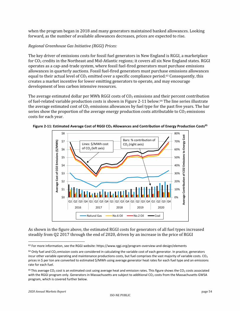
2020 Annual Markets Report page 54 ISO-NE PUBLIC
when the program began in 2018 and many generators maintained banked allowances. Looking forward, as the number of available allowances decreases, prices are expected to rise.
Regional Greenhouse Gas Initiative (RGGI) Prices:
The key driver of emissions costs for fossil fuel generators in New England is RGGI, a marketplace for CO2 credits in the Northeast and Mid-Atlantic regions; it covers all six New England states. RGGI operates as a cap-and-trade system, where fossil fuel-fired generators must purchase emissions allowances in quarterly auctions. Fossil fuel-fired generators must purchase emissions allowances equal to their actual level of CO2 emitted over a specific compliance period.63 Consequently, this creates a market incentive for lower emitting generators to operate, and may encourage development of less carbon intensive resources.
The average estimated dollar per MWh RGGI costs of CO2 emissions and their percent contribution of fuel-related variable production costs is shown in Figure 2-11 below.64 The line series illustrate the average estimated cost of C02 emissions allowances by fuel type for the past five years. The bar series show the proportion of the average energy production costs attributable to CO2 emissions costs for each year.
Figure 2-11: Estimated Average Cost of RGGI CO2 Allowances and Contribution of Energy Production Costs65
As shown in the figure above, the estimated RGGI costs for generators of all fuel types increased steadily from Q2 2017 through the end of 2020, driven by an increase in the price of RGGI
63 For more information, see the RGGI website: https://www.rggi.org/program-overview-and-design/elements
64 Only fuel and CO2 emission costs are considered in calculating the variable cost of each generator. In practice, generators incur other variable operating and maintenance productions costs, but fuel comprises the vast majority of variable costs. CO2 prices in $ per ton are converted to estimated $/MWh using average generator heat rates for each fuel type and an emissions rate for each fuel.
65 This average CO2 cost is an estimated cost using average heat and emission rates. This figure shows the CO2 costs associated with the RGGI program only. Generators in Massachusetts are subject to additional CO2 costs from the Massachusetts GWSA program, which is covered further below.
0%
10%
20%
30%
40%
50%
60%
70%
80%
$0
$1
$2
$3
$4
$5
$6
$7
$8
Q1 Q2 Q3 Q4 Q1 Q2 Q3 Q4 Q1 Q2 Q3 Q4 Q1 Q2 Q3 Q4 Q1 Q2 Q3 Q4
2016 2017 2018 2019 2020
Ave
rage
Co
ntr
ibu
tio
n o
f C
O2
Em
issi
on
s to
En
erg
y C
ost
Ave
rage
Co
st o
f C
O2
Em
issi
on
s ($
/MW
h)
Natural Gas No.6 Oil No.2 Oil Coal
Lines: $/MWh cost of CO2 (left axis)
Bars: % contribution of CO2 (right axis)

2020 Annual Markets Report page 55 ISO-NE PUBLIC
allowances. During Q2 2017, prices dropped to a daily low of $2.55/short ton, equating to $1.29/MWh for a standard natural gas-fired generator.66 However, prices increased 40% from $3.30/short ton to $4.60/short ton on August 23, 2017 after a RGGI program review placed a 30% reduction on the cap by 2030, relative to 2020 levels (from 78.2 million short tons to 54.7 million short tons).67,68
RGGI allowance prices increased by 15% in 2020 (from $5.51/short ton in 2019 to $6.31/short ton in 2020). For a typical natural gas-fired generator the average estimated CO2 cost was $2.88/MWh in 2020, an increase of $0.37/MWh from 2019. Several factors led to the increase in the price of RGGI allowances. As the fourth compliance period ended in 2020, RGGI participants sought additional allowances in auctions and secondary markets ahead of the fifth compliance deadline and the next RGGI program review in 2021.69 The number of market participants increased as New Jersey rejoined RGGI in 2020. Some generators in Virginia were also able to take part in 2020 markets ahead of their 2021 introduction to the program.70
The bars in Figure 2-11 show the relative contribution of RGGI CO2 emissions allowance costs to generator energy costs. This contribution increased for all fuel types in 2020. In Q3, the contribution of emissions to the energy cost of natural gas-fired generators reached 19.7%, which was the highest value over the five-year period. This was due to decreased natural gas prices and increased CO2 emissions prices.
A wider view of the impact of RGGI CO2 allowances on generator production costs is presented in Figure 2-12 below. The line series in the figure illustrate the quarterly estimated production costs using the average heat rate for generators of a representative technology type in each fuel category. The height of the shaded band above each line series represents the average energy production costs attributable to CO2 emissions costs in each quarter.
66 A standard natural gas-fired generator assumes a 7.8 MMBtu/MWh heat rate.
67 RGGI Inc. RGGI States Announce Proposed Program Changes: Additional 30% Emissions Cap Decline by 2030 August, 2017.
https://www.rggi.org/sites/default/files/Uploads/Program-Review/8-23-2017/Announcement_Proposed_Program_Changes.pdf
68 https://www.rggi.org/sites/default/files/Uploads/Program-Review/12-19-2017/Principles_Accompanying_Model_Rule.pdf
69 https://www.rggi.org/allowance-tracking/compliance
70 See https://www.rggi.org/sites/default/files/Uploads/Market-Monitor/Quarterly-Reports/MM_Secondary_Market_Report_2020_Q3.pdf

2020 Annual Markets Report page 56 ISO-NE PUBLIC
Figure 2-12: Contributions of Emissions Cost to Energy Production Costs
Figure 2-12 highlights that CO2 allowance costs have a relatively small impact on generator production costs and consequently do not have a noticeable impact on the economic merit order of generators.
Massachusetts Global Warming Solutions Act (MA GWSA) Prices:
In January 2018, Massachusetts implemented a new CO2 cap-and-trade program.71 The MA GWSA program provides additional requirements to the RGGI program discussed above, thus generators located in Massachusetts must meet both requirements. Administered by the Massachusetts Department of Environmental Protection (MassDEP), the program places an annual cap on aggregate CO2 production for the majority of fossil fuel-fired generators within the state.72 The cap will be lowered every year until the target annual CO2 emission rate is reached in 2050.73 To ensure compliance, the regulation requires fossil fuel-fired generators to hold an allowance for each metric ton of CO2 they produce during a year. For the first two years, these allowances were primarily allocated based on historical emissions levels, but beginning in 2021, allowances will be available for sale through auction only.74 The program allows generators to trade emissions allowances to meet their quotas.
To begin the program, the MassDEP allocated allowances based on historical emissions levels. Consequently, the market value of an allowance was unknown and the IMM calculated an opportunity cost-based adder for each facility using historical data to estimate the potential net revenue associated with each metric ton of CO2 output (i.e., the profit associated with each
71 310 CMR 7.74: Reducing CO2 Emissions from Electricity Generating Facilities (https://www.mass.gov/guides/electricity-generator-emissions-limits-310-cmr-774)
72 Participating generators are fossil-fuel generators with a nameplate capacity of 25 MW or more. See https://www.mass.gov/doc/310-cmr-700-air-pollution-control-regulations/download
73 The annual emissions cap for 310 CMR 7.74 will reduce by 223,876 metric tons in each subsequent year, eventually reaching 1,791,019 metric tons in 2050.
74 For the 2018, 2019, and 2020 compliance years, 100, 75, and 50 percent of emissions cap was directly allocated by MassDEP. MassDEP will no longer distribute allowances through direct allocation starting 2021.
$0
$20
$40
$60
$80
$100
$120
$140
$160
$180
$200
Q1 Q2 Q3 Q4 Q1 Q2 Q3 Q4 Q1 Q2 Q3 Q4 Q1 Q2 Q3 Q4 Q1 Q2 Q3 Q4
2016 2017 2018 2019 2020
Ene
rgy
Co
sts
($/M
Wh
)
Coal No.6 Oil No.2 Oil Natural Gas
Shaded area represents the cost of emissions
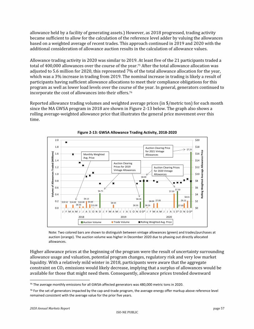
2020 Annual Markets Report page 57 ISO-NE PUBLIC
allowance held by a facility of generating assets.) However, as 2018 progressed, trading activity became sufficient to allow for the calculation of the reference level adder by valuing the allowances based on a weighted average of recent trades. This approach continued in 2019 and 2020 with the additional consideration of allowance auction results in the calculation of allowance values.
Allowance trading activity in 2020 was similar to 2019. At least five of the 21 participants traded a total of 400,000 allowances over the course of the year.75 After the total allowance allocation was adjusted to 5.6 million for 2020, this represented 7% of the total allowance allocation for the year, which was a 3% increase in trading from 2019. The nominal increase in trading is likely a result of participants having sufficient allowance allocations to meet their compliance obligations for this program as well as lower load levels over the course of the year. In general, generators continued to incorporate the cost of allowances into their offers.76
Reported allowance trading volumes and weighted average prices (in $/metric ton) for each month since the MA GWSA program in 2018 are shown in Figure 2-13 below. The graph also shows a rolling average-weighted allowance price that illustrates the general price movement over this time.
Figure 2-13: GWSA Allowance Trading Activity, 2018-2020
Note: Two colored bars are shown to distinguish between vintage allowances (green) and trades/purchases at auction (orange). The auction volume was higher in December 2020 due to phasing out directly allocated allowances.
Higher allowance prices at the beginning of the program were the result of uncertainty surrounding allowance usage and valuation, potential program changes, regulatory risk and very low market liquidity. With a relatively mild winter in 2018, participants were aware that the aggregate constraint on CO2 emissions would likely decrease, implying that a surplus of allowances would be available for those that might need them. Consequently, allowance prices trended downward
75 The average monthly emissions for all GWSA-affected generators was 480,000 metric tons in 2020.
76 For the set of generators impacted by the cap-and-trade program, the average energy offer markup above reference level remained consistent with the average value for the prior five years.
$19.52 $14.00$8.50
$10.00
$9.13
$9.69
$15.00
$6.71
$8.50$8.50
$8.26
$8.00
$8.26
$8.00 $7.00
$7.50$7.50
$7.00
$9.15
$8.01
$7.25
$0
$2
$4
$6
$8
$10
$12
$14
$16
$18
$20
0.0
0.2
0.4
0.6
0.8
1.0
1.2
1.4
1.6
1.8
2.0
J F M A M J J A S O N D J F M A M J J A S O N D D* J F M A M J J A S S* O N D D*
2018 2019 2020
Ro
llin
g W
eig
hte
d A
vera
ge A
llow
ance
Pri
ce
Vo
lum
e o
f A
llow
ance
s Tr
ade
d (
Mill
ion
s)
Trade Volume Rolling Weighted Avg. PriceAuction Volume
Monthly Weighted Avg. Price
Auction ClearingPrices for 2019 Vintage Allowances
Auction Clearing Prices for 2020 Vintage Allowances
Auction Clearing Price for 2021 Vintage Allowances

2020 Annual Markets Report page 58 ISO-NE PUBLIC
towards the end of the year. For 2019, the monthly-weighted average prices remained in the range of $7-$8/metric ton largely as a result of continued mild weather. The third year of the program (2020) marked the final year of directly allocated allowances by MassDEP. In subsequent compliance years, all allowances will be distributed through sale at auction. For 2020, prices ranged from $7-$9/metric ton. These prices reflected a surplus of allowances and relatively mild weather. However, as the number of available allowances decreases, prices are expected to rise. If the volume of transactions remains low, participants may find it difficult to obtain additional allowances without paying significant premiums.77 2.2.3 Generator Profitability
New generator owners rely on a combination of net revenue from energy and ancillary service markets and forward capacity payments to cover their fixed costs. Revenue from the Forward Capacity Market (FCM), which is conducted three-plus years in advance of the delivery year, is a critical component of moving forward with the development of a new project. Given the cost of a new project (CONE, or cost of new entry), developer expectations for minimum capacity revenues will be based on this cost and their expectation for net revenue from the energy and ancillary services markets. In New England, the majority of revenue to support new entry comes from the capacity market. There is an inverse relationship between expected net revenue from energy and ancillary service sales and the amount of revenue required from the capacity market in order to support new entry. As expected net revenue from energy and ancillary service sales decrease, more revenue is required from the capacity market to support new entry. The reverse is also true.
This section presents estimates of the net revenues that hypothetical new gas-fired generators (combined cycle (CC) and combustion turbine (CT)) could have earned in the energy and ancillary services markets in each of the previous five years. In addition to providing a basis for the amount of revenue required from the capacity market to build a new generator, this section also highlights the incremental revenue that could be earned from dual-fuel capability and evaluates participation in the Forward Reserve Market (FRM) for a combustion turbine generator.
The analysis is based on simulations of generator scheduling under an objective that maximizes net revenue while enforcing operational constraints, i.e., ramp rates, minimum run and down times, and economic limits.78 This year, the simulation model has been updated to explicitly include a Regional Greenhouse Gas Initiative (RGGI) cost for every short ton of CO2 emitted. In the model, the RGGI cost for each year is the average auction clearing price for RGGI allowances in that year.79
Figure 2-14 shows the result of the simulations.80 Each stacked bar represents revenue components for a generator type and year. A combined cycle generator is shown in green and a combustion turbine generator that participates in the FRM market is shown in blue. The simulation produces base revenue (energy and ancillary services (AS)) and incremental dual-fuel revenue numbers for
77 https://www.mass.gov/doc/market-monitor-quarterly-report-2020-q3/download.
78 The simulation uses historical market prices, which implies that the generator’s dispatch decisions do not have an impact on day-ahead or real-time energy prices. Results should be considered in the high range for potential revenue estimates because this analysis does not account for forced outages (which should be infrequent for a new generator).
79 RGGI Auction data is available at https://www.rggi.org/auctions/auction-results/prices-volumes.
80 The Gross CONE figures for the CC and CT gas-fired generators reflect Net CONE values of $9.00/kW-month and $7.23/kW-month with the difference between gross and net figures attributed to net revenue from energy and ancillary service sales.

2020 Annual Markets Report page 59 ISO-NE PUBLIC
2016-2020.81 Estimates of future year’s base revenue, dual-fuel revenue, and FRM revenue are simple averages of these numbers. For all years, the FCA revenue numbers shown are calculated using the actual payment rates applied to calendar years.
Figure 2-14: Estimated Net Revenue for New Gas-fired Generators
When compared with 2019, the simulation results show 2020 net revenues decreased by approximately 24% for the combined cycle generators and approximately 23% for the combustion turbines. The year-over-year decreases are a reflection of lower energy prices that resulted from generally milder weather and benign system conditions in 2020. Dual-fuel generators are especially impacted under these conditions because oil-burning capability offers no advantage when natural gas remains relatively inexpensive. Consequently, dual-fuel capability did not add any revenue for either CCGT or CT generators in 2019 or 2020. The drop in revenues is also partially explained by RGGI allowance auction prices which increased by 18% from the prior year.82 In addition, as energy prices decrease, RGGI costs become a higher share of the total cost of generation and have a greater impact on the frequency of intervals when it is economic for a generator to produce electricity. In other words, net revenue becomes more sensitive to RGGI costs as energy prices decrease.
Overall, the results show that if future market conditions remain similar to the previous five years, owners of new gas-fired combined cycle generators could expect net revenues (not including capacity payments) to average $3.44/kW-month which increases to $3.66/kW-month for generators with dual-fuel capability. Under the same conditions, new combustion turbines could expect net revenue earnings from $2.61/kW-month for single-fuel generators to $2.73/kW-month for generators with dual-fuel flexibility. With higher capacity factors, combined cycle generators can benefit more often from dual-fuel capability than peaking CT generators, but both technologies
81 Incremental dual-fuel energy revenue is earned by the generator when running on its second fuel type.
82 For this study RGGI auction prices were used to estimate average RGGI allowance costs. Under this approach, RGGI allowances increased by 18% from 2019. An alternative approach is to use daily index values for RGGI allowances that are derived from trading activity. This is the approach that is used in Carbon Emissions Markets section of this document which reported a year-over-year increase of 15% in RGGI costs.
2016 2017 2018 2019 2020 2021 2022 2023
$0
$5
$10
$15
$20$
/kW
-mo
Series7 Axis
CT Gross CONE (FCA15) = $10.40
CC Gross CONE (FCA15) = $14.32
Future Periods
Base revenue Incremental dual-fuel FRM revenue FCA revenue
Combined CycleCombustion Turbine

2020 Annual Markets Report page 60 ISO-NE PUBLIC
can expect significant revenue gains when gas prices rise above oil prices as occurred in the winter of 2018.
A combustion turbine generator can also participate in the Forward Reserve Market (FRM) where off-line reserves are procured prior to the reserve season. A forward reserve resource receives revenue from the forward reserve auction, but it foregoes real-time reserve payments and, in most hours where the energy price is within a normal range, also foregoes energy revenue since it will be held in reserve. When the energy price is very high, as in the case of a scarcity event, the forward reserve resource may be dispatched for energy and would then receive net revenue (above variable cost) for those high-priced periods. While FRM auction payments have trended lower recently, this analysis shows that a new combustion turbine that is designated as an FRM resource could earn $0.58/kW-month more net revenue than the same resource could have accumulated in the real-time market alone. In addition, participation in the FRM market results in greater net revenue than non-participation in all five years where these revenues have been observed (not future periods). Note, however, that the profitability of FRM participation is particularly sensitive to the frequency of scarcity pricing events via the Reserve-Constraint Penalty Factor (RCPF).
The simulations show that average revenues for new gas-fired generators appear to be lower than benchmark estimates used to establish CONE numbers for the Forward Capacity Auctions (FCAs). The most recent CONE revisions approved by FERC establish net revenue components of $5.32/kW-month and $3.17/kW-month for combined cycle and combustion turbine generators respectively.83 However, even revenue numbers in this range are clearly insufficient to support new entry without the addition of capacity payments to cover the fixed costs of a new gas-fired generator.
In recent years, capacity prices have trended downwards reflecting a system that is increasingly long on capacity. Total revenues from the energy and capacity markets appear insufficient to support new entry from combined cycle generators and would likely only incent the most efficient of combustion turbines to enter the region’s energy market. While two recent FCAS (FCA 12 and FCA 13) each had entry by one new gas–fired generator, no new gas-fired generation cleared in the two most recent auctions (FCA 14 and FCA 15).
Note that CONE benchmarks are produced from financial and engineering studies that estimate the cost of adding green-field generators. In practice, the cost of new entry for a generator may be lower than the current CONE benchmarks for a number of reasons. In particular, when new generating units are built on existing generation sites or when there are material additions to the capacity of an existing operational plant, the presence of existing infrastructure tends to lower fixed costs.
2.2.4 Energy Demand
In 2020, New England wholesale electricity load decreased by 2.3%, leading to record low loads. Temperature fluctuations typically drive yearly differences in wholesale load, but wholesale load in New England has continually decreased in most recent years due to increased energy efficiency and behind-the-meter solar generation. In 2020, the COVID-19 pandemic also contributed to lower loads, on average. On a weather-normalized basis, wholesale load decreased by 2.4% compared to 2019. The similar change in load and weather-normalized load shows that energy efficiency, behind-the-meter solar generation and the COVID-19 pandemic explain most of the annual decline
83 These revenue components include “Pay-for-Performance” (PFP) revenue which this study does not.

2020 Annual Markets Report page 61 ISO-NE PUBLIC
in average load. We estimate that the COVID-19 pandemic contributed about 0.5% (or about a quarter) to the overall 2% overall decline in load.
Quarterly average load from 2016 to 2020 is shown in Figure 2-15 below. The solid black lines show quarterly average load and the dashed black lines represent annual average load. The different colored dots identify each calendar quarter (Q1 – blue, Q2 – green, Q3 – red, Q4 – yellow).
Figure 2-15: Average Hourly Load by Quarter and Year
In 2020, quarterly average load decreased in all quarters except for Q3 (summer) when compared to 2019. In Q1 2020 average load decreased by 6.0% (850 MW) year-over-year due to warmer temperatures. Temperatures averaged 36⁰F, a 5⁰F increase compared to Q1 2019 (31⁰F) and the warmest Q1 over the last five years. Beginning in March 2020, state-wide closures were implemented to mitigate the spread of COVID-19, which generally led to decreased electricity demand. The COVID-19 pandemic continued to reduce average loads during Q2 2020. In Q2, quarterly average load decreased by 1.5% (184 MW) despite increased heating degree days (HDD) and cooling degree days (CDD).84 Compared to Q2 2019, HDDs increased by 162 and CDDs increased by 79, which suggests loads may have otherwise increased during normal economic conditions.85
In Q3, quarterly average load increased by 0.8% (125 MW) due to warmer weather and increased air-conditioning demand due to the COVID-19 pandemic, which resulted in wider dependence on less efficient residential systems as many people remained at home.86 In Q3 2020 the Temperature-
84 Heating degree day (HDD) measures how cold an average daily temperature is relative to 65°F and is an indicator of electricity demand for heating. It is calculated as the number of degrees (°F) that each day’s average temperature is below 65°F. For example, if a day’s average temperature is 60°F, the HDD for that day is five. Cooling degree day (CDD) measures how warm an average daily temperature is relative to 65°F and is an indicator of electricity demand for air conditioning. It is calculated as the number of degrees (°F) that each day’s average temperature is above 65°F. For example, if a day’s average temperature is 70°F, the CDD for that day is five.
85 Loads may have increased under normal conditions before factoring in the long-term trends like energy efficiency and behind-the-meter solar.
86 For more information, see the ISO’s weekly Estimated Impacts of COVID-19 on Demand
10,000
11,000
12,000
13,000
14,000
15,000
16,000
17,000
18,000
1 2 3 4 1 2 3 4 1 2 3 4 1 2 3 4 1 2 3 4
2016 2017 2018 2019 2020
MW
Annual Average Load
Quarterly Average Load

2020 Annual Markets Report page 62 ISO-NE PUBLIC
Humidity Index (THI) averaged a 68.4, a 0.3 increase compared to Q3 2020. Average Q4 load decreased by 2.6% (345 MW) year-over-year, due to milder weather. HDDs decreased compared to Q4 2019 (1,867 from 2,098), leading to less electricity demand.
New England’s system load over the last five years is shown as load duration curves in Figure 2-16 below. A load duration curve depicts the relationship between load levels and the frequency that load levels occur. The red line shows 2020 and the range of gray lines (from lightest to darkest) show 2016-2019. The inset graph highlights the 5% of hours with the highest load levels for each year.
Figure 2-16: Load Duration Curves
The 2020 load duration curve was lower compared to 2016 – 2019 in 93% of all hours. This highlights the long-term trend of decreasing wholesale load due to increases in energy efficiency and behind-the-meter solar generation. The 7% of hours during 2020 with higher loads mostly occurred during in July and August when hot weather increased air-conditioning demand. The inset graph highlights the load duration curves during the top 5% load levels during the year. These hours tend to occur during the summer when increased air-conditioning demand drives higher wholesale electricity demand. Therefore, weather differences tend to explain annual variations during the top 5% of hours. In 2020, the top 5% of load levels were higher than in 2017 and 2019, but lower than most hours in 2016 and all hours in 2018. In Summer 2020 (Q3) temperatures averaged 71.2⁰F, warmer than in 2017 (69.3⁰F) and 2019 (70.9⁰F) but cooler than in 2016 (71.9⁰F) and 2018 (72.0⁰F). As mentioned above, the restriction associated with the COVID-19 pandemic also caused increased residential air-conditioning demand during the summer. While actual average load decreased by 2.3%, weather-normalized load only declined by 2.4% relative to 2019.87 Average annual weather-normalized load has fallen every year since 2011 due to growth in energy efficiency and, to a lesser extent, behind-the-meter solar generation. Figure 2-17
87 Weather-normalized load adjusts observed load for the effects of weather, leap year and non-holiday weekdays.
8,000
10,000
12,000
14,000
16,000
18,000
20,000
22,000
24,000
26,000
28,000
0% 20% 40% 60% 80% 100%
Ho
url
y Lo
ad (
MW
)
2016 2017 2018 2019 2020

2020 Annual Markets Report page 63 ISO-NE PUBLIC
displays the average quarterly weather-normalized load and the estimated impact of energy efficiency and behind-the-meter solar over the past five years.88
Figure 2-17: Average Quarterly Weather-Normalized Load with Energy Efficiency and Solar Impacts
Weather-normalized net load (solid blue line in Figure 2-17) fluctuates from quarter to quarter but has trended downward over the past five years. Weather normalized gross load (dashed purple line), which shows load without the effects of energy efficiency and behind-the-meter solar, has grown slightly since 2016. The gap between weather-normalized gross load and actual load is the combined impact of energy efficiency (green area) and behind-the-meter solar generation (gold area). Greater energy efficiency and behind-the-meter solar generation have helped offset the increase in gross load, causing weather-normalized load to fall. In 2020, energy efficiency reduced annual average load by an estimated 2,433 MW, a 7% increase (156 MW) compared to 2019, and a 43% increase (737 MW) compared to 2016. Behind-the-meter solar generation reduced annual average load by 338 MW or nearly 14% of estimated installed capacity (2,431 MW). The 338 MW average load reduction was an 18% increase (51 MW) compared to 2019. While the effect of behind-the-meter solar generation is less than that of energy efficiency, behind-the-meter solar generation has grown more rapidly, increasing 104% (172 MW per hour) compared to 2016. By 2029, behind-the-meter solar generation is expected to reduce annual load by an average of 632 MW.89 Energy efficiency and behind-the-meter solar generation impact wholesale load differently during the year. Figure 2-17 shows that energy efficiency has a greater effect during Q1 and Q4, while behind-the-meter solar generation has a greater impact during Q2 and Q3.
88 Energy Efficiency is based on aggregated performance of installed measures on end-use customer facilities that reduce the total amount of electrical energy needed, while delivering a comparable or improved level of end-use service. Such measures include, but are not limited to, the installation of more energy efficient lighting, motors, refrigeration, HVAC equipment and control systems, envelope measures, operations and maintenance procedures, and industrial process equipment. Energy Efficiency and Demand Response Distributed Generation (DG) measures are aggregated to On-Peak and Seasonal-Peak resources. Performance of DG accounts for only 5% of energy efficiency performance.
89 For more information, see ISO New England’s CELT Report.
0
1,000
2,000
3,000
4,000
5,000
6,000
7,000
8,000
9,000
10,000
8,000
9,000
10,000
11,000
12,000
13,000
14,000
15,000
16,000
17,000
18,000
1 2 3 4 1 2 3 4 1 2 3 4 1 2 3 4 1 2 3 4
2016 2017 2018 2019 2020
Ene
rgy
Effi
cie
ncy
& S
ola
rIm
pac
ts (
MW
)
MW
Energy Efficiency Behind-the-Meter Solar
Weather-Normalized Net Load Weather-Normalized Gross Load
Weather-normalized load has declined...
Trendlines for Gross Load, Net Load, and EE+ Solar
...as energy efficiency and solar have grown.

2020 Annual Markets Report page 64 ISO-NE PUBLIC
2.2.5 Reserve Requirements
Bulk power systems need reserve capacity to respond to contingencies. ISO New England’s reserve requirements are designed to allow the bulk power system to serve load uninterrupted if there is a loss of a major generator or transmission line.90 The first level requirement is for the ISO to maintain a sufficient amount of reserves to be able to recover from the loss of the largest single system contingency (N-1) within 10 minutes. This requirement is referred to as the total 10-minute reserve requirement. At least 25% of the total 10-minute reserve requirement must be synchronized to the power system. The exact amount is determined by the system operators, and this amount is referred to as the 10-minute spinning reserve (TMSR) requirement. The rest of the total 10-minute reserve requirement can be met by 10-minute non-spinning reserve (TMNSR).
Additionally, adequate operating reserves must be available within 30 minutes to meet 50% of the second-largest system contingency (N-1-1). This requirement can be satisfied by thirty-minute operating reserves (TMOR). Starting in October 2013, the ISO added a thirty-minute replacement reserve requirement of 160 MW for the summer and 180 MW for the winter months.91 Adding these additional requirements to the total 10-minute reserve requirement comprises the system total reserve requirement (the green bar below).
In addition to the system-wide requirements, 30-minute reserves must be available to meet the local second contingency in import-constrained areas. Local TMOR requirements exist for the region’s three local reserve zones – Connecticut, Southwest Connecticut (SWCT), and NEMA/Boston. Local reserve requirements reflect the need for 30-minute contingency response to provide second contingency protection for each import-constrained reserve zone. Local reserve requirements can be satisfied by resources located within a local reserve zone or through external reserve support. Average annual local reserve requirements are shown in the right panel of Figure 2-18 below. Note in the left graph that the bars showing the total 10 requirement (purple) includes both spinning and non-spinning 10-minutes reserves, while the total 30 requirement (green) includes the total 10-minute and 30-minute requirements.
90 Operating Procedure No. 8, Operating Reserves and Regulation (August 2, 2019), https://www.iso-ne.com/static-assets/documents/rules_proceds/operating/isone/op8/op8_rto_final.pdf
91 Operating Procedure No. 8 states that in addition to the operating reserve requirements, ISO will maintain a quantity of Replacement Reserves in the form of additional TMOR for the purposes of meeting the NERC requirement to restore its Ten-Minute Reserve. ISO will not activate emergency procedures, such as OP-4 or ISO New England Operating Procedures No. 7 - Action in an Emergency (OP-7), in order to maintain the Replacement Reserve Requirement. To the extent that, in the judgment of the ISO New England Chief Operating Officer or an authorized designee, the New England RCA/BAA can be operated within NERC, NPCC, and ISO established criteria, the Replacement Reserve Requirement may be decreased to zero based upon ISO capability to restore Ten-Minute Reserve within NERC requirements.

2020 Annual Markets Report page 65 ISO-NE PUBLIC
Figure 2-18: Average System Reserve and Local 30-Minute Reserve Requirements
The average 10-minute spinning requirement was 527 MW in 2019 and 2020, which was lower than in previous years. The requirement is calculated as a percentage of the total 10-minute requirement. In June 2018, the average spinning reserve requirement fell from 37% to 31% of the total 10-minute requirement. The decline was driven by market operation studies that suggested changes in generator performance required fewer spinning reserves to be online at any given time. Over the past five years, total 10-minute and total 30 reserve requirements have averaged around 1,700 MW and 2,500 MW, respectively. The requirements are primarily determined by the size of the first and second largest contingencies on the system, so the average annual requirements tend not to fluctuate substantially from year to year.
The largest change to average requirements was in the Southwest CT (SWCT) reserve zone. The average requirement increased 21% from 848 MW in 2019 to 1,025 MW in 2020. Over the same period, SWCT went from exporting 73 MW of energy per hour in 2019, to importing 190 MW of energy per hour, on average, in 2020. This change reduced the ability of the transmission system to provide external reserve support, which meant the local reserve requirement needed to be higher on average. Despite the decline in the SWCT requirement, there were zero intervals with local thirty-minute operating reserve prices in SWCT for the second year in a row. Reserve pricing is discussed in more detail in Section 7.1
2.2.6 Capacity Market Requirements
The Installed Capacity Requirement (ICR) is the amount of capacity (expressed in megawatts) needed to meet the region’s reliability requirements (including energy and reserves). The ICR requirements are designed such that non-interruptible customers can expect to have their load curtailed not more than one day every ten years.92
When developing the target capacity to be procured in the Forward Capacity Auction (FCA), the ISO utilizes a Net ICR. The Net Installed Capacity Requirement (NICR) is the amount of capacity needed to meet the region’s reliability requirements after accounting for tie benefits with Hydro-Quebec.93
92 The ISO develops the ICR through a stakeholder and regulatory process with review and action by various NEPOOL committees, state regulators, and the New England States Committee on Electricity.
93 The HQ tie-benefit in FCA 15 was about 900 MW. There is no CSO associated with this, unlike with other import resources.
-
500
1,000
1,500
2,000
2,500
3,000
2016 2017 2018 2019 2020
Res
erve
Req
uir
emen
t (M
W)
System
10 Spin Requirement Total 10 Requirement Total 30 Requirement
-
500
1,000
1,500
2,000
2,500
3,000
2016 2017 2018 2019 2020
Local
Connecticut NEMA/Boston Southwest CT

2020 Annual Markets Report page 66 ISO-NE PUBLIC
Due to transmission limitations there are also local sourcing requirements (LSR) for import-constrained areas and maximum capacity limits (MCL) for export-constrained areas.
Trends in system capacity requirements, ICR and Net ICR, between 2017 and 2025 are shown in Figure 2-19 below. The system ICR and Net ICR are represented as line series. LSRs (positive bars) and MCLs (negative bars) are also shown.
Figure 2-19: ICR, NICR, Local Sourcing Requirements, and Maximum Capacity Limits
The Net Installed Capacity Requirement for FCA 15 (2024-25 delivery period) was 33,270 MW. The Net ICR increased by 780 MW, or by 3%, from FCA 14, primarily due to the introduction of transportation and heating electrification to peak load forecasts and decreased interchange tie benefits.
Local Sourcing Requirements (LSRs) are placed on import-constrained zones due to limited import capability and potential reliance on local generation to meet local load and reserve requirements. As zonal capacity approaches and falls below the LSR, additional capacity within the zone becomes increasingly valuable due to declining reliability in the local area. Starting in FCA 10, Southeast New England (SENE) was the only import-constrained zone, and Connecticut and NEMA/Boston were no longer import-constrained due to improvements to the transmission system.94 In FCA 15 the LSR in SENE increased to 10,305 MW, 550 MW higher than FCA 14 (9,757 MW), due to a significant increase in the Local Resource Adequacy (LRA) requirement for SENE.95
Maximum capacity limits (MCLs) are placed on export-constrained zones due to limited export capability. These zones may procure more generation capability than can be exported to the rest of the system. Surplus capacity within the export-constrained zone becomes decreasingly valuable due to its declining contribution to system reliability. The Maine and Northern New England (NNE) capacity zones were modeled as separate export-constrained capacity zones for both FCA 14 and
94 Southeast New England consists of the NEMA/Boston, Southeastern Massachusetts, and Rhode Island load zones.
95 The Local Resource Adequacy requirement represents the minimum amount of capacity in a zone needed to meet system-wide reliability requirements.
(15,000)
(10,000)
(5,000)
0
5,000
10,000
15,000
20,000
25,000
30,000
35,000
40,000
8 9 10 11 12 13 14 15
2017-18 2018-19 2019-20 2020-21 2021-22 2022-23 2023-24 2024-25
MW
Forward Capacity Auction Number (Commitment Period)
Connecticut NEMA/Boston SEMA/RISoutheast New England Maine Northern New EnglandNet ICR ICR
Future Periods

2020 Annual Markets Report page 67 ISO-NE PUBLIC
FCA 15, after applying the updated nested capacity methodology.96 In FCA 15, the MCLs were 4,145 MW in Maine, and 8,680 MW in Northern New England; which includes Maine, Vermont, and New Hampshire.
2.3 Imports and Exports (External Transactions)
New England engages in the buying and selling of power with its neighboring control areas of New York, Hydro Québec, and New Brunswick over the transmission lines that interconnect the regions. External transactions allow competitive wholesale markets to deliver load at a lower cost by displacing more-expensive native generation when imported power is available. Generators in exporting ISOs also benefit when there is no willing buyer of their power in their region, but there are customers willing to purchase their energy in another region.
External transactions allow participants to purchase power in one region, and sell power in another, in the day-ahead and real-time markets, with the goal of profiting from the difference in energy prices (or price spread) between the two regions. The ISO schedules these transactions and coordinates the interface power flow with neighboring areas based on the transactions that have been cleared and confirmed. The energy price produced by ISO-NE for an interface represents the value of energy at the location in the New England market, not in the neighboring area. The ISO-NE market settles the part of the transaction that occurs in the New England market; the neighboring control area settles the corresponding transaction on the other side of the interface.
Market participants can also use external transactions to fulfill other contractual obligations to buy or sell power (e.g., a power purchase agreement) or to import and collect credits for renewable power. Participants submit external transactions to specific locations known as external nodes, which are affiliated with specific external interfaces. The nodes represent trading and pricing points for a specific neighboring area. A pricing node may correspond to one or more transmission line(s) that connect the control areas.
New England’s six external nodes are listed in Table 2-1 below, along with the commonly used external interface name. These names will be used throughout this section. There are three interfaces with New York, two with Hydro Québec and one with New Brunswick. The table also lists each interface’s import and export total transfer capability (TTC) ratings. The operational ratings can be different for import and export capabilities at the same interface due to the impact of power transfers in each direction on reliability criteria.
96 See Market Rule 1, Section III.12.2.2 of the Tariff.

2020 Annual Markets Report page 68 ISO-NE PUBLIC
Table 2-1: External Interfaces and Transfer Capabilities
Neighboring area Interface name External node name Import
capability (MW) Export
capability (MW)
New York New York North .I.ROSETON 345 1 1,400 - 1,600 1,200
New York Northport-Norwalk Cable .I.NRTHPORT138 5 200 200
New York Cross Sound Cable .I.SHOREHAM138 99 346 330
Hydro Québec (Canada) Phase II .I.HQ_P1_P2345 5 2,000 1,200
Hydro Québec (Canada) Highgate .I.HQHIGATE 120 2 225 170
New Brunswick (Canada) New Brunswick .I.SALBRYNB345 1 1,000 550
Total 5,171 – 5,371 3,480-3,555
Net Interchange
The average hourly net interchange values from the day-ahead and real-time markets for 2016 through 2020 are shown in the line series of Figure 2-20 below. The figure also charts the hourly average imported volume (positive values) and exported volume (negative values) in the bar series. The real-time import and export volumes are shown as the incremental additions to the amounts cleared in the day-ahead market.
Figure 2-20: Hourly Average Day-Ahead and Real-Time Pool Net Interchange
New England continued to be a net importer of power in 2020; real-time net imports averaged 2,680 MW each hour, meeting 20% of New England’s wholesale electricity demand. Total net interchange was 2% higher than in 2019. In 2020 decreases in both imports (43 MW) and exports (91 MW), netted to a 47 MW increase in interchange (net imports), on average. The slight increase was driven by more net imports from New York.
New England imports significantly more power from the Canadian provinces than it does from New York. Across all three Canadian interfaces (i.e., Phase II, New Brunswick, and Highgate) the real-time net interchange averaged 1,876 MW per hour in 2020, which was 100 MW less than the average interchange in 2019. The real-time net interchange across the three interfaces with New
(1,000)
(500)
0
500
1,000
1,500
2,000
2,500
3,000
3,500
2016 2017 2018 2019 2020
Ho
url
y A
vera
ge M
W
Day-ahead imports Real-time imports
Day-ahead exports Real-time exports
Day-ahead net interchange Real-time net interchange

2020 Annual Markets Report page 69 ISO-NE PUBLIC
York (i.e., New York North, Cross Sound Cable and Northport-Norwalk) averaged 804 MW per hour in 2020, 148 MW more than the average 2019 net interchange. Section 5 of this report provides further detail on the breakdown of total external transactions among the various interfaces with New York and Canada.
The hourly average real-time net interchange increased every year between 2017 and 2020, as shown by the red line series. Real-time imports increased by 426 MW per hour (15%) from 2016 to 2020, on average. Similarly, real-time exports increased by 115 MW per hour (21%), on average, over the reporting period. The net increases occurred primarily at the New York North interface, where Coordinated Transaction Scheduling (CTS) went into effect on December 15, 2015. CTS was designed to improve the efficiency of energy transactions between New England and New York.
The close proximity of the day-ahead net interchange (orange) and real-time net interchange (red) line series highlights that day-ahead market outcomes across the external nodes do, on average, closely predict the real-time scheduled flows.97 Although additional import and export transactions are scheduled in real-time relative to day-ahead (shown by the darker colored bar series), the volumes of incremental real-time import and export schedules almost offset each other. Average real-time net interchange was greater than day-ahead net interchange by just 1.7% during 2020 (i.e., slightly more power was imported in real-time than planned for day-ahead). For the remainder of this section, only the real-time values are presented since they align so closely with day-ahead values.
Net Interchange by Quarter
The hourly average real-time pool net interchange value is plotted by quarter for 2016 through 2020 in Figure 2-21 below. Note that the observations are grouped by calendar quarter in the chart. Each quarter’s net interchange value is plotted with the red line series and, for comparison purposes, the five-year averages for each quarter are shown with the gray line series.
Figure 2-21: Hourly Average Real-Time Pool Net Interchange by Quarter
97 Virtual transactions cleared at external interfaces in the day-ahead market are included in the day-ahead net interchange value. In the day-ahead energy market, virtual supply and demand are treated as physical imports or exports.
0
500
1,000
1,500
2,000
2,500
3,000
3,500
20
16
20
17
20
18
20
19
20
20
20
16
20
17
20
18
20
19
20
20
20
16
20
17
20
18
20
19
20
20
20
16
20
17
20
18
20
19
20
20
Q1 Q2 Q3 Q4
Ho
url
y av
era
ge M
W
Real-time net interchange
5-year average for the quarter

2020 Annual Markets Report page 70 ISO-NE PUBLIC
As the quarterly-segmented plots in Figure 2-21 show, there is seasonal fluctuation in the system net interchange. The fluctuation is demonstrated by the movement in the five-year average lines (gray) from a high during late winter (i.e., Q1) when heating demand and natural gas-fired generators compete for constrained gas supplies, down to a low during the spring (i.e., Q2) when temperatures are moderate, and loads and natural gas prices are typically at their lowest levels. The average net interchange climbs during the summer (i.e., Q3) when New England loads are typically highest, and moves to a second peak at the start of winter (i.e., Q4) when heating demand once again begins to put upward pressure on natural gas and electricity prices. Fuel prices are discussed more in Section 2.2.2.
Relative to 2019, the 2020 quarterly average net interchange changed the most in the middle two quarters of the year. In Q2 2020, the average net interchange was 559 MW per hour more than in Q2 2019, due to an increase in imports and a decrease in exports over the New York North interface. The increase in imports over the New York North interface was driven by an increase in fixed and low-priced import offers, and not by differences in day-ahead and real-time prices between the markets. These fixed and low-priced offers may be due to contractual positions that participants enter into prior to the delivery day. New England imported less power in Q1 and Q3 2020 than in the same quarters in 2019. In Q3 2020, the average net interchange was 410 MW per hour less in Q3 2019. This decrease was due to a combination of fewer imports over the Phase II, New York North and New Brunswick interfaces and fewer exports over the Cross Sound Cable. The decrease over Phase II was due to a few planned transmission outages that lowered the import transfer capability. Similarly, the Cross Sound Cable’s transfer capability was lower for most of the second half of the year, decreasing exports. Lastly, bidding behavior over New Brunswick shifted to a more price sensitive pattern. This is discussed further in Section 5.1.

2020 Annual Markets Report page 71 ISO-NE PUBLIC
Section 3 Day-Ahead and Real-Time Energy Market
This section covers energy market outcomes, including the drivers of prices, market performance, competitiveness and market power mitigation.
The day-ahead and real-time energy markets are designed to ensure wholesale electricity is supplied at competitive prices, while maintaining the reliability of the power grid. Competitive energy market prices that reflect the underlying cost of electricity production are key to achieving both design goals. If suppliers can inflate prices above competitive levels, buyers will be forced to pay uncompetitive prices that exceed the cost of supplying power. On the other hand, if market prices are deflated (priced below production cost), suppliers lose the incentive to deliver power when it is needed. Further, investment in new, economically viable projects is hindered by deflated prices, hurting the short-term and long-term reliability of the New England power grid. Competitive energy market prices send the correct market signals, resulting in efficient buying and selling decisions that benefit consumers and suppliers alike.
In 2020, total day-ahead and real-time energy payments reflected changes in underlying primary fuel prices, most notably natural gas. The average Hub price was $23.32/MWh in the day-ahead market, down by 25% on 2019, and consistent with the 36% decrease in natural gas prices and with changes to the supply mix, most notably the decrease in fixed-priced nuclear supply and the corresponding increase in priced natural gas-fired generation.
Under certain system conditions, suppliers can have local or system-wide market power. If suppliers exploit market power opportunities by inflating energy offers, uncompetitive market prices can result. To diminish the impacts of market power, energy market mitigation measures are applied when market power is detected; an uncompetitive generator offer is replaced with an IMM calculated competitive offer (i.e. reference level) consistent with the generator’s cost of energy production.
Overall, day-ahead price-cost markups (i.e. the premium in market prices resulting from differences in generator offers and marginal costs) were within reason and market concentration levels, on average, remained reasonably low. Energy supply portfolios with structural market power in the real-time market remained low for the second consecutive year, declining from a third of hours in 2018, to 15% in 2019 and 17% in 2020. The reduction in the number of intervals with pivotal suppliers is consistent with a number of market trends, including a higher reserve surplus, and lack of scarcity conditions over the past two years, and the commissioning of new entrant generators.
The energy market has an extensive set of rules to identify and mitigate the impact of uncompetitive offers at times when structural market power exists. However, the mitigation measures for system-level market power in the real-time energy market provide suppliers a considerable degree of deviation from competitive marginal-cost offers before the mitigation rules trigger and mitigate a supply offer. Our analysis indicates that lower thresholds would not have had a significant impact on offer mitigation over the past few years since the market has generally been competitive, particularly due to surplus supply conditions. However, in our opinion, it is an appropriate time for the ISO to revisit and potentially lower the mitigation thresholds, which will strike a better balance between protecting consumers and administratively intervening in the market as the supply margin contracts in future years.

2020 Annual Markets Report page 72 ISO-NE PUBLIC
3.1 Overview of the Day-Ahead and Real-Time Energy Markets
This section provides an overview of the day-ahead and real-time energy markets.
ISO-NE administers its wholesale energy market using a two-settlement system. The first settlement takes place in the day-ahead energy market. This is a forward market where market participants buy and sell power for the following operating day. The day-ahead market is often considered a financial market because there is no physical requirement that the energy bought and sold in this market be consumed or delivered in real-time.98 The second settlement occurs in the real-time energy market. This is a spot market that coordinates the dispatch of resources in real-time based on actual conditions in the power system. The real-time market is a physical market because the transactions that occur in this market correspond to actual power flows.
As mentioned above, the day-ahead energy market allows participants to buy and sell electricity the day before the operating day. Participants that are interested in purchasing electricity can submit demand bids into the day-ahead energy market. These bids indicate the maximum price a buyer is willing to pay in order to purchase a certain quantity of electricity. Demand bids with bid prices greater than the locational marginal price (LMP) clear in the day-ahead market. Participants that are interested in selling electricity can submit supply offers into the day-ahead energy market.99 These offers indicate the minimum price the seller is willing to accept in order to sell a certain quantity of electricity. Supply offers with offer prices less than the LMP clear in the day-ahead market.
Clearing a demand bid or a supply offer in the day-ahead market results in an initial settlement (i.e., the day-ahead settlement) and creates a financial obligation for the buyer or seller. For example, a generator that clears a 100-MW supply offer in the day-ahead market at a price of $50/MWh would be credited $5,000 in the day-ahead settlement. This generator receives a payment because it has financially obligated itself to provide power in real-time on the following day. This obligation requires the generator to deliver in real-time every megawatt it sold forward or else purchase power at a replacement price; i.e. at the real-time price. Physical delivery in real-time results in the second settlement for the generator (i.e., the real-time settlement). For example, if the generator provides no energy in real-time and the real-time price of energy is $75/MWh, then the generator would be charged $7,500 in the real-time settlement. The net outcome from the two settlements would be a charge of $2,500 to the generator for not delivering on its obligation.
One of the primary reasons for this two-settlement design is that it affords participants a way to reduce their exposure to real-time energy price volatility. Unexpected events like transmission or generator outages can lead to very high real-time energy prices. However, buyers and sellers who bought or sold energy in the day-ahead market are not exposed to these extreme real-time prices so long as they do not deviate from their day-ahead market obligations. This is because real-time energy prices apply only to deviations from day-ahead market obligations.
For example, consider a load-serving entity (LSE) that purchases 100 MW of electricity in the day-ahead market at a price of $50/MWh. This purchase creates a charge to the LSE of $5,000 in the
98 However, the day-ahead market is not completely separated from the physical market as the commitments made in the day-ahead energy market form the basis of the operating plan that is used in real-time.
99 In general, resources with a capacity supply obligation (CSO) are required to submit supply offers into the day-ahead energy market of a magnitude at least equal to the megawatt amount of CSO they hold. The obligations associated with assuming a CSO create a linkage that ties the energy market to the capacity market, which is discussed in more detail in Section 6.

2020 Annual Markets Report page 73 ISO-NE PUBLIC
day-ahead settlement. If the real-time price is $75/MWh and the real-time load for the LSE is 110 MWs, then the real-time settlement would result in an additional charge of $750. This is because the real-time price only applies to the 10 MW deviation. The net outcome from the two settlements would be a charge of $5,750 to the LSE. If the LSE had not participated in the day-ahead market, then it would have been charged $75/MWh for all 110 MWs of its real-time load. This would have resulted in a charge of $8,250 to the LSE. Effectively, the LSE has partially insulated itself from the higher real-time prices by participating in the day-ahead market.
Because the day-ahead energy market is a financial market, participants may submit virtual demand bids (decrement bids) or virtual supply offers (incremental offers) into this market. As the name implies, virtual demand bids and supply offers are not expected to be backed by physical power. Collectively known as virtual transactions, these instruments allow participants to take financial positions in the day-ahead market with the expectation that the associated power will not be delivered or consumed in real-time. There are a number of arguments on how two-settlement markets, like ISO-NE’s wholesale energy market, benefit from virtual transactions. These include the ability of virtual transactions to reduce market power, the increased liquidity they provide to the day-ahead market, and their ability to improve price convergence. Virtual transactions are discussed in more detail in Section 4.
The day-ahead market purchases enough physical and virtual supply to meet physical and virtual demand.100 In order to determine which bids and offers clear, the day-ahead market uses a clearing algorithm with the objective of maximizing social surplus, while respecting transmission constraints. The day-ahead market results form the basis of the ISO Control Room’s operating plan for the following day. In the day-ahead market, virtual bids and offers can be submitted at a nodal level, zonal level or at the Hub.101 However, supply offers from generators must be submitted at the nodal location where that generator is electrically interconnected, and non-virtual demand bids are submitted at a zonal level. All results are hourly in the day-ahead market. The results are usually posted no later than 1:30 p.m. the day before the operating day.
The real-time energy market can be thought of as a “balancing market,” settling the differences between positions (production or consumption) cleared in the day-ahead energy market and actual production or consumption in the real-time energy market. The ISO coordinates the production of electricity to ensure that the amount produced moment to moment equals the amount consumed, while respecting transmission constraints. While resources continue to make supply offers in real-time, the demand is the actual physical load. In real-time, the ISO calculates LMPs every five minutes for each location on the transmission system at which power is either withdrawn or injected.
100 Operating reserves, described in Section 7.1, are not explicitly purchased through the day-ahead market. Operating reserves are procured in the Forward Reserve Market (see Section 7.2), and additional procurement occurs in the real-time energy market where reserve procurement is co-optimized with energy procurement.
101 The Hub, load zones, and internal network nodes are points on the New England transmission system at which locational marginal prices (LMPs) are calculated. Internal nodes are individual pricing points (pnodes) on the system. Load zones are aggregations of internal nodes within specific geographic areas. The Hub is a collection of internal nodes intended to represent an uncongested price for electric energy that is used to facilitate energy trading. The Hub LMP is calculated as a simple average of LMPs at 32 nodes, while zonal LMPs are calculated as a load-weighted average price of all the nodes within a load zone. An external interface node is a proxy location used for establishing an LMP for electric energy received by market participants from, or delivered by market participants to, a neighboring balancing authority area.

2020 Annual Markets Report page 74 ISO-NE PUBLIC
3.2 Energy and NCPC (Uplift) Payments
An overview of energy and Net Commitment Period Compensation (NCPC) payments provides useful context into how energy market outcomes changed year-over-year. Years with lower energy payments typically have lower LMPs due primarily to lower gas prices. The relationship between NCPC and energy payments illustrates the ability of energy prices to cover the as-offered production costs of ISO- or market-scheduled resources. When energy prices are too low to cover production costs, resources receive make-whole payments in addition to energy payments, and high levels of NCPC can be symptomatic of price formation issues or gaps in the market design. In 2020, energy and NCPC payments totaled $3.0 billion, accounting for 37% of the $8.1 billion in wholesale costs. Energy and NCPC payments for each year (billions of dollars), by market, along with the annual average natural gas price ($/MMBtu), are shown in Figure 3-1 below.
Figure 3-1: Energy, NCPC Payments and Natural Gas Prices
Energy and NCPC payments were at their lowest level in the five-year reporting, with a 27% decrease compared to 2019 costs largely due to a lower natural gas prices. Natural gas prices averaged $2.10/MMBtu, down 36% from $3.26/MMBtu in 2019. Similar to prior years, the vast majority (97%) of energy payments were made in the day-ahead energy market, in which a majority of demand and supply continued to clear. NCPC payments totaled $25.7 million, representing just 0.9% of total energy payments. NCPC declined by $4.6 million from 2019 ($30.3 million), with the largest factor being a $3.2 million decline in day-ahead local second contingency reliability payments due to fewer local reliability commitments. NCPC is discussed in more detail in Section 3.5.
3.3 Energy Prices
This section evaluates and discusses energy prices across a number of dimensions, including energy market (i.e., day-ahead and real-time), time-of-day and location. These dimensions provide useful context for understanding differences in energy prices over the review period. An important overall trend for energy prices in 2020 was the reduction in annual average prices compared to earlier years; annual LMPs averaged just over $23/MWh in 2020, an all-time low in the 18 years since
0
1
2
3
4
5
6
0
1
2
3
4
5
6
7
2016 2017 2018 2019 2020
Natu
ral Gas ($
/MM
Btu
)C
ost
s ($
bill
ion
s)
Day-Ahead Energy Real-Time Energy
Day-Ahead NCPC Real-Time NCPC
Natural Gas Price (Weighted)

2020 Annual Markets Report page 75 ISO-NE PUBLIC
standard market design was introduced in 2003. Prices were more than 20% (or $6/MWh) lower than prices in the next lowest year, which was 2016.
All energy prices have a locational dimension. In this section, prices are differentiated geographically by “load zone” (as shown in Figure 3-2 below) and the “Hub”. The Hub represents a collection of selected pricing nodes that are intended to indicate “reference” prices for energy transactions.
Figure 3-2: ISO New England Pricing Zones
3.3.1 Hub Prices
An illustration of energy market prices in the day-ahead and real-time markets, from 2016 to 2020, is provided in Figure 3-3 below.
Figure 3-3: Annual Simple Average Hub Price
Off-Peak, 20.45Off-Peak, 20.74
On-Peak, 26.57 On-Peak, 26.38
All Hours, 23.32 All Hours, 23.38
0
10
20
30
40
50
60
2016 2017 2018 2019 2020 2016 2017 2018 2019 2020
Day-Ahead . Real-Time
$/M
Wh
Off-Peak On-Peak All Hours

2020 Annual Markets Report page 76 ISO-NE PUBLIC
In 2020, the simple annual average Hub price (in all hours) was $23.31/MWh in the day-ahead market and $23.37/MWh in the real-time market. Hub prices declined by 25% in the day-ahead market and by 24% in the real-time market compared to 2019 prices, on average.102
Pricing by time-of-day (i.e., on-peak and off-peak) in 2020 exhibited the same trend when compared with 2019; average on-peak prices decreased by 24% in the day-ahead market and 22% in the real-time market, while average off-peak prices decreased by 27% in the day-ahead market and 26% in the real-time market, respectively.103
These price changes are consistent with observed market conditions, including input fuel costs, load levels, and generator operations. Average natural gas prices decreased significantly in 2020, falling by approximately 36% compared to 2019. The reduction in gas prices, a mild winter, and the lack of system scarcity events largely explain the decline in LMPs between 2019 and 2020. A small decrease in average 2020 loads (approximately 2%) also contributed to the decline in LMPs.
Average Hub LMPs for all hours were essentially equal in the real-time and day-ahead markets in 2020, with just a $0.06/MWh difference. Hub LMPs in the real-time market were slightly lower than for the day-ahead market (-0.7% or $0.20/MWh) during on-peak periods, while being slightly higher than day-ahead market prices (1.4% or $0.29/MWh) during off-peak periods. Over the review period, average real-time prices tended to be lower than day-ahead prices, with 2017 and 2020 as exceptions. In 2017, higher average real-time prices resulted primarily from relatively high real-time prices in the latter part of December 2017; in 2020, the difference between real-time and day-ahead prices was negligible.
3.3.2 Zonal Prices
This section describes differences among zonal prices. Within the day-ahead and real-time energy markets, price differences among load zones result from energy “losses” and transmission congestion that vary by location.104 In 2020, price differences among the load zones were relatively small, as shown in Figure 3-4 below.
102 These prices represent a simple average of the hourly-integrated Hub LMPs for each year and time-period, respectively.
103 On-peak periods are weekday hours ending 8 to 23 (i.e., Monday through Friday, excluding North American Electric Reliability Corporation (NERC) holidays); the off-peak period encompasses all other hours.
104 The loss component of the LMP is the marginal cost of additional losses resulting from supplying an increment of load at the location. In addition to the loss and congestion components, the LMP also includes an energy component that does not vary by location. New England is divided into the following eight load zones used for wholesale market billing: Maine (ME), New Hampshire (NH), Vermont (VT), Rhode Island (RI), Connecticut (CT), Western/Central Massachusetts (WCMA), Northeast Massachusetts and Boston (NEMA), and Southeast Massachusetts (SEMA).

2020 Annual Markets Report page 77 ISO-NE PUBLIC
Figure 3-4: Simple Average Hub and Load Zone Prices, 2020
The relatively small price differences between the load zones were the result of modest levels of both marginal losses and congestion. The average absolute difference between the annual average Hub price and load zone prices was $0.27/MWh in the day-ahead energy market and $0.22/MWh in the real-time energy market – a difference of approximately 1.0%.
The Connecticut load zone had the lowest overall average prices in the region in 2020. Connecticut’s prices averaged $0.73/MWh (3.1%) and $0.47/MWh (2.0%) lower than the Hub’s prices for the day-ahead and real-time markets, respectively. Most of the difference in average prices between Connecticut and the Hub resulted from the imputed cost for transmission losses that is included in the LMP; losses represented about 74% of the price difference in the day-ahead market and 89% of the difference in the real-time market.
Conversely, NEMA had the highest average prices in the day-ahead and real-time markets. NEMA’s average day-ahead and real-time prices were slightly higher than the Hub’s, by $0.31/MWh and $0.24/MWh, respectively. While NEMA is import-constrained at times, with the transmission network limiting the ability to import relatively inexpensive power into the load zone, losses represented the bulk of the price difference between the Hub and NEMA: 85% and 100% in the day-ahead and real-time markets, respectively. The average congestion component in NEMA was quite low in both markets for 2020.
3.3.3 Load-Weighted Prices
While simple average prices are an indicator of actual observed energy prices within the ISO’s markets, load-weighted prices are a better indicator of average prices that load serving entities (LSEs) pay for energy.105 The amount of energy consumed in the markets can vary significantly by hour. Load-weighted prices reflect the increasing cost of satisfying demand during peak consumption periods when higher demand necessitates the commitment and dispatch of more
105 While a simple average price weights each energy market price equally across the day, load-weighting reflects the proportion of energy consumed in each hour: load-weighted prices give greater weight to high-load consumption hours than to low-load consumption hours, with each hour being weighted in proportion to total consumption for the entire day.
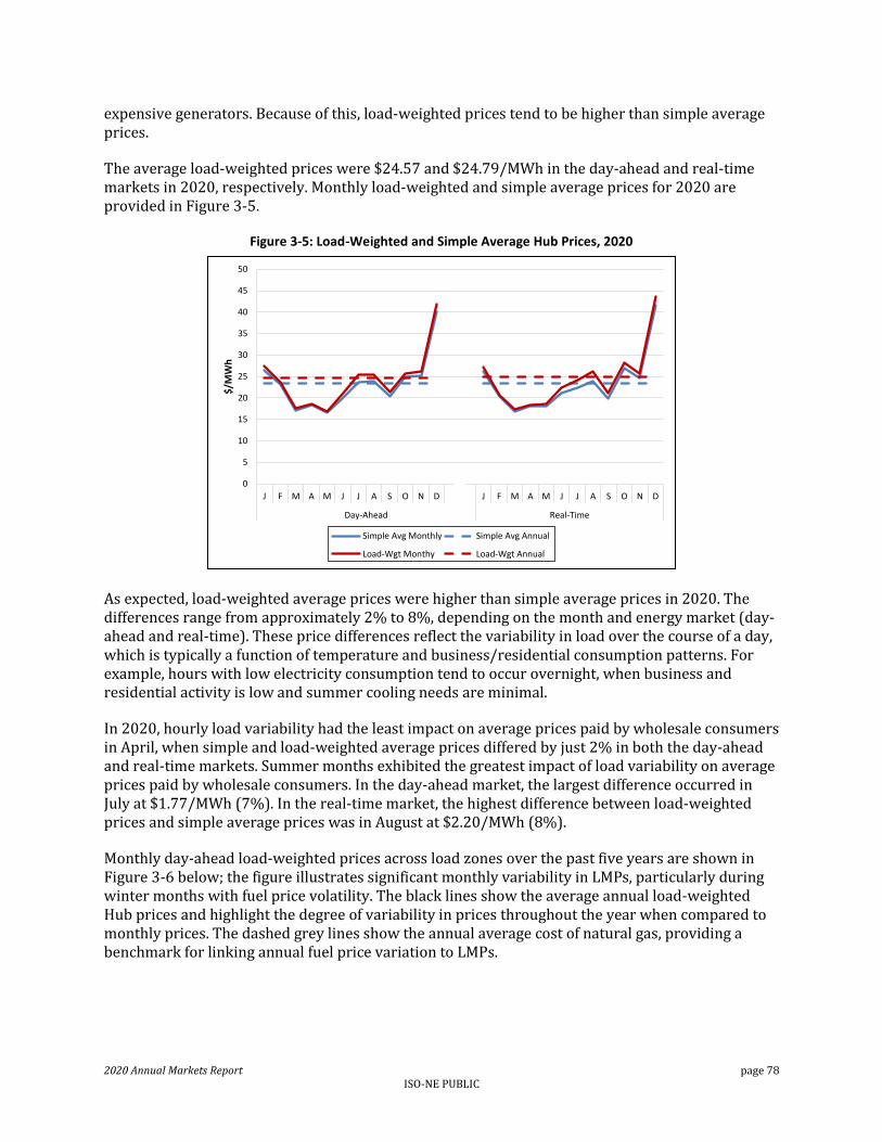
2020 Annual Markets Report page 78 ISO-NE PUBLIC
expensive generators. Because of this, load-weighted prices tend to be higher than simple average prices.
The average load-weighted prices were $24.57 and $24.79/MWh in the day-ahead and real-time markets in 2020, respectively. Monthly load-weighted and simple average prices for 2020 are provided in Figure 3-5.
Figure 3-5: Load-Weighted and Simple Average Hub Prices, 2020
As expected, load-weighted average prices were higher than simple average prices in 2020. The differences range from approximately 2% to 8%, depending on the month and energy market (day-ahead and real-time). These price differences reflect the variability in load over the course of a day, which is typically a function of temperature and business/residential consumption patterns. For example, hours with low electricity consumption tend to occur overnight, when business and residential activity is low and summer cooling needs are minimal.
In 2020, hourly load variability had the least impact on average prices paid by wholesale consumers in April, when simple and load-weighted average prices differed by just 2% in both the day-ahead and real-time markets. Summer months exhibited the greatest impact of load variability on average prices paid by wholesale consumers. In the day-ahead market, the largest difference occurred in July at $1.77/MWh (7%). In the real-time market, the highest difference between load-weighted prices and simple average prices was in August at $2.20/MWh (8%).
Monthly day-ahead load-weighted prices across load zones over the past five years are shown in Figure 3-6 below; the figure illustrates significant monthly variability in LMPs, particularly during winter months with fuel price volatility. The black lines show the average annual load-weighted Hub prices and highlight the degree of variability in prices throughout the year when compared to monthly prices. The dashed grey lines show the annual average cost of natural gas, providing a benchmark for linking annual fuel price variation to LMPs.
0
5
10
15
20
25
30
35
40
45
50
J F M A M J J A S O N D J F M A M J J A S O N D
Day-Ahead Real-Time
$/M
Wh
Simple Avg Monthly Simple Avg Annual
Load-Wgt Monthy Load-Wgt Annual
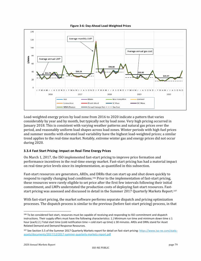
2020 Annual Markets Report page 79 ISO-NE PUBLIC
Figure 3-6: Day-Ahead Load-Weighted Prices
Load-weighted energy prices by load zone from 2016 to 2020 indicate a pattern that varies considerably by year and by month, but typically not by load zone. Very high pricing occurred in January 2018. This is consistent with varying weather patterns and natural gas prices over the period, and reasonably uniform load shapes across load zones. Winter periods with high fuel prices and summer months with elevated load variability have the highest load-weighted prices; a similar trend applies to the real-time market. Notably, extreme winter gas and energy prices did not occur during 2020.
3.3.4 Fast Start Pricing: Impact on Real-Time Energy Prices
On March 1, 2017, the ISO implemented fast-start pricing to improve price formation and performance incentives in the real-time energy market. Fast-start pricing has had a material impact on real-time price levels since its implementation, as quantified in this subsection.
Fast-start resources are generators, ARDs, and DRRs that can start up and shut down quickly to respond to rapidly changing load conditions.106 Prior to the implementation of fast-start pricing, these resources were rarely eligible to set price after the first few intervals following their initial commitment, and LMPs understated the production costs of deploying fast-start resources. Fast-start pricing was assessed and discussed in detail in the Summer 2017 Quarterly Markets Report.107
With fast-start pricing, the market software performs separate dispatch and pricing optimization processes. The dispatch process is similar to the previous (before fast-start pricing) process, in that
106 To be considered fast-start, resources must be capable of receiving and responding to ISO commitment and dispatch instructions. Their supply offers must have the following characteristics: 1.) Minimum run time and minimum down time ≤ 1 hour (each) 2.) Total start time (cold notification time + cold start-up time) ≤ 30 minutes. ARDs and DRRs stand for Asset Related Demand and Demand Response Resources.
107 See Section 5.5 of the Summer 2017 Quarterly Markets report for detail on fast-start pricing: https://www.iso-ne.com/static-assets/documents/2017/12/2017-summer-quarterly-markets-report.pdf
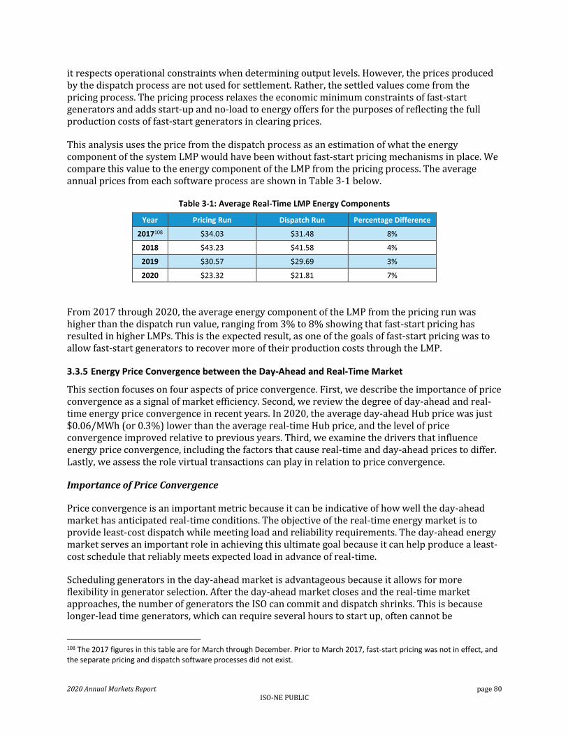
2020 Annual Markets Report page 80 ISO-NE PUBLIC
it respects operational constraints when determining output levels. However, the prices produced by the dispatch process are not used for settlement. Rather, the settled values come from the pricing process. The pricing process relaxes the economic minimum constraints of fast-start generators and adds start-up and no-load to energy offers for the purposes of reflecting the full production costs of fast-start generators in clearing prices.
This analysis uses the price from the dispatch process as an estimation of what the energy component of the system LMP would have been without fast-start pricing mechanisms in place. We compare this value to the energy component of the LMP from the pricing process. The average annual prices from each software process are shown in Table 3-1 below.
Table 3-1: Average Real-Time LMP Energy Components
Year Pricing Run Dispatch Run Percentage Difference
2017108 $34.03 $31.48 8%
2018 $43.23 $41.58 4%
2019 $30.57 $29.69 3%
2020 $23.32 $21.81 7%
From 2017 through 2020, the average energy component of the LMP from the pricing run was higher than the dispatch run value, ranging from 3% to 8% showing that fast-start pricing has resulted in higher LMPs. This is the expected result, as one of the goals of fast-start pricing was to allow fast-start generators to recover more of their production costs through the LMP.
3.3.5 Energy Price Convergence between the Day-Ahead and Real-Time Market
This section focuses on four aspects of price convergence. First, we describe the importance of price convergence as a signal of market efficiency. Second, we review the degree of day-ahead and real-time energy price convergence in recent years. In 2020, the average day-ahead Hub price was just $0.06/MWh (or 0.3%) lower than the average real-time Hub price, and the level of price convergence improved relative to previous years. Third, we examine the drivers that influence energy price convergence, including the factors that cause real-time and day-ahead prices to differ. Lastly, we assess the role virtual transactions can play in relation to price convergence.
Importance of Price Convergence
Price convergence is an important metric because it can be indicative of how well the day-ahead market has anticipated real-time conditions. The objective of the real-time energy market is to provide least-cost dispatch while meeting load and reliability requirements. The day-ahead energy market serves an important role in achieving this ultimate goal because it can help produce a least-cost schedule that reliably meets expected load in advance of real-time.
Scheduling generators in the day-ahead market is advantageous because it allows for more flexibility in generator selection. After the day-ahead market closes and the real-time market approaches, the number of generators the ISO can commit and dispatch shrinks. This is because longer-lead time generators, which can require several hours to start up, often cannot be
108 The 2017 figures in this table are for March through December. Prior to March 2017, fast-start pricing was not in effect, and the separate pricing and dispatch software processes did not exist.
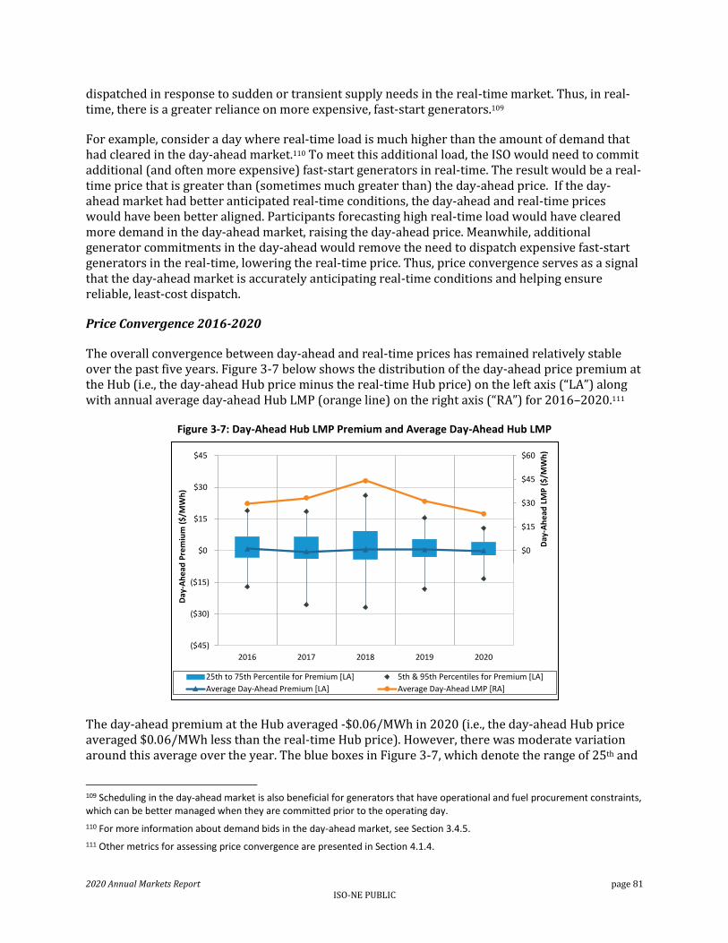
2020 Annual Markets Report page 81 ISO-NE PUBLIC
dispatched in response to sudden or transient supply needs in the real-time market. Thus, in real-time, there is a greater reliance on more expensive, fast-start generators.109
For example, consider a day where real-time load is much higher than the amount of demand that had cleared in the day-ahead market.110 To meet this additional load, the ISO would need to commit additional (and often more expensive) fast-start generators in real-time. The result would be a real-time price that is greater than (sometimes much greater than) the day-ahead price. If the day-ahead market had better anticipated real-time conditions, the day-ahead and real-time prices would have been better aligned. Participants forecasting high real-time load would have cleared more demand in the day-ahead market, raising the day-ahead price. Meanwhile, additional generator commitments in the day-ahead would remove the need to dispatch expensive fast-start generators in the real-time, lowering the real-time price. Thus, price convergence serves as a signal that the day-ahead market is accurately anticipating real-time conditions and helping ensure reliable, least-cost dispatch.
Price Convergence 2016-2020
The overall convergence between day-ahead and real-time prices has remained relatively stable over the past five years. Figure 3-7 below shows the distribution of the day-ahead price premium at the Hub (i.e., the day-ahead Hub price minus the real-time Hub price) on the left axis (“LA”) along with annual average day-ahead Hub LMP (orange line) on the right axis (“RA”) for 2016–2020.111
Figure 3-7: Day-Ahead Hub LMP Premium and Average Day-Ahead Hub LMP
The day-ahead premium at the Hub averaged -$0.06/MWh in 2020 (i.e., the day-ahead Hub price averaged $0.06/MWh less than the real-time Hub price). However, there was moderate variation around this average over the year. The blue boxes in Figure 3-7, which denote the range of 25th and
109 Scheduling in the day-ahead market is also beneficial for generators that have operational and fuel procurement constraints, which can be better managed when they are committed prior to the operating day.
110 For more information about demand bids in the day-ahead market, see Section 3.4.5.
111 Other metrics for assessing price convergence are presented in Section 4.1.4.
($60)
($45)
($30)
($15)
$0
$15
$30
$45
$60
($45)
($30)
($15)
$0
$15
$30
$45
2016 2017 2018 2019 2020
Day
-Ah
ead
LM
P (
$/M
Wh
)
Day
-Ah
ead
Pre
miu
m (
$/M
Wh
)
25th to 75th Percentile for Premium [LA] 5th & 95th Percentiles for Premium [LA]
Average Day-Ahead Premium [LA] Average Day-Ahead LMP [RA]

2020 Annual Markets Report page 82 ISO-NE PUBLIC
75th percentiles of the day-ahead premium for each year, show that for half of all hours in 2020, the day-ahead Hub premium was between -$2.15/MWh and $3.95/MWh. This is a narrower range than the previous four years. The whiskers in the figure show the 5th and 95th percentiles for the day-ahead Hub premium, which were -$13.31/MWh and $10.69/MWh, respectively, in 2020. The range between the 5th and 95th percentiles in 2020 ($24/MWh) was the lowest of the five-year reporting period. These narrowing ranges indicate improving price convergence, but it is important to note that, over time, these percentiles generally track the average day-ahead LMP (orange series, right axis). Since average LMPs are primarily driven by natural gas prices in New England, average LMPs tend to be higher when natural gas prices in New England are higher. Similarly, differences between day-ahead and real-time prices tend to be larger when gas prices are higher. This is because the difference in cost between two gas-fired generators with different heat rates is greater when gas prices are higher.112
Drivers of Price Divergence
Despite efforts to predict and anticipate real-time conditions in the day-ahead market, real-time conditions usually differ from day-ahead expectations. Market efficiency does not require that real-time and day-ahead prices be equal all the time. Rather, it means that prices reflect all available information, and in turn, day-ahead prices represent an unbiased expectation of real-time prices.
Ultimately, day-ahead and real-time prices are determined by energy supply, energy demand, and reliability actions taken by the ISO. Thus, when day-ahead and real-time prices do vary, the differences are often driven by shifts in supply and demand conditions. For example, if a generator clears an energy supply offer in the day-ahead market but experiences an unplanned outage in real-time, the available system supply falls and real-time prices will likely rise. On the demand-side, higher-than expected temperatures on a summer day can translate to greater real-time loads and higher real-time prices.
The close connection between deviations in real-time load and day-ahead demand and the differences in real-time and day-ahead Hub prices is shown in Figure 3-8 below. The green line depicts the average difference between day-ahead native demand and real-time metered native load (i.e., day-ahead demand minus real-time load) during 2020 by hour of the day (hours ending 1–24).113 The blue line shows the median difference between day-ahead and real-time Hub prices (i.e., day-ahead Hub price minus real-time Hub price) during 2020 by hour of the day.
112 For example, consider two gas-fired generators: Gen A has a heat rate of 7 MMBtu/MWh and Gen B has a heat rate of 10 MMBtu/MWh. If the gas price is $5/MMBtu, the generation cost for Gen A is $35/MWh (7 MMBtu/MWh x $5/MMBtu) and the cost for Gen B is $50/MWh (10 MMBtu/MWh x $5/MMBtu). The difference in generation cost between Gen A and Gen B is $15/MWh. If the gas price increases to $10/MMBtu, the generation costs for Gen A and Gen B are now $70/MWh and $100/MWh, respectively, for a difference of $30/MWh.
113 The term Demand is used to refer to the day-ahead market cleared quantity and Load is used to refer to the real-time market cleared quantity due to the distinction between the markets in that the day-ahead is a financial market that allows both physical and virtual transactions while the real-time is physical only market.
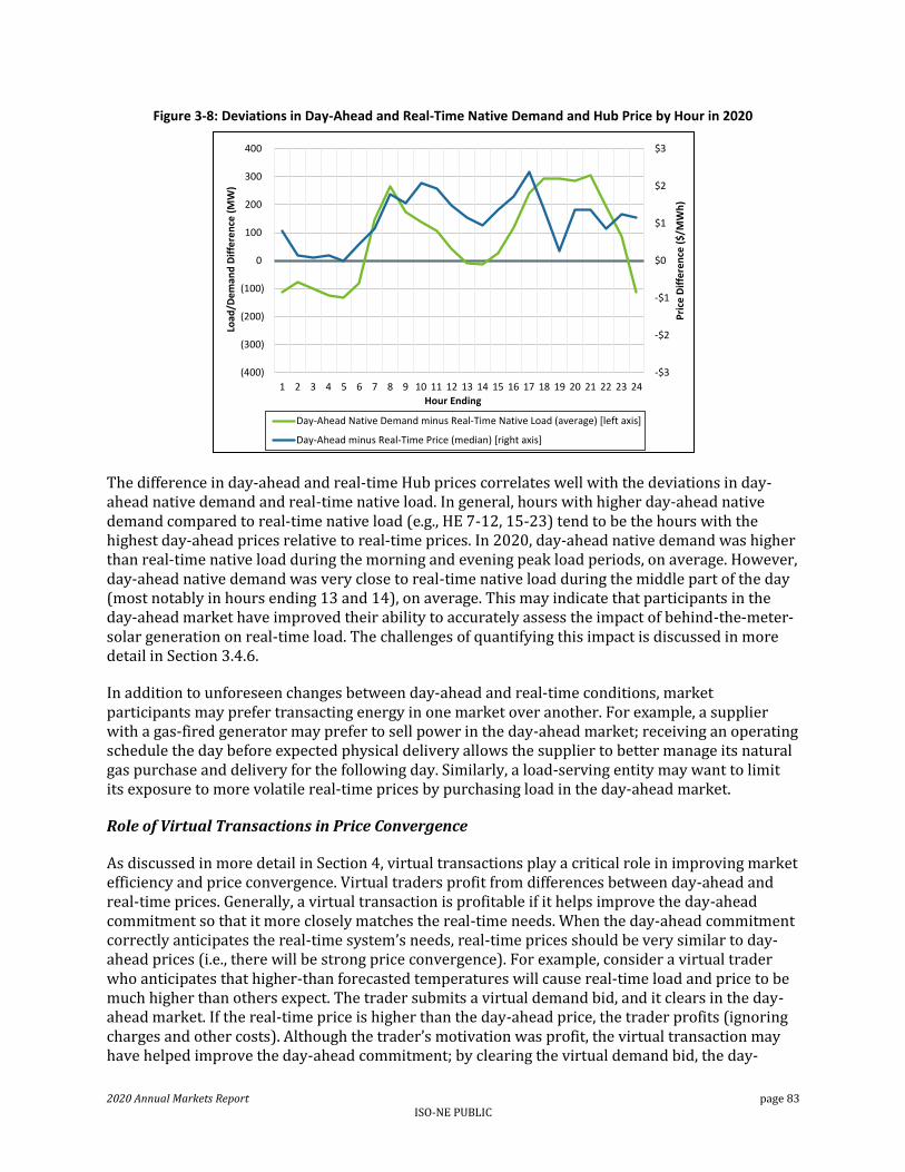
2020 Annual Markets Report page 83 ISO-NE PUBLIC
Figure 3-8: Deviations in Day-Ahead and Real-Time Native Demand and Hub Price by Hour in 2020
The difference in day-ahead and real-time Hub prices correlates well with the deviations in day-ahead native demand and real-time native load. In general, hours with higher day-ahead native demand compared to real-time native load (e.g., HE 7-12, 15-23) tend to be the hours with the highest day-ahead prices relative to real-time prices. In 2020, day-ahead native demand was higher than real-time native load during the morning and evening peak load periods, on average. However, day-ahead native demand was very close to real-time native load during the middle part of the day (most notably in hours ending 13 and 14), on average. This may indicate that participants in the day-ahead market have improved their ability to accurately assess the impact of behind-the-meter-solar generation on real-time load. The challenges of quantifying this impact is discussed in more detail in Section 3.4.6.
In addition to unforeseen changes between day-ahead and real-time conditions, market participants may prefer transacting energy in one market over another. For example, a supplier with a gas-fired generator may prefer to sell power in the day-ahead market; receiving an operating schedule the day before expected physical delivery allows the supplier to better manage its natural gas purchase and delivery for the following day. Similarly, a load-serving entity may want to limit its exposure to more volatile real-time prices by purchasing load in the day-ahead market.
Role of Virtual Transactions in Price Convergence
As discussed in more detail in Section 4, virtual transactions play a critical role in improving market efficiency and price convergence. Virtual traders profit from differences between day-ahead and real-time prices. Generally, a virtual transaction is profitable if it helps improve the day-ahead commitment so that it more closely matches the real-time needs. When the day-ahead commitment correctly anticipates the real-time system’s needs, real-time prices should be very similar to day-ahead prices (i.e., there will be strong price convergence). For example, consider a virtual trader who anticipates that higher-than forecasted temperatures will cause real-time load and price to be much higher than others expect. The trader submits a virtual demand bid, and it clears in the day-ahead market. If the real-time price is higher than the day-ahead price, the trader profits (ignoring charges and other costs). Although the trader’s motivation was profit, the virtual transaction may have helped improve the day-ahead commitment; by clearing the virtual demand bid, the day-
-$3
-$2
-$1
$0
$1
$2
$3
(400)
(300)
(200)
(100)
0
100
200
300
400
1 2 3 4 5 6 7 8 9 10 11 12 13 14 15 16 17 18 19 20 21 22 23 24
Pri
ce D
iffe
ren
ce (
$/M
Wh
)
Load
/De
man
d D
iffe
ren
ce (
MW
)
Hour Ending
Day-Ahead Native Demand minus Real-Time Native Load (average) [left axis]
Day-Ahead minus Real-Time Price (median) [right axis]
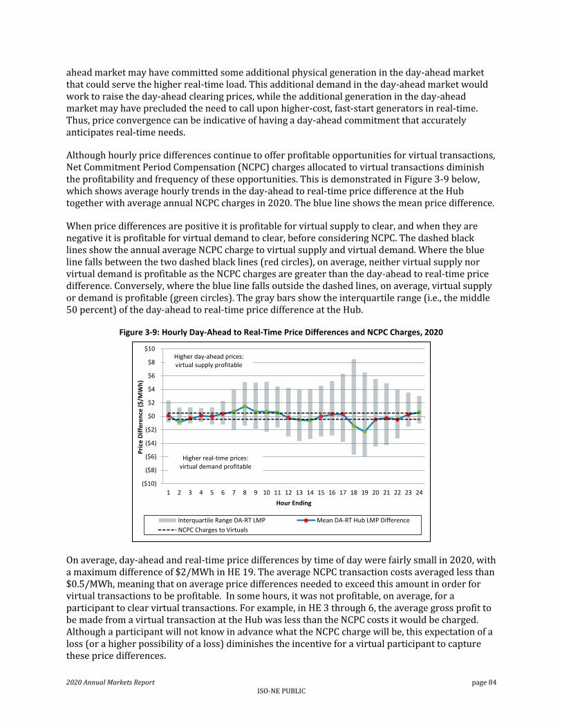
2020 Annual Markets Report page 84 ISO-NE PUBLIC
ahead market may have committed some additional physical generation in the day-ahead market that could serve the higher real-time load. This additional demand in the day-ahead market would work to raise the day-ahead clearing prices, while the additional generation in the day-ahead market may have precluded the need to call upon higher-cost, fast-start generators in real-time. Thus, price convergence can be indicative of having a day-ahead commitment that accurately anticipates real-time needs.
Although hourly price differences continue to offer profitable opportunities for virtual transactions, Net Commitment Period Compensation (NCPC) charges allocated to virtual transactions diminish the profitability and frequency of these opportunities. This is demonstrated in Figure 3-9 below, which shows average hourly trends in the day-ahead to real-time price difference at the Hub together with average annual NCPC charges in 2020. The blue line shows the mean price difference.
When price differences are positive it is profitable for virtual supply to clear, and when they are negative it is profitable for virtual demand to clear, before considering NCPC. The dashed black lines show the annual average NCPC charge to virtual supply and virtual demand. Where the blue line falls between the two dashed black lines (red circles), on average, neither virtual supply nor virtual demand is profitable as the NCPC charges are greater than the day-ahead to real-time price difference. Conversely, where the blue line falls outside the dashed lines, on average, virtual supply or demand is profitable (green circles). The gray bars show the interquartile range (i.e., the middle 50 percent) of the day-ahead to real-time price difference at the Hub.
Figure 3-9: Hourly Day-Ahead to Real-Time Price Differences and NCPC Charges, 2020
On average, day-ahead and real-time price differences by time of day were fairly small in 2020, with a maximum difference of $2/MWh in HE 19. The average NCPC transaction costs averaged less than $0.5/MWh, meaning that on average price differences needed to exceed this amount in order for virtual transactions to be profitable. In some hours, it was not profitable, on average, for a participant to clear virtual transactions. For example, in HE 3 through 6, the average gross profit to be made from a virtual transaction at the Hub was less than the NCPC costs it would be charged. Although a participant will not know in advance what the NCPC charge will be, this expectation of a loss (or a higher possibility of a loss) diminishes the incentive for a virtual participant to capture these price differences.
($10)
($8)
($6)
($4)
($2)
$0
$2
$4
$6
$8
$10
1 2 3 4 5 6 7 8 9 10 11 12 13 14 15 16 17 18 19 20 21 22 23 24
Pri
ce D
iffe
ren
ce (
$/M
Wh
)
Hour Ending
Interquartile Range DA-RT LMP Mean DA-RT Hub LMP Difference
NCPC Charges to Virtuals
Higher day-ahead prices: virtual supply profitable
Higher real-time prices: virtual demand profitable

2020 Annual Markets Report page 85 ISO-NE PUBLIC
However in other hours, it was profitable, on average, for virtual traders to clear virtual transactions, yet this did not occur. One period where this is most apparent for hours ending 8 through 11, when day-ahead prices were, on average, above real-time prices and this difference exceeded the average NCPC charge. It would have been profitable, on average, for a participant to clear virtual supply in the day-ahead market in these hours — effectively selling at the higher day-ahead price and buying back at the lower real-time price. Arbitraging this price difference may be hindered to some degree by uncertainty over NCPC charges or uncertain load conditions in these hours, with the latter being increasingly impacted by the growth in behind-the-meter solar generation.
3.4 Drivers of Energy Market Outcomes
Many factors can provide important insights into long-term market trends. For example, underlying natural gas prices can explain, to a large degree, movements in energy prices. Other factors, such as load forecast error or notable system events can provide additional insight into specific short-term pricing outcomes. This section covers some of the important factors that provide context to energy market outcomes. The section is structured as follows:
Generation costs (Section 3.4.1) Supply-side participation (Section 3.4.2) Reserve Adequacy Analysis (RAA) Commitments (Section 3.4.3) Load and weather conditions (Section 3.4.4) Demand bidding (Section 3.4.5) Load forecast error (Section 3.4.6) Reserve margin (Section3.4.7) System events (Section 3.4.8) Reliability commitments (Section 3.4.9) Congestion (Section 3.4.10) Marginal resources (Section 3.4.11)
3.4.1 Generation Costs
Day-ahead and real-time electricity prices in New England continue to be closely correlated with the estimated cost of operating a natural gas-fired generator. As discussed later in Section 3.4.11, one or more marginal resources determine the price of electricity in any given time interval. In a competitive, uniform clearing price auction, a resource’s offer price should reflect its variable production costs. For fossil fuel-fired generators, their variable costs are largely determined by their fuel costs and operating efficiencies (heat rates). Since natural gas-fired generators set price more frequently than generators of any other fuel type in New England, electricity prices are positively correlated with the estimated marginal cost of a typical natural gas-fired generator.
One way to understand the relationship between electricity prices and fuel costs is to compare the variable costs of different fuel types to the wholesale price (LMP). Quarterly average on-peak, day-ahead LMPs and estimated generation costs of various fuel types (assuming standard heat rates),

2020 Annual Markets Report page 86 ISO-NE PUBLIC
and spark spreads (or the estimated profitability of a natural gas-fired generator) are shown below in Figure 3-10.114
Figure 3-10: Estimated Generation Costs and On-Peak LMPs
Figure 3-10 shows that prices are closely correlated with the estimated costs of operating a natural gas-fired generator. The correlation varies within each year, especially during the summer when electricity demand is typically higher. Higher demand typically requires the operation of less efficient natural gas-fired generators and/or generators that burn more expensive fuels. During the summer months, efficient natural gas-fired generators earn higher margins (commonly referred to as spark spreads) compared to other months.115
In New England, natural gas-fired generators are the dominant price setters and supply over 50% of native generation. Therefore, it is worth reviewing trends in industry-standard profitability metrics for gas-fired generators. Such metrics include implied heat rates and spark spreads across a range of efficiencies applicable to the New England fleet of natural gas-fired generators.
Table 3-2 shows the average day-ahead on-peak LMP and the annual average natural gas price; these are the key inputs into the calculation of the implied heat rate (or breakeven point) for
114 Variable generation costs are calculated by multiplying the average daily fuel price ($/MMBtu) by the average standard efficiency of generators of a given technology and fuel type. Our standard heat rates are measured in MMBtu/MWh as follows: Natural Gas 7.8, Coal – 10.0, No. 6 Oil – 10.7, No. 2 Oil – 11.7. The spark spread is the difference between the LMP and the fuel cost of a gas-fired generator with a heat rate of 7.8.
115 During the winter months, coal- and oil-fired generators, as well as imports, can displace natural gas-fired generators in economic merit order more frequently than in other seasons, as natural gas prices increase due to gas network demand and constraints. This tends to lessen the impact of higher gas prices on LMPs as more costly gas-fired generators are pushed out of merit and leads to reduced spark spreads.
$0
$20
$40
$60
$80
$100
$120
$140
$160
$180
$200
Q1 Q2 Q3 Q4 Q1 Q2 Q3 Q4 Q1 Q2 Q3 Q4 Q1 Q2 Q3 Q4 Q1 Q2 Q3 Q4
2016 2017 2018 2019 2020
$/M
Wh
Quarterly Values
Spark Spread DA LMP Natural Gas Coal No.6 Oil No.2 Oil Diesel
$0
$10
$20
$30
$40
$50
$60
2016 2017 2018 2019 2020
Annual Values (excl. oil)
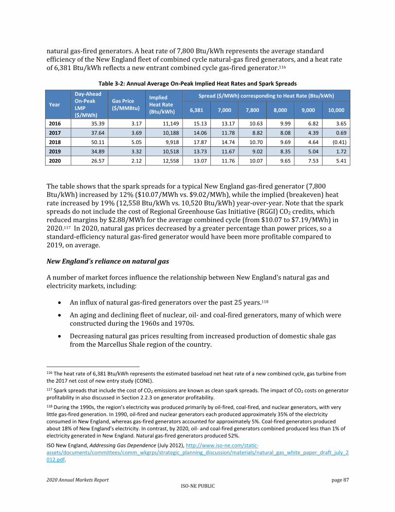
2020 Annual Markets Report page 87 ISO-NE PUBLIC
natural gas-fired generators. A heat rate of 7,800 Btu/kWh represents the average standard efficiency of the New England fleet of combined cycle natural-gas fired generators, and a heat rate of 6,381 Btu/kWh reflects a new entrant combined cycle gas-fired generator.116
Table 3-2: Annual Average On-Peak Implied Heat Rates and Spark Spreads
Year
Day-Ahead On-Peak LMP ($/MWh)
Gas Price ($/MMBtu)
Implied Heat Rate (Btu/kWh)
Spread ($/MWh) corresponding to Heat Rate (Btu/kWh)
6,381 7,000 7,800 8,000 9,000 10,000
2016 35.39 3.17 11,149 15.13 13.17 10.63 9.99 6.82 3.65
2017 37.64 3.69 10,188 14.06 11.78 8.82 8.08 4.39 0.69
2018 50.11 5.05 9,918 17.87 14.74 10.70 9.69 4.64 (0.41)
2019 34.89 3.32 10,518 13.73 11.67 9.02 8.35 5.04 1.72
2020 26.57 2.12 12,558 13.07 11.76 10.07 9.65 7.53 5.41
The table shows that the spark spreads for a typical New England gas-fired generator (7,800 Btu/kWh) increased by 12% ($10.07/MWh vs. $9.02/MWh), while the implied (breakeven) heat rate increased by 19% (12,558 Btu/kWh vs. 10,520 Btu/kWh) year-over-year. Note that the spark spreads do not include the cost of Regional Greenhouse Gas Initiative (RGGI) CO2 credits, which reduced margins by $2.88/MWh for the average combined cycle (from $10.07 to $7.19/MWh) in 2020.117 In 2020, natural gas prices decreased by a greater percentage than power prices, so a standard-efficiency natural gas-fired generator would have been more profitable compared to 2019, on average.
New England’s reliance on natural gas
A number of market forces influence the relationship between New England’s natural gas and electricity markets, including:
An influx of natural gas-fired generators over the past 25 years.118
An aging and declining fleet of nuclear, oil- and coal-fired generators, many of which were constructed during the 1960s and 1970s.
Decreasing natural gas prices resulting from increased production of domestic shale gas from the Marcellus Shale region of the country.
116 The heat rate of 6,381 Btu/kWh represents the estimated baseload net heat rate of a new combined cycle, gas turbine from the 2017 net cost of new entry study (CONE).
117 Spark spreads that include the cost of CO2 emissions are known as clean spark spreads. The impact of CO2 costs on generator profitability in also discussed in Section 2.2.3 on generator profitability.
118 During the 1990s, the region’s electricity was produced primarily by oil-fired, coal-fired, and nuclear generators, with very little gas-fired generation. In 1990, oil-fired and nuclear generators each produced approximately 35% of the electricity consumed in New England, whereas gas-fired generators accounted for approximately 5%. Coal-fired generators produced about 18% of New England’s electricity. In contrast, by 2020, oil- and coal-fired generators combined produced less than 1% of electricity generated in New England. Natural gas-fired generators produced 52%.
ISO New England, Addressing Gas Dependence (July 2012), http://www.iso-ne.com/static-assets/documents/committees/comm_wkgrps/strategic_planning_discussion/materials/natural_gas_white_paper_draft_july_2012.pdf.
2020 Annual Markets Report page 88 ISO-NE PUBLIC
Increasing constraints on the natural gas system due to high heating demand during winter months and greater demand from a larger fleet of natural gas-fired generators. Limited additional gas pipeline capacity has been developed to alleviate these constraints due to regulatory, political and market challenges.
The first three factors listed above have resulted in gas-fired generators supplying a much higher proportion of electricity in New England than ever before. However, during winter months, gas-fired generators must compete with heating demand, which can push gas pipeline capacity to its limit over periods with peak gas demand. Consequently, the reliability of New England’s wholesale electricity grid is partially dependent on the owners and operators of natural gas-fired generators effectively managing natural gas deliveries during contemporaneous periods of high gas and electric power demand. Reliability is also increasingly dependent on the region’s oil fleet having sufficient oil inventory to operate when the gas network is highly constrained. During these periods, oil-fired generation can be cheaper than gas-fired generation, leading to oil-fired generators being dispatched more frequently.
One of the challenges identified in the ISO’s Strategic Planning Initiative is the region’s reliance on natural gas-fired generators.119 Over the past few years the ISO has undertaken a number of related initiatives, including the following:
Redesigning Forward Capacity Market performance penalties with the pay-for-performance (PFP) capacity market design, which began June 1, 2018. 120
Introducing the Winter Reliability Program, which was in place until PFP was implemented in 2018.
Allowing the ISO to share information concerning the scheduled output of natural gas-fired generators with the operating personnel of the interstate natural gas pipeline companies serving New England.
Introducing changes to the energy market design, including improving price signals for fast-start resources, accelerating the closing time of the day-ahead energy market (May 2013) and introducing energy market offer flexibility in December 2014.
Increasing the procurement of ten-minute non-spinning reserves in the Forward Reserve Market to account for generator non-performance.
Including an Energy Market Opportunity Cost (EMOC) adder in energy market reference levels for generators that maintain an oil inventory. Beginning in December 2018, EMOC allows participants to reflect the value of limited fuel in the mitigation process so that it can be preserved for hours when it is most economic and needed to alleviate tight system conditions.
A one-year program, known as the Interim Compensation Treatment, to compensate generators for making fuel arrangements for Winter 2023/4.
119 See the ISO’s “Strategic Planning Initiative Key Project” webpage at http://www.iso-ne.com/committees/key-projects/implemented/strategic-planning-initiative.
120 See Section 6.2.2 for information on pay-for-performance

2020 Annual Markets Report page 89 ISO-NE PUBLIC
Relationship between natural gas and electricity prices
Average annual day-ahead on-peak LMPs (left axis, “LA”) and natural gas prices (right axis, “RA”) from 2016 to 2020 are shown in Figure 3-11 below. Since cold weather in the first quarter (Q1) can cause higher natural gas prices and electricity prices, Q1 is shown separately from the rest of the year.
Figure 3-11: Average Electricity and Gas Prices for Q1 Compared with Rest of Year
Colder temperatures in Q1 tend to cause higher natural gas prices and LMPs than in the rest of the year. In Q1 2020, gas prices averaged $2.33/MMBtu compared to $2.02/MMBtu during the rest of the year. However, mild weather and lower loads during the winter (Q1) led to lower LMPs during Q1 2020 than during the rest of the year (Q2 - Q4). LMPs in Q1 2020 were slightly lower, averaging $23.86/MWh compared to $26.11/MWh during the rest of the year. LMPs were lower during the winter despite higher gas prices. This was due to higher average load during the rest of the year (combined) requiring higher-cost generation (and resulting in higher spark spreads), as well as higher emissions costs.
Compared to prior winters, warmer temperatures in Q1 2020 resulted in lower natural gas prices and day-ahead on-peak LMPs than any other Q1 over the reporting period. In Q1 2020, natural gas prices ($2.33/MMBtu) were between 30% and 72% lower and LMPs were between 27% and 64% lower than the previous four winters, on average. In Q1 2020, temperatures averaged 36⁰F, a 5⁰F increase compared to the Q1 2019 average temperature and 3⁰F warmer than the five-year average temperature (33⁰F).
Lower gas prices and milder weather also resulted in lower LNG injections into the New England interstate gas system. When the primary natural gas pipelines (which flow from west and south) become constrained, LNG deliveries can provide counter flow (or injections from the east and north). This helps alleviate natural gas constraints and puts downward pressure on natural gas prices. LNG injections into New England during Q1 2020 decreased by 26% compared to Q1 2019, falling from 21.9 million Dth to 16.2 million Dth. The year-over-year decrease in LNG was equivalent to the amount of natural gas necessary to run a 340 MW standard heat rate natural gas-fired generator for the entire quarter.

2020 Annual Markets Report page 90 ISO-NE PUBLIC
Natural Gas Price-Adjusted LMP
As discussed, changes in LMPs are generally strongly positively correlated with changes in natural gas prices in New England. Changes in LMPs are also influenced by a number of other factors, including supply mix changes, system demand levels, and unanticipated events such as forced equipment outages. The gas price-adjusted LMP is a high level metric used to estimate the impact of these of non-gas price factors on the energy price.
The gas price-adjusted LMP is derived by dividing the reference year natural gas price (2016) by the current year natural gas price, then multiplying by the load-weighted LMP. The day-ahead (blue solid) and real-time (red solid) gas-price adjusted LMPs and the day-ahead (blue dashed) and real-time (red dashed) load-weighted LMPs from 2016 to 2020 are shown in the Figure 3-12 below.
Figure 3-12: Annual Average Natural Gas Price-Adjusted LMPs
After adjusting for gas prices, the day-ahead and real-time LMPs were within a relatively narrow band from 2016 (the reference year) to 2019, indicating gas prices had a relatively large impact on the LMP. Over the period shown, the gas price-adjusted LMP reached its highest price in 2020, as the average load-weighted day-ahead and real-time LMPs decreased (by 24-25%) by less than the change in the gas price (down by 36%). On a gas price-adjusted basis, day-ahead and real-time prices increased by 16% (from $31.38 to $36.52/MWh) and 19% (from $30.90 to $36.84/MWh), respectively, on average. As discussed in Section 2.1, this is largely due to two non-gas factors: lower fixed supply with a reduction in nuclear generation in 2020, and to a lesser extent, an increase in CO2 emissions costs under the Regional Greenhouse Gas Initiative (RGGI) program.
Energy Market Opportunity Cost
Winter 2020/21 produced the first non-zero energy market opportunity costs (EMOCs) since their implementation.121 On December 1, 2018, energy market reference levels began including an
121 In this section, winter is defined as December through February, which is different from the calendar winter period of January through March used in other parts of this report.
$0
$10
$20
$30
$40
$50
$60
2016 2017 2018 2019 2020
$/M
Wh
DA Gas-Adjusted LMP RT Gas-Adjusted LMP
RT LMP (Load-Weighted) DA LMP (Load-Weighted)
Reference Year: 2016

2020 Annual Markets Report page 91 ISO-NE PUBLIC
opportunity cost adder for generators that maintain an oil inventory.122 The update was motivated by concerns that, during sustained cold weather events, generators were unable to make energy supply offers that incorporated opportunity costs associated with the depletion of their limited fuel stock. Such an event arose during Winter 2017/18, which resulted in ISO operators posturing oil-fired generators to conserve oil inventories. During cold weather events, the inclusion of opportunity costs in energy offers enables the market to preserve limited fuel for hours when it is most economic and needed to alleviate tight system conditions.
Generator-specific EMOC adders are calculated with a mixed-integer programming model that was developed by the ISO and runs automatically each morning. For a given forecast of LMPs and fuel prices, the model seeks to maximize a generator’s net revenue by optimizing fuel use over a seven-day horizon, subject to constraints on fuel inventory and asset operational characteristics. Opportunity costs produced by the model are available to participants an hour before the day-ahead market closes and, since December 2019, a real-time opportunity cost update is available at 6:30 pm, on the day prior to real-time operation.123
While the calculation of EMOCs is complex and dependent on a number of variables, (e.g., gas and oil price forecasts, fuel inventory levels, and generator characteristics) it is possible to develop a general sense about when EMOCs are likely to occur. Primarily, we should expect to see EMOCs for a generator when oil prices are forecasted to be close to gas prices for a long enough period to physically exhaust the oil-fired generator’s inventory. This type of scenario would typically occur during an extended period of very cold weather when demand for natural gas is highest because natural gas is used for both heating and electricity generation in New England.
Winter 2020/21 did not have a cold snap as extreme as Winter 2017/18, but there was a sustained drop in average temperatures that was sufficient to produce non-zero EMOCs for two small generators. This was the first time a non-zero EMOC was incorporated into a generator’s offer since the inception of the program in in 2018.
One small generator (5 MW) had non-zero EMOCs for seven days from February 6 through February 12.
A second small generator (2MW) had a non-zero EMOC on February 8. The average daily temperature was just below 24⁰F for the seven days. The average EMOC was $7.54 per MWh across the seven days; this is added to the cost-
based reference level.
The short cold snap in Winter 2020/21 can be seen when comparing New England average daily temperatures with those from Winter 2019/20 as shown in Figure 3-13 below. Winter 2019/20 was generally milder than this past winter and did not have any extended very cold spells. By contrast, Winter 2020/21 had one short-lived cold snap (highlighted by the green circle) which narrowed the spread between oil and gas prices close to parity.
122 See https://www.iso-ne.com/static-assets/documents/2018/10/a7_memo_re_energy_market_opp_costs_for_oil_and_dual_fuel_revised_edition.pdf
123 The real-time update of the opportunity cost calculation is based on data that is available after the day-ahead market closes but prior to the start of the real-time market. This calculation incorporates updated fuel price forecasts to produce more accurate opportunity costs for the real-time market.
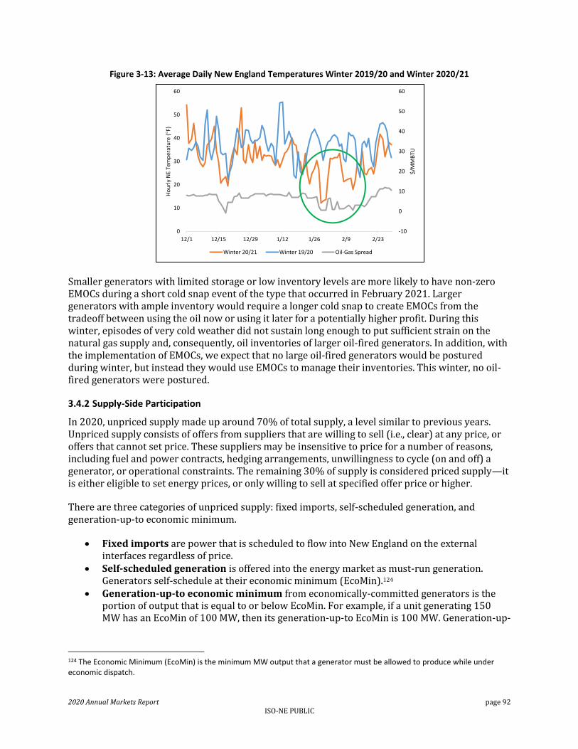
2020 Annual Markets Report page 92 ISO-NE PUBLIC
Figure 3-13: Average Daily New England Temperatures Winter 2019/20 and Winter 2020/21
Smaller generators with limited storage or low inventory levels are more likely to have non-zero EMOCs during a short cold snap event of the type that occurred in February 2021. Larger generators with ample inventory would require a longer cold snap to create EMOCs from the tradeoff between using the oil now or using it later for a potentially higher profit. During this winter, episodes of very cold weather did not sustain long enough to put sufficient strain on the natural gas supply and, consequently, oil inventories of larger oil-fired generators. In addition, with the implementation of EMOCs, we expect that no large oil-fired generators would be postured during winter, but instead they would use EMOCs to manage their inventories. This winter, no oil-fired generators were postured.
3.4.2 Supply-Side Participation
In 2020, unpriced supply made up around 70% of total supply, a level similar to previous years. Unpriced supply consists of offers from suppliers that are willing to sell (i.e., clear) at any price, or offers that cannot set price. These suppliers may be insensitive to price for a number of reasons, including fuel and power contracts, hedging arrangements, unwillingness to cycle (on and off) a generator, or operational constraints. The remaining 30% of supply is considered priced supply—it is either eligible to set energy prices, or only willing to sell at specified offer price or higher.
There are three categories of unpriced supply: fixed imports, self-scheduled generation, and generation-up-to economic minimum.
Fixed imports are power that is scheduled to flow into New England on the external interfaces regardless of price.
Self-scheduled generation is offered into the energy market as must-run generation. Generators self-schedule at their economic minimum (EcoMin).124
Generation-up-to economic minimum from economically-committed generators is the portion of output that is equal to or below EcoMin. For example, if a unit generating 150 MW has an EcoMin of 100 MW, then its generation-up-to EcoMin is 100 MW. Generation-up-
124 The Economic Minimum (EcoMin) is the minimum MW output that a generator must be allowed to produce while under economic dispatch.
-10
0
10
20
30
40
50
60
0
10
20
30
40
50
60
12/1 12/15 12/29 1/12 1/26 2/9 2/23
$/M
MB
TU
Ho
url
y N
E Te
mp
erat
ure
( F
)
Winter 20/21 Winter 19/20 Oil-Gas Spread
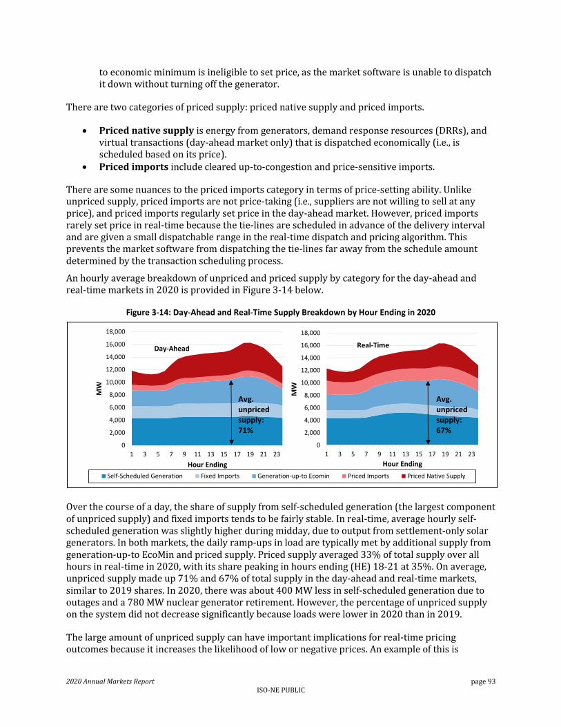
2020 Annual Markets Report page 93 ISO-NE PUBLIC
to economic minimum is ineligible to set price, as the market software is unable to dispatch it down without turning off the generator.
There are two categories of priced supply: priced native supply and priced imports.
Priced native supply is energy from generators, demand response resources (DRRs), and virtual transactions (day-ahead market only) that is dispatched economically (i.e., is scheduled based on its price).
Priced imports include cleared up-to-congestion and price-sensitive imports.
There are some nuances to the priced imports category in terms of price-setting ability. Unlike unpriced supply, priced imports are not price-taking (i.e., suppliers are not willing to sell at any price), and priced imports regularly set price in the day-ahead market. However, priced imports rarely set price in real-time because the tie-lines are scheduled in advance of the delivery interval and are given a small dispatchable range in the real-time dispatch and pricing algorithm. This prevents the market software from dispatching the tie-lines far away from the schedule amount determined by the transaction scheduling process.
An hourly average breakdown of unpriced and priced supply by category for the day-ahead and real-time markets in 2020 is provided in Figure 3-14 below.
Figure 3-14: Day-Ahead and Real-Time Supply Breakdown by Hour Ending in 2020
Over the course of a day, the share of supply from self-scheduled generation (the largest component of unpriced supply) and fixed imports tends to be fairly stable. In real-time, average hourly self-scheduled generation was slightly higher during midday, due to output from settlement-only solar generators. In both markets, the daily ramp-ups in load are typically met by additional supply from generation-up-to EcoMin and priced supply. Priced supply averaged 33% of total supply over all hours in real-time in 2020, with its share peaking in hours ending (HE) 18-21 at 35%. On average, unpriced supply made up 71% and 67% of total supply in the day-ahead and real-time markets, similar to 2019 shares. In 2020, there was about 400 MW less in self-scheduled generation due to outages and a 780 MW nuclear generator retirement. However, the percentage of unpriced supply on the system did not decrease significantly because loads were lower in 2020 than in 2019.
The large amount of unpriced supply can have important implications for real-time pricing outcomes because it increases the likelihood of low or negative prices. An example of this is
0
2,000
4,000
6,000
8,000
10,000
12,000
14,000
16,000
18,000
1 3 5 7 9 11 13 15 17 19 21 23
MW
Hour Ending
Day-Ahead
Self-Scheduled Generation Fixed Imports Generation-up-to Ecomin Priced Imports Priced Native Supply
0
2,000
4,000
6,000
8,000
10,000
12,000
14,000
16,000
18,000
1 3 5 7 9 11 13 15 17 19 21 23
MW
Hour Ending
Real-Time
Avg. unpriced supply: 71%
Avg. unpriced supply: 67%

2020 Annual Markets Report page 94 ISO-NE PUBLIC
illustrated in Figure 3-15 below, which shows unpriced and priced supply along with the Hub LMP for February 25-26, 2020. Unlike the figure above, this figure includes all imports in the fixed supply category for convenient illustrative purposes.
Figure 3-15: Price and Unpriced Supply vs. Real-Time LMP, February 25-26, 2020
In the early morning hours of February 26, real-time loads were relatively low, and as a result, the ISO only had to dispatch a small amount of priced generation. The small amount of generation dispatched economically had offered into the market with negative offers, resulting in negative prices. The 5-minute Hub LMP fell to about -$25/MWh from 01:00 to 01:15, and the hourly price averaged -$5.73/MWh during HE 2.
In situations like this, there is very little generation with price-setting capability on the system. The combination of low loads with large amounts of unpriced generation can thus bring about a sudden drop in prices, to low or even negative levels. However, the overall frequency of negative real-time prices at the Hub remains relatively low. Negative prices at the Hub occurred in 0.6% and 0.3% of hours in 2019 and 2020, respectively. Even in Maine, which tends to have a higher frequency of negative nodal prices at export-constrained pockets with wind generation, the hourly zonal price was negative in only 0.4% of hours in 2020.
3.4.3 Reserve Adequacy Analysis Commitments
The day-ahead market is a forward financial market that clears at the intersection of participant submitted supply offers and demand bids. However, the commitment, dispatch and pricing outcomes in the day-ahead market may not always reflect expected real-time conditions. For example, load-serving entities may clear less demand than the ISO’s load forecast. ISO-NE must ensure there is enough capacity and reserves to meet forecasted real-time load and reserve requirements. After the day-ahead market and the re-offer period close, the ISO performs the Reserve Adequacy Analysis (RAA) to meet these capacity and reserve constraints. If the day-ahead market satisfies the expected real-time requirement, additional generators will not need to be committed in the RAA process. Conversely, if the day-ahead market did not clear enough supply to meet the ISO’s forecasted demand and reserve, additional generators may be required.
-10
-5
0
5
10
15
20
25
30
0
2,000
4,000
6,000
8,000
10,000
12,000
14,000
16,000
18,000
1 3 5 7 9 11 13 15 17 19 21 23 1 3 5 7 9 11 13 15 17 19 21 23
2/25/2020 2/26/2020
$/M
Wh
MW
Fixed Supply Priced Supply Real-Time Hub LMP (hourly)
This led to low LMPs.
Low loads overnight resulted in relatively little priced supply on the system, and generators with low offers set price.

2020 Annual Markets Report page 95 ISO-NE PUBLIC
The difference between amount of physical cleared generation in the day-ahead market compared to the expected load and reserve requirement (the energy gap) and the commitments made in the RAA are shown in Figure 3-16 below. Large energy gaps are more likely to result in more RAA commitments. By comparing the energy gap to the additional non-fast start and non-LSCPR commitments made in the RAA, we can derive insights into different outcomes between each market.
Figure 3-16: RAA Generator Commitments and the Day-Ahead Energy Gap
RAA commitments remained very low in 2020, with the RAA process committing less than 10 MW per hour on average. The day-ahead market generally cleared sufficient supply and online generation capacity to meet the ISO’s load forecast and reserve requirements. In the day-ahead market, load-serving entities cleared more demand than what they consumed in the real-time market.125 Therefore, additional RAA commitments would not typically be necessary as over-clearing of demand in day-ahead market led to sufficient levels of physical supply. Overall, the low levels of RAA commitments is in line with strong price convergence between the day-ahead and real-time market in 2020.126
3.4.4 Load and Weather Conditions
Load is a key determinant of day-ahead and real-time energy prices. Higher loads generally lead to higher prices, as costlier generation is dispatched to meet the higher load levels. Weather, economic factors and energy efficiency measures tend to drive changes in wholesale electricity load. Behind-the-meter photovoltaic generation has also played a small, but increasing, role in declining wholesale load.
Demand/Load Statistics
The strong connection between energy prices and load is particularly evident over the course of the operating day. Lower prices typically occur during the hours with the lowest loads, and higher
125 See Section 3.4.5 for more information on high levels of demand clearing in the day-ahead market.
126 See Section 3.3.5 on Energy Price Convergence between the Day-Ahead and Real-Time Market.
0
20
40
60
80
100
120
140
160
0
100
200
300
400
500
600
700
800
Q1 Q2 Q3 Q4 Q1 Q2 Q3 Q4 Q1 Q2 Q3 Q4 Q1 Q2 Q3 Q4 Q1 Q2 Q3 Q4
2016 2017 2018 2019 2020
RA
A C
om
mit
men
ts (
MW
)
Ave
rage
En
ergy
Gap
(M
W)
RAA Commitments Energy Gap

2020 Annual Markets Report page 96 ISO-NE PUBLIC
prices typically occur during the hours with the highest loads. Figure 3-17 below depicts the average time-of-day profile for both day-ahead demand and real-time load compared to day-ahead and real-time LMPs for 2020. Since load curves have different shapes during different seasons, the left panel shows the average load curve for the summer (June-August). During the summer, load often climbs throughout the day as air conditioning demand rises. The right panel shows the average load curve for the rest of the year, when load usually has morning and evening peaks, with a midday dip.
Figure 3-17: Average Demand and LMP by Hour in 2020
Note: Day-ahead Internal Demand is equal to fixed demand + price-sensitive demand + virtual demand. This includes pumped storage demand and excludes virtual demand at external nodes. Real-time load is the total end-use wholesale electricity load within the ISO New England footprint.
Figure 3-17 shows a clear, positive correlation between demand levels and prices in both the day-ahead and real-time markets. The figure also shows that the day-ahead market tends to clear more internal demand than actually materializes in real-time, which is discussed further in Section 3.4.5.
Net Energy for Load (NEL) averaged 13,303 MW per hour in 2020, a 2.3% decrease (310 MW) compared to 2019. New England’s native electricity load is shown in Table 3-3 below.127
127 In this analysis, load refers to net energy for load (NEL). NEL is calculated by summing the metered output of native generation, price-responsive demand and net interchange (imports – exports). It excludes pumped storage demand.
$0
$5
$10
$15
$20
$25
$30
$35
$40
$45
$50
10,000
11,000
12,000
13,000
14,000
15,000
16,000
17,000
18,000
19,000
20,000
1 3 5 7 9 11 13 15 17 19 21 23
$/M
Wh
MW
Hour Ending
Summer Months
Day-Ahead Internal Demand Real-Time Load
Day-Ahead Hub LMP Real-Time Hub LMP
$0
$5
$10
$15
$20
$25
$30
$35
$40
$45
$50
10,000
11,000
12,000
13,000
14,000
15,000
16,000
17,000
18,000
19,000
20,000
1 3 5 7 9 11 13 15 17 19 21 23
$/M
Wh
MW
Hour Ending
Rest of Year
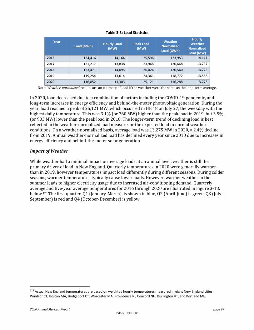
2020 Annual Markets Report page 97 ISO-NE PUBLIC
Table 3-3: Load Statistics
Year
Load (GWh) Hourly Load
(MW) Peak Load
(MW)
Weather Normalized Load (GWh)
Hourly Weather
Normalized Load (MW)
2016 124,416 14,164 25,596 123,953 14,111
2017 121,217 13,838 23,968 120,668 13,737
2018 123,471 14,095 26,024 120,560 13,725
2019 119,254 13,614 24,361 118,772 13,558
2020 116,852 13,303 25,121 116,288 13,275
Note: Weather-normalized results are an estimate of load if the weather were the same as the long-term average.
In 2020, load decreased due to a combination of factors including the COVID-19 pandemic, and long-term increases in energy efficiency and behind-the-meter photovoltaic generation. During the year, load reached a peak of 25,121 MW, which occurred in HE 18 on July 27, the weekday with the highest daily temperature. This was 3.1% (or 760 MW) higher than the peak load in 2019, but 3.5% (or 903 MW) lower than the peak load in 2018. The longer-term trend of declining load is best reflected in the weather-normalized load measure, or the expected load in normal weather conditions. On a weather-normalized basis, average load was 13,275 MW in 2020, a 2.4% decline from 2019. Annual weather-normalized load has declined every year since 2010 due to increases in energy efficiency and behind-the-meter solar generation.
Impact of Weather
While weather had a minimal impact on average loads at an annual level, weather is still the primary driver of load in New England. Quarterly temperatures in 2020 were generally warmer than in 2019, however temperatures impact load differently during different seasons. During colder seasons, warmer temperatures typically cause lower loads. However, warmer weather in the summer leads to higher electricity usage due to increased air-conditioning demand. Quarterly average and five-year average temperatures for 2016 through 2020 are illustrated in Figure 3-18, below.128 The first quarter, Q1 (January-March), is shown in blue, Q2 (April-June) is green, Q3 (July-September) is red and Q4 (October-December) is yellow.
128 Actual New England temperatures are based on weighted hourly temperatures measured in eight New England cities:
Windsor CT, Boston MA, Bridgeport CT, Worcester MA, Providence RI, Concord NH, Burlington VT, and Portland ME.

2020 Annual Markets Report page 98 ISO-NE PUBLIC
Figure 3-18: Seasonal vs. Five-Year Average Temperatures
Quarterly average temperatures in 2020 were either warmer than (Q1 and Q4) or equal to (Q2 and Q3) their historical five–year averages. Q1 and Q4 2020 saw warmer temperatures year-over-year, and warmer temperatures when compared to their historical 5-year average. In Q1 2020, temperatures averaged 36⁰F, a 5⁰F increase compared to Q1 2019 and the warmest Q1 over the last 5 years. Warmer temperatures resulted in 475 fewer Heating Degree Days (HDD) compared to Q1 2019 (2,616 vs. 3,091). In Q4 2020, temperatures averaged 45⁰F, up from 42⁰F in Q4 2019. The warmer temperatures during Q4 2020 were largely a result of warmer weather during November 2020. In November 2020, average temperatures increased 7⁰F year-over-year (46⁰F vs. 39⁰F). HDDs increased by 219 from November 2019 to November 2020. This monthly increase explains 95% of the total quarterly increase of 231 HDDs. Q2 2020 temperatures averaged 57⁰F, while Q3 temperatures averaged 71⁰F. These averages were similar to both the prior year average and 5-year averages.
However, air-conditioning demand in the summer causes a stronger relationship between changes in temperature and load. Temperatures increased year over year in June, August and September, contributing to an increase in Cooling Degree Days (CDD). In those 3 months, CDDs increased by a combined 135, or 98% of the total increase in CDDs for the entire year. The warmer weather during these months, along with increased residential air-conditioning demand during the COVID-19 pandemic helped offset load reductions during other seasons.
Average quarterly load by time of day (hour endings 1-24) is shown in Figure 3-19 below. Temperature changes affect load differently throughout the year. Lower temperatures in the winter (Q1) typically result in higher loads while lower temperatures in the summer (Q3) typically result in less air conditioning demand and therefore lower loads. The shape of the load curve differs by quarter. In the summer, load typically rises throughout the day to a single peak in the late afternoon/early evening, then declines as temperatures decline. When the weather gets colder, there are typically two load peaks: one after the morning ramp, and the second during the evening.
20°
25°
30°
35°
40°
45°
50°
55°
60°
65°
70°
75°
20
16
20
17
20
18
20
19
20
20
20
16
20
17
20
18
20
19
20
20
20
16
20
17
20
18
20
19
20
20
20
16
20
17
20
18
20
19
20
20
Q1 Q2 Q3 Q4
°F
Five-Year Quarterly Average Temperature Quarterly Average Temperature

2020 Annual Markets Report page 99 ISO-NE PUBLIC
Figure 3-19: Average Quarterly Load Curves by Time of Day
Quarterly average load in 2020 was lower than the five-year average in all hours. This tracks accordingly with warmer weather during Q1 and Q4 and the trend of falling wholesale load due to increased energy efficiency and behind-the-meter solar generation. Q1 2020 saw the largest decreases in average hourly load due to the significantly warmer temperatures and the COVID-19 pandemic. In March 2020, state governments began mandating shutdowns to mitigate the spread of COVID-19. This led to lower electricity demand, with average loads decreasing by 936 MW compared to March 2019. While changes (e.g. shutdowns, business closures, people staying home, etc) associated with the COVID-19 pandemic reduced load during most of the year, they also impacted the shape of the average hourly load curve. In Q2 2020, the average hourly load curve peaked in HE 14, two hours later then Q2 2019. The difference is more pronounced during the morning ramp. During HE 8 in Q2 2020, average hourly load decreased by 820 MW compared to HE 8 in Q2 2019 (11,606 MW vs. 12,426 MW). In contrast, average hourly load in HE 19 increased by 75 MW year-over-year (14,100 MW vs. 14,025).
3.4.5 Demand Bidding
The amount of day-ahead cleared demand is significant, because along with the ISO’s Reserve Adequacy Analysis, it influences generator commitment decisions for the operating day.129 In this section, we examine native day-ahead demand cleared (i.e. delivery within the New England jurisdiction, which excludes exports).130 Native demand consists of fixed, price-sensitive, virtual and pumped-storage demand. Fixed demand bids indicate that participants are willing to pay the market-clearing price, regardless of cost. Participants that submit price-sensitive demand bids are
129 The reserve adequacy analysis (RAA) is conducted after the day-ahead market is finalized and is designed to ensure sufficient capacity is available to meet ISO-NE real-time demand, reserve requirements, and regulation requirements. The objective is to minimize the cost of bringing the capacity to the market. For more information see Section 3.4.3
130 Exports are not included as this section focuses on demand participation within New England. Exports are discussed in Section 2.3 and Section 5.
8,000
10,000
12,000
14,000
16,000
18,000
20,000
Q1 Q2 Q3 Q4
MW
2016 2017 2018 2019 2020
Hours of the day (1-24)

2020 Annual Markets Report page 100 ISO-NE PUBLIC
only willing to clear if the market-clearing price is below their bid price. Day-ahead cleared demand by bid type as a percentage of real-time load is shown below in Figure 3-20.131
Figure 3-20: Day-Ahead Cleared Demand as a Percentage of Real-Time Load by Bid Type
Fixed day-ahead cleared demand averaged 61.7% of real-time load in 2020, a 4.0% decrease from 2019 (65.8%). In 2020, price-sensitive demand bids accounted for 35.3% of real-time load, a 3.3% increase from 2019 (31.9%). Lastly, virtual demand as a percentage of real-time load, increased from 2.2% to 2.8% year-over-year. Virtual demand trends are discussed in detail in Section 4.1. Overall, the decrease in fixed demand outweighed the increase price-sensitive demand, and participants cleared slightly less of their real-time load in the day-ahead market compared to 2019 (100.6% vs. 100.9%).
Although price-sensitive demand bids are submitted with a MW quantity and corresponding price, the majority of bids are priced significantly above the LMP. In addition, pumped-storage demand can self-schedule in the day-ahead market. Such transactions are, in practical terms, fixed demand bids. High bid prices are not limited to internal demand bids; Section 5 examines the breakdown between priced and fixed export transactions.
Cleared internal demand bids by price are shown in Figure 3-21 below. The bid prices are shown on the vertical axis, and the percentage of cleared bids that were willing to pay at each bid price are shown on the horizontal axis. For example, over 96% of cleared day-ahead demand was willing to pay more than $155.02/MWh, the maximum day-ahead hub LMP in 2020.
131 Real-time load is the total end-use wholesale electricity load within the ISO New England footprint. Real-time load is equal to Net Energy for Load – Losses.
0%
20%
40%
60%
80%
100%
2016 2017 2018 2019 2020Day
-Ah
ead
Cle
are
d D
em
and
as
a P
erc
en
tage
of
Re
al-
Tim
e M
ete
red
Inte
rnal
De
man
d (
%)
Fixed Demand Price-Sensitive Demand
Pumped Storage Demand Virtual Demand
Uncleared in the Day-Ahead Market

2020 Annual Markets Report page 101 ISO-NE PUBLIC
Figure 3-21: Components of Day-Ahead Cleared Demand as a Percentage of Total Day-Ahead Cleared Demand
Generally, demand in New England is price insensitive. Nearly two-thirds (62%) of total day-ahead cleared demand was bid as fixed demand, so it clears in the market at any price. While price-sensitive demand bids have an attached price, the price is usually above the day-ahead LMP. Therefore price-sensitive demand bids typically clear, accounting for 35% of all day-ahead cleared demand. Virtual demand and price-sensitive pumped-storage demand bids often have lower prices attached to the bid, so they do not clear as often. However, virtual and pumped-storage demand only account for approximately 3% of cleared demand bids.
3.4.6 Load Forecast Error
The ISO produces several different load forecasts, ranging from long-term projections that look out 10 years to short-term forecasts made within the operating day. This section focuses on the day-ahead load forecast: the forecast made around 9:30 am each day that projects hourly load for the next operating day and published on ISO website.132 This forecast is the ISO’s last load projection that is made prior to the close of the day-ahead market. Although the ISO’s forecast is not a direct input into the day-ahead market, it serves as an informational tool for participants bidding in the day-ahead market, and generally aligns well with total day-ahead cleared demand.
Additionally, the reserve adequacy analysis (RAA) process uses the ISO’s load forecasts to make supplemental generator commitment decisions. During the RAA process, the ISO may determine that, based in part on their load forecast, the day-ahead market scheduled insufficient capacity. In these situations, the ISO will commit additional generators over what cleared in the day-ahead market to satisfy real-time load and reserve requirements. These commitments do not happen often, but when they occur, they affect real-time market outcomes.
Just as the day-ahead market cannot perfectly predict real-time conditions, the ISO load forecast will inevitably differ from real-time load. Since weather is both a key driver of load and difficult to
132 Twice a day, the ISO produces a three-day system load forecast that projects load for the current day and the following two days. The first forecast is typically released after 6:00 am and the second and final forecast is the published near 10:00 am.
0% 10% 20% 30% 40% 50% 60% 70% 80% 90% 100%
1000
900
800
700
600
500
400
300
200
100
0
-100
Percentage of Cleared Day-Ahead Demand Bid at Higher Price
Bid
Pri
ce (
$/M
Wh
)
Virtual Demand: 2%
Price Sensitive Demand: 32%
Fixed Demand: 65% of total
Over 96% of cleared demand was bid at a price over $155.02/MWh - the maximum day-ahead LMP in 2020.
Pump StorageDemand: 1%

2020 Annual Markets Report page 102 ISO-NE PUBLIC
predict, real-time load is challenging to forecast. Other factors, such as behind-the-meter solar generation, compound the difficulty of accurately estimating load even in short time horizons.
The mean absolute percent error (MAPE) of the ISO’s day-ahead load forecast (over the past five years) by the time of year is shown in Figure 3-22 below. Months of the year are partitioned into four groups based on the ISO’s monthly load forecast goal (shown as dashed lines). Prior to 2018, the ISO had a MAPE goal of 2.6% for the summer months (June-August) and 1.5% MAPE for the other months.133 In 2018, the ISO revised its goals to 1.5% MAPE in January–April and October–December; 1.8% in May and September; 2.6% remained the goal for months June–August.134
Figure 3-22: ISO Day-Ahead Load Forecast Error by Time of Year
Figure 3-22 shows that forecast error and volatility in 2020 were the highest of the reporting period for each monthly grouping. MAPE, increased between 0.1% (Oct. – Dec.) and 0.7% (May & Sep.) during 2020. Forecast error and volatility increased due to the COVID-19 pandemic. The COVID-19 pandemic initially caused lower loads than the ISO forecasted as state-level mandates led to business closures across the region. During the summer, the COVID-19 pandemic caused higher loads due to residential air conditioning usage.135 At a monthly level, the ISO’s 2020 monthly forecast missed the monthly goal in 6 months, the same number of months as 2018 and 2019 combined. During March and April, the first two months of the COVID-19 pandemic, the ISO’s load forecast missed the monthly goal by 0.8%. These errors were the largest error margins over the last five years.
133 Mean absolute percent error (MAPE) is the average of the hourly absolute percent errors across all hours (on-peak and off-
peak). The absolute percent error is calculated as | ([forecast load] – [actual load]) / [actual load] |.
134 The ISO’s revised the load forecasting goals to account for growing behind-the-meter solar generation which increases the volatility of the load forecast.
135 For more information see the Estimated Impacts of COVID-19 on ISO New England Demand.
0.0%
0.5%
1.0%
1.5%
2.0%
2.5%
3.0%
3.5%
20
16
20
17
20
18
20
19
20
20
20
16
20
17
20
18
20
19
20
20
20
16
20
17
20
18
20
19
20
20
20
16
20
17
20
18
20
19
20
20
Jan-Apr May & Sep Jun-Aug Oct-Dec
Ab
solu
te P
erc
en
t Fo
reca
st E
rro
r (%
)
Interquartile Range MAPE ISO MAPE Goal
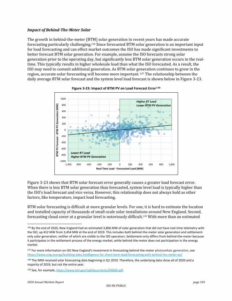
2020 Annual Markets Report page 103 ISO-NE PUBLIC
Impact of Behind-The-Meter Solar
The growth in behind-the-meter (BTM) solar generation in recent years has made accurate forecasting particularly challenging.136 Since forecasted BTM solar generation is an important input for load forecasting and can effect market outcomes the ISO has made significant investments to better forecast BTM solar generation. For example, assume the ISO forecasts strong solar generation prior to the operating day, but significantly less BTM solar generation occurs in the real-time. This typically results in higher wholesale load than what the ISO forecasted. As a result, the ISO may need to commit additional generation. As BTM solar generation continues to grow in the region, accurate solar forecasting will become more important. 137 The relationship between the daily average BTM solar forecast and the system level load forecast is shown below in Figure 3-23.
Figure 3-23: Impact of BTM PV on Load Forecast Error138
Figure 3-23 shows that BTM solar forecast error generally causes a greater load forecast error. When there is less BTM solar generation than forecasted, system level load is typically higher than the ISO’s load forecast and vice versa. However, this relationship does not always hold as other factors, like temperature, impact load forecasting.
BTM solar forecasting is difficult at more granular levels. For one, it is hard to estimate the location and installed capacity of thousands of small-scale solar installations around New England. Second, forecasting cloud cover at a granular level is notoriously difficult.139 With more than an estimated
136 By the end of 2020, New England had an estimated 3,866 MW of solar generation that did not have real-time telemetry with the ISO, up 412 MW from 3,454 MW at the end of 2019. This includes both behind-the-meter solar generation and settlement-only solar generation, neither of which are visible to the ISO operators. Settlement-only differs from behind-the-meter because it participates in the settlement process of the energy market, while behind-the-meter does not participation in the energy market.
137 For more information on ISO New England’s investment in forecasting behind-the-meter photovoltaic generation, see https://www.esig.energy/building-data-intelligence-for-short-term-load-forecasting-with-behind-the-meter-pv/
138 The IMM received solar forecasting data beginning in Q1 2019. Therefore, the underlying data show all of 2020 and a majority of 2019, but not the entire year.
139 See, for example, https://www.bnl.gov/isd/documents/94838.pdf.
-1000
-800
-600
-400
-200
0
200
400
600
800
1000
-1,000 -800 -600 -400 -200 0 200 400 600 800 1,000
BTM
PV
Fo
reca
st -
BTM
PV
Ge
ne
rati
on
(M
W)
Real-Time Load - Forecasted Load (MW)
Higher RT Load Lower BTM PV Generation
Lower RT LoadHigher BTM PV Generation

2020 Annual Markets Report page 104 ISO-NE PUBLIC
4,000 MW of behind-the-meter and settlement-only solar generation, changes in cloud cover or snowfall can have a significant impact on pricing. For example, when less solar generation occurs than what was forecasted, the ISO may need to commit more expensive generators to meet real-time load.
The Interaction between Forecast Error and Pricing Outcomes in 2020
When the ISO’s load forecast differs from real-time load, the forecast error can provide insight into energy market outcomes, including divergence between day-ahead and real-time cleared demand and prices. ISO load forecast error tends to be consistent with the market’s forecast error. That is, when the ISO’s load forecast is greater than actual load, the day-ahead market tends to commit more generation than is required to satisfy actual real-time load. This can result in depressed real-time prices as more expensive generators are backed down from their day-ahead schedules.
Alternatively, when actual loads are greater than the ISO’s forecast, fewer generators are committed in the day-ahead market than are needed in real-time. This can result in real-time prices that are higher than day-ahead prices because more expensive generators (than what cleared in the day-ahead) are required. Often there is a smaller selection of generators to choose from due to start-up time constraints. In such cases, expensive fast-start generators may be required to serve actual load.
The statistical relationship between average daily load forecast error and price divergence is shown in Figure 3-24 below.
Figure 3-24: Price Separation and Forecast Error Relationship
Figure 3-24 illustrates that in 2020 there was a positive correlation between forecast error and price separation between real-time and day-ahead prices. In other words, when real-time loads are higher than day-ahead forecasted demand, real-time prices tend to be higher than day-ahead prices, and vice versa.
-50
-40
-30
-20
-10
0
10
20
30
40
50
-1,000 -800 -600 -400 -200 0 200 400 600 800 1,000
RT
-D
A P
rice
($
/MW
h)
Real-Time Load - Forecasted Load (MW)
Higher RT Load Higher RT Prices
Lower RT LoadLower RT Prices

2020 Annual Markets Report page 105 ISO-NE PUBLIC
3.4.7 Reserve Margin
The reserve margin measures additional available capacity over the load and reserve requirements.140 If the margin is low, the ISO may have to commit additional generators to meet load and reserves, resulting in elevated LMPs. Additionally, the energy market is more susceptible to market power when system conditions are tight.
The annual average margins for each type of reserve requirement and product (10-minute spinning reserve, total 10-minute reserve, and total 30-minute reserve) are shown in Figure 3-25 below. The margins are equal to the actual amount of reserves provided in excess of the corresponding reserve requirement. The total 30 reserve margin surplus is the overall reserve surplus above the total reserve requirement. The total 30 reserve requirement is equal to the total 10-minute reserve requirement, plus 50% of the second largest system contingency. The bars represent the annual average of New England load and total available capacity during the peak hour of each day. The gray bar represents peak load and the orange bar represents average total available capacity.141 Combined, the bars provide context on the difference between load and available capacity during peak hours each year, which is when reserve margins are typically at their lowest.
Figure 3-25: Reserve Margin, Peak Load, and Available Capacity
The average total-10 minute margin fell by 250 MW, from 3,920 MW in 2019 to 3,670 in 2020. The decline in the total 10-minute reserve margin led to a slight increase in 10-minute non-spinning reserve pricing (discussed further in Section 7.1). The primary driver was a 330 MW decline in reserves from pumped-storage generators, from 1,190 MW (70% of total 10-minute requirement) in 2019 to 860 MW (50% of total 10-minute requirement) in 2020, on average. The flexibility of pumped-storage generators allows them to cycle online and offline quickly. Since one pumped-
140 The reserve margin is the difference between available capacity and demand. The equations below illustrate this
relationship: i. 𝐺𝑒𝑛𝐸𝑛𝑒𝑟𝑔𝑦 + 𝐺𝑒𝑛𝑅𝑒𝑠𝑒𝑟𝑣𝑒𝑠 + [𝐼𝑚𝑝𝑜𝑟𝑡𝑠 − 𝐸𝑥𝑝𝑜𝑟𝑡𝑠] = 𝐷𝑒𝑚𝑎𝑛𝑑 + [𝑅𝑒𝑠𝑒𝑟𝑣𝑒 𝑅𝑒𝑞𝑢𝑖𝑟𝑒𝑚𝑒𝑛𝑡]. Equation i. is
equivalent to: 𝑆𝑢𝑝𝑝𝑙𝑦 + 𝐺𝑒𝑛𝑅𝑒𝑠𝑒𝑟𝑣𝑒𝑠 − [𝑅𝑒𝑠𝑒𝑟𝑣𝑒 𝑅𝑒𝑞𝑢𝑖𝑟𝑒𝑚𝑒𝑛𝑡] = 𝐷𝑒𝑚𝑎𝑛𝑑 or 𝑆𝑢𝑝𝑝𝑙𝑦 + 𝑅𝑒𝑠𝑒𝑟𝑣𝑒 𝑀𝑎𝑟𝑔𝑖𝑛 = 𝐷𝑒𝑚𝑎𝑛𝑑
141 Available capacity is the generation capacity that can be delivered within a 30 minute period: 𝐺𝑒𝑛𝐸𝑛𝑒𝑟𝑔𝑦 + 𝐺𝑒𝑛𝑅𝑒𝑠𝑒𝑟𝑣𝑒𝑠 +
[𝐼𝑚𝑝𝑜𝑟𝑡𝑠 − 𝐸𝑥𝑝𝑜𝑟𝑡𝑠]
0
5,000
10,000
15,000
20,000
25,000
0
500
1,000
1,500
2,000
2,500
3,000
3,500
2016 2017 2018 2019 2020
Pe
ak L
oad
an
d A
vaila
ble
Cap
acit
y M
W
Re
serv
e M
argi
n M
W
Peak Load (Right Axis) Available Capacity (Right Axis)
Total30 Reserve Margin Total10 Reserve Margin
Total10Sping Reserve Margin

2020 Annual Markets Report page 106 ISO-NE PUBLIC
storage generator was on planned long-term outage, the remaining pumped-storage generators were called upon more frequently, and thus could not provide 10-minute non-spinning reserves. The largest change outside of pumped-storage generators were several newly commissioned natural gas-fired generators that contributed 70 MW more to the total-10 minute requirement in 2020 (200 MW) compared to 2019 (130 MW), on average.
3.4.8 System Events during 2020
Despite certain days where storms or unplanned outages affected the system, conditions were relatively benign in 2020, with no shortage events or instances of prolonged cold or hot temperatures.
The following metrics illustrate the frequency of abnormal system conditions and extreme market outcomes over the past five years:
Number of OP4 and M/LCC 2 Events Reserve Deficiency Events Instances of High Pricing measured by Implied Heat Rates
OP 4 and M/LCC 2 Events
The ISO uses the following established procedures to alert participants and relieve issues during times of tight or abnormal system conditions:
Master Local Control Center Procedure No. 2 (M/LCC 2, Abnormal Conditions Alert)142 notifies market participants and power system operations personnel when an abnormal condition is affecting the reliability of the power system, or when such conditions are anticipated. The ISO expects these entities to take certain precautions during M/LCC 2 events, such as rescheduling routine generator maintenance to a time when it would be less likely to jeopardize system reliability.
Operating Procedure No. 4 (OP-4, Action during a Capacity Deficiency)143 establishes criteria and guidelines for actions during capacity deficiencies. There are eleven actions described in the procedure which the ISO can invoke as system conditions worsen.
The number of instances for each type of event during the reporting period is detailed in Table 3-4 below.
142 Information on individual M/LCC 2 events is available at:
https://www.iso-ne.com/static-assets/documents/2016/02/mlcc_2_20111219_to_20160105.xlsx
143 See ISO New England Operating Procedure No. 4 – Action During A Capacity Deficiency, available at
https://www.iso-ne.com/static-assets/documents/rules_proceds/operating/isone/op4/op4_rto_final.pdf

2020 Annual Markets Report page 107 ISO-NE PUBLIC
Table 3-4: OP-4 and M/LCC 2 Event Frequency
2016 2017 2018 2019 2020
# of OP-4 Events 1 0 1 0 0
# of M/LCC 2 Events 4 7 7 0 3
The ISO implemented three M/LCC 2 events in 2020. The events occurred due to the threat of severe storms that struck the region in April, August, and October. The August event was the most notable. M/LCC 2 was in effect from August 4 to August 10 due to tropical storm Isaias, which caused customer power outages as well as unplanned generator and transmission outages. At the peak of the storm on the evening of August 4, about 1.2 million customers were without power. The majority of customer outages occurred in Connecticut. The storm and customer outages also resulted in large load forecast errors. Actual loads were 3,944 MW (20%) less than the forecast on the evening of August 4, resulting in lower real-time LMPs. There were no OP-4 events in 2020.
Negative Reserve Margins
Negative reserve margins are an indicator of stressed system conditions. In these instances, the system does not have enough available supply to meet the reserve requirements necessary to maintain system reliability. In particular, negative non-spinning reserve margins result in very high real-time energy prices, because reserve prices reach the Reserve Constraint Penalty Factor (RCPF) prices of $1,000 for thirty minute operating reserve (TMOR) and/or $1,500 for ten-minute non-spinning reserve (TMNSR).144 The number of hours with negative non-spinning and spinning reserve margins are presented in Table 3-5 below.
Table 3-5: Frequency of Negative Reserve Margins (System Level) 145
Year Hours of Negative Total30 Margins
Hours of Negative Total10 Margins
Hours of Negative Total10Spin Reserve
Margins
2016 3.2 0.3 37.8
2017 0.6 0.0 57.0
2018 2.7 0.9 68.1
2019 0.0 0.0 25.9
2020 0.0 0.0 14.4
Unlike the first three years in the reporting period, there was always a surplus of TMNSR and TMOR in 2019 and 2020. Additionally, spinning reserve shortages were less frequent in 2020 than in every other year in the reporting period. The spinning reserve shortages occurred across 31 days throughout the year in 2020 due to a variety of factors, such as tight system conditions caused by higher real-time loads or unplanned outages.
144 Section 7.1.1 provides additional information on Reserve Constraint Penalty Factors.
145 The calculations in this table come from the pricing and LMP calculation processes in the real-time market software. The “Hours of Negative Total30 Margins” column does not include instances where only the replacement reserve margin is negative, because those instances are not associated with the high $1,000/MWh and $1,500/MWh RCPFs.

2020 Annual Markets Report page 108 ISO-NE PUBLIC
Frequency of extreme energy prices at the Hub
High real-time LMPs can indicate stressed system conditions, as higher-cost generation is required to meet load and reserve requirements. The duration curves in Figure 3-26 below show the top 1% of hourly real-time LMPs ranked from high to low over the past five years.
Figure 3-26: LMP Duration Curves for Top 1% of Real-Time Hours
This figure shows that 2020 real-time Hub LMPs were lower than in any other year in the reporting period across the top 1% of ranked observations. This trend persisted across the remaining 99% of observations. Real-time LMPs were also relatively low in 2019 compared to the previous three years. In 2016-2018, there were periods of tight system conditions that resulted in high non-spinning reserve pricing and high LMPs. No comparable events occurred in 2020 or 2019.
Market Performance during system events in May 2020
The unexpected loss of a generator or transmission equipment can have a significant impact on energy market outcomes. A series of outage events at the end of May 2020 bear specific mention.
Overview of Events: The timeline of events on May 27, May 29, and May 30 is described below.
May 27
The Phase II interconnection with Hydro Quebec went off-line just before 3pm due to a lightning strike, resulting in the unexpected loss of 1,890 MW of energy imports into New England.
In addition, expected net imports over the New York North interface were also reduced (relative to the day-ahead cleared quantity), decreasing net imports into New England to almost 0 MW between 2pm and 4pm.
Phase II returned to service later that evening at 6pm.
May 29
-200
0
200
400
600
800
1,000
1,200
1,400
1,600
1,800
2,000
2,200
2,400
0.0% 0.5% 1.0%
$/M
Wh
2016 2017 2018 2019 2020
2020 LMPs were lower than those of 2016-2019 across all ranked observations
Highest 2020 value:LMP = $236/MWh
Highest 2019 value:LMP = $261/MWh

2020 Annual Markets Report page 109 ISO-NE PUBLIC
The ISO experienced a loss of 1,250 MW due to an unexpected nuclear generator outage just after 2pm.
At 8:30pm, the Phase II interconnection unexpectedly failed due to an equipment issue, resulting in a loss of 1,340 MW.
May 30
Phase II partially returned around 12pm. The nuclear generator remained out of service until June 1, despite having a day-ahead
schedule for May 30.
Although the unexpected losses of energy on both occasions was relatively large (in the 2-2.5 GW/hour range), the ISO’s real-time energy market did not experience a capacity scarcity event, and the ISO did not implement M/LCC2 or OP4 protocols.146,147,148 On both May 27 and May 29, conditions were relatively stable before the supply losses occurred, and the system was able to recover from the losses quickly. The ISO committed additional generators in real-time in response to the unexpected losses of energy. On average, the additional real-time generation commitments were smaller in magnitude than the supply losses, due to additional real-time energy from self-scheduled generation and settlement-only generation. Further, spinning reserve margins remained at low to normal values, indicating that there was no notable excess of online generation. To ensure the availability of total 10-minute operating reserves, the ISO instructed several pumped-storage generators to go (or remain) off-line on May 30. These units received a total of $105,000 in uplift payments during the hours that they were postured. No other types of generators were held back to provide reserves during the system events.
The timing and magnitude of these unexpected supply losses are illustrated in Figure 3-27 below. To ensure the reliability of the transmission system during these substantial supply losses, the ISO’s market software and Reserves Adequacy Analysis (RAA) process committed additional generators to provide both energy and reserves. These commitments included both fast-start generators that could come on-line quickly (within 10 or 30 minutes, red shading in figure) and longer-lead-time generators that were supplementally committed on May 29 (several hours after the initial recoveries) and May 30 (green shading).149
146 A capacity scarcity event occurs when the system or local area is short on 10- and/or 30-minute non-spinning reserves, and the reserve constraint penalty factor for one or more of these non-spinning products is setting the real-time reserve price.
147 When notified of an M/LCC 2 Abnormal Conditions Alert, applicable power system personnel and market participants are expected to take precautions so that routine maintenance, construction or test activities do not further jeopardize the reliability of the power system.
148 Operating Procedure #4 establishes criteria and guidelines for actions during a capacity deficiency, as directed by the ISO and as implemented by ISO and the Local Control Centers (LCCs). 149 Supplementally-committed generators refer to longer-lead-time generators committed after the day-ahead market had closed.

2020 Annual Markets Report page 110 ISO-NE PUBLIC
Figure 3-27: Real-Time Hourly Supply Composition on May 27, 29 and 30150
Though supplemental commitments began later in the day on May 29, fast-start generators committed by the market software responded to the immediate energy losses after the major trips on May 27 and 29. During the periods with large unexpected supply reductions, the market software and RAA processes committed an average of 1,600 MW per hour of additional energy. The supply committed to offset the losses came exclusively from generators, with no significant supply commitment from demand response resources. Market Outcomes: The major supply losses on May 27, 29, and 30 resulted in high energy prices. During several pricing intervals over the time period, reserve prices contributed to higher real-time LMPs. The real-time Hub LMP and system level reserve price for each product are shown at the five-minute level in Figure 3-28 below.
150 Reduction in net imports from New York North is relative to the day-ahead cleared quantity.
0
2,000
4,000
6,000
8,000
10,000
12,000
14,000
16,000
18,000
May 27 May 29 May 30
MW
pe
r H
ou
r
Nuclear Net Imports Other Generation Supply RT Supplemental RT Fast Start
Unplanned Nuclear Outage Phase II Failure
ISO RT Supply Additions
Phase II Failure & Reduction in Importsfrom New York North

2020 Annual Markets Report page 111 ISO-NE PUBLIC
Figure 3-28: Five-Minute Real-Time Hub LMPs and Rest-of-System Reserve Prices
Five-minute real-time energy prices peaked at $183.93/MWh around 5pm on May 27 and at $224.46/MWh at 12:30am on May 30. Reserve prices peaked at $129.32/MWh on May 27 and at $50/MWh on May 29 and 30. Though redispatch was needed to procure additional non-spinning reserves on May 27, the system did not become deficient in non-spinning reserves, and the reserve constraint penalty factors (RCPFs) for the 10- and 30-minute non-spinning products did not bind. For reference, during the capacity scarcity event that occurred on September 3, 2018, deficits triggered RCPFs and reserve prices reached $2,500/MWh. Real-time first contingency uplift payments during hours affected by the system events (i.e., hours ending 16-18 on May 27, and hour ending 15 on May 29 through hour ending 24 on May 30) totaled $381,000. The following bullet points describe the breakdown of categories included in the $381,000 total. Out-of-merit payments ($161,000, 42%): Out-of-merit uplift is the traditional form of
uplift, and is paid to generators when market revenues are insufficient to cover their as-bid commitment and dispatch costs.
Posturing payments ($105,000, 28%): Posturing uplift payments restore profits foregone by resources when the ISO instructs them to stop producing energy. This helps ensure that postured resources will follow the ISO’s dispatch instructions. During this event, pumped-storage generators were the only type of resource that was postured.
Dispatch LOC payments ($56,000, 15%) and RRP payments ($58,000, 15%): Similar to posturing payments, dispatch LOC and RRP payments result from the ISO instructing a generator to operate at a level other than its economic dispatch point. Both types of payments restore opportunity costs incurred by generators when following the ISO’s dispatch instructions.
0
50
100
150
200
250
May 27 May 29 May 30
$/M
Wh
Real-Time Hub LMP TMSR Price TMNSR Price TMOR Price
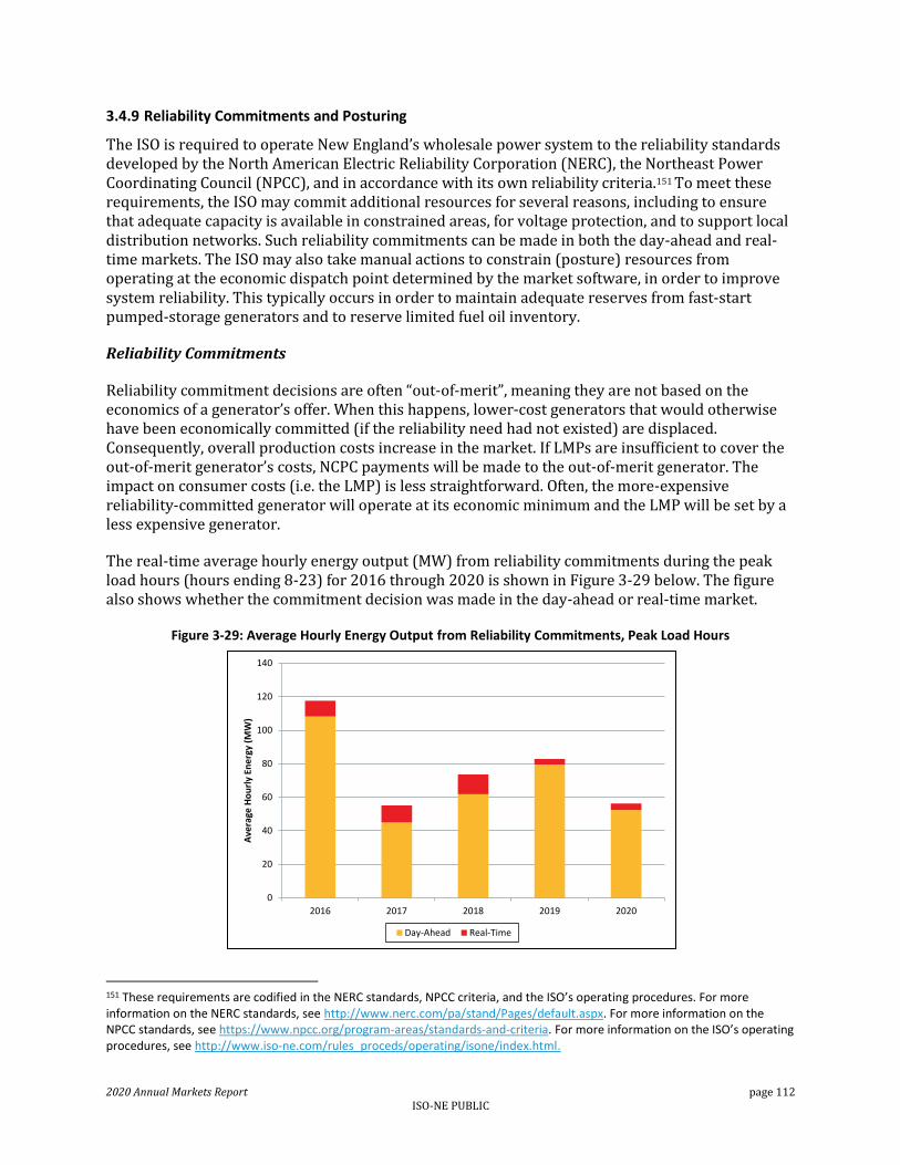
2020 Annual Markets Report page 112 ISO-NE PUBLIC
3.4.9 Reliability Commitments and Posturing
The ISO is required to operate New England’s wholesale power system to the reliability standards developed by the North American Electric Reliability Corporation (NERC), the Northeast Power Coordinating Council (NPCC), and in accordance with its own reliability criteria.151 To meet these requirements, the ISO may commit additional resources for several reasons, including to ensure that adequate capacity is available in constrained areas, for voltage protection, and to support local distribution networks. Such reliability commitments can be made in both the day-ahead and real-time markets. The ISO may also take manual actions to constrain (posture) resources from operating at the economic dispatch point determined by the market software, in order to improve system reliability. This typically occurs in order to maintain adequate reserves from fast-start pumped-storage generators and to reserve limited fuel oil inventory.
Reliability Commitments
Reliability commitment decisions are often “out-of-merit”, meaning they are not based on the economics of a generator’s offer. When this happens, lower-cost generators that would otherwise have been economically committed (if the reliability need had not existed) are displaced. Consequently, overall production costs increase in the market. If LMPs are insufficient to cover the out-of-merit generator’s costs, NCPC payments will be made to the out-of-merit generator. The impact on consumer costs (i.e. the LMP) is less straightforward. Often, the more-expensive reliability-committed generator will operate at its economic minimum and the LMP will be set by a less expensive generator.
The real-time average hourly energy output (MW) from reliability commitments during the peak load hours (hours ending 8-23) for 2016 through 2020 is shown in Figure 3-29 below. The figure also shows whether the commitment decision was made in the day-ahead or real-time market.
Figure 3-29: Average Hourly Energy Output from Reliability Commitments, Peak Load Hours
151 These requirements are codified in the NERC standards, NPCC criteria, and the ISO’s operating procedures. For more information on the NERC standards, see http://www.nerc.com/pa/stand/Pages/default.aspx. For more information on the NPCC standards, see https://www.npcc.org/program-areas/standards-and-criteria. For more information on the ISO’s operating procedures, see http://www.iso-ne.com/rules_proceds/operating/isone/index.html.
0
20
40
60
80
100
120
140
2016 2017 2018 2019 2020
Ave
rage
Ho
url
y En
erg
y (M
W)
Day-Ahead Real-Time

2020 Annual Markets Report page 113 ISO-NE PUBLIC
Reliability commitments remain a relatively small component of total system generation, at less than 0.3%, on average. Over the review period, reliability commitments were relatively low, averaging 77 MW per hour. The average hourly energy of ISO reliability commitments decreased from 83 MW per hour in 2019 to 56 MW per hour in 2020. Commitments in the day-ahead market have become more common as a percentage of total reliability commitments.
In 2020, the vast majority (87%) of reliability commitments occurred for Local Second Contingency Reliability Protection (LSCPR). Special-Constraint Resources (SCR) and voltage support resources accounted for 3% and 9% of reliability commitment resources, respectively.152 Almost three quarters of all reliability commitments (74%) occurred in Maine and SEMA-RI; the remainder were in NEMA (10%) and New Hampshire (15%). These reliability commitments primarily reflected a need for additional on-line generation in areas with transmission upgrades and outages, to ensure local reliability.
In 2019, 94% (79.2 MW/hr average) of the output from reliability commitments was for Local Second Contingency Reliability Protection (LSCPR), with 56% (45 MW/hr) of LSCPR commitments in Maine and 27% in SEMA (22 MW/hr). Voltage support commitments represented a relatively small percentage of overall reliability commitments and, in 2019, accounted for just 2.8% of reliability commitments (2.4 MW/hr). The increase in overall reliability commitments in 2019 resulted from local reliability commitments in Maine and SEMA between May and December, to support planned transmission work.
The 2018 increase in reliability commitments, compared to 2017, resulted from outages during transmission upgrade work in the NEMA/Boston, Rhode Island and SEMA zones. The reduction in reliability commitments after 2016 reflected the completion of planned transmission work that required must-run generation in the Boston area. Prior to the completion of the upgrades, the Boston area necessitated regular reliability commitments to reliably satisfy load in the Boston area.
A monthly breakdown of reliability commitments made during 2020 is shown in Figure 3-30 below. The figure shows the out-of-rate energy for reliability commitments during the peak load hours in 2020, by market and month. Out-of-rate energy includes reliability commitment output that is offered at a higher price than the LMP, and, therefore, would not likely have been committed or dispatched in economics.
152 An explanation for the reliability commitment types may be found here: https://www.iso-ne.com/participate/support/glossary-acronyms/

2020 Annual Markets Report page 114 ISO-NE PUBLIC
Figure 3-30: Day-Ahead and Real-Time Average Out-of-Rate Energy from Reliability Commitments, Peak Load Hours, 2020
Of the roughly 56 MW of average hourly output from generators committed for reliability, about 26 MW (on average) was out-of-rate. This is a relatively small amount of out-of-rate energy (in the context of average hourly load of over 13 GW in 2020) that was served by more expensive generation to meet a reliability need. Figure 3-30 shows that the greatest amount of out-of-rate energy from reliability commitments occurred from August to December; these commitments supported planned transmission outages in Maine and SEMA-RI. The LSCPR reliability commitments explain the pattern and magnitude of the out-of-rate commitments. As noted earlier, approximately 87% of all reliability commitments were for LSCPR in 2020.153 Total LSCPR NCPC payments in 2020 were approximately $4 million; while this represented 16% of total uplift payments for the year, it represented just 0.1% of total energy payments.
As shown in the two figures above, a large majority of the 2020 reliability commitments were made in the day-ahead market. This helps minimize surplus capacity and the amount of economic generation that is displaced in the real-time operating day. If a reliability requirement is known prior to the clearing of the day-ahead market, commitments can be made in the day-ahead market to meet the requirement.
Committing generators in the day-ahead market is more desirable than commitments later in the Reserve Adequacy Analysis (RAA) process or in real-time as day-ahead commitments tend to reduce the risk of suppressed real-time prices and higher NCPC payments. If reliability commitments are known in the day-ahead market, the commitment schedules of other generators can be adjusted to accommodate the reliability commitment. This provides more flexibility than if the commitment is made later, reducing the risk of having excess inflexible supply online. Excessive generator commitments can distort prices by removing other generators from the supply stack and adding fixed energy to the supply stack. The excess fixed supply could potentially suppress real-time prices and increase NCPC.
Posturing Actions
153 Local second contingency protection reliability (LSCPR) commitments are made for import-constrained subareas, if necessary, to ensure that the ISO can re-dispatch the system to withstand a second contingency loss within 30 minutes after the first contingency loss without exceeding transmission element operating limits.
0
10
20
30
40
50
60
70
80
90
Jan Feb Mar Apr May Jun Jul Aug Sep Oct Nov Dec
2020
Ave
rage
Ho
url
y En
erg
y (M
W)
Day-Ahead Hourly Out-of-Rate MWs Real-Time Hourly Out-of-Rate MWs

2020 Annual Markets Report page 115 ISO-NE PUBLIC
In addition to committing off-line, out-of-merit generators to ensure local reliability, the ISO may limit the output of potentially in-merit generators to ensure either system-wide or local reliability. Limiting the output of generators is called “posturing.” Posturing generators results in the preservation of fuel for “limited energy” generators, allowing fuel to be used later in the event of system contingencies. Generators may be postured either on-line or off-line. When generators are postured on-line, it is often at the generator’s economic minimum; the generator provides operating reserves while postured, but is only available for manual dispatch above the posturing level in the event of a system contingency. Generators postured off-line also provide either 10- or 30-minute operating reserves, if fast-start capable.
Because posturing removes potentially in-merit generation from economic dispatch, postured generators may be financially worse-off as a result of the ISO’s actions, unless the ISO provides uplift payments to compensate for foregone profitable dispatch. Postured generators may receive NCPC for any foregone profits that occurred during the posturing period. Generally, the postured generator’s remaining energy is compared to its economic dispatch opportunities during the posturing period. NCPC is provided for the net profits of optimal economic dispatch that would have occurred absent posturing, compared to the profitability of the actual dispatch that occurred during the posturing period.154
Postured energy (GWh) and NCPC payments by month are shown in Figure 3-31 below.155 The bars indicate the postured energy obtained (the amount of energy constrained down) from pumped-storage generators and all other types of generators.156
Figure 3-31 Monthly Postured Energy and NCPC Payments
154 See Market Rule 1, Appendix F, Sections 2.3.8 and 2.3.9.
155 Postured energy is the amount of energy that is unavailable for economic dispatch, given the posturing action; this value is used in the settlement compensation for the posturing action.
156 Very infrequently, pumped-storage demand (or asset-related demand) is postured. These resources are postured on-line (in consumption mode) to increase operating reserves. The energy associated with these posturing activities is not depicted in the figure.

2020 Annual Markets Report page 116 ISO-NE PUBLIC
As indicated in the figure above, pumped-storage generators are frequently postured throughout the year. In 2020, only pumped-storage generators were postured, and posturing levels were relatively low, at 12 GWh in total, compared other years in the review period.157 Only in January 2018 have non-pumped-storage generators been postured. The posturing in January 2018 involved a number of oil-fired generators, with limited fuel, being postured during a prolonged cold snap period that resulted in significant concerns about the day-to-day availability of natural gas for electric generation. The postured oil-fired generators were effectively providing back-up electricity supply, in the event of a natural gas shortage during the cold snap.
As indicated in the figure, NCPC payments to postured generators were quite low throughout 2020, with approximately $0.5 million in total payments (accounting for 1.8% of all NCPC payments in 2020). NCPC payments were highest during January 2018, when the cold snap period resulted in significant posturing of oil-fired generators. While the magnitude of NCPC payments is generally consistent with the quantity of energy being postured, posturing during very high energy price periods also can result in high NCPC payments, even when the postured energy quantity is not extremely large. This occurs because the postured generators forgo the high LMPs and must be compensated for lost profits. This is noticeable in August 2016, when pumped-storage generators were postured on August 11, during a capacity deficiency period (Operating Procedure 4) with operating reserve deficiencies and very high energy prices.
3.4.10 Congestion
This section provides an overview of how congestion occurs in an electrical transmission system and how it affects LMPs. It then compares the amount of congestion in New England in 2020 against historical levels of congestion over the last five years. In general, New England has experienced low levels of congestion in recent years. One prominent trend over this period has been the shift between generation and load in terms of who is paying congestion costs, with generation paying a larger share of these costs every year over the reporting period. This is partly the result of the New England transmission system becoming more export constrained in recent years. Subsequently, this section explores where congestion occurred geographically in the New England transmission system in 2020. It concludes by looking at some of the most frequently binding transmission constraints in New England in 2020.
Overview of Congestion
At every node in the New England power system, LMPs reflect the cost of delivering the next megawatt (MW) of energy at the lowest cost to the system. The LMP is comprised of three components: the energy component, the congestion component, and the loss component. The energy component is the same for all locations in the power system. The congestion component reflects the additional system costs when transmission constraints prevent the use of the least-cost generation to meet the next increment of load. The loss component reflects the dispatch of additional generation because some electric energy is lost during transmission. Breaking down the LMP into these components enables the ISO to determine how much of the difference in LMPs at two locations is due to transmission congestion versus losses. Locational differences in the congestion component serve as the basis for determining the value of financial transmission rights (FTRs), a financial instrument that market participants can use to hedge transmission congestion cost risk. FTRs are covered in more detail in Section 4.2.
157 For context, the total supply/load in 2020 was approximately 117,000 GWh.

2020 Annual Markets Report page 117 ISO-NE PUBLIC
The physical limits of transmission elements are modeled as constraints in the economic optimization that the ISO administers to determine the least-cost way of producing electricity. When the power flowing through a transmission element reaches its limit, the constraint associated with that transmission element is said to “bind.” When this happens, the transmission system has limited the extent to which the least-expensive generation can meet load in the system. In this situation, higher-cost generation must be dispatched in the constrained area, which raises the price of energy in that area. Locational difference in prices caused by a binding transmission constraint are reflected in the LMP through the congestion component. The congestion component can be positive or negative. A negative congestion component indicates an export-constrained area (i.e., areas where there is an imbalance of generation relative to load and there is insufficient transmission capability to export the excess energy), and a positive congestion component indicates an import-constrained area (i.e., areas where there is an imbalance of load relative to generation and there is insufficient transmission capability to import the additional needed energy).
Cost of Congestion
One way to explore the financial impact of congestion is to analyze congestion charges and credits. The ISO settles the day-ahead and real-time energy markets by calculating charges and credits for all market activity that occurs at each pricing location (node) in the system. Energy market settlement is performed on each of the three components of the LMP separately. By design, the congestion credits and charges do not balance; the charges are expected to exceed the credits. The surplus revenue is called congestion revenue. Congestion revenue is collected in both the day-ahead and real-time energy markets and it forms the basis of the congestion revenue fund, which is used to pay the holders of FTRs.
The congestion charges and credits for the day-ahead energy market for the last five years are shown in Figure 3-32 below. In this figure, charges are shown as positive values, while credits are shown as negative values. This chart also illustrates the sum of the congestion charges and credits (i.e., the day-ahead congestion revenue) each year using white diamonds. Further, this chart depicts the congestion credits and charges associated with the different categories that constitute day-ahead generation obligation (DAGO), day-ahead load obligation (DALO), and day-ahead demand reduction obligation.158,159
158 See Market Rule 1 Sections III.3.2.1 (a) (i), (ii), and (iii) for more information about DAGO, DALO, and day-ahead demand reduction obligation. Also, see Market Rule 1 Section III.3.2.1 (f) for information about how day-ahead market charges and credits are determined. In Figure 3-32, cleared demand bids have been categorized as either locational demand or asset-related demand (ARD); cleared supply offers have been labeled generation, and day-ahead demand reduction obligation is labeled as demand reduction.
159 Figure 3-32 does not include day-ahead energy internal bilateral transactions (IBTs). This reflects a change in how this figure was presented in the 2019 Annual Markets Report. Day-ahead IBTs are contracts between two market participants in which the “buyer” receives a reduction in its day-ahead and real-time adjusted load obligation of the MW amount listed in the contract and the “seller” receives an increase in its day-ahead and real-time adjusted load obligation for the same MW amount. Because these transactions are balanced, day-ahead IBTs do not have a net impact on the day-ahead congestion revenue fund.

2020 Annual Markets Report page 118 ISO-NE PUBLIC
Figure 3-32: Day-ahead Energy Market Congestion Charges and Credits
Day-ahead congestion charges totaled $45.4 million in 2020, their lowest level of the last five years. This represents a 7% decrease from the $49.0 million participants paid in day-ahead congestion charges in 2019. Meanwhile, day-ahead congestion credits totaled $15.7 million in 2020. This represents an 8% increase from the $14.6 million participants received in the day-ahead market in 2020. In total, the day-ahead congestion revenue in 2020 (white diamond) amounted to $29.7 million, which represents a 14% decrease from the day-ahead congestion revenue in 2019 ($34.4 million). Day-ahead congestion revenue reached its peak value over the five-year reporting horizon in 2018, when significant congestion occurred at New York – New England (NYNE) interface and resulted in imports paying elevated congestion charges.
The decrease in congestion charges between 2019 and 2020 was particularly notable for imports. The day-ahead generation obligation category paid 38% less in congestion charges in 2020 than in 2019, as their charges decreased from $20.0 million to $12.5 million. Meanwhile, day-ahead congestion charges increased for generation and virtual supply. Charges to generation rose by 25% (from $17.4 million in 2019 to $21.7 million in 2020), while charges to virtual supply increased by 7% (from $4.5 million in 2019 to $4.8 million in 2020). Day-ahead generation obligation incurs congestion charges when it receives a reduced price for its energy as a result of a negative congestion component at the location where it is supplying energy.
Congestion charges decreased for locational demand (i.e., demand that is not virtual, an export, or associated with asset-related demand) between 2019 and 2020. The congestion charges to locational demand shrank by 9%, falling from $6.8 million in 2019 to $6.2 million in 2020. The change in congestion charges to the other categories of day-ahead load obligation were all quite small in magnitude, each changing by less than $0.1 million from the prior year. Collectively, congestion charges to virtual demand, exports, and asset-related demand accounted for only 0.6% of all congestion charges in 2020. Day-ahead load obligation incurs congestion charges when it has to pay more for its energy as a result of a positive congestion component at the location where it is assuming the load obligation.
Over the last five years, load has paid an increasingly smaller share of congestion costs in the day-ahead market relative to generation. This can be seen in Figure 3-33 below which shows the share
$34 $39
$68
$34 $30
(60)
(40)
(20)
0
20
40
60
80
100
120
2016 2017 2018 2019 2020
Day
-Ah
ead
Co
nge
stio
n C
har
ges
and
Cre
dit
s($
mill
ion
s)
Generation Virtual Supply Import
ARDs Locational Demand Virtual Demand
Exports Demand Reduction DA Congestion Revenue
Charges
Credits

2020 Annual Markets Report page 119 ISO-NE PUBLIC
of day-ahead congestion costs that are paid by day-ahead generation obligation (green), day-ahead load obligation (purple), and day-ahead demand reduction obligation (red).160
Figure 3-33: Percent of Day-ahead Energy Market Congestion Costs Paid by Category
In 2020, load paid only 14% of day-ahead congestion costs; this is tied with 2019 for the smallest share paid over the reporting period. In contrast, load paid 33% of day-ahead congestion costs in 2016. The share of day-ahead congestion costs paid by load has decreased every year, while the share of these costs paid by generation has increased every year. In 2016, generation paid 67% of day-ahead congestion costs, while in 2020 that share grew to 86%. This shift of congestion costs between load and generation is reflective of a transmission system in New England that has evolved from one that was more import-constrained to one that is now more export-constrained. This change is also evident in Table 3-6, which appears toward the end of this section. This table shows that almost all of the most frequently binding interface constraints in the day-ahead market in 2020 were export constraints.
Congestion relative to Energy Market Payments
Over the last five years, congestion revenue has been small relative to total energy market payments. This can be seen in Figure 3-34 below, which shows the congestion revenue in New England by market and year between 2016 and 2020. The purple bars represent the day-ahead congestion revenue, and the green bars represent the real-time congestion revenue. Bars with a positive value indicate that the congestion charges exceeded the congestion credits for that year in that market, while bars with a negative value indicate that congestion credits exceeded the congestion charges. The percentages in the figure are the total congestion revenue each year expressed as a percent of total energy market costs.
160 The day-ahead congestion costs paid by day-ahead demand reduction obligation are so small – amounting to less than twenty thousand dollars in the last five years – that they are not visible in the figure.
67%78% 82% 86% 86%
33%
22% 18% 14% 14%
0%
10%
20%
30%
40%
50%
60%
70%
80%
90%
100%
2016 2017 2018 2019 2020
Shar
e o
f D
ay-A
he
ad C
on
gest
ion
Co
sts
DAGO DALO Demand Reduction

2020 Annual Markets Report page 120 ISO-NE PUBLIC
Figure 3-34: Congestion Revenue Totals and as Percent of Total Energy Cost
Total day-ahead and real-time congestion revenue was $29.1 million in 2020. This represents a 12% decrease from $32.9 million dollars in 2019. The congestion revenue in 2020 represents less than 1% of total energy costs (labels), which was comparable to other years in the reporting period. The majority of the congestion revenue came from the day-ahead market. Because the real-time market is a balancing market, the congestion that occurs in real-time only affects deviations from day-ahead schedules. Consequently, the magnitude of congestion revenue in the real-time market is small relative to the congestion revenue in the day-ahead market. In 2020, the real-time congestion revenue amounted to -$0.6 million, while the day-ahead congestion revenue totaled $29.7 million.
Congestion Patterns in New England
The New England nodes most affected by transmission congestion in the day-ahead market in 2020 are shown in Figure 3-35 below.161 The colors of the nodes are indicative of the average day-ahead congestion component in 2020. Blue dots represent locations that had an average day-ahead congestion component that was negative in 2020. The darker the blue, the lower the average day-ahead congestion component (i.e. more export-constrained or more negative the congestion component). These nodes are in export-constrained areas. Red dots represent locations that had an average day-ahead congestion component that was positive in 2020. These nodes are in import-constrained areas.
161 This figure only includes nodes that had an average day-ahead congestion component of greater than or equal to $0.10/MWh or less than or equal to -$0.10/MWh in 2020.
0.94%0.92%
1.06%
0.80%0.96%
(10)
0
10
20
30
40
50
60
70
80
2016 2017 2018 2019 2020
Co
nge
stio
n R
eve
nu
e
($ m
illio
ns)
Day-Ahead Congestion Revenue Real-time Congestion Revenue
% - Percent of Total Energy Cost

2020 Annual Markets Report page 121 ISO-NE PUBLIC
Figure 3-35: New England Pricing Nodes Most Affected by Congestion, 2020
Several patterns of congestion have been highlighted in Figure 3-35 and each of them is discussed in detail below:
1) Northern Maine, New Hampshire, and Vermont: As has been the case for the last several years, areas in northern Maine, New Hampshire, and Vermont were frequently export-constrained in 2020. These are areas on the system with a high concentration of intermittent (predominantly wind) generators. Many of the interface constraints that are used to manage parts of this broad geographic area – including KR-EXP, SHFHGE, KIBW, BNGW, WYM-EX, and ORR-SO – are some of the most frequently binding constraints in the day-ahead market (see Table 3-6 below).
2) Western New England: One of the more prominent patterns in Figure 3-35 is the negative congestion in the entire western half of New England. This is primarily the result of the New England West-East constraint. This constraint is used to manage power flows from western New England, where there is abundant generation (as well as power coming in from New York) to eastern New England, where some of the larger load centers are located. This constraint began binding more frequently in fall 2020. The impact of this constraint was widely spread geographically, with the majority of these locations in western New England having an average day-ahead congestion component in the range of -$0.10/MWh to -$0.25/MWh. Given the large volume of FTRs that sourced or sank from this constrained area, this constraint had a large impact on positive and negative target allocations in 2020. Target allocations are presented in more detail in Section 4.2.
3) New York: The New York – New England (NYNE) interface was the second most frequently binding transmission constraint in ISO-NE’s day-ahead market in 2020. This interface is a

2020 Annual Markets Report page 122 ISO-NE PUBLIC
collection of seven lines that control the flow of power between New York and New England. As discussed in Section 5, New England typically imports power over this interface. This constraint frequently binds during periods when there are large spreads between power prices in New England and New York (e.g., some winter months, when New England’s gas infrastructure can become constrained) or when there are reductions in the interface limit. When this constraint binds, it is reflected in the congestion component of the .I.ROSETON 345 1 pricing node, which is ISO-NE’s external node for trading across the New York – New England interface. The average day-ahead congestion component at .I.ROSETON 345 1 was -$0.93/MWh. This constraint is discussed in more detail toward the end of this section.
4) Central Connecticut: Several of the locations with the largest average day-ahead congestion components in 2020 were in central Connecticut. This congestion arose primarily as a result of several elements on the 115-kV transmission system binding. This congestion typically occurs when there is excess generation in southern Connecticut and high levels of imports from New York. In situations like this, the 115-kV system can limit the export of power out from southwestern Connecticut. The congestion in this part of the system was often extreme in 2020, as the marginal values of these binding constraints reached values as low as -$1,417.85/MWh.162 However, the frequency with which these constraints bound was fairly low, and as a result the average day-ahead congestion component of even some of the most impacted locations – LD.BERLIN 23 and LD.BERLIN 115 – was only $0.33/MWh in 2020.
5) Northeastern Rhode Island: Another part of the New England transmission system that experienced positive congestion on average in the day-ahead market in 2020 was northeastern Rhode Island. This was primarily the result of congestion on the 115-kV system, specifically the Johnston Tap S171-3 line. When this line bound, less expensive energy could not reach the load pocket of greater Providence and more expensive generation needed to be dispatched. This resulted in positive congestion pricing in the load pocket and negative congestion pricing outside it. Again, the severity of the binding was relatively minor, as the average day-ahead congestion component for the majority of the locations on the import side of the constraint were in the range of $0.10/MWh to $0.15/MWh.
The Most Frequently Binding Interface Constraints
The 10 interface constraints that bound the most frequently in the day-ahead market in 2020 are listed in Table 3-6 below. Interfaces are sets of transmission elements whose power flows are jointly monitored for voltage, stability, or thermal reasons. Interface constraints can often have a larger impact on congestion revenue when they bind than individual transmission elements because more load and generation are likely to be affected. Also included in the table is the average
162 This value provides an indication of the extent to which the transmission system is limiting the ability to minimize the cost of electricity production in New England. Specifically, this number reflects the effect on the objective function (i.e., to minimize the production cost needed to meet load and reserve requirements) of relaxing the binding transmission constraint by one MW. For example, a marginal value of -$10/MWh indicates that system production costs could be reduced by $10 if the limit of the binding transmission constraint were increased by one MW. The more negative the marginal value of the binding transmission constraint, the more the production costs could be reduced if the constraint were relaxed.

2020 Annual Markets Report page 123 ISO-NE PUBLIC
marginal value ($/MWh) of each constraint when it bound in 2020. Lastly, this table includes a location column, which places the constraints in the areas defined in Figure 3-35.
Table 3-6: Most Frequently Binding Interface Constraints in the Day-Ahead Market in 2020
Constraint Name Constraint Short Name
% of Hours Binding
Average Marginal Value of Constraint
($/MWh) Location
Keene Road Export KR-EXP 29.5% -$12.07 1
New York - New England NYNE 15.6% -$4.64 3
Sheffield + Highgate Export SHFHGE 14.1% -$5.30 1,2
Burgess Generation BURG 7.2% -$14.08 1
Tiverton Generation TIVRTN 4.4% -$7.63 5163
Kibby Wind KIBW 4.2% -$8.28 1
Bingham Wind Generation BNGW 2.6% -$14.18 1
Wyman Hydro Export WYM-EX 2.4% -$14.76 1
New England West-East NE_WE 2.4% -$7.28 2
Orrington – South ORR-SO 2.0% -$4.58 1
Many of the most frequently binding interface constraints in the day-ahead market in 2020 were associated with small geographic areas where transmission capacity limited the ability of (mostly) intermittent generation to export power to the rest of the system. Consequently, many of these constraints are reflective of fairly localized congestion. This was the case for the Keene Road Export interface constraint, the most frequently binding interface constraint in the day-ahead market in 2020. This interface consists of a line and a transformer that control flows through the Keene Road substation. The Keene Road substation is where one of the two 345-kV lines that electrically connects the New England and New Brunswick control areas terminates. There are hydro and wind generators located at nearby substations whose power flows through the Keene Road substation. The average day-ahead congestion revenue was $4,479 per hour in the 2,593 hours the Keene Road Export interface was binding compared to the average day-ahead congestion revenue of $2,923 per hour in the hours in which it was not binding.164 Although it was only binding in 29.5% of hours, the congestion revenue within these hours comprised 39.1% of the total day-ahead congestion revenue.
The second most frequently binding interface constraint in the day-ahead market in 2020 was the New York – New England (NYNE) interface constraint. As mentioned above, this interface is a collection of seven lines that controls the flow of power between the New York and New England control areas. The average day-ahead congestion revenue was $8,620 per hour in the 1,372 hours that the NYNE interface was binding compared to the average day-ahead congestion revenue of
163 While this interface constraint is located in Rhode Island, the congestion highlighted in Northern Rhode Island (area 5) in Figure 3-35 is more reflective of other binding constraints (specifically, congestion associated with the Johnston Tap S171-3 line).
164 Identifying the contribution of each binding constraint on the amount of congestion revenue it generates in an hour is complex because multiple constraints can be binding at one time. Comparing the average congestion revenue when a constraint is binding against when it is not binding can give us a helpful (but not perfect) sense of the constraint’s impact on congestion revenue.
2020 Annual Markets Report page 124 ISO-NE PUBLIC
$2,413 per hour in the hours in which it was not binding. Although the interface was only binding in 15.6% of hours, the congestion revenue within these hours comprised 39.8% of the total day-ahead congestion revenue. Clearly, the NYNE interface tends to have a significant impact on congestion revenue when it binds. The relationship between the congestion at the NYNE interface and financial transmission rights is discussed in more detail in Section 4.2. This section looks specifically at how market participants have viewed congestion at this interface by scrutinizing their use of FTRs that source from .I.ROSETON 345 1.
3.4.11 Marginal Resources
Marginal resources submit supply offers or demand bids that set the energy component of the LMP at each pricing location based on current system conditions. The energy component is determined by the cost of the next megawatt of supply the ISO would dispatch (or the next MW of demand the ISO would back down) to meet an incremental change in load at that location. Ranking supply offers from lowest to highest offered price creates a supply curve or “supply stack” with the position of each generator in the stack determined by the relative cost of different fuels (gas, oil, coal, etc.). On the demand-side, for the day-ahead market, ranking demand bids from highest to lowest produces the demand curve. The intersection of the supply and demand curves determines the market-clearing price and the quantity of MWs that clear.165 The individual offer or bid located at the intersection of the supply and demand curves sets the market price and that offer/bid is said to be marginal. An example of a supply offer setting the price for a particular hour in the day-ahead market (hour ending 6 on August 28, 2020) is shown in Figure 3-36 below. The blue curve shows the supply stack, where supply offers are ranked from lowest to highest. The large section of supply at negative $150/MWh166 consists of self-scheduled generation, fixed imports, and generation up-to economic minimum, all of which are not eligible to set price and are treated as fixed supply in this example. The demand curve consists of day-ahead demand bids, with a large section of fixed demand bids at the offer cap of $1,000/MWh.
165 This is a crude simplification of the optimization that occurs to clear the day-ahead market, but it accurately describes the essence of optimization’s goal to maximize social welfare by bringing supply and demand in balance.
166 Negative $150/MWh is chosen for illustrative purposes only.
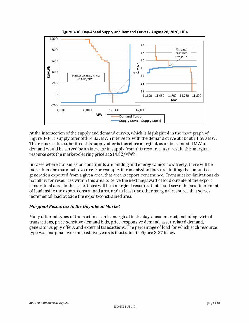
2020 Annual Markets Report page 125 ISO-NE PUBLIC
Figure 3-36: Day-Ahead Supply and Demand Curves - August 28, 2020, HE 6
At the intersection of the supply and demand curves, which is highlighted in the inset graph of Figure 3-36, a supply offer of $14.82/MWh intersects with the demand curve at about 11,690 MW. The resource that submitted this supply offer is therefore marginal, as an incremental MW of demand would be served by an increase in supply from this resource. As a result, this marginal resource sets the market-clearing price at $14.82/MWh.
In cases where transmission constraints are binding and energy cannot flow freely, there will be more than one marginal resource. For example, if transmission lines are limiting the amount of generation exported from a given area, that area is export-constrained. Transmission limitations do not allow for resources within this area to serve the next megawatt of load outside of the export constrained area. In this case, there will be a marginal resource that could serve the next increment of load inside the export-constrained area, and at least one other marginal resource that serves incremental load outside the export-constrained area.
Marginal Resources in the Day-ahead Market
Many different types of transactions can be marginal in the day-ahead market, including: virtual transactions, price-sensitive demand bids, price-responsive demand, asset-related demand, generator supply offers, and external transactions. The percentage of load for which each resource type was marginal over the past five years is illustrated in Figure 3-37 below.
-200
0
200
400
600
800
1,000
4,000 8,000 12,000 16,000
$/M
Wh
MW Demand CurveSupply Curve (Supply Stack)
Market Clearing Price: $14.82/MWh
12
13
14
15
16
17
18
11,600 11,650 11,700 11,750 11,800
$/M
Wh
MW
Marginal resource sets price
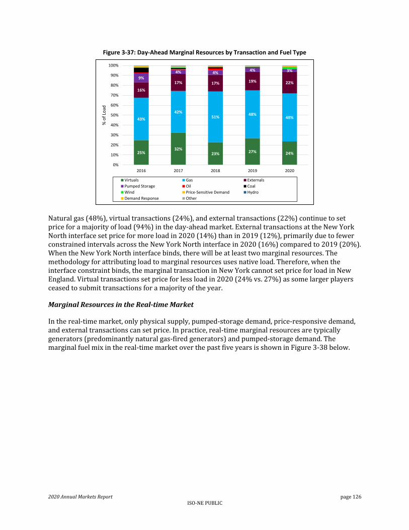
2020 Annual Markets Report page 126 ISO-NE PUBLIC
Figure 3-37: Day-Ahead Marginal Resources by Transaction and Fuel Type
Natural gas (48%), virtual transactions (24%), and external transactions (22%) continue to set price for a majority of load (94%) in the day-ahead market. External transactions at the New York North interface set price for more load in 2020 (14%) than in 2019 (12%), primarily due to fewer constrained intervals across the New York North interface in 2020 (16%) compared to 2019 (20%). When the New York North interface binds, there will be at least two marginal resources. The methodology for attributing load to marginal resources uses native load. Therefore, when the interface constraint binds, the marginal transaction in New York cannot set price for load in New England. Virtual transactions set price for less load in 2020 (24% vs. 27%) as some larger players ceased to submit transactions for a majority of the year.
Marginal Resources in the Real-time Market
In the real-time market, only physical supply, pumped-storage demand, price-responsive demand, and external transactions can set price. In practice, real-time marginal resources are typically generators (predominantly natural gas-fired generators) and pumped-storage demand. The marginal fuel mix in the real-time market over the past five years is shown in Figure 3-38 below.
25%32%
23% 27% 24%
43%
42%51%
48%48%
16%
17% 17% 19% 22%9%
4% 4%4% 3%
0%
10%
20%
30%
40%
50%
60%
70%
80%
90%
100%
2016 2017 2018 2019 2020
% o
f Lo
ad
Virtuals Gas Externals
Pumped Storage Oil Coal
Wind Price-Sensitive Demand Hydro
Demand Response Other
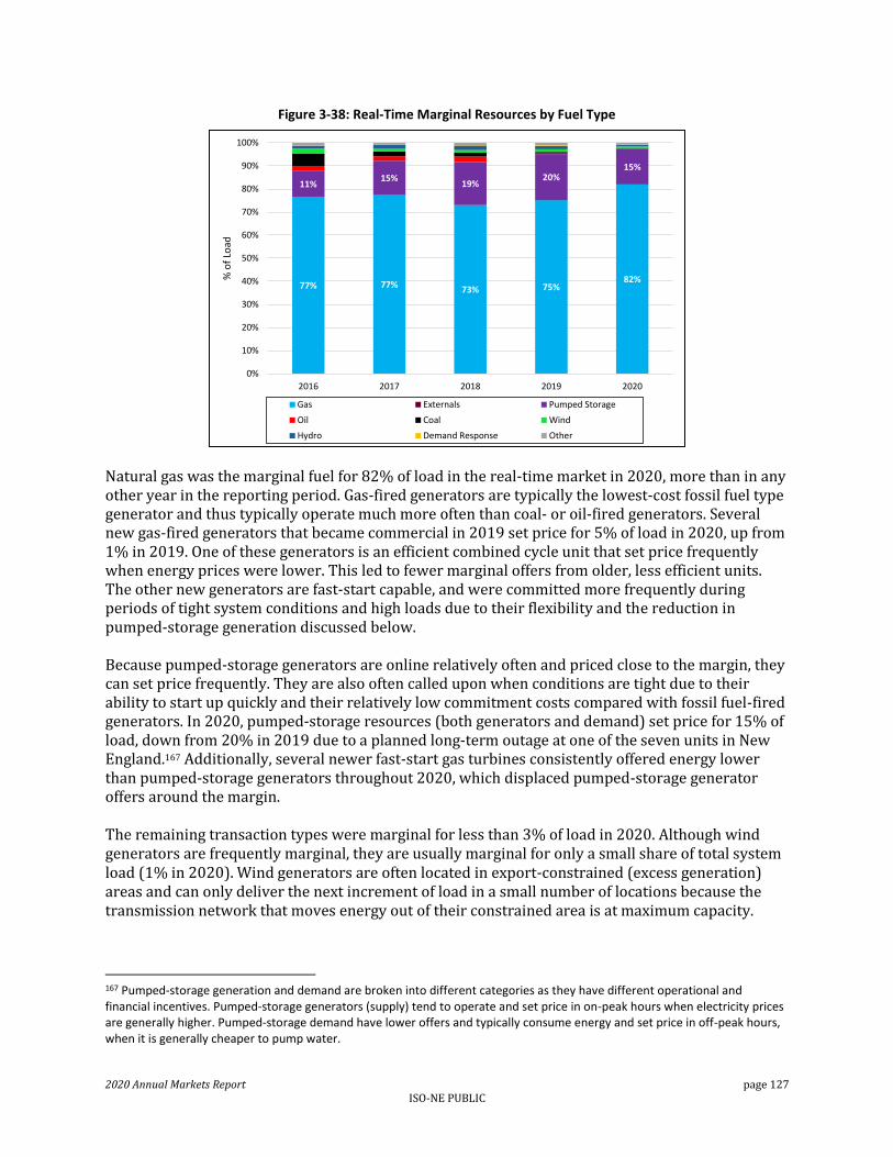
2020 Annual Markets Report page 127 ISO-NE PUBLIC
Figure 3-38: Real-Time Marginal Resources by Fuel Type
Natural gas was the marginal fuel for 82% of load in the real-time market in 2020, more than in any other year in the reporting period. Gas-fired generators are typically the lowest-cost fossil fuel type generator and thus typically operate much more often than coal- or oil-fired generators. Several new gas-fired generators that became commercial in 2019 set price for 5% of load in 2020, up from 1% in 2019. One of these generators is an efficient combined cycle unit that set price frequently when energy prices were lower. This led to fewer marginal offers from older, less efficient units. The other new generators are fast-start capable, and were committed more frequently during periods of tight system conditions and high loads due to their flexibility and the reduction in pumped-storage generation discussed below. Because pumped-storage generators are online relatively often and priced close to the margin, they can set price frequently. They are also often called upon when conditions are tight due to their ability to start up quickly and their relatively low commitment costs compared with fossil fuel-fired generators. In 2020, pumped-storage resources (both generators and demand) set price for 15% of load, down from 20% in 2019 due to a planned long-term outage at one of the seven units in New England.167 Additionally, several newer fast-start gas turbines consistently offered energy lower than pumped-storage generators throughout 2020, which displaced pumped-storage generator offers around the margin. The remaining transaction types were marginal for less than 3% of load in 2020. Although wind generators are frequently marginal, they are usually marginal for only a small share of total system load (1% in 2020). Wind generators are often located in export-constrained (excess generation) areas and can only deliver the next increment of load in a small number of locations because the transmission network that moves energy out of their constrained area is at maximum capacity.
167 Pumped-storage generation and demand are broken into different categories as they have different operational and financial incentives. Pumped-storage generators (supply) tend to operate and set price in on-peak hours when electricity prices are generally higher. Pumped-storage demand have lower offers and typically consume energy and set price in off-peak hours, when it is generally cheaper to pump water.
77% 77%73% 75%
82%
11%15%
19%20%
15%
0%
10%
20%
30%
40%
50%
60%
70%
80%
90%
100%
2016 2017 2018 2019 2020
% o
f Lo
ad
Gas Externals Pumped Storage
Oil Coal Wind
Hydro Demand Response Other

2020 Annual Markets Report page 128 ISO-NE PUBLIC
3.5 Net Commitment Period Compensation
This section provides an overview of Net Commitment Period Compensation (NCPC) payments. It covers payment types, reasons, and trends over the past five years.
Generators are eligible for NCPC or uplift payments when they are unable to recover their operating costs in the day-ahead or real-time energy markets. The uplift rules are designed to make generators that follow the ISO’s operating instructions no worse off financially than the generator’s next best alternative.168 Uplift is also paid to generators for “lost opportunities”, i.e. situations in which a generator foregoes opportunities for additional energy market revenue by following ISO instruction. This typically occurs when the market clearing software, or the ISO operators, restrict a generator’s output below its economically optimal level.
In 2020, uplift payments totaled $25.7 million, a decrease of $4.6 million (down by 15%) compared to 2019. Uplift payments remained relatively low, at 0.9%, when expressed as a percentage of total energy payments. Table 3-7 below details the continuing downward trend over the reporting horizon.
Table 3-7: Uplift Payments as a Percent of Energy Costs
Total uplift payments as a percent of energy costs were slightly higher in 2020 than in 2019 but remained below the five-year average of the reporting period.
3.5.1 Uplift Payment Categories
Generators that operate at the ISO’s instruction may be eligible for one of the following types of uplift depending on the reason for ISO commitment:
Economic/first-contingency NCPC169: o Out-of-merit NCPC: Payments provided to a generator committed in economic merit
order to satisfy system-wide load and reserves to cover the portion of as-offered costs not recovered through the LMP.
o External NCPC: Payments made to external and virtual transactions that relieve congestion at the external interfaces, and for external transactions that are unable to recover as-offered costs due to price forecast error.170
168 The terms “generators” or “generation” are used in this section in a broad sense; in practice, external transactions and pumped-storage demand also receive certain types of NCPC payments, but the vast majority of payments are made to generators.
169 A system’s first contingency (N-1) is the loss of the power system element (facility) with the largest impact on system reliability. A second contingency (N-1-1) takes place after a first contingency has occurred and is the loss of the facility that at that time has the largest impact on the system.
170 See Section 5.3 for further detail on external transaction uplift payments.
2016 2017 2018 2019 2020
Day-Ahead NCPC 1.1% 0.6% 0.4% 0.3% 0.3%
Real-Time NCPC 0.7% 0.5% 0.7% 0.4% 0.5%
Total NCPC as % Energy Costs 1.8% 1.2% 1.2% 0.7% 0.9%

2020 Annual Markets Report page 129 ISO-NE PUBLIC
o Dispatch lost opportunity cost NCPC (DLOC): Payments provided to a resource that is instructed by the ISO to run at levels below its economic dispatch point.
o Posturing NCPC: Payments provided to a resource that follows an ISO manual action that alters the resource’s output from its economically-optimal dispatch level in order to create additional reserves.
o Rapid-response pricing opportunity costs (RRP OC): Payments provided to a resource that is instructed by the ISO not to operate at its economic dispatch point when fast-start generators are setting the LMP.
Local second-contingency protection NCPC: Payments made to a generator committed to provide local operating reserve support in a transmission-constrained area to ensure local reliability needs.
Voltage reliability NCPC: Payments made to a generator that is dispatched to provide reactive power for voltage control or support.
Distribution reliability NCPC: Payments made to a generator committed to support local distribution networks, also known as special constraint resource or SCR payments.
Generator performance auditing NCPC: Payments made to a generator that is operating to satisfy the ISO’s performance auditing requirements.171
3.5.2 Uplift Payments for 2016 to 2020
Uplift payments decreased by $4.6 million (or by 15%) in 2020, from $30.3 million in 2019 to $25.7 million in 2020. This decrease follows the general downward trend of total uplift from 2016 through 2019, with the exception of higher uplift costs in 2018, which were largely due to a cold snap at the beginning of January. Local second-contingency protection payments explain most of the 2020 decrease, falling from $7.3 million in 2019 to $4.0 million in 2020. This is discussed further below.
Uplift Payments by Category
Over the past five years, most uplift payments have covered the operating costs of generators committed and dispatched in economic merit order (economic or first contingency), as shown in Figure 3-39 below. The inset table shows the percentage share of total uplift for each category by year.
171 Eligibility for payment under this uplift category includes: Performance audits of on-line and off-line reserves and for seasonal claimed capability audits initiated by the ISO rather than the participant, and dual-fuel testing.

2020 Annual Markets Report page 130 ISO-NE PUBLIC
Figure 3-39: Total Uplift Payments by Year and Category
Second contingency, distribution, and generator performance audit payments decreased in 2020, while economic and voltage payments increased by $0.2 and $0.1 million, respectively. Economic/first-contingency payments made up the bulk of uplift payments, totaling $19.6 million (or 76% of total payments). These payments were comparable to 2019, increasing slightly by $0.2 million and were $31 million (or 80%) lower than the high in 2018. Economic NCPC payments were only 0.6% of total energy payments, with a range of 0.5 to 0.9% over the reporting period.
Generator performance audit payments decreased by $1.2 million (or 57%) due to a reduction in audit commitments. Typically, ISO-initiated audits are conducted in the last quarter of the year, with some audits being scheduled in either September or January. In 2019, most audit commitments were made in November, averaging 11 MW per hour. In November 2020 audit commitments averaged just 5 MW per hour. Comparing year-over-year, the amount of audit commitments fell by 37% from 2019 to 2020.
Economic Uplift Sub-Categories
Out-of-merit and external uplift payments were the only sub-categories of uplift that increased in 2020. A breakdown of economic uplift by year and by sub-category is shown in Figure 3-40 below.
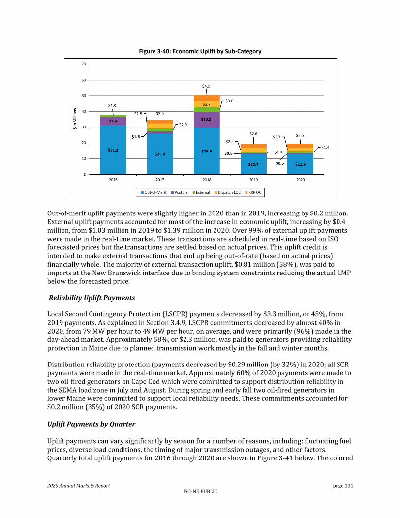
2020 Annual Markets Report page 131 ISO-NE PUBLIC
Figure 3-40: Economic Uplift by Sub-Category
Out-of-merit uplift payments were slightly higher in 2020 than in 2019, increasing by $0.2 million. External uplift payments accounted for most of the increase in economic uplift, increasing by $0.4 million, from $1.03 million in 2019 to $1.39 million in 2020. Over 99% of external uplift payments were made in the real-time market. These transactions are scheduled in real-time based on ISO forecasted prices but the transactions are settled based on actual prices. This uplift credit is intended to make external transactions that end up being out-of-rate (based on actual prices) financially whole. The majority of external transaction uplift, $0.81 million (58%), was paid to imports at the New Brunswick interface due to binding system constraints reducing the actual LMP below the forecasted price.
Reliability Uplift Payments
Local Second Contingency Protection (LSCPR) payments decreased by $3.3 million, or 45%, from 2019 payments. As explained in Section 3.4.9, LSCPR commitments decreased by almost 40% in 2020, from 79 MW per hour to 49 MW per hour, on average, and were primarily (96%) made in the day-ahead market. Approximately 58%, or $2.3 million, was paid to generators providing reliability protection in Maine due to planned transmission work mostly in the fall and winter months.
Distribution reliability protection (payments decreased by $0.29 million (by 32%) in 2020; all SCR payments were made in the real-time market. Approximately 60% of 2020 payments were made to two oil-fired generators on Cape Cod which were committed to support distribution reliability in the SEMA load zone in July and August. During spring and early fall two oil-fired generators in lower Maine were committed to support local reliability needs. These commitments accounted for $0.2 million (35%) of 2020 SCR payments. Uplift Payments by Quarter Uplift payments can vary significantly by season for a number of reasons, including: fluctuating fuel prices, diverse load conditions, the timing of major transmission outages, and other factors. Quarterly total uplift payments for 2016 through 2020 are shown in Figure 3-41 below. The colored

2020 Annual Markets Report page 132 ISO-NE PUBLIC
bars illustrate the quarterly uplift totals (Q1 is blue, Q2 is green, Q3 is red, and Q4 is yellow) and the black lines above the bars correspond to total annual uplift payments for that year.
Figure 3-41: Total Uplift Payments by Quarter
Similar to 2019, uplift payments by quarter continued to decrease and flatten out in 2020. The highest 2020 quarterly total uplift payments occurred in Q3 and Q4. Even though these two quarters were the highest of 2020, they were still consistent with or lower than Q3 and Q4 2019 payments. Uplift payments in Q3 2020 were $0.2 million higher than Q3 2019 however, Q4 2020 uplift payments were $2.7 million less than in Q4 2019. The increase in Q3 uplift payments was due to higher economic NCPC despite lower fuel prices. Significant nuclear refueling outages during this period resulted in less price-taking generation on the system. More expensive gas-fired generators were needed to meet system load and were eligible for NCPC payments, unlike nuclear generation. The majority of NCPC payments for local reliability commitments were in the latter half of year, like in 2019, but declined year over year. Between July and December, there were planned transmission outages in Maine and SEMA/Eastern Rhode Island that caused numerous day-ahead reliability commitments. Uplift by Fuel Type Total uplift payments by generator fuel type are shown in Figure 3-42 below.

2020 Annual Markets Report page 133 ISO-NE PUBLIC
Figure 3-42: Total Uplift Payments by Generator Fuel Type
Natural gas-fired and hydro generators received the majority (86%) of uplift payments because of their locational importance, both in the supply stack and geographically. These generators are often neither the least- nor most-costly generators, but are needed to ensure the reliable operation of the power system and are more economic to commit than very costly generators. Given some operational inflexibility (such as minimum run times), these generators may need to operate during hours when energy market prices do not allow them to fully recover their production costs. Pumped-storage generators continued to be the only fuel type that received posturing uplift payments ($0.5 million) in 2020. This is consistent with 2019 but differs from 2018 when oil-fired generators received uplift credits during a cold snap. In 2020 coal-fired generators received the smallest amount of uplift in the reporting period, 0.5% of total uplift payments or ($0.1 million). Compared to 2019 oil-fired generators received a lower share of uplift, 11% ($2.6 million) versus 14% ($4.0 million). Lastly, wind generators first started receiving relatively small amounts of uplift in 2017 and have received a steady 2% of total uplift payments (between $0.2 million and $1.1 million) a year since, mainly comprising dispatch lost opportunity cost payments, which are paid when resources are instructed to run at levels below their economic dispatch point.
3.6 Demand Resource Participation in the Energy and Capacity Markets
On June 1, 2018, the ISO implemented the Price-Responsive Demand (PRD) program to integrate demand response resources into the day-ahead and real-time energy markets in order to comply with FERC Order 745 (Demand-Response Compensation in Organized Wholesale Energy Markets).172 This program allows demand response resources to submit demand reduction offers into the day-ahead and real-time energy markets. With the program change, demand resources now are committed and dispatched in the energy market based on economics and are eligible to set price. Demand resources also provide operating reserves, in a manner similar to traditional
172 Prior to June 1, 2018, demand response resources participated in the ISO’s energy markets (1) as emergency resources activated during OP4 system conditions (i.e., a capacity deficiency) in the real-time market and (2) through the Transitional Price-Responsive Demand (TPRD) Program in the day-ahead market.
0
5
10
15
20
25
30
35
40
45
50
Co
al
Hyd
ro
Nat
ura
l Gas Oil
Win
d
Co
al
Hyd
ro
Nat
ura
l Gas Oil
Win
d
Co
al
Hyd
ro
Nat
ura
l Gas Oil
Win
d
Co
al
Hyd
ro
Nat
ura
l Gas Oil
Win
d
Co
al
Hyd
ro
Nat
ura
l Gas Oil
Win
d
2016 2017 2018 2019 2020
$ M
illio
ns

2020 Annual Markets Report page 134 ISO-NE PUBLIC
generators. Along with energy market integration, active demand resources are now treated similarly to other resources in the capacity market, having a must-offer obligation in the energy market for capacity with a capacity supply obligation (CSO).
In 2020, participation in the PRD program followed trends observed since the initial implementation in 2018:
Most PRD resources primarily served as capacity and operating reserve resources available for dispatch at very high offer prices:
o 83% of PRD capacity was offered at the energy market offer cap of $1,000/MWh in 2020; on average, 95% of offers have been priced above $200/MWh since the program’s implementation;
o Given offer prices, dispatch of these resources averaged just 3.2 MW in the day-ahead energy market and 4.3 MW in the real-time energy market in 2020; and,
o With low dispatch levels, energy market revenues totaled just $1 million for 2020. PRD resources represented a modest amount of overall capacity procured in the ISO’s
forward capacity market: o PRD resources provided approximately 438 MW of CSO on average in calendar year
2020, an increase of 39 MW over the prior calendar year; o PRD resources accounted for 1.2% of CSOs acquired in FCA 11; and, o Capacity payments provided to these resources totaled approximately $32 million in
2020.173
3.6.1 Energy Market Offers and Dispatch under PRD
Under the Price-Responsive Demand (PRD) program, over 500 MWs of demand response resources participate in the day-ahead and real-time energy markets, more than 100 MWs higher than pre-PRD active demand response participation levels. However, consistent with pre-PRD participation, demand resources continue to predominately function as capacity deficiency resources, providing a source of high-priced energy and 30-minute operating reserves in the real-time energy market.174 Figure 3-43 below indicates hourly demand reduction offers in the real-time energy market, by offer price category for segment energy offers.
173 This is a simple estimate that assumes all obligations received the auction clearing price.
174 Because these resources primarily function as a source of operating reserves and are dispatched at slightly higher levels (on average) in the real-time energy market, this section uses real-time offer and dispatch data to illustrate these resources’ participation in the ISO’s energy markets.

2020 Annual Markets Report page 135 ISO-NE PUBLIC
Figure 3-43: Demand Response Resource Offers in the Real-Time Energy Market
As indicated in the figure, most offers continue to be priced at the energy market offer cap of $1,000/MWh; 83% of offered capacity, on average, in 2020 and 75% in 2019. In most hours, only the lower tiers of offered capacity ($200/MWh or less) have a reasonable likelihood of being dispatched in the real-time energy market; these offers did not exceed 12% of offered demand reduction capacity in any hour of 2019 or 2020, and averaged just 5% of offered capacity.175
Given the pattern of offer prices for PRD, relatively small quantities are dispatched in the ISO’s energy markets. Figure 3-44 below illustrates the hourly dispatch of Demand Response Resources (DRRs) in the real-ahead energy market, relative to resources’ offered reductions and hourly energy prices.
175 Energy prices in the real-time market exceeded $200/MWh in just 0.16% of pricing intervals over the review period.
0
100
200
300
400
500
600
Jun
Jul
Au
g
Sep
Oct
No
v
Dec
Jan
Feb
Mar
Ap
r
May
Jun
Jul
Au
g
Sep
Oct
No
v
Dec
Jan
Feb
Mar
Ap
r
May
Jun
Jul
Au
g
Sep
Oct
No
v
Dec
2018 2019 2020
Off
ere
d E
ne
rgy
(MW
pe
r H
ou
r)
<$50 $50 to $100 $100 to $200 $200 to $500 $500 to $999 $1000
Offers at Low Prices
Offers at $1,000/MWh

2020 Annual Markets Report page 136 ISO-NE PUBLIC
Figure 3-44: Demand Response Resource Dispatch in the Real-Time Energy Market176
The maximum hourly quantity of demand response capacity dispatched in the real-time energy market was 107 MW in 2019 and 117 MW in 2020, representing approximately 32% of average offered demand reduction for those time periods. While demand resources were dispatched frequently in the real-time market – in 46% of hours in 2019 and 36% of hours in 2020 – the dispatch level was very small, averaging just 5.9 MW in 2019 and 4.3 MW in 2020.
As noted earlier, DRRs also provide a source of operating reserves in the real-time energy market. DRRs are considered fast-start capable, if those capabilities have previously been demonstrated. To be designated during the operating day as providing thirty-minute fast-start reserves, a DRR must offer certain operating constraints consistent with fast-start operation.177 While DRRs can provide ten-minute reserves, that service requires interval metering with granularity of one minute or less, to be able to provide either non-synchronized (TMNSR) or synchronized reserves (TMSR). In 2019, DRRs provided only 1.7 MW, on average, of ten-minute operating reserves, but provided substantially more in thirty-minute operating reserves (TMOR), averaging 223 MW per hour. In 2020, ten-minute reserve designations did not change substantially, decreasing to only 0.9 MW on average, but total thirty-minute operating reserves (TMOR) increased by 19% to 266 MW per hour, partially reflecting new capacity added in 2020.
3.6.2 NCPC and Energy Market Compensation under PRD
Demand Response Resources (DRRs) have received relatively modest energy market compensation during the review period. This results from low dispatch rates in the energy market and infrequent TMOR pricing in the real-time energy market. When dispatched, DRRs are eligible to receive uplift payments. NCPC provides additional compensation to resources when energy market revenues are
176 The right vertical axis (LMPs) has been truncated to improve the figure’s legibility. During the September 3, 2018 shortage event, real-time LMPs exceeded $500/MWh. The truncation obscures the magnitude of those prices, which reached as high as $2,677/MWh.
177 These operating constraints are: total start-up time (including notification time) of less than or equal to 30 minutes, minimum time between reductions and a minimum reduction time of less than or equal to 1 hour, and a “claim 30” (30-minute reserve capability) greater than 0.
-200
-100
0
100
200
300
400
500
-100
0
100
200
300
400
500
600
Jun
Jul
Au
g
Sep
Oct
No
v
Dec
Jan
Feb
Mar
Ap
r
May
Jun
Jul
Au
g
Sep
Oct
No
v
Dec
Jan
Feb
Mar
Ap
r
May
Jun
Jul
Au
g
Sep
Oct
No
v
Dec
2018 2019 2020
LMP
($
/MH
h)
MW
per
Ho
ur
RT Reduction Offers RT DRR Dispatch RT LMP

2020 Annual Markets Report page 137 ISO-NE PUBLIC
insufficient to cover as-offered operating costs in the day-ahead and real-time energy markets. Figure 3-45 indicates energy and NCPC payments by month.
Figure 3-45: Energy Market Payments to Demand Response Resources
As indicated in the figure, both NCPC payments and energy market payments have been relatively small, since the implementation of PRD in June 2018. Payments for NCPC represent just 17% of total energy market compensation for DRRs, and total energy payments for 2020 were only $1 million. (This compares to energy market payments of $3 billion for all resources during the full year.) Except for the elevated real-time energy market payments in August and September 2018 (resulting from a few hours of high reserve prices [August] and the capacity scarcity event [September]), day-ahead energy market payments have been the largest source of revenue for DRRs over the review period.178
3.6.3 Capacity Market Participation under PRD
For the Forward Capacity Market, DRRs had capacity supply obligations (CSOs) totaling approximately 438 MW in 2020, up by 39 MW (10%) compared to 2019.179 These resources are called “Active Demand Capacity Resources” (ADCR) for capacity market purposes. All active demand resources with capacity market obligations are required to offer “physically available” capacity into the day-ahead and real-time energy markets.180 Figure 3-46 indicates the CSO by participant for ADCRs.
178 Earlier versions of the graph did not include operating reserve revenues. Except for August and September 2018 (with operating reserve payments of approximately $200,000 per month), the inclusion of those revenues does not have a material impact on the previously-presented data.
179 The CSO estimate indicates the average capacity supply obligation for the calendar year.
180 The relationship between demand response resources (DRRs) and active demand capacity resources (ADCRs) is somewhat complicated. DRRs are mapped to ADCRs. More than one DRR can be mapped to an ADCR, which holds the capacity supply obligation. To satisfy the ADCR’s capacity supply obligation, DRRs mapped to an ADCR need to offer demand reductions into the energy market at an aggregate level consistent with the parent ADCR’s capacity supply obligation.
-0.2
0.0
0.2
0.4
0.6
0.8
1.0
1.2
1.4
1.6
Jun
Jul
Au
g
Sep
Oct
No
v
Dec
Jan
Feb
Mar
Ap
r
May
Jun
Jul
Au
g
Sep
Oct
No
v
Dec
Jan
Feb
Mar
Ap
r
May
Jun
Jul
Au
g
Sep
Oct
No
v
Dec
2018 2019 2020
Ene
rgy
Mar
ket
Pay
me
nts
($
mill
ion
s)
DA NCPC RT NCPC DA Energy RT Energy and Reserves
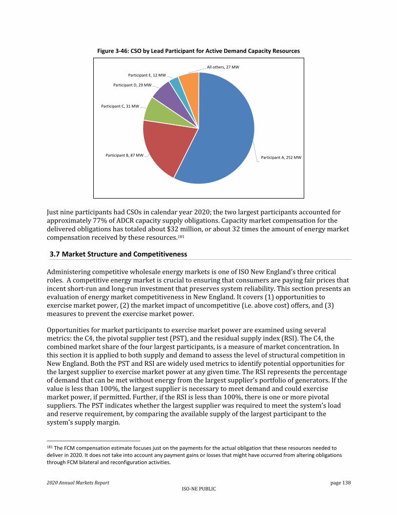
2020 Annual Markets Report page 138 ISO-NE PUBLIC
Figure 3-46: CSO by Lead Participant for Active Demand Capacity Resources
Just nine participants had CSOs in calendar year 2020; the two largest participants accounted for approximately 77% of ADCR capacity supply obligations. Capacity market compensation for the delivered obligations has totaled about $32 million, or about 32 times the amount of energy market compensation received by these resources.181
3.7 Market Structure and Competitiveness
Administering competitive wholesale energy markets is one of ISO New England’s three critical roles. A competitive energy market is crucial to ensuring that consumers are paying fair prices that incent short-run and long-run investment that preserves system reliability. This section presents an evaluation of energy market competitiveness in New England. It covers (1) opportunities to exercise market power, (2) the market impact of uncompetitive (i.e. above cost) offers, and (3) measures to prevent the exercise market power.
Opportunities for market participants to exercise market power are examined using several metrics: the C4, the pivotal supplier test (PST), and the residual supply index (RSI). The C4, the combined market share of the four largest participants, is a measure of market concentration. In this section it is applied to both supply and demand to assess the level of structural competition in New England. Both the PST and RSI are widely used metrics to identify potential opportunities for the largest supplier to exercise market power at any given time. The RSI represents the percentage of demand that can be met without energy from the largest supplier’s portfolio of generators. If the value is less than 100%, the largest supplier is necessary to meet demand and could exercise market power, if permitted. Further, if the RSI is less than 100%, there is one or more pivotal suppliers. The PST indicates whether the largest supplier was required to meet the system’s load and reserve requirement, by comparing the available supply of the largest participant to the system’s supply margin.
181 The FCM compensation estimate focuses just on the payments for the actual obligation that these resources needed to deliver in 2020. It does not take into account any payment gains or losses that might have occurred from altering obligations through FCM bilateral and reconfiguration activities.
Participant A, 252 MWParticipant B, 87 MW
Participant C, 31 MW
Participant D, 29 MW
Participant E, 12 MW
All others, 27 MW

2020 Annual Markets Report page 139 ISO-NE PUBLIC
The price-cost markup is presented to estimate the impact of uncompetitive offer behavior in the day-ahead energy market. To produce the price-cost markup, generator offers are replaced with estimates of each generator’s marginal cost and LMPs are re-simulated. The resulting value is an estimate of the LMP premium that is attributable to generators marking up their offers above marginal cost.
The IMM administers market power mitigation rules in the energy market to prevent potentially harmful effects of the exercise of market power. Mitigation is discussed at the end of this section.
3.7.1 C4 Concentration Ratio for Generation
This subsection analyzes supplier market concentration among the four largest firms controlling generation and scheduled import transactions in the real-time energy market. This measure, termed the “C4,” is useful in understanding the general trend in supply concentration as companies enter, exit, or consolidate control of supply serving the New England region over time.
The C4 is the simple sum of the percentages of system-wide market supply provided by the four largest firms in all hours of the year and accounts for affiliate relationships among suppliers. As shown in Figure 3-47 below, the C4 value of 41% for 2020, represents a small decline from 43% in 2019 and from the average for 2016–2019 (i.e., 44.5%).
Figure 3-47: Real-time System-wide Supply Shares of the Four Largest Firms
Note: The firms labeled “Supplier 1,” “Supplier 2” and so on are not necessarily the same companies across all years; these are generic labels for the top four firms during a given year.
The C4 values of the last five years range between 41-48%, indicating low levels of system-wide market concentration in New England, particularly because the market shares are not highly concentrated in any one company. In 2020, the total supply of generation and imports was about 63,700 GWh, of which about 25,800 (41%) came from the four largest suppliers. The red C4 trend line in Figure 3-47 shows no clear trend in the concentration ratio over the past five years. No one company maintains a dominant share of supply, and the split among the top four suppliers has remained stable.
43%48%
44% 43% 41%
0%
10%
20%
30%
40%
50%
60%
70%
80%
90%
100%
2016 2017 2018 2019 2020
Supplier 1 Supplier 2 Supplier 3
Supplier 4 Other Suppliers C4

2020 Annual Markets Report page 140 ISO-NE PUBLIC
3.7.2 C4 Concentration Ratio for Load
This section takes the same C4 metric discussed in the previous section and applies it to real-time load. The C4 for load measures the market concentration among the four largest load-serving entities (LSEs) in the real-time energy market. It also accounts for any affiliations among different LSEs. Figure 3-48 presents the results of the market share of the four largest LSEs along with the rest of market share during on-peak hours.
Figure 3-48: Real-time System-wide Demand Shares of the Four Largest Firms
Note: The firms labeled “LSE 1”, “LSE 2” and so on are not necessarily the same LSE across all years;
these are generic labels for the top four firms during a given year.
In 2020, the real-time load obligation (RTLO), or the amount of electricity purchased, was 59,820 GWh.182 Overall, the four largest LSEs served 60% (35,884 GWh) of total load, 2% higher than their share in 2019. The red C4 trend line in Figure 3-48 shows that the total load share of the four largest LSEs has steadily increased over the past five years. The increase is largely due to one participant obtaining a larger share of load. The C4 analyses presented here and in the previous section do not account for market participants with both load and generation positions. These firms generally have less incentive to exercise market power. Any spot market actions that would tend to raise prices for their generation would come at a cost to their load position. Any actions that would suppress prices for load would come at a cost to their generation position. The observed C4 values presented above indicate relatively low levels of system-wide market concentration, especially given the size of the New England market. The above figure shows that individual shares are not highly concentrated in any one company. Additionally, there is no evidence to suggest that LSEs exhibit any energy market bidding behavior that would suppress
182 Real-time load obligation is measured as all end-use wholesale load in the ISO New England region, along with all exports. The difference between this number and the real-time generation obligation should equate to energy losses.
50% 51% 53%58% 60%
0%
10%
20%
30%
40%
50%
60%
70%
80%
90%
100%
2016 2017 2018 2019 2020
LSE 1 LSE 2 LSE 3 LSE 4 Other LSEs C4

2020 Annual Markets Report page 141 ISO-NE PUBLIC
prices. Over 100% of demand clears in the day-ahead market and the aggregate demand curve is relatively price-insensitive around expected LMPs (see Section 3.4.5 on Demand Bidding).
3.7.3 Residual Supply Index and the Pivotal Supplier Test183
This section examines opportunities for participants to exercise market power in the real-time market using two metrics: the pivotal supplier test (PST) and the residual supply index (RSI). Both of these widely-used metrics identify instances when the largest supplier has market power.184 The RSI represents the amount of demand that the system can satisfy without the largest supplier’s available energy and reserves. If the value is less than 100, the largest supplier is needed to meet demand, and could exercise market power if permitted. Further, if the RSI is less than 100, there is one or more pivotal supplier. When the RSI exceeds 100, there is enough supply available to meet demand without any generation from the largest supplier. In this case, no individual supplier is pivotal and sufficient competition exists in the market.
The data used to calculate the RSI come from the ISO’s real-time market software (the Unit Dispatch System, or UDS). Based on these data, the RSI for an interval t is calculated as follows:
𝑅𝑆𝐼𝑡 =𝑇𝑜𝑡𝑎𝑙 𝐴𝑣𝑎𝑖𝑙𝑎𝑏𝑙𝑒 𝑆𝑢𝑝𝑝𝑙𝑦𝑡 − 𝐿𝑎𝑟𝑔𝑒𝑠𝑡 𝑆𝑢𝑝𝑝𝑙𝑖𝑒𝑟′𝑠 𝑆𝑢𝑝𝑝𝑙𝑦𝑡
𝐿𝑜𝑎𝑑𝑡 + 𝑅𝑒𝑠𝑒𝑟𝑣𝑒 𝑅𝑒𝑞𝑢𝑖𝑟𝑒𝑚𝑒𝑛𝑡𝑠𝑡
Pivotal suppliers are identified for every five-minute pricing interval by comparing the real-time supply margin185 to the sum of each participant’s total supply that is available within 30 minutes.186 When a participant’s available supply exceeds the supply margin, they are considered pivotal. The number of five-minute intervals with at least one pivotal supplier are divided by the total number of five-minute intervals in each quarter to obtain the percentage of intervals with pivotal suppliers.
The average RSI for all five-minute real-time pricing intervals and the percentage of five-minute intervals with pivotal suppliers are presented in Table 3-8 below.
Table 3-8: Residual Supply Index and Intervals with Pivotal Suppliers (Real-time)
Year % of Intervals With At
Least 1 Pivotal Supplier RSI
2016 48.4% 101.0
2017 55.7% 99.6
2018 30.7% 103.6
2019 14.7% 106.4
2020 16.6% 106.9
183 In this report, the RSI and pivotal supplier test are calculated using supply, load, and reserve requirement data from the ISO’s real-time market software. This differs from the calculation methodology of previous AMRs, which used the results and inputs of the real-time pivotal supplier test conducted by the mitigation software process.
184 When the RSI exceeds 100, there is enough supply available to meet demand without any generation from the largest supplier. In this case, no individual supplier is pivotal and sufficient competition exists in the market.
185 The real-time supply margin measures the amount of available supply on the system after load and the reserve requirement are satisfied. It accounts for ramp constraints and is equal to the Total30 reserve margin: 𝐺𝑒𝑛𝐸𝑛𝑒𝑟𝑔𝑦 + 𝐺𝑒𝑛𝑅𝑒𝑠𝑒𝑟𝑣𝑒𝑠 + [Net Interchange] -𝐷𝑒𝑚𝑎𝑛𝑑 - [𝑅𝑒𝑠𝑒𝑟𝑣𝑒 𝑅𝑒𝑞𝑢𝑖𝑟𝑒𝑚𝑒𝑛𝑡]
186 This is different from the pivotal supplier test performed by the mitigation software, which does not consider ramp constraints when calculating available supply for each participant. Additionally, the mitigation software determines pivotal suppliers at the hourly level.

2020 Annual Markets Report page 142 ISO-NE PUBLIC
There were significantly fewer five-minute intervals with pivotal suppliers in 2020 and 2019 than in 2016-2018. This indicates that during 2020 and 2019 suppliers faced relatively more competition compared to the three previous years. The reduction in the number of intervals with at least one pivotal supplier appears to be driven by two factors: 1) higher total 30-minute reserve margins in 2019 and 2020, and 2) the absence of significant changes in participant portfolios that would increase supply-side market concentration.
Higher supply margins are evident in the higher level of 30-minute operating reserves in 2020 and 2019 compared to the other years in the reporting period. In 2019, the average total 30-minute reserve surplus was 3,080 MW, up from 2,200-2,800 during 2016-2018. The increase was driven by additional off-line reserves from new generators and demand response resources. In 2020, the average total 30-minute reserve surplus was similar to the 2019 value, at 3,050 MW. Section 3.4.7 provides additional information on reserve margin trends. When reserve margins are higher, it is less likely that the available capacity of any one supplier is needed to satisfy load and reserve requirements.
Additionally, there were no significant changes in participant portfolios in 2019 and 2020. Market concentration and opportunities to exercise market power can increase if participants with large capacity volumes merge, but no notable activity occurred during the past two years. The C4 concentration ratio for generation, discussed in Section 3.7.1, was 41% in 2020, slightly lower than the 2019 and 2018 values due to decreased percentage shares across all four largest suppliers.
Duration curves that rank the average hourly RSI over each year in descending order are illustrated in Figure 3-49 below. The figure shows the percent of hours when the RSI was above or below 100 for each year. An RSI below 100 indicates the presence of at least one pivotal supplier.
Figure 3-49: System-wide Residual Supply Index Duration Curves
Like the pivotal supplier statistics, Figure 3-49 shows that there was greater availability of competitive supply in 2020 and 2019 than in any other year in the reporting period. The RSI was above 100 in 84% of real-time pricing intervals in 2020.
70
80
90
100
110
120
130
140
150
0% 20% 40% 60% 80% 100%
RSI
2020
2019
2018
2017
2016
Higher RSI in 68% of ranked observations in 2020 compared to 2019
No pivotal supplier in 84% of real-time intervals in 2020

2020 Annual Markets Report page 143 ISO-NE PUBLIC
3.7.4 Day-Ahead Price-Cost Markup187
In a perfectly competitive market, all market participants’ energy supply offers would equal their marginal costs.188 The energy component of the LMP would then be set by the supply offer or demand bid on the margin. In reality, participants can raise their supply offers above marginal costs. Though the IMM administers mitigation rules in the energy market to prevent the exercise of market power, participants are allowed to increase their offers by a certain threshold before mitigation is applied. The price-cost markup estimates the divergence of the observed market outcomes from the ideal scenario in which all energy supply is offered at marginal cost. The results provide insight on how uncompetitive offer behavior impacts the day-ahead energy market. Since market competition incentivizes participants to offer at marginal cost, the price-cost markup provides insight into market power and competitiveness. Uncompetitive offers priced above marginal cost can distort prices and impact generator commitment decisions, leading to inefficient market outcomes.
To calculate price-cost markup, the IMM simulated the day-ahead market clearing using two scenarios:
Scenario 1 is an offer case that uses actual day-ahead energy market supply offers submitted by market participants.
Scenario 2 is a marginal cost case that assumes all market participants offered at an estimate of their short-run marginal cost.189
The price-cost markup is then calculated as the percentage difference between the annual generation-weighted LMPs for the offer case and the marginal cost case simulations:
𝑃𝐶𝑀 =𝐿𝑀𝑃𝑂 − 𝐿𝑀𝑃𝑀𝐶
𝐿𝑀𝑃𝑂× 100
𝐿𝑀𝑃𝑂 is the annual generation-weighted LMP that results from actual generator offers, and
𝐿𝑀𝑃𝑀𝐶 is the annual generation-weighted LMP that would occur if generator offers were replaced with their respective marginal costs. A larger price-cost markup means that a larger component of the LMP is the result of inflated supply offers.
The annual day-ahead price-cost markup values from the simulation are shown in Table 3-9 below.
187 This section was titled “Lerner Index” in previous reports. The name was changed to better reflect the methodology behind the metric.
188 The IMM uses the PROBE, or “Portfolio Ownership and Bid Evaluation,” simulation model for this analysis. The software simulates the day-ahead LMP-based market clearing. See http://www.power-gem.com/PROBE.html. This is a more dynamic approach than calculating the difference between a static offer price and marginal cost. Rather, this approach re-runs the market optimization process with both as-offered and competitive (marginal cost) supply curves, and calculates the difference in the resulting LMPs.
189 The marginal costs estimates are based on underlying variable cost data and generator heat rate parameters used in the calculation of IMM reference levels. Reference levels are calculated pursuant to Appendix A to Market Rule 1 of the ISO tariff and are used in market power mitigation analyses to represent a competitive offer. Where a good estimate of marginal cost does not exist (for virtual transactions for example) the marginal cost is set equal to the supply offer. Some differences between estimated and actual marginal costs are to be expected.

2020 Annual Markets Report page 144 ISO-NE PUBLIC
Table 3-9: Day-Ahead Price-Cost Markup Percent
Year Price-Cost Markup
2016 8.2
2017 4.9
2018 4.9
2019 6.6
2020 7.6
The 2020 price-cost markup for the day-ahead energy market remained relatively low at 7.6%. This indicates that offers above marginal cost increased the generation-weighted day-ahead energy market price by approximately 7.6%. This result is similar to the 2019, and is consistent with normal year-to-year variation given modeling and estimation error.190 This indicates that competition among suppliers in the day-ahead market limited their ability to inflate LMPs by submitting offers above marginal cost.
This analysis also calculated price-cost markup values at an hourly level, and compared the peak load hour price-cost markup with the forecasted supply margin at peak. Comparing these attributes provides insight into whether participants take advantage of tight system conditions by exercising increased market power during those times. There was no meaningful correlation between the price-cost markup and the supply margin in 2020, indicating that the day-ahead market remained competitive even when the ISO expected supply margins to be low and market power was present.
3.8 Energy Market Mitigation
Mitigation rules, systems, and procedures are applied in the day-ahead and real-time energy markets to attenuate the impact of uncompetitive generator offers. The mitigation rules are intended to prevent market prices from being set above competitive levels and avoid the potentially harmful effects of market power. When a participant’s supply offer fails specific mitigation tests the offer is replaced with a competitive benchmark price known as the reference level. Generator reference levels are determined in consultation with the participant and are intended to reflect a competitive supply offer.191
This section provides an overview of the energy market mitigation tests and presents statistics on the occurrences of offer mitigation.
3.8.1 Types of Mitigation
There are eight types of energy market mitigation, each corresponding to a scenario where market power could be exercised. The two primary categories of mitigation are commitment scenarios and energy dispatch scenarios. Commitment mitigation pertains to generators that are started or kept
190 Note that the IMM’s estimates of marginal cost are an approximation of actual marginal costs, and the simulations used to calculate the price-cost markup are subject to modeling differences when compared to the market model the ISO runs for the day-ahead market.
191 There are three methodologies prescribed in Appendix A to Market Rule 1 for setting the reference level: (i) calculating the marginal cost of production, (ii) considering historical accepted supply offers, and (iii) using historical prices at the generator node. The IMM consults with the participant to determine the appropriate inputs to the marginal cost estimate. The highest value determined by these three methodologies is used to set the reference level except in certain circumstances.
2020 Annual Markets Report page 145 ISO-NE PUBLIC
on at the ISO’s request. Energy mitigation evaluates online generators that are dispatched by the market software or manual instructions.
Determining whether a participant’s supply offer must be mitigated involves up-to three tests depending on the applicable scenario: the structure, conduct, and impact tests.
Structure test. The market structure test evaluates the level of competition faced by a participant to determine whether they possess market power. A participant is deemed to have market power in any of three conditions. The first is when they are a pivotal supplier controlling resources needed to meet system-wide load and reserve requirements. The second condition is when their resource is in a constrained area of the system and has the ability to affect local area prices. And the third is when their resource is required to meet a specific reliability need such as voltage support; in this scenario the resource may be the only generator, or one of very few, capable of serving the need.
Conduct test. The conduct test checks whether the participant’s offer is above its competitive reference level by more than the allowed thresholds. The allowed threshold, expressed as a percentage or dollar amount, depends on the type of market structure test that applies in the scenario. The threshold values are tightest for scenarios where opportunities to exercise of market power are most prevalent.
Impact test. The market impact test gauges the degree to which the participant’s offer affects the energy LMP relative to an offer at its competitive reference level. The impact test applies to energy dispatch scenarios that require testing the incremental energy offers of online generators.
The participant’s offer must fail all the applicable tests in order for mitigation to occur. When a generator has been mitigated, all three components of the offer (i.e., start-up, no-load, and incremental energy) are replaced by the reference level values and mitigation remains in effect until the market power condition is no longer present.
An overview of energy market mitigation types and each of the tests applied for the scenario is provided in Table 3-10 below.192 Where a certain test is not applicable it is noted in the table with the text “n/a.” Note that the dollar and percentage thresholds specified for the conduct and impact tests are the values at which the participant’s offer is determined to fail the test.
192 Dual-fuel mitigation is excluded from the summary.

2020 Annual Markets Report page 146 ISO-NE PUBLIC
Table 3-10: Energy Market Mitigation Types
Mitigation type Structure test Conduct test threshold Impact test
General Threshold Energy (real-time only) Pivotal
Supplier
Minimum of $100/MWh and 300%
Minimum of $100/MWh and 200%
General Threshold Commitment (real-time only)
200% n/a
Constrained Area Energy Constrained Area
Minimum of $25/MWh and 50%
Minimum of $25/MWh and 50%
Constrained Area Commitment (real-time only)
25% n/a
Reliability Commitment Reliability 10% n/a
Start-Up and No-Load Fee n/a
200% n/a
Manual Dispatch Energy 10% n/a
Most mitigation types are applied in both the day-ahead and real-time markets, but the few that are only applied in real-time are indicated by the “(real-time only)” note below the mitigation type name in Table 3-10. Except for manual dispatch energy, the energy mitigation types involve all three tests. For commitment mitigation, only the structure and conduct tests apply since the impact on LMPs is not relevant to commitment events. Energy and commitment mitigation types also differ in terms of the supply offer components evaluated. For energy mitigation, only the incremental energy segments of the supply offer are relevant. In commitment tests, the aggregate cost of start-up, no-load, and incremental energy at minimum output (i.e., the commitment or “low load” cost) are evaluated over the commitment duration.
There is one additional mitigation type specific to dual-fuel generators not listed in Table 3-10 above. Dual-fuel mitigation occurs after-the-fact in cases where the supply offer indicated a generator would operate on a higher-cost fuel than it actually used (e.g., if offered as using oil, but the generator actually ran using natural gas). This mitigation will affect the amount of NCPC payments the generator is eligible to receive in the market settlements.
3.8.2 Mitigation Event Hours
This section summarizes energy market mitigation occurrences for 2016 - 2020. For these summaries, each hour that the submitted offer for an individual generator was mitigated in either the day-ahead or real-time energy market is counted as one observation (i.e., the tallies represent unit-hours of mitigation). For example, if a single generator offer was mitigated for five hours when committed in the day-ahead market, the mitigation count for this day will be five unit-hours. If a second generator offer was mitigated on the same day for three hours during real-time, the total would then be eight unit-hours.
In 2020, the total amount of mitigations increased relative to earlier periods. There were 1,270 unit-hours when some form of mitigation was applied. This is 40% higher than the 908 total unit-hours that occurred in 2019. As discussed below, increases in two types of mitigation resulted in the overall increase in mitigation hours for 2020, compared to earlier years: manual dispatch energy mitigation and dual-fuel mitigation.

2020 Annual Markets Report page 147 ISO-NE PUBLIC
To provide additional context, this section also summarizes the unit-hours that generators were evaluated for mitigation when they faced limited competition. These represent unit-hours when generators had potential market power. For example, a generator controlled by a “pivotal supplier” is considered to have potential market power.193 General threshold energy and general threshold commitment mitigation types apply to pivotal suppliers. Other instances of potential market power may occur in import-constrained areas (which may result in reduced competition), or when generators are committed to meet local reliability needs (such as local second contingency protection), or during periods of manual dispatch.
Figure 3-50 below indicates unit-hours of potential market power for the years 2016 to 2020.194
Figure 3-50: Unit-Hours with Potential Market Power Flagged
For all types of potential market power, instances of general threshold (i.e., pivotal supplier) and constrained area market power occur most frequently. All other instances of potential market power occur very infrequently. The significant decline in unit-hours for pivotal suppliers resulted from higher supply margins in later periods; the decline did not result from significant changes in participant portfolios.195 The frequency of constrained area market power follows the incidence of transmission congestion and import-constrained areas within New England. Since 2018, the frequency (in unit-hours) of constrained area instances has declined significantly; the higher instances of constrained areas prior to 2019 reflected transmission work in a number of load zones and a prolonged cold snap in 2018, both resulting in localized transmission congestion. The total unit-hours of on-line generation subject to mitigation rules is approximately 700,000 per year (denominator); given this, the portion of total unit-hours with potential market power has ranged
193 A participant is considered “pivotal” when energy market supply would be insufficient to meet demand, if that participant physically withheld its generation.
194 These data include all unit-hours of potential market power; during these hours, generators would be mitigated only when applicable conduct and impact test failures also occurred.
195 See Section 3.7.3 on the Residual Supply Index and the Pivotal Suppler Test.
9,871 27,594 33,437
211,568
281,191
135,194
44,307 33,484
0
50,000
100,000
150,000
200,000
250,000
300,000
350,000
2016 2017 2018 2019 2020
Un
it-H
ou
rs
Start-Up and No-Load Fee Reliability Constrained Area
General Threshold Manual Dispatch Energy Dual Fuel

2020 Annual Markets Report page 148 ISO-NE PUBLIC
from 42% in 2017 to 7% in 2020. The decline resulted from the large reductions in pivotal supplier (general threshold) and constrained area unit-hours.
Annual unit-hours of mitigations by type for each year between 2016 and 2020 are presented in Figure 3-51 below. Overall, mitigations occur relatively infrequently, compared to the instances of potential market power. As noted earlier, only 1,270 unit-hours of mitigation occurred in 2020, relative to the 43,500 unit-hours of potential market power (2.9%).
Figure 3-51: Mitigation Events, by Annual Period
The number of energy (i.e., non-commitment) mitigations doubled year-over-year in 2020 and also increased relative to earlier years. Energy mitigations increased to 316 unit-hours in 2020 from 156 unit-hours in 2019. This increase resulted from a 149 unit-hour increase in manual dispatch energy mitigations.196 This increase is explained by the offer behavior of two participants which had a substantial increases in energy offer mitigations for their generators, when manually dispatched. However, manual dispatch unit-hours in 2020 totaled approximately 1,900, resulting in a mitigation frequency of just 16%. Although general threshold (pivotal supplier) and constrained area mitigations have a high frequency of potential mitigation hours, both mitigation types occurred very infrequently in 2020 (with a combined total of just 11 unit-hours of mitigation); the low mitigation rate results primarily from the relatively high mitigation thresholds (i.e., conduct test and market impact test) that apply for these mitigation types. Dual-fuel mitigations represented the other significant increase in mitigation unit-hours. These mitigations increased from 26 unit-hours in 2019 to 335 unit-hours in 2020. They occurred more frequently in 2020 as a result of two participants using third-party software to adjust their energy market offers. The third-party software incorrectly stated the fuel type associated with energy market offers entered into the ISO’s data systems. This resulted in the need to mitigate generator offers after the fact, to ensure that uplift payments were not overstated.
196 Manual Dispatch Energy (MDE) Mitigation is applied to generators dispatched manually, out-of-merit by the ISO. When the system operator manually dispatches a generator out of merit for any reason, and the energy offer segment prices exceed the 110% mitigation threshold (relative to LMP), a generator will be mitigated for a period of time equal to (1) the duration of the dispatch period, (2) its return to its economic minimum, or (3) the generator’s offer price is equal to or less than the LMP.
1671
952704
672 514
335
154
175
156
305
0
500
1,000
1,500
2,000
2,500
2016 2017 2018 2019 2020
Un
it-H
ou
rs
General Threshold Energy General Threshold Commitment
Constrained Area Energy Constrained Area Commitment
Reliability Commitment Dual Fuel Resources
Start-Up and No-Load Fee Manual Dispatch Energy

2020 Annual Markets Report page 149 ISO-NE PUBLIC
Commitment mitigations declined by 15% in 2020, from 726 unit-hours in 2019 to 619 unit-hours in 2020. Reliability commitment mitigations represented the predominant commitment mitigation type, accounting for 83% (514 unit-hours) of commitment mitigation occurrences in 2020; reliability commitment mitigations declined by 24% in 2020. The reliability commitment mitigation hours (514) compare to a total of 3,200 reliability commitment hours, indicating a mitigation rate of 16%.
No general threshold commitment or constrained area commitment mitigations occurred in 2020; this lack of mitigation was primarily the result of relatively high conduct test thresholds.

2020 Annual Markets Report page 150 ISO-NE PUBLIC
Section 4 Virtual Transactions and Financial Transmission Rights
This section discusses trends in the use of two important financial instruments in the wholesale electricity markets: virtual transactions and financial transmission rights (FTRs).
The first type of financial instrument is a virtual transaction. Virtual transactions are financial bids and offers that allow participants to take a position on differences between day-ahead and real-time prices. Virtual transactions can improve market performance by helping converge day-ahead and real-time market prices. That is, virtual transactions can help ensure that the forward day-ahead market reflects expected spot prices in the real-time market, especially where systematic or predictable price differences may otherwise exist between them. However, virtual transactions are not costless – they are subject to NCPC charges that can often vary widely by day – and this cost can limit the ability of virtual transactions to perform this important market function.
In general, participants cleared similar levels of virtual transactions compared to the prior two years. However, cleared volumes remained higher than levels in 2016 as market rule changes created opportunities for virtual transactions to profit in New England’s day-ahead energy market and NCPC charges have fallen. Virtual transactions yielded higher profits in 2020 than in 2019, but profits remained below the levels seen from 2016 – 2018, despite lower NCPC charges in 2020.
The second type of financial instrument is a financial transmission right or “FTR”. These rights provide participants with physical generation or load in New England’s energy markets a way to manage the risks associated with transmission congestion in the day-ahead market. They also provide market participants a way to speculate on locational congestion differences in the day-ahead market. FTRs are purchased through ISO-administered auctions. In 2019, ISO-NE increased the number of opportunities it provides market participants to procure FTRs via auction when it implemented the Balance of Planning Period (BoPP) project on September 17, 2019.
As a whole, FTRs were unprofitable in 2020, marking the second straight year in which this was the case. This indicates that less congestion materialized in the day-ahead market than was expected by FTR market participants and reflected through FTR auction clearing prices. However, the magnitude of the losses decreased as total profitability for FTRs rose from negative $10.5 million in 2019 to negative $0.8 million in 2020. One factor for this this change in profitability between 2019 and 2020 was driven by the participants’ expectations for congestion over the New York – New England interface. Section 4.2 below discusses trends in FTRs.
4.1 Virtual Transactions
The first subsection (Section 4.1) provides an overview of virtual transactions and describes how they can benefit the wholesale energy market. However, the ability of virtual transactions to provide these benefits can be hindered by the transaction costs placed on them. One of these costs comes in the form of Net Commitment Period Compensation (NCPC) charges. This is the topic of subsection 4.1.2. The third subsection (4.1.3) examines virtual transaction profitability and how NCPC charges affected that profitability.
One of the primary benefits that virtual transactions can provide energy markets is to improve market efficiency, which, in this case, means achieving the commitments that are needed in the

2020 Annual Markets Report page 151 ISO-NE PUBLIC
real-time market at the lowest possible cost. Market participants can, by pursuing arbitrage opportunities or hedging, use virtual transactions to drive commitments made in the day-ahead market closer to the commitments that are needed in real-time. Improved commitment convergence is reflected through improved price convergence. The relationship between price convergence and virtual transaction volumes is examined in subsection 4.1.4. Lastly, subsection 4.1.5. summarizes some of the market rule changes implemented in New England’s energy markets over the last five years that likely had an impact on the use of virtual transactions.
Key Takeaways
In general, the volume of cleared virtual transactions increased from 2016 through 2018, but has remained steady since 2018. Cleared transactions rose from 475 MW per hour in 2016 to 990 MW per hour in 2018, on average. In 2020, cleared transactions averaged 975 MW per hour. Partly as a result of certain market rule changes, the increase in cleared virtual transactions has been more pronounced for virtual supply, which increased by 114% between 2016 and 2020. Cleared virtual demand increased 93% over the same period. The increase in cleared virtual transactions is also related to the relatively low real-time economic NCPC charge rates over most of the reporting period. From 2016 through 2019, this rate averaged about $0.84/MWh, and was particularly low in 2020, averaging around $0.46/MWh. While lower NCPC charges helped virtual supply remain profitable in 2020 (average net profit of $0.28/MWh), NCPC charges turned virtual demand profits on a gross basis into a net loss of $0.09/MWh, on average.
4.1.1 Virtual Transaction Overview
In the New England day-ahead energy market, participants submit virtual demand bids and virtual supply offers to profit from differences between day-ahead and real-time LMPs. One of the primary design goals of virtual transactions is that they can improve the day-ahead dispatch model to better reflect real-time conditions.197 Virtual demand bids and supply offers that clear in the day-ahead market (based on participants’ expectations of future real-time system conditions) can improve the generator commitments made in the day-ahead market. This is because the commitments that result from the day-ahead market clearing with virtual transactions will better reflect market participants’ combined expectations of real-time market conditions.
Virtual transactions that are profitable based on the price difference between the day-ahead and real-time markets generally improve price convergence. To see this, we can consider two examples. In the first example, day-ahead prices are systematically higher due to over-commitment in the day-ahead market. In this case, virtual suppliers (who are profitable when day-ahead prices are higher than real-time prices) can take advantage of the price difference by offering at lower prices than the physical generation, displacing some of it, while driving the day-ahead price downward toward the real-time price. In the second example, real-time prices are systematically higher due to under-commitment in the day-ahead market. In this case, virtual demand (which is profitable when real-time prices are higher than day-ahead prices) can take advantage of the price difference by bidding at higher prices than physical demand, resulting in more generation being committed in the day-ahead market, while driving the day-ahead price upward toward the real-time price.
197 Virtual transactions provide other market benefits than those discussed here. One of the most significant benefits is their ability to mitigate both buyer-side and seller-side market power through enhanced levels of competition. Additionally, virtual transactions increase the liquidity of the day-ahead market, which allows more participants to take forward positions in the energy market. Lastly, they can be used by participants as a way to manage/hedge the price risks associated with delivering or purchasing energy in the real-time energy market.

2020 Annual Markets Report page 152 ISO-NE PUBLIC
Virtual bids and offers can be submitted into the day-ahead market at any pricing location on the system during any hour. Virtual transactions clear in the day-ahead market like other demand bids and supply offers (see Section 3 for more information). The ISO settles virtual transactions based on the quantity of cleared virtual energy and the difference between the hourly day-ahead and real-time LMPs at the location. Cleared virtual supply offers make a “gross” profit if the day-ahead price is greater than the real-time price (sell high, buy back low), and cleared virtual demand bids make a gross profit if the day-ahead price is less than the real-time price (buy low, sell back high).
4.1.2 Virtual Transactions and NCPC
The ISO allocates the following NCPC charges to cleared virtual transactions:198
1. Real-time Economic NCPC: all cleared virtual transactions (supply and demand) are obligated to pay a per-MW charge to contribute towards the payment of real-time economic NCPC because they are considered real-time deviations.
2. Day-ahead Economic NCPC: virtual demand bids are also charged day-ahead economic NCPC based on their share of day-ahead load obligation. This charge is typically much smaller because the total day-ahead economic NCPC is divided among a much larger quantity of energy.
In general, the total profit after these two NCPC charges are levied will be referred to as “net” profit in this section. These NCPC charges effectively serve as “transaction costs” for virtual transactions, reducing a virtual transaction’s profit. Transaction costs can undermine price convergence when the expected magnitude in day-ahead to real-time price difference does not provide an adequate risk-adjusted return to offset the transaction costs. For example, if the expected spread (or gross profit) is $1/MW and the magnitude of NCPC charges (transaction cost) is uncertain, but may be greater than $1/MW, resulting in a net loss, then NCPC charges can discourage virtual participation, thus inhibiting price convergence. The IMM has recommended reviewing the allocation of NCPC charges to virtual transactions to ensure the charges are consistent with principles of cost causation and do not present a barrier to price convergence.
4.1.3 Virtual Transaction Profitability
Virtual transactions profit from spreads between day-ahead and real-time prices. However, NCPC charges can make virtual transactions that are profitable on a gross basis into unprofitable transactions on a net basis, limiting the ability of virtual transactions to close the spread between day-ahead and real-time prices.199 Figure 4-1 provides detail on the profitability of virtual transactions along with the impact of NCPC charges on profitability. The figure displays the average annual gross and net profit of virtual transactions since 2016. The bars are categorized by year and
198 Virtual transactions can also receive NCPC payments associated with congestion at the Non-CTS external interfaces. These payments are transfers between the participants causing the congestion and those relieving the congestion and are only applied to transactions that clear at these external interfaces. Because these NCPC charges do not have a broad market impact or apply to virtual transactions at most locations, they are not considered in much detail in this report. However, they are accounted for in the determination of net profitability for virtual transactions in Table 4-1 and Table 4-2. The NCPC credits (i.e., revenue) associated with relieving congestion at these external interfaces are also accounted for in the determination of net profitability in these two tables.
199 The NCPC charges to cleared virtual transactions are calculated after the market has cleared. However, participants most likely have a sense of what their expected exposure to NCPC charges is before submitting their virtual transactions. Relationships drawn in the analysis here presume participants are able to fairly accurately predict exposure to NCPC charges, which may not always be the case given the variability of such charges and the lack of information available to the participant in advance.

2020 Annual Markets Report page 153 ISO-NE PUBLIC
type with virtual demand shown in red and virtual supply shown in blue. The top of each bar represents gross profit, the bottom represents net profit, and the length of the bar represents the per-MW NCPC charge. The net profits consider real-time economic NCPC charges for both virtual demand and virtual supply as well as day-ahead economic NCPC charges for virtual demand. In addition, the dashed black line shows the percentage of hours during the year that virtual transactions were profitable on a gross basis, computed annually.200
Figure 4-1: Gross and Net Profits for Virtual Transactions
In 2020, virtual supply and virtual demand both had positive annual gross profits. While virtual supply was profitable, participants made an average gross profit of only $0.72/MW, the lowest gross profit over the last five years. Virtual demand gross profits increased significantly in 2020 ($1.56/MWh increase). Despite the increase, participants made an average gross profit of $0.36/MWh, the 2nd lowest profit level of the last five years. Virtual transactions were profitable on a gross basis in 53% of hours in 2020, down slightly from the prior year (56%).
NCPC charges for virtual transaction increased in 2020 compared to 2019 ($0.40/MWh to $0.46/MWh). However, NCPC charges during 2020 remained significantly below levels prior to 2019. From 2016 and 2018 NCPC charges averaged between $0.76/MWh and $1.25/MWh. In 2020, virtual supply remained profitable after NCPC charges were levied, making a net profit of $0.28/MWh, on average, while virtual demand made a net loss of $0.09/MWh.
Most Profitable Locations for Virtual Demand
The top 10 most profitable locations for virtual demand in 2020, after accounting for ISO-NE transaction charges and all relevant NCPC charges/credits, are shown in Table 4-1 below.201 These
200 The line is flat for observations in the same year because the value is computed as the number of hours that all virtual transactions together were profitable on a gross basis, as a percentage of total hours in the year.
201 The relevant NCPC charges/credits that are used in the calculation of net profitability for virtual transactions in Table 4-1 and Table 4-2 include not only the day-ahead and real-time economic NCPC charges discussed in detail in this section, but also the NCPC charges associated with causing congestion at non-CTS external interfaces, as well as the NCPC credits (i.e., revenue) associated with relieving congestion at these same interfaces.
50%
52%
54%
56%
58%
60%
($5)
($4)
($3)
($2)
($1)
$0
$1
$2
$3
$4
$5D
em
and
Sup
ply
De
man
d
Sup
ply
De
man
d
Sup
ply
De
man
d
Sup
ply
De
man
d
Sup
ply
2016 2017 2018 2019 2020
Pe
rce
nta
ge o
f H
ou
rs w
ith
Po
siti
ve G
ross
Pro
fit,
A
nn
ual
Le
vel O
bse
rvat
ion
s (L
ine
)
Vir
tual
Pro
fit
in $
/MW
h (
Bar
s)
Virtual Demand Profit Virtual Supply Profit Hours Virtuals Made Gross Profit
Gross Profit
Net Profit
NCPC Charge

2020 Annual Markets Report page 154 ISO-NE PUBLIC
locations are ranked by total net profit over the course of the year. The table also includes information about the volume of submitted and cleared MWs of virtual demand bids at each location, the profitability per MW, and the number of participants submitting virtual demand bids at each location.
Table 4-1: Top 10 Most Profitable Locations for Virtual Demand
Location Location Type
Submitted MWh
Cleared MWh
Gross Profit ($k)
Net Profit ($k)
Gross Profit Per MWh
Net Profit Per MWh
# of Participants
.Z.CONNECTICUT Load Zone 384,973 312,243 $316 $162 $1.01 $0.52 18
.Z.NEWHAMPSHIRE Load Zone 164,578 124,816 $139 $87 $1.11 $0.69 12
.Z.VERMONT Load Zone 108,253 83,444 $127 $84 $1.52 $1.00 8
LD.SHAWS_HL13.8 Load Node 12,471 9,743 $26 $20 $2.72 $2.09 4
UN.COSCOB 13.8CC10 Gen Node 11,229 3,732 $21 $19 $5.67 $5.08 2
LD.NORWALK 13.8 Load Node 9,932 2,494 $17 $16 $6.96 $6.50 2
LD.SOTHNGTN13.8 Load Node 13,973 10,045 $18 $16 $1.78 $1.55 6
UN.RISE 18.0RISE Gen Node 12,547 11,464 $16 $15 $1.39 $1.28 2
UN.RIDGEWOD13.8RIDG Gen Node 11,738 10,676 $16 $15 $1.49 $1.38 3
UN.OAKFIELD34.5OAKW Gen Node 34,321 12,173 $17 $15 $1.43 $1.20 10
The three most profitable locations for virtual demand in 2020 were all load zones (Connecticut, New Hampshire and Vermont). At these three locations, participants made $581,880 in gross profit and $332,276 in net profit. The New England West-East interface constraint contributed to the high net profit in two of these locations (.Z.CONNECTICUT AND .Z.VERMONT). This constraint is used to manage flows from western New England to eastern New England. This constraint bound in 2.4% of hours in the day-ahead market in 2020, but never bound in the real-time market.202 The New Hampshire-Maine Interface constraint contributed to higher net profits at the .Z.NEWHAMPSHIRE load zone. Together, these constraints resulted in lower prices on the western side of the constraints and higher prices on the eastern side in the day-ahead market, which tended not to materialize in real-time. Participants at these load zones benefitted from a difference in the congestion components at these locations between the day-ahead and real-time markets. While these locations had large profits, they also experienced much larger volumes of virtual transactions compared to the other 10 most profitable locations. Therefore, these locations experienced lower net profit per MWh (between $0.52/MWh and $1.00/MWh) compared to the other most profitable locations.
The other most profitable locations for virtual demand in 2020 were mostly nodes within the Connecticut or Rhode Island load zones. These locations often experienced negative congestion in the day-ahead market that did not occur as frequently in the real-time market. Excluding the load zones, the top 10 most profitable locations for virtual demand in 2020 were fairly lightly traded compared to the most profitable locations for virtual supply (see below) – both in terms of MW volumes and number of participants. Between two to ten different participants submitted virtual demand bids at these locations over the course of the year.
202 More information about this constraint can be found in Section 3.4.10.

2020 Annual Markets Report page 155 ISO-NE PUBLIC
While not shown in Table 4-1, some of the most active locations for virtual demand in 2020 (e.g., .H.INTERNAL_HUB, .Z.SEMASS, and .Z.NEMASSBOST) were some of the least profitable locations. In total, virtual demand transactions made a gross profit of $1.17 million, but a net loss of $0.35 million in 2020.
Most Profitable Locations for Virtual Supply
The top 10 most profitable locations for virtual supply in 2020, after accounting for transaction costs and NCPC charges/credits, are shown in Table 4-2 below. Again, these locations are ranked by total net profit.
Table 4-2: Top 10 Most Profitable Locations for Virtual Supply
Location Location Type
Submitted MWh
Cleared MWh
Gross Profit ($k)
Net Profit ($k)
Gross Profit Per MWh
Net Profit Per MWh
# of Participants
UN.BULL_HL 34.5BLHW Gen Node 193,163 128,394 $493 $430 $3.84 $3.35 16
UN.BULL_HL 34.5WEVW Gen Node 14,726 10,612 $250 $246 $23.57 $23.19 9
UN.ROLLINS 34.5ROLL Gen Node 104,024 78,779 $283 $246 $3.60 $3.12 14
UN.STETSON 34.5STE2 Gen Node 126,773 75,366 $215 $180 $2.85 $2.39 13
LD.KEENE_RD46 Load Node 117,275 58,654 $200 $170 $3.41 $2.91 10
UN.STETSON 34.5STET Gen Node 77,462 56,949 $169 $143 $2.96 $2.50 12
UN.BULL_HL 34.5HANW Gen Node 60,555 53,045 $155 $129 $2.93 $2.43 13
UN.OAKFIELD34.5OAKW Gen Node 267,638 182,612 $199 $115 $1.09 $0.63 17
UN.KIBBY 34.5KIBY Gen Node 91,511 46,924 $135 $109 $2.87 $2.33 16
UN.WASHNGTN34.5EPTD Gen Node 75,329 27,234 $102 $89 $3.74 $3.26 7
The most profitable locations for virtual supply in 2020 were mostly locations where wind power generators are interconnected. The one exception was a load node (LD.KEENE_RD46), which is behind an interface constraint that binds when wind or hydro power output is high. All wind generators are part of the set of resources known as DNE dispatchable generators (these are generators that operate under the Do Not Exceed (DNE) dispatch rules discussed below). These locations tend to be the most profitable given the opportunity virtual participants have to take advantage of the difference between day-ahead and real-time supply offers by DDGs. These locations were fairly competitive in 2020 with between 7 to 17 different participants offering virtual supply over the course of the year.
Participants made large profits at the second most profitable virtual supply location, UN.BULL_HL 34.5WEVW, despite low volumes compared to other wind generator nodes. Participants began clearing virtual supply offers at UN.BULL_HL 34.5WEVW beginning in October, around the same time a new generator interconnected at the node began testing for commercial operation. However, most of the profits at this location were made during the month of December, when the new generator began commercial operation. This led to increased congestion in this area of Maine. In total, virtual supply transactions made a gross profit of $3.84 million and a net profit of $1.39 million.
4.1.4 Price Convergence and Virtual Transaction Volumes
The ability of virtual transactions to help converge prices between the day-ahead and real-time markets is considered to be one of the primary benefits of virtual transactions in a two-settlement

2020 Annual Markets Report page 156 ISO-NE PUBLIC
system. The relationship between the volume of virtual transactions and the level of price convergence is shown in Figure 4-2 below. This figure presents two measures of price convergence:203
1) The mean absolute difference (in $/MWh) between the real-time and day-ahead Hub prices (blue line series).
2) The median absolute difference between real-time and day-ahead Hub prices as a percentage of the day-ahead Hub LMP (gray line series).
Figure 4-2: Virtual Transaction Volumes and Price Convergence
In 2020, the two measures of price convergence provide some evidence that the gap between day-ahead and real-time prices is narrowing. The average absolute price difference between the day-ahead and real-time Hub prices (blue line) was $5.48/MWh in 2020, the lowest level of the last five years. In the four prior years, this measure had fluctuated between $7.47/MWh (in 2019) and $12.58/MWh (in 2018). Price convergence also fell to its lowest level of the last five years as measured by the median absolute price difference between day-ahead and real-time Hub prices as a percent of the day-ahead Hub price (gray line). The median difference (as a percentage of the day-ahead Hub price) fell to 15.3% in 2020, down from the 16.7% observed in 2019. Section 3.3.5 discusses price convergence in more depth.
In general, the quantity of submitted virtual transactions has fallen over the last five years, while the level of cleared virtual transactions has increased. In 2020, participants submitted an average of 1,579 MWs of virtual transactions per hour. This represents a 25% decrease from the 2,095 MWs of virtual transactions that were submitted, on average, per hour in 2019, and a 56% decrease from the 3,549 MWs that were submitted, on average, per hour in 2016. One participant contributed significantly to the decrease in submitted virtual transactions. From 2016 through 2018, this participant submitted an average of 1,055 MWs per hour, but only submitted an average of 75 MW
203 For both of these metrics, the price difference is the absolute value of the day-ahead and real-time price difference. The absolute value is used because we are interested in virtual transactions’ potential impact on price convergence, including both positive and negative price differences. For the second metric, the price difference is divided by the day-ahead LMP to help normalize for systematic differences between prices in different years. The median is used to reduce the influence of outliers.
$5.48 /MWh
15.3%
(20)
(15)
(10)
(5)
0
5
10
15
20
25
(4,000)
(3,000)
(2,000)
(1,000)
0
1,000
2,000
3,000
4,000
5,000
2016 2017 2018 2019 2020
$/M
Wh
an
d %
Ae
rage
Ho
url
y V
olu
me
(M
W)
Bid Virtual Demand [left axis] Cleared Virtual Demand [left axis]Offered Virtual Supply [left axis] Cleared Virtual Supply [left axis]Avg. Absolute LMP Diff. ($/MWh) [right axis] Median LMP Diff. (% of DA LMP) [right axis]

2020 Annual Markets Report page 157 ISO-NE PUBLIC
per hour in 2020. However, cleared virtual transactions have generally increased over the last five years, rising from 475 MW per hour in 2016 to 975 MW per hour in 2020, on average. In fact, 62% of submitted virtual transaction MWs cleared in 2020, which was the highest level of the last five years. The increase in cleared virtual transactions has been particularly pronounced for virtual supply, which has increased by 114% (from 284 MW per hour to 607 MW per hour on average) in this five-year period.
4.1.5 The Impact of Market Rule Changes
Over the last five years, numerous market rule changes have been implemented in New England’s energy markets that have likely had an impact on, and created opportunities for, the use of virtual transactions. Among the relevant changes are: (i) modifications to the real-time commitment NCPC credit calculation, (ii) the implementation of Do-Not-Exceed (DNE) dispatch rules, and (iii) the implementation of Fast-Start Pricing (FSP). The period when each of these market rule changes took effect is depicted in Figure 4-3 below. This figure also shows the average hourly virtual transaction volumes by month over the period from 2016 through 2020, with virtual supply as positive values (in green) and virtual demand as negative values (in red). Each of these market rule changes is discussed in more detail below this figure.
Figure 4-3: Total Offered and Cleared Virtual Transactions by Quarter (Average Hourly MW)
Changes to NCPC rules
In February 2016 (gray shaded area), real-time economic NCPC payments made to generators with day-ahead commitments were eliminated, reducing the total pool of real-time economic NCPC paid. The average per MWh real-time NCPC charge was approximately $0.46 in 2020 versus $2.79 in 2015; the decrease in this average charge rate was driven mainly by the February 2016 rule change, other market rules changes discussed below, and lower energy costs.204 The lower real-time economic NCPC equated to reduced transaction costs for virtual transactions. This may partly
204 This subsection references 2015 since it was the last full calendar year without the changes to NCPC rules.
(4,000)
(3,000)
(2,000)
(1,000)
0
1,000
2,000
3,000
4,000
Q1 Q2 Q3 Q4 Q1 Q2 Q3 Q4 Q1 Q2 Q3 Q4 Q1 Q2 Q3 Q4 Q1 Q2 Q3 Q4
2016 2017 2018 2019 2020
Ave
rage
MW
pe
r H
ou
r
Cleared Virtual Demand Offered Virtual Demand
Cleared Virtual Supply Offered Virtual Supply
NCPC
DNE
FSP
DNE

2020 Annual Markets Report page 158 ISO-NE PUBLIC
explain the increase in cleared virtual transaction volumes after this rule change went into effect that can be seen in Figure 4-3.
Do-Not Exceed Dispatch Rules
Beginning in May 2016 (blue shaded area), certain wind and hydro generators became dispatchable under the Do Not Exceed (DNE) Dispatch rules. Under this change, DNE dispatchable generators (DDGs) can set price in the real-time energy market. DDGs tend to offer higher-priced energy in the day-ahead market due to a combination of factors, such as uncertainty about environmental and production conditions and terms under their power purchase agreements. Consequently, these generators often clear less day-ahead energy compared to their real-time production. In real-time, when there is more production certainty, these generators often reduce their offers and frequently set price.
This creates the opportunity for virtual supply to take advantage of the difference in day-ahead and real-time offer behavior. Since the implementation of DNE, virtual supply has frequently been marginal in the day-ahead energy market in geographic areas with DDGs. In the real-time energy market, DDGs have frequently been marginal in these same areas. The increase in cleared virtual supply after this rule change went in to effect is readily apparent in Figure 4-3.
Beginning in June 2019 (peach shaded area), ISO-NE implemented a requirement that all DDGs with Capacity Supply Obligations (CSOs) must offer the full amount of their expected hourly capability into the day-ahead energy market. This requirement reduced, but did not eliminate the opportunity for virtual transactions to participate in the day-ahead energy market in geographic areas with DDGs to the same extent as they did before this requirement went into effect. This is because this rule triggered more participation from intermittent power generators in the day-ahead market.
Fast-Start Pricing
In March 2017 (purple shaded area), new Fast-Start Pricing (FSP) rules went into effect. These changes more accurately reflect the cost of operating higher cost fast-start generators in the real-time market. The day-ahead market does not apply the FSP mechanics. Consequently, this change has the ability to increase real-time energy market prices relative to day-ahead prices, which may create more opportunities for virtual demand to converge prices. In the case of DNE and FSP, virtual transactions provide an important service to the market as they help converge day-ahead and real-time prices by reflecting expectations for real-time operating conditions in the day-ahead market. Virtual supply prevents higher-cost generators from being committed in the day-ahead market that would not actually be needed in real-time because of the lower-cost DDG generation that shows up in real-time. Virtual demand prevents under-commitment in the day-ahead market thereby preventing the need to commit fast-start generators in real-time.
4.2 Financial Transmission Rights
The first subsection (4.2.1) provides an overview of Financial Transmission Rights (FTRs) and gives details about how participants can purchase and sell FTRs in the various auctions that ISO-NE conducts. It also discusses how FTRs can be used both as a financial tool to hedge the risk of transmission congestion for physical supply or demand or as a completely speculative instrument. The supply and demand forces in the FTR market are then discussed. At the end of this subsection is an overview of the Balance of Planning Period (BoPP) project that ISO-NE implemented in September 2019. The next subsection 4.2.2 delves into the volume of FTRs purchased and considers

2020 Annual Markets Report page 159 ISO-NE PUBLIC
the impact that the COVID-19 pandemic may have had on the totals from 2020. This is followed by a subsection 4.2.3 that explores the funding of FTRs. The subsequent subsection (4.2.4) assesses the concentration of FTR ownership. The final subsection (4.2.5) examines the profitability of FTR holders in recent years, giving special attention to FTR paths that source from ISO-NE’s external node for trading across the New York – New England interface.
Key Takeaways
Over the last five years, there has been a steady decrease in the average MW-amount of FTRs held by participants; this value in 2020 (31,550 MW) is 13% less than the amount in 2016 (36,438 MW). The decrease in 2020 may be partly related to the economic shutdown that was intended to slow the spread of COVID-19, as there was a notable reduction in FTR purchases that occurred in the prompt-month auctions for April 2020 and May 2020. The expectation of lower loads during the shutdown may have led to an anticipation of lower congestion. In 2020, FTRs were fully funded, as they have been in each of the other years covered in this report. Meanwhile, the ownership of FTRs continued to be fairly highly concentrated in 2020 with around 60% of FTR MWs in both the on-peak and off-peak periods held by the top four participants. Additionally, 2020 was the second year in a row that FTR holders as a group were not profitable; together FTR holders lost $0.8 million in 2020. This comes after FTR holders made a loss of $10.5 million in 2019.
4.2.1 FTR Overview
FTRs provide participants with a way to hedge or speculate on transmission congestion in New England’s day-ahead energy market. Congestion occurs when the power flowing across a transmission element reaches the limit of what that element can reliably carry. When this happens, the power system must be re-dispatched away from the least-cost solution that existed in the absence of that limiting element. Re-dispatching resources incurs additional production costs on the power system because the most economic generation is not able to provide all the needed energy. The energy market reflects these additional costs through the congestion component of the LMP. FTRs provide participants with a mechanism to reduce their exposure to these additional costs. Transmission congestion is covered in more detail in Section 3.4.10.
Eligible bidders can obtain FTRs by participating in ISO-administered auctions for annual and monthly products. There are separate auctions for on-peak and off-peak hours.205 The FTRs awarded in the two annual auctions have a term of one year, while the FTRs awarded in one of the monthly auctions have a term of one month. FTRs can be purchased in all auctions, but can only be sold in the second annual auction or the monthly auctions as only FTRs that are owned (i.e., have been purchased) can be sold by participants (i.e., there is no short selling). Five important elements in a bid to purchase an FTR are summarized in Table 4-3 below.
205 On-peak hours are defined by the ISO as weekday, non-holiday hours ending 8-23. The remaining hours are off-peak hours.

2020 Annual Markets Report page 160 ISO-NE PUBLIC
Table 4-3: Elements of an FTR Bid
Once FTRs are awarded, target allocations for each FTR are calculated on an hourly basis as appropriate based on the term (e.g., November 2020) and period (i.e., on-peak or off-peak) of the FTR. Target allocations are calculated by multiplying the MW amount of the FTR by the difference in the day-ahead congestion components of the FTR’s sink and source locations. Positive target allocations occur when the congestion component of the sink location is greater than the congestion component of the source location in the day-ahead energy market. Positive target allocations represent revenue to FTR holders. Negative target allocations, which occur when the congestion component of the sink location is less than the congestion component of the source location in the day-ahead energy market, represent a charge to FTR holders. Payments to FTR holders with positive target allocations come from day-ahead and real-time congestion revenue and from FTR holders with negative target allocations.
Hedging vs. Speculating
To understand how an FTR could be used to hedge congestion risk, we can consider a simple example of a load-serving entity (LSE) located in an import-constrained area (i.e., an area prone to positive congestion) that has entered into an annual contract to buy energy at the day-ahead Hub price. This contract locks-in the energy component of the price that the LSE must pay, but not the congestion component. Absent ownership of an FTR, the LSE still bears the congestion cost risk associated with serving load in an area prone to positive congestion. The LSE can lock-in the congestion component as well by participating in the annual on- and off-peak FTR auctions. Purchasing an FTR from the Hub to the zone where it serves energy in both these auctions entitles the LSE to the difference in the congestion components at these locations over the course of the year. The positive target allocations that accrue to the FTRs that the LSE holds offset the day-ahead congestion costs that the LSE incurs in the zone where it serves load. The cost required to hedge this congestion risk is the price the LSE paid to purchase these FTRs.
FTRs can also be purchased as a completely speculative instrument. For example, a market participant that has no load or generation position may want to purchase an FTR solely because it expects a certain amount of positive target allocations to accrue along a specific path.206 This transaction would be profitable if the participant is able to purchase the FTR at a cost that is less than the revenue realized from holding the FTR. Such activity is not without risk, as expected
206 This example is for a prevailing flow FTR, which is an FTR whose path is defined in the direction that congestion is expected to occur based on FTR auction clearing prices. The holder of a prevailing flow FTR pays to acquire that FTR and then expects to receive positive target allocations as congestion occurs in the day-ahead energy market. Alternatively, a speculator could acquire a counterflow FTR. An FTR purchased at a negative price in an auction is called a counterflow FTR because its path is defined in the opposite direction that congestion is expected to occur based on the FTR auction clearing prices. The auction pays the counterflow FTR holder to take on this counterflow position, and this position will be profitable to the counterflow FTR holder if the total negative target allocations for this FTR are less than this payment from the auction.
Element Description
Path FTRs are defined between two points (locations) on the electrical system: 1) the point
of withdrawal or the “sink” and 2) the point of injection or the “source”
Price The $/MW value the participant is willing to pay to acquire the FTR
MW-amount The size of the FTR (in MWs) the participant is willing to buy
Term The monthly or annual period to which the FTR applies (e.g., November 2020)
Period The hours in which the FTR applies (i.e., on-peak or off-peak)

2020 Annual Markets Report page 161 ISO-NE PUBLIC
patterns of congestion may not actually appear in the day-ahead market. In such cases, FTRs can quickly change from being a financial benefit to a financial obligation that requires payment. This sort of trading is considered speculative because it is an attempt to profit by engaging in a risky financial transaction that is not tied to any physical position in the ISO-NE marketplace. Speculative trading is permitted in FTR auctions because of the liquidity and competition it provides.
Supply and Demand
The demand for FTRs is primarily driven by participants’ expectations of congestion in the day-ahead market. If participants expect less day-ahead congestion than in prior years, their need to purchase FTRs to hedge against this congestion may decrease. The volume of FTR purchases is particularly dependent on the variability of participants’ expectations of congestion. For example, if all participants have the same expectation for congestion in a certain year, the set of FTR paths that they bid on is likely to be limited, which would result in fewer FTRs being purchased. Additionally, participants may be unwilling to take counterflow FTR positions if they hold comparable outlooks.207 On the other hand, if participants have a diverse range of expectations for congestion, the set of FTR paths that they bid on is likely to be larger, and more participants may be willing to take counterflow positions.
The supply side of the FTR market is predominantly dependent on the physical capability of the transmission system. The amount of FTRs awarded by the ISO in each auction depends on a market feasibility test that ensures that the awarded set of FTRs respects the transmission system’s limits under normal and post-contingent states. This test is performed in order to increase the likelihood of revenue adequacy, which means that the FTRs are fully funded; in other words, that there is sufficient congestion revenue collected in the energy market and from FTR holders with negative target allocations to fully compensate all FTR holders with positive target allocations. The funding of FTRs is looked at more closely later in this section.
Balance of Planning Period Project (BoPP)
On September 17, 2019, ISO-NE implemented the Balance of Planning Period (BoPP) project for FTRs. This project increased the number of opportunities that market participants have to reconfigure their monthly FTR positions following the two annual auctions. Prior to the implementation of this project, market participants could only purchase or sell FTRs for a specific month in the auction that occurred during the month prior to that effective month. For example, under the old design, if a market participant wanted to buy FTRs that would be effective for December 2020, it had to wait until the monthly auction that took place in November 2020. Under the BoPP design, ISO-NE now administers monthly FTR auctions for not just the next month (now called the prompt-month auction), but also for all the other months remaining in the calendar year (called the out-month auctions). This means that a participant who wants to buy December 2020 FTRs no longer has to wait until November 2020; it can purchase these FTRs in any of the out-month auctions that take place earlier in the year.
Importantly, the out-month auctions do not make more network capacity available than was made available in the second annual auction (in contrast to the prompt-month auctions, which do make additional capacity available). One quarter of the transmission system capability is made available
207 The purchase of counterflow FTRs is important because it impacts the supply of FTR MWs. This is because every MW purchased on a counterflow path (say from B to A) allows participants to buy an additional MW of the prevailing flow path (in this case, A to B).

2020 Annual Markets Report page 162 ISO-NE PUBLIC
in the first round of the annual auction. An additional quarter of the transmission system capability is made available in the second round of the annual auction, meaning that 50% of the network capability is available to be sold in the two annual auctions. The prompt-month auctions make available an additional 45% of the network capability, meaning that 95% of the network capability is available to be sold by the time the effective month arrives. While the out-month auctions do not make available any additional network capability beyond that which was made available in the second round of the annual auction, FTRs can still be purchased in these auctions. Additional FTR purchases could occur on paths that were not completely subscribed in the second annual auction, as the result of counterflow FTR purchases, or as the result of FTR sales.
4.2.2 FTR Market Volume
Fewer FTRs (by MWs) were in effect per hour, on average, in 2020 than in 2019, continuing a trend of steady decreases in FTR MWs that has occurred over the last five years. This trend can be seen in Figure 4-4, which shows the average MW volume of FTRs that were in effect each hour by year between 2016 and 2020 as black diamonds.208 This figure also shows the average hourly MW volume of FTRs purchased and sold by auction type (i.e., annual, prompt-month, or out-month) during each year.
Figure 4-4: Average FTR MWs in Effect per Hour by Year
Market participants had an average of 31,550 MWs of FTRs in effect per hour in 2020. This represents a modest 1% decrease from the average amount of FTRs in effect in 2019 (31,981 MW) and a 13% decrease from the average amount in effect in 2016 (36,438 MW). FTR MW purchases in the annual auctions increased by 4% between 2019 and 2020, rising from an average of 18,488 MWs per hour to 19,138 MWs per hour. However, prompt-month FTR purchases fell considerably from their 2019 level, dropping from an average of 13,746 MWs per hour to 10,644 MWs per hour – a decrease of 23%. It could be the case that some of the purchases that would have happened in the prompt-month auctions prior to the implementation of BoPP are now taking place in the earlier
208 The averages are hourly-weighted MW volumes. This weighting accounts for the fact that there are more off-peak hours than on-peak hours in a year. The hourly-weighted average MW volume of FTRs in effect each year represents the hourly-weighted average MW volume of FTRs purchased less the hourly-weighted average MW volume of FTRs sold.
(5,000)
0
5,000
10,000
15,000
20,000
25,000
30,000
35,000
40,000
2016 2017 2018 2019 2020
Ave
rage
MW
pe
r H
ou
r
Annual Purchased MW Annual Sold MWPrompt Purchased MW Prompt Sold MWOut-month Purchased MW Out-month Sold MWAverage MW in Effect
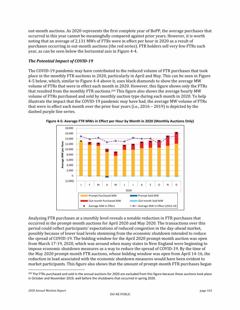
2020 Annual Markets Report page 163 ISO-NE PUBLIC
out-month auctions. As 2020 represents the first complete year of BoPP, the average purchases that occurred in this year cannot be meaningfully compared against prior years. However, it is worth noting that an average of 2,131 MWs of FTRs were in effect per hour in 2020 as a result of purchases occurring in out-month auctions (the red series). FTR holders sell very few FTRs each year, as can be seen below the horizontal axis in Figure 4-4.
The Potential Impact of COVID-19
The COVID-19 pandemic may have contributed to the reduced volume of FTR purchases that took place in the monthly FTR auctions in 2020, particularly in April and May. This can be seen in Figure 4-5 below, which, similar to Figure 4-4 above it, uses black diamonds to show the average MW volume of FTRs that were in effect each month in 2020. However, this figure shows only the FTRs that resulted from the monthly FTR auctions.209 This figure also shows the average hourly MW volume of FTRs purchased and sold by monthly auction type during each month in 2020. To help illustrate the impact that the COVID-19 pandemic may have had, the average MW volume of FTRs that were in effect each month over the prior four years (i.e., 2016 – 2019) is depicted by the dashed purple line series.
Figure 4-5: Average FTR MWs in Effect per Hour by Month in 2020 (Monthly Auctions Only)
Analyzing FTR purchases at a monthly level reveals a notable reduction in FTR purchases that occurred in the prompt-month auctions for April 2020 and May 2020. The transactions over this period could reflect participants’ expectations of reduced congestion in the day-ahead market, possibly because of lower load levels stemming from the economic shutdown intended to reduce the spread of COVID-19. The bidding window for the April 2020 prompt-month auction was open from March 17-19, 2020, which was around when many states in New England were beginning to impose economic shutdown measures as a way to reduce the spread of COVID-19. By the time of the May 2020 prompt-month FTR auctions, whose bidding window was open from April 14-16, the reduction in load associated with the economic shutdown measures would have been evident to market participants. This figure also shows that the amount of prompt-month FTR purchases began
209 The FTRs purchased and sold in the annual auctions for 2020 are excluded from this figure because these auctions took place in October and November 2019, well before the shutdowns that occurred in spring 2020.
(2,000)
0
2,000
4,000
6,000
8,000
10,000
12,000
14,000
16,000
18,000
J F M A M J J A S O N D
2020
Ave
rage
MW
pe
r H
ou
r
Prompt Purchased MW Prompt Sold MW
Out-month Purchased MW Out-month Sold MW
Average MW in Effect Average MW in Effect (2016-19)

2020 Annual Markets Report page 164 ISO-NE PUBLIC
to increase in every month after May 2020 and that the average MW volume of FTRs that were in effect returned to historically observed levels at the end of the year. The reduction in load associated with the COVID-19 pandemic is discussed in more detail in Section 3.4.4.
4.2.3 FTR Funding
The congestion revenue fund has ended with a surplus in each of the last five years as can be seen by the blue line in Figure 4-6 below. This figure also shows the different components that affect the congestion revenue fund balance, and provides the percent of positive target allocations that were paid each year (indicated by number above each stacked column).210 A value of 100% indicates that the FTRs were fully funded that year.
Figure 4-6: Congestion Revenue Fund Components and Year-End Balance by Year
In 2020, the congestion revenue fund had a year-end balance of $6.1 million.211 This represents a 30% decrease from the fund balance of $8.7 million in 2019. Day-ahead congestion revenue in 2020 ($29.7 million) was almost perfectly offset by the amount of positive target allocations ($29.5 million). As the real-time congestion revenue in 2020 was only -$0.6 million, the primary reason for the fund surplus in 2020 was the negative target allocations, which amounted to $6.6 million. This represents a 101% increase from the level observed in 2019 ($3.3 million). One transmission constraint from the day-ahead market that led to a significant amount of negative target allocations in 2020 was the New England West-East interface constraint (more information about what led this constraint to bind can be found in Section 3.4.10).
FTRs have been fully funded for each of the last five years as indicated by the labels above the yearly bars in Figure 4-6. As FTR settlement occurs on a monthly basis, there were several months in 2020 in which FTRs were not fully-funded – specifically February, May, and August. However,
210 The congestion revenue fund balance is equal to the sum of the congestion revenue from the day-ahead and real-time energy markets plus the revenue from negative target allocations less the revenue to positive target allocations. The congestion revenue fund is also discussed in Section 3.4.10.
211 The $6.1 million total for 2020 represents the amount in the congestion revenue fund after fully funding any FTRs that had been underfunded during any month in the year.
100%100%
100%
100% 100%
(80)
(60)
(40)
(20)
0
20
40
60
80
100
2016 2017 2018 2019 2020
Co
nge
stio
n R
eve
nu
e F
un
d C
om
po
ne
nts
($
mill
ion
s)
Day-Ahead Congestion Revenue Negative Allocations
Positive Allocations Real-time Congestion Revenue
% - Percent of Positive Allocations Paid Congestion Revenue Fund Year-End

2020 Annual Markets Report page 165 ISO-NE PUBLIC
there was sufficient revenue in the fund at the end of the year to make these FTRs whole. The remaining year-end fund surplus was then allocated to entities that paid congestion costs during the year in a proportion to the amount of congestion costs they paid.212
4.2.4 FTR Market Concentration
The concentration of ownership of FTRs among market participants in 2020 was similar to prior years. The average amount of FTRs held per hour by the top four participants with the most MW each year is shown in Figure 4-7 below. Also included in this figure is the number of different participants that held FTRs each year (indicated by the number above each stacked column).This figure provides information for both the on-peak and off-peak periods.
Figure 4-7: Average FTR MWs Held by Top Four FTR Holders per Hour by Year and Period
Note: The firms labeled “Participant 1,” “Participant 2” and so on are not necessarily the same
companies across all years; these are generic labels for the top four firms during a given year.
In 2020, the percentage of on-peak FTR MWs held by the top four participants was 58%. This ratio is often referred to as the C4. The off-peak concentration ratio of the top four FTR holders in 2020 was similar to the on-peak; the top four participants held 59% of the off-peak FTR MWs. The concentration ratio of the top four FTR holders has trended downward slightly over the last two years. The off-peak period C4 reached a maximum of 70% in 2017, while the on-peak period C4 reached its highest value of 67% in 2018. The total number of unique FTR holders has stayed relatively steady over the reporting period, ranging between 38 to 45 different participants.
4.2.5 FTR Profitability
As a group, FTR holders were not profitable in 2020.213 Profit in the FTR market is measured as the sum of the positive target allocations and the revenue from FTR sales, minus negative target
212 See Section III.5.2.6 of Market Rule 1 for more information.
213 While FTR holders as a group were unprofitable in 2020, some specific market participants did earn a profit.
39 4038 39
40 3945 45 39 39
0
5,000
10,000
15,000
20,000
25,000
30,000
35,000
40,000
45,000
Off-peakOn-peakOff-peakOn-peakOff-peakOn-peakOff-peakOn-peakOff-peakOn-peak
2016 2017 2018 2019 2020
Ave
rage
MW
pe
r H
ou
r
Participant 1 Participant 2 Participant 3
Participant 4 Other Participants # - Number of Participants

2020 Annual Markets Report page 166 ISO-NE PUBLIC
allocations and the cost of FTR purchases. Each of these components as well as total profit (purple line) can be seen in Figure 4-8 below.
Figure 4-8: FTR Costs, Revenues, and Profits
In 2020, the total profit from FTRs was -$0.8 million (purple line), which is an increase of $9.7 million from 2019, when total FTR profit was -$10.5 million. Two primary factors led to the increase in FTR profitability in 2020:
1. Positive target allocations increased. Payments to FTR holders with positive target allocations increased by $2.0 million in 2020 ($29.5 million) relative to 2019 ($27.5 million). Positive target allocations in 2019 were at their lowest level of the last five years.
2. FTR purchase costs decreased. Participants spent $11.3 million less to procure FTRs in 2020 than they did in 2019. The decrease in purchase costs was particularly notable in the non-annual auctions, where participants decreased their FTR expenditures by 47% between 2019 ($16.4 million) and 2020 ($8.7 million).
Most Profitable FTR Paths
Significant investment in transmission infrastructure over the past ten years, targeted primarily at import-constrained areas, has reduced the amount of positive congestion in the New England footprint. However, the growth in wind power and other factors has led to more export-constrained areas, which, in turn, has led to more negative congestion. This type of congestion can be hedged by procuring FTRs that source from within the area experiencing the negative congestion and that sink in a location outside the constrained area (the Hub is frequently used by participants). Many of the most profitable FTR paths in 2020 were this type of path. This is reflected in Table 4-4 below, which provides information about the 10 most profitable FTR paths in 2020.
(60)
(40)
(20)
0
20
40
60
80
2016 2017 2018 2019 2020
FTR
Pro
fit
($
mill
ion
s)
Monthly Auction Sale Revenue Annual Auction Purchase CostMonthly Auction Purchase Cost Annual Auction Sale RevenueBoPP Auction Purchase Cost BoPP Auction Sale RevenueNegative Allocations Positive AllocationsFTR Profit

2020 Annual Markets Report page 167 ISO-NE PUBLIC
Table 4-4: Top 10 Most Profitable FTR Paths in 2020
Source Location Sink Location
Purchase
Amount
($k)
Sale
Amount
($k)
Positive
Target
Allocations
($k)
Negative
Target
Allocations
($k)
Profit
($k)
UN.TOWANTIC18.0TO1A .H.INTERNAL_HUB $(56) $- $351 $(0) $295
LD.KEENE_RD46 UN.ENFLD_ME115 IND5 $(313) $73 $530 $- $291
.Z.NEMASSBOST .H.INTERNAL_HUB $337 $- $3 $(67) $272
.I.HQHIGATE120 2 .H.INTERNAL_HUB $(87) $- $357 $(0) $270
UN.TIVERTON18.0TIVR LD.TIVERTON12.5 $(44) $- $295 $(0) $251
UN.RISE 18.0RISE .Z.RHODEISLAND $(351) $- $605 $(10) $244
.Z.SEMASS .H.INTERNAL_HUB $257 $- $3 $(57) $204
UN.TIVERTON18.0TIVR LD.HATHAWAY13.8 $43 $- $146 $(0) $189
UN.MIDDLETN115 MI10 LD.PORTLAND23 $(5) $- $183 $(0) $177
UN.MILFD_CT21 MFD2 .H.INTERNAL_HUB $(41) $- $211 $(1) $169
As mentioned above, many of the most profitable FTR paths in 2020 sourced from locations that tend to be export-constrained, making them more prone to negative congestion pricing.214 Every path listed in Table 4-4 with the exception of two (the paths sourcing from .Z.NEMASSBOST and .Z.SEMASS) had a source location whose average day-ahead congestion component in 2020 was negative. Seven of these eight FTR paths were prevailing flow FTR paths, indicating that they were paths defined in the direction that congestion was expected to occur based on FTR auction clearing prices (this can be seen by the negative value in the purchase amount column). The fact that these FTR paths were profitable to their holders suggests that more congestion occurred along these paths in the day-ahead market than participants had expected (based on the clearing prices from the FTR auctions).
In some cases, counterflow FTRs were also profitable in 2020. As can be seen in Table 4-4 the counterflow FTR path from .Z.NEMASSBOST, the node for the Northern Massachusetts and Boston load zone, to .H.INTERNAL_HUB was one of the most profitable paths in 2020.215 For the year, FTR holders were paid $337 thousand to hold FTRs on this path. These FTRs only incurred $67 thousand of negative target allocations (and actually earned $3 thousand in positive target allocations), rewarding the holders of this path with a profit of $272 thousand. The prevailing flow version of this FTR (i.e., sourcing at the .H.INTERNAL_HUB and sinking at .Z.NEMASS) was actually the least profitable FTR path in 2020. Collectively, participants spent $2.7 million to buy FTRs on this path but earned significantly less in positive target allocations ($1.2 million). The net result was that participants made a loss of $1.5 million on this path in 2020. The fact that this FTR path was unprofitable to its holders suggests that less congestion occurred along the path in the day-ahead market than participants had expected.
214 A list of the most frequently binding interface constraints in the day-ahead energy market in 2020 is provided in Section 3.4.10.
215 The same is also true for the FTR path sourcing from .Z.SEMASS, the node for the Southeast Massachusetts load zone, and sinking at the .H.INTERNAL_HUB.

2020 Annual Markets Report page 168 ISO-NE PUBLIC
Congestion on the New York – New England Interface (.I.ROSETON345 1)
As detailed in Section 3.4.10, one of the most frequently congested transmission constraints in the day-ahead market in 2020 was the New York – New England interface.216 Participants may purchase FTRs that source from .I.ROSETON 345 1, ISO-NE’s external node for trading across the New York – New England interface, as a way to hedge their external transactions at this interface or for completely speculative purposes. Because of the large MW-volume of FTRs sourcing from .I.ROSETON 345 1 that are held by participants, changes in the profitability of these FTRs can contribute significantly to the overall FTR market outcomes. Figure 4-9 shows the purchase costs, sale revenues, and positive and negative target allocations for all FTRs that sourced from .I.ROSETON 345 1 by year over the last five years. Also shown in this figure is total profit for this set of FTRs, which is shown by the purple line.
Figure 4-9: FTR Profits and Costs for FTRs Sourcing from .I.ROSETON 345 1
While still negative, the profitability of FTRs sourcing from .I.ROSETON 345 1 increased by $2.5 million between 2019 (-$3.4 million) and 2020 (-$0.9 million). Perhaps in response to the profitability of these FTRs in 2019, participants paid considerably less (32%) to acquire FTRs sourcing from .I.ROSETON 345 1 in 2020 ($8.9 million) than they did in 2019 ($13.0 million). This decrease in expenditure was a significant reason for the increase in profitability, as the positive target allocations that accrued to these FTRs decreased by 17% between 2019 ($9.6 million) and 2020 ($8.0 million). To provide some perspective, the purchase costs for FTRs sourcing from .I.ROSETON 345 1 represented 37% of all the FTR auction purchase costs in 2020, while the positive target allocations for FTRs sourcing from .I.ROSETON 345 1 represented 27% of all positive target allocations in 2020.
216 The New York – New England interface is sometimes referred to as the New York North interface, the New York Northern AC interface, or the Roseton interface.
(15)
(10)
(5)
0
5
10
15
2016 2017 2018 2019 2020
FTR
Pro
fit
($
mill
ion
s)
Auction Sale Revenue Auction Purchase Cost Negative Allocations
Positive Allocations FTR Profit

2020 Annual Markets Report page 169 ISO-NE PUBLIC
Section 5 External Transactions
This section examines trends in external transactions in the day-ahead and real-time energy markets. In 2020, New England remained a net importer of power with net real-time imports averaging 2,680 MW each hour, meeting about 20% of New England native demand. This section provides a detailed breakdown of the total flows across the external interfaces with New York and Canada, along with a review of bidding behavior and the performance of the Coordinated Transaction Scheduling (CTS) mechanism with New York.
Key Takeaways
In general, the majority of import transactions continue to be price insensitive, particularly over the Canadian interfaces, meaning a significant amount of energy flows into the New England market regardless of prices. This has the impact of applying downward pressure on energy prices, particularly around their areas of interconnection with the New England system; average day-ahead prices at the Phase II and New York North interfaces (the two largest ties) were between 1% to 8% lower than Hub prices, respectively. Over the primary New York interface, New York North, CTS performance was generally consistent with prior years. That is, a combination of low-priced import transactions and biases in the forecasted prices may have impeded more efficient tie-line scheduling.
While CTS import bids continued to be more price sensitive (than most other interfaces), low priced bids increased slightly in 2020, indicating participants were willing to flow power in the direction of the lower priced market. This may be due to contractual positions entered into prior to the operating day and the availability of renewable energy credits when backed by eligible power in New England.
In addition to participant bidding behavior, the price differences between the control areas are an important factor in determining the direction of flows. This is particularly the case between New York and New England, which have similar wholesale market constructs with day-ahead and real-time prices on either side of the external interfaces. In 2020, real-time flows over the CTS interface moved in the economically correct direction in 55% of intervals based on actual price (flows from the low- to the high-priced market). However, CTS transactions are scheduled using a forecast of prices and price differences between the control areas. The forecasted price spread indicated that flows moved from the low to high-priced market in just 39% of intervals. This indicates that the volume flowing from New York to New England is too high given the price differences between the markets.
The accuracy of New England and New York’s forecasted real-time prices is another important factor in the effectiveness of CTS. When the forecasted price difference is over-estimated, more higher-priced interface bids can clear than will actually be in rate and the tie schedule can exceed the economically efficient level. Conversely, when forecasted price differences are under-estimated, too few interface bids may clear and the interface may be underutilized. When looking at average price forecast error, New England consistently under-forecasted, while New York consistently over-forecasted prices, therefore compounding the average forecast error of the spread. The ISOs’ forecast biases may be contributing to inefficient tie schedules.
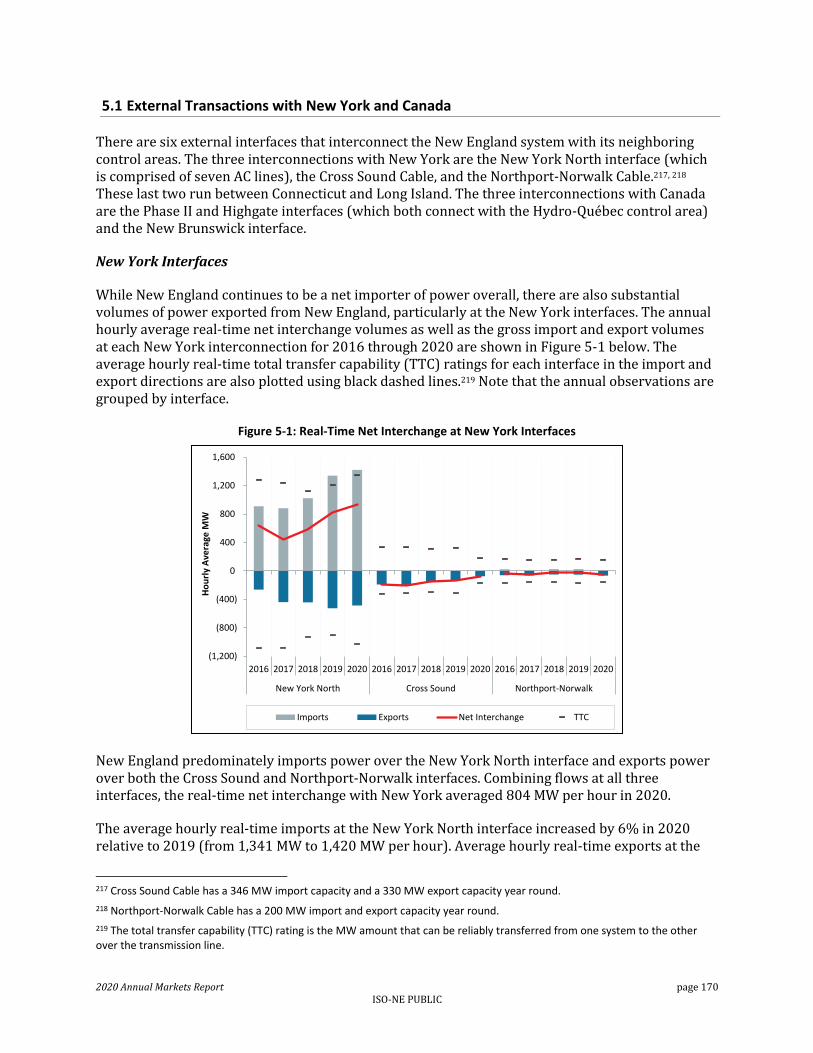
2020 Annual Markets Report page 170 ISO-NE PUBLIC
5.1 External Transactions with New York and Canada
There are six external interfaces that interconnect the New England system with its neighboring control areas. The three interconnections with New York are the New York North interface (which is comprised of seven AC lines), the Cross Sound Cable, and the Northport-Norwalk Cable.217, 218 These last two run between Connecticut and Long Island. The three interconnections with Canada are the Phase II and Highgate interfaces (which both connect with the Hydro-Québec control area) and the New Brunswick interface.
New York Interfaces
While New England continues to be a net importer of power overall, there are also substantial volumes of power exported from New England, particularly at the New York interfaces. The annual hourly average real-time net interchange volumes as well as the gross import and export volumes at each New York interconnection for 2016 through 2020 are shown in Figure 5-1 below. The average hourly real-time total transfer capability (TTC) ratings for each interface in the import and export directions are also plotted using black dashed lines.219 Note that the annual observations are grouped by interface.
Figure 5-1: Real-Time Net Interchange at New York Interfaces
New England predominately imports power over the New York North interface and exports power over both the Cross Sound and Northport-Norwalk interfaces. Combining flows at all three interfaces, the real-time net interchange with New York averaged 804 MW per hour in 2020.
The average hourly real-time imports at the New York North interface increased by 6% in 2020 relative to 2019 (from 1,341 MW to 1,420 MW per hour). Average hourly real-time exports at the
217 Cross Sound Cable has a 346 MW import capacity and a 330 MW export capacity year round.
218 Northport-Norwalk Cable has a 200 MW import and export capacity year round.
219 The total transfer capability (TTC) rating is the MW amount that can be reliably transferred from one system to the other over the transmission line.
(1,200)
(800)
(400)
0
400
800
1,200
1,600
2016 2017 2018 2019 2020 2016 2017 2018 2019 2020 2016 2017 2018 2019 2020
New York North Cross Sound Northport-Norwalk
Ho
url
y A
vera
ge M
W
Imports Exports Net Interchange TTC

2020 Annual Markets Report page 171 ISO-NE PUBLIC
New York North interface decreased for the first time in the reporting period, falling by 7% (from 525 MW to 487 MW per hour). The combined effect was that average hourly net interchange increased by 14% (from 816 MW to 933 MW per hour).
A primary driver of this increase in imports was an increase in the amount of offered supply at low, and even negative, prices. Most notably, participants offered an average of approximately 1,000 MW per hour of imports at fixed or negative prices during the first quarter of 2020. In comparison, approximately 740 MW per hour were offered at fixed or negative prices in 2019 on average. In addition to an increased amount of offered supply at low prices, there were fewer exports cleared at higher prices in 2020. The combination of more supply at lower prices and less external demand at higher prices resulted in higher net interchange.
The average hourly real-time exports at the Cross-Sound Cable interface decreased by 44% in 2020 from 133 MW per hour to 75 MW per hour. This was primarily driven by a reduction in the interface’s TTC during the second half of 2020 due to planned transmission work. Both the import and export TTC’s were restricted to 25% of their typical capacity during this time.
The average hourly net interchange at the Northport-Norwalk interface almost doubled in 2020 from 2019. Net exports averaged 54 MW per hour in 2020 verses 27 MW per hour in 2019, due to an increase in exports and decrease in imports. Average hourly real-time imports decreased by 52% in 2020 from 25 MW per hour to 12 MW per hour, whereas average hourly real-time exports increased by 26%, from 53 MW per hour in 2019 to 66 MW per hour in 2020.
Canadian Interfaces
The annual hourly average real-time net interchange volumes and the gross import and export volumes at each interface with Canada are graphed for each year between 2016 and 2020 in Figure 5-2 below. The average hourly real-time total transfer capability (TTC) ratings for each interface in the import and export directions are also plotted using the black dashed lines.
Figure 5-2: Real-Time Net Interchange at Canadian Interfaces
(1,200)
(800)
(400)
0
400
800
1,200
1,600
2016 2017 2018 2019 2020 2016 2017 2018 2019 2020 2016 2017 2018 2019 2020
Phase II New Brunswick Highgate
Ho
url
y av
era
ge M
W
Imports Exports Net interchange TTC
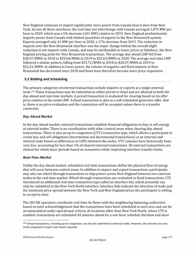
2020 Annual Markets Report page 172 ISO-NE PUBLIC
New England continues to import significantly more power from Canada than it does from New York. Across all three interfaces, the real-time net interchange with Canada averaged 1,876 MW per hour in 2020, which was a 5% decrease (101 MW) relative to 2019. New England predominately imports power from Canada with limited quantities of exports to the New Brunswick system. Exports averaged only 41 MW per hour in 2020, a 17% decrease from 2019. The reduction in imports over the New Brunswick interface was the major change behind the overall slight reduction in net imports with Canada, and may be attributable to lower prices at Salisbury, the New England pricing point for New Brunswick transactions. The average day-ahead LMP fell from $38.47/MWh in 2018 to $29.64/MWh in 2019 to $22.63/MWh in 2020. The average real-time LMP followed a similar pattern, falling from $33.72/MWh in 2018 to $28.07/MWh in 2019 to $22.21/MWh. In addition to lower prices, the volume of negative and fixed imports at New Brunswick has decreased since 2018 and flows have therefore become more price responsive.
5.2 Bidding and Scheduling
The primary categories of external transactions include imports or exports at a single external node.220 These transactions may be submitted as either priced or fixed and are allowed in both the day-ahead and real-time markets. A priced transaction is evaluated for clearing based on its offer price relative to the nodal LMP. A fixed transaction is akin to a self-scheduled generator offer, that is, there is no price evaluation and the transaction will be accepted unless there is a transfer constraint.
Day-Ahead Market
In the day-ahead market, external transactions establish financial obligations to buy or sell energy at external nodes. There is no coordination with other control areas when clearing day-ahead transactions. There is also an up-to congestion (UTC) transaction type, which allows a participant to create buy and sell obligations (incremental and decremental transactions) at an external and internal node based on differences in LMPs between the nodes. UTC volumes have historically been very low, accounting for less than 1% of cleared external transactions. All external transactions are cleared for whole-hour periods based on economics while respecting interface transfer limits.
Real-Time Market
Unlike the day-ahead market, scheduled real-time transactions define the physical flow of energy that will occur between control areas. In addition to import and export transactions, participants may also use wheel-through transactions to ship power across New England between two external nodes in the real-time market. Wheel-through transactions are evaluated as fixed transactions. CTS introduced an additional real-time transaction type called an interface bid, which presently can only be submitted at the New York North interface. Interface bids indicate the direction of trade and the minimum price spread between the New York and New England prices the participant is willing to accept to clear.
The ISO-NE operators coordinate real-time tie flows with the neighboring balancing authorities based on joint acknowledgement that the transactions have been scheduled in each area and can be accommodated under operational criteria. At locations other than New York North, where CTS is enabled, transactions are scheduled 45 minutes ahead for a one-hour schedule duration and must
220 Virtual transactions, including up-to-congestion, can also be submitted at external nodes. However, the volumes are very small compared to export and import volumes.

2020 Annual Markets Report page 173 ISO-NE PUBLIC
be confirmed by the neighboring area. At the CTS location, interface bids are cleared 20 minutes ahead for 15-minute schedules.221
External transactions clearing in the day-ahead and real-time markets occur independently, although a single transaction can have day-ahead and real-time offers. A cleared day-ahead transaction does not automatically carry over to real-time; the participant must elect to also submit the transaction in real-time or may choose to offer the transaction only in real-time. When a participant does submit a transaction with both day-ahead and real-time offers, there is some scheduling priority afforded during real-time. In particular, the day-ahead MW-amount cleared is scheduled as if it were offered as a fixed transaction in real-time unless the participant alters the offer price or withdraws the transaction in real-time.222
New York Interfaces
The composition of day-ahead and real-time cleared transactions (both imports and exports) at the New York interfaces is charted in Figure 5-3 below for each year between 2016 and 2020.223 The lighter yellow series illustrates the total volume of cleared fixed transactions; the percentage is the share of overall cleared transactions that were fixed. The darker yellow series illustrates the volume of cleared priced transactions. The volumes presented represent the annual average MW volumes per hour for each year.
Figure 5-3: Cleared Transactions by Market and Type at New York Interfaces
Due to the implementation of CTS at the New York North interface in December 2015, a large percentage of New York real-time transactions shifted from fixed to priced in 2016. This trend continued over the reporting period as the percentage of New York real-time fixed transactions fell to only 11% in 2020, the lowest percentage of the last five years. Due to CTS, all real-time transactions at New York North are now evaluated based on price, although participants may offer
221 The clearing process begins 45 minutes before the 15-minute interval and ends 20 minutes before.
222 This scheduling priority is not applicable to real-time interface bids at CTS locations.
223 Refer to Section 2.3 for details of the external nodes associated with the New York, Québec, and New Brunswick.
64% 54% 38% 55% 61% 36% 32% 17% 13% 11%
0
500
1,000
1,500
2,000
2,500
2016 2017 2018 2019 2020 2016 2017 2018 2019 2020
Day-ahead Real-time
Ho
url
y av
era
ge M
W
Priced
Fixed

2020 Annual Markets Report page 174 ISO-NE PUBLIC
prices as low as -$1,000/ MWh to effectively schedule the transaction as fixed. The percentage of day-ahead priced transactions at the New York interfaces fell in 2020 from 45% to 39%, consistent with 2016 but slightly higher than 2017-2019 outcomes.
The breakout of fixed and priced transactions by directional flow at the New York interfaces is shown in Table 5-1 below. The values presented in this table are for cleared transactions and the volumes are the average MW per hour.
Table 5-1: Transaction Types by Market and Direction at New York Interfaces (Average Cleared MW per hour)
Market Direction Type 2016 2017 2018 2019 2020
Day-ahead
Import
Priced (MW) 133 195 447 323 308
Fixed (MW) 709 577 441 699 815
Priced (%) 16% 25% 50% 32% 27%
Fixed (%) 84% 75% 50% 68% 73%
Export
Priced (MW) 298 375 354 268 227
Fixed (MW) 48 101 54 21 17
Priced (%) 86% 79% 87% 93% 93%
Fixed (%) 14% 21% 13% 7% 7%
Real-time
Import
Priced (MW) 651 657 967 1,281 1,265
Fixed (MW) 281 234 82 86 168
Priced (%) 70% 74% 92% 94% 88%
Fixed (%) 30% 26% 8% 6% 12%
Export
Priced (MW) 272 436 442 536 563
Fixed (MW) 242 272 205 175 65
Priced (%) 53% 62% 68% 75% 90%
Fixed (%) 47% 38% 32% 25% 10%
Most day-ahead hourly cleared export transactions at the New York interfaces tend to be priced, while most imports tend to be fixed. In 2020, 27% of the average hourly cleared day-ahead import transactions at the New York interfaces were priced transactions (308 MW per hour). This represents a 5% decrease on 2019. Conversely, the majority of day-ahead export transactions at the New York interfaces continued to be priced. The percentage of priced export transactions remained constant at 93% in 2020.
When breaking out day-ahead cleared volume further by type, Table 5-1 highlights the continuing trend of imports comprising the majority of fixed cleared volumes. Imports accounted for 82% of hourly average cleared MW volumes in the day-ahead market. This is slightly higher than in 2019, when 78% of cleared MW per hour were imports. Imports into New England are generally less price-sensitive than exports from New England. One possible explanation for this continued behavior is contractual positions that participants have entered into prior to the delivery day, or eligibility for renewable energy credits in the New England states.
In the real-time market, the majority transaction volumes continued to be priced transactions, on average. Table 5-1 shows a trend of increases in priced imports and exports over the entire reporting period. In 2020 the average volume of real-time fixed imports also increased from 86 MW in 2019 to 168 MW in 2020. This increase is approximately double the 2018 and 2019 volumes but only accounts for 12% of imports.
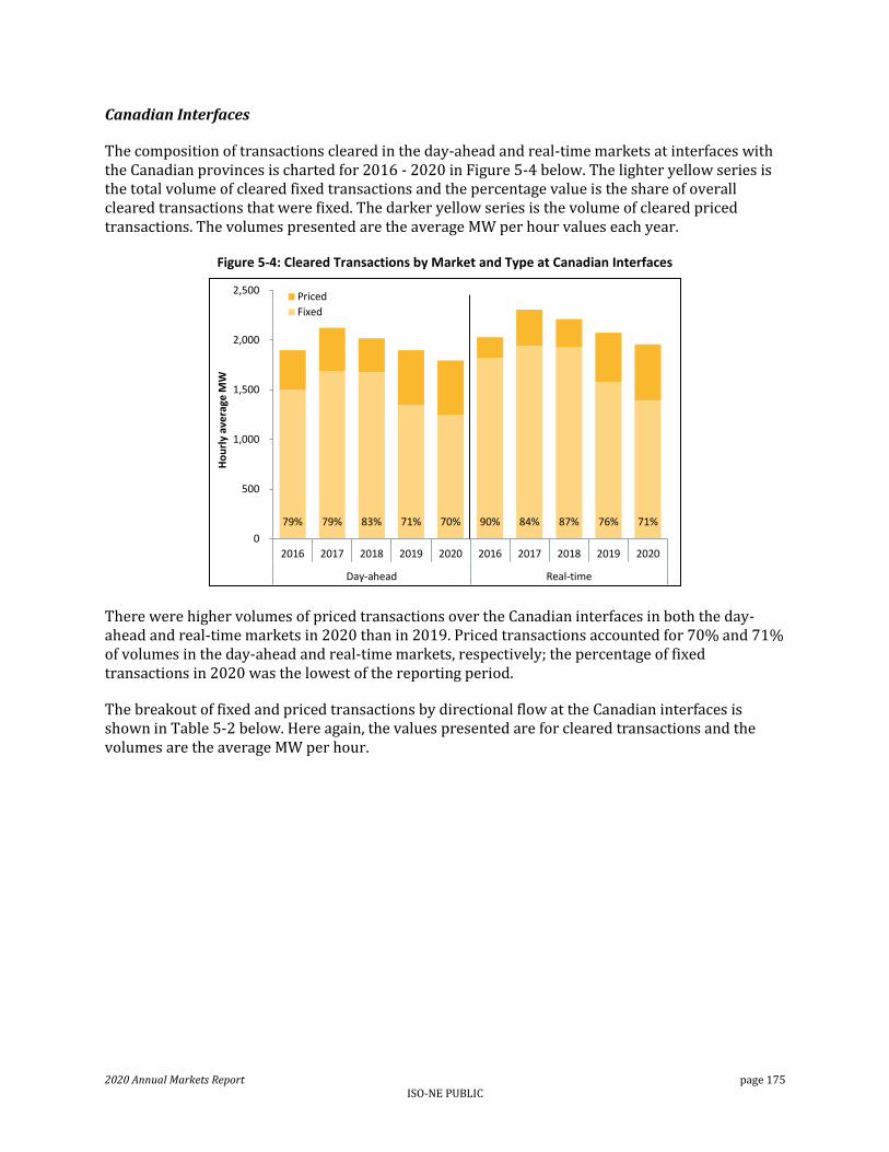
2020 Annual Markets Report page 175 ISO-NE PUBLIC
Canadian Interfaces
The composition of transactions cleared in the day-ahead and real-time markets at interfaces with the Canadian provinces is charted for 2016 - 2020 in Figure 5-4 below. The lighter yellow series is the total volume of cleared fixed transactions and the percentage value is the share of overall cleared transactions that were fixed. The darker yellow series is the volume of cleared priced transactions. The volumes presented are the average MW per hour values each year.
Figure 5-4: Cleared Transactions by Market and Type at Canadian Interfaces
There were higher volumes of priced transactions over the Canadian interfaces in both the day-ahead and real-time markets in 2020 than in 2019. Priced transactions accounted for 70% and 71% of volumes in the day-ahead and real-time markets, respectively; the percentage of fixed transactions in 2020 was the lowest of the reporting period.
The breakout of fixed and priced transactions by directional flow at the Canadian interfaces is shown in Table 5-2 below. Here again, the values presented are for cleared transactions and the volumes are the average MW per hour.
79% 79% 83% 71% 70% 90% 84% 87% 76% 71%
0
500
1,000
1,500
2,000
2,500
2016 2017 2018 2019 2020 2016 2017 2018 2019 2020
Day-ahead Real-time
Ho
url
y av
era
ge M
W
Priced
Fixed

2020 Annual Markets Report page 176 ISO-NE PUBLIC
Table 5-2: Transaction Types by Market and Direction at Canadian Interfaces (Average MW per hour)
Market Direction Type 2016 2017 2018 2019 2020
Day-ahead
Import
Priced (MW) 399 418 327 544 529
Fixed (MW) 1,491 1,677 1,667 1,336 1,242
Priced (%) 21% 20% 16% 29% 30%
Fixed (%) 79% 80% 84% 71% 70%
Export
Priced (MW) 2 18 12 10 16
Fixed (MW) 6 11 12 8 8
Priced (%) 22% 61% 50% 56% 69%
Fixed (%) 78% 39% 50% 44% 31%
Real-time
Import
Priced (MW) 203 354 275 487 559
Fixed (MW) 1,788 1,871 1,859 1,539 1,358
Priced (%) 10% 16% 13% 24% 29%
Fixed (%) 90% 84% 87% 76% 71%
Export
Priced (MW) 4 13 10 8 6
Fixed (MW) 35 69 69 41 34
Priced (%) 10% 16% 12% 16% 16%
Fixed (%) 90% 84% 88% 84% 84%
Both imports and exports at the Canadian interfaces continue to be predominantly fixed. Similar to the decrease in both day-ahead and real-time prices at Salisbury stated above, prices at Phase II have also continued to fall since 2018. The average day-ahead LMP fell from $43.45/MWh in 2018 to $23.08/MWh in 2020. The average real-time LMP followed a similar pattern, falling from $42.80/MWh in 2018 to $23.11/MWh. This decrease in LMP might be prompting participants to be more price sensitive.
5.3 External Transaction Uplift (Net Commitment Period Compensation) Credits
The ISO lacks sufficient information to calculate day-ahead or real-time congestion prices at non-CTS external nodes (i.e., the marginal cost of power on the other side of the interface).224 Instead, the cost of relieving congestion is reflected in a transfer of uplift payments between those causing the congestion and those relieving the congestion.
Uplift payments accrue in the day-ahead market when fixed import or export transactions exceed the TTC of the interface and offsetting interchange transactions (withdrawals or injections over the interface) are cleared to create counter-flow for the fixed transactions to clear. The participant with the offsetting transaction that provided the counter-flow receives the uplift and the participant with the fixed transaction that was allowed to clear is charged the uplift.
Absent congestion pricing, the day-ahead market applies a nodal constraint that limits the net injections at an external node to the transfer capability of the corresponding external interface. Offsetting injections (import transactions and virtual supply) and withdrawals (export transactions and virtual demand) will be cleared so long as the interface limit is not exceeded. This means, for example, that a total volume of import transactions or virtual supply offers that exceed the import transfer capability can be cleared so long as offsetting export transactions or virtual demand bids are available. The clearing of these offsetting transactions does not affect the nodal LMP.
224 Prior to CTS, this was the case at all external nodes. However, congestion pricing has been implemented for the New York North external node in both the day-ahead and real-time markets since December 2015, coincident with CTS implementation.

2020 Annual Markets Report page 177 ISO-NE PUBLIC
Similar to generator out-of-merit credits, real-time uplift credits at external nodes are paid to priced transactions that prove to be out-of-merit for the hour. In the real-time energy market, external transactions are scheduled based on a comparison of the transaction price to the ISO-NE forecasted price for the external node.225 If the actual real-time LMP for an external node is less than the offer price of a cleared import transaction at that node, the participant will receive uplift payments to be made whole to its offered price. Conversely, if the actual real-time LMP for an external node is more than the bid price of a cleared export transaction at that node, the participant will receive uplift payments to be made whole to its bid price. Real-time uplift payments to external transactions are only paid to priced transactions – fixed transactions are willing to clear at any price, and therefore cannot clear out-of-merit.
The annual uplift credit totals at all external nodes in both the day-ahead and real-time markets for each year from 2016 through 2020 are presented in Table 5-3 below.
Table 5-3: NCPC Credits at External Nodes
Year Day-ahead credits
($ million) Real-time credits
($ million)
2016 $0.90 $1.28
2017 $0.56 $1.92
2018 $0.30 $2.73
2019 $0.02 $1.02
2020 $0.00 $1.39
The total amount of uplift credits paid at external nodes is very small compared with other types of uplift (see Section 3.5). In the day-ahead market, we typically see these payments occur when there is a large decrease in an interface TTC until participants adjust their fixed bidding behavior.
Day-ahead uplift credits at external nodes decreased 95% in 2020 compared to 2019, falling to just over one thousand dollars. As
Table 5-3 shows, total real-time external transaction uplift credits during 2020 were 37% higher than in 2019. The increase in payments was seen primarily at the Phase II interface, where payments increased by 123% from $172 thousand to $384 thousand. The majority of external uplift payments, 58%, continue to be paid out over the New Brunswick interface. These payments increased slightly from $697 thousand in 2019 to $808 thousand in 2020. These increases in payments over the Phase II and New Brunswick interfaces were driven by price forecasting errors.
5.4 Coordinated Transaction Scheduling
The Coordinated Transaction Scheduling (CTS) mechanism is intended to improve the efficiency of real-time energy trades between New England and New York. CTS was implemented by ISO-NE and the New York Independent System Operator (NYISO) in December 2015, for the New York North interface. The design modified the bidding and scheduling mechanics for real-time transactions. The design changes unified the bid submission and clearing process, decreased the schedule 225 This is for non-CTS interfaces. For New York North (the only CTS interface) real-time interface bids are cleared based on forecasted price differences between NYISO and ISO-NE.

2020 Annual Markets Report page 178 ISO-NE PUBLIC
duration from one hour to 15-minute intervals, moved bid submittal and clearing timelines closer to the interval when power flows, and eliminated transaction fees.226 The CTS design was intended to improve the extent to which power moves from the lower- to higher-cost region and increase the utilization of interface transfer capability to better converge prices between the regions.
CTS Scheduled Flow in the Correct Direction 55% of time in 2020
Average annual data on CTS scheduled flows are presented in Table 5-4 below and indicates a worsening performance of CTS. The table shows the percentage of real-time intervals when the net CTS flows were in either the New England or New York direction, and the percentage of real-time intervals when the flows were in the economically correct direction (i.e. from lower-cost to higher-cost market). The latter statistic is shown based on the forecasted price difference (relevant to the actual clearing of CTS bids), as well as on the actual settled prices.
Table 5-4: Summary of CTS Outcomes
Net Flow (% of intervals), to: Correct Flow (% of intervals), based on:
Year ISO-NE NYISO Forecast Spread Actual Spread
2016 94% 6% 63% 56%
2017 79% 20% 68% 61%
2018 88% 12% 59% 63%
2019 94% 6% 47% 58%
2020 97% 3% 39% 55%
In 2020, New England was a net importer during 97% of real-time intervals, the highest level of the entire reporting period. Overall, CTS bids in 2020 allowed power to flow consistent with forecasted price differences only 39% of the time, which was down from 47% observed in 2019. Based on actual price differences, power flowed in the correct direction 55% of the time, which was slightly worse than the 58% observed in 2019. This trend is consistent with the increase in negative import spread bids into New England in recent years. Negative import spread bids are scheduled even when power is being imported from the higher-cost region to a lower-cost region. This type of bidding behavior is discussed more in the section below.
CTS Transactions Continue to Flow in the Uneconomic Direction due to Bidding Behavior
The bid types submitted by participants over the CTS interface heavily affect the ability of the CTS design to schedule real-time power efficiently. The process can only schedule volumes up to the amount of the bid volumes submitted and at the price up to the forecasted price spread. Bid prices can be positive, negative, or zero. A positive bid price indicates the participant is willing to move power when, as forecasted, the price in the destination market exceeds the price in the source market by at least the bid price (i.e., buy low and sell high). A negative bid price indicates a willingness to trade power even when the energy price is higher at the source than at the destination, by as much as the negative bid price (i.e., to counterintuitively buy high and sell low).
Average CTS transaction curves, by year, are shown in Figure 5-5 below. Import offers are shown in the first graph (gold curves) followed by export bids (red curves). Lastly, imports and exports are
226 The design basis documents, FERC filing materials, and implementation documentation describing the CTS design in detail can be found on the ISO-NE key project webpage: http://www.iso-ne.com/committees/key-projects/implemented/coordinated-transaction-scheduling/

2020 Annual Markets Report page 179 ISO-NE PUBLIC
aggregated to produce a net supply curve (orange curves). The import and export curves show the average volume of energy willing to clear at each New England - New York price spread. The aggregate supply curve shows the net flow that would be produced if all of the economic import and export transactions cleared. The darker-colored lines show the 2020 curves and lighter colored lines show the 2019 curves. The x-axis shows the spread of New England and New York prices – positive numbers indicate that New England prices are higher. When New England prices are higher (i.e. the price spread is positive), the expectation is that more imports and less exports would be willing to clear. The y-axis shows the volume of energy that would clear, on average, at each price spread.
For example, in 2020, at a price spread of $0/MWh, 1,273 MW of imports would have cleared, 269 MW of exports would have cleared, and the net flow of CTS transactions would have been 1,005 MW, on average.
Figure 5-5: Price Sensitivity of Offered CTS Transactions
There were two points along the supply curve with notable changes in offered import volumes at negative price spreads. First there was a 40 MW increase at very low price spreads (-$50/MWh) in
0
500
1,000
1,500
2,000
-$50 $0 $50
Av
era
ge O
ffe
red
Im
po
rts
(MW
)
Willing to clear at a loss
0
300
600
900
1,200
1,500
-$50 $0 $50
Ave
rage
Off
ere
d
Exp
ort
s (M
W)
2019 vs. 2020
Willing to clear at a loss
-600
0
600
1,200
1,800
-$50 $0 $50
Ave
rage
Ne
t O
ffe
red
Im
po
rts
-Ex
po
rts
(MW
)
New England - New York Price Difference
2019 vs. 2020
New England Price HigherNew York Price Higher
Will
ing
to N
et
Imp
ort
Will
ing
to N
et
Exp
ort
2019 vs. 2020
Import Supply Curve
Export Demand Curve
Net Supply Curve (Imports - Exports)
2020 Annual Markets Report page 180 ISO-NE PUBLIC
2020 compared with 2019. In addition, at a price spread of -$20/MWh there was an increase in offered volumes of 90 MW. On the positive spreads bid side import offers between $5 and $25/MWh also increased by an average of about 120 MW.
Meanwhile, export bids that were willing to move power at higher New England prices (spread of $50/MWh) decreased by 30 MW between 2019 and 2020 (these bids are indicative of export transactions that are willing to export power from New England even when the New England price is $50/MWh greater than the New York price). While the shift in the export demand curve allowed for slightly less flow in the correct direction, this was mostly offset by opposite impact of the import supply curve shift. In other words, the aggregate supply curve allowed the direction of flows to be less consistent with price differences than in the prior year, on average. Therefore, in 2020 more net imports were scheduled to flow into New England at a loss than in 2019.
In 2019, market participants were willing to export energy to New York only when New York prices were at least $11/MWh higher (see the intersection of the 2019 net supply curve at 0 MW), on average. Or conversely, participants were willing to move the flow to the net import direction into New England even at a loss of $11/MWh. This trend in uneconomic power flow continued to worsen in 2020, when participants were only willing to export power to New York when New York prices were at least $16/MWh higher, on average. One possible explanation for this bidding behavior (willing to flow energy at a loss) may be due to contractual positions that some participants entered into prior to the delivery day, or eligibility for renewable energy credits in the New England states.
Price Convergence in 2020 Comparable to 2019
To examine the degree of real-time price convergence achieved under the CTS design relative to prior years, we examine two main factors: (1) the percent difference of the average hourly real-time price between the two control areas, and (2) the level of volatility in each area. 227 These two metrics are provided in Figure 5-6 below. Percentage differences are used to adjust for absolute price levels.228 The line series in Figure 5-6 plot the cumulative distribution function for observations of the absolute percentage difference between the ISO-NE and NYISO real-time hourly energy prices at the New York North interface.
In the chart below, the vertical axis represents the absolute percentage difference in price at each side of the interface. The horizontal axis represents the probability of a price difference at that percentage or less. For example, at a 10% absolute price difference (on the vertical axis), scanning horizontally to the right, the 2020 line corresponds to a horizontal axis value of 36%. This means that 36% of hours in 2020 had an absolute price difference between the control areas of 10% or less. To help compare across years, the table embedded in the chart provides the probabilities of a few price difference values (i.e., 10%, 25%, 50%) for each year.
To describe the relative market price volatility in each of these years, the table in Figure 5-6 also includes the coefficient of variation for real-time energy prices. The coefficient of variation measures how much each ISO’s real-time price varied relative to its average price for the year.229 The lower the price volatility the more we would expect to observe New England and New York 227 The NYISO pricing node is called “N.E._GEN_SANDY PD” and the ISO-NE node is “.I.ROSETON 345 1.”
228 Higher absolute prices often result in larger price differences. Percentage differences are shown so that larger magnitude price differences due to higher absolute prices are not attributed to CTS.
229 The coefficient of variation is the ratio of the standard deviation to the mean.

2020 Annual Markets Report page 181 ISO-NE PUBLIC
prices remaining close to one another. When price volatility is higher, a greater degree of price divergence between the regions is expected, unless a scheduling system like CTS is frequently adjusting the interface flow.
Figure 5-6: New York North Real-Time Price Difference between ISO-NE and NYISO
Figure 5-6 indicates that price convergence in 2020 was very close to 2019 levels, in the context of slight lower price volatility in both markets. New York and New England prices were within 25% of each other over 70% of the time, and within 50% of each other over 90% of the time.
The current reporting year continued the trend of more stable prices in each control area. In 2020, the coefficient of variation in real-time prices was 59% for ISO-NE, the lowest value since the implementation of CTS. Similarly, on the NYISO side, the coefficient of variation in real-time prices was 64%. This is consistent with the New York North interface binding with smaller marginal values (less congestion) as well as the New England system experiencing no extreme events or scarcity conditions that increased prices. The lack of extreme system events is further explained in Section 3.4.8.
Price Forecast Error may be Continuing to Inhibit CTS Effectiveness
The efficiency of CTS schedules can be impacted by the accuracy of the ISOs’ internal price forecasts for the relevant external nodes. Price forecasts are calculated for each 15-minute interval and used to determine which participant bids clear and the interface net flow. Interface bids clear if the offer price is below the forecasted price difference. ISO-NE creates its CTS price forecast using current offers and system conditions at about 45 minutes ahead of the scheduling interval. The NYISO forecasts its internal price at about 30 minutes ahead of the scheduling interval. A summary of forecast versus actual prices, as well as the average and absolute forecasting errors, is provided in Table 5-5 below.
0%
50%
100%
150%
200%
250%
0% 10% 20% 30% 40% 50% 60% 70% 80% 90% 100%
Per
cen
t d
iffe
ren
ce b
etw
een
ISO
-NE
and
NY
ISO
pri
ces
Percent of Observations
2016
2017
2018
2019
2020
Downward shift of the duration curve (flatter curve) would indicate improvedprice convergence - convergence remained constant in 2020 (green line) compared to 2019 (red line)
2016 2017 2018 2019 2020
Under 10% 29% 35% 36% 37% 36%
Under 25% 60% 65% 67% 72% 71%
Under 50% 83% 86% 88% 91% 91%
ISO-NE LMP 117% 84% 98% 62% 59%
NYISO LBMP 106% 95% 118% 65% 64%
RT LMP
% difference Percent of observations
Coefficient of variation (σ/µ)

2020 Annual Markets Report page 182 ISO-NE PUBLIC
Table 5-5: Pricing and Forecast Error Statistics in the CTS Solution
Forecast LMP Actual LMP Average Forecast Error
Average Absolute Forecast Error
ISO-NE NYISO Spread ISO-NE NYISO Spread ISO-NE NYISO Spread ISO-NE NYISO Spread
(a) (b) (c)=(a)-(b) (d) (e) (f)=(d)-(e) (f)=(a)-(d) (g)=(b)-(e) (h)=(c)-(f) (i) (j) (k)
2016 $28.82 $27.66 $1.16 $28.02 $29.23 ($1.22) $0.80 ($1.58) $2.38 $8.47 $6.61 $12.29
2017 $33.37 $31.29 $2.08 $32.02 $32.37 ($0.34) $1.34 ($1.08) $2.42 $8.18 $6.84 $12.32
2018 $38.21 $38.99 ($0.77) $39.29 $40.80 ($1.51) ($1.07) ($1.81) $0.74 $8.09 $8.45 $13.49
2019 $26.69 $28.79 ($2.09) $27.71 $28.43 ($0.72) ($1.02) $0.36 ($1.37) $4.69 $5.07 $7.97
2020 $20.39 $22.65 ($2.27) $21.12 $21.79 ($0.66) ($0.74) $0.87 ($1.60) $3.76 $4.04 $6.34
CTS transactions are scheduled on a forecasted spread basis.230 The average forecast error, which considers directionality, captures the offsetting or compounding effect of each control area’s forecast error. The forecasted ISO-NE/NYISO spread continued to signal higher NY prices (at the Sandy Pond node), with an average forecasted spread of $2.27/MWh (column c). The higher NY price spread was also reflected in actual settled prices, with an average actual spread of $0.66/MWh (f). ISO-NE’s average forecast error (at Roseton) improved from -$1.02/MWh (negative indicating lower than actual forecasted prices) in 2019 to -$0.74/MWh in 2020. In other words, at Roseton the forecasted price continued to be lower than the actual price, but the error was smaller in 2020. However, the improvement was offset by the NYISO average error, with forecasted price $0.87/MWh more than the actual price (g). The combined effect of the forecast error resulted in an actual NE/NY spread that was $1.60/MWh lower than forecasted (-$0.66 actual vs, $-2.27 forecasted, with negative indicating lower ISO-NE prices).
Absolute forecast error ignores directionality of the error and focuses on magnitude. This error is calculated by averaging the absolute difference between the forecasted and actual LMPs in each ISO. Similarly, the average absolute price spread difference is calculated by averaging the absolute difference between spread prices and is shown in column (k). In 2020 both ISOs’ had the smallest average absolute forecast error since the implementation of CTS. This downward trend of average absolute error indicates that the difference between the forecasted LMPs and the actual LMPs is decreasing. Likewise, the spread average absolute forecast error had decreased since 2018, indicating that the forecasted and actual spread prices are getting closer.
Forecast performance remains inconsistent for both Roseton and Sandy Pond across many hours of the day. Figure 5-7 below shows the simple average of forecast errors for 2020 calculated by hour of the day (yellow bars). A positive observation in Figure 5-7 indicates the forecast price is higher than the actual price and a negative observation indicates the forecast price is lower than actual price. The red line series represents the average error in the New York price forecast for each hour and the blue line series represents the average error in the New England price forecast each hour.
230 Price difference forecast error is: (Forecast New England – Forecast New York) – (Actual New England – Actual New York).
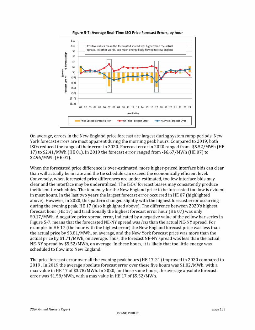
2020 Annual Markets Report page 183 ISO-NE PUBLIC
Figure 5-7: Average Real-Time ISO Price Forecast Errors, by hour
On average, errors in the New England price forecast are largest during system ramp periods. New York forecast errors are most apparent during the morning peak hours. Compared to 2019, both ISOs reduced the range of their error in 2020. Forecast error in 2020 ranged from -$5.52/MWh (HE 17) to $2.41/MWh (HE 01). In 2019 the forecast error ranged from -$6.67/MWh (HE 07) to $2.96/MWh (HE 01).
When the forecasted price difference is over-estimated, more higher-priced interface bids can clear than will actually be in rate and the tie schedule can exceed the economically efficient level. Conversely, when forecasted price differences are under-estimated, too few interface bids may clear and the interface may be underutilized. The ISOs’ forecast biases may consistently produce inefficient tie schedules. The tendency for the New England price to be forecasted too low is evident in most hours. In the last two years the largest forecast error occurred in HE 07 (highlighted above). However, in 2020, this pattern changed slightly with the highest forecast error occurring during the evening peak, HE 17 (also highlighted above). The difference between 2020’s highest forecast hour (HE 17) and traditionally the highest forecast error hour (HE 07) was only $0.17/MWh. A negative price spread error, indicated by a negative value of the yellow bar series in Figure 5-7, means that the forecasted NE-NY spread was less than the actual NE-NY spread. For example, in HE 17 (the hour with the highest error) the New England forecast price was less than the actual price by $3.81/MWh, on average, and the New York forecast price was more than the actual price by $1.71/MWh, on average. Thus, the forecast NE-NY spread was less than the actual NE-NY spread by $5.52/MWh, on average. In these hours, it is likely that too little energy was scheduled to flow into New England.
The price forecast error over all the evening peak hours (HE 17-21) improved in 2020 compared to 2019 . In 2019 the average absolute forecast error over these five hours was $1.82/MWh, with a max value in HE 17 of $3.78/MWh. In 2020, for those same hours, the average absolute forecast error was $1.58/MWh, with a max value in HE 17 of $5.52/MWh.
($12)
($10)
($8)
($6)
($4)
($2)
$0
$2
$4
$6
$8
$10
$12
01 02 03 04 05 06 07 08 09 10 11 12 13 14 15 16 17 18 19 20 21 22 23 24
Fore
cast
Lo
w ←
→
Fo
reca
st H
igh
Price Spread Forecast Error NY Price Forecast Error NE Price Forecast Error
Hour Ending
$/M
Wh
Positive values mean the forecasted spread was higher than the actualspread. In other words, too much energy likely flowed to New England

2020 Annual Markets Report page 184 ISO-NE PUBLIC
Section 6 Forward Capacity Market
This section reviews the performance of the forward capacity market (FCM), including key trends in resource participation, auction prices and auction competiveness.
Overall, the FCM has achieved its design objectives of attracting new efficient resources, maintaining existing resources and sending price signals for the retirement of less efficient resources. Capacity prices resulting from the forward capacity auctions (FCAs) have increased and decreased as the number of resources competing and clearing in the auctions and the region’s surplus capacity has changed. However, ensuring competitive pricing outcomes in the FCM is becoming increasingly challenging and the ISO and stakeholders have been working on exploring innovative solutions to these challenges.
The first challenge has been to accommodate new resources, which secure revenue through state-backed programs designed primarily to meet state environmental and climate goals – these so-called “out-of-market” revenues can lead to market distortions and price suppression. The Minimum Offer Price Rules (MOPR) are designed to mitigate the impact of new supply offers below competitive levels, and in practice apply to a large extent to state-subsidized resources that are being developed to meet the states’ environmental goals. The exclusion of such out-of-market revenues means that such resources are less likely to clear in the FCAs, which does not align with the states’ goals of achieving future emissions targets.
For FCA 13, the ISO introduced Competitive Auctions with Sponsored Policy Resources (CASPR) to help address this issue. CASPR provides a market-based mechanism for state-sponsored resources to replace retiring generation in the FCM while maintaining competitive prices in the primary auction. However, while the price-suppressing impact is mitigated in the first year, the sponsored resources will likely be price-takers in subsequent auctions thereby applying downward pressure to future FCA clearing prices in the long-term. This underlying compromise behind the CASPR design is unavoidable so long as resources receive out-of-market revenues. Also, while CASPR and the current market power mitigation rules help mitigate the impacts on new resources, they do not address the impact of out-of-market revenues paid to retain existing resources, when they might otherwise retire.
The second challenge is the reliability retention of FCM resources based on their underlying energy-security attributes; attributes that are not reflected in the current FCM or energy market designs. Once such an attribute becomes scarce and impacts market outcomes, it is important from a market efficiency perspective to value it appropriately in the wholesale market. To that end, the ISO worked with stakeholders on designing new reserve products to be procured in the day-ahead market, with the objective of valuing and compensating resources for providing energy security. This new rules were proposed to be implemented in June 2024.231 In late 2020, FERC rejected proposed market rules changes in their entirety.232 The Interim Compensation Treatment mechanism will be in place for FCA 14 and 15 as means for compensating resources for their energy
231 See ER20-1567-000; Energy Security Improvements Compliance Filing, April 15, 2020 at https://www.iso-ne.com/static-
assets/documents/2020/04/energy_security_improvements_filing.pdf
232 See ER20-1567-000 Order Rejecting Energy Security Improvements, October 30, 2020 at https://www.iso-ne.com/static-
assets/documents/2020/10/er20-1567-000_order_rejecting_esi_10-30-2020.pdf

2020 Annual Markets Report page 185 ISO-NE PUBLIC
security attributes. However, beyond this there is no mechanism – administrative or market based – in place that will explicitly values energy or fuel security attributes in an increasingly energy constrained system.
Summary of FCA Trends Covered in this Section
The first seven FCAs, for the commitment periods between June of 2010 through May of 2017, experienced relatively stable capacity prices resulting from surplus capacity and administrative price-setting rules. In contrast, in FCA 8 the retirement of over 2,700 MW of older nuclear, coal- and oil-fired generators reduced the region’s capacity surplus and produced higher capacity prices. Payments for capacity commitment period (CCP) 8 reached $3 billion, a 162% increase in payments from prior commitment period ($1.2 billion).
The trend of minimal surplus and increased capacity payments continued into 2018-19. As capacity prices increased, new suppliers entered the market in FCAs 9 and 10 and increased the amount of system capacity, leading to a decline in prices. This pattern of increasing prices followed by decreasing prices is what one would expect in a market that is gaining new and losing older generators as it oscillates around an equilibrium. Further, planned transmission improvements, coupled with an increase in the number of resources competing in the auctions, increased the capacity market’s overall competitiveness. FCAs 11-14 saw continuous decreases of clearing prices even absent of significant new entry.
The clearing price in the most recent auction, FCA 15, was $2.61/kW-month in the Rest-of-Pool capacity zone, $3.98/kW-month in the Southeastern New England capacity zone, and $2.48/kW-month in the Northern New England capacity zone. The price separation in these zones reflects the export- and import-constrained nature of certain areas in the New England grid. Payments are expected to reach $1.4 billion for FCA 15, $0.4 billion higher than the record low payments expected for FCA 14. FCA 15 marked the first auction without the Mystic 8 and 9 generators, two LNG-supplied combined cycles in Boston that were retained for reliability due to their fuel-security attributes under a FERC-approved cost-of-service agreement. That agreement ended in FCA 15, leading to a 1,400 MW departure of qualified capacity in the Southeastern New England capacity zone. Additionally, a total of 1,287 MW de-listed from the auction, with 767 MW (60%) from gas-fired resources and 187 MW (15%) from oil-fired resources retiring. New cleared capacity replaced 1,121 MW, with the largest portion of new capacity being supplied by battery storage projects (600 MW). This section is structured as follows:
Section 6.1 provides a high-level overview of the market design, summarizing resource qualification, auctions mechanics and performance incentives.
Section 6.2 summarizes overall payments made to capacity resources, including adjustments such as peak energy rent, shortage event penalties, and pay-for-performance.
Section 6.3 summarizes the inputs and outcomes of the most recent forward capacity auction, FCA 15.233
Section 6.4 reviews key trends in primary (FCA) and secondary capacity trading. Section 6.5 focuses on trends in the resource mix and the major new entry and exit of
resources that have shaped those trends.
233 A more detailed review of FCA 15 is covered in the IMM Winter 2020/2021 Quarterly Markets Report, at https://www.iso-ne.com/static-assets/documents/2021/04/2021-winter-quarterly-markets-report.pdf
2020 Annual Markets Report page 186 ISO-NE PUBLIC
Sections 6.6 and 6.7 present metrics on the structural competiveness of the FCAs. They also describe mitigation measures in place to address the potential exercise of market power, and provide statistics on the extent to which uncompetitive offers were mitigated.
6.1 Forward Capacity Market Overview
The FCM is designed to achieve several market and resource adequacy objectives. First, the FCM provides developers of new resources and owners of existing resources an additional revenue source. The FCM or “capacity” revenue is intended to offset the revenue shortfall or “missing money” that arises as a result of marginal-cost bidding and administrative offer caps in the energy market. Second, a developer or owner will know their capacity payment rate ($/kW-month) for the first year of commercial operation in advance of starting construction of a new resource or making a significant capital investment in an existing resource. Third, the FCM provides all owners (of a new or existing resource) with financial incentives to operate and maintain their resource so it is available during system shortage conditions. Finally, the FCM’s descending clock auction is designed to produce a market-based price for capacity by selecting the least-cost set of qualified supply resources that will satisfy the region’s price-sensitive demand needs.
The FCM provides Additional Revenue to Capacity Developers and Owners
If New England’s energy markets included sufficiently high scarcity pricing, resource owners would have the opportunity to earn infra-marginal rents (the difference between energy market prices and their resource’s variable costs) to cover fixed costs, earn reasonable profits, and gain return on capital investments in the long run. Marginal-cost bidding and energy market offer caps intrinsically limit energy market prices and disallow investors to reap significant profits in the energy market and cover fixed costs unrelated to generation. The gap between the revenue developers need to justify capital investments and the revenue available to fund those investments is denoted as “missing money.” This “missing money” is referred to in several specific terms used throughout this report, including Net Cost of New Entry (Net CONE), Offer Review Trigger Prices (ORTPs), offer floor prices, net going-forward costs, and de-list bids.
The FCM’s capacity prices and revenues facilitate efficient entry and exit decisions. That is, the market should attract new resources, maintain competitively-priced resources, and retire uncompetitive resources while meeting the region’s resource adequacy standard in the most cost-effective manner. In FCA 13, this was not the case. Mystic 8 and 9 were retained for fuel security within the Southeastern New England capacity zone, and entered into a cost-of-service agreement with the ISO.234 The agreement suggests that the FCA could not facilitate an efficient and reliable solution. In FCA 15, the cost-of-service agreement ended due to accepted transmission proposals and updated fuel security reviews, allowing Mystic 8 and 9 to retire effective June 1, 2024.235
The FCM provides Resource Owners with Certainty about Future Payments
The FCM procures capacity through an auction mechanism 40 months in advance of when it must be delivered in the energy markets. The delivery period is known as the capacity commitment period (CCP). A resource that successfully sells its capacity in the auction assumes a capacity supply
234 For more information on the fuel security order see: https://www.iso-ne.com/static-assets/documents/2018/12/fuel_security_order.pdf
235 For more information on the end of the Mystic 8 and 9 cost-of-service agreement, see: https://www.iso-ne.com/static-assets/documents/2020/08/a7_fca_15_transmission_security_reliability_review_for_mystic_8_9.pdf

2020 Annual Markets Report page 187 ISO-NE PUBLIC
obligation (CSO) and is expected to deliver capacity at the start of the CCP.236 The long lead time between the auction and the CCP was chosen to provide developers and owners with sufficient time to design, finance, permit, and build new capacity resources. The FCM also provides opportunities for secondary CSO trading through reconfiguration auctions and bilateral trading between the primary auction and the CCP. The volumes transacted in the secondary auctions are typically a small fraction of those in the primary auction.
The FCM provides Financial Incentives to Operate and Maintain Resources
The FCM provides financial incentives for owners to offer their resources competitively in the energy markets and to ensure the resource’s availability during system shortage conditions. First, the tariff requires the owner of a capacity resource to offer its CSO into the day-ahead and real-time energy markets every day, provided the resource is physically available.237 Second, changes were made to the FCM rules starting with FCA 9 to improve resource performance. The changes are known as the “pay-for-performance” (PFP) rules.238 Up to that auction, a resource owner faced de minimis financial penalties if it was unable to perform during shortage conditions. The rule changes improve underlying market incentives by replicating performance incentives that would exist in a fully functioning and uncapped energy market.
Pay-for-performance rules achieve this goal by linking payments to performance during scarcity conditions. Without this linkage, participants would lack incentive to make investments that ensure the performance of their resource when needed most. Also, absent these incentives, participants that have not made investments to ensure their resource’s reliability would be more likely to clear in future FCAs because they could offer at lower prices. This can create a structural bias in the FCM to clear less reliable resources, which, over time, will erode system reliability. Paying for actual performance during scarcity conditions incents resource owners to make investments and perform routine maintenance to ensure that their resources will be ready and able to provide energy or operating reserves during these periods.
PFP works as follows: a resource owner is compensated at the auction clearing price and is subject to adjustments based on its performance during shortage conditions. The PFP design replaced the shortage event rules in place through May 31, 2018. PFP is based on a two-settlement market built around the delivery of energy and operating reserves when they are needed most. If a resource fails to perform relative to expectation, it must buy the difference back at a performance payment rate. Under-performers will compensate over-performers, with no exceptions. Prior to PFP the consequences of poor performance were limited. Shortage events were rare, with only two occurring and each limiting penalties to a maximum of 5% of annual capacity revenues. Furthermore, the prior rules included numerous exemptions, which diluted performance incentives.
The FCM produces Market-Based Capacity Prices
The ISO conducts a primary FCA once per year. The FCA is conducted in two stages: a descending clock auction followed by an auction clearing process. The FCA results in the selection of resources
236 Resources are subject to penalties if their generation capacity does not meet their CSO at the start of the CCP. See Section 6.2.3, Delayed Commercial Operation Rules, for more information on these penalties.
237 See Section III.13.6.1. of the tariff for more information.
238 The PFP rules have been in effect since FCA 9, meaning that the settlement rules will be effective from the CCP beginning on June 1, 2018.

2020 Annual Markets Report page 188 ISO-NE PUBLIC
that will receive CSOs for the future CCP, and capacity clearing prices ($/kW-month) for the period. The descending clock auction consists of multiple rounds. During the rounds, resource owners and developers submit offers expressing their willingness to keep specific MW quantities in the auction at different price levels. During one of the rounds, the capacity willing to remain in the auction at some price level will intersect the demand curve. At that point, the auction will stop and move on to the auction-clearing stage, which produces the capacity clearing prices with the objective of maximizing social welfare.
Inputs into the Forward Capacity Auction
The demand curve used in the auction is based on resource adequacy planning criteria that establish the net installed capacity requirement (NICR).239 Load-serving entities do not actively participate in the FCA. Instead, the willingness of demand to pay for capacity at certain levels of reliability (relative to ICR) is determined by an administrative demand curve. Over the 15 FCAs to date, the market has transitioned from vertical to sloped demand curves. A vertical demand curve, by definition, lacks price sensitivity and can therefore result in large changes in capacity prices at different quantity levels. Accounting for price elasticity through sloped curves reduces market price volatility; it allows the market to procure more or less than the ICR, and reduces the likelihood of activating any market protection mechanisms, such as price floors and caps.
The auction supply curve is based on offers from market participants seeking to enter new capacity into the FCM, and bids from market participants seeking to remove their existing capacity from the FCM. All other existing resources are price takers.
Market participants seeking to enter a new resource into the FCM must first go through a qualification process. At a high level, the process comprises two parts. First, the ISO determines the maximum capacity the resource can safely and reliably deliver to the system; this establishes the resource’s “qualified capacity”. Second, the new resource is subject to the Minimum Offer Price Rules (MOPR), which are administered by the IMM. This is done through a cost-review process, which mitigates the potential for a new resource that receives out-of-market revenues to suppress capacity prices below competitive levels. A developer with a new resource wishing to remain in the auction below a benchmark minimum competitive offer price (known as an Offer Review Trigger Price) is required to provide cost justification for review and approval by the IMM.
Once a new resource clears in a primary auction it becomes an existing resource and goes through a different qualification process. Similar to new resources, the high-level qualification process for existing resources, comprises two parts. First, a resource’s qualified capacity for an auction is based on actual measured performance. Second, existing resources are subject to seller-side market power mitigation rules, which are also administered by the IMM. The cost-review process mitigates the potential for existing resources that have market power (as a pivotal supplier) to inflate capacity prices above competitive levels by withdrawing capacity from the market at an artificially high price. A participant submitting a request to remove an existing resource from the auction at a price above a competitive benchmark price (known as the dynamic de-list bid threshold) is required to provide cost justification for review and approval by the IMM.
239 The system planning criteria are based on the probability of disconnecting load no more than once in ten years due to a resource deficiency (also referred to as Loss of Load Expectation or “LOLE”

2020 Annual Markets Report page 189 ISO-NE PUBLIC
6.2 Capacity Market Payments
This section provides an overview of FCM payments. Payments in CCP 9 (2018/19) reached a record $4 billion. After this peak, projected payments declined by an average of $600 million each year through CCP 14. This was due to an increasing capacity surplus and lower clearing prices as new capacity entered the market. Projected payments in CCP 15 increased for the first time in six years, driven by higher clearing prices.
6.2.1 Payments by Commitment Period
Payments for CCPs 8-15 are shown in Figure 6-1 below, alongside the Rest-of-Pool clearing price for existing resources. The blue bars represent gross FCM payments by commitment period. Payments for CCPs 11-15 are projected payments based on FCA outcomes, as those periods have not yet been settled.240 The green and orange bars represent PER adjustments and Failure to Cover charges and are very small relative to base payments. The red line series represents the existing resource clearing price in the Rest-of-Pool capacity zone.241 Payments correspond to the left axis, while prices correspond to the right axis.
Figure 6-1: FCM Payments by Commitment Period
FCA 8 cleared with a capacity deficiency, primarily due to a large amount of retirements. The capacity deficiency triggered administrative pricing rules, which set the clearing price for existing resources at $7.03/kW-month and new resources at $15/kW-month. While the capacity deficiency was reversed to a small surplus in FCA 9, clearing prices still increased. The Rest-of-Pool clearing price for new and existing resources rose to $9.55/kW-month, leading to peak capacity payments of $4.0 billion, a 31% increase from FCA 8.
High clearing prices in FCA 8 and FCA 9 provided entry signals to the market. As more capacity cleared and Net ICR fell, clearing prices declined. System-wide clearing prices fell from $7.03/kW-
240 Payments for incomplete periods, CCP 11 through CCP 15, have been estimated as: 𝐹𝐶𝐴 𝐶𝑙𝑒𝑎𝑟𝑖𝑛𝑔 𝑃𝑟𝑖𝑐𝑒 × 𝐶𝑙𝑒𝑎𝑟𝑒𝑑 𝑀𝑊 ×12 for each resource.
241 The Rest-of-Pool capacity zone is made up of all unconstrained import/export capacity zones.
$3.0$4.0
$3.0$2.6
$2.0 $1.7$1.0 $1.4
$7.03
$9.55
$7.03
$5.30$4.63
$3.80
$2.00$2.61
-$2
$0
$2
$4
$6
$8
$10
$12
-$1
$0
$1
$2
$3
$4
$5
$6
Cle
arin
g P
rice
($
/kW
-mo
nth
)
FCM
Pay
me
nts
($
bill
ion
s)
Gross FCM Payment (LA)
PER Adjustment (LA)
Failure to Cover Charge (LA)
Clearing Price (RA)
Projected Payments
-1
0
1
2
8 9 10 11 12 13 14 15
(2017-2018) (2018-2019) (2019-2020) (2020-2021) (2021-2022) (2022-2023) (2023-2024) (2024-2025)
GW
CCP (Years)
Capacity Surplus/Deficit

2020 Annual Markets Report page 190 ISO-NE PUBLIC
month in FCA 10 to $2.00/kW-month in FCA 14. However, an increase in Net ICR and the removal of Mystic 8 and 9 in Southeastern New England resulted in a decreased capacity surplus and higher system-wide and zonal clearing prices in FCA 15. While lower clearing prices are expected to cause a 75% decrease in projected payments from CCP 9 to 14, the higher clearing prices in FCA 15 increased projected payments to $1.4 billion.
6.2.2 Pay-for-Performance Outcomes
There were no Pay-for-Performance (PFP) events in 2020, and therefore no performance charges and credits. The absence of system events and scarcity pricing is discussed in more detail in Section 3.4.8. On September 3, 2018, three months after the implementation of the PFP rules, scarcity conditions were triggered over the course of about 2½ hours due to a combination of higher than anticipated loads and unplanned generator outages. Based on the performance scores of supply resources during the event, credits totaled $44.2 million and charges totaled $36.3 million, representing a small fraction of $4 billion in annual base payments for the corresponding CCP.
6.2.3 Delayed Commercial Operation Rules
On June 1, 2019, the ISO implemented rules to address resources holding capacity supply obligations (CSOs) with a delayed commercial operation date. The rules incent resources to cover their CSOs when they have not physically demonstrated the ability to offer capacity into the energy market. In the first full year of the rule change, total failure-to-cover charges reached nearly $1 million, spread across 31 resources. Over the first six months of CCP 11 (second half of 2020), 20 resources were charged roughly $0.5 million for undemonstrated capacity.
The failure-to-cover charges reallocate money from resources unable to demonstrate their CSOs to load customers who originally paid for the capacity. To determine how much a resource must pay, the ISO calculates a maximum demonstrated output and a charge-rate. The maximum demonstrated output calculation varies by resource type, but is generally the highest output level reached after a resource achieves commercial operation. The value is taken from the past six commitment periods, in addition to the current commitment period through the most recently completed calendar month.242 The charge rate (prior to June 1, 2022) is the maximum clearing price of the FCA and three annual reconfiguration auctions (ARAs) for the given commitment period. This calculation is used as a transition to the charge-rate run for ARA 3, which will occur for settlements after June 1, 2022. The charge-rate run will incorporate undemonstrated capacity into the original ARA 3 demand curve for the commitment period, and will produce charge-rates for each capacity zone.243 Once the charge rate is determined, a resource’s failure-to-cover charge is the product of its maximum demonstrated output subtracted from its CSO for the settlement month, multiplied by the charge rate.
242 For more information see Section III.13.3.4(b).
243 For more information see Section III.13.3.4(b).

2020 Annual Markets Report page 191 ISO-NE PUBLIC
Before the implementation of the June 2019 failure-to-cover rules, the ISO entered mandatory demand bids for resources that did not take action to cover their CSOs, and were expected to under-perform during the commitment period. The Delayed Commercial Operation rules replace, and improve upon, prior rules by shifting the responsibility of covering undemonstrated capacity to the participant. Now, the participant can either choose to cover the CSO through the secondary markets (annual or monthly auctions) until the resource reaches commercial operation, or if the participant does not cover all of the resource’s undemonstrated capacity, then they will incur a failure-to-cover charge.
6.3 Review of the Fifteenth Forward Capacity Auction (FCA 15)
This section provides a closer review of FCA 15, the most recent primary auction held in February 2021. Further detail on the auction is contained in the IMM’s Winter 2021 quarterly markets report.244 This section is organized into two subsections. First, an overview of qualified and cleared capacity across a number of different dimensions is provided. Then the focus shifts to auction results, with emphasis on the shift in the demand curve, auction competitiveness, and a discussion on why the third substitution auction was not required. At the beginning of the auction, qualified capacity (40,540 MW) significantly exceeded the Net Installed Capacity Requirement (33,270 MW) by 7,270 MW. The surplus in qualified capacity declined from FCA 14 (9,425 MW) primarily due to two factors: updated forecast models that that led to a 780 MW increase in the Net Installed Capacity Requirement (NICR), and the retirement of the Mystic combined cycle generators (1,400 MW). The auction closed in the fourth round for the Southern New England capacity zone and in the fifth round for the Rest-of-Pool and Northern New England (Maine nested) capacity zone with a system surplus of 1,351 MW relative to NICR. As capacity exited the auction, prices fell below the dynamic de-list bid threshold (DDBT) price of $4.30/kW-month in the fourth round. In the Southern New England capacity zone, the auction finished in the fourth round and capacity cleared at $3.98/kW-month. The auction continued into the fifth round (starting price $3.00/kW-month), and cleared at $2.61/kW-month for the Rest-of-Pool and $2.48/kW-month for Northern New England (Maine nested). Payments for FCA 15 ($1.4 billion) increased 38% from the historically low payments for FCA 14. A total of 908 MW of capacity dynamically de-listed (i.e. did not take on a CSO for one year) in rounds four and five, including 620 MW of gas-fired generation and 140 MW of oil-fired generation. New cleared capacity totaled 1,120 MW, driven by nearly 600 MW of battery storage projects. The substitution auction following FCA 15 did not take place since all potential demand bids failed to either clear capacity in the FCA or had higher test prices than the FCA clearing prices.
6.3.1 Qualified and Cleared Capacity
The amount of qualified and cleared capacity from new and existing resources compared to the capacity requirement provides an important indication of the level of potential competition in the auction. The qualified and cleared capacity in FCA 15 compared to Net ICR (blue bars) is illustrated in Figure 6-2 below. Qualified capacity is shown in the graph on the left and cleared capacity on the right. The height of the stacked bars equals total capacity. The bars on the right show the breakdown of total capacity across three dimensions: capacity type, capacity zone and resource type.
244 See https://www.iso-ne.com/markets-operations/market-monitoring-mitigation/internal-monitor.

2020 Annual Markets Report page 192 ISO-NE PUBLIC
Figure 6-2: Qualified and Cleared Capacity in FCA 15
Qualified capacity exceeded Net ICR of 7,270 MW by almost 22% in FCA 15. New qualified capacity totaled 3,480 MW, increasing over 500 MW from the FCA 14 value (2,954 MW). New battery storage projects qualified over 1,700 MW of new capacity, a steep increase from the 752 MW qualified in FCA 14.
As excess supply declined during the auction, total surplus fell from 7,270 MW of qualified capacity to 1,351 MW of cleared capacity. The 5,804 MW difference stems from existing resources de-listing, and new supply resources exiting the market at prices greater than the associated zonal clearing price. The first orange “Total Cleared” bar (capacity type) illustrates that existing capacity accounted for almost 97% of cleared capacity. The remaining 3% (1,121 MW) of capacity belonged to new resources.
Resources with an RTR exemption accounted for only 19 MW new cleared capacity in FCA 15, down significantly from the 317 MW that cleared in FCA 14. The RTR designation allows a limited amount of renewable resources to participate in the auction without being subject to the minimum offer-price rule. In order to claim the exemption, resources must receive out-of-market revenues sources and qualify as a renewable or alternative energy resource under a New England state’s renewable portfolio standards located within that state.245 Entering the auction, there were only 19 RTR MWs available to the entire pool of RTR qualified resources, which totaled 134 MW. Consequently, each resource had their final qualified capacity prorated by 14%. By the end of the auction, 46 distinct resources partially cleared the final 19 MW, exhausting the remaining RTR exemption.
Three capacity zones were modelled in addition to Rest-of-Pool: the import-constrained zone of Southeastern New England (SENE), the export-constrained zone of Northern New England (NNE), and the nested export-constrained zone of Maine. The qualified and cleared values are illustrated in
245 For more information see https://www.iso-ne.com/markets-operations/markets/forward-capacity-market/fcm-participation-guide/qualification-process-for-new-generators

2020 Annual Markets Report page 193 ISO-NE PUBLIC
the second orange bars (by Capacity Zone). The import-constraints and export-constraints for SENE and NNE drove price separation among the zones in FCA 15.
6.3.2 Results and Competitiveness
In addition to the amount of qualified capacity eligible to participate in the auction, several other factors contribute to auction outcomes. These factors, including the auction parameters provided by the ISO as well as participant behavior, are summarized in Figure 6-3 below. On the demand side, the demand curve, Net CONE, and Net ICR are shown in black. FCA 15 was the second auction with a demand curve that relied solely on the Marginal Reliability Impact (MRI) methodology in the calculation of the sloped system and zonal demand curves. The MRI methodology estimates how an incremental change in capacity impacts system reliability at various capacity levels.246 Net ICR and Net CONE are used as the scaling point for the MRI curve. Net CONE for FCAs 12 -15 reflects costs of a combustion turbine ($8.71/kW-month in FCA 15), which was selected as the most economically efficient resource. The Net ICR value for FCA 15 was 33,270 MW, 780 MW higher than in FCA 14. On the supply side, the qualified and cleared capacities are shown (solid and dashed red lines, respectively). The clearing price of $2.61/kW-month is shown at the intersection of the cleared MW (dotted red line) and the demand curve, below the dynamic de-list bid threshold (DDBT) price of $4.30/kW-month (black dashed line). Lastly, the blue, green, purple, and orange markers represent the end-of-round prices, and the corresponding dots depict excess end-of-round supply.247
Figure 6-3: System-wide FCA 15 Demand Curve, Prices, and Quantities
246 Prior to FCA 14, a transitional approach was taken, with the demand curve reflecting a hybrid of the previous linear demand curve and the new convex-shaped MRI curve. The transition period began with FCA 11 and can last for up to three FCAs, unless certain conditions relating to Net ICR growth are met, pursuant to Section III.13.2.2.1 of the Tariff.
247 The colored dots and lines move from cooler colors at high prices and capacity, to warmer colors at lower prices and less capacity.
2020 Annual Markets Report page 194 ISO-NE PUBLIC
The auction closed in the fourth round for the Southern New England capacity zone and fifth round for the Rest-of-Pool and Northern New England (Maine nested) capacity zones. The fourth round opened with 3,077 MW of excess capacity at the system level (purple dot) and a price equal to the DDBT price, meaning existing resources could submit dynamic de-list bids to exit the market.248 Given the surplus capacity conditions associated with prices below the dynamic de-list bid threshold, it is difficult for a participant to profitably exercise market power. Therefore, dynamic de-list bids are not subject to the IMM’s cost review or mitigation. Despite the fact that the fourth round closed at $3.00/kW-month, over $10.00/kW-month below the starting price, existing resources submitted only 678 MW of de-list bids. As the clearing price descends, a lack of significant de-list bids imply low costs of operation or a decreased expectation of financial obligation. Therefore, the auction continued into the fifth round with excess supply of 1,246 MW.
In the fifth round, existing resources submitted 2,812 MW of de-list bids, and new resources submitted 195 MW of offers to exit the auction. With three different clearing prices across the FCA 15 capacity zones, three separate price-setting events occurred in the auction. In Southeastern New England, the marginal resource offered its capacity at $3.98/kW-month; if it were withdrawn from the auction, zonal supply would have fallen short of zonal demand. In the Rest-of-Pool, a rationable dynamic de-list bid at $2.61/kW-month would have left system-wide supply short of system-wide demand if de-listed fully; the resource de-listed to its rationing minimum limit of 100 MW out of 235 MW and set the clearing price.249 In Northern New England (Maine nested), a dynamic de-list bid priced at $2.47/kW-month, at which point zonal demand was satisfied, offset the clearing price.250
Competitiveness Prior to the auction, the IMM conducts a competitiveness assessment of bids and offers flagged by the MOPR rules (ORTPs) and seller-side (DDBT prices) market power thresholds for review. The detail and results of this review process are covered further in Section 6.7. After the auction, the IMM reviews participant behavior and whether any participants exercised potential market power. Dynamic de-list bids, which ultimately set the clearing price as described above, are not subject to an IMM cost review.251 The supply curve in the fourth and fifth rounds was relatively flat, which would make it difficult for a market participant to profit from economic withholding given the small impact it would have on clearing prices. The pivotal supplier test, covered in detail in Section 6.6 is limited to pre-auction calculations; capacity conditions change as the auction proceeds (new resources leave, existing capacity de-lists, the quantity demanded changes) and a supplier that was not pivotal at the start of the auction (when the IMM made the pivotal status determination) may become pivotal during the auction.252
248 Excess system capacity only includes import capacity up to the capacity transfer limit.
249 Rationability refers to a resource’s ability to clear within a range of a capacity. A non-rationable resource either clears all or none of their offer segment. The rationing minimum limit represents the minimum amount of capacity a rationing resource is willing to clear.
250 All import tie-lines cleared at the same prices as their modeled capacity zones. New York AC Ties and Phase 1/II HQ Excess cleared at $2.61/kW-month. New Brunswick and Hydro-Quebec Highgate cleared at $2.48/kW-month.
251 Under the Tariff, as the DDBT is a proxy price intended to represent the net going forward costs of the likely marginal resource.
252 In fact, suppliers that have been deemed pivotal prior to the auction may not be pivotal at the start of the auction (if the
quantity demanded along the sloped demand curve is greater than NICR or LSR, respectively).

2020 Annual Markets Report page 195 ISO-NE PUBLIC
This is increasingly likely as the auction proceeds into later rounds and the capacity margin decreases.
The Southeastern New England (SENE) capacity zone entered the fourth round with approximately 740 MW of excess capacity. Eight suppliers held capacity portfolios higher than the excess capacity, making them all pivotal. None of the eight pivotal suppliers submitted dynamic de-list bids; the tool that could, in theory, be employed to exercise seller-side market power in the unlikely event that this would be a profitable strategy. The SENE capacity zone proceeded to close in the fourth round.
The rest of the system entered the fifth round with approximately 1,250 MW of excess capacity. Even though eight suppliers held portfolios larger than 1,250 MW, the relatively flat slope of the supply curve offered little incentive for the pivotal suppliers to remove their capacity as the consequential price increase would be minimal.
Based on the pre-auction mitigations, excess capacity during the auction, and liquidity of dynamic de-list bids, it is our opinion that a competitive process drove the results of the auction.
6.3.3 Results of the Substitution Auction (CASPR)
In FCA 13, the ISO introduced Competitive Auctions with Sponsored Policy Resources (CASPR). CASPR provides a market-based mechanism for state-sponsored resources to enter the FCM while maintaining competitive prices in the primary auction. The substitution auction is intended to accommodate new resources that secure out-of-market revenue through state-sponsored programs designed primarily to meet state environmental goals.
FCA 15 marked the third year with the substitution auction construct. In order to participate, resources submit demand bids and supply offers prior to the FCA; however, this does not guarantee inclusion in the substitution auction. Demand bids can consist of voluntary bids or retirement de-list bids from resources that received CSOs in the primary auction; supply bids come from sponsored policy resources with minimum offer prices above the auction clearing rate. However, if the demand-bid resource de-lists its capacity or the supply-offer resource obtains a CSO, its respective bid will not enter the substitution auction. Additionally, each demand-bid resource is given a test price; an IMM-calculated value that represents the competitive cost of obtaining a CSO. A demand bid is removed from the substitution auction if the primary auction clearing rate falls below the resource’s test price. Like all other auctions in the FCM, prices can separate at external interfaces and capacity zones if certain constraints bind. Cleared supply offers obtain capacity from the FCA, while cleared demand bids shed capacity obtained in the FCA. Depending on whether the substitution auction clearing price is positive, cleared supply offers are compensated, and cleared demand bids are charged, and vice versa.
In FCA 15, the substitution auction did not proceed for the second year in a row. While there were 228 MW of supply offers, no demand bids entered the auction; the existing capacity resources exited the FCA without a CSO. Further, their test prices were higher than the FCA clearing price.
6.4 Forward Capacity Market Outcomes
This section reviews the overall trends in prices and volumes in the FCM. It covers both the primary auction (FCA), as well as secondary trading of capacity in the substitution auction, reconfiguration auctions, and bilateral transactions.

2020 Annual Markets Report page 196 ISO-NE PUBLIC
6.4.1 Forward Capacity Auction Outcomes
FCM prices are determined by the interaction of capacity supply and demand. When capacity is in relatively short supply, like in FCA 8, we expect prices to be higher. When supply is more abundant, we expect the opposite.
It is also important to interpret pricing outcomes in the context of the market rules that were in effect at the time of an auction. This is particularly important, since the FCM has undergone a number of significant market rule changes in recent years. This is illustrated in Figure 6-4 below, which shows the trend in Rest-of-Pool FCA clearing prices against the backdrop of some of the major parts of the FCM rules that were in effect for some, but not for all, auctions.
Figure 6-4: FCA Clearing Prices in the Context of Market Rule Changes
FCA 8 exhibited high clearing prices due to a number of large resources retiring and cleared capacity falling short of Net ICR. By contrast, in FCA 9, the sloped demand curve improved price formation and reduced price volatility.253 When there is a surplus of supply relative to Net ICR, as happened since FCA 9, a sloped demand curve results in a price below Net CONE. As the system demand curve shifted to its ultimate non-linear form in FCA 11, excess capacity climbed and the non-linear curve devalued the capacity significantly, causing clearing prices to drop. Starting with FCA 8, there were a number of significant changes to the capacity market design. The minimum offer floor price rules were implemented, which are intended to protect the market from new supply offers below competitive levels. From FCA 9, the Pay-for-Performance (PFP) market rules replaced the shortage event penalty rules. The PFP rules placed a financial obligation on resources with capacity obligations to perform during capacity scarcity events. Combined, the minimum offer price and PFP rules encouraged a greater degree of active participation in the auctions, with more new and existing resources submitting offers in the auction.
253 A linear sloped system demand curve was implemented for FCA 9, but the zonal demand curves remained vertical. In FCA 10 linear sloped demand curves were used at both the system and zonal levels. More recently, for FCA 11, both sloped and non-linear demand curves (except for a portion of the system curve) were implemented based on the MRI methodology.

2020 Annual Markets Report page 197 ISO-NE PUBLIC
In FCA 13, two notable market changes occurred. First, the ISO agreed to a cost-of-service agreement with the Mystic 8 and 9 generators, citing system-wide fuel security needs. The Mystic resources account for 1,413 MW of capacity (by CSO), and were treated as price-takers in the FCA. This had a downward impact on prices in FCA 13 and FCA 14 before the fuel-security contract ended in FCA 15. The second rule, CASPR, addresses the price-suppressing impact of state-sponsored resources in the FCA, along with the Minimum Offer Price Rules (MOPR). These resources are often priced too high to clear in the FCA, but with CASPR they are able to take on capacity obligations through participation in the substitution auction. The procured capacity relative to the Net ICR by auction is shown in Figure 6-5 below. The stacked bar chart shows the total cleared MWs in each auction, broken down between existing and new capacity resources. The red line (corresponding to the right axis) shows the surplus or deficit relative to Net ICR.
Figure 6-5: Cleared and Surplus Capacity in FCAs 8 through 15
In FCA 8, cleared capacity fell below Net ICR for the first time due to a higher Net ICR (up 900 MW from FCA 7) and 2,700 MW of retirement. The deficit was accompanied with high clearing prices, signaling new generation to enter the market.
In the subsequent three auctions (FCAs 9, 10, 11), new generation and demand response resources cleared 1,400, 1,800, and 900 MW, respectively. New generation, along with few retirements, turned a 140 MW deficit into a 1,800 MW surplus in the span of three auctions.
The surplus declined in FCAs 12 and 13, primarily due to one-year dynamic de-lists. Once the auction price went below the dynamic de-list bid threshold ($5.50/kW-month in FCA 12 and $4.30/kW-month in FCA 13), resources entered de-list bids to remove their capacity for the commitment period. In FCA 13, the dynamic de-lists were comprised of 742 MW of oil-fired resources, 95 MW of coal-fired resources, and 29 MW of other resources. The surplus fell 700 MW from roughly 1,800 MW in FCA 11 to 1,100 MW in FCAs 12 and 13.
The surplus rose once again in FCA 14 to 1,500 MW, driven primarily by a decrease in the Net ICR of almost 1,300 MW. In FCA 15, cleared capacity rose by 665 MW over FCA 14, yet the surplus
-1,000
0
1,000
2,000
3,000
4,000
5,000
6,000
7,000
8,000
-5,000
0
5,000
10,000
15,000
20,000
25,000
30,000
35,000
40,000
8 9 10 11 12 13 14 15
(2017-2018)
(2018-2019)
(2019-2020)
(2020-2021)
(2021-2022)
(2022-2023)
(2023-2024)
(2024-2025)
Surp
lus/
De
fici
en
cy (
MW
)
Cap
acit
y (M
W)
FCA (Years)
Existing New Surplus/Deficit

2020 Annual Markets Report page 198 ISO-NE PUBLIC
decreased due to a 780 MW increase to Net ICR. Low clearing prices in FCA 15 prompted over 900 MW of existing supply to dynamically de-list; new battery storage projects with updated offer floor prices (596 MW) and repowered existing gas-fired generation (334 MW) made up most of the 1,121 MW of new supply.
The changes in new and existing capacity clearing prices for each FCA are illustrated in Figure 6-6 below. The solid lines represent the price paid to existing resources. Dashed lines represent the price paid to new resources.
Figure 6-6: Forward Capacity Auction Clearing Prices
FCA 8 concluded in the first round when a new resource submitted a bid to withdraw capacity at $14.99/kW-month. In this case, the auction closed during the first round and various administrative prices were triggered. 254 New capacity resources in Rest-of-Pool (RoP) and all resources in NEMA/Boston received $15.00/kW-month. Existing resources in RoP were paid an administrative price of $7.03/kW-month.
The higher capacity prices in FCA 8 sent a signal to market participants that load was willing to pay for more capacity to improve system reliability. Clearing prices fell steadily from FCA 9 through FCA 11. The system-wide clearing price in FCA 9 was $9.55/kW-month.255 Clearing prices continued to fall in FCAs 10 and 11.
In FCAs 12 through 14, the clearing prices dropped below the dynamic de-list bid threshold (DDBT) price. In each auction, the closing round started at the DDBT price. A dynamic de-list bid set the
254 See page 2 for more information: https://www.iso-ne.com/static-assets/documents/regulatory/ferc/filings/2014/feb/er14_1409_000_fca8_results_filing_2_28_2014.pdf
255 Within SEMA/RI, the price separated due to inadequate supply. The administratively-set prices were $17.73/kW-month for new resources and $11.08/kW-month for existing resources.
$0
$2
$4
$6
$8
$10
$12
$14
$16
$18
$20
8 9 10 11 12 13 14 15
(2017-2018) (2018-2019) (2019-2020) (2020-2021) (2021-2022) (2022-2023) (2023-2024) (2024-2025)
$/k
W-m
on
th
RoP Existing NEMA/Boston Existing SEMA/RI Existing
RoP New NEMA/Boston New SEMA/RI New
$2
$3
$4
$5
$/k
W-m
on
th
FCA 15 Clearing Prices
South Eastern New England
Rest of Pool
Northern New England/Maine

2020 Annual Markets Report page 199 ISO-NE PUBLIC
system-wide clearing price at $4.63/kW-month in FCA 12, at $3.80/kW-month in FCA 13, and at $2.00/kW-month in FCA 14.
In FCA 15, the RoP clearing price increased for the first time in six auctions, up to $2.61/kW-month. A decline in existing capacity in the Southeastern New England capacity zone, led by the removal of the Mystic 8 and 9 generators, impacted the zone clearing one round earlier than the RoP, resulting in a higher $3.98/kW-month zonal clearing price. The RoP and Northern New England capacity zones cleared in the fifth round of the auction, one full round past the DDBT threshold of $4.30/kW-month. Due to large amounts of cleared capacity in the export-constrained Northern New England capacity zone, the zonal clearing rate fell slightly below RoP to $2.48/kW-month.
6.4.2 Secondary Forward Capacity Market Results
Reconfiguration auctions and bilateral transactions facilitate the secondary trading of CSOs. That is, they provide an avenue for participants to adjust their CSO positions after the primary FCA takes place.256 Differences between the FCA and reconfiguration auction (RA) clearing prices can also present an opportunity for participants that obtained an obligation in the FCA to shed it at a lower price (i.e. they receive the FCA clearing price minus the RA clearing price).
Prices in the secondary markets are set through sealed-bid reconfiguration auctions or through bilateral agreements between parties. Unlike the primary auctions in FCA 1 through 7, there are no floor prices in Annual Reconfiguration Auctions (ARAs), which leads to low clearing prices during periods when the system is long. Since the introduction of system demand curves in ARAs, estimated system load has been recalculated as the capacity commitment period approaches. Experience to date has shown that as the delivery period approaches, the Net ICR has declined compared to the requirements in the primary auction, thus diminishing the value of capacity in the reconfiguration auctions.257
The average annual volume by secondary market product (stacked bars corresponding to the left axis) and volume as a percentage of cleared volume in the corresponding FCA (red line corresponding to the right axis) are shown in Figure 6-7 below.258 Monthly and annual reconfiguration auction volumes are shown in green colors and monthly and annual bilateral transaction volumes in blue colors.
256 There are many opportunities for participants to adjust their obligations. Immediately after the FCA occurs, the ISO holds a substitution auction. Before the commitment period, there are three annual reconfiguration auctions (ARAs) to acquire one-year commitments. There are 12 monthly reconfiguration auctions (MRAs) held starting two months before a capacity commitment period. Windows for submitting bilateral transactions are open around the reconfiguration auctions.
257 See Section 5, Decreasing ARA Prices Under Increasing Surplus Supply Conditions, of the IMM’s Summer 2020 Quarterly Markets Report, at https://www.iso-ne.com/static-assets/documents/2020/11/2020-summer-quarterly-markets-report.pdf
258 Volumes are shown as average annual weighted values. For example, a monthly product gets a weight of 1/12, an annual product a weight of 1 etc.
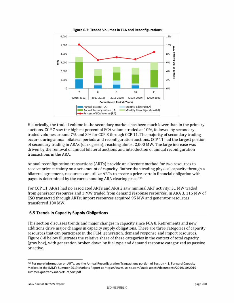
2020 Annual Markets Report page 200 ISO-NE PUBLIC
Figure 6-7: Traded Volumes in FCA and Reconfigurations
Historically, the traded volume in the secondary markets has been much lower than in the primary auctions. CCP 7 saw the highest percent of FCA volume traded at 10%, followed by secondary traded volumes around 7% and 8% for CCP 8 through CCP 11. The majority of secondary trading occurs during annual bilateral periods and reconfiguration auctions. CCP 11 had the largest portion of secondary trading in ARAs (dark green), reaching almost 2,000 MW. The large increase was driven by the removal of annual bilateral auctions and introduction of annual reconfiguration transactions in the ARA.
Annual reconfiguration transactions (ARTs) provide an alternate method for two resources to receive price certainty on a set amount of capacity. Rather than trading physical capacity through a bilateral agreement, resources can utilize ARTs to create a price-certain financial obligation with payouts determined by the corresponding ARA clearing price.259
For CCP 11, ARA1 had no associated ARTs and ARA 2 saw minimal ART activity; 31 MW traded from generator resources and 3 MW traded from demand response resources. In ARA 3, 115 MW of CSO transacted through ARTs; import resources acquired 95 MW and generator resources transferred 100 MW.
6.5 Trends in Capacity Supply Obligations
This section discusses trends and major changes in capacity since FCA 8. Retirements and new additions drive major changes in capacity supply obligations. There are three categories of capacity resources that can participate in the FCM: generation, demand response and import resources. Figure 6-8 below illustrates the relative share of these categories in the context of total capacity (gray box), with generation broken down by fuel type and demand response categorized as passive or active.
259 For more information on ARTs, see the Annual Reconfiguration Transactions portion of Section 4.1, Forward Capacity Market, in the IMM’s Summer 2019 Markets Report at https://www.iso-ne.com/static-assets/documents/2019/10/2019-summer-quarterly-markets-report.pdf
0%
2%
4%
6%
8%
10%
12%
0
1,000
2,000
3,000
4,000
5,000
6,000
7 8 9 10 11
(2016-2017) (2017-2018) (2018-2019) (2019-2020) (2020-2021)
Pe
rce
nt
of
FCA
Cle
are
d M
W
MW
Commitment Period (Years)
Annual Bilateral (LA) Monthly Bilateral (LA)Annual Reconfiguration (LA) Monthly Reconfiguration (LA)Percent of FCA Volume (RA)

2020 Annual Markets Report page 201 ISO-NE PUBLIC
Figure 6-8: Capacity Mix by Fuel Type from FCA 8 through FCA 15
Note: “Other” category includes landfill gas, methane, refuse, solar, steam, and wood.
The most substantial movements over the past eight FCAs were made by passive demand response resources and solar generation. Between FCAs 8 and 15 passive demand sharply increased from 1,961 MW to 3,213 MW, in line with state policy goals to increase energy efficiency. Solar capacity (located in the “Other” category) jumped from 5 MW in FCA 8 to 421 MW in FCA 15. More efficient solar technology drove down project costs and the renewable technology resource exemption helped solar projects enter the capacity market during FCAs 10-14.260 FCA 15 saw the largest integration of battery storage in the capacity mix. Since the first project cleared in FCA 13, battery storage projects have increased their share of capacity from 5 MW to 614 MW.
6.5.1 Retirement of Capacity Resources
A participant can choose to retire its resource by submitting a retirement request to the ISO.261 This is an irrevocable request to retire all or a portion of a resource.262 Up to FCA 11, this request was not contingent on market clearing prices; it was known as a non-price retirement. Starting in FCA 11, non-price retirements were replaced by priced-retirements which go through a cost-review process to establish if the bid may be an attempt to inflate clearing prices above competitive levels to the benefit of the remaining participant’s portfolio. A resource can also choose an unconditional retirement, choosing to retire regardless of the ISO’s reliability determination.
Retired generating resources with capacity exceeding 50 MW from FCA 8 are shown in Table 6-1 below.
260 The renewable technology resource (RTR) exemption was exhausted in FCA 15, allowing only 19 MW of qualified renewable capacity into the market during the auction.
261 FCA retirement permanently sheds a CSO; however, a resource may effectively retire before its FCA retirement, if it sheds its obligation through secondary markets and the retirement does not trigger reliability concerns.
262 Non-price retirement requests are subject to a review for reliability impacts. If the ISO notifies a resource owner of a reliability need for the resource, the resource owner has the option to retire the resource as requested or continue its operation until the reliability need has been met. Once the reliability need has been met, the resource must retire.
16,249 15,257 16,680 16,314 15,118 15,896 15,529 14,509
3,975 6,0536,109 6,554
6,589 5,298 4,988 5,705
4,0234,024
3,347 3,3443,343 3,339 3,333 3,326
3,0973,101 3,116 3,122
3,283 3,288 3,218 3,226
1,9612,156 2,369 2,791 2,975 3,355 3,327 3,213
33,712 34,695 35,567 35,835
34,828 34,839 33,956 34,621
0
5,000
10,000
15,000
20,000
25,000
30,000
35,000
40,000
45,000
8 9 10 11 12 13 14 15
(2017-2018) (2018-2019) (2019-2020) (2020-2021) (2021-2022) (2022-2023) (2023-2024) (2024-2025)
MW
Forward Capacity Auction (Years)
Gas Oil Nuclear Hydro Passive Import Other Coal Active Wind Battery Storage

2020 Annual Markets Report page 202 ISO-NE PUBLIC
Table 6-1: Generating Resource Retirements over 50 MW from FCA 8 to FCA 15
FCA # (Commitment Period)
Resource Name Fuel Type Capacity Zone FCA MW
FCA 8 (2017/18) Brayton Point 1 Coal SEMA 228
FCA 8 (2017/18) Brayton Point 2 Coal SEMA 226
FCA 8 (2017/18) Brayton Point 3 Coal SEMA 610
FCA 8 (2017/18) Brayton Point 4 Coal SEMA 422
FCA 8 (2017/18) Bridgeport Harbor 2 Oil Connecticut 130
FCA 8 (2017/18) Norwalk Harbor 1 Oil Connecticut 162
FCA 8 (2017/18) Norwalk Harbor 2 Oil Connecticut 168
FCA 8 (2017/18) Vermont Yankee Nuclear Nuclear Vermont 604
FCA 8 Total (resources > 50 MW) 2,550 MW
FCA 9 (2018/19) Mt. Tom. Coal WCMA 144
FCA 10 (2019/20) Pilgrim Nuclear Nuclear SEMA 677
FCA 12 (2021/22) Bridgeport Harbor 3 Oil Connecticut 383
FCA 13 (2022/23) Mystic 7 Oil NEMA/Boston 575
FCA 14 (2023/24) Yarmouth 1 Oil Maine 50
FCA 14 (2023/24) Yarmouth 2 Oil Maine 51
FCA 14 Total (resources > 50 MW) 101 MW
FCA 15 (2024/25) Mystic 9 Gas NEMA/Boston 710
FCA 15 (2024/25) Mystic 8 Gas NEMA/Boston 703
FCA 15 (2024/25) West Springfield 3 Gas WCMA 95
FCA 15 (2024/25) CDECCA Gas Connecticut 52
FCA 15 Total (resources > 50 MW) 1,560 MW
Note: The capacity defined here is the most recent non-zero FCA cleared capacity for each resource.
Energy policy and market dynamics have been cited as reasons leading to increased retirement pressure on nuclear, coal- and oil-fired generators. Increasing emissions prices and other energy polices have led to increased production costs. Many of the retiring resources are older resources that may require environmental upgrades or major overhauls. FCA 15 was the first auction in which older natural gas-fired generators began to retire. The retirement of older natural gas-fired generators is expected as the market shifts toward more efficient gas technology and large-scale renewable projects.
6.5.2 New Entry of Capacity Resources
This section provides an overview of major new resources entering the FCM. New entry typically implies a resource entering the market for the first time. However, existing resources that require significant investment to repower or provide incremental capacity, and meet the relevant dollar per kilowatt thresholds in the tariff, can also qualify as new capacity resources.263 Project sponsors of new capacity resources can elect to lock in the FCA clearing price for up to seven years.
263 See Market Rule 1, Section III.13.1

2020 Annual Markets Report page 203 ISO-NE PUBLIC
Newer, cleaner and more efficient technology, combined with low natural gas prices, increasing emissions costs, and environmental regulations have contributed to more investment in new natural gas-fired generators. Figure 6-9 represents new generation capacity by fuel type since FCA 8.
Figure 6-9: New Generation Capacity by Fuel Type from FCA 8 to FCA 15
Note: “Other” category includes landfill gas, methane, refuse, steam, and wood.
The majority of new additions between FCA 8 and FCA 13 were natural gas-fired resources. In FCA 9, over 1,000 MW of capacity was added; the largest addition was CPV Towantic, a 725 MW combined cycle resource in Connecticut. FCA 10 saw the largest amount of new generation entry, with an additional 1,400 MW of new natural gas-fired capacity. Three natural gas-fired resources accounted for 94% of this supply: Bridgeport Harbor 6 (484 MW), Canal 3 (333 MW), and Burrillville Energy Center (485 MW).264
For FCA 14, no new, large gas-fired resources cleared in the auction. Instead, an increase in state-sponsored solar resources and new wind resources were the primary sources of new cleared generation. Total new cleared solar capacity increased by 36%, from 141 MW in FCA 13, to 192 MW in FCA 14. The auction saw the last significant utilization of the renewable technology resource exemption, leaving only 19 MW of the exemption for FCA 15.
In FCA 15, new gas-fired capacity entered the market again, driven by a 334 MW repowering of Ocean State Power in Rhode Island. Battery storage projects qualified a significant portion of capacity into the market for the first time, clearing 596 MW of new capacity in the auction. Updated assumptions on battery storage project revenues reduced their minimum offer price, allowing these resources to offer below the low system clearing prices.
264 In September 2018, ISO-NE filed to terminate the 485 MW CSO of the Burrillville Energy Center, which was accepted by the Commission. Per the filing, the project sponsor had not made sufficient progress to achieve Clear River Unit 1’s critical path schedule milestones, and the commercial operation date for Clear River Unit 1 was more than two years beyond June 1, 2019, which was the start of the Capacity Commitment Period in which the resource first obtained a CSO.
$0
$2
$4
$6
$8
$10
$12
$14
$16
0
200
400
600
800
1,000
1,200
1,400
1,600
8 9 10 11 12 13 14 15
(2017-2018)
(2018-2019)
(2019-2020)
(2020-2021)
(2021-2022)
(2022-2023)
(2023-2024)
(2024-2025)
MW
FCA (Years)
Natural Gas Hydro Wind Solar Battery Storage Other
Right Axis: FCASystem-Wide Clearing Price ($/kW-month)

2020 Annual Markets Report page 204 ISO-NE PUBLIC
Significant increases in new passive demand response resources have more than offset active demand response retirements as with the previous FCA. Passive demand response is defined as on-peak and seasonal-peak resources. Active demand response is broken into real-time demand response and emergency generation.265 Figure 6-10 below shows cleared new active and passive resources since FCA 8.
Figure 6-10: New Demand (Reduction) Resources with a CSO
The annual additions of new demand resources in the FCM is primarily driven by state-sponsored energy efficiency programs that participate in the FCM as passive (on-peak or seasonal-peak) supply resources. FCA 13 saw the peak of new demand response capacity, with over 650 MW of new demand resources clearing in the auction. Since then, new demand response capacity has decreased, with only 170 MW clearing in FCA 15.
6.6 Market Competitiveness
This section discusses the competitiveness of the Forward Capacity Market (FCM) using two key metrics: the Residual Supply Index (RSI) and the Pivotal Supplier Test (PST).
The RSI measures the percent of capacity remaining in the market after removing the largest capacity supplier. The PST determines whether the ISO needs a supplier’s capacity to meet system and import-constrained zone requirements.266 Both metrics respect system constraints and account for affiliations between suppliers to reflect all capacity under a supplier’s control. These metrics
265 On-peak resources are energy efficiency and load-reducing distributed generation projects that provide long-term peak capacity reduction. Seasonal-peak resources are comprised of energy efficiency projects that also provide long-term peak reductions. The difference is that seasonal-peak resources provide reductions at or near the system peak, meaning they have a broader definition of peak hours. Lastly, real-time demand response resources are dispatchable resources that provide reliability during demand response events.
266 Section III.A.23 of the Tariff.
0
100
200
300
400
500
600
700
8 9 10 11 12 13 14 15
(2017-2018) (2018-2019) (2019-2020) (2020-2021) (2021-2022) (2022-2023) (2023-2024) (2024-2025)
MW
FCA (Years)
Passive Active

2020 Annual Markets Report page 205 ISO-NE PUBLIC
consider only existing resources prior to the auction to avoid predicting intra-auction new supply behavior.267
The RSI measures the percentage of capacity requirements (system or zonal) that can be met without capacity from the largest supplier’s portfolio of qualified capacity resources. It is measured on a continuous scale from zero to an uncapped upper limit. When the RSI is greater than 100%, suppliers other than the largest supplier have enough capacity to meet the relevant capacity requirement. This indicates that the largest supplier should have little opportunity to profitably increase the market-clearing price. Alternatively, if the RSI is less than 100%, the largest supplier is needed to meet demand. Consequently, the largest supplier could increase its offer prices above competitive levels to increase the market clearing price. Therefore, the lowest possible value of zero represents a pure monopoly scenario.
While the RSI uses a continuous measure and provides a sense of the largest supplier’s ability to influence clearing prices, the PST is binary and asks whether each individual supplier is needed to meet the system and import-constrained zone requirements. The PST therefore provides the total number of suppliers who may be able to influence prices. The PST compares (1) the total existing capacity in a zone without a given supplier’s portfolio of existing capacity to (2) the relevant capacity requirement for the zone.268 If the former quantity is less than the latter quantity, the supplier is pivotal. As a result, any de-list bids a pivotal supplier has submitted at prices above the dynamic de-list bid threshold may be subject to mitigation.269 This process ensures that suppliers do not withdraw capacity from the auction at uncompetitive prices to raise the FCA clearing price in a way that may benefit the remainder of their portfolio.
Both metrics use the following inputs:
Capacity requirements – both at the system level (Net Installed Capacity requirement, or Net ICR) and the import-constrained area level (Local Sourcing Requirement, or LSR). The Net ICR and LSR change from year to year.
Capacity zone modelling – different capacity zones are modelled for different FCAs depending on the quantity of capacity in the zone and transmission constraints.270
The total quantity of existing capacity – a value driven by retirements from existing resources and additions from new resources (which become existing resources in subsequent years). Recently, there have been steady gains in large new and incremental generation (described in Section 6.5.2).
Supplier-specific portfolios of existing capacity – values that can change year-over-year as a result of mergers, acquisitions, divestitures, affiliations, resource performance, etc. To avoid providing supplier-specific data, these are not described in any detail in this document, but should be taken into account when considering the analysis.
267 As defined in Section III.A.23.4 of the Tariff, for the purposes of this test, “the FCA Qualified Capacity of a supplier includes the capacity of Existing Generating Capacity Resources, Existing Demand Resources, Existing Import Capacity Resources, and New Import Capacity Resources (other than (i) a New Import Capacity Resource that is backed by a single new External Resource and that is associated with an investment in transmission that increases New England’s import capability; and (ii) a New Import Capacity Resource associated with an Elective Transmission Upgrade).”
268 The relevant requirements are the Net ICR (Installed Capacity Requirement net of Hydro-Quebec Interconnection Capability Credits) at the system level and the Local Sourcing Requirement (LSR) at the import-constrained zonal level.
269 Note that there are certain conditions under which capacity is treated as non-pivotal. These conditions are described in Section III.A.23.2 of the Tariff.

2020 Annual Markets Report page 206 ISO-NE PUBLIC
Residual Supply Index Results
The RSIs for the system and for SENE (the only import-constrained zone during the reporting period) over the past five FCAs are illustrated in Figure 6-11 below.271
Figure 6-11: Capacity Market Residual Supply Index, by FCA and Zone
The RSI was below 100% in every auction since FCA 11 at both the system and zonal levels, except for FCA 14. An RSI below 100% indicates the presence of at least one pivotal supplier. The system-wide RSI (yellow) increased from 96% in FCA 11 to a high of 103% in FCA 14, decreasing slightly to 98% in FCA 15. The changes can be attributed to a variety of factors including: changes to the largest supplier (there were two over the study period caused by resource retirements, acquisitions, and sales), the steady procurement of new generation in recent FCAs, and reductions in Net ICR.
The zonal RSI (red) increased from 80% in FCA 10 to a high of 93% in FCAs 12 and 14, decreasing to 79% in FCA 15. The decrease in FCA 13 was due to a higher LSR value and retirements within the capacity zone.
Pivotal Supplier Test Results
The number of suppliers, some of which were pivotal, within each zone over the past five FCAs are presented in Figure 6-12 below. To provide additional insight into the approximate portfolio size needed to be pivotal, the figure also presents the margin by which the capacity exceeded or fell below the relevant capacity requirement. For example, consider the SENE capacity zone in FCA 14. The amount of existing capacity exceeded the LSR, resulting in a capacity margin of approximately 1,105 MW (right axis – blue marker). Consequently, only suppliers with a portfolio of greater than
271The RSI measure in this section leverages the capacity counting rules outlined in the Tariff for the Pivotal Supplier Test. These are the most recent capacity counting rules for this purpose and were in effect beginning with FCA 10. They are used for prior auctions periods for consistency.

2020 Annual Markets Report page 207 ISO-NE PUBLIC
1,105 MW in this zone were pivotal in FCA 14. Of the 53 suppliers in SENE in FCA 14 (left axis – yellow bar), only four (highlighted in yellow) were pivotal.
Figure 6-12: Overview of Suppliers, Pivotal Supplier, and Capacity Margin, by Zone
Now consider the SENE capacity zone in FCA 15. The amount of existing capacity was less than the LSR, resulting in a capacity margin of approximately -711 MW. The negative capacity margin means, given the existing quantity of supply in SENE, there was not enough supply to meet the LSR prior to FCA 15. Consequently, every supplier located in SENE of every portfolio size was pivotal because, even with every supplier present, the zone still fell short of the LSR. Note that, despite the negative margin in SENE, the FCA 15 system-wide margin was approximately 1,922 MW with no pivotal suppliers
At the system level, the capacity margin remained high over the past five FCAs. In FCA 14, a significant increase in the margin resulted in a supplier needing a portfolio of over 3,650 MW to be pivotal, resulting in no pivotal suppliers. The increase in the system capacity margin from 1,650 MW in FCA 13 to over 3,650 MW in FCA 14 was driven largely by a significant decrease in net ICR, down 1,260 MW from FCA 13 to FCA 14. The capacity margin decreased significantly in FCA 15, to approximately 1,922 MW. The decrease in the margin in FCA 15 was also driven by a significant increase in net ICR, from 32,490 MW in FCA 14 to 33,270 MW in FCA 15 (an increase of 780 MW). The exit of the Mystic 8 & 9 generators from the supply stack also contributed to the decreased margin in FCA 15. Despite the decreased margin in FCA 15, there have still been few pivotal suppliers at the system level since FCA 11.
The SENE capacity zone margin rose in FCA 14 primarily due to a significant drop in the LSR from the prior year, and fell dramatically in FCA 15 due to a combination of an increase in the LSR and a decrease in zonal supply caused by the retirement of the 1,413 MW Mystic generators. The margin fell approximately 1,800 MW, from 1,100 MW in FCA 14 to -711 MW in FCA 15. The capacity deficit led to all 58 suppliers in SENE being pivotal in FCA 15, up from four pivotal suppliers in FCA 14.
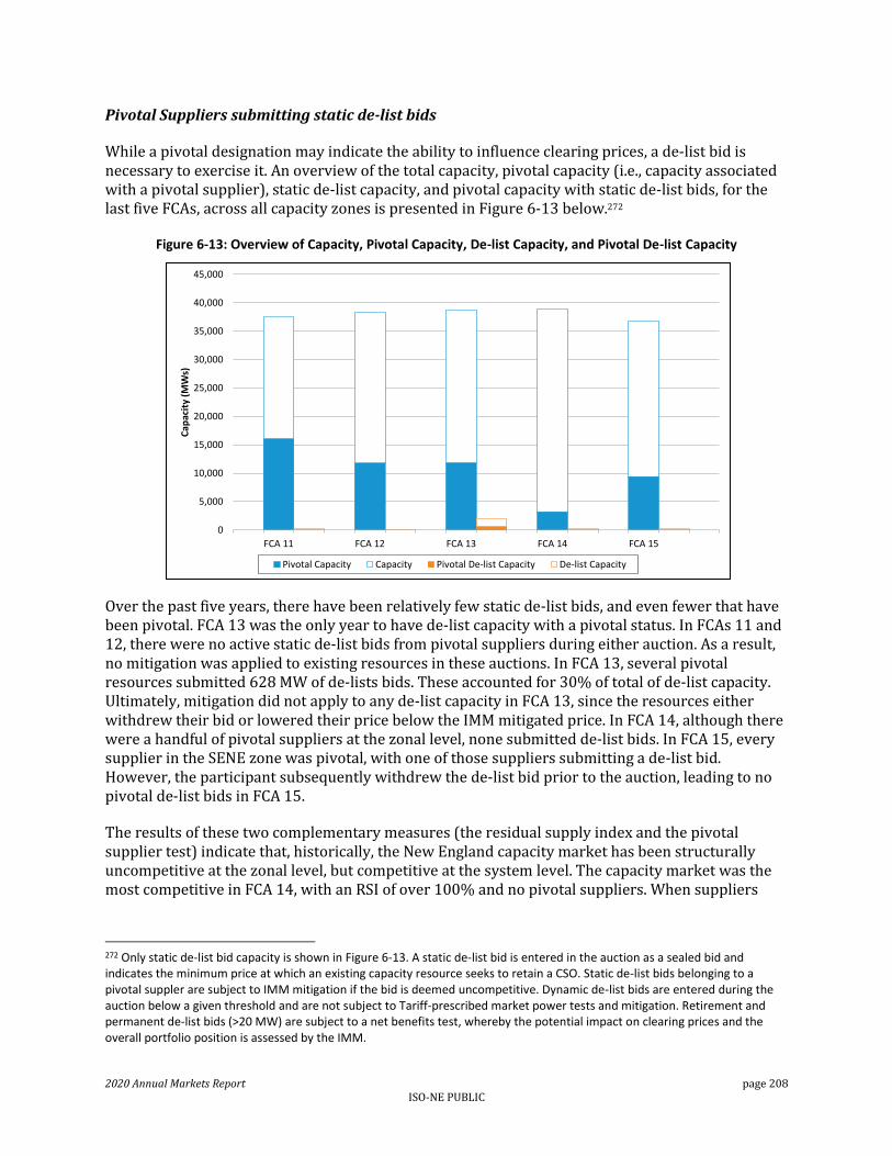
2020 Annual Markets Report page 208 ISO-NE PUBLIC
Pivotal Suppliers submitting static de-list bids
While a pivotal designation may indicate the ability to influence clearing prices, a de-list bid is necessary to exercise it. An overview of the total capacity, pivotal capacity (i.e., capacity associated with a pivotal supplier), static de-list capacity, and pivotal capacity with static de-list bids, for the last five FCAs, across all capacity zones is presented in Figure 6-13 below.272
Figure 6-13: Overview of Capacity, Pivotal Capacity, De-list Capacity, and Pivotal De-list Capacity
Over the past five years, there have been relatively few static de-list bids, and even fewer that have been pivotal. FCA 13 was the only year to have de-list capacity with a pivotal status. In FCAs 11 and 12, there were no active static de-list bids from pivotal suppliers during either auction. As a result, no mitigation was applied to existing resources in these auctions. In FCA 13, several pivotal resources submitted 628 MW of de-lists bids. These accounted for 30% of total of de-list capacity. Ultimately, mitigation did not apply to any de-list capacity in FCA 13, since the resources either withdrew their bid or lowered their price below the IMM mitigated price. In FCA 14, although there were a handful of pivotal suppliers at the zonal level, none submitted de-list bids. In FCA 15, every supplier in the SENE zone was pivotal, with one of those suppliers submitting a de-list bid. However, the participant subsequently withdrew the de-list bid prior to the auction, leading to no pivotal de-list bids in FCA 15.
The results of these two complementary measures (the residual supply index and the pivotal supplier test) indicate that, historically, the New England capacity market has been structurally uncompetitive at the zonal level, but competitive at the system level. The capacity market was the most competitive in FCA 14, with an RSI of over 100% and no pivotal suppliers. When suppliers
272 Only static de-list bid capacity is shown in Figure 6-13. A static de-list bid is entered in the auction as a sealed bid and indicates the minimum price at which an existing capacity resource seeks to retain a CSO. Static de-list bids belonging to a pivotal suppler are subject to IMM mitigation if the bid is deemed uncompetitive. Dynamic de-list bids are entered during the auction below a given threshold and are not subject to Tariff-prescribed market power tests and mitigation. Retirement and permanent de-list bids (>20 MW) are subject to a net benefits test, whereby the potential impact on clearing prices and the overall portfolio position is assessed by the IMM.
0
5,000
10,000
15,000
20,000
25,000
30,000
35,000
40,000
45,000
FCA 11 FCA 12 FCA 13 FCA 14 FCA 15
Cap
acit
y (M
Ws)
Pivotal Capacity Capacity Pivotal De-list Capacity De-list Capacity

2020 Annual Markets Report page 209 ISO-NE PUBLIC
have market power, buyer- and supplier-side mitigation rules are in place to prevent the potential exercise of market power. This is discussed in the next section.
6.7 Capacity Market Mitigation
In this section, we provide an overview of the mitigation measures employed in the FCM, as well as summary statistics on the number and impact of these measures. This section presents summary information for FCA 11 through FCA 15.
Two forms of mitigation apply to FCA bids and offers: supplier-side mitigation for existing resources and buyer-side mitigation, namely the Minimum Offer Price Rules (MOPR) for new resources.
6.7.1 Supplier-Side Market Power
A market participant attempting to exercise supplier-side market power will try to economically withhold capacity during the FCA – for a single year or permanently - in an effort to increase the clearing price above a competitive level. An inflated clearing price can benefit the remaining resources in the market participant’s portfolio, as well as the portfolios of other suppliers. A market participant would only attempt this if they believed (1) their actions would inflate the clearing price and (2) the revenue gain from their remaining portfolio would more than offset the revenue loss from the withheld capacity.
De-list bids are the mechanism that allow capacity resources to remove some or all of their capacity from the market for one or more commitment periods. De-list bids specify the lowest price that a resource would be willing to accept in order to take on a capacity supply obligation (CSO). To restrict resources from leaving the market at a price greater than their competitive offers, the IMM reviews de-list bids above a proxy competitive offer threshold called the dynamic de-list threshold (DDBT) price.273 A competitive de-list bid is consistent with the market participant’s net going forward costs, expected capacity performance payments, risk premium, and opportunity costs. All existing capacity resources, as well as certain types of new import capacity resources (described below), are subject to the pivotal supplier test, which is described in more detail in the last section. If the IMM determines that a de-list bid is uncompetitive and the supplier fails the pivotal supplier test, the IMM mitigates the de-list bid to a competitive price.
While there are a variety of de-list bid types, only a few require review by the IMM. Prior to FCA 11, reviewable de-list bid types included: general static de-list bids, import and export bids, and permanent de-list bids. 274,275
273 De-list bids priced below the DDBT are presumed to be competitive and are not subject to the IMM’s cost review or mitigation; consequently, they are not discussed in this section. Market participants can dynamically de-list resources if the auction price falls below the DDBT price. The DDBT has undergone a number of revisions since the start of the FCM. The DDBT price was $5.50/kW-month in FCAs 11 and 12, and $4.30/kW-month in FCAs 13, 14 and 15.
274 In FCA 10, various changes were made, including limiting this review to new import capacity resources without transmission investments.
275 The term “general” is used to differentiate between other types of static de-list bids, including ambient air static de-list bids and ISO low winter static de-list bids, which are not subject to IMM review.

2020 Annual Markets Report page 210 ISO-NE PUBLIC
Retirement and permanent de-list bids
In FCA 11, permanent de-list bids were replaced by “retirement and permanent de-list bids” for resources greater than 20 MW. Between FCAs 8 and 11, there were no permanent de-list bids or retirement de-list bids for resources greater than 20 MW, and there was only one export de-list bid. In FCA 12, the lead participant for Bridgeport Harbor 3 submitted a 383 MW retirement de-list bid, and Enerwise Global Technologies, Inc. submitted retirement de-list bids for over 100 MWs of capacity. In FCA 13, over 1,400 MW of retirement de-list bids came from Mystic 8 and 9. While their bids were mitigated down, they were denied for reliability and treated as existing capacity in FCAs 13 and 14. In FCA 15, the Mystic generators were no longer retained and two more significant retirements occurred (CDECCA and West Springfield 3), combining for a total of 1,560 MW.
Static de-list bids
For FCA 11 through FCA 15, the IMM reviewed 83 general static de-list bids from 13 different lead participants, totaling roughly 8,700 MW of capacity (an average of 1,700 MW per auction).276 Generation resources accounted for 8,400 MW of the total capacity, even though they only accounted for 46 of the 83 general static de-list bid submissions. Two import resources made up 1 MW of total capacity and 35 demand response resources made up 300 MW of the total capacity; both resource types consistently have smaller-sized projects than generating resources. Separate from the above statistics, the IMM reviewed supply offers from import capacity resources without transmission investments, totaling approximately 1,700 MW.277
As previously stated, the IMM reviews de-list bid submissions to determine if they are consistent with the participant’s net going forward costs, expected capacity performance payments, risk premium, and opportunity costs. This process resulted in mitigations for approximately 37% of the general static de-list bids (93% of de-list MW capacity) from FCA 11 to FCA 15.278
Summary statistics for static de-list bids from FCA 11 through FCA 15 as well as the path the bids took from the time of initial submittal to the auction are provided in Figure 6-14 below. Note that all de-list bid prices are megawatt-weighted averages.279
276 A resource with a static de-list bid in each of the three auctions would be counted three times in the MW total; however, the associated lead participant is only counted once.
277 For market power mitigation purposes, import resources without transmission investment are evaluated for seller-side market power. New imports resources with associated transmission investment are evaluated under the MOPR.
278 If a supplier is pivotal, the IMM-determined value is entered into the auction; if not, the participant-submitted bid is entered. The mitigation only takes effect if the supplier is deemed pivotal, an evaluation that is done some months after the cost review process in completed. 279 Price calculations are not presented for new import capacity resources because, depending on the circumstances, the direction of the price difference can vary for price-quantity pairs within the same supply offer. Consequently, the resulting price difference summary statistics are less meaningful.

2020 Annual Markets Report page 211 ISO-NE PUBLIC
Figure 6-14: General Static De-list Bid Summary Statistics, by Key Milestone Action (FCAs 11 – 15) 280
Roughly 63% of bids were accepted by the IMM without any changes (left box, second level). Of the static de-list bids that were denied, many were voluntarily withdrawn or the bid price further reduced prior to the auction. For resources that were denied and went to the auction (box furthest to the right, third level), the weighted-average price of denied static de-list bids was $7.11/kW-month less than the market participant’s originally submitted price.
As discussed above, only de-list bids belonging to pivotal suppliers are mitigated. There were active de-list bids from pivotal suppliers in FCA 13 only; the four other auctions did not have any de-list bids from pivotal suppliers, none of which were mitigated. In FCA 13, the denied de-list bids for three resources (628 MW) were mitigated in the auction.
6.7.2 Test Price Review
The test price mitigation rule was introduced in FCA 14, and applies to resources (above 3 MW) seeking to retire through the substitution auction. The rule is designed to protect the primary FCA from price suppression, by mitigating behavior commonly referred to as “bid shading”.
Bid shading occurs when an existing resource may have an incentive to include the value of a severance payment in its primary auction bid price. This behavior would increase the likelihood of retaining its CSO, and subsequently trading out of it for a severance payment in the substitution auction. This could have a price-suppressing impact in the FCA. The test price is an IMM-calculated value, based on a cost submission from the resource owner, which represents the competitive cost of obtaining a CSO, excluding any expected severance payment from the substitution auction.
The test price serves as a screen to determine whether a resource’s demand bid will be entered into the substitution auction based on the clearing price of the primary auction. If the resource’s test price is below the primary auction clearing price, the resource is allowed to enter the substitution
280 All MW values are rounded to the nearest hundred.
83 Static De-list Bids8,700 MW
$8.84/kW-mon
Accepted
52 Static De-list Bids600 MW
Submitted: $12.25/kW-mon
Reduced: $12.10/kW-mon
Denied
Submitted
26 Static De-list Bids7,500 MW
Submitted: $8.24/kW-mon
IMM-Determined: $5.49/kW-mon
5 Static De-list Bids600 MW
Submitted: $12.63/kW-mon
IMM-Determined: $5.27/kW-mon
Withdrawn Static De-List Bid (to auction without static-delist)
To Auction
Withdrawn Static De-List Bid (to auction without static-delist)
To Auction with Static De-List Bid To Auction with Static De-List Bid
31 Static De-list Bids8,000 MW
Submitted: $8.55/kW-mon
IMM-Determined: $5.47/kW-mon
49 Static De-list Bids600 MW
Submitted: $12.32/kW-mon
3 Static De-list Bids10 MW
Submitted: $7.88/kW-mon

2020 Annual Markets Report page 212 ISO-NE PUBLIC
auction. If the test price is greater than the primary auction clearing price, the resource is not permitted to enter a demand bid into the substitution auction.
In FCA 15, thirteen existing resources with a combined capacity of 196 MW elected to participate in the substitution auction. The weighted-average submitted test price was $11.28/kW-mo. The IMM reviewed 5 and denied 3 resources (above the 3 MW threshold), with a combined capacity of 188 MW. The weighted-average IMM-determined test price was $10.82/kW-mo. Regardless of test price mitigation no resource retained a CSO that they could trade out of in the substitution auction. The clearing price in FCA 15 fell well below all the IMM–determined test prices and indeed below all submitted test prices. Therefore, the mitigation of submitted test prices did not have an impact on demand side participation in the substitution auction.
6.7.3 Minimum Offer Price Rule
A market participant attempting to exercise buyer-side market power will try to offer capacity below cost in an effort to decrease the clearing price. A depressed clearing price benefits capacity buyers, not necessarily capacity suppliers. In practice, the risk of price suppression in the ISO-NE market is largely due to out-of-market revenue streams to incent new build to help meet the states’ environmental goals, as opposed to the intentional exercise of market power. To guard against price suppression, the IMM evaluates requests to offer capacity below pre-determined competitive threshold prices, or Offer Review Trigger Prices (ORTPs). Market participants that want to offer below the relevant ORTP must submit detailed financial information to the IMM about their proposed project. The financial information is reviewed for out-of-market revenues or other payments that would allow the market participant to offer capacity below cost.281 The out-of-market revenues are either replaced with market-based revenues or removed entirely and the offer is recalculated to a higher, competitive price (i.e. the offer is mitigated).
For FCAs 11 through 15, the IMM reviewed nearly 490 new supply offers282 from participants requesting to offer below the ORTP.283 These offers came from 64 different lead participants and totaled 16,400 MWs of qualified capacity, of which about 13,000 MW (~79%) entered the auction.284 Generation resources accounted for the majority of new capacity reviewed, with 91% of the total (13,300 MW). Demand response resources accounted for the remaining 9% (1,400 MW). No new import capacity resources with transmission investments completed the review process.
Summary statistics for resources requesting to offer below their respective ORTP in FCAs 11 through 15 are provided in Figure 6-15 below. Note that all offer prices are megawatt-weighted averages.
281 Out-of-market revenues are defined in Section III.A.21.2 of the tariff.
282 Note that the count does not capture all unique resources. If a resource was mitigated in FCA 11 and did not clear, it could return in FCA 12 and would be captured twice in the count.
283 Note that this total does not include supply offers from new import capacity resources without transmission investments, which are discussed in the supplier-side market power section.
284 A resource with a new supply offer in each of the three auctions would be counted three times in the MW total. In addition, where FCA qualified capacity does not exist for a resource (e.g., the proposal was withdrawn or denied), the summer capacity from the resource’s show of interest is used instead. Consequently, the presented total overstates the actual capacity.

2020 Annual Markets Report page 213 ISO-NE PUBLIC
Figure 6-15: Reviewable Offer Request Summary Statistics, by Key Milestone Action (FCAs 11 – 15)285
The IMM mitigated approximately 70% (341) of new supply offers it reviewed, or approximately 74% (10,800 MW) of new supply capacity.286 Similar to supplier-side mitigation, the degree of MOPR mitigation can be measured by the relative increase in the offer floor price imposed by the IMM. The mitigation process (box furthest to the right, second level) resulted in an average increase in offer price of $2.45/kW-month (from a submitted price of $2.36/kW-month to an IMM-determined price of $4.81/kW-month).
285 All MW values are rounded to the nearest hundred.
286 Note that the value does not capture not all unique capacity. In other words, if a 100 MW PV resource was mitigated in FCA 11 and did not clear, it could return in FCA 12 and would be captured as 200 MW
484 New Supply Offers14,700 MW
$2.48/kW-mon
Accepted
143 New Supply Offers3,800 MW
$2.98/kW-mon
Denied
Submitted
76 New Supply Offers3,100 MW
Submitted: $2.15/kW-mon
IMM-Determined: $6.96/kW-mon
Withdrawn To Auction
265 New Supply Offers7,800 MW
Submitted: $2.36/kW-mon
IMM-Determined: $4.81/kW-mon
17 New Supply Offers300 MW
$1.82/kW-mon
126 New Supply Offers3,500 MW
$3.09/kW-mon
Withdrawn To Auction
341 New Supply Offers10,800 MW
Submitted: $2.30/kW-mon
IMM-Determined: $5.42/kW-mon

2020 Annual Markets Report page 214 ISO-NE PUBLIC
Section 7 Ancillary Services
This section reviews the performance of ancillary services in ISO New England’s forward and real-time markets. There are six main types of ancillary service products:
Real-time operating reserves represent additional generating capacity that is available to respond to unexpected contingencies (such as the unexpected loss of a generator or transmission line) during operation of the real-time energy market.
Forward reserves represent the procurement of fast-response reserve capability from generators in advance of the delivery period; that is, the ability to start and ramp quickly in the event of system contingencies.
Regulation service is provided by generators that alter their energy output over very short time intervals (minute-to-minute) to balance supply and demand in the real-time energy market.
The Winter Reliability Program was implemented by the ISO from 2013 to 2018 to remedy fuel supply issues that threatened reliability. The program paid market participants to purchase sufficient fuel inventories (oil or LNG) or provide additional demand response during the winter months, when it is more challenging to procure natural gas. The program ended after Winter 2018, coinciding with the start of the pay-for-performance rules in the capacity market in June 2018.
Voltage support helps the ISO maintain an acceptable range of voltage on the transmission system, and is necessary for the reliable flow of electricity. The ISO regulates voltage through reactive power dispatch, and the generators that provide this service receive voltage support payments.
Blackstart service is provided by generators that are able to restart quickly without outside electrical supply The ISO selects and compensates strategically located generators for providing blackstart service. This service is necessary to facilitate power system restoration in the event of a partial or complete system shutdown.
Ancillary service costs by submarket are shown in Figure 7-1 below.

2020 Annual Markets Report page 215 ISO-NE PUBLIC
Figure 7-1: Ancillary Service Costs by Product (in $ millions)287
In 2020, the costs of most ancillary service products and their associated make-whole payments were lower than or similar to 2019 costs. Overall, ancillary costs declined to $103 million in 2020 from $114 million in 2019, and were at their lowest total over the five-year reporting period. The only category with a notable increase was blackstart costs, which rose by $7.8 million or 37% in 2020. The increase was due to blackstart fleet composition changes, coupled with a rate structure change. There were no Winter Reliability Program payments in 2020 or 2019 because the program expired in March 2018.
7.1 Real-Time Operating Reserves
Bulk power systems need reserve capacity to be able to respond to contingencies, such as the unexpected loss of a large generator or transmission line. To ensure that adequate reserves are available, the ISO procures several different reserve products through the locational Forward Reserve Market (FRM) and the real-time co-optimized energy and reserves market. The following section reviews real-time operating reserve products and analyzes real-time reserve outcomes in 2020.
7.1.1 Real-Time Operating Reserve and Pricing Mechanics
There are four types of reserve products that can be provided by generators, dispatchable asset related demand, and demand response resources:
Ten-minute spinning reserve (TMSR): TMSR is the highest-quality reserve product. It is provided by online resources that can convert reserves to energy within 10 minutes. For example, a synchronized generator that can increase its output within 10 minutes can provide TMSR. This gives the system a high degree of certainty that it can recover from a significant system contingency quickly.
287 The Voltage Service category includes payments for capacity costs, lost opportunity costs, costs of energy consumed, and costs of energy produced.

2020 Annual Markets Report page 216 ISO-NE PUBLIC
Ten-minute non-spinning reserve (TMNSR): TMNSR is the second-highest quality reserve product. It is provided by offline resources that require a successful startup (e.g., a generator that can electrically synchronize to the grid and increase output within 10 minutes).
Thirty-minute operating reserve (TMOR): TMOR is a lower quality reserve product provided by less-flexible resources (e.g., an on-line resource that can increase output within 30 minutes or off-line resource that can electrically synchronize to the system and increase output within 30 minutes).
Local Thirty-minute operating reserve (Local TMOR): Local TMOR is thirty-minute operating reserve provided for a local reserve zone in order to meet the local second contingency in import-constrained areas. Local TMOR requirements are set for each of the local reserve zones: Connecticut (CT), Southwest Connecticut (SWCT), and NEMA/Boston.
Real-time prices for each of the above reserve products are determined by the ISO dispatch and pricing software. The software co-optimizes energy and reserves. That is, it solves for the least-cost dispatch, while meeting energy demand and satisfying the reserve requirements (see Section 2.2.5 for information on reserve requirements), and creates energy and reserve prices. A reserve price above zero occurs when the software must re-dispatch resources to satisfy the reserve requirement, which imposes additional costs to the system. When this happens, the reserve price is set by the resource with the highest re-dispatch cost (or opportunity cost) to provide the reserves, but is capped by the Reserve Constraint Penalty Factor (RCPF).
The software will not re-dispatch resources to meet reserves at any price. When the re-dispatch costs exceed the RCPF, the price will be set equal to the RCPF and the market software will not continue re-dispatching resources to meet reserves. RCPFs limit the re-dispatch cost the system will incur to satisfy reserve requirements. 288 These RCPFs are then reflected in the energy price due to the interdependence in procurement. The RCPFs also serve as a pricing mechanism that signals scarcity in real-time through high reserve prices. Each reserve product has a corresponding RCPF, as shown in Table 7-1 below.
Table 7-1: Reserve Constraint Penalty Factors
Requirement Requirement Sub-Category RCPF
($/MWh)
System TMSR (10-min spinning) 50
System TMNSR (10-min non-spinning) 1,500
System TMOR (30-min) Minimum TMOR 1,000
System TMOR (30-min) Replacement Reserves 250
Local TMOR 250
Although the TMSR is the highest-quality reserve product, it has the lowest RCPF ($50). On average, the cost incurred to re-dispatch resources providing TMSR is lower than the cost incurred to re-dispatch less flexible resources to provide 30-minute operating reserves. This is because there are
288 When an RCPF is reached and the real-time energy market’s optimization software stops re-dispatching resources to satisfy the reserve requirement, the ISO will manually re-dispatch resources to obtain the needed reserves, if possible.

2020 Annual Markets Report page 217 ISO-NE PUBLIC
additional costs associated with offline resources that are not already online and operating in merit like those providing TMSR. This is why the RCPFs associated with TMSR are less than the TMNSR and TMOR RCPFs; RCPFs are designed to reflect the upper range of the re-dispatch costs rather than the quality or value of the product.
To ensure that the incentives for providing the individual reserve products are correct, the market’s reserve prices maintain an ordinal ranking. This ranking is consistent with the quality of the reserves provided as follows:
10-Minute Spinning (TMSR) ≥ 10-Minute Non-Spinning (TMNSR) ≥ 30-Minute (TMOR)
The price of higher-quality reserve products must be at least as high as the price of lower-quality reserve products. For example, if the ISO alters the dispatch to provide TMOR at a cost of $40/MWh, the prices for TMSR and TMNSR both must be equal to or greater than $40/MWh. The ordinal ranking of reserve prices is also maintained when the ISO needs to re-dispatch the system to create multiple reserve products. For example, if the ISO re-dispatches the system to create TMSR, the reserve price is capped at $50/MWh, the TMSR RCPF. However, if the ISO re-dispatches the system to create TMSR and TMNSR, the reserve price is capped at $1,500/MWh for TMNSR resources and the higher-valued TMSR resources are paid $1,550/MWh – the sum of the two reserve products’ RCPFs – thereby preserving the ordinal ranking of the reserve product prices.
7.1.2 Real-Time Operating Reserve Payments
The payments presented in Figure 7-2 below are a measure of the value of real-time reserves between 2016 and 2020. The height of each bar represents the payments by system and local reserve products. Each bar comprises the product of aggregated resource real-time reserve designations and the reserve market clearing prices. The black diamond displays total net real-time reserve credits. The diamond will be lower than the height of the bars when real-time payments are “clawed back” to ensure resources paid in the forward reserve market are not paid again in the real-time reserve market.
Figure 7-2: Real-Time Reserve Payments 2016-2020
$0
$5
$10
$15
$20
$25
$30
$35
$40
2016 2017 2018 2019 2020
$ m
illio
ns
TMSR TMNSR TMOR
NEMA/Boston TMOR CT TMOR SWCT TMOR
Net RT Reserve Payments
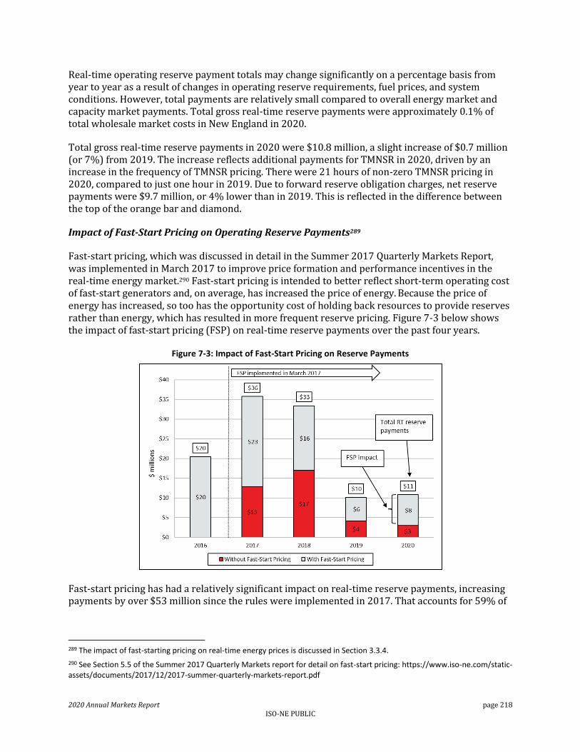
2020 Annual Markets Report page 218 ISO-NE PUBLIC
Real-time operating reserve payment totals may change significantly on a percentage basis from year to year as a result of changes in operating reserve requirements, fuel prices, and system conditions. However, total payments are relatively small compared to overall energy market and capacity market payments. Total gross real-time reserve payments were approximately 0.1% of total wholesale market costs in New England in 2020.
Total gross real-time reserve payments in 2020 were $10.8 million, a slight increase of $0.7 million (or 7%) from 2019. The increase reflects additional payments for TMNSR in 2020, driven by an increase in the frequency of TMNSR pricing. There were 21 hours of non-zero TMNSR pricing in 2020, compared to just one hour in 2019. Due to forward reserve obligation charges, net reserve payments were $9.7 million, or 4% lower than in 2019. This is reflected in the difference between the top of the orange bar and diamond.
Impact of Fast-Start Pricing on Operating Reserve Payments289
Fast-start pricing, which was discussed in detail in the Summer 2017 Quarterly Markets Report, was implemented in March 2017 to improve price formation and performance incentives in the real-time energy market.290 Fast-start pricing is intended to better reflect short-term operating cost of fast-start generators and, on average, has increased the price of energy. Because the price of energy has increased, so too has the opportunity cost of holding back resources to provide reserves rather than energy, which has resulted in more frequent reserve pricing. Figure 7-3 below shows the impact of fast-start pricing (FSP) on real-time reserve payments over the past four years.
Figure 7-3: Impact of Fast-Start Pricing on Reserve Payments
Fast-start pricing has had a relatively significant impact on real-time reserve payments, increasing payments by over $53 million since the rules were implemented in 2017. That accounts for 59% of
289 The impact of fast-starting pricing on real-time energy prices is discussed in Section 3.3.4.
290 See Section 5.5 of the Summer 2017 Quarterly Markets report for detail on fast-start pricing: https://www.iso-ne.com/static-assets/documents/2017/12/2017-summer-quarterly-markets-report.pdf

2020 Annual Markets Report page 219 ISO-NE PUBLIC
the $90 million in total payments since 2017. Without fast-start pricing, real-time reserve payments would have been approximately $3 million in 2020, compared to the actual amount of $11 million.
7.1.3 Real-Time Operating Reserve Prices: Frequency and Magnitude
Average reserve prices are a function of two factors: frequency and magnitude. Frequency represents how often (i.e., percentage of the time) a reserve product has a positive price (a price above $0/MWh). Magnitude is the average real-time reserve price for only the intervals where reserve prices were positive (non-zero). Figure 7-4 below illustrates both the frequency (left panel) and magnitude (right panel) of non-zero reserve prices by reserve product over time.
Figure 7-4: Frequency and Average of Non-Zero Reserve Prices
Figure 7-4 shows that the TMSR price was non-zero (i.e., above $0/MWh) for about 21% of all hours in 2020, up 4% from 2019. For those hours in which the TMSR price was positive, it averaged $7/MWh, a decrease from an average of $11/MWh in 2019 (right panel of Figure 7-4). The low non-zero TMSR price was driven by lower energy prices in 2020. The increase in frequency only partially offset the decline in average TMSR pricing, which is why TMSR payments were lower in 2020.
The frequency of non-zero TMNSR in positive pricing intervals increased from one hour in 2019 up to 21 hours in 2020. However, this was still small as a percentage of total hours (0.2%), which is why the increase isn’t noticeable on the left panel of Figure 7-4. The average price in positive TMNSR intervals dropped from $92/MWh in 2019 to $61/MWh in 2020. The low TMNSR magnitude and prices were driven by low energy prices and a lack of system events in 2020. Similarly, the frequency of positive pricing for system-wide TMOR increased to eight hours in 2020, up from no intervals in 2019. The presence of TMOR pricing ($86/MWh on average) led to an increase compared to 2019, but was much less than 2018 ($216/MWh on average). In 2020, there was no price separation among TMOR products, which indicates no local TMOR pricing. We can evaluate the impact of both frequency and magnitude by looking at real-time reserve prices for all pricing intervals in Figure 7-5 below.

2020 Annual Markets Report page 220 ISO-NE PUBLIC
Figure 7-5: Average Real-Time Reserve Prices for all Pricing Intervals
Average TMSR prices during all pricing intervals (i.e. zero- and non-zero pricing intervals) decreased by 17%, while TMNSR and TMOR slightly increased in 2020 relative to 2019. As shown in Figure 7-4, lower TMSR clearing prices partially offset a slight increase in TMSR frequency. Still, average prices for all intervals declined, which is reflected in lower TMSR payments discussed in Section 7.1.2. TMNSR and TMOR pricing increased from 2019 because there were more hours with pricing for those products. Average prices over all intervals were still less than $0.15/MWh in 2020.
Reserve Constraint Penalty Factors
RCPFs for reserve products are triggered due to either a shortage of available capacity to meet the reserve requirements or re-dispatch costs that exceed RCPF values. The number of five-minute intervals during which the RCPFs were triggered for each reserve constraint are shown in Figure 7-6 below.
Figure 7-6: Reserve Constraint Penalty Factor Activation Frequency
$0.00
$0.50
$1.00
$1.50
$2.00
$2.50
$3.00
$3.50
2016 2017 2018 2019 2020
$/M
Wh
TMSR TMNSR SWCT TMOR CT TMOR NEMA/Boston TMOR TMOR
NEMA/Boston, CT, and SWCTTMOR underneath TMOR
0.00%
0.20%
0.40%
0.60%
0.80%
1.00%
TMSR TMNSR TMOR NEMA/BostonTMOR
SWCT TMOR CT TMOR
% o
f R
CP
F ac
tiva
tio
n f
or
all i
nte
rval
s
2016 2017 2018 2019 2020

2020 Annual Markets Report page 221 ISO-NE PUBLIC
In 2020, only the RCPF for the TMSR product bound, with a frequency of 173 five-minute intervals (0.2% of total intervals), or about 14 hours over the year; this was the lowest frequency in the reporting period. The TMSR RCPF had the highest frequency of activations due to the higher frequency of non-zero TMSR pricing intervals and its relatively low RCPF value ($50/MWh) compared to the other products. This means the dispatch software will stop trying to re-dispatch the system for TMSR much sooner than for the other reserve products with significantly higher RCPF values.
When RCPFs are triggered due to a reserve shortage, the reserve price directly impacts the energy price. During these times, the RCPF value is added to the energy price because satisfying any additional increment of load will decrease the amount of available system reserves by the same amount. The RCPF value determines the price of reserves during scarcity events. Thus, the LMP will reflect the total cost of serving an additional increment of load including the value of the loss of reserves.
7.2 Forward Reserves
The Forward Reserve Market (FRM) was designed to attract investments in, and provide compensation for, the type of resources capable of satisfying off-line (non-spinning) reserve requirements. However, any resource that can provide 10- or 30-minute reserves, from an on-line or off-line status, can participate in the FRM.
The ISO conducts two FRM auctions each year, one each for the summer and winter reserve periods (June through September and October through May, respectively). The auctions award obligations for participants to provide pre-specified quantities of each reserve product. Forward reserve obligations are not resource specific. In order to fulfill these obligations, participants must assign the obligation to one or more resources every day during the reserve delivery period. This is discussed in more detail below.
Forward reserve auction clearing prices are calculated for each reserve product in each reserve zone. When enough supply is offered to meet the requirement for a product in a particular zone, the auction clearing price for that product is set equal to the price of the marginal supply offer. When supply offers are inadequate to meet a reserve requirement, the clearing price is set to the $9,000/MW-month price cap.291
The FRM requires participants to convert their participant-level obligations to resource-level obligations by assigning forward reserve to their forward-reserve resources. Participants are not expected to assign forward reserve to resources that are normally in-merit because they would forego the infra-marginal revenue from selling energy. Conversely, assigning forward reserve to high-incremental-cost peaking resources creates a lower opportunity cost because such resources are in-merit less frequently.
To maintain resources that are normally expected to provide reserves instead of energy, the FRM requires resources to offer energy at or above the FRM threshold price. Participants must submit energy offers for the weekday, on-peak delivery period equal to or greater than the threshold price
291 The auction price cap was reduced to $9,000/MW-month beginning with the Summer 2016 auction, when “price netting” (i.e., subtraction of the FCA compensation from the FRM compensation) was terminated. Prior to the Summer 2016 auction, the auction price cap was $14,000/MW-month.

2020 Annual Markets Report page 222 ISO-NE PUBLIC
for these resources to satisfy their FRM obligations. The intent of the market design is to set threshold prices to approximate the marginal cost of a peaking resource with an expected capacity factor of 2% to 3%. Therefore, if the threshold price is set appropriately, LMPs should exceed the threshold price only 2% to 3% of the time. A resource that offers at exactly the threshold will be dispatched only when the LMP exceeds the threshold price.
Bilateral transactions, as well as any reserve-capable resource in a participant’s portfolio, can meet the reserve obligations obtained in an auction. Bilateral trading of forward reserve obligations allows suppliers facing unexpected generator outages to substitute alternative resources. This feature is useful to suppliers if the cost of expected penalties for non-delivery exceeds the cost of acquiring substitute resources through bilateral transactions. A failure-to-reserve penalty will result when a participant fails either to assign the obligation to a generator they control or to transfer the obligation to another participant.
Allocation of the costs for paying resources to provide reserves is based on real-time load obligations in load zones. These obligations are allocated both at the system level and to specific reserve zones that have local forward reserve requirements.
Over the review period, the most significant FRM trends have been:
Market requirements for the quantity of procured forward reserve capacity at the system level have relied on a stable set of first and second contingencies, leading to reasonably stable requirements over the review period.
Local reserve zone requirements have fluctuated to a more significant degree; these fluctuations have reflected the availability of transmission capacity to provide external reserve support (ERS) to the local reserve zones. However, in the four most recent auctions (Summer 2019 through Winter 2020/21), external reserve support has been sufficient to eliminate the need for a local requirement in all local reserve zones.
With a couple of exceptions, FRM auction prices have been below $2,000/MW-month, and in some auctions have been below $1,000/MW-month. The exceptions have been auction prices in NEMA/Boston, when local reserve constraints were binding, and TMNSR prices in the Summer 2016 auction.292
FRM payments have declined during the review period overall; in 2020, low auction clearing prices compared to earlier periods resulted in a significant reduction in payments.
The FRM auctions have been structurally competitive, with only a few exceptions. In particular, the NEMA Boston reserve zone has had inadequate supply to satisfy the local requirement and every supplier within that zone has had structural market power. At the system level, only two recent auctions – Summer 2019 and Summer 2020 –indicated structural market power; in those instances, the residual supply index estimates indicated that the single largest FRM supplier in those auctions would need to provide at least 10% (Summer 2019) to 16% (Summer 2020) of cleared supply to satisfy the TMNSR requirement.
7.2.1 Market Requirements
The FRM auction is intended to ensure adequate reserves to meet 10- and 30-minute reserve requirements. The FRM requirements for the New England control area are based on the forecast of
292 TMNSR can be substituted for TMOR in an auction, when TMNSR offers exceed the TMNSR requirement and the relevant portion of the TMNSR supply curve is below (i.e., has lower offer pricing than) the TMOR offer curve.

2020 Annual Markets Report page 223 ISO-NE PUBLIC
the first and second largest contingency supply losses for the next forward reserve procurement period. The ten-minute non-spinning reserve (TMNSR) requirement for the control area is based on the forecasted first contingency, while the thirty-minute operating reserve (TMOR) requirement for the control area is based on the forecasted second contingency.
The system-wide forward reserve requirements from Summer 2016 through Winter 2020-21 are shown in Figure 7-7 below.
Figure 7-7: Forward Reserve Market System-wide Requirements
Over the past ten auctions, the TMNSR purchase amount has represented the expected single contingency of the HQ Phase II Interconnection. The TMOR purchase amount has represented the expected single second contingency of either Mystic 8/9 or Seabrook.293 Therefore, the requirements have been relatively consistent around 1,200-1,500 MW for TMNSR and around 800 MW for TMOR. The reasonably small fluctuations in seasonal requirements reflect seasonal variation in expected capabilities for Phase II and Mystic 8/9 (or Seabrook), and relatively stable expectations for non-spinning reserve needs (affecting TMNSR), replacement reserve needs (affecting TMOR), and generator performance when called upon for system contingencies.
Some zones are constrained in terms of how much power they can import from other zones and can therefore have different clearing prices. As a result, instead of having a single reserve requirement for each reserve product for all of New England, the ISO identifies requirements at a zonal level and at the system level.
The aggregate reserve requirements for the past 10 auctions for the import-constrained reserve zones of Connecticut, NEMA/Boston, and Southwest Connecticut are shown in Figure 7-8 below. The local requirement is a 30-minute operating reserve requirement, which can be met through 10- or 30-minute reserve supply offers in each local reserve zone.
293As noted in the ISO’s assumptions memoranda for the individual FRM auctions, the FRM system requirements also may be biased up or down and, in the case of TMOR, include a replacement reserve adjustment. See: https://www.iso-ne.com/markets-operations/markets/reserves/?document-type=Forward Reserve Market Assumptions
0
200
400
600
800
1,000
1,200
1,400
1,600
1,800
MW
TMNSR TMOR

2020 Annual Markets Report page 224 ISO-NE PUBLIC
Figure 7-8: Aggregate Local Forward Reserve (TMOR) Requirements
Local forward reserve requirements (which account for both local second contingency and external reserve support (ERS) MWs) for the reserve zones reflect the need for a 30-minute contingency response to provide support in import-constrained areas.294 Resources within a local region as well as operating reserves available in other locations, through ERS, can satisfy second contingency capacity requirements.
At the local level, the summer procurement period has experienced a significant reduction in aggregate local FRM requirements, as illustrated in Figure 7-8. This results from a considerable increase in ERS for Connecticut due mainly to transmission upgrades; Connecticut’s local requirement has declined to zero in the past four summer and winter periods as a result of increased ERS. Meanwhile, NEMA/Boston has had positive local requirements for three summer and two winter periods as a result of inadequate ERS. However, for the four most recent auctions in 2019 and 2020, an excess of external reserve support in all three reserve zones has led to no need for local requirements. In NEMA/Boston, external reserve support in these recent auctions averaged approximately 2,900 MW, far in excess of the local requirement (approximately 1,300 MW). The increased external reserve support reflects transmission upgrades in the NEMA/Boston area.
294 The ISO establishes the locational reserve requirements based on a rolling, two-year historical analysis of the daily peak hour operational requirements for each reserve zone for like forward reserve procurement periods (winter to winter and summer to summer). The daily peak hour requirements are aggregated into daily peak hour frequency distribution curves and the MW value at the 95th percentile of the frequency distribution curve for each reserve zone establishes the locational requirement. For more information about how the ISO establishes zonal forward reserve requirements, see ISO Manual M-36, Forward Reserve and Real-Time Reserve, Sections 2.2.3-2.2.5.
0
100
200
300
400
500
600
700
800
MW
Southwest Connecticut Connecticut NEMA Boston
Summer Winter

2020 Annual Markets Report page 225 ISO-NE PUBLIC
7.2.2 Auction Results
This section covers FRM auction pricing outcomes from the Summer 2016 auction through the Winter 2020-21 auction. The TMNSR and TMOR clearing prices by reserve zone for each auction are shown in Figure 7-9 below.295
Figure 7-9: Forward Reserve Prices by FRM Procurement Period
With the exception of the Summer periods for 2018 and 2019 and local reserve prices for NEMA/Boston, auction prices for reserve products have generally declined by product and delivery season over the review period. This decline is consistent with lower offer prices by participants over the period, perhaps reflecting expected low natural gas prices and energy market LMPs (i.e., reduced energy market opportunity costs for participating in the FRM) and a low frequency and magnitude of reserve pricing. In general, a number of factors can affect TMNSR and TMOR clearing prices, including: offer prices for TMNSR and TMOR, the ability to substitute lower-priced TMNSR supply for TMOR supply (when there is low-priced TMNSR supply in excess of the TMNSR requirement), and cleared high-priced TMOR supply needed for local requirements that reduces the amount of TMOR supply needed to meet the rest-of-system requirement.
In NEMA/Boston, forward reserve supply shortfalls frequently resulted in very high auction clearing prices from the Summer 2016 auction through Winter 2018/19 auction, including clearing prices at the offer cap (discussed below). However, a local reserve requirement for NEMA/Boston was not needed for the four most recent auctions (occurring in 2019 and 2020), as external reserve support supplanted that need.
The relatively uniform historic clearing prices for TMOR and TMNSR indicate that, in many auctions, some TMNSR was cleared to meet the system-wide TMOR requirement. The auction clearing software treats the system-wide TMOR requirement as an upper limit on the amount of
295 Forward reserve auction clearing prices are calculated for each reserve product in each reserve zone, and the requirements for the Connecticut reserve zone can be fulfilled by the requirements for Southwest Connecticut. When supply offers for forward reserve are not adequate to meet a requirement, the clearing price for that product is set to the offer price cap. When enough supply is offered under the price cap to meet the requirement in a particular zone, the auction clearing price for that product is set equal to the price of the marginal supply offer.
0
1,000
2,000
3,000
4,000
5,000
6,000
7,000
8,000
9,000
10,000$
/MW
-Mo
nth
Systemwide TMNSR Systemwide TMOR SWCT TMNSR SWCT TMOR
CT TMNSR CT TMOR NEMABOST TMNSR NEMABOST TMOR
2020 Annual Markets Report page 226 ISO-NE PUBLIC
TMOR that can clear the auction and will select the higher-quality TMNSR reserve product to meet the TMOR requirement when it is economical to do so.296 When the auction has sufficient reserves to meet the total system-wide reserve requirement (TMNSR plus TMOR), but clears less TMOR than the system-wide TMOR requirement, the prices for TMNSR and TMOR will be identical. It is only when the auction reaches the upper limit for TMOR, represented by the system-wide TMOR requirement, that there will be price separation between the TMOR and TMNSR reserve products. The result is that TMNSR cannot have a price that is less than TMOR. In six instances during the review period, TMNSR cleared the auction at higher prices than TMOR.
7.2.3 FRM Payments
Participants obtain FRM payments by participating in forward reserve auctions or by obtaining an obligation from another participant that has an auction-based obligation.297 Auction obligations are specific to participants and are not specific to resources. Participants must convert their obligations into the physical delivery of operating reserve capacity by assigning obligations to generators in the real-time energy market. Assignments must be equal to or greater than the auction-based obligations controlled by the participant (whether obtained directly from an auction or through an internal bilateral transaction). FRM payments are provided during the FRM delivery period based on auction obligations, auction clearing prices, and the actual delivery of the obligation in the real-time energy market.
In the real-time energy market, participants are subject to two types of FRM delivery penalties: failure-to-reserve and failure-to-activate penalties. Failure-to-reserve penalties occur when a participant’s assignments to generators are less than the participant’s obligation. In this case, the participant forfeits auction revenue for any unassigned megawatts and is assessed additional penalties. The failure-to-activate penalties occur when a participant fails to provide energy (when called upon by the ISO) from a generator that has been assigned an FRM obligation. The failure-to-activate penalties are separate from the failure-to-reserve penalties assessed to a participant.
Annual FRM payment data by year are provided in Figure 7-10 below. The chart indicates the annual auction-based payments as positive stacked bar values and penalties as negative stacked bar values; the line graph indicates annual payments net of total penalties.298
296 See Market Rule 1, Section III.9.4, Forward Reserve Auction Clearing and Forward Reserve Clearing Prices; and, Manual M-36, Forward Reserve and Real-Time Reserve, Section 2.6, Forward Reserve Auction Clearing.
297 Hourly FRM obligations may be transferred by participants on a daily basis up to two days after the delivery period. These transfers take place through “internal bilateral transactions” that allow the ISO to determine whether the holder of the obligation delivered the physical capacity needed to back the obligation in the real-time energy market. See ISO Manual M-36, Forward Reserve and Real-Time Reserve, Section 3.1.2.
298 “FTR” refers to failure-to-reserve and “FTA” refers to failure-to-activate.

2020 Annual Markets Report page 227 ISO-NE PUBLIC
Figure 7-10: FRM Payments and Penalties by Year
As indicated in the figure, net reserve payments were relatively stable from 2017 through 2019; however, payments declined considerably in 2020 (by 39% compared to 2019). This decline reflects the reduction in auction clearing prices in 2020 relative to earlier years; TMOR prices in particular fell by 53% (or $999/MW-month) between Summer 2019 and Summer 2020, and the Winter auction prices for TMOR declined by 32% from 2019 to 2020. Penalties have been low relative to gross payments and have been fairly stable in the 2% to 8% range of total payments over the period. These penalties have been predominately for failing to reserve (99%). Since failure-to-reserve penalties result in forfeiture of auction-based payments for unassigned obligations, total penalties have declined as auction prices have declined over time.
7.2.4 Structural Competitiveness
The competitiveness of the FRM can be measured by the Residual Supply Index (RSI). RSI measures the extent to which an individual participant has market power and controls enough supply to be able to increase price above a competitive level. In other words, the RSI measures the percentage of the forward reserve requirement that can be met without the largest supplier’s FRM portfolio offer. If the requirement cannot be met without the largest supplier, then that supplier is pivotal. The RSI is calculated based on FRM offer quantities.
The RSI for TMNSR is computed at a system-level based on the total quantity of TMNSR offers across all reserve zones, excluding the largest TMNSR offer quantity by a single market participant. The RSI for TMOR is computed similarly for each reserve zone with a non-zero TMOR local reserve requirement. Given that the TMNSR quantity also satisfies the TMOR requirement, the TMNSR offer quantity in a zone is included in the total TMOR offer quantity within that zone.
The heat map provided in Table 7-2 below shows the offer RSI for TMNSR at a system level and for TMOR at a zonal level. The colors indicate the degree to which structural market power was present; red is associated with low RSIs, white with moderate RSIs, and green with high RSIs. Dark red indicates that structural market power was present, while dark green indicates that there was ample offered supply without the largest supplier. An RSI value less than 100 (shown in red)
-10
0
10
20
30
40
50
60
2016 2017 2018 2019 2020
Pay
me
nts
& P
en
alti
es
($ m
illio
ns)
TMNSR Credit TMOR Credit TMNSR FTR Penalties
TMOR FTR Penalties TMNSR FTA Penalties TMOR FTA Penalties
Net Payment

2020 Annual Markets Report page 228 ISO-NE PUBLIC
indicates the presence of at least one pivotal supplier, which means the auction was not structurally competitive. Pivotal suppliers may be able to strategically offer reserves at uncompetitive prices.
Table 7-2: Offer RSI in the FRM for TMNSR (system-wide) and TMOR (zones)
Procurement Period
Offer RSI TMNSR
(System-wide)
Offer RSI TMOR (ROS)
Offer RSI TMOR (SWCT)
Offer RSI TMOR
(CT)
Offer RSI TMOR
(NEMA)
Summer 2016 112 139 76 N/A 23
Winter 2016-17 148 222 302 N/A N/A
Summer 2017 110 197 183 N/A 21
Winter 2017-18 127 209 N/A N/A 24
Summer 2018 112 214 438 N/A 34
Winter 2018-19 127 244 N/A N/A 21
Summer 2019 90 204 N/A N/A N/A
Winter 2019-20 120 254 N/A N/A N/A
Summer 2020 84 234 N/A N/A N/A
Winter 2020-21 102 253 N/A N/A N/A
Table 7-2 shows that there were pivotal suppliers in two out of the ten FRM auctions for TMNSR. There were also pivotal suppliers in five out of ten auctions for TMOR in at least one of the reserve zones.
Generally, the RSI values for local zones fluctuate significantly from auction to auction. These fluctuations can be partly explained by the significant variation in the local reserve requirements. For instance, the TMOR RSI value for the SWCT zone jumped from 76 (structurally uncompetitive levels) in the Summer 2016 auction to 302 (structurally competitive level) in the Winter 2016-17 period. For the same zone and time period, the TMOR local requirement decreased from 250 MW to 32 MW.
For the recent 2019 and 2020 procurement periods, the TMNSR RSI values were greater than 100 (structurally competitive) for all auctions except Summer 2019 and Summer 2020. The decline in RSI for Summer 2019 resulted from a slightly increased TMNSR requirement (by approximately 7% compared to Summer 2018) and a medium-sized supplier not participating in the Summer 2019 auction. The Summer 2020 results likewise had an increased requirement (up an additional 4% compared to Summer 2019), coupled with a small net reduction in supply offers (approximately 2% compared to the prior Summer).299
The TMOR RSI values for the Rest-of-System (ROS) zone were consistent with a structurally competitive level over the same period. The RSI values for the NEMA zone, however, were significantly below a competitive level for every auction prior to 2019. In these auctions, every
299 For the 2019 and 2020 auctions, a higher bias adjustment factor was applied to the TMNSR requirement, which would tend to increase the requirement.

2020 Annual Markets Report page 229 ISO-NE PUBLIC
participant who offered forward reserves in NEMA was pivotal in that auction because the total offered quantity was significantly below the local requirement.300
7.3 Regulation
This section presents data about the participation, outcomes, and competitiveness of the regulation market in 2020. Overall, the available supply of regulation service in 2020 far exceeded the regulation requirements, resulting in a competitive market.
The regulation market is the mechanism for selecting and paying generators needed to balance supply levels with second-to-second variations in electric power demand and to assist in maintaining the frequency of the entire Eastern Interconnection.301 The objective of the regulation market is to acquire adequate resources such that the ISO meets NERC’s Real Power Balancing Control Performance Standard (BAL-001-2).302 NERC establishes technical standards for evaluating Area Control Error (ACE, unscheduled power flows) between balancing authority areas (e.g., between New England and New York). A new performance standard was implemented in 2016 for measuring the control of ACE; this metric, referred to as Balancing Area ACE Limits (BAAL), measures performance relative to violations (exceedances) of ACE.303
Regulation market performance in 2020 may be summarized as:
Regulation clearing prices for capacity declined significantly from $21.96/MWh in 2019 to $16.12/MWh in 2020, reflecting reductions in energy market opportunity costs for regulation resources.
Regulation service prices also decreased ($0.07/mile), with 2020 service prices of $0.21/mile compared to 2019 pricing of $0.28/mile.
Regulation payments declined significantly in 2020 reflecting the decline in capacity prices; 2020 payments were $21.1 million compared to $25.4 million in 2019.
Regulation requirements in 2020 were steady compared to 2019 requirements, needing 90.0 MW per hour, on average, in 2020 and 89.6 MW per hour, on average, in 2019 (a 0.5% increase).
The regulation market was structurally competitive in 2020. The residual supplier index indicates that, on average, residual available supply exceeded regulation needs by at least a factor of 10.
300 Note that some of the historical values reported in the table have changed since being reported in the 2017 Annual Markets Report (re RSIs for TMNSR, TMOR ROS, and TMOR SWCT). An error in the algorithm used to calculate the RSI was discovered, resulting in the changed values. The change in values, however, did not result in a change to earlier conclusions about the structural competitiveness of each auction. The correction resulted in reduced levels of competitiveness for some auctions, but the revised data continue to indicate that the auctions were structurally competitive.
301 The Eastern Interconnection consists of the interconnected transmission and distribution infrastructure that synchronously operates east of the Rocky Mountains, excluding the portion of the system located in the Electric Reliability Council of Texas, Newfoundland, Labrador, and Québec.
302 This NERC standard can be accessed at http://www.nerc.com/pa/Stand/Reliability%20Standards/BAL-001-2.pdf.
303 The primary measure for evaluating control performance is as follows:
“Each Balancing Authority shall operate such that its clock-minute average of Reporting ACE does not exceed its clock-minute Balancing Authority ACE Limit (BAAL) for more than 30 consecutive clock-minutes, calculated in accordance with Attachment 2, for the applicable Interconnection in which the Balancing Authority operates.” This measure replaces CPS2. See NERC BAL-001-2.

2020 Annual Markets Report page 230 ISO-NE PUBLIC
7.3.1 Regulation Prices
Regulation Clearing Prices (RCP) are calculated in real-time and are based on the regulation offer of the highest-priced generator providing the service. There are two types of regulation clearing prices: “service” and “capacity.”
The service price represents the direct cost of providing the regulation service (also known as regulation “mileage”). Mileage represents the up and down movement of generators providing regulation and is measured as the absolute MW variation in output per hour. These direct costs may include increased operating and maintenance costs, as well as incremental fuel costs resulting from the generator operating less efficiently when providing regulation service.
The capacity price may represent several types of costs, including: (1) the expected value of lost energy market opportunities when providing regulation service,304 (2) the value of intertemporal opportunities that would be lost from providing regulation, (3) elements of fixed costs such as incremental maintenance to ensure a generator’s continued performance when providing regulation, and (4) fuel market or other risks associated with providing regulation.
Regulation clearing prices for the past five years are shown in Table 7-3 below.
Table 7-3: Regulation Prices
Year
Regulation Service Clearing Price ($/Mile)
Regulation Capacity Clearing Price ($/MW per Hour)
Min Avg Max Min Avg Max
2016 0.00 0.43 10.00 1.33 27.33 1,384.57
2017 0.00 0.34 10.00 0.00 29.23 1,010.16
2018 0.00 0.25 10.00 0.00 28.30 2,331.55
2019 0.00 0.28 10.00 0.75 21.96 258.67
2020 0.00 0.21 10.00 0.40 16.12 396.08
In 2020, both regulation service and capacity clearing prices decreased compared to the prior year. In 2020, the average service price was $0.21/mile, a $0.07 (26%) decrease compared to the average of $0.28/mile in 2019. Mileage payments represent a small share of overall regulation payments (19% or $3.9 million in 2020).
Regulation capacity prices decreased markedly (by 27%) in 2020 compared with 2019, reflecting a large decline in the “opportunity cost” component of regulation capacity pricing. The opportunity cost component of the regulation price indicates the expected value of foregone energy market opportunities, when providing regulation service to the ISO. The reduction in opportunity costs is consistent with a significant decline in real-time energy market LMPs (by 24%) in 2020, compared to 2019.
304 Opportunity costs represent the expected value to the regulation resource of foregone energy market opportunities, when providing regulation. The ISO adjusts capacity offer prices for these estimated opportunity costs. Additionally, the ISO also adjusts capacity offer prices to include “incremental cost savings.” Incremental cost savings represent the reduction in total system cost provided by a specific regulation offer, when compared to the next most expensive offer.

2020 Annual Markets Report page 231 ISO-NE PUBLIC
7.3.2 Regulation Payments
Compensation to generators providing regulation includes a regulation capacity payment, a service payment, and a make-whole payment. Starting in March 2017 with the sub-hourly settlement of several market activities (including real-time operating reserves), a deduction was added to regulation payments. This deduction represents the over-compensation of regulation resources for providing operating reserves. Under certain circumstances, part of a regulation resource’s regulating range may overlap with the resource’s operating reserve range. Since operating reserves are not actually provided within the regulating range, reserve compensation needs to be deducted from the resource’s market compensation. The settlement of regulation resources includes the deduction for the over-compensation of providing operating reserves.305
Annual regulation payments over the past five years are shown in Figure 7-11 below. The reserve payment deduction is shown as a negative value in the exhibit; the positive values represent total payments (prior to reserve payment deductions) for the regulation capacity and service (mileage) provided by regulation resources during the period.
Figure 7-11: Regulation Payments306
Payments to regulation resources totaled $21.1 million in 2020, a 17% decrease from the $25.4 million in 2019. (These totals exclude the reserve payment adjustment.) The 2020 reduction in payments is consistent with the significant decline in capacity prices noted above. The capacity component of regulation payments accounted for 81% of total regulation compensation in 2020. The decline in payments from 2018 to 2019 also resulted from a decline in energy market opportunity costs and reduced capacity prices.
305 The reserve payment deduction represents the MW quantity overlap of the regulating range and operating reserve range, multiplied by the operating reserve price.
306 In the chart, capacity payments include regulation uplift payments. Regulation uplift is provided when opportunity cost estimates included in regulation capacity prices are insufficient to cover actual energy market opportunity costs incurred by regulation resources.
-5
0
5
10
15
20
25
30
35
2016 2017 2018 2019 2020
$ M
illio
ns
Service Payments Capacity Payments Reserve Payment Deduction

2020 Annual Markets Report page 232 ISO-NE PUBLIC
Earlier years in the review period experienced increases in regulation payments. Regulation payments totaled $32.5 million in 2018, a 9% increase from the $29.7 million in 2017. In 2018, the average regulation requirement increased by 12%, which also led to a commensurate increase in regulation capacity utilization. A 3% decrease in average regulation capacity prices helped to moderate the increase in overall regulation payments. In 2017, the increase in payments reflected several factors: an increase in regulation requirements, an increase in energy market opportunity costs, and an increase in regulation service volumes.307
7.3.3 Requirements and Performance
The regulation requirement in New England varies throughout the day and is typically highest in the morning and the late evening. The higher regulation requirement during these hours is the result of greater load variability (load ramping up in the morning and down in the evening). The average hourly regulation requirement by hour of day for 2020 is shown in Figure 7-12 below.
Figure 7-12: Average Hourly Regulation Requirement, 2020
The average hourly regulation requirement of 90.0 MW in 2020 was slightly higher than the 89.6 MW requirement in 2019. This 0.4 MW (0.5%) increase represents a negligible change in the requirement.
Performance is measured relative to a NERC standard. With the ISO’s implementation of NERC BAL-001-2 standards in 2016, the ISO uses violations of Balancing Authority ACE Limits (BAAL) to measure performance. Violations result from exceeding ACE limits for more than 30 consecutive minutes; in 2020, there were no BAAL violations.
7.3.4 Regulation Market Structural Competitiveness
The competitiveness of the regulation market was reviewed by examining market structure and resource abundance. The abundance of regulation resources, and relatively unconcentrated control of that supply, implies that market participants have little opportunity to engage in economic or
307 Regulation requirements increased in 2017 relative to 2016, as the implementation of NERC standard BAL-003 (Frequency Response and Frequency Bias Setting) affected all 12 months of 2017 compared to 9 months of 2016; for example, this change resulted in an additional 7% increase in the average regulation capacity requirement for 2017.
0
20
40
60
80
100
120
140
160
180
1 2 3 4 5 6 7 8 9 10 11 12 13 14 15 16 17 18 19 20 21 22 23 24
MW
Hour of Day

2020 Annual Markets Report page 233 ISO-NE PUBLIC
physical withholding. For these reasons, we believe that the regulation market was competitive in 2020. Figure 7-13 below indicates the regulation requirement relative to available supply.
Figure 7-13: Average Regulation Market Requirement and Available Capacity, 2020
On average, during every hour of the day, available supply far exceeds the regulation requirements. However, an available abundance of supply alone is not a dispositive indicator of market competitiveness, as one - or a small number of suppliers - could control the available supply and seek to exercise market power.
The RSI provides a better indicator of the structural competitiveness of the regulation market. It measures how much of the regulation requirement can be met without any regulation supply from the largest supplier. An RSI below 100 indicates the presence of a pivotal suppler (i.e. supply from the largest regulation supplier is needed to fulfill the regulation requirement). As shown in Figure 7-14, the regulation requirement (right axis) and RSI (left axis) are inversely correlated (the lower the requirement the higher the RSI).
Figure 7-14: Average Regulation Requirement and Residual Supply Index
0
200
400
600
800
1,000
1,200
1,400
1,600
1,800
1 2 3 4 5 6 7 8 9 10 11 12 13 14 15 16 17 18 19 20 21 22 23 24
MW
Hour of Day
Average Available Capacity/Hour (MW) Average Requirement/Hour (MW)
0
20
40
60
80
100
120
140
160
180
0
500
1,000
1,500
2,000
2,500
3,000
1 2 3 4 5 6 7 8 9 10 11 12 13 14 15 16 17 18 19 20 21 22 23 24
Re
qu
ire
me
nt
MW
RSI
%
Hour of Day
Average RSI/Hour (%) [Left Axis] Average Requirement/Hour (MW) [Right Axis]

2020 Annual Markets Report page 234 ISO-NE PUBLIC
In 2020, the lowest hourly average RSI did not fall below 1,000%, implying that, on average, the system had the capability to serve ten times the regulation requirement without the largest regulation supplier, even in the hours with the greatest regulation requirements.

2020 Annual Markets Report page 235 ISO-NE PUBLIC
Section 8 Market Design or Rule Changes
This section provides an overview of the major market design and rule changes that were either recently implemented or are planned, or are being assessed, for future years. Table 8-1 below lists the design changes summarized in this section.308
Table 8-1: Market Design or Rule Changes
Major Design or Rule Changes Recently Implemented Major Design or Rule Changes in Development or Implementation for Future Years
Nested Export Capacity Zones Interim Compensation Treatment
Energy Market Offer Caps FCA Parameters Review
Order 1000, Transmission Request for Proposals Removal of Appendix B from Tariff
Removal of Energy Efficiency Resources from Pay-for-Performance Obligations and Settlement
Transmission Cost Allocation to Network Customers with Behind-the-Meter Generation
Removal of Price-Lock from the Forward Capacity Market
FERC Order 2222, Distributed Energy Resources
New England's Future Grid Initiative
8.1 Major Design Changes Recently Implemented
The following subsections provide an overview of changes implemented during 2020, and early 2021 (before the finalization of this report).
8.1.1 Nested Export Capacity Zones
Implemented on October 1, 2019 for FCA 14, which was conducted on February 3, 2020
In July 2019, the ISO filed proposed tariff changes to clarify language surrounding nested capacity zones.309 Each year, the ISO conducts a process to determine which capacity zones will be modeled for the next Forward Capacity Auction (FCA). During the process for FCA 14, the ISO identified the potential for a new configuration that would include a nested export-constrained capacity zone within another export-constrained capacity zone. The existing market design was sufficient to make this accommodation. Therefore, the only changes that were necessary focused on clarifying existing rules to cover the treatment of nested export-constrained capacity zones.
308 An overview of Key ISO Projects is also available on the ISO website, at https://www.iso-ne.com/committees/key-projects
309 ISO New England Inc. and New England Power Pool Participants Committee, Filing re Nested Capacity Zone Changes, FERC filing, Docket No. ER19-2421-000 (July 18, 2019), https://www.iso-ne.com/static-assets/documents/2019/07/nested_capacity_zone_changes.pdf.

2020 Annual Markets Report page 236 ISO-NE PUBLIC
The necessary tariff changes addressed six specific areas of clarification:
The zonal hierarchy and sequence of closing conditions and the determination of zonal clearing prices in the primary FCA.
The determination of clearing prices and the application of inter-zonal clearing constraints in the substitution auction.
The calculation of the system-level existing FCA qualified capacity for purposes of applying the pivotal supplier test to a capacity supplier.
The application of existing zonal restrictions on participation in composite FCM transactions to resources located in nested/parent zones.
The determination of specifically allocated capacity transfer right values for resources located within a nested zone.
The calculation of zonal capacity obligations for nested/parent zones for cost allocation purposes.
Maine has been modeled twice as a nested export-constrained capacity zone within Northern New England (FCAs 14 and 15). There was no price separation between Northern New England (parent zone) and Maine (nested zone) in either auction.
8.1.2 Energy Market Offer Caps
Implemented on March 1, 2020
In May 2017, the ISO filed proposed market rule changes to comply with FERC Order No. 831.310 The Order addressed the potential issue, primarily when fuel is scarce, for energy market offers to reach and exceed the then $1,000/MWh energy market offer cap that was in place in the majority of organized energy markets. The Order was intended to improve energy market price formation by reducing the likelihood that offer caps would suppress LMPs below the marginal cost of production, while compensating resources for the costs they incur to serve load. This change enables RTOs/ISOs to dispatch the most efficient set of resources when short-run marginal costs exceed $1,000/MWh, by encouraging resources to offer supply to the market when it is most needed, and by reducing the potential for seams issues between RTO/ISO regions.
The Order required RTOs/ISOs to cap each resource’s incremental energy offer at the higher of $1,000/MWh or that resource’s verified cost-based incremental energy offer, and further imposed a hard cap of $2,000/MWh on incremental energy offers used in pricing calculations. In addition, there was a provision that allowed a participant to request after-the-fact recovery of costs that they did not recover through the market either because it was precluded from doing so by the existing $1,000/MWh offer cap or because its offer was mitigated.
The ISO’s bidding software, emarket, was updated to apply the following FERC Order 831 rules:311
Capping incremental energy offers at the higher of the $1,000 per MWh soft-cap or that resource’s verified cost-based incremental energy offer.
310 ISO New England Inc. and New England Power Pool, Market Rule 1 Revisions to Modify Energy Market Offer Caps in Compliance With Order No. 831; Docket No. ER17-1565-000 (filed on May 8, 2017) 311 See the associated project page on the ISO’s website for further detail, at https://www.iso-ne.com/participate/support/customer-readiness-outlook/offer-caps-ferc-order-831-project

2020 Annual Markets Report page 237 ISO-NE PUBLIC
Verifying incremental energy offers above the $1,000 per MWh soft-cap against the IMM’s reference schedules to test for reasonability.
Storing last-submitted offers when incremental energy offers are capped for subsequent analysis to determine make-whole payment eligibility. This applies to offers above the $1,000 per MWh soft-cap or the $2,000 per MWh “hard-cap”.
8.1.3 First Competitive Solicitation for Transmission Needs under FERC Order 1000
Phase 1 of the first Request for Proposal (RFP) solicitation process concluded in July 2020
FERC Order No. 1000 required ISO-NE, along with other RTOs across the US, to change aspects of their regional and interregional transmission planning and cost-allocation processes. This order, which took effect on May 18, 2015 in New England, changed the practice whereby transmission upgrades required for reliability or market efficiency are open to competitive proposals from any qualified developer.312 ISO-NE is required to conduct a Requests for Proposal (RFP) process to find competitive transmission solutions for non-time sensitive (more than three year’s out) transmissions needs in the region. After evaluation, ISO-NE selects the proposal that offers the best combination of electrical performance, cost, future system expandability, and feasibility to meet the need in the required timeframe.
In December 2019, ISO-NE issued its first RFP under Order 1000 to address transmission needs to maintain reliability in the Boston area due to the retirement of the Mystic generating station. Eight different developers submitted a total of 36 proposals as part of the first phase of this competitive solicitation. Phase 1 is intended to filter the proposals that make their way to Phase Two to ensure that ratepayers are not paying for the development of projects that have no chance of success. In July 2020, ISO-NE reported that a joint proposal by National Grid and Eversource, known as the Greater Boston Ready Path solution, was selected based on its ability to solve the identified grid reliability needs at the lowest cost and be available prior to the retirement of the Mystic Generating Station.313 This proposal therefore was the only proposal is to be included on the list of qualifying Phase One Proposals.
8.1.4 Removal of Energy Efficiency Resources from Pay-for-Performance Obligations and Settlement
Tariff revisions effective April 1, 2021
In January 2021, the ISO filed proposed market rule changes to align the treatment of energy efficiency resources under the pay-for-performance (PFP) rules with the performance incentives intended by the PFP rules. The IMM filed comments in support of the ISO’s proposal, agreeing that the revisions appropriately limit the marginal performance incentives under PFP to those supply resources that actually contribute to meeting wholesale demand and reserve requirements. 314
312 ISO New England, “About Competitive Transmission Projects in New England” webpage, https://www.iso-ne.com/system-planning/transmission-planning/competitive-transmission-projects/about-competitive-transmission-projects
313 ISO New England ISO Newswire, “ISO-NE makes selection in first Order 1000 transmission RFP”, July 24, 2020, https://isonewswire.com/2020/07/24/iso-ne-makes-selection-in-first-order-1000-transmission-rfp/
314 ISO New England IMM, Comments of the IMM on the removal of energy efficiency resources from PFP obligations and settlement, FERC filing, Docket No. ER-943-000 (February 16, 2021), https://www.iso-ne.com/static-assets/documents/2021/02/er21-943_imm_comments_removing_ee_from_pfp.pdf

2020 Annual Markets Report page 238 ISO-NE PUBLIC
Previously, energy efficiency resources were excluded from PFP payments and charges outside of their tariff-defined performance hours, which accounts for 96% of total hours. 315 In order to properly align the treatment of energy efficiency resources with performance incentives, the rule change excludes them in all hours. Additionally, the ISO revised the capacity balancing ratio, so that energy efficiency resources are excluded from the calculation in all hours. On March 31, 2020 FERC issued an order accepting proposed revisions, finding that energy efficiency resources are not similarly situated to other resources in that they are not able to provide real-time energy or reserves during capacity scarcity conditions. The rule changes took effect on April 1, 2021.316
8.2 Major Design or Rule Changes in Development or Implementation for Future Years
The following market design or rule changes are either currently in the design phase or the designs have been completed. The planned implementation date is in future years. 8.2.1 Interim Compensation Treatment
Planned implementation for Winters 2023/24 and 2024/25 In February 2019, the ISO filed proposed market rule changes to implement an interim solution to compensate and incent inventoried energy during winter months. The program is known as Interim Compensation Treatment (ICT).317 The ICT is also intended to reduce the likelihood that an otherwise economic resource might seek to retire from the wholesale energy and capacity markets because of inadequate compensation for its winter energy security attributes. Using a standard two-settlement structure, ICT allow resources to sell up to 72 hours (3-days) of inventoried energy to be held during trigger conditions318 either at a forward settlement rate of $82.49 per MWh for the winter season or a spot settlement rate of $8.25 per MWh for inventoried energy maintained during each trigger condition. If a resource sells inventoried energy forward, it must either (i) maintain this amount of inventoried energy during each trigger condition or (ii) buy out of any shortfall at the spot rate, during the relevant winter month. The spot settlement rate represents the rate that resources are paid (or charged) for deviations between the quantity of inventoried energy sold forward and the quantity of inventoried energy maintained during trigger conditions. By administratively setting these forward and spot settlement rates several years in advance, the ISO’s intention is to provide greater revenue certainty to generators with inventoried energy, which in turn allowed generators to reflect such revenue streams in their bidding strategies for FCAs 14 and 15.
315 ISO New England Inc., Revisions to Obligations of Energy Efficiency Resources Under Pay for Performance, FERC filing, Docket No. ER21-943-000 (January 26, 2021), https://www.iso-ne.com/static-assets/documents/2021/01/rev_of_obligations_of_ee_under_pfp.pdf.
316 FERC, Order Accepting Tariff Revisions, Docket No. ER-943-000 (March 31, 2021), https://www.iso-ne.com/static-assets/documents/2021/03/er21-943-000_3-31-2021_order_accept_ee_resources_under_pfp.pdf
317 ISO New England Inc., Docket No. ER19-1428-000; Inventoried Energy Program (filed March 25, 2019).
318 A trigger condition occurs when the average of the daily high and low temperature is 17℉ or lower.

2020 Annual Markets Report page 239 ISO-NE PUBLIC
8.2.2 FCA Parameters Review
In 2020 and early 2021, as part of its triannual review process of certain FCM parameters, the ISO filed several updates to the dynamic de-list bid threshold (DDBT) ,319 net cost of new entry (Net CONE) ,320 pay-for-performance penalty rate (PPR), 320 and offer review trigger prices (ORTPs).321 Table 8-2 below compares the previously filed values and the corresponding FCA 16 values proposed by ISO-NE.322
Table 8-2: Previous and ISO-NE Proposed FCM Parameter Values (in $/kW-mo unless otherwise stated)
Parameter Previous Value (FCA) ISO Proposed value for FCA 16
DDBT $4.30 (FCA 13) Recalibration Method
Net CONE $8.04 (FCA 12) $7.02
PPR $5,455/MWh (FCA 15) $8,753/MWh
ORTP: Gas CT $6.50 (FCA 12) $5.36
ORTP: Gas CC $7.86 (FCA 12) $9.81
ORTP: On-Shore Wind $11.03 (FCA 12) $0.00
ORTP: Load Management / Previously Installed DG
$1.01 (FCA 12) $0.75
ORTP: Energy Efficiency $0.00 (FCA 12) $0.00
ORTP: Solar N/A $1.38
ORTP: Battery N/A $2.91
ORTP: DR – On-Peak Solar N/A $5.41
The new recalibration method used to calculate the DDBT is designed as a proxy for the auction clearing price and intended to balance three underlying design objectives of: (i) reviewing bids that may exercise market power, (ii) limiting unnecessary interference in competitive markets, and (iii) using a transparent and robust calculation method. In its submitted comments, the IMM generally supported the DDBT recalibration method.323
The Net CONE and PPR values were updated as a part of Concentric Energy Advisors’ (CEA) detailed analysis on new values for FCA 16. The selected technology continued to be a new entry natural gas-fired combustion turbine, with the cost declining from $8.04/kW-month in FCA 12 to $7.02/kW-month in FCA 16. The PPR was re-evaluated to account for changes to major inputs, Net CONE and expected scarcity hours per year, which both declined. The decrease in updated scarcity hours per year from 21.2 to 11.3 primarily accounted for the higher PPR. Since the scarcity hours
319 ISO New England and NEPOOL, Market Rule 1 Change to Implement New Methodology for Calculating FCM Dynamic De-List Bid Threshold, Docket No. ER21-782-000, (Dec 31, 2020), https://www.iso-ne.com/static-assets/documents/2020/12/ddbt_filing.pdf
320 ISO New England, Updates to CONE, Net CONE, and Capacity Performance Payment Rate, Docket No. ER21-787-000, (December 31, 2020), https://www.iso-ne.com/static-assets/documents/2020/12/updates_cone_net_cone_cap_perf_pay.pdf
321 ISO New England and NEPOOL, Joint Filing of ISO New England Inc. and New England Power Pool
Regarding Offer Review Trigger Prices, Docket No. ER21-1637-000 (April 7, 2021), https://www.iso-ne.com/static-assets/documents/2021/04/offer_review_trigger_prices_filing.pdf
322 The filing was submitted under the “jump ball” provisions and includes alternative proposal approved by a participant vote.
323 ISO New England IMM, Comments of the IMM on the Recalculation of the Dynamic De-List Bid Threshold, Docket No. ER21-782-000, (January 21, 2021), https://www.iso-ne.com/static-assets/documents/2021/01/imm_comments_ddbt.pdf

2020 Annual Markets Report page 240 ISO-NE PUBLIC
are used in the denominator of the calculation, a smaller value means a higher overall penalty rate, given relatively smaller changes in the other variables, particularly the Net CONE value used in the numerator.324 This led to a significant 60% increase in the PPR from $5,455/MWh in FCA 15 to $8,753/MWh in FCA 16.
Finally, there were significant changes proposed to the ORTP values across all evaluated categories. Two competing sets of proposed ORTP values were filed by the ISO and participants under the “jump ball” provision of the Participants Agreement. The table above presents the ISO’s proposed values.
Unlike FCA 12, ORTPs for solar and battery generators were included given the reductions in their cost of entry. The ORTPs for energy efficiency remained at $0/kW-mo, therefore not requiring any IMM cost review. The ORTP for on-shore wind fell from $11.03/kW-mo in FCA 12 to $0.00/kW-month in FCA 16. The decline was primarily driven by a 49% increase in the nominal price of Massachusetts Class 1 Renewable Energy Credits (MA Class 1 RECs) used in the ORTP calculation, which decreases the amount of revenue required from the FCM. The off-shore wind ORTP remained above the auction price, and therefore are not included in Table 8-2, but rather will be assigned an ORTP equal to the auction starting price, meaning all off-shore wind projects will go through the IMM cost review process.
The ISO and NEPOOL respective proposals differed only on a few but important items — the ORTPs for off-shore wind (FCA Starting Price versus $0.00/kW-month), Photovoltaic Solar ($1.381 versus $0.00/kW-mo), and Energy Storage Device-Lithium Ion Battery ($2.912 versus $2.601 /kW-mo). The IMM supports the ISO’s proposed ORTPs and is concerned that the NEPOOL proposed revisions would result in substantially lower ORTPs, effectively curtailing or even eliminating IMM review.325 The IMM believes the ISO’s updated ORTPs are just and reasonable trigger prices for IMM review — they do not preclude any resource from entering the auction at a competitive price, as long as the resource can justify the resource-specific requested Offer Floor Price during the IMM mitigation review. However, the IMM indicated a strong preference for a bottom-up calculation for co-located photovoltaic/battery projects as a more precise measure than the current weighted average approach prescribed in the tariff; see Table 1-2 for this recommendation.
8.2.3 Removal of Appendix B from Tariff
The ISO is proposing to remove Appendix B of Market Rule 1 regarding the imposition of sanctions by the ISO and to clarify that resource owners are subject to a referral to the Office of Enforcement of the FERC for determination of potential sanctions in accordance with Appendix A of the Tariff. Appendix B sets forth a procedure for the ISO to issue formal warnings and impose sanctions on market participants, only if approved by the Commission through the referral process, for sanctionable behavior, such as failure to perform in the markets or to follow ISO instructions.
Given that all potential violations of the Tariff, FERC Orders, or regulations are already subject to referral from the IMM to the Commission under Appendix A of the Tariff and FERC regulation 18
324 The PPR should be set so that resources with zero performance during scarcity conditions receive zero net capacity revenue.
The following equation achieves this: 𝑃𝑃𝑅 ≥𝑁𝑒𝑡 𝐶𝑂𝑁𝐸
𝑆𝑐𝑎𝑟𝑐𝑖𝑡𝑦 𝐻𝑜𝑢𝑟𝑠 ×𝐴𝑐𝑡𝑢𝑎𝑙 𝑃𝑒𝑟𝑓𝑜𝑟𝑚𝑎𝑛𝑐𝑒
325 ISO New England IMM, Comments of the IMM on the Recalculation of the Offer Review Trigger Prices and Proposed Jump Ball NEPOOL Alternative, Docket No. ER21-1637-000, (April 28, 2021), https://www.iso-ne.com/static-assets/documents/2021/04/imm_comments_ortp_jump_ball_filing.pdf
2020 Annual Markets Report page 241 ISO-NE PUBLIC
C.F.R. § 35.28(g)(3)(iv), neither the ISO, the IMM, nor the Commission uses the Appendix B sanctions procedure.
The ISO is proposing to remove Appendix B of the Tariff and update other tariff references to Appendix B to instead refer to the referral process under Appendix A of the Tariff. As noted, Appendix B is unused and is unnecessary given the existing regulatory referral process under Appendix A and the Commission’s authority to determine violations and sanctions under its Penalty Guidelines. In addition, Appendix B is outdated and (may be) in conflict with orders from the Commission regarding rulings on the lack of affirmative defenses and economic excuses.
8.2.4 Removal of Price-Lock from the Forward Capacity Market
Submitted to FERC February 1, 2021 in response to December 2, 2020 Order
On July 1, 2020, FERC questioned the need for price-lock rules in the FCM, citing that they may now be unjust and unreasonable. 326 The price-lock rules allowed new resources to guarantee their capacity payments for up to seven years by receiving inflation-adjusted payments based on the clearing price. The price-lock was considered a just and reasonable mechanism to balance the incentives for new entrants and protecting consumers from high prices. Since FCA 9, prices have fallen 73% from $9.55/kW-month to $2.61/kW-month. With such low prices, FERC deemed that the price-suppressive impact of a price-lock outweighed the potential benefit of protecting customers from high prices that are not materializing. The order requires the ISO to eliminate the price-lock starting in FCA 16. FERC made clear that resources that have already obtained a price-lock for future periods are permitted to retain the lock for their election period.
On February 1, 2021, ISO-NE filed revisions to remove the price-lock mechanism and the revisions were approved by FERC on April 12, 2021.327, 328
8.2.5 Transmission Cost Allocation to Network Customers with Behind-the-Meter Generation
A number of Participating Transmission Owners (PTOs) are working with stakeholders on market rule and open access transmission tariff changes to address IMM-raised issues and recommendations with respect to transmission cost allocation to transmission customers with behind-the-meter (BTM) generation. The IMM’s Spring 2020 Quarterly Markets Report included a review and analysis of transmission cost allocation issues with respect to the treatment of BTM generation output during monthly peak demand hours.329 We expressed our concern about potential widespread non-compliance with the Tariff requirement to reconstitute peak demand.330 Further, we recognized that the transmission cost allocation rules were established over 20 years
326 FERC, Order on Remand, Instituting Section 206 Proceedings, and Establishing Paper Hearing Proceedings, Docket No. EL14-7-002, https://www.iso-ne.com/static-assets/documents/2020/07/el20-54-000.pdf
327 ISO New England, Revisions in Compliance with the Order to Remove the Price-Lock from the
Forward Capacity Market, Docket No. EL20-54-000 (February 1, 2021), https://www.iso-ne.com/static-assets/documents/2021/02/compliance_filing_price_lock.pdf
328 FERC, Revisions in Compliance with the Commission Order to Remove the Price Lock from the Forward Capacity Market, Docket No. ER21-1010-000, (April 2021), https://www.iso-ne.com/static-assets/documents/2021/04/er21-1010-000.PDF
329 Spring 2020 Quarterly Markets Report (August 17, 2020 – Revision 1), https://www.iso-ne.com/static-assets/documents/2020/07/2020-spring-quarterly-markets-report.pdf
330 Peak demand in this context is defined as Regional Network Load (RNL) in the Tariff. The Tariff does not allow RNL to be reduced by BTM generation output.

2020 Annual Markets Report page 242 ISO-NE PUBLIC
ago and should be re-evaluated in light of the evolving grid and the system’s underlying planning processes and cost drivers.
The IMM has engaged with stakeholders in the review of the PTO proposal and has summarized its feedback in a memorandum to the NEPOOL Transmission and Markets Committees.331 The PTO proposal broadly addresses the IMM’s immediate compliance concerns going forward, and is formulated to add some helpful clarity and specificity to the proposed cost allocation rules. However, we view the PTO proposal as a change to the current transmission cost allocation structure as prescribed in the Tariff, requiring the need to consider a wider review included in the list of recommendations. In our opinion, the proposal should explain why the current Tariff rules do not provide for a reasonable and efficient allocation of costs, and why a different construct is appropriate. Without the outcome of the wider review, it is difficult for the IMM to opine on whether and to what extent the proposed new rate structure represents an improvement on the current one. To guide the review and formulation of the revised rate design the IMM has suggested the following principles be adopted:
Beneficiary Pays Consistency with the cost of providing the service Consideration of wider wholesale market impacts such as competition with grid scale
generation Cost effective implementation
The PTOs are expected to file rule changes within the next few months.
8.2.6 Order 2222, Distributed Energy Resources
Issued by the Commission on September 17, 2020
FERC Order No. 2222 (Participation of Distributed Energy Resource Aggregations in Markets Operated by Regional Transmission Organizations and Independent System Operators) required that ISO-NE revise the tariff so that distributed energy resources (DERs) can participate in all wholesale services.332 DERs are aggregations of small-scale power generation or storage technologies including; electric storage, intermittent generation, distributed generation, demand response, energy efficiency, thermal storage, and electric vehicles and their charging equipment.333 Order 2222 should enhance competition in wholesale markets by adding resources with unique characteristics that provide more flexibility to grid operators.
Currently, ISO-NE and participants are collaborating in various stakeholder committee and working groups in preparation for the compliance filing, which is due to be submitted by February 2, 2022.
331 ISO New England IMM, IMM Feedback on the Participating Transmission Owners’ (PTOs) Transmission Cost Allocation Proposal, January 20, 2021.
332 FERC, Participation of Distributed Energy Resource Aggregations in Markets Operated by Regional Transmission Organizations and Independent System, Docket No. RM 18-9-000; Order No. 2222, https://www.ferc.gov/sites/default/files/2020-09/E-1_0.pdf
333 FERC , “FERC Order No. 2222: Fact Sheet” webpage (2021), https://www.ferc.gov/media/ferc-order-no-2222-fact-sheet

2020 Annual Markets Report page 243 ISO-NE PUBLIC
8.2.7 New England's Future Grid Initiative334
ISO-NE is working with stakeholders to assess the future of the regional power system in light of state energy and environmental laws and to explore potential pathways forward to ensuring a reliable, efficient, and sustainable clean-energy grid.
Work on this ISO high-priority initiative is following two tracks in the stakeholder process throughout 2021 and 2022:
Future Grid Reliability Study: Stakeholder-led assessment of the future state of New England’s power system that includes: 1) defining scenarios 2) studying whether or not the ISO can operate the grid reliably under status-quo market mechanisms, 3) considering what products and attributes are missing (through gap analysis) and 4) discussing what market changes could be developed in response to any identified gaps in reliability or resource needs.
Pathways to the Future Grid: Regional identification, exploration, and evaluation of potential market frameworks that may help support the evolution of its power grid.
334 This project overview is taken from the ISO New England project page on its website (2021), https://www.iso-ne.com/committees/key-projects/new-englands-future-grid-initiative-key-project/

2020 Annual Markets Report page 244 ISO-NE PUBLIC
Acronyms and Abbreviations
Acronyms and Abbreviations Description
°F degrees Fahrenheit
AC alternating current
ACE area control error
ADCR Active Demand Capacity Resources
AMR Annual Markets Report
ARA annual reconfiguration auction
ARD asset-related demand
ART Annual Reconfiguration Transaction
AS ancillary service
BAA balancing authority area
BAAL Balancing Area ACE Limits
BAL-001-2 NERC’s Real Power Balancing Control Performance Standard
BAL-003 NERC’s Frequency Response and Frequency Bias Setting Standard
bbl barrel (unit of oil)
Bcf billion cubic feet
BTM behind-the-meter
Btu British thermal unit
C4 market concentration of the four largest competitors
CASPR Competitive Auctions with Sponsored Policy Resources
CC combined cycle (generator)
CCP capacity commitment period
CDD cooling degree day
CMR Code of Massachusetts Regulations
CO2 carbon dioxide
CONE cost of new entry
CPS 2 NERC Control Performance Standard 2
CSC Cross Sound Cable
CSO capacity supply obligation
CT State of Connecticut, Connecticut load zone, Connecticut reserve zone
CT combustion turbine
CTL capacity transfer limit
CTS Coordinated Transaction Scheduling
DAGO day-ahead generation obligation
DALO day-ahead load obligation
DARD dispatchable asset related demand
DDBT dynamic de-list bid threshold

2020 Annual Markets Report page 245 ISO-NE PUBLIC
Acronyms and Abbreviations Description
DDG do-not-exceed dispatchable generators
DDT dynamic de-list threshold
Dec decrement (virtual demand)
DFC dual fuel commissioning
DG distributed generation
DLOC dispatch lost opportunity costs NCPC
DNE do not exceed
DOE US Department of Energy
DR demand response
EGEL Electricity Generator Emissions Limits (program)
EIA US Energy Information Administration (of DOE)
EMM External Market Monitor
EMOC Energy Market Opportunity Cost
EMOF Energy Market Offer Flexibility
EPA Environmental Protection Agency
ERS external reserve support
ETU Elective Transmission Upgrade
FCA Forward Capacity Auction
FCM Forward Capacity Market
FERC Federal Energy Regulatory Commission
FRM Forward Reserve Market
FSP Fast-Start Pricing
FTR Financial Transmission Right
GT gas turbine
GHG greenhouse gas
GW gigawatt
GW-month gigawatt-month
GWh gigawatt-hour
GWSA Global Warming Solutions Act
HDD heating degree day
HE hour ending
HQ Hydro-Québec
HQICCS Hydro-Québec Installed Capacity Credit
IBT internal bilateral transaction
ICE Intercontinental Exchange, Inc.
ICR Installed Capacity Requirement
ICT Interim Compensation Treatment
IMAPP Integrating Markets and Public Policy
IMM Internal Market Monitor

2020 Annual Markets Report page 246 ISO-NE PUBLIC
Acronyms and Abbreviations Description
Inc increment (virtual supply)
ISO Independent System Operator, ISO New England
ISO tariff ISO New England Transmission, Markets, and Services Tariff
kW kilowatt
kWh kilowatt-hour
kW-month kilowatt-month
kW/yr kilowatt per year
L symbol for the competitiveness level of the LMP
LA left axis
LCC Local Control Center
LEG limited-energy generator
LMP locational marginal price
LNG liquefied natural gas
LOC lost opportunity cost
LOLE loss- of-load expectation
LS/ERI Lower SEMA/Eastern RI Import interface
LSE load-serving entity
LSCPR local second-contingency-protection resource
LSR local sourcing requirement
M-36 ISO New England Manual for Forward Reserve
MA State of Massachusetts
MAPE mean absolute percent error
MassDEP Massachusetts Department of Environmental Protection
MCL maximum capacity limit
MDE manual dispatch energy
ME State of Maine and Maine load zone
M/LCC 2 Master/Local Control Center Procedure No. 2, Abnormal Conditions Alert
MMBtu million British thermal units
MOPR Minimum Offer Price Rule
MRA monthly reconfiguration auction
MRI marginal reliability impact
MW megawatt
MWh megawatt-hour
N-1 first contingency
N-1-1 second contingency
NCPC Net Commitment-Period Compensation
NEL net energy for load
NEMA Northeast Massachusetts, Boston load zone

2020 Annual Markets Report page 247 ISO-NE PUBLIC
Acronyms and Abbreviations Description
NEMA/Boston Northeast Massachusetts/Boston local reserve zone
NEPOOL New England Power Pool
NERC North American Electric Reliability Corporation
NH State of New Hampshire, New Hampshire load zone
NHME New Hampshire-Maine Import interface
NICR net Installed Capacity Requirement
NNE northern New England
No. Number
NPCC Northeast Power Coordinating Council
NY State of New York
NYNE New York-New England interface
NYISO New York Independent System Operator
OATT Open Access Transmission Tariff
OP 4 ISO Operating Procedure No. 4
OP 7 ISO Operating Procedure No. 7
OP 8 ISO Operating Procedure No. 8
ORTP offer-review trigger price
PER peak energy rent
PFP pay-for-performance
PJM PJM Interconnection, L.L.C.
pnode pricing node
PPR pay-for-performance penalty rate
PRD price-responsive demand
PROBE Portfolio Ownership and Bid Evaluation
PST pivotal supplier test
PTO Participating Transmission Owners
PURA Public Utilities Regulatory Authority
PV photovoltaic
Q quarter
RA reconfiguration auction
RA right axis
RAA reserve adequacy assessment
RCA Reliability Coordinator Area
RCP regulation clearing price
RCPF Reserve Constraint Penalty Factor
RFP Requests for Proposals
RGGI Regional Greenhouse Gas Initiative

2020 Annual Markets Report page 248 ISO-NE PUBLIC
Acronyms and Abbreviations Description
RI State of Rhode Island, Rhode Island load zone
RMCP reserve market clearing price
RNL regional network load
RNS regional network service
RoP rest of pool
RoS rest of system
RRP OC rapid-response pricing opportunity costs NCPC
RSI Residual Supply Index
RTDR real-time demand response
RTLO real-time load obligation
RTO Regional Transmission Organization
RTR renewable technology resource
SCR special-constraint resource
SEMA Southeast Massachusetts load zone
SENE southeastern New England
SMD Standard Market Design
SWCT Southwest Connecticut
THI Temperature-Humidity Index
TMNSR 10-minute non-spinning reserve
TMOR 30-minute operating reserve
TMSR 10-minute spinning reserve
TPRD transitional price-responsive demand
TTC total transfer capability
UDS unit dispatch system
US United States
UTC up-to-congestion
VT State of Vermont and Vermont load zone
WCMA Western/Central Massachusetts
WRP Winter Reliability Program
WTI West Texas Intermediate