2.1 introduction - caltechthesis · to solid-state paramagnetic resonance of transition ions is the...
TRANSCRIPT
14C h a p t e r 2
PARAMAGNETIC RESONANCE SIGNALS
2.1 Introduction
The “atomic” resonance which is the basis for the proposed solid-state atomic frequency
standard is the divalent vanadium ion substituted into a magnesium oxide lattice. The
physics of paramagnetic defects in solids is a large topic within the subject of electron spin
resonance (ESR), also called paramagnetic resonance (EPR) [1,2,3,4,5]. Paramagnetic
resonance is similar to nuclear magnetic resonance, in that it involves magnetic dipole
transitions between spin states, but in paramagnetic resonance the interaction is with the
spin of unpaired electrons rather than the spin of the nucleus. The most useful introduction
to solid-state paramagnetic resonance of transition ions is the book by J. R. Pilbrow (1990)
[1]. A good general introduction to electron spin resonance is the book by Wertz and
Bolton (1986) [2]. Professional references include an up-to-date handbook by Poole and
Farach (1999) [3], the classic treatise on experimental techniques by Poole (1983) [4], and
the classic theory of transition metal paramagnetic resonance by Abragam and Bleaney
(1970) [5].
The vast majority of electron spin resonance experiments are “field-swept” or “high-field”
experiments, meaning that the microwave spectrometer used to detection paramagnetic
resonance operates at a fixed frequency (most commonly X-band), and a large magnetic
field is applied to the sample to measure the paramagnetic absorption as a function of
magnetic field. Much less common is “zero-field” and “frequency-swept” electron spin
resonance, where the applied magnetic field is zero and the microwave frequency is varied.
The most important articles on zero-field electron spin resonance are Delfts and Bramley
(1997) [6,7], Bramley and Strach (1985) [8], and a review article Bramley and Strach
(1983) [9]. An older example of zero-field measurements is reference [10], T. Cole et al.,

15and reports the zero-field spectrum of Cr3+ (which has the same electronic structure as
V++) in magnesium oxide.
2.2 Characteristics of Transition Metal Paramagnetic Resonance in Solids
Transition metal ions are some of the most important examples of paramagnetic resonance,
and magnetism in general, because the unpaired spins of the d-shell electrons result in
magnetic properties of many transition metal compounds. For isolated transition metal ions
substituting into a diamagnetic crystal lattice, the electronic energy levels are very different
from the free ion because of the electric field of the neighboring cations (i.e., ligand fields.)
The ligand fields lift the degeneracy of the d-shell, and the resulting energy splitting results
in the colors characteristic of transition metal complexes. The specifics of the crystal field
splitting strongly depend on the lattice symmetry, which is described in the literature [1, 2,
5].
The spin of the d-shell electrons interacts with the crystal lattice via spin-orbit coupling,
which depends on the orbital angular momentum of the d-electrons in the crystal.
Generally, the orbital angular momentum in a crystal lattice is not the same as the orbital
angular momentum of the free ion. When the spin-orbit coupling is zero, the electron spin
states usually have a long relaxation lifetime and the paramagnetic resonance spectrum can
be measured at room temperature. For example, in a cubic crystal, ions with the electronic
structure 3d3 (e.g., V++, Cr3+) and 3d5 (e.g., Mn++) have orbitally non-degenerate ground
states. An orbitally non-degenerate ground state must have zero orbital angular momentum
and therefore the spin-orbit coupling is close to zero ([2], p. 263). The result is that the
paramagnetic resonance spectrum of these ions in cubic lattices is easily observed at room
temperature. The details of thermal relaxation can be complex at low temperature, where
concentration depend interactions between the paramagnetic species may be important
(e.g., [11]). However, at room temperature, the picture of a single ion interacting with the
crystal lattice is usually accurate.

16For future reference, the temperature dependence of the paramagnetic resonance
spectrum of certain ions in various crystal lattices has been studied, as reported in [12]. In
general, ionic crystals have the least temperature dependence, whereas more covalent
crystals have stronger temperature dependence because of the partial bonding between the
d-electrons and surrounding ligands.
2.3 Zero-Field Electron Spin Resonance of Vanadium in Magnesium Oxide
The remainder of the chapter develops the specific quantum mechanics needed to describe
the zero-field paramagnetic resonance spectrum of divalent vanadium in cubic symmetry,
or similar ions where the spin Hamiltonian is given by an isotropic hyperfine interaction. In
general, there are many possible choices of ions, which may have anisotropic hyperfine
terms and non-zero crystal field terms in the spin Hamiltonian; however, we will show for
the example of vanadium some of the interesting features of zero-field paramagnetic
resonance such as the existence of narrow magnetic field independent transitions which are
insensitive to dipolar broadening. The theory of dipolar broadening and concentration
dependence is developed in Chapter 3.
The specific results calculated below describe the frequency, intensity, polarization, and
Zeeman shift of the zero-field paramagnetic resonance of divalent vanadium in magnesium
oxide. The details are different from the high-field approximation used in most electron
spin resonance measurements, because the eigenstates at zero-field are those of the coupled
basis F, defined in Section 2.5, rather than eigenfunctions of the electron spin angular
momentum operator S. The analysis at zero-field is mathematically the same as results for
spin-orbit coupling used in atomic physics [13]. The later sections of the chapter also
calculate the magnetic susceptibility of a paramagnetic sample and the effect on the
frequency and losses of an electrical resonator containing the sample. Finally, several
examples of numerically calculated spectra and example measurements are given.

17
2.4 Hamiltonian for V++ in a Cubic Lattice
The spin resonance of divalent vanadium results from three unpaired electrons in the d-
shell (3d3). The spin of the electrons (S = 3/2) couples to the spin of the nucleus (I = 7/2)
via the hyperfine interaction. In the most general case, the spin Hamiltonian for divalent
vanadium in a cubic crystal lattice with eight equivalent directions, i.e., in octahedral
symmetry, is ([5], c.f., Chapter 18):
}]1)1(3){(51[
}]1)1(3){(51[
333
333
−+⋅−+++
−+⋅−+++⋅+⋅=Η
SSIIIU
SSHHHuAg
zzyyxx
zzyyxx
ISSSS
HSSSSISHS ββ (2.1)
The first term is the Zeeman interaction between the magnetic moment of the electrons gβS
and an applied magnetic field H. The factor g is called the electron g-factor, and is usually
close to 2 for ions with room temperature spectra [1,2]. The g-factor for the electron spin is
1.98 for vanadium in magnesium oxide [14]. The factor β is the Bohr magneton, and equals
1.4 MHz / Gauss using frequency units rather than energy. The second term is the isotropic
hyperfine interaction between the nuclear spin, represented by the angular momentum
operator I, and the electron spin, represented by the angular momentum operator S. The
hyperfine constant has been determined from high-field measurements, and is
approximately 223 MHz, again using frequency rather than energy units [12,14,15]. The
parameter u in Equation 2.1 has been measured in the isoelectronic Cr3+/MgO system,
which determined u = 10-4 at 300 K [16]. Hence, the terms in u are much smaller than the
isotropic Zeeman term proportional to g ~ 2. Similarly, the coefficient U is expected to be
much smaller than the hyperfine coupling A. (In principle, higher order quadropole
interactions may exist which are not shown in the spin Hamiltonian (2.1), and may add
non-zero terms even in cubic symmetry [17,18]. These higher order quadropole interactions
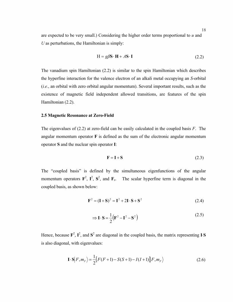
18are expected to be very small.) Considering the higher order terms proportional to u and
U as perturbations, the Hamiltonian is simply:
ISHS ⋅+⋅=Η Agβ (2.2)
The vanadium spin Hamiltonian (2.2) is similar to the spin Hamiltonian which describes
the hyperfine interaction for the valence electron of an alkali metal occupying an S-orbital
(i.e., an orbital with zero orbital angular momentum). Several important results, such as the
existence of magnetic field independent allowed transitions, are features of the spin
Hamiltonian (2.2).
2.5 Magnetic Resonance at Zero-Field
The eigenvalues of (2.2) at zero-field can be easily calculated in the coupled basis F. The
angular momentum operator F is defined as the sum of the electronic angular momentum
operator S and the nuclear spin operator I:
SIF += (2.3)
The “coupled basis” is defined by the simultaneous eigenfunctions of the angular
momentum operators F2, I2, S2, and Fz. The scalar hyperfine term is diagonal in the
coupled basis, as shown below:
2222 2)( SSIISIF +⋅+=+= (2.4)
( )222
21 SIFSI −−=⋅⇒
(2.5)
Hence, because F2, I2, and S2 are diagonal in the coupled basis, the matrix representing I⋅S
is also diagonal, with eigenvalues:
[ ] FF mFIISSFFmF ,)1()1()1(21, +−+−+=⋅SI (2.6)
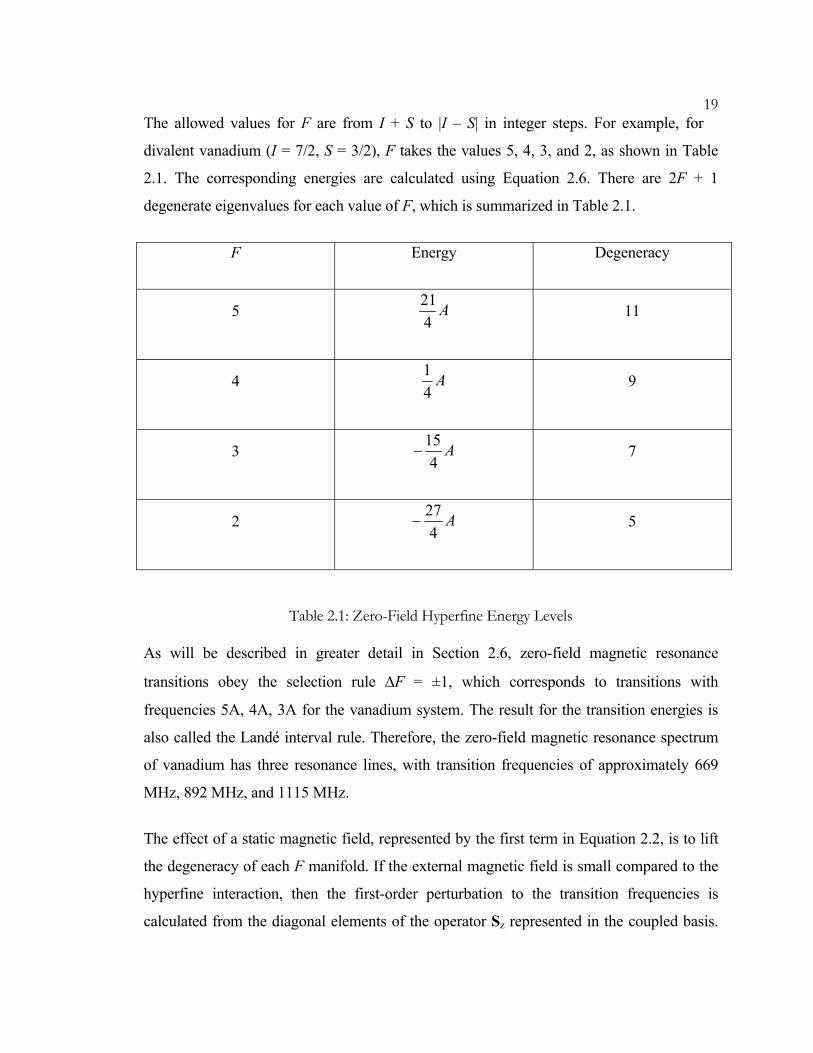
19The allowed values for F are from I + S to |I – S| in integer steps. For example, for
divalent vanadium (I = 7/2, S = 3/2), F takes the values 5, 4, 3, and 2, as shown in Table
2.1. The corresponding energies are calculated using Equation 2.6. There are 2F + 1
degenerate eigenvalues for each value of F, which is summarized in Table 2.1.
F Energy Degeneracy
5 A421 11
4 A41 9
3 A4
15− 7
2 A4
27− 5
Table 2.1: Zero-Field Hyperfine Energy Levels
As will be described in greater detail in Section 2.6, zero-field magnetic resonance
transitions obey the selection rule ∆F = ±1, which corresponds to transitions with
frequencies 5A, 4A, 3A for the vanadium system. The result for the transition energies is
also called the Landé interval rule. Therefore, the zero-field magnetic resonance spectrum
of vanadium has three resonance lines, with transition frequencies of approximately 669
MHz, 892 MHz, and 1115 MHz.
The effect of a static magnetic field, represented by the first term in Equation 2.2, is to lift
the degeneracy of each F manifold. If the external magnetic field is small compared to the
hyperfine interaction, then the first-order perturbation to the transition frequencies is
calculated from the diagonal elements of the operator Sz represented in the coupled basis.

20Generally, the representation of an angular momentum operator S in the coupled basis
will be a product of one factor which depends only on the quantum number F, and a second
factor involving both F and mF. The complete calculation of the matrix representing an
angular momentum operator in the coupled basis is detailed in Condon & Shortley [13].
For example, the diagonal elements of Sz are:
FB
FFZB
SF mgmFgmF hhh
µµ=,, S (2.7)
where gF is called the Landé g-factor, equal to:
⎥⎦
⎤⎢⎣
⎡+
+−+++=
)1(2)1()1()1(
FFIISSFFgg SF
(2.8)
For S = 3/2 and I = 7/2, the Landé g-factor is
⎥⎦
⎤⎢⎣
⎡+−+
=)1(2
)12)1(FF
FFgg SF
(2.9)
The Landé factors for the F-states of V++ are shown in Table 2.2 below.

21
F gF-factor F(F+1) F(F+1)gF2
5 Sg103
30 2
1027
Sg
4 Sg102
20 2
108
Sg
3 0 12 0
2 Sg21
−
6 2
1015
Sg
Table 2.2: Landé factors to calculate Zeeman shift for the F-states of V++
The Zeeman shift of a resonance line is determined by the difference of the Landé factors
and quantum numbers mF of the initial and final states. There are 2F + 1 Zeeman levels in
each F manifold corresponding to the eigenvalues mF = {F, F − 1, F − 2, …, −|F − 1|, −F}.
The Zeeman shift for each set of F sublevels of V++/MgO is plotted in Figure 2.1:

22
0 10 20 30 40 50 60 70 80 90 100-2000
-1500
-1000
-500
0
500
1000
1500
2000
Magnetic Field (Gauss)
Hyp
erfin
e E
nerg
y (M
Hz)
Figure 2.1: Numerically Calculated Zeeman Shift for V++/MgO
In the figure, the exact eigenvalues are used from a numerical solution to Equation 2.2 at
each value of the applied magnetic field H. The second-order Zeeman shift is evident at
magnetic fields above approximately 50 Gauss. For Zeeman fields from 0 to 20 Gauss, the
first-order theory is a close approximation to the exact solution.
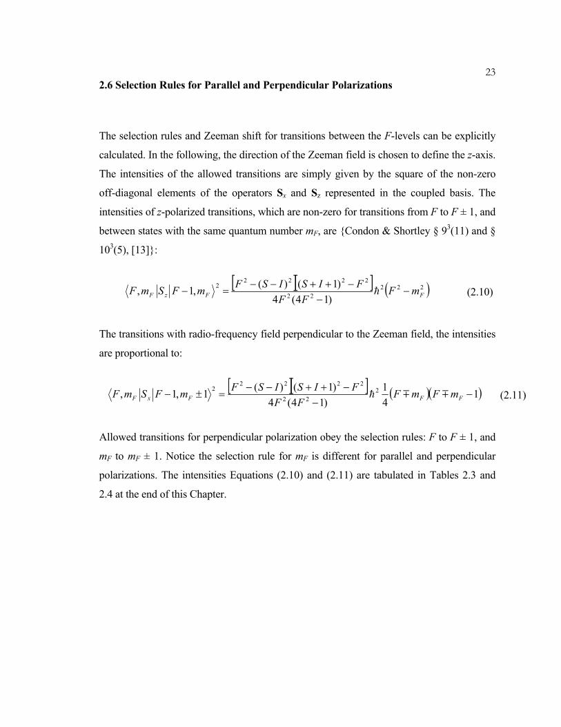
232.6 Selection Rules for Parallel and Perpendicular Polarizations
The selection rules and Zeeman shift for transitions between the F-levels can be explicitly
calculated. In the following, the direction of the Zeeman field is chosen to define the z-axis.
The intensities of the allowed transitions are simply given by the square of the non-zero
off-diagonal elements of the operators Sx and Sz represented in the coupled basis. The
intensities of z-polarized transitions, which are non-zero for transitions from F to F ± 1, and
between states with the same quantum number mF, are {Condon & Shortley § 93(11) and §
103(5), [13]}:
[ ][ ] ( )22222
22222
)14(4)1()(,1, FFzF mF
FFFISISFmFSmF −
−−++−−
=− h (2.10)
The transitions with radio-frequency field perpendicular to the Zeeman field, the intensities
are proportional to:
[ ][ ] ( )( 141
)14(4)1()(1,1, 2
22
22222 −
−−++−−
=±− FFFxF mFmFFF
FISISFmFSmF mmh ) (2.11)
Allowed transitions for perpendicular polarization obey the selection rules: F to F ± 1, and
mF to mF ± 1. Notice the selection rule for mF is different for parallel and perpendicular
polarizations. The intensities Equations (2.10) and (2.11) are tabulated in Tables 2.3 and
2.4 at the end of this Chapter.
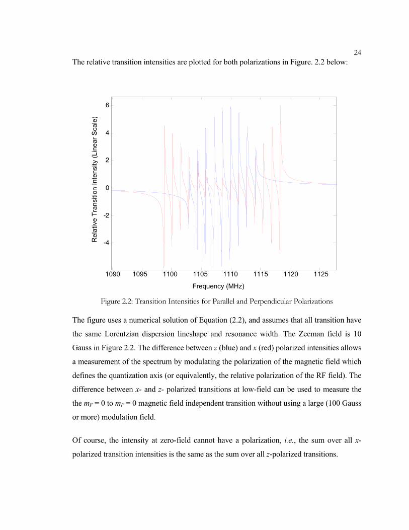
24The relative transition intensities are plotted for both polarizations in Figure. 2.2 below:
Rel
ativ
e Tr
ansi
tion
Inte
nsity
(Lin
ear S
cale
)
1090 11251095 1100 1105 1110 1115 1120
Frequency (MHz)
-4
-2
0
2
4
6
Figure 2.2: Transition Intensities for Parallel and Perpendicular Polarizations
The figure uses a numerical solution of Equation (2.2), and assumes that all transition have
the same Lorentzian dispersion lineshape and resonance width. The Zeeman field is 10
Gauss in Figure 2.2. The difference between z (blue) and x (red) polarized intensities allows
a measurement of the spectrum by modulating the polarization of the magnetic field which
defines the quantization axis (or equivalently, the relative polarization of the RF field). The
difference between x- and z- polarized transitions at low-field can be used to measure the
the mF = 0 to mF = 0 magnetic field independent transition without using a large (100 Gauss
or more) modulation field.
Of course, the intensity at zero-field cannot have a polarization, i.e., the sum over all x-
polarized transition intensities is the same as the sum over all z-polarized transitions.

252.7 Magnetic Susceptibility
This section calculates the resonant magnetic susceptibility due to magnetic resonance
transitions of the type described in Section (4).
The transition rate between the zero-field hyperfine levels is given by (c.f. Yariv, 1967 ref.
[2]):
)(1 2'2 νgHW kmkmh
=→
(2.12)
where g(ν) is a normalized lineshape function:
∫∞
∞−
= 1)( kk dg νν
(2.13)
The transition rate for the z-polarized F = 5 to F = 4 magnetic field independent transition
is:
)(0583.0)(990005775 2
1
2
, νωνµ
ggHg
W RFzBS
km =⎟⎠⎞
⎜⎝⎛=→
h (2.14)
where Hz,RF is the magnitude of the RF magnetic field. The magnetic susceptibility is
(Yariv 1967, (8.2-2) [2]):
[ 0,40,5
2
)(20583.0)('' ==== −⎟⎠⎞
⎜⎝⎛⋅= MFMF
BS NNgg
νµ
υχh
h ]
(2.15)
The thermal population difference is
NkT
NN MFMF0
0,40,52
321 πνh
≅− ====
(2.16)

26where N is the density of paramagnetic ions and ν0 is the resonant frequency. Suppose
the g(ν) is Lorentzian with “half-power” width of ∆ν:
])2/()[(2)( 22
00 vvv
vvvg∆+−
∆=−
π (2.17)
vg
∆=
π2)0(
(2.18)
Therefore, the magnetic susceptibility due to the z-polarized 0-0 transition is:
NkTvvv
vg BS 022
0
2
02
321
])2/()[(220583.0)(''
πνπ
µυχ
h
hh
∆+−∆
⎟⎠⎞
⎜⎝⎛⋅=
(2.19)
( )N
vvvv
kTg BS
])2/()[(1610583.0)('' 22
0
02
0 ∆+−∆
⋅=νµ
υχ
(2.20)
As an example, we calculate the resonant magnetic susceptibility for a magnesium oxide
crystal doped with 100 ppm vanadium relative to the anion lattice. The concentration of
spin is:
ccmolppmmolg
ccgN /1035.5)10022.6(1003.2416
58.3 18123 ×=×××+
= −
(2.21)
The physical constants are (in CGS units):
( ) 227116
21212
1029.8300)1038.1(
)10264.92( −−−−
−−
×=⋅×
×⋅= ergG
KergKergG
kTg BSµ
(2.22)
ccvvv
vergG /1035.5
])2/()[(1029.8
1610583.0)('' 18
220
02270 ×
∆+−∆
×⋅= −− νυχ
(2.23)
27
The numerical expression for the magnetic susceptibility is:
])2/()[(1062.1)('' 22
0
012100 vvv
vccergG
∆+−∆
×= −−− νυχ
(2.24)
Converting to MKS units, the equivalent magnetic susceptibility is:
])2/()[(1004.2)(''4 22
0
090 vvv
v∆+−
∆×= − ν
υπχ
(2.25)
which for a 5 MHz wide resonance at 1110 MHz is equal to 1.81 × 10⁻⁶.
The total zero-field intensity for 5 MHz and 100 ppm is 6.6*1.81 = 1.2 × 10⁻⁵.
2.8 Circuit Model for Electrical Resonator Containing Paramagnetic Sample
.
A model for an electrical resonator containing a paramagnetic sample is now easily
developed using the magnetic susceptibility. The effective inductance of the loop-gap
resonator or other resonator containing the paramagnetic sample is modified by the change
in magnetic susceptibility:
)41(0 πηχ+= LL (2.26)
The fill factor is equal to:
∫
∫=
cavity
sample
dvH
dvH
21
21
η
(2.27)

28In the present experiment, the fill factor is approximately 1/3.
(ii) Calculate the frequency modulation of the resonator due to paramagnetic sample
The resonant frequency is:
( )LC12 2
0 =πν
(2.28)
and for a small change in inductance, the frequency perturbation is:
πηχνν
421
21
0
0 −=∂
−=∂
LL
(2.29)
(iii) Calculate the resonator frequency modulation introduced phase modulation to the
transmitted carrier. The electrical resonator dispersion at resonance is:
00
2νν
θ LQ=
∂∂
(2.30)
The phase-modulation introduced by the paramagnetic resonance is therefore
χπηθ LQ4−=∂ (2.31)
The single-sideband power due to phase modulation is:
RMSLQP χπη4log20= (2.32)
For example, if the fill factor is 1/3 and the loaded-Q is 250, the sideband power due to 5
MHz wide transition with intensity of Z, 0-0, is -76 dBc.
(iv) Calculate the sensitivity assuming thermal noise limit
29The thermal noise power kT is equal to -174 dBm. If the receiver has a 3dB noise figure,
the noise floor is -171 dBm. The theoretical sensitivity is therefore 95 dB from a 0dBm
carrier.
2.9 Numerical Calculation of Eigenvalues and Transition Intensities
Another very useful technique is to numerically solve for the eigenvalues and energies of
the spin Hamiltonian, then plot the spectrum by generating a matrix with the frequencies
and intensities of the magnetic dipole transitions. An example shown below is the spectrum
of Mn++ ion at zero field, which is more complex that the V++ spectrum because of the non-
zero crystal field terms in the spin Hamiltonian for S = 5/2 in cubic symmetry. The
spectrum is calculated using published values for the hyperfine interaction and crystal field
term determined from high-field measurements [13,14].
The zero-field magnetic resonance measurements presented in this thesis measure the
dispersion introduced by the paramagnetic resonance of the sample (i.e., the real
component of the magnetic susceptibility), rather than measuring absorption (i.e., the
imaginary component of the magnetic susceptibility.) When comparing experimental
results to calculation, the spectrum assumes Lorentzian dispersion lineshapes for all
transitions, modeled using the function:
])2/()[(2)()( 22
0
00 vvv
vvvvvg∆+−
−∆=−
π (2.33)
The measured spectrum is the difference between the dispersive component of the
magnetic susceptibility at zero magnetic field and the dispersive component of the
magnetic susceptibility at the peak Zeeman modulation field. These aspects of the magnetic
resonance measurement are detailed in Chapter 4.

30
Rel
ativ
e M
agne
tic S
usce
ptib
ility
(Lin
ear S
cale
)
500 600 700 800 900 1000 1100 1200 1300-4
-3
-2
-1
0
1
2
3
4
Frequency (MHz)
Figure 2.3: Calculated Spectrum for Mn++ in Magnesium Oxide
A typical calculation is shown in Figure 2.3 above, calculated using the published
parameters for the spin Hamiltonian of Mn++/MgO. The numerical model does not account
for the variations in dipolar resonance widths, discussed in Chapter 3. The spectrum shows
that Mn++ ions in a magnesium oxide sample have zero-field paramagnetic resonance
signals in the range of 500 to 1300 MHz.
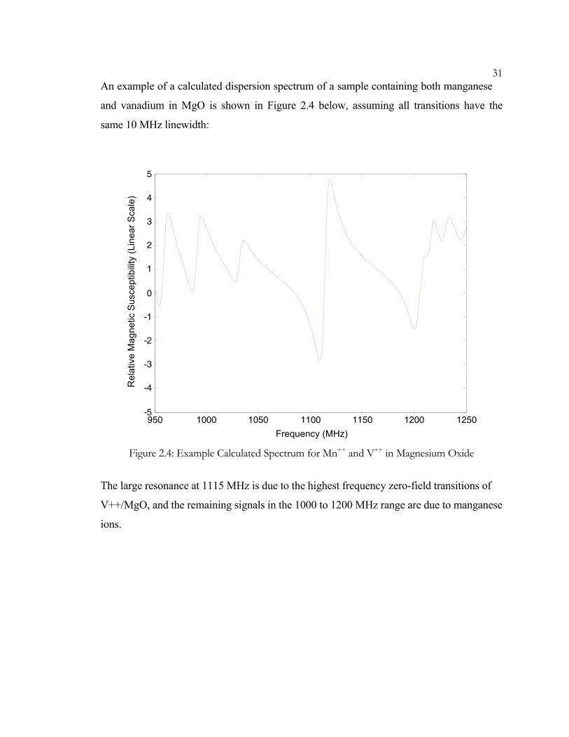
31An example of a calculated dispersion spectrum of a sample containing both manganese
and vanadium in MgO is shown in Figure 2.4 below, assuming all transitions have the
same 10 MHz linewidth:
950 1000 1050 1100 1150 1200 1250-5
-4
-3
-2
-1
0
1
2
3
4
5
Rel
ativ
e M
agne
tic S
usce
ptib
ility
(Lin
ear S
cale
)
Frequency (MHz)
Figure 2.4: Example Calculated Spectrum for Mn++ and V++ in Magnesium Oxide
The large resonance at 1115 MHz is due to the highest frequency zero-field transitions of
V++/MgO, and the remaining signals in the 1000 to 1200 MHz range are due to manganese
ions.

322.10 Comparison to Measurement
A measured zero-field paramagnetic spectrum of a sample of magnesium oxide containing
both vanadium and manganese is shown below in Figure 2.5. The modulation field was
approximately 12 Gauss. Details of the zero-field spectrometer design are described in
Chapter 4. The red curve is the measured spectrum and the blue curve is a calculation. We
can see that the basic features of the calculated and measured spectrum are the same. The
zero-field measurement allows for a more precise determination of the hyperfine coupling
which is seen to be approximately 1% lower than the published value determined from
high-field measurements [14].
Frequency (MHz)
1000 1020 1040 1060 1080 1100 1120 1140 1160 1180 1200
-10
-8
-6
-4
-2
0
2
4
Volts
at S
pect
rom
eter
Out
put
Cal
cula
ted
Rel
ativ
e M
agne
tic S
usce
ptib
ility
(Lin
ear S
cale
)
Figure 2.5: Measured Spectrum for Mn++ and V++ in Magnesium Oxide
33The measured curve is the output in volts from the zero-field magnetic resonance
spectrometer described in Chapter 4. The blue curve was calculated similar to Figure 2.4,
using published parameters for V++ and Mn++ ions in magnesium oxide known from high-
field measurements. The relative intensities of the vanadium and manganese spectrum, as
well as the resonance widths, were adjusted to approximately match the measured
spectrum. Therefore, the measurement in Figure 2.5 validates the model of zero-field
magnetic resonance presented in this chapter. Chapter 3 will discuss the linewidths at zero-
field in greater detail.
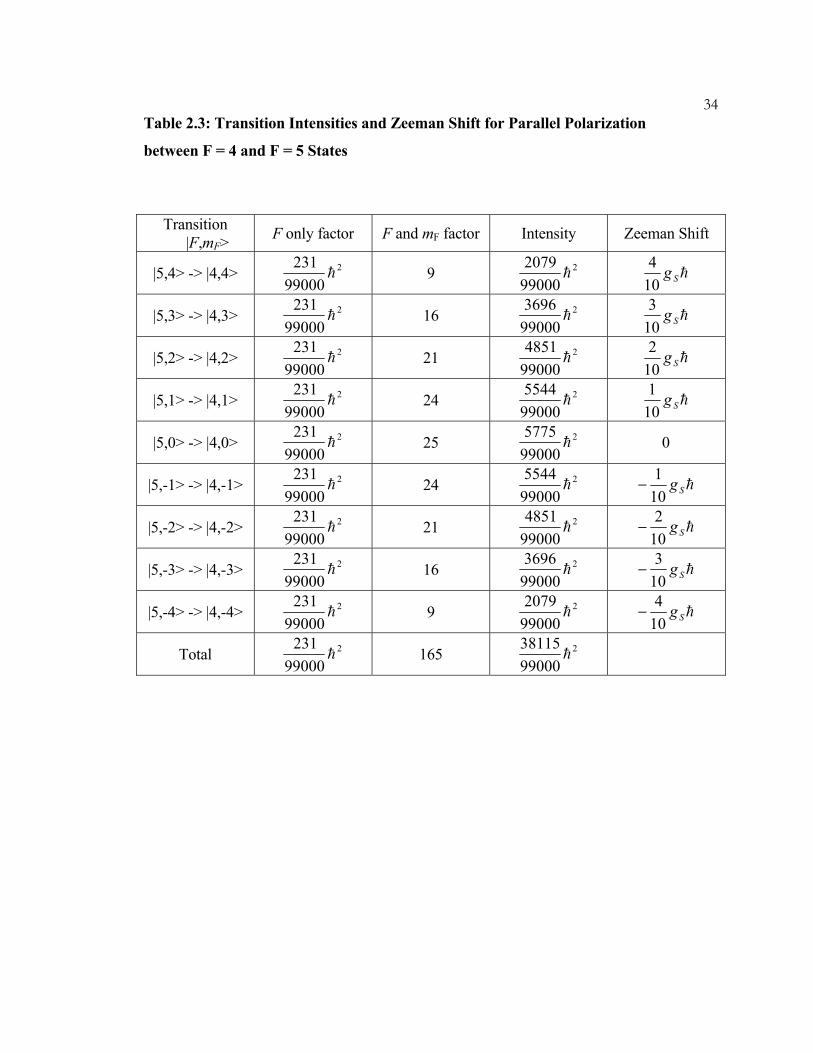
34Table 2.3: Transition Intensities and Zeeman Shift for Parallel Polarization
between F = 4 and F = 5 States
Transition |F,mF> F only factor F and mF factor Intensity Zeeman Shift
|5,4> -> |4,4> 2
99000231
h
9 2
990002079
h
hSg104
|5,3> -> |4,3> 2
99000231
h
16 2
990003696
h
hSg103
|5,2> -> |4,2> 2
99000231
h
21 2
990004851
h
hSg102
|5,1> -> |4,1> 2
99000231
h
24 2
990005544
h
hSg101
|5,0> -> |4,0> 2
99000231
h
25 2
990005775
h
0
|5,-1> -> |4,-1> 2
99000231
h
24 2
990005544
h
hSg101
−
|5,-2> -> |4,-2> 2
99000231
h
21 2
990004851
h
hSg102
−
|5,-3> -> |4,-3> 2
99000231
h
16 2
990003696
h
hSg103
−
|5,-4> -> |4,-4> 2
99000231
h
9 2
990002079
h
hSg104
−
Total 2
99000231
h
165 2
9900038115
h
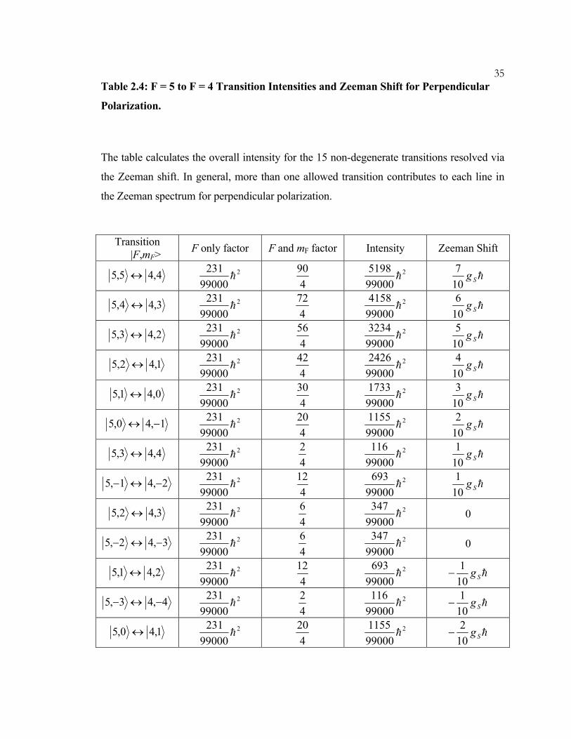
35Table 2.4: F = 5 to F = 4 Transition Intensities and Zeeman Shift for Perpendicular
Polarization.
The table calculates the overall intensity for the 15 non-degenerate transitions resolved via
the Zeeman shift. In general, more than one allowed transition contributes to each line in
the Zeeman spectrum for perpendicular polarization.
Transition
|F,mF> F only factor F and mF factor Intensity Zeeman Shift
4,45,5 ↔ 2
99000231
h 4
90 2
990005198
h hSg107
3,44,5 ↔ 2
99000231
h 4
72 2
990004158
h hSg106
2,43,5 ↔ 2
99000231
h 4
56 2
990003234
h hSg105
1,42,5 ↔ 2
99000231
h 4
42 2
990002426
h hSg104
0,41,5 ↔ 2
99000231
h 4
30 2
990001733
h hSg103
1,40,5 −↔ 2
99000231
h 4
20 2
990001155
h hSg102
4,43,5 ↔ 2
99000231
h 4
2 2
99000116
h hSg101
2,41,5 −↔− 2
99000231
h 4
12 2
99000693
h hSg101
3,42,5 ↔ 2
99000231
h 4
6 2
99000347
h 0
3,42,5 −↔− 2
99000231
h 4
6 2
99000347
h 0
2,41,5 ↔ 2
99000231
h 4
12 2
99000693
h hSg101
−
4,43,5 −↔− 2
99000231
h 4
2 2
99000116
h hSg101
−
1,40,5 ↔ 2
99000231
h 4
20 2
990001155
h hSg102
−
36
0,41,5 ↔− 2
99000231
h 4
30 2
990001733
h hSg103
−
1,42,5 −↔− 2
99000231
h 4
42 2
990002426
h hSg104
−
2,43,5 −↔− 2
99000231
h 4
56 2
990003234
h hSg105
−
3,44,5 −↔− 2
99000231
h 4
72 2
990004158
h hSg106
−
4,45,5 −↔− 2
99000231
h 4
90 2
990005198
h hSg107
−
Total 2
99000231
h
165 2
9900038115
h
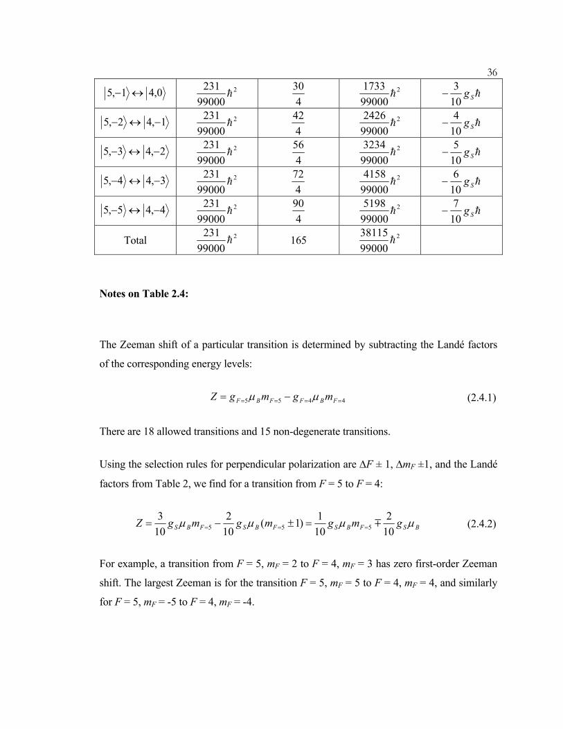
Notes on Table 2.4:
The Zeeman shift of a particular transition is determined by subtracting the Landé factors
of the corresponding energy levels:
4455 ==== −= FBFFBF mgmgZ µµ (2.4.1)
There are 18 allowed transitions and 15 non-degenerate transitions.
Using the selection rules for perpendicular polarization are ∆F ± 1, ∆mF ±1, and the Landé
factors from Table 2, we find for a transition from F = 5 to F = 4:
BSFBSFBSFBS gmgmgmgZ µµµµ102
101)1(
102
103
555 m=== =±−= (2.4.2)
For example, a transition from F = 5, mF = 2 to F = 4, mF = 3 has zero first-order Zeeman
shift. The largest Zeeman is for the transition F = 5, mF = 5 to F = 4, mF = 4, and similarly
for F = 5, mF = -5 to F = 4, mF = -4.

37
BIBLIOGRAPHY, CHAPTER 2
[1] J. R. Pilbrow, Transition Ion Electron Paramagnetic Resonance, Clarendon Press Oxford, 1990.
[2] J. E. Wertz and J. R. Bolton, Electron Spin Resonance: Elementary Theory and
Practical Applications, Chapman and Hall Ltd., 1986. [3] Charles P. Poole, Jr. and Horacia A. Farach, Handbook of Electron Spin Resonance,
Volume 1 and 2, Springer-Verlag New York, Inc., 1999. [4] Charles P. Poole, Jr., Electron Spin Resonance: A Comprehensive Treatise on
Experimental Techniques, Wiley, 1983. [5] A. Abragam and B. Bleaney, Electron Paramagnetic Resonance of Transition Ions,
Clarendon Press, Oxford, 1970. [6] Christopher D. Delfs and Richard Bramley, “Zero-field Electron Magnetic Resonance
Spectra of Copper Carboxylates,” J. Chem. Phys., vol. 107, pp. 8840, 1997. [7] Christopher D. Delfs and Richard Bramely, “The Zero-field ESR Spectrum of a Copper
Dimmer,” Chemical Physics Letters, vol. 264, pp. 333, 1997. [8] Richard Bramley and Steven J. Strach, “Zero-Field EPR of the Vanadyl Ion in
Ammonium Sulfate,” J. of Magnetic Resonance, vol. 61, pp. 245, 1985. [9] Richard Bramley and Steven J. Strach, “Electron Paramagnetic Resonance
Spectroscopy at Zero Magnetic Field,” Chem. Rev., vol. 83, pp. 49-82, 1983. [10] Cole, T. Kushida, T., and Heller, H. C., “Zero-Field Electron Magnetic Resonance in
Some Inorganic and Organic Radicals,” J. Chem. Phys., vol. 38, pp. 2915, 1963. [11] P. R. Solomon, “Relaxation of Mn2+ and Fe3+ Ions in Magnesium Oxide,” Phys. Rev.,
vol. 152, no. 1, December 1966. [12] Walter M. Walsh, Jr., Jean Jeener, and N. Bloembergen, “Temperature-Dependent
Crystal Field and Hyperfine Interactions,” Phys. Rev., vol. 139, pp. A 1338, 1965. [13] E. U. Condon & G. H. Shortley, The Theory of Atomic Spectra, Cambridge University
Press, 1963.
38[14] W. Low, “Paramagnetic Resonance Spectra of Some Ions in the 3d and 4f Shells in
Cubic Crystalline Fields,” Phy. Rev., vol. 101, pp. 1827, 1956. [15] J.E. Wertz, J. W. Orton, and P. Auzins, “Spin Resonance of Point Defects in
Magnesium Oxide,” J. Appl. Phys., vol. 33, no. 1, pp. 322-328, 1962. [16] R. S. De Biasi, “Influence of the S3 Term on the EPR Spectrum of Cr3+ in Cubic
Symmetry Sites in MgO,” Journal of Magnetic Resonance, vol. 44, pp. 479-482, 1981. [17] A. J. Freeman, R. B. Frankel eds., Hyperfine Interactions, Academic Press New York,
1967, c.f. Ch 1 by B. Bleaney. [18] Richard Bramley, personal communication [19] A. Yariv, Quantum Electronics, Wiley, 1st ed., 1967.