2.2. instantaneous velocity toc assuming that your …dpstory/tutorial/c1/c1l_t1.pdfsection 2:...

Section 2: Motivating the Concept ~wtoc2.2. Instantaneous Velocity

Assuming that your are not familiar with the technical aspects ofthis section, when you think about it, your knowledge of velocityis limited. In terms of your own mathematical background, there isonly one type of velocity you can deal with: Constant Velocity. Tomake matters worse, there is really only one formula for dealing withvelocity: the famous formula,

distance = velocity× time. (4)

But the good news is that simple algebra is sufficient to solve manyproblems involving constant velocity. The bad news is that, based onlife’s experiences, velocity is hardly ever constant!

One way around this problem is through the notion of average veloc-ity. Even though the average velocity concept is very useful in manydifferent situations, it is inadequate for a deeper study of the dynamicsof motion of a particle. For this reason, we need a better understand-ing of velocity. This requires us to move to a higher mathematicalplane: The Calculus level.

Section 2: Motivating the Concept

It was the limit concept that enabled mathematicians to move fromthe algebraic level to the Calculus level.

First, we begin with a . . .

Review of Average Velocity. Suppose, for simplicity, a particle ismoving in a straight line, and this straight line is the traditional x-axis. At time t = t0 the particle is at position x = a, at a later time,t = t1, the particle is observed to be at position x = b. Thus, theparticle has moved from point a to point b during the time interval[ t0, t1 ]. By definition, the average velocity of the particle during thetime interval [ t0, t1 ] is

vavg :=b− at1 − t0 . (5)

Or, in mere words, the average velocity is the distance traveled (b−a)divided by the time (t1 − t0) needed to travel that distance.

Exercise 2.2. It is possible for vavg to be positive, negative, or zero.Explain each case physically.


What is average velocity?

vavg is the constant velocity the particle would have to travelat in order to go from position x = a to x = b during thetime interval [ t0, t1 ], if the particle was moving at constantvelocity.

(But, of course, if this was a teenage particle its velocity would defi-nitely not be constant!)

An algebraic proof of this assertion follows. Here, we assume that theparticle is moving at a constant velocity, vconst, and that we have twodata points: at time t = t0, the particle is at x = a; and at time t = t1,the particle is at x = b.

Recall equation (4), and its variant,

distance = (velocity)× (time),or,


velocity =distance

time, (6)

which is valid only in the case of constant velocity. Thus,

distance = b− avelocity = vconst

time = t1 − t0.Substitute into (6) to get

vconst =b− at1 − t0

= vavg. (7)

The last equality in line (7) comes from the definition of averagevelocity in equation (5).

Exercise 2.3. (Skill Level 0) An automobile was observed to travel30 miles in one-half hour. What is the average velocity of the auto-mobile? What is the average velocity as measured in ft/sec?


Instantaneous Velocity. Now let’s begin our discussion of the newconcept of instantaneous velocity as an application to the limit con-cept. Suppose we have a particle moving in a straight line (the x-axis,say). Define a function as follows: at any time t,

f(t) := position on x-axis at time t.

Problem: Fix a time point t = t0, define/calculate the notion of theinstantaneous velocity of the particle at time t = t0; i.e., we want toknow the velocity of the particle at the instant in time t = t0. (I say‘define/calculate,’ because this is a ‘new’ notion (define), yet, I wanta calculating formula (calculate).)

This notion of instantaneous velocity, intuitively, is characterized bythe position (as determined by the function f) of the particle aroundthe time in question, t = t0. Such a phrase suggests the limit concept.(see above.)


Let us begin by interpreting various quantities: Let h > 0 be a positive(time) value,

t0 = the time of interestt0 + h = the time h time units after t0f(t0) = position at time t0

f(t0 + h) = position at time t0 + h.Also,

f(t0 + h)− f(t0) = distance traveled during thetime interval [ t0, t0 + h ]

and finally,f(t0 + h)− f(t0)

h= average velocity of the particle

during the interval [ t0, t0 + h ](8)

The last equation (8) follows from the definition of average velocity,and the observation that the length of the time interval [ t0, t0 + h ] is(t0 + h)− t0 = h.


To continue, let us take a particular function so we can make somenumerical calculations to illustrate the idea. Take,

f(t) = t2, and t0 = 2.

Note that in equation (8), t0 is fixed (the time point of interest),the only variable quantity is the time increment h. We are interestedin studying the velocity of the particle in smaller and smaller timeintervals around the point of interest t = t0. The point of the abovediscussion is that the expression in (8) depends on the value of h;hence defines a function of h. Define, therefore,

vavg(h) :=f(t0 + h)− f(t0)

h(9)


Now, for the purpose of illustration, we are taking f(t) = t2, andt0 = 2. Then, in this case, (9) becomes

vavg(h) =f(t0 + h)− f(t0)

h

=f(2 + h)− f(2)

h

=(2 + h)2 − 4

h

=(4 + 4h+ h2)− 4

h

=4h+ h2

h= 4 + h.

Thus,vavg(h) = 4 + h (10)

Equation (10) is equation (8) specialized to f(t) = t2, and t0 = 2.


Now you can clearly see the meaning of my comment above: In equa-tion (10) we have the average velocity in an interval around the timepoint t0 = 2 of interest is written explicitly as a function of h, thelength of that interval.

What happens as the length of the time interval gets smaller; that is,what happens to average velocity as h gets closer and closer to 0? Itshould be obvious from (10): If h ≈ 0, then vavg ≈ 4. I’ll construct atable anyway:

vavg = 4 + hh 1.0 0.5 0.1 0.05 0.01 0.005 0.001

vavg 5.0 4.5 4.1 4.05 4.01 4.005 4.001

Let’s interpret the entries of the table. I’ll assume the scales of mea-surements are feet and seconds. For example, vavg(.01) = 4.01 meansthat from time t = 2 to t = 2.01, the particle averaged 4.01 ft/sec;vavg(.001) = 4.001 means that from time t = 2 to t = 2.001, the parti-cle averaged 4.001 ft/sec. Finally, not included in the table is that theparticle averaged 4.000001 ft/sec over the time interval [ 2, 2.000001 ].


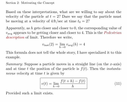
Based on these interpretations, what are we willing to say about thevelocity of the particle at t = 2? Dare we say that the particle mustbe moving at a velocity of 4 ft/sec at time t0 = 2?

Apparently, as h gets closer and closer to 0, the corresponding value ofvavg appears to be getting closer and closer to 4. This is the Pedestriandescription of limit. Therefore we write,

vinst(2) = limh→0

vavg(h) = 4

This formula does not tell the whole story, I have specialized it to thisexample.

Summary : Suppose a particle moves in a straight line (on the x-axis)and at time t the position of the particle is f(t). Then the instanta-neous velocity at time t is given by

v(t) = limh→0

f(t+ h)− f(t)h

(11)

Provided such a limit exists.


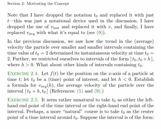
Note that I have dropped the notation t0 and replaced it with justt—this was just a notational device used in the discussion. I havedropped the use of vinst and replaced it with v, and finally, I havereplaced vavg with what it’s equal to (see (9)).

In the previous discussion, we saw how the trend in the (average)velocity the particle over smaller and smaller intervals containing thetime value of t0 = 2 determined its instantaneous velocity at time t0 =2. Further, we restricted ourselves to intervals of the form [ t0, t0 +h ],where h > 0. What about other kinds of intervals containing t0.

Exercise 2.4. Let f(t) be the position on the x-axis of a particle attime t; let t0 be a (time) point of interest, and let h < 0. Establisha formula for vavg(h), the average velocity of the particle over theinterval [ t0 + h, t0 ] (References: (5) and (9).)

Exercise 2.5. It seem rather unnatural to take t0 as either the left-hand end point of the time interval or the right-hand end point of theinterval. Perhaps, a more “natural” course is to take t0 as the centerpoint of a time interval around t0. Suppose the interval is of the form:


[ t0 − h, t0 + h ], where h > 0. Construct a formula for vavg(h), theaverage velocity of the particle over this interval.

2.3. Tangent to a Curve

We begin by stating the basic problem of this section, which, at thisintroductory level to calculus, is usually thought of as the origin ofdifferential calculus. In most calculus books, this problem is alwaysadvertised as the . . .

Fundamental Problem of Differential Calculus. Given a curve and apoint on that curve, define/calculate the equation of the line tangentto the given curve at the given point.

History. Mathematically, the notion of tangent line has already beendefined in your past history. If you have taken a course (in highschool), in Plane Geometry, you would have come across the followingtheorem due to Euclid:

Given a circle in the plane, and a line in the plane, then exactlyone of the following is true: (1) the line does not touch the circle;


(2) the line touches the circle at one point; (3) the line touchesthe circle at two points.

Remarks: In case (2), we say the line is tangent to the circle. The linedescribed in case (3) is referred to as a secant line.

This is the sum total of your knowledge of tangent lines. Yet, it issufficient to give you an intuitive notion of what is meant by a tangentline to an arbitrary curve.

Solution to the Problem. We need a curve. This problem willeventually be solved in greater generality, but until then we take asimple, yet important, case. Take the curve to be of the form:

The Curve: y = f(x) (10)Now we need a point on the curve.

The Point: P ( a, f(a) ) (11)

We want to construct the equation of a line having the property thatthe line passes through the given point P ( a, f(a) ), and having a cer-tain intuitive property: tangency. We need to define our line so thatit has this vaporous property.


In order to construct the equation of a line we need one of two sets ofinformation about that line: (1) We need two points on the line; (2)we need one point on the line and the slope of the line. Note that wehave neither of these two. This is the basic problem — we don’t haveenough information. We have one point, but we don’t have a secondpoint, nor do we have the slope of the line.

The tack we take to solve the problem is to define/calculate the slopeof the imagined tangent line. If we have the slope, then we can writedown the equation of the tangent line: we have a point and the slope.

To construct a line we need a second point. Let h > 0 be a smallnumber. Consider x = a and x = a + h. These two values of x are hunits apart. Now look at the corresponding points on the curve:

P ( a, f(a) ) Q( a+ h, f(a+ h) ).

If h is small, the point Q is close to the point P . Draw a line throughthese two points. This line is called a secant line. The slope of this


line can be computed as

msec(h) =f(a+ h)− f(a)

(a+ h)− aThus,

msec(h) =f(a+ h)− f(a)

h. (12)

Notice that I have represented the slope of the line through the pointsP andQ as a function of h; this seems reasonable sinceQ is determinedby the value of h and so the slope of this line depends on the choiceof Q, which in turn depends on h.

Figure 1The line through P and Q:the secant line approximatesy = f(x) near P .

Figure 2An approximating secant lineshown with the hypotheticaltangent line.

Figure 1 depicts the secant line through the points P and Q; it’s slopeis given in equation (12). While in Figure 2 the tangent line has beenincluded. Now imagine, if you can, how the picture changes as h gets


closer and closer to 0: the point Q moves along the curve gettingcloser and closer to the point P ; the secant line rotates around thepivot point P and becomes more and more tangent-like. Now if thesecant line is looking more and more like a tangent line, then the slopeof the secant line must be getting closer and closer to the slope of the(imagined) tangent line.

Let’s summarize the major points of the above discussion: As h getscloser and closer to 0, the slope of the secant line, msec(h), we imag-ine, will get closer and closer to mtan, we imagine. But this is thePedestrian description of limit!

mtan = limh→0

msec(h)

= limh→0

f(a+ h)− f(a)h

/ by (12)

or,

mtan = limh→0

f(a+ h)− f(a)h


Let’s have some numerical calculations for you unbelievers in thepeanut gallery.

Example 2.2. Consider the function f(x) =√x, and take a = 4. Set

up a table of secant slopes and try to determine the slope of the linetangent to the graph of f at a = 4.

The table given in the solution to Example 2.2, only positive valuesof h were used. What about negative values of h? Perhaps the use ofnegative values of h lead us to an entirely different conclusion thanbefore.

Exercise 2.6. Take the table given in the solution to Example 2.2,negate each of the values of h, and re-calculate the corresponding valesof msec.

That’s enough for an introduction to the concept of limit and howit is applied to solve the fundamental problem of differential calculus.You’ll get plenty more in your regular calculus course as well as inthese tutorials.


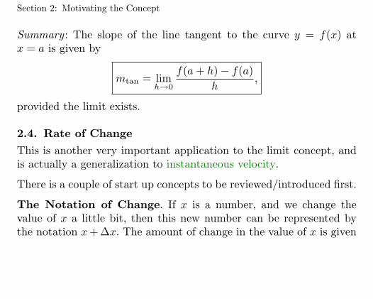
Summary : The slope of the line tangent to the curve y = f(x) atx = a is given by

mtan = limh→0

f(a+ h)− f(a)h

,

provided the limit exists.

2.4. Rate of Change

This is another very important application to the limit concept, andis actually a generalization to instantaneous velocity.

There is a couple of start up concepts to be reviewed/introduced first.

The Notation of Change. If x is a number, and we change thevalue of x a little bit, then this new number can be represented bythe notation x+ ∆x. The amount of change in the value of x is given


by (x + ∆x) − x = ∆x. If ∆x > 0, then the value of x has increasedto x+ ∆x; if ∆x < 0, then the value of x has decreased. Summary:

x = givenx+ ∆x = x is changed a little

∆x = the amount of change in x.

In a similar way, if we have a second variable y, then we can use thesame notational conventions:

y = giveny + ∆y = y is changed a little

∆y = the amount of change in y.

Change Induces Change. Suppose we have two variables x and y.And these two variables are related: y = f(x). Think of x and y asfixed for now. Now, y is the value of f that corresponds to x. Supposewe change x a little bit: from x to x + ∆x. Question: If x changes


by an amount of ∆x, how much does the corresponding value of ychange?

x −→ f(x)

x+ ∆x −→ f(x+ ∆x)

As the independent variable changes from x to x + ∆x, the corre-sponding dependent variable changes from f(x) to f(x + ∆x). Sincethese are “y”-values, the amount of change in the y-direction is

∆y = f(x+ ∆x)− f(x). (13)

Notational Trick : We have denoted by y the value f(x), then

y + ∆y = f(x) + (f(x+ ∆x)− f(x)) = f(x+ ∆x). (14)

Thus, we have the very pleasant representation: As “x” changes fromx to x+ ∆x, “y” changes form y to y + ∆y; or, symbolically,

x −→ y

x+ ∆x −→ y + ∆y.


Here is the point of these paragraphs: A change in the x variableinduces a change in the y variable. A change of ∆x induces a changeof ∆y.

Example 2.3. A simple example to illustrate the point. Let f(x) =x2. Discuss how changes in x induce changes in the y.

Average Change Induced. In the preceding paragraphs we sawhow change in one variable induced change in the other variable.

y = f(x)∆x = change in x

∆y = corresponding (or induced) change in y.Recall,

∆y = f(x+ ∆x)− f(x).

Question: What is the average change in y given the change in x? Theanswer to that question is

∆y∆x

= The average change in y perunit change in x. (15)


To understand more fully the interpretation given in equation (15),we must look at some applications. In fact, it is the applications thatmotivate this topic.

Example 2.4. The radius of a balloon is measured to be r, conse-quently, the volume of the balloon is V = 4

3πr3. Additional air is

introduced into the balloon which increases the radius by ∆r. Whatchange in the volume, ∆V , does the change, ∆r, induce?

Instantaneous Rate of Change. We now come to the point ofall this preliminary discussion. Let’s illustrate the concept throughexample.

Example 2.5. (Example 2.4 continued.) The radius of a balloonis measured to be r, consequently, the volume of the balloon is V =43πr

3. Additional air is introduced into the balloon which increasesthe radius by ∆r. What is the rate at which volume is changing withthe radius 4 in.?


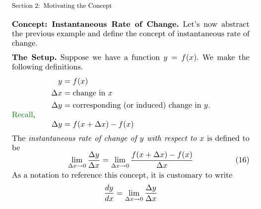
Concept: Instantaneous Rate of Change. Let’s now abstractthe previous example and define the concept of instantaneous rate ofchange.

The Setup. Suppose we have a function y = f(x). We make thefollowing definitions.

y = f(x)∆x = change in x

∆y = corresponding (or induced) change in y.Recall,

∆y = f(x+ ∆x)− f(x)

The instantaneous rate of change of y with respect to x is defined tobe

lim∆x→0

∆y∆x

= lim∆x→0

f(x+ ∆x)− f(x)∆x

(16)

As a notation to reference this concept, it is customary to write

dy

dx= lim

∆x→0

∆y∆x


Thus,

dy

dx= The (instantaneous) rate of change of y per unit

change in x.

In Example 2.5 we had V = 43πr

3 and we argued that

dV

dr= 4πr2.

This is a measure of the rate at which the volume, V , changes withrespect to (unit change in) r.

Solutions to Exercises

2.2. Obvious. Exercise 2.2.

Solutions to Exercises (continued)

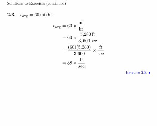
2.3. vavg = 60 mi/hr.

vavg = 60× mihr

= 60× 5,280 ft3, 600 sec

=(60)(5,280)

3,600× ft

sec

= 88× ftsec

Exercise 2.3.


2.4. Since h < 0, t0 + h < t0. Now at time t = t0 + h, the particle islocated at a = f(t0 + h), and at the later time of t = t0, the particleis located at b = f(t0). Now utilizing formulate (5) we get

vavg =f(t0)− f(t0 + h)t0 − (t0 + h)

=f(t0)− f(t0 + h)

−h=f(t0 + h)− f(t0)

h

Thus,

vavg =f(t0 + h)− f(t0)

h

Note that this expression is exactly the same as (9)! Consequently, inthe definition of instantaneous velocity given in equation (11).

Exercise 2.4.


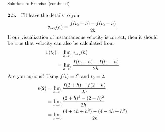
2.5. I’ll leave the details to you:

vavg(h) =f(t0 + h)− f(t0 − h)

2h.

If our visualization of instantaneous velocity is correct, then it shouldbe true that velocity can also be calculated from

v(t0) = limh→0

vavg(h)

= limh→0

f(t0 + h)− f(t0 − h)2h

Are you curious? Using f(t) = t2 and t0 = 2.

v(2) = limh→0

f(2 + h)− f(2− h)2h

= limh→0

(2 + h)2 − (2− h)2

2h

= limh→0

(4 + 4h+ h2)− (4− 4h+ h2)2h


= limh→0

8h2h

= limh→0

4

Now what do you suppose the last limit is? Try v(2) = 4 . . . as before!Can you think of other ways of covering t0 with different type timeintervals? Exercise 2.5.

2.6. As before,

msec(h) =√

4 + h− 2h

.

The above will be the basis for our calculations below.

msec = (√

4 + h− 2)/hh −1.0 −0.5 −0.1 −0.05 −0.01 −0.005 −0.001

msec .2679 .2583 .2516 .2508 .2502 .2501 .2500

What does the slope of the line tangent to the graph of f(x) =√x at

a = 4 appear to be? Again, it appears to be 0.25. Exercise 2.6.

Solutions to Examples

2.2. In this case f(x) =√x, f(4) = 2. If h > 0, then f(a + h) =

f(4 + h) =√

2 + h. Thus, from equation (12),

msec(h) =√

4 + h− 2h

.

The above will be the basis for our calculations below.

msec = (√

4 + h− 2)/hh 1.0 0.5 0.1 0.05 0.01 0.005 0.001

msec .2361 .2427 .2486 .2492 .2498 .2499 .2499

What does the slope of the line tangent to the graph of f(x) =√x at

a = 4 appear to be? Maybe 0.25, or there about? Example 2.2.

Solutions to Examples (continued)

2.3. We have y = f(x) = x2. If we increment (decrement) x a littleto get x + ∆x, then the value of y will be changed to another value,symbolically written as y + ∆y. From (14), we have

y = f(x) = x2

y + ∆y = f(x+ ∆x) = (x+ ∆x)2

= x2 + 2x∆x+ (∆x)2.Thus,

∆y = (y + ∆y)− y= (x2 + 2x∆x+ (∆x)2)− x2

= x2 + 2x∆x,and so,

∆y = 2x∆x+ (∆x)2.

If we change x by an amount of ∆x, then y changes by an amountof ∆y = 2x∆x + (∆x)2. (Note that the amount of change in the y-variable, ∆y, depends on both the value of x and the value of ∆x, theamount that the x is changed. This is typical.)


In numerical terms, let’s take x = 2. If we increase x = 2 by an amountof ∆x = .1, then the induced change in y is ∆y = 2(2)(.1) + (.1)2 =0.41. A change of ∆x = .1 gets, in this case, magnified to a change of∆y = .41.

Note that the induced change in y (that’s ∆y) depends not only onthe amount of change in the x (that’s ∆x), but also on the x-valueitself. For example,

For ∆x = .1x = 0 ∆y = .01x = 1 ∆y = .21x = 2 ∆y = .41x = 3 ∆y = .61

In all cases above, if we increase the value of x by ∆x = .1, thecorresponding value of y also increases (since ∆y > 0). We can also


get a negative ∆y. In the table below, ∆x = −.1, i.e. we decrementthe value of x by .1.

For ∆x = −.1x = 0 ∆y = 0.01x = 1 ∆y = −.19x = 2 ∆y = −.39x = 3 ∆y = −.59

Thus, decrementing the value of x also decrements the value of y —except for the case x = 0. Draw the graph of y = x2 to visualize whatis going on.

Example 2.3.


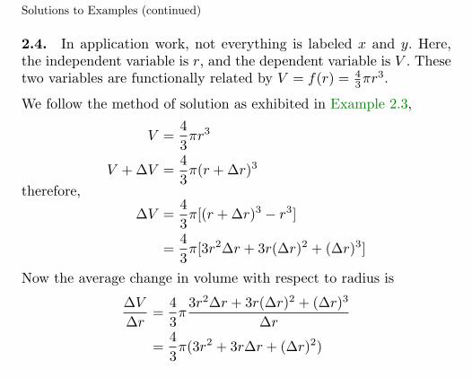
2.4. In application work, not everything is labeled x and y. Here,the independent variable is r, and the dependent variable is V . Thesetwo variables are functionally related by V = f(r) = 4

3πr3.

We follow the method of solution as exhibited in Example 2.3,

V =43πr3

V + ∆V =43π(r + ∆r)3

therefore,

∆V =43π[(r + ∆r)3 − r3]

=43π[3r2∆r + 3r(∆r)2 + (∆r)3]

Now the average change in volume with respect to radius is

∆V∆r

=43π

3r2∆r + 3r(∆r)2 + (∆r)3

∆r

=43π(3r2 + 3r∆r + (∆r)2)


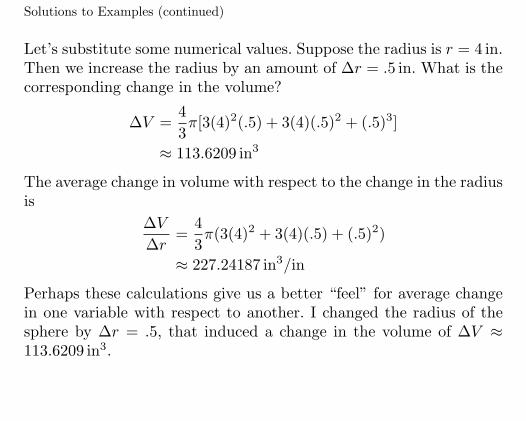
Let’s substitute some numerical values. Suppose the radius is r = 4 in.Then we increase the radius by an amount of ∆r = .5 in. What is thecorresponding change in the volume?

∆V =43π[3(4)2(.5) + 3(4)(.5)2 + (.5)3]

≈ 113.6209 in3

The average change in volume with respect to the change in the radiusis

∆V∆r

=43π(3(4)2 + 3(4)(.5) + (.5)2)

≈ 227.24187 in3/in

Perhaps these calculations give us a better “feel” for average changein one variable with respect to another. I changed the radius of thesphere by ∆r = .5, that induced a change in the volume of ∆V ≈113.6209 in3.


Now, what is the interpretation of ∆V/∆r? It represents the amountof change in the volume per unit change in r. To see this interpreta-tion, we bring forth the following analogy: Suppose you are movingat a rate of 30 mi each half-hour (.5 hour), how many miles are youmoving per unit hour? The answer:

v =30 mi.5 hr

= 60 mi/hr.

In a similar fashion we can interpret ∆V/∆r; indeed, the inclusion ofthe units of measurement suggest the interpretation:

∆V∆r≈ 227.24187 in3/in.

Thus the volume is changing at a (average) rate of 227.24187 in3 perinch; or, more exactly, when the radius was changed from r = 4 tor = 4.5 (that’s a change of ∆r = .5) the volume changed at a rateconsistent with 227.24187 in3 rate. Think about it!

Example 2.4.


2.5. Let us summarize the general results from Example 2.4.

V =43πr3

V + ∆V =43π(r + ∆r)3

∆V =43π[3r2∆r + 3r(∆r)2 + (∆r)3]

and,∆V∆r

=43π(3r2 + 3r∆r + (∆r)2) (S-0)

Now, ∆V/∆r represents the (average) change in volume per unitchange in r. What happens to ∆V/∆r as ∆r gets closer and closerto 0? That is, as we change the radius less and less, what affect doesthat have on the (average) change in volume per unit change in r?Can you see in equation (S-0), that if ∆r ≈ 0, then ∆V/∆r ≈ 4πr2?

We are interested in the behavior of ∆V/∆r as ∆r get closer and closerto 0 — this is the Pedestrian description of limit. Define instantaneousrate of change of V with respect to (unit changes in) x as

lim∆r→0

∆V∆r

= lim∆r→0

43π(3r2 + 3r∆r + (∆r)2)

=43π3r2

= 4πr2.

The quantity, 4πr2 represents the instantaneous rate of change ofvolume, V , with respect to unit change in x. For example, when theradius is r = 4, how fast is the volume changing? The answer

rate = 4π(4)2 = 64π ≈ 201.0618 in3/in.

When r = 4, volume can change at a rate of 201.0618 cubic inches,per inch change in the radius.

Example 2.5.

Index

Index

All page numbers are hypertextlinked to the corresponding topic.

Underlined page numbers indicate ajump to an exterior file.

Page numbers in boldface indicatethe definitive source of informationabout the item.

average velocity, c1l:2

constant velocity, c1l:1

continuous function, c1l:18

Euclid, c1l:12

limit, c1l:4limits

left-hand, c1l:42one-sided, c1l:41right-hand, c1l:44

Mathematical Induction, c1l:15

secant line, c1l:13, c1l:14

tangent line, c1l:13

2.2. instantaneous velocity toc assuming that your …dpstory/tutorial/c1/c1l_t1.pdfsection 2:...

Documents