22. introduction to formal verificationjaa/lectures/22-1.pdfformal veri cation approaches theorem...

22. Introduction to Formal Verification

Jacob Abraham

Department of Electrical and Computer EngineeringThe University of Texas at Austin

VLSI DesignFall 2017

November 20, 2017

ECE Department, University of Texas at Austin Lecture 22. Introduction to Formal Verification Jacob Abraham, November 20, 2017 1 / 48

Verification in the Design Cycle

Implementation Verification: Forall feasible inputs the behavior ofthe circuit is consistent with thebehavior required by thespecification

Design Verification: For allfeasible inputs the design has anumber of properties required bythe specification

Current formal verification techniques focused on functionalverification


Formal Verification Approaches

Theorem Proving: Relationship between a specification andan implementation is regarded as a theorem in a logic, to beproved within the framework of a proof calculus

Used for verifying arithmetic circuits in industry

Model Checking: The specification is in the form of a logicformula, the truth of which is determined with respect to asemantic model provided by an implementation

Starting to be used to check small modules in industry

Equivalence Checking: The equivalence of a specification andan implementation checked

Most common industry use of formal verification

Symbolic Trajectory Evaluation: Properties specified asassertions about circuit state (pre- and post- conditions),verified using symbolic simulation

Used to verify embedded memories in industry


Equivalence Checking

Most common technique of formal verification used inindustry today

Typically, gate-level compared with RTL

Canonical representations, such as Binary Decision Diagrams(BDDs), or Satisfiability Solvers used for the comparison

Boolean equivalence checking is NP-completeMultipliers require an exponential number of BDD nodes

Commercial tools available from many vendors


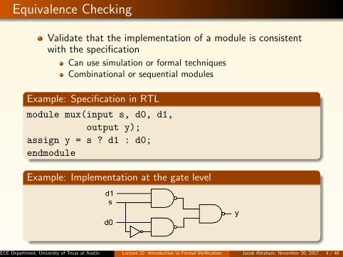
Equivalence Checking

Validate that the implementation of a module is consistentwith the specification

Can use simulation or formal techniquesCombinational or sequential modules

Example: Specification in RTL

module mux(input s, d0, d1,

output y);

assign y = s ? d1 : d0;

endmodule

Example: Implementation at the gate level


Decision Tree for A⊕B ⊕ C


Reduced, Ordered BDD (ROBDD)

F = A⊕B ⊕ C

Reduced, Ordered BDDs (ROBDDs) are canonical

Can represent sets of states, state-transition relations, etc.

Structure and complexity of ROBDDs for Symmetric Functions?ECE Department, University of Texas at Austin Lecture 22. Introduction to Formal Verification Jacob Abraham, November 20, 2017 6 / 48

Example of ROBDD Reduction


Impact of BDD Variable Orderingf(x1, x2, . . . , x8) = x1 · x2 + x3 · x4 + x5 · x6 + x7 · x8

Ordering : x1 < x3 < x5 < x7 < x2 < x4 < x6 < x8


Figure modified from Wikipedia

Impact of BDD Variable Ordering, Cont’df(x1, x2, . . . , x8) = x1 · x2 + x3 · x4 + x5 · x6 + x7 · x8

Ordering : x1 < x2 < x3 < x4 < x5 < x6 < x7 < x8


Figure modified from Wikipedia

Variable Swapping – An example


Probabilistic Verification

Concept of arithmetic simulation

Transform Boolean function or circuit so that operationsperformed on arithmetic (rather than Boolean) variables

Evaluate specification and implementation for a randomarithmetic vector (result called a hash code)

If hash codes are different, the two are definitely notequivalentIf hash codes are the same, there is a small probability of error(that is, the two may not be equivalent)

error e = 1m , where m is the size of the integer space

Probability of error can be reduced by using integers from alarger space, or by repeating evaluation on another randomvector (error decreases exponentially)

The error after k runs, e = ( 1m)k

Example probability of error for 32-bit integers: 10−8

Each evaluation reduces error by the above factor


Indexed Binary Decision Diagrams

A BDD graph with multiple layersCharacteristics:

function graph is divided into k layerseach layer is strongly orderedtwo layers can have different orderingExample: F = (a1 ⊕ a2 ∨ a3 ⊕ a4) ∧ (a1 ⊕ a3 ∨ a2 ⊕ a4)


Satisfiability (SAT) Solvers

Can a Boolean Function be Satisfied?

Cast an equivalence checking problem as a SAT problem

Starts by converting Boolean formula into the ConjunctiveNormal Form (CNF) – (product of sums)

(a+ b+ c)(a+ e+ f)(c+ d+ g). . .

Goal is to find an assignment satisfying every term (if anyclause is 0, there is no satisfying assignment)

Commercial and Open SAT solvers available

Most verification tools now use BDDs + SAT

Some bring in ATPG ideas – called “structural SAT”


Truth Table to CNF

Put negation of formula in DNF

For each “0” or “F” row in table, make a term equivalent tothe corresponding assignment

Negate the disjunction of the terms

By DeMorgan’s Law, switch AND and OR, and complementliterals

Example: Express x↔ y (x · y + x · y) in CNF

Two terms for “0”: x=1, y=0 and x=0, y=1=⇒ function is “0” when xy + xy

CNF is: (x+ y)(x+ y)


Circuit to CNF

d ≡ (a+ b)

Clauses:(a+ b+ d)(a+ d)(b+ d)

e ≡ (c.d)

Clauses:(c+ d+ e)(d+ e)(c+ e)


Use of ATPG for Equivalence Checking

Use a tool (Automatic Test Pattern Generator) whichgenerates manufacturing tests

Detecting a “stuck-at-0” fault at Y (requires an input whichgenerates a 1 on Y) will prove inequivalence of the two circuits

Approach is not memory limited (like BDDs)


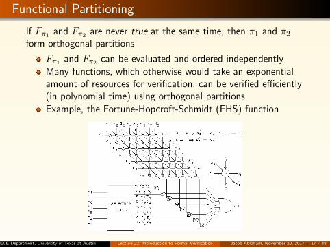
Functional Partitioning

If Fπ1 and Fπ2 are never true at the same time, then π1 and π2form orthogonal partitions

Fπ1 and Fπ2 can be evaluated and ordered independently

Many functions, which otherwise would take an exponentialamount of resources for verification, can be verified efficiently(in polynomial time) using orthogonal partitions

Example, the Fortune-Hopcroft-Schmidt (FHS) function


Term Rewriting for Arithmetic Circuit Checking

RTL Term-Level reductions

Verification of arithmetic circuits at the RTL level using termrewriting

RTL to RTL equivalence checking

Verified large multiplier designs like Booth, Wallace Tree andmany optimized multipliers using this rewriting technique

VERIFIRE

Dedicated Arithmetic Circuit Checker

Vtrans: Translates Verilog designs to Term Rewriting Systems

Vprover: Proves equivalence of Term Rewriting Systems

Iterative engineReturns error trace if proof not foundMaintains an expanding rule base for expression minimizationIncomplete, but efficient, engine


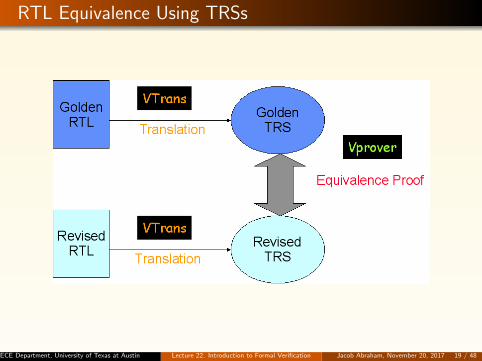
RTL Equivalence Using TRSs


Results on Multipliers

Different sizes of Wallace Tree Multipliers (Verilog RTL) comparedwith a simple Golden Multiplier (Verilog RTL) of the same size

Compare Verifire against Commercial Tools

Wallace Tree Verifire Commercial Tool 1 Commercial Tool 2

4x4 14s 10s 9s

8x8 18s 18s 16s

16x16 25s unfinished unfinished




Application of Theorem Proving

ACL2 used at AMD to formally verify FPUs

First used by Moore et al. to check the proof of correctness ofthe Kernel of the AMD 5k86 floating point division algorithm

Used to verify the RTL of K7 FPU

RTL primitives logical operations on bit vectorsDeveloped theory to prove RTL correct with respect to moreabstract IEEE standard

Theorem proving requires high degree of expertise


Symbolic Simulation

Equivalence checking between RTL and circuit schematics isdifficult for some circuits (e.g., custom arrays)

Critical timing and self-timed control logicLarge number of bit-cellsInherently complex sequential logic blocksDynamic logic

Traditional tools fail on such circuits

Very large state space, too many initial state/input sequencesfor simulation-based toolsBoolean equivalence tools only check static cones of logic, donot capture dynamic behavior


Example: Custom Control for Custom Array Structures

OUT pulse fans out to array READ/WRITE control signals

Equivalence checking does not work


Scalar Simulation

To prove that the circuit is a NAND gate, exhaustive simulationrequires 2n vectors

Antecedent Consequent

A = 0 (t0,t1) and B = 0 (t0,t1) C is 1 (t1,t2)

A = 0 (t0,t1) and B = 1 (t0,t1) C is 1 (t1,t2)

A = 1 (t0,t1) and B = 0 (t0,t1) C is 1 (t1,t2)

A = 1 (t0,t1) and B = 1 (t0,t1) C is 0 (t1,t2)

Table could be viewed as: Antecedent =⇒ Consequent


Ternary Simulation

Using three values (0, 1, X), N-input NAND requires N+1 vectorsto verify

Antecedent Consequent

A = 0 (t0,t1) and B = X C is 1 (t1,t2)

A = X and B = 0 (t0,t1) C is 1 (t1,t2)

A = 1 (t0,t1) and B = 1 (t0,t1) C is 0 (t1,t2)


Symbolic Simulation

Exhaustive Verification: N-input NAND requires 1 vector and Nvariables

Antecedent: A = “a”(t0,t1) and B = “b”(t0,t1)(“a” and “b” are Boolean variables)

Consequent: C = [¬ (a AND b)](t1,t2)


Symbolic Trajectory Evaluation

VERSYS symbolic trajectory evaluation tool developed atMotorola/Freescale

Based on VOSS (from CMU/UBC)

Trajectory formulasBoolean expressions with the temporal next-time operatorTernary values states represented by a Boolean encoding

Properties of type: Antecedent =⇒ ConsequentAntecedent, Consequent are trajectory formulasAntecedent sets up stimulus, state of the circuitConsequent specifies constraint on the state sequence

Used to verify PowerPC arrays at Motorola/Freescale in 8 –10% of the design timeBugs found during array equivalence checking

Incorrect clock regenerators feeding latchesControl logic errors in READ/WRITE enablesViolation of “one-hot” property assumptionsScan chain hookup errorsPotential circuit-related problems such as glitches and races


Design Verification

Digital systems similar to reactive programsDigital systems receive inputs and produce outputs in acontinuous interaction with their environmentBehavior of digital systems is concurrent because each gate inthe system simultaneously evaluating its output as a functionof its inputs

Check Properties of Design

Since specification is usually not formal, check design forproperties that would be consistent with the specification

Safety “something bad will never happen”

Liveness Property: “something good will eventually happen”

Temporal Logic and variations commonly used to specifyproperties

Example: Linear Temporal Logic (LTL) or Computation TreeLogic (CTL)


Example of Computation Tree

Traffic light controller


Operators

Referring to pathsA: For every pathE: There exists a path

Referring to states on a pathG: GloballyF: In the future (eventually)

ExamplesEF p: there is some path on which p is eventually trueAG p: for every path, at every state, p is true


EG R (True)EF Y (True)

AG(R+G) (False)

Use of ATPG to Check Properties

This moves verification of the design to the same level as themodels used to generate manufacturing test of the physicalchip

Using ATPG allows the verification engine to deal withtri-state signals, multiple clocks, etc.

Bounded Model Checking: Prove properties for a limited numberof cycles


Monitor State Machine for EGp

Find an input sequence of length n for which the system willsatisfy the property p


Monitor State Machine for EpUq

For some path of up to n cycles, there is a state where q holds andp holds in every previous state


Model Checking on IBM Power 4

“Functional formal verification” (equivalence checking andmodel checking) on ≈40 design components (IU, FPU,control, memory, etc.)

Found more than 200 design flaws at various stages and ofvarying complexity

At least one bug was found by almost every application offormal verification

Estimate: 15% of bugs would have evaded simulation

Some of the bugs literally escaped 1-2 years of simulation


Specifying Properties (Assertions) in Industry Tools

Used for both simulation monitoring and formal verification

Examples of assertion languages include Vera (Synopsys),Sugar (IBM), Property Specification Language,PSL (Acceleraconsortium), System Verilog

PSL/Sugar

Core based on Boolean and Temporal logic

Layer of user-friendly “syntactic sugar”

Comes in three flavors

VerilogVHDLGDL

Reference Manual:http://www.eda.org/vfv/docs/PSL-v1.1.pdf


http://www.eda.org/vfv/docs/PSL-v1.1.pdf

System Verilog Assertions (SVA)

SVA

Assertions: Predicates placed in program

Immediate and Concurrent Assertions

assert, assume, cover, expect constructs

Immediate Assertions

assert (a == b);

Concurrent Assertions

assert property (@(posedge clk) req | → ack);


Cadence Formal Verification


Dealing with State Explosion

Verification is a very difficult problem

Even combinational equivalence checking problems (ATPG,SAT) are NP-complete

Checking sequential properties is only possible for smalldesigns

Additional problem of generating correct “wrappers” for themodule being verified

How can we deal with the complexity?

Use more powerful computers?

Computers double in capability (assuming we can programmulti-core processors) every couple of yearsAdding one state variable to a design doubles its states

Exploit hierarchy in the design

Develop powerful abstractions


Program Slicing

A Slice of a Design

Represents behavior of the design with respect to a given setof variables (or slicing criterion)

Proposed for use in software in 1984 (Weiser)

Slice generated by a control/data flow analysis of the programcode

Slicing is done on the structure of the design, so scales well

“Static analysis”


Antecedent Conditioned Slicing


Example of Antecedent Conditioned Slicing – I


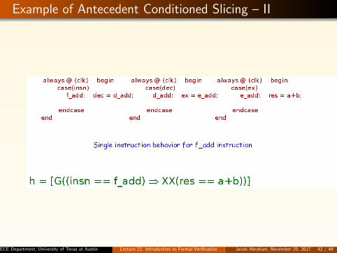
Example of Antecedent Conditioned Slicing – II


Experiments with Antecedent Conditioned Slicing

USB 2.0 Function Core

Verilog implementation from www.opencores.org

Properties from specification document

Safety properties expressed in LTL (G(a =⇒ c))

Verification engine: Cadence-BMC (bound of 24–50 steps)


Example USB Properties

G((crc5err ∨ ¬(match) =⇒ ¬(send token))If a packet with a bad CRC5 is received, or there is an endpointfield mismatch, the token is ignored

G((state == SPEED NEG FS) =⇒ X((mode hs) ∧(T1 gt 3 0ms) =⇒ (next state == RES SUSPEND))

If the machine is in the speed negotiation state, then in the nextclock cycle, if it is in high speed mode for more than 3 ms, it willgo to the suspend state

G((state == RESUME WAIT ) ∧ ¬(idle cnt clr) =⇒F (state == NORMAL))

If the machine is waiting to resume operation and a counter is set,eventually (after 100 mS) it will return to normal operation


Results on Temporal USB Properties

CPU seconds, on a 450 MHz dual UltraSPARC-II with I GB RAM


Verification of Processors Using Antecedent ConditionedSlicing

Verification of single-instruction issue, multi-stage pipelinedprocessors

Properties are at the Instruction level (not for an internalblock in the design)

Antecedent conditioned slicing provides an automaticdecomposition strategy

Individual “instruction machines”

Verified all the instructions of the OR1200 embeddedprocessor (www.opencores.org)


Single Instruction Verification


Results of OR1200 Verification

CPU seconds, 3GHz Pentium 4 processor with 1 GB RAM

SMV would not even compile the design without slicing

Instruction Instruction SMV time Memory UsageClass (seconds) (KB)

LSU l.ld 35.85 29104

LSU l.lws 33.91 28873

LSU l.sd 38.32 30941

SHF/ROT l.sll 26.81 23771

SHF/ROT l.srl 27.83 23771

SHF/ROT l.ror 27.83 26919

SPRS l.mfspr 226.97 50696

SPRS l.mtspr 212.27 48627


22. introduction to formal verificationjaa/lectures/22-1.pdfformal veri cation approaches theorem...

Documents