Stochastic Control !Robert Stengel!

Robotics and Intelligent Systems, MAE 345, Princeton University, 2017

•! Markov Process•! Overview of the Linear-Quadratic-Gaussian

(LQG) Regulator•! Introduction to Stochastic Robust Control Laws

Copyright 2017 by Robert Stengel. All rights reserved. For educational use only.http://www.princeton.edu/~stengel/MAE345.html

Learning Objectives

1

Deterministic vs. Stochastic Optimal Control

•! Deterministic control–! Known dynamic process

•! precise input•! precise initial condition•! precise measurement

–! Optimal control minimizes J* = J(x*, u*)

•! Stochastic control–! Known dynamic process

•! unknown input•! imprecise initial condition•! imprecise or incomplete measurement

–! Optimal control minimizes E{J[x*, u*]}

2

z(t) = Hx(t)+ n(t)!x(t) = F(t)x(t)+G(t)u(t)+K(t) z(t)!Hx(t)[ ]u(t) = !C(t) x(t)+ ucommand

Linear-Quadratic-Gaussian (LQG) Control of a Dynamic Process

!

3

Linear-Quadratic (LQ) Control Equations (Continuous-Time Model)

!x t( ) = Fx(t)+Gu t( )

u t( ) = !Cx(t)+ ucommand

Open-Loop System State Dynamics

Control Law

4

!x t( ) = F !GC( )x(t)+GCucommandCharacteristic Equation

sI! F !GC( ) = 0How many eigenvalues? Stable or unstable?

n Stable, with correct design criteria, F, and G

Closed-Loop System State Dynamics

Linear-Quadratic-Gaussian (LQG) Control Equations

(Continuous-Time Model)

!x t( ) = Fx(t)+Gu(t)+Lw(t)z t( ) = Hx t( ) + n t( )

u t( ) = !Cx(t)+ ucommand

!x t( ) = Fx(t)+Gu(t)+K z t( )!Hx t( )"# $%

Open-Loop System State Dynamics and Measurement

Control Law

State Estimate

5

Linear-Quadratic-Gaussian (LQG) Control Equations

(Continuous-Time Model)

!x t( ) = Fx(t)+G !Cx(t)[ ]+Lw(t)

!x t( ) = Fx(t)+G !Cx(t)[ ]+K z t( )!Hx t( )"# $%

6

Closed-Loop System State and Estimate Dynamics (neglect command)

How many eigenvalues?

Stable or unstable?

2n

TBD

LQG Separation PropertyOptimal estimation algorithm does not depend on the

optimal control algorithm

K t( ) = P(t)HTN!1 t( )!P(t) = F(t)P(t)+ P(t)FT (t)+L t( )W t( )LT t( )! P(t)HTN!1 t( )HP(t)

Optimal control algorithm does not depend on the optimal estimation algorithm

C t( ) = R!1 t( )GT t( )S t( )!S t( ) = !Q(t)! F(t)T S t( )! S t( )F(t)+ S t( )G(t)R!1(t)GT (t)S t( )

7

LQG Certainty Equivalence

Stochastic feedback control law is the same as the deterministic control law

Stochastic feedback control is computed from optimal estimate of the state

u*(t) = !R!1GT (t)S(t)x(t) = !C(t) x(t)

u*(t) = !R!1GT (t)S(t)x(t) = !C(t) x(t)

8

Asymptotic Stability of the LQG Regulator !

(with no parameter uncertainty)!

9

System Equations with Continuous-Time LQG Control

!! t( ) ! x t( )" x t( )

!!! t( ) = F "KH( )!! t( ) + Lw t( ) "Kn t( )

With perfect knowledge of the system

State estimate error

State estimate error dynamics

10

!x t( ) = Fx(t)+G !Cx(t)[ ]+Lw(t)

!x t( ) = Fx(t)+G !Cx(t)[ ]+K z t( )!Hx t( )"# $%

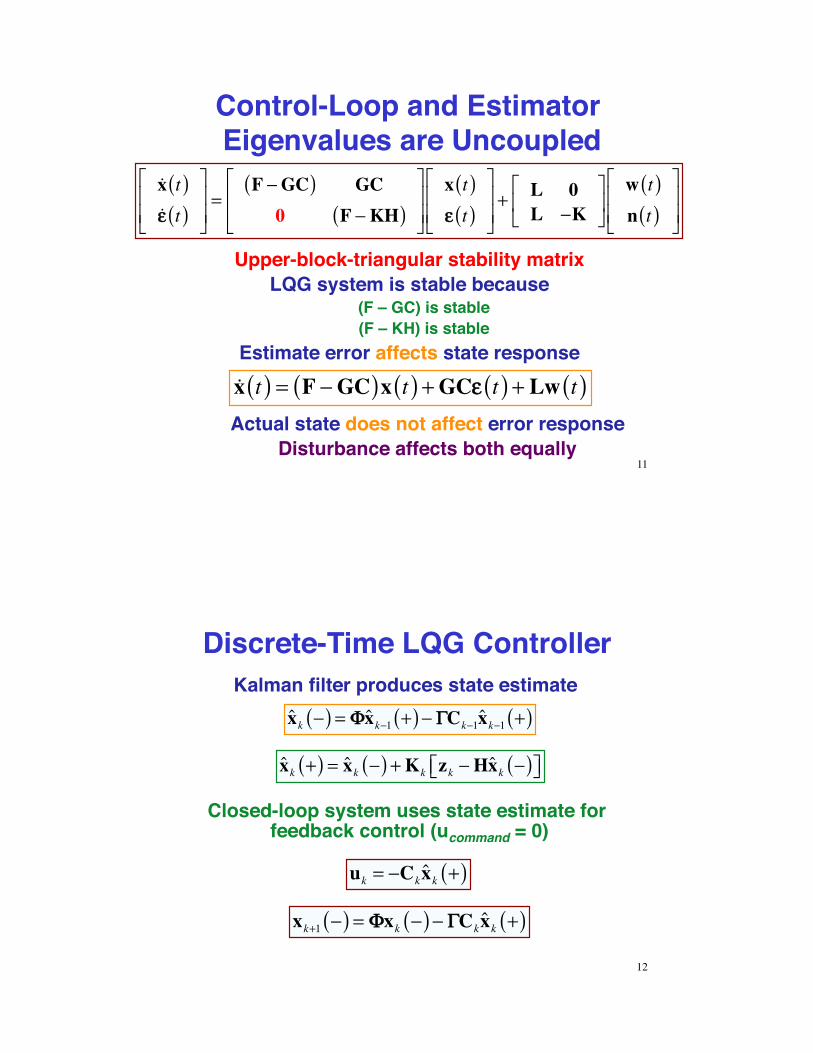
Control-Loop and Estimator Eigenvalues are Uncoupled

!x t( )!!! t( )

"

#$$

%

&''=

F (GC( ) GC0 F (KH( )

"

#$$

%

&''

x t( )!! t( )

"

#$$

%

&''+ L 0

L (K"

#$

%

&'w t( )n t( )

"

#$$

%

&''

Upper-block-triangular stability matrixLQG system is stable because

(F – GC) is stable(F – KH) is stable

Estimate error affects state response

Actual state does not affect error responseDisturbance affects both equally

!x t( ) = F !GC( )x t( ) +GC"" t( ) + Lw t( )

11

Discrete-Time LQG ControllerKalman filter produces state estimate

xk !( ) = ""xk!1 +( )! ##Ck!1xk!1 +( )

uk = !Ckxk +( )

xk +( ) = xk !( ) +Kk zk !Hxk !( )"# $%

Closed-loop system uses state estimate for feedback control (ucommand = 0)

xk+1 !( ) = ""xk !( )! ##Ckxk +( )

12

Response of Discrete-Time 1st-Order System to Disturbance, and

Kalman Filter Estimate from Noisy Measurement

Propagation of Uncertainty Kalman Filter, Uncontrolled System

13

Comparison of 1st-Order Discrete-Time LQ and LQG Control Response

Linear-Quadratic Control with Noise-free Measurement

Linear-Quadratic-Gaussian Control with Noisy Measurement

14

MATLAB Demo: LQG Rolling Mill Control System Design Example

•! Maintain desired thickness of shaped beam

•! Account for random–! variations in thickness/

hardness of incoming beam–! eccentricity in rolling cylinders–! measurement errors

Open- and Closed-Loop Response

http://www.mathworks.com/help/control/ug/lqg-regulation-rolling-mill-example.html15

Robust Stochastic Control!

16

•! Stochastic controller •! minimize response to random initial conditions, disturbances,

and measurement errors•! perfect knowledge of the plant

•! Robust controller •! fixed gains and structure•! minimize likelihood of instability or unsatisfactory performance

due to parameter uncertainty in the plant•! Adaptive controller

•! variable gains and/or structure•! minimize likelihood of instability or unsatisfactory performance

due to plant parameter uncertainty, disturbances, and measurement errors

Stochastic, Robust, and Adaptive Control

Practical controller may have elements of all three17

Robust Control System Design•! Make closed-loop response insensitive to plant

parameter variations•! Robust controller

–! Fixed gains and structure–! Minimize likelihood of instability–! Minimize likelihood of unsatisfactory performance

18

Probabilistic Robust Control Design

•! Design a fixed-parameter controller for stochastic robustness

•! Monte Carlo Evaluation of competing designs•! Genetic Algorithm or Simulated Annealing

search for best design

19

Representations of Uncertainty

sI! F = det sI! F( ) !"(s) = sn + an!1s

n!1 + ...+ a1s + a0= s ! #1( ) s ! #2( ) ...( ) s ! #n( ) = 0

Characteristic equation of the uncontrolled system

•! Uncertainty can be expressed in–! Elements of F–! Coefficients of "(s)–! Eigenvalues of F

20

Root Locations for an Uncertain 2nd-Order System

•! Variation may be represented by–! Worst-case, e.g., Upper/lower bounds of uniform distribution–! Probability, e.g., Gaussian distribution

Uniform Distribution Gaussian Distribution

s Plane s Plane

21

“3-D” Stochastic Root Loci for 2nd-Order Example

•! Root distributions are nonlinear functions of parameter distributions

•! Unbounded parameter distributions always lead to non-zero probability of instability

•! Bounded distributions may be guaranteed to be stable

22

Probability of Satisfying a Design Metric

•! Probability of satisfying a design metric–! d: Control design parameter vector [e.g., SA, GA, …]–! v: Uncertain plant parameter vector [e.g., RNG]–! e: Binary indicator, e.g., ! 0: satisfactory 1: unsatisfactory–! H(v): Plant –! C(d): Controller (Compensator)

Pr(d,v) ! 1N

e C d( ),H v( )"# $%i=1

N

&

23

Design Control System to Minimize Probability of Instability

!closed"loop (s) = sI" F v( )"G v( )C d( )#$ %&= s " '1( ) s " '2( ) ...( ) s " 'n( )#$ %&closed"loop = 0

•! Characteristic equation of the closed-loop system

•! Monte Carlo evaluation of probability of instability with uncertain plant parameters

•! Minimize probability of instability using numerical search of control parameters

mind

Pr Re !i , i = 1,n( )"# $% > 0{ }24

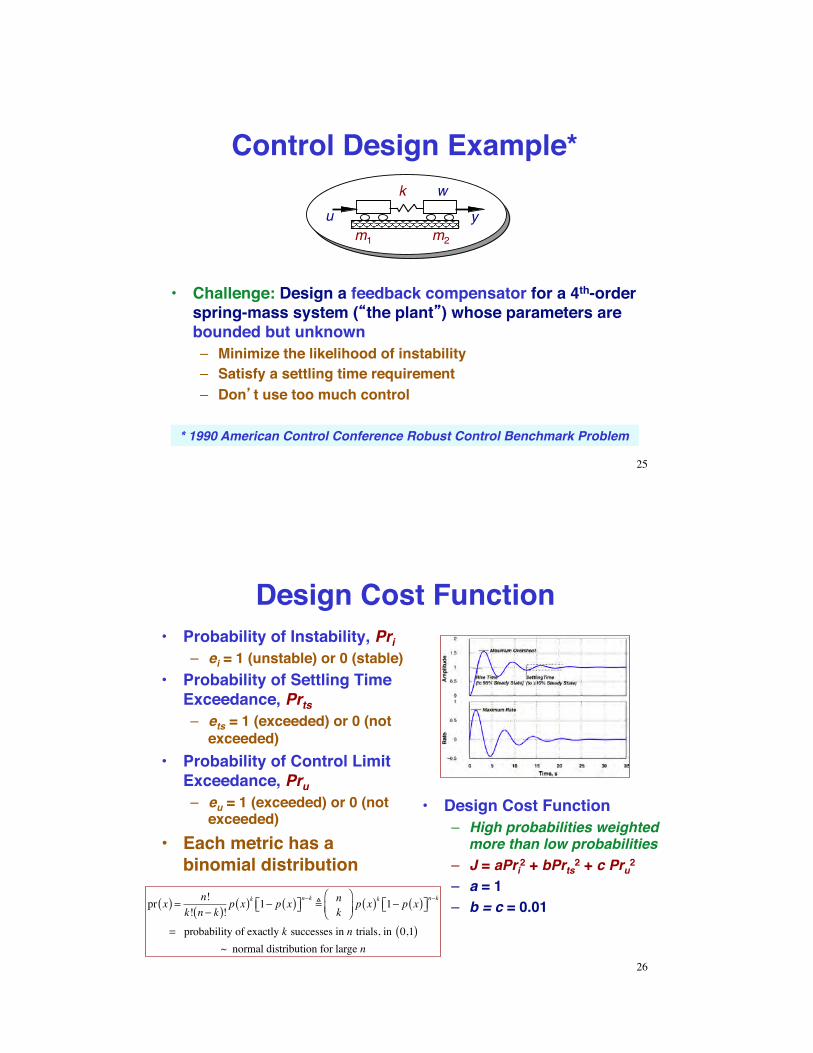
Control Design Example*

•! Challenge: Design a feedback compensator for a 4th-order spring-mass system ( the plant ) whose parameters are bounded but unknown–! Minimize the likelihood of instability–! Satisfy a settling time requirement–! Don t use too much control

* 1990 American Control Conference Robust Control Benchmark Problem

m1 m2

ku y

w

25

Design Cost Function •! Probability of Instability, Pri

–! ei = 1 (unstable) or 0 (stable)•! Probability of Settling Time

Exceedance, Prts –! ets = 1 (exceeded) or 0 (not

exceeded)•! Probability of Control Limit

Exceedance, Pru –! eu = 1 (exceeded) or 0 (not

exceeded)•! Each metric has a

binomial distribution

•! Design Cost Function–! High probabilities weighted

more than low probabilities–! J = aPri

2 + bPrts2 + c Pru

2 –! a = 1–! b = c = 0.01

pr x( ) = n!k! n ! k( )! p x( )k 1! p x( )"# $%

n!k! n

k&'(

)*+p x( )k 1! p x( )"# $%

n!k

= probability of exactly k successes in n trials, in 0,1( )~ normal distribution for large n

26

Monte Carlo Evaluation of Probability of Satisfying a Design Metric

1e+01

1e+03

1e+05

1e+07

1e+09

1e-06 1e-05 1e-04 0.001 0.01 0.1 1

2%5%10%20%

100%

Num

ber

of E

valu

atio

ns

0.5

IntervalWidth

Probability or (1 - ProbabilityBinomial Distribution

•! Compute v using random number generators over N trials–! Required number of trials

depends on outcome probability and desired confidence interval

•! Search for best d using a genetic algorithm to minimize J

Prk (d,v) !1N

ek C d( ),H v( )"# $%i=1

N

& , k = 1,3

J = aPri2 (d,v)+ bPrts

2 (d,v)+ cPru2 (d,v)

27

Uncertain Plant*

Plant dynamic equation

* 1990 American Control Conference Robust Control Benchmark Problem

m1 m2

ku y

!x1!x2!x3!x4

!

"

#####

$

%

&&&&&

=

0 0 1 00 0 0 1

' k m1 k m1 0 0k m2 ' k m2 0 0

!

"

#####

$

%

&&&&&

x1x2x3x4

!

"

#####

$

%

&&&&&

+

001 m1

0

!

"

####

$

%

&&&&

u +

000

1 m2

!

"

####

$

%

&&&&

w

w

!(s) = s2 s2 + km1 + m2( )m1m2

"

#$

%

&' = s2 s2 ()n

2"# %&

4th-Order Plant characteristic equation

y = x2 + n

28

Parameter Variations and Open-Loop Roots

•! Parameters of mass-spring system–! Uniform probability density

functions for •! 0.5 < m1, m2 < 1.5 •! 0.5 < –k < 2

•! Neutral stability for all mass-spring values

x

x

xx

!(s) = s2 s2 + km1 +m2( )m1m2

"

#$

%

&'

= s2 s2 () n2"# %&

29

Mass-Spring-Mass Stabilization Requires Compensation

•! Proportional feedback alone cannot stabilize the system

•! Feedback of either sign drives at least one root into the right half plane

u s( ) = !cy s( ) ! !cx2 s( )

30

c ! 0, Blue locus of rootsc " 0, Green locus of roots

Single-input/single-output (SISO) feedback control law

x

xxx

Search-and-Sweep Design of Family of Robust SISO Feedback Compensators

Arrange parameters as binary design vector

C12 (s) =a0 + a1s

b0 + b1s + b2s2 ! C d( )

d = a0 ,a1,b0 ,b1,b2{ }

d* = a0*,a1*,b0*,b1*,b2 *{ }Search for design

vector, d, that minimizes J

Begin with lowest-order feedback compensator

m1 = rand 1( ) + 0.5m2 = rand 1( ) + 0.5k = !1.5*rand 1( ) + 0.5

Monte Carlo evaluation with

uncertain parameters, v31

Search-and-Sweep Design of Family of Robust Feedback Compensators

1)# Define next higher-order compensator

2)# Optimize over all parameters, including optimal coefficients in starting population

3)# Sweep to satisfactory design or no further improvement

C22 (s) =a0 + a1s + a2s

2

b0 + b1s + b2s2

d = a0*,a1*,a2,b0*,b1*,b2 *{ }! d**= a0 **,a1 **,a2 **,b0 **,b1 **,b2 **{ }

C23(s) =a0 + a1s + a2s

2

b0 + b1s + b2s2 + b3s

3 C33(s) =a0 + a1s + a2s

2 + a3s3

b0 + b1s + b2s2 + b3s

3

C34 (s) =a0 + a1s + a2s

2 + a3s3

b0 + b1s + b2s2 + b3s

3 + b4s4 ...

32

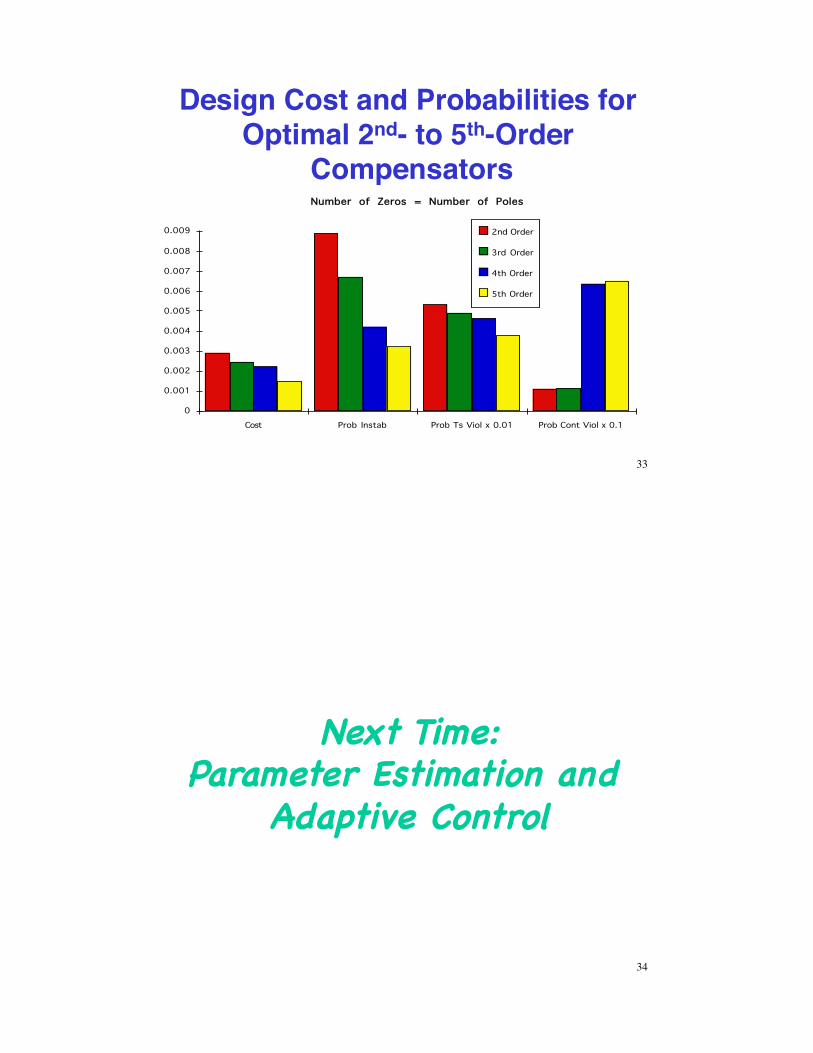
Design Cost and Probabilities for Optimal 2nd- to 5th-Order

CompensatorsNNuummbbeerr ooff ZZeerrooss == NNuummbbeerr ooff PPoolleess

0

0.001

0.002

0.003

0.004

0.005

0.006

0.007

0.008

0.009

Cost Prob Instab Prob Ts Viol x 0.01 Prob Cont Viol x 0.1

2nd Order

3rd Order

4th Order

5th Order

33

Next Time:!Parameter Estimation and

Adaptive Control!

34

SSuupppplleemmeennttaall MMaatteerriiaall

35

Example: Probability of Stable Control of an Unstable Plant

F =

!2gf11 /V "V 2 f12 / 2 "Vf13 !g

!45 /V 2 "Vf22 / 2 1 0

0 "V 2 f32 / 2 "Vf33 00 0 1 0

#

$

%%%%%

&

'

(((((

; G =

g11 g120 0g31 g320 0

#

$

%%%%%

&

'

(((((

; x =

V)q*

#

$

%%%%

&

'

((((

p = ! V f11 f12 f13 f22 f32 f33 g11 g12 g31 g32"#

$%T

!1"4 = "0.1± 0.057 j, " 5.15, 3.35

Longitudinal dynamics for a Forward-Swept-Wing Aircraft

Nominal eigenvalues (one unstable)

X-29 Aircraft

Environment Uncontrolled Dynamics Control Effect

Air density and airspeed, ! and V , have uniform distributions(±30%)10 coefficients have Gaussian distributions (! = 30%)

36

LQ Regulators for the Example

•! Case a) LQR with low control weighting

•! Case b) LQR with high control weighting

Q = diag 1,1,1,0( ); R = 1,1( ); !1"4nominal = –35,–5.1,–3.3,–.02

C = 0.17 130 33 0.360.98 "11 "3 "1.1

#

$%

&

'(

Q = diag 1,1,1,0( ); R = 1000,1000( ); !1"4nominal = "5.2,"3.4,"1.1,".02

C = 0.03 83 21 "0.060.01 "63 "16 "1.9

#

$%

&

'(

!1"4nominal = "32,–5.2,–3.4,–0.01

C = 0.13 413 105 "0.320.05 "313 "81 "1.1" 9.5

#

$%

&

'(

•! Case c) Case b with gains multiplied by 5 for bandwidth (loop-transfer) recovery

Three stabilizing 2-input feedback control laws

37

Stochastic Robustness !(Ray, Stengel, 1991)

"! Distribution of closed-loop roots with"! Gaussian uncertainty in 10 parameters"! Uniform uncertainty in velocity and air density

"! 25,000 Monte Carlo evaluations

Stochastic Root Locus

"! Probability of instability"! a) Pr = 0.072"! b) Pr = 0.021"! c) Pr = 0.0076

38

Probabilities of Instability for the Three Cases

39

Stochastic Root Loci for the Three Cases

Case a: Low LQ Control Weights

Case b: High LQ Control Weights

Case c: Bandwidth Recovery

with Gaussian Aerodynamic Uncertainty!

•! Probabilities of instability with 30% uniform aerodynamic uncertainty!–! Case a: 3.4 x 10-4!–! Case b: 0!–! Case c: 0!

40

Markov Process!

41

Markov Sequence and Process

"! Markov Process (Continuous Time)"! Probability distribution of dynamic process at

time s > t > 0, conditioned on the past history "! Depends only on the state, x, at time t

"! Markov Sequence (Discrete Time)"! Probability distribution of dynamic process at

time tk+1 > tk > 0, conditioned on the past history "! Depends only on the state, x, at time tk

Pr xk+1 | xk , xk!1, xk!2 ,!,0( )"# $% = Pr xk+1 | xk[ ]

42

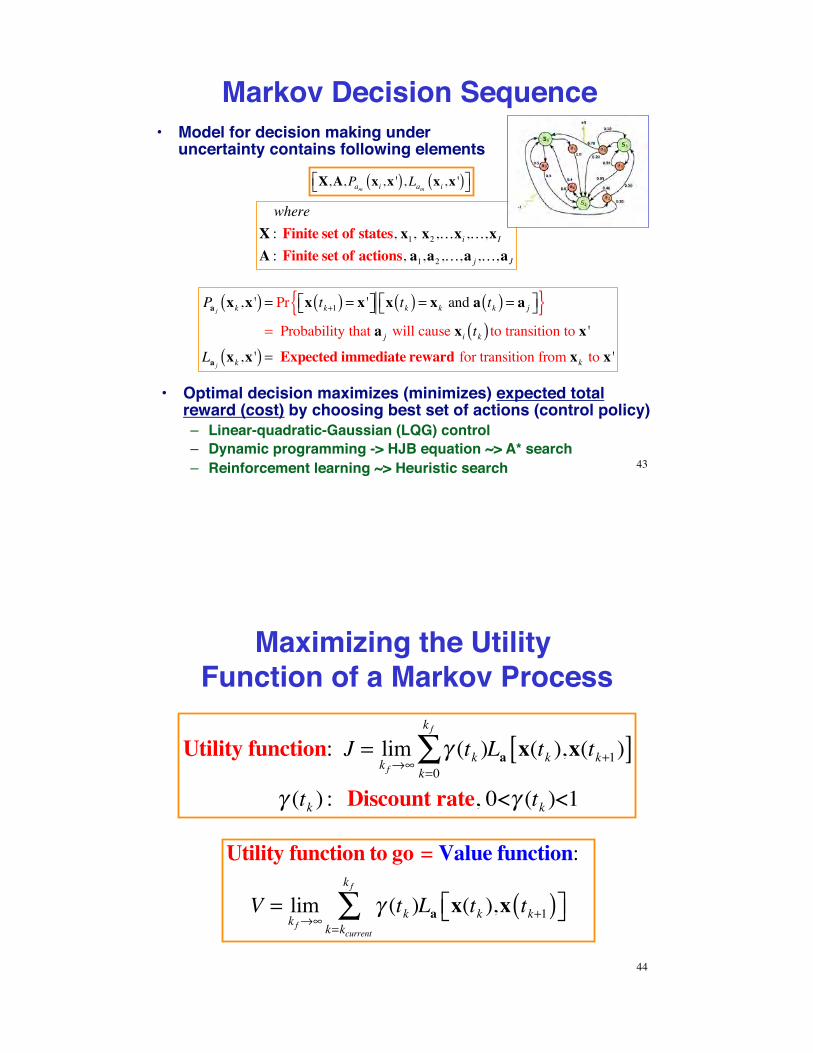
Markov Decision Sequence•! Model for decision making under

uncertainty contains following elements

X,A,Pam xi ,x '( ),Lam xi ,x '( )!" #$

•! Optimal decision maximizes (minimizes) expected total reward (cost) by choosing best set of actions (control policy)–! Linear-quadratic-Gaussian (LQG) control–! Dynamic programming -> HJB equation ~> A* search–! Reinforcement learning ~> Heuristic search

whereX : Finite set of states, x1, x2,…xi ,…,x I

A : Finite set of actions, a1,a2,…,a j ,…,aJ

43

Pa jxk ,x '( ) = Pr x tk+1( ) = x '!" #$ x tk( ) = xk and a tk( ) = a j!" #${ }

= Probability that a j will cause xi tk( ) to transition to x '

La jxk ,x '( ) = Expected immediate reward for transition from xk to x '

Maximizing the Utility Function of a Markov Process

Utility function: J = limk f!"

# (tk )k=0

k f

$ La x(tk ),x(tk+1)[ ]# (tk ) : Discount rate, 0<# (tk )<1

Utility function to go = Value function:

V = limk f!"

# (tk )k=kcurrent

k f

$ La x(tk ),x tk+1( )%& '(

44

Maximizing the Utility Function of a Markov Process

uopt tk( ) = argmaxa

La x(tk ),x(tk+1)[ ] + ! (tk ) Pa x(tk ),x(tk+1))[ ]V x(tk+1)[ ]k= kcurrent

"

#$%&

'&

()&

*&

Optimal control at t

Optimized value function

V * tk( ) = Luopt (tk ) x * (tk )[ ] + ! (tk ) Puopt (tk ) x * (tk ),xest * (tk+1)[ ]V x *est (tk+1)[ ]k= kcurrent

"

#

45

LQG Control Optimizes Discrete-Time LTI Markov Process

X,A,Pam xi ,x '( ),Lam xi ,x '( )!" #$

whereX : Finite set of states, x1, x2 ,…xi ,…,x I

A : Finite set of actions, a1,a2 ,…,a j ,…,aJ

Pa jxk ,x '( ) = Pr x tk+1( ) = x '!" #$ x tk( ) = xk and a tk( ) = a j!" #${ }

= Probability that a j will cause xi tk( ) to transition to x '

La jxk ,x '( ) = Expected immediate reward for transition from xk to x '

LQG Gain Calculation

46