2.2A INTRODUCTION TO NORMAL DISTRIBUTIONS

SECTION 2.2ANORMAL DISTRIBUTIONS

After this lesson, you should be able to…

DESCRIBE and APPLY the 68-95-99.7 Rule

DESCRIBE the standard Normal Distribution

One particularly important class of density curves are the Normal curves, which describe Normal distributions.

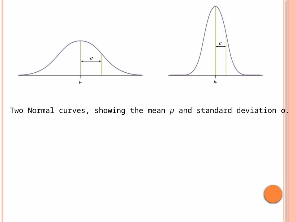
All Normal curves are symmetric, single-peaked, and bell-shaped

A specific Normal curve is described by giving its mean µ and standard deviation .σ

Two Normal curves, showing the mean µ and standard deviation σ.

Normal distributions are good descriptions for some distributions of

real data.

Normal distributions are good approximations of the results of many

kinds of chance outcomes.

Many statistical inference procedures are based on Normal distributions.

WARNING:There is NO such thing as a normal

curve in real life.

Things are only approximately normal.

WARNING2:You must use the adjective

approximately to describe normal distributions.

Because that’s what they are.

Don’t make me use my red pen on your work.

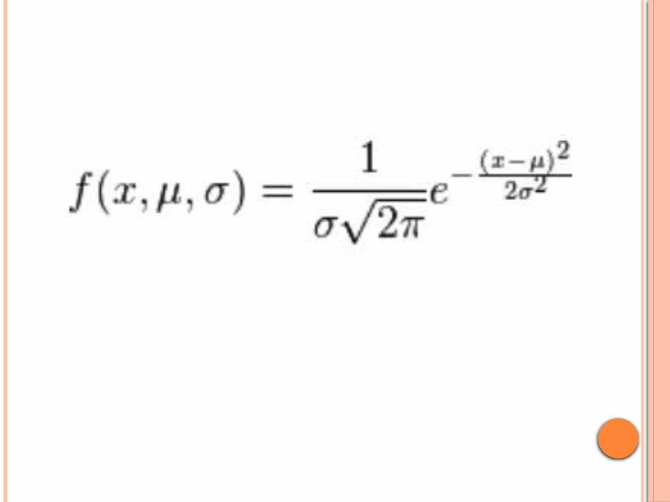
A Normal distribution is described by a Normal density curve. Any particular Normal distribution is completely specified by two numbers: its mean µ and standard deviation . σ

• The mean of a Normal distribution is the center of the symmetric Normal curve.

• The standard deviation is the distance from the center to the change-of-curvature points on either side. (Hello Calculus Magic)

• We abbreviate a Normal distribution with mean µ and standard deviation as σ N(µ,σ).

• I would like you to use approx as well.

Two Normal curves, showing the mean µ and standard deviation σ.

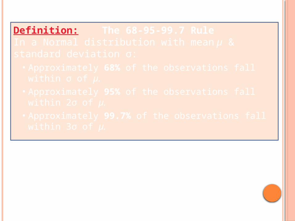
Definition: The 68-95-99.7 RuleIn a Normal distribution with mean µ & standard deviation :σ

• Approximately 68% of the observations fall within of σ µ.• Approximately 95% of the observations fall within 2 of σ µ.• Approximately 99.7% of the observations fall within 3 of σ µ.

After measuring many, many mothers, the authors of a biology paper published in 1903 argued

that the distribution of their heights was approx normally

distributed with a mean of 62.5 and a stdev of 2.4 inches.

The compression strength of concrete is approx normally

distributed with mean 3000 psi and stdev 500.

The speed of a car involved in a fatal car crash is approx normally

distributed with mean 51 mph and stdev 18 mph.

The heights of young American women are approx normally

distributed with mean 64.5 inches and stdev 2.5 inches.

www.whfreeman.com/tps4e

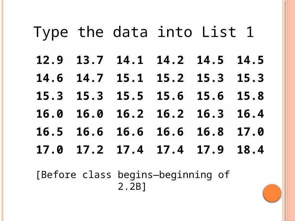
12.9 13.7 14.1 14.2 14.5 14.514.6 14.7 15.1 15.2 15.3 15.315.3 15.3 15.5 15.6 15.6 15.816.0 16.0 16.2 16.2 16.3 16.416.5 16.6 16.6 16.6 16.8 17.017.0 17.2 17.4 17.4 17.9 18.4

Type the data into List 1

[Before class begins—beginning of 2.2B]

Homework Comments:

• When comparing, use comparison language. • If you are comparing two people/things with z-score, make sure to use z-score in explanation• INTERPRET! (z-score)• Plot your data

2.2B INTRODUCTION TO NORMAL DISTRIBUTIONS

After this section, you should be able to…

PERFORM Normal distribution calculations using tables and/or technology

ASSESS Normality

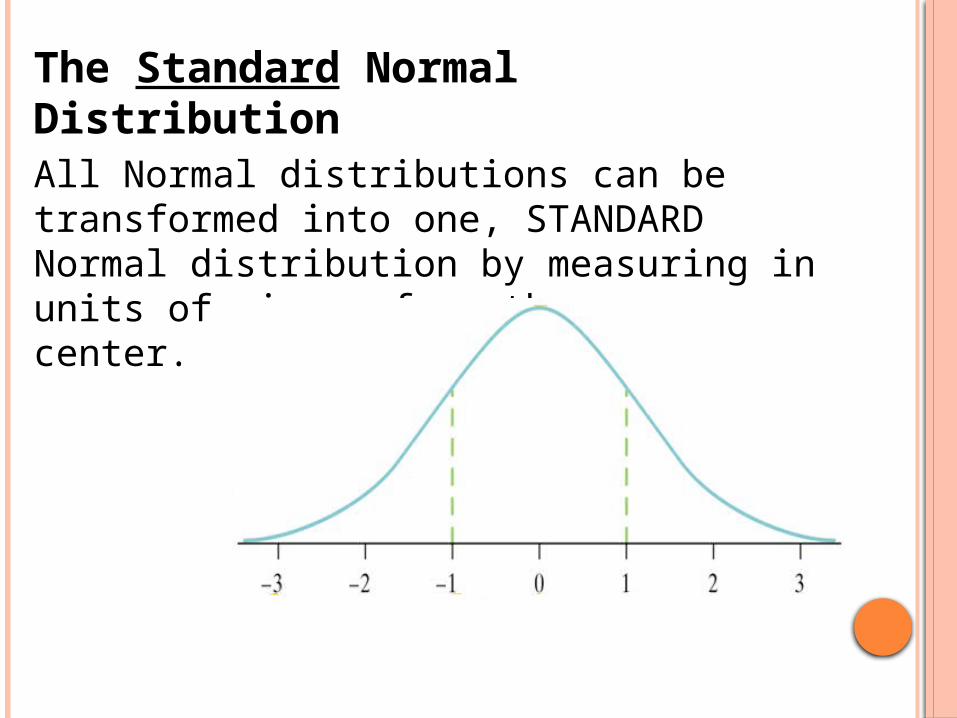
The Standard Normal DistributionAll Normal distributions can be transformed into one, STANDARD Normal distribution by measuring in units of size from the mean σ µ as center.

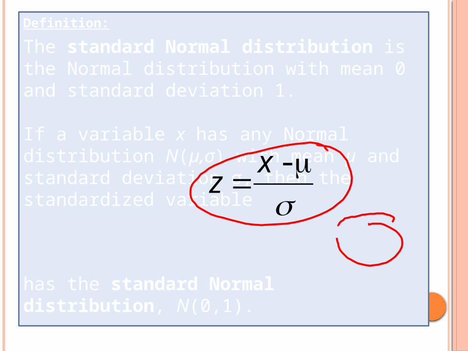
Definition:

The standard Normal distribution is the Normal distribution with mean 0 and standard deviation 1.

If a variable x has any Normal distribution N(µ,σ) with mean µ and standard deviation , then the σstandardized variable

has the standard Normal distribution, N(0,1).

z x -

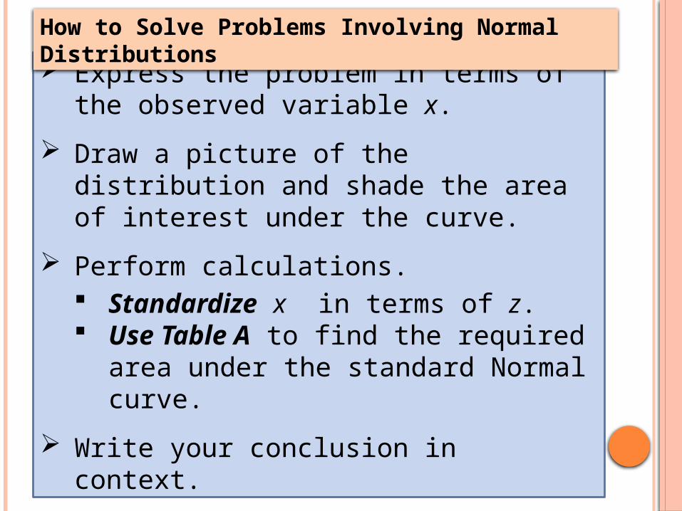
Express the problem in terms of the observed variable x.

Draw a picture of the distribution and shade the area of interest under the curve.

Perform calculations. Standardize x in terms of z. Use Table A to find the required area

under the standard Normal curve.

Write your conclusion in context.

How to Solve Problems Involving Normal Distributions

The heights of young American women are approx normally

distributed with mean 64.5 inches and stdev 2.5 inches.

The heights of young American women are approx normally

distributed with mean 64.5 inches and stdev 2.5 inches.

1. What % are taller than 68”?

The heights of young American women are approx normally

distributed with mean 64.5 inches and stdev 2.5 inches.

2. What % are shorter than 60”?

The heights of young American women are approx normally

distributed with mean 64.5 inches and stdev 2.5 inches.

3. What % are between 60”and 68”?

The heights of young American women are approx normally

distributed with mean 64.5 inches and stdev 2.5 inches.

4. How tall would a person in the top ten percent have to be?

Assessing Normality(I am going to say something like this, but you

don’t need to copy this down )

The Normal distributions provide good models for some distributions of real data. Many

statistical inference procedures are based on the assumption that the population is approximately Normally distributed. Consequently, we need a

strategy for assessing Normality.

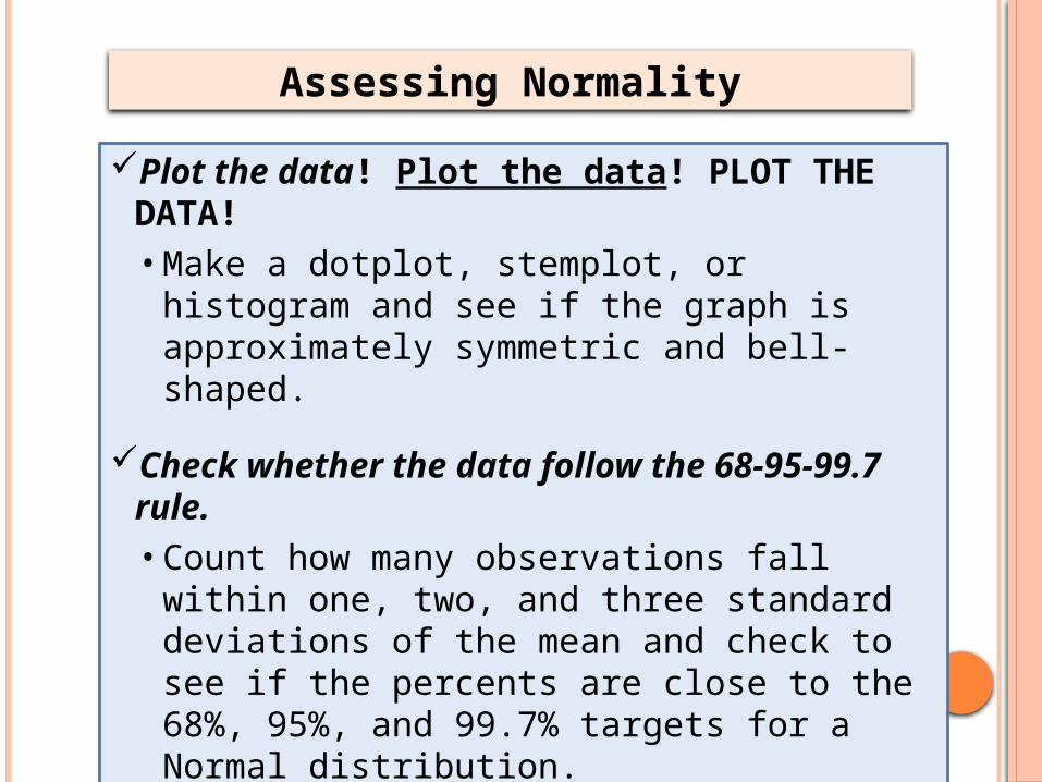
Plot the data! Plot the data! PLOT THE DATA!• Make a dotplot, stemplot, or histogram and see if

the graph is approximately symmetric and bell-shaped.

Check whether the data follow the 68-95-99.7 rule. • Count how many observations fall within one, two,

and three standard deviations of the mean and check to see if the percents are close to the 68%, 95%, and 99.7% targets for a Normal distribution.

Assessing Normality

12.9 13.7 14.1 14.2 14.5 14.514.6 14.7 15.1 15.2 15.3 15.315.3 15.3 15.5 15.6 15.6 15.816.0 16.0 16.2 16.2 16.3 16.416.5 16.6 16.6 16.6 16.8 17.017.0 17.2 17.4 17.4 17.9 18.4

 

Plot the data. (Do I need to say it thrice?)• Make a dotplot, stemplot, or histogram and see if

the graph is approximately symmetric and bell-shaped.

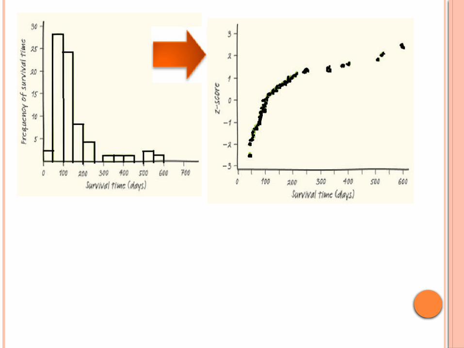
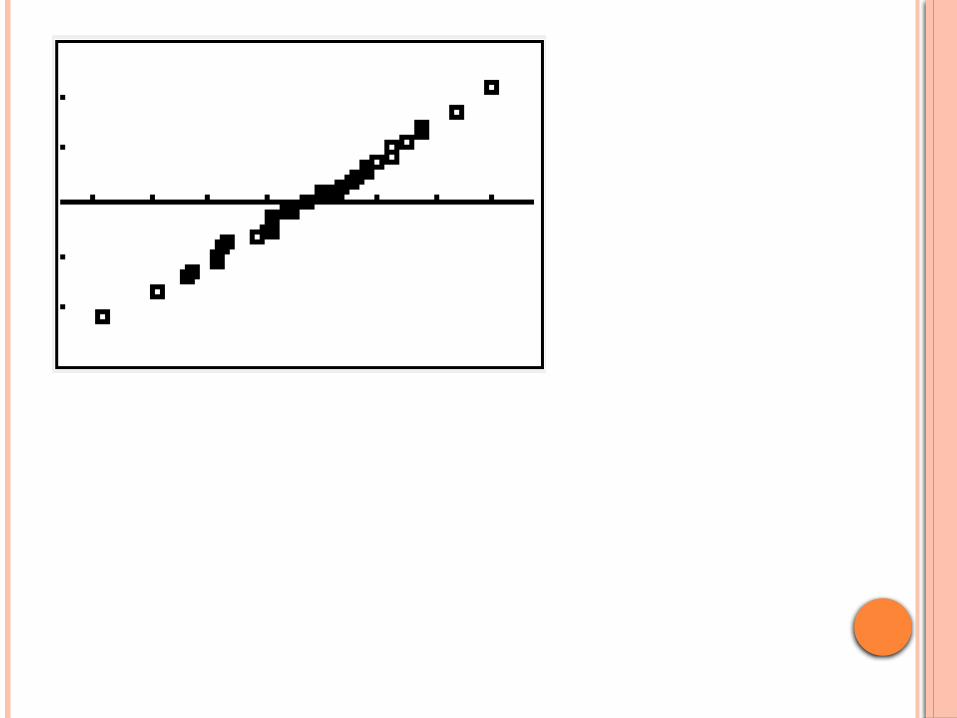
Use a Normal Probability Plot. • Sketch a Normal Probability Plot• Assess the NPP for approximate normality

Assessing Normality

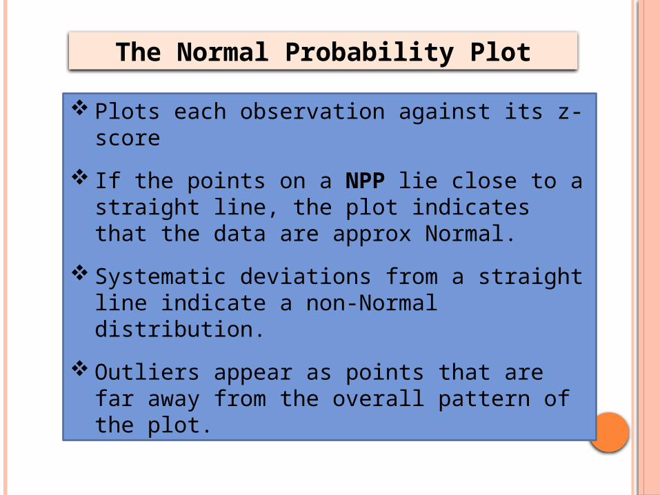
The Normal Probability Plot

Plots each observation against its z-score

If the points on a NPP lie close to a straight line, the plot indicates that the data are approx Normal.

Systematic deviations from a straight line indicate a non-Normal distribution.

Outliers appear as points that are far away from the overall pattern of the plot.

The heights of young American women are approx normally distributed with

mean 64.5 inches and stdev 2.5 inches.

1. % taller than 68”2. % shorter than 60”3. % between 60” and 68”