23/01/07 2ndversionforrussianmathsurveys · 23/01/07 2ndversionforrussianmathsurveys 3 nonlinear...

arX

iv:m

ath-

ph/0

6100

04v2

9 M

ar 2

007

23/01/07 2nd version for Russian Math Surveys 1

Ortho-normal quaternion frames, Lagrangian evolution equations and the

three-dimensional Euler equations1

J. D. Gibbon

Department of Mathematics, Imperial College London2, London SW7 2AZ, UK

Abstract

More than 160 years after their invention by Hamilton, quaternions are now widely used

in the aerospace and computer animation industries to track the orientation and paths of

moving objects undergoing three-axis rotations. It is shown here that they provide a natural

way of selecting an appropriate ortho-normal frame – designated the quaternion-frame – for

a particle in a Lagrangian flow, and of obtaining the equations for its dynamics. How these

ideas can be applied to the three-dimensional Euler fluid equations is then considered. This

work has some bearing on the issue of whether the Euler equations develop a singularity

in a finite time. Some of the literature on this topic is reviewed, which includes both the

Beale-Kato-Majda theorem and associated work on the direction of vorticity by Constantin,

Fefferman & Majda and Deng, Hou and Yu. It is then shown how the quaternion formulation

provides an alternative formulation in terms of the Hessian of the pressure.

This paper is dedicated to the memory of Victor Yudovich (1934-2006) with whom the author

discussed some of these ideas in their early stages.

Contents

1 General introduction 2

1.1 Historical remarks . . . . . . . . . . . . . . . . . . . . . . . . . . . . . . . . . . . . . . . . 2

1.2 Application to fluid dynamics . . . . . . . . . . . . . . . . . . . . . . . . . . . . . . . . . . 2

1.3 Blow-up in the three-dimensional Euler equations . . . . . . . . . . . . . . . . . . . . . . . 5

1.4 Definition & properties of quaternions . . . . . . . . . . . . . . . . . . . . . . . . . . . . . 6

2 Lagrangian evolution equations and an ortho-normal frame 8

3 Quaternions and the incompressible 3D Euler equations 11

4 The BKM Theorem & the direction of vorticity 13

4.1 The work of Constantin, Fefferman & Majda . . . . . . . . . . . . . . . . . . . . . . . . . 14

4.2 The work of Deng, Hou & Yu . . . . . . . . . . . . . . . . . . . . . . . . . . . . . . . . . . 16

4.3 The non-constancy of αp & χp: quaternions & the direction of vorticity . . . . . . . . . . 17

5 A final example: the equations of incompressible ideal MHD 18

6 Conclusion 19

1The material in this review is based on the contents of an invited lecture given at the meeting Mathematical

Hydrodynamics held at the Steklov Institute Moscow, in June 2006.2email address: [email protected]

http://arxiv.org/abs/math-ph/0610004v2


1 General introduction

1.1 Historical remarks

Everyone loves a good story : William Rowan Hamilton’s feverish excitement at the discovery

of his famous formula for quaternions on 16th October 1843 as a composition rule for orienting

his telescope; his inscription of this formula on Broome (Brougham) Bridge in Dublin; and then

his long and eventually unfruitful championing of the role of quaternions in mechanics, are all

elements of a story that has lost none of its appeal [1, 2]. Hamilton’s name is still revered today

for the audacity and depth of his ideas in modern mechanics and what we now call symplectic

geometry [3, 4, 5]. Indeed, evidence of his thinking is everywhere in both classical and quantum

mathematical physics and applied mathematics, yet in his own century his work on quater-

nions evoked criticism and even derision from many influential fellow scientists3. Ultimately

quaternions lost out to the tensor notation of Gibbs, which is the basis of the 3-vector notation

universally used today.

In essence, Hamilton’s multiplication rule for quaternions represents compositions of rota-

tions [6, 7, 8, 9, 10, 11]. This property has been ably exploited in modern inertial guidance

systems in the aerospace industry where computing the orientation and the paths of rapidly

moving rotating satellites and aircraft is essential. Kuipers’ book explains the details of how

calculations with quaternions in this field are performed in practice [12]. Just as importantly,

the computer graphics community also uses them to determine the orientation of tumbling ob-

jects in animations. In his valuable and eminently readable book, Andrew Hanson [2] says in

his introduction :

Although the advantages of the quaternion forms for the basic equations of attitude control –

clearly presented in Cayley [6], Hamilton [7, 8] and especially Tait [9] – had been noticed by

the aeronautics and astronautics community, the technology did not penetrate the computer

animation community until the land-mark Siggraph 1985 paper of Shoemake [13]. The

importance of Shoemake’s paper is that it took the concept of the orientation frame for

moving 3D objects and cameras, which require precise orientation specification, exposed

the deficiencies of the then-standard Euler-angle methods4, and introduced quaternions to

animators as a solution.

Hamilton’s 19th century critics were, of course, correct in their assertion that quaternions need 3-

vector algebra to manipulate them, yet the use the aero/astronautics and animation communities

have made of them are one more illustration of the universally acknowledged truth that while

new mathematical tools may not be of immediate use, and may appear to be too abstract or

overly elaborate, they may nevertheless turn out to have powerful applications undreamed of at

the time of their invention.

1.2 Application to fluid dynamics

The close association of quaternions with rigid body rotations [9, 10, 11] points to their use

in the incompressible Euler equations for an inviscid fluid as a natural language for describing

the alignment of vorticity with the eigenvectors of the strain rate that are responsible for its

3Kelvin was one such example: see [1].4A well-known deficiency of Euler-angle methods lies in the problems they suffer at the poles of the sphere

where the azimuthal angle is not defined.


nonlinear evolution. For a three-dimensional fluid velocity field u(x, t) with pressure p(x, t),

the incompressible Euler equations are [14, 15, 16, 17, 18]

Du

Dt= −∇p , (1.1)

where the material derivative is defined by

D

Dt=

∂

∂t+ u · ∇ . (1.2)

The motion is constrained by the incompressibility condition divu = 0. The crucial dynamics lies

in the evolution of the velocity gradient matrix ∇u = ui,j which comes from the differentiation

of (1.1)Dui,jDt

= −ui,kuk,j − Pij , (1.3)

where Pij is the Hessian matrix of the pressure

Pij =∂2p

∂xi∂xj. (1.4)

The incompressibility condition divu = 0 insists that Tr ui,j = 0 which, when applied to (1.3),

gives

Tr P = ∆p = −ui,kuk,i = 1

2ω2 − Tr (S2) . (1.5)

In (1.5) above, S is the strain matrix whose elements are defined by

Sij = 1

2(ui,j + uj,i) . (1.6)

This is a symmetric matrix the alignment of whose eigenvectors ei is fundamental to the dynam-

ics of the Euler equations. For instance, vortex tubes and sheets (Burgers’ vortices and shear

layers) always have one eigenvector aligned with the vorticity vector ω [18].

This review cannot hope to deal with every aspect of the three-dimensional Euler equations,

particularly the vast literature on weak and distributional solutions; the reader is urged to read

the book by Majda & Bertozzi [15] to study these aspects of the problem. Here we concentrate

on one particular aspect, which is the role played by quaternions in providing a natural language

for extracting geometric information from the evolution of ui,j. Because they are particularly

effective in computing the orientation of rotating objects moving in three-dimensional paths they

might be useful in understanding how general Lagrangian flows behave, particularly in finding

the evolution of the ortho-normal frame of particles moving in such a flow. These particles could

be of the passive tracer type transported by a background flow or they could be Lagrangian fluid

parcels. Recent experiments in turbulent flows can now detect the trajectories of tracer particles

at high Reynolds numbers [19, 20, 21, 22, 23, 24, 25, 26, 27, 28] : see Figure 1 in [19]. For any

system involving a path represented as a three-dimensional space-curve, the usual practice is

to consider the Frenet-frame of a trajectory constituted by the unit tangent vector, the normal

and the bi-normal [2, 28]. In navigational language, this represents the corkscrew-like pitch,

yaw and roll of the motion. While the Frenet-frame describes the path, it ignores the dynamics

that generates the motion. Attempts have been made in this direction using the eigenvectors

ei of S but ran into difficulties because the equations of motion for ei are unknown [29]. In §2

another ortho-normal frame is introduced that is associated with the motion of each Lagrangian


particle. It is designated the quaternion-frame : this frame may be envisioned as moving with

the Lagrangian particles, but its evolution derives from the Eulerian equations of motion. The

advantage of this approach lies in the fact that the Lagrangian dynamics of the quaternion-frame

can be connected to the fluid motion through the pressure Hessian P defined in (1.4).

Let us now consider a general picture of a Lagrangian flow system of equations. Supposew is

a contravariant vector quantity attached to a particle following a flow along characteristic paths

dx/dt = u(x, t) of a velocity field u. Let us consider the abstract Lagrangian flow equation

Dw

Dt= a(x, t) ,

D

Dt=

∂

∂t+ u · ∇ , (1.7)

where the material derivative has its standard definition, and that, in turn, a satisfies the

Lagrangian equationD2w

Dt2=

Da

Dt= b(x, t) . (1.8)

So far, these are just kinematic rates of change following the characteristics of the velocity

generating the path x(t) determined from dx/dt = u(x, t). Examples of systems that (1.7)

might represent are :

1. If w represents the vorticity ω = curlu of the incompressible Euler fluid equations then

a = ω · ∇u and divu = 0. With rotation w would be w ≡ ω = ρ−10 (ω + 2Ω).

2. For the barotropic compressible Euler fluid equations (where the pressure p = p(ρ) is

density dependent only) then w ≡ ωρ = ρ−1ω, in which case a = ωρ · ∇u and divu = 0.

3. w could also represent a small vectorial line element δℓ that is mixed and stretched by a

background flow u, in which case a = δℓ · ∇u. For example, following Moffatt’s analogy

with between the magnetic field B in ideal incompressible MHD and vorticity [30], if w is

chosen such that w ≡ B, then a = B · ∇u with divB = 0. In a more generalized form

it could also represent the Elsasser variables w± = u ±B, in which case a± = w± · ∇u

with two material derivatives.

4. The semi-geostrophic (SG) model used in atmospheric physics can also be cast in the

form of (1.7) ; for instance one could choose w = x, a = u and b is computed from the

SG-model through the semi-geostrophic and a-geostrophic contributions [31, 32, 33].

5. For a passive tracer particle with velocity w in a fluid transported by a background velocity

field u, the particle’s acceleration would be a (see [34, 16]).

In cases (1–3) above if w satisfies the standard Eulerian form

Dw

Dt= w · ∇u , (1.9)

then to find b it follows from Ertel’s Theorem that [35]

D(w · ∇µ)

Dt= w · ∇

(

Dµ

Dt

)

, (1.10)

which means that the operators D/Dt and w ·∇ commute for any differentiable function µ(x, t).

Choosing µ = u as in [36], and identifying the flow acceleration as Q(x, t) such that Du/Dt =

Q(x, t), we haveD2w

Dt2= w · ∇

(

Du

Dt

)

= w · ∇Q . (1.11)


In each of the cases (1-3) above Q is readily identifiable and thus we have b

Da

Dt= w · ∇Q =: b(x, t) , (1.12)

thereby completing the quartet of vectors (u, w, a, b). In §2 it will be shown that knowledge

of the quartet of vectors (u, w, a, b) determines the quaternion-frame, which is a completely

natural ortho-normal frame for the Lagrangian dynamics. Modulo a rotation around w, the

quaternion-frame turns out to be the Frenet-frame attached to lines of constant w. Although

usually credited to Ertel [35], the result in (1.10), which involves the cancellation of nonlinear

terms of O(|w||∇u|2), actually goes much further back in the literature than this; see [36, 37,

38, 39, 40]. While Ertel’s Theorem above enables us to find a b as in cases (1-3), b must be

determined by other means in case (4).

1.3 Blow-up in the three-dimensional Euler equations

The general picture of Lagrangian evolution and the associated quaternion frame is given in §2.

Thereafter this paper will focus on the three-dimensional incompressible Euler equations (1.1)

(see §3) and the global existence of solutions (see §4).

Many generations of mathematicians could testify to the deceptive simplicity of the Euler

equations. The work of the late Victor Yudovich [41], who proved the existence and uniqueness

of weak solutions of the two-dimensional Euler equations with ω0 ∈ L∞ on unbounded domains,

will be remembered as a mile-stone in Euler dynamics. In the three-dimensional case, while many

special solutions are known in terms of simple functions [16, 17, 18], and powerful results have

been found on weak and distributional solutions (see Majda & Bertozzi [15]) yet the fundamental

problem of whether solutions exist for arbitrarily long times or become singular in a finite time

still remains open. In physical terms, singular behaviour could potentially occur if a vortex is

resolvable only by length scales decreasing to zero in a finite time. While a review of certain

aspects of the three-dimensional Euler singularity problem will form part of the later sections of

this review, the regularity problem for the Navier-Stokes equations will not be considered; the

interested reader should consult [42, 43, 44].

In the first demonstrable case of Euler blow-up, Stuart [45, 46, 47] considered solutions of

the three-dimensional Euler equations that had linear dependence in two variables x and z;

the resulting differential equations in the remaining independent variables y and t displayed

finite time singular behaviour. Stuart then showed how the method of characteristics leads

to the construction of a complete class of singular solutions [45]. This type of singularity has

infinite energy because the solution is linearly stretched in the both the x and z directions.

In a similar fashion, Gibbon, Fokas & Doering [48] considered another class of infinite energy

solutions whose third component of velocity is linear in z so that the velocity field takes the form

u = u1(x, y, t), u2(x, y, t), zγ(x, y, t). These generalize the Burgers’ vortex [18] and represent

tube and ring-like structures depending on the sign of γ(x, y, t). Strong numerical evidence of

singular behaviour on a periodic x − y cross-section found by Ohkitani and Gibbon [49] was

confirmed by an analytical proof of blow-up by Constantin [50]. Subsequently Gibbon, Moore

and Stuart [51] found two explicit singular solutions using the methods outlined in [45].

The Beale-Kato-Majda (BKM) theorem [52] has been the main cornerstone of the analysis

of potential finite energy Euler singularities : one version of this theorem is that ‖ω‖∞ must


satisfy (see §4 for a more precise statement)

∫ T

0‖ω‖∞ dτ < ∞ , (1.13)

for a global solution to exist up to time T . The most important feature of (1.13) is that it is

single, simple criterion which is easily monitored. Several refinements of the BKM-Theorem exist

in addition to those by Ponce [53], who replaced ‖ω‖∞ by ‖S‖∞, and the BMO-version proved

by Kozono and Taniuchi [54]. In particular, these take account of the direction in which vorticity

grows. The work of Constantin [55], and Constantin, Fefferman & Majda [56], reviewed in §4.1,

deserves specific mention. They were the first to make a precise mathematical formulation of

how the misalignment of vortex lines might lead to, or prevent, a singularity. §4.2 is devoted

to a review of the work of Deng, Hou & Yu [57, 58] who have established different criteria on

vortex lines. In §4.3, quaternions are considered as an alternative way of looking at the direction

of vorticity [59], which provides us with a different direction of vorticity theorem based on the

Hessian matrix of the pressure (1.4). Further discussion and references are left to §4.

1.4 Definition & properties of quaternions

In terms of any scalar p and any 3-vector q, the quaternion q = [p, q] is defined as (Gothic fonts

denote quaternions)

q = [p, q] = pI −

3∑

i=1

qiσi , (1.14)

where σ1, σ2, σ3 are the three Pauli spin-matrices defined by

σ1 =

(

0 i

i 0

)

, σ2 =

(

0 1

−1 0

)

, σ3 =

(

i 0

0 −i

)

, (1.15)

and which obey the relations σiσj = −δijI − ǫijkσk . I is the 2× 2 unit matrix. These relations

then give a non-commutative multiplication rule

q1 ⊛ q2 = [p1p2 − q1 · q2, p1q2 + p2q1 + q1 × q2] . (1.16)

It can easily be demonstrated that quaternions are associative. One of the main properties of

quaternions not shared by 3-vectors is the fact that they have an inverse; the inverse of q is

q∗ = [p, −q] which means that q ⊛ q∗ = [p2 + q2, 0] = (p2 + q2)[1, 0]; of course, [1, 0] really

denotes a scalar so if p2 + q2 = 1, q is a unit quaternion q.

A quaternion of the type w = [0, w] is called a pure quaternion, with the product between

two of them expressed as

w1 ⊛w2 = [0, w1]⊛ [0, w2] = [−w1 ·w2, w1 ×w2] . (1.17)

In fact there is a quaternionic version of the gradient operator ∇ = [0, ∇] which, when acting

upon a pure quaternion u = [0, u], gives

∇⊛ u = [−divu, curlu] . (1.18)

If the field u is divergence-free, as for an incompressible fluid, then

∇⊛ u = [0, ω] . (1.19)


This pure quaternion incorporating the vorticity will be used freely in future sections.

It has been mentioned already in Section 1.1 that quaternions are used in the aerospace

and computer animation industries to avoid difficulties with Euler angles. Here the relation is

briefly sketched between quaternions and one of the many ways that have been used to describe

rotating bodies in the rich and long-standing literature of classical mechanics – for more see

[62]. Whittaker [10] shows how quaternions and the Cayley-Klein parameters [11] are intimately

related and gives explicit formulae relating these parameters to the Euler angles. Let q = [p, q]

be a unit quaternion with inverse q∗ = [p, −q] where p2+q2 = 1. For a pure quaternion r = [0, r]

there exists a transformation from r → r′ = [0, r′]

r′ = q⊛ r⊛ q

∗ . (1.20)

This associative product can explicitly be written as

r′ = q⊛ r⊛ q

∗ = [0, (p2 − q2)r + 2p(q × r) + 2q(r · q)] . (1.21)

Choosing p = ± cos 1

2θ and q = ± n sin 1

2θ, where n is the unit normal to r, we find that

r′ = q⊛ r⊛ q

∗ = [0, r cos θ + (n× r) sin θ] ≡ O(θ, n)r , (1.22)

Equation (1.22) is the Euler-Rodrigues formula for the rotation O(θ, n) by an angle θ of the

vector r about its unit normal n ; θ and n are called the Euler parameters. With the choice of

p and q above q is given by

q = ±[cos 1

2θ, n sin 1

2θ] . (1.23)

The elements of the unit quaternion q are the Cayley-Klein parameters which are related to the

Euler angles and which form a representation of the Lie group SU(2). All terms in the (1.21)

are quadratic in p and q, and thus possess the well-known ± equivalence which is an expression

of the fact that SU(2) covers SO(3) twice.

To investigate the map (1.20) when p is time-dependent, the Euler-Rodrigues formula in

(1.22) can be written as

r′(t) = p⊛ r⊛ p

∗ ⇒ r = p∗ ⊛ r

′(t)⊛ p . (1.24)

Thus r′ has a time derivative given by

r′(t) = ˙p⊛ (p∗ ⊛ r

′ ⊛ p)⊛ p∗ + p⊛ (p∗ ⊛ r

′ ⊛ p)⊛ ˙p∗

= ˙p⊛ p∗ ⊛ r

′ + r′ ⊛ p⊛ ˙p∗

= (˙p⊛ p∗)⊛ r

′ + r′ ⊛ ( ˙p⊛ p

∗)∗

= (˙p⊛ p∗)⊛ r

′ − (( ˙p ⊛ p∗)⊛ r

′)∗ , (1.25)

having used the fact on the last line that because r′ is a pure quaternion, r′∗ = −r′. Because

p = [p, q] is of unit length, and thus pp+qq = 0, this means that ˙p⊛ p∗ is also a pure quaternion

˙p⊛ p∗ = [0, 1

2Ω0(t)] . (1.26)

The 3-vector entry in (1.26) defines the angular frequency Ω0(t) as Ω0 = 2(−pq + qp− q × q)

thereby giving the well-known formula for the rotation of a rigid body

r′ = Ω0 × r′ . (1.27)


For a Lagrangian particle, the equivalent of Ω0 is the Darboux vector Da in Theorem 1 of §2.

This Theorem is the main result of this paper and is the equivalent of (1.27) for a Lagrangian

particle undergoing rotation in flight.

Finally, it can easily be seen that Hamilton’s relation in terms of hyper-complex numbers

i2 = j2 = k2 = ijk = −1 will generate the rule in (1.16) if q is written as a 4-vector q =

p + iq1 + jq2 + kq3. Sudbery’s paper is still the best source for a study of the functional

properties of quaternions [60]; he discusses how various results familiar for functions over a

complex field, such as the Cauchy-Riemann equations, Cauchy’s Theorem and integral formula,

together with the Laurent expansion (but not conformal mappings) have their parallels for

quaternionic functions. More recent work on further analytical properties can be found in [61].

2 Lagrangian evolution equations and an ortho-normal frame

This section sets up the mathematical foundation concerning the association of quaternion

frames and can be found in the paper by Gibbon and Holm [62]. Let us repeat the Lagrangian

evolution equations for a vector field w satisfying (1.7) and (1.8)

Dw

Dt= a(x, t) ,

Da

Dt= b(x, t) . (2.1)

•(x1, t1)

w

χa

w × χa •(x2, t2) w

❳❳❳③

w × χa

χa

tracer particle trajectory

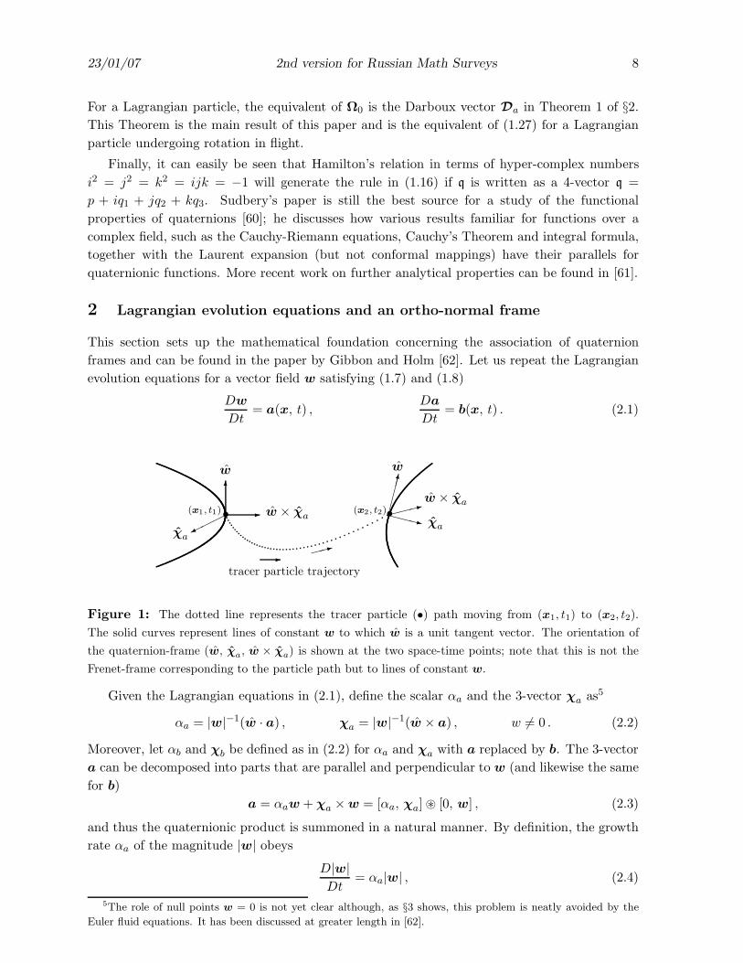
Figure 1: The dotted line represents the tracer particle (•) path moving from (x1, t1) to (x2, t2).

The solid curves represent lines of constant w to which w is a unit tangent vector. The orientation of

the quaternion-frame (w, χa, w × χ

a) is shown at the two space-time points; note that this is not the

Frenet-frame corresponding to the particle path but to lines of constant w.

Given the Lagrangian equations in (2.1), define the scalar αa and the 3-vector χa as5

αa = |w|−1(w · a) , χa = |w|−1(w × a) , w 6= 0 . (2.2)

Moreover, let αb and χb be defined as in (2.2) for αa and χa with a replaced by b. The 3-vector

a can be decomposed into parts that are parallel and perpendicular to w (and likewise the same

for b)

a = αaw + χa ×w = [αa, χa]⊛ [0, w] , (2.3)

and thus the quaternionic product is summoned in a natural manner. By definition, the growth

rate αa of the magnitude |w| obeys

D|w|

Dt= αa|w| , (2.4)

5The role of null points w = 0 is not yet clear although, as §3 shows, this problem is neatly avoided by the

Euler fluid equations. It has been discussed at greater length in [62].


while the unit tangent vector w = ww−1 satisfies

Dw

Dt= χa × w . (2.5)

Now identify the quaternions6

qa = [αa, χa] , qb = [αb, χb] , (2.6)

and let w = [0, w] be the pure quaternion satisfying the Lagrangian evolution equation (2.1) with

qa defined in (2.6). Then the first equation in (2.1) can automatically be re-written equivalently

in the quaternion form

Dw

Dt= [0, a] = [0, αaw + χa ×w] = qa ⊛w . (2.7)

Moreover, if a is differentiable in the Lagrangian sense as in (2.1) then it is clear that a similar

decomposition for b as that for a in (2.3) gives

D2w

Dt2= [0, b] = [0, αbw + χb ×w] = qb ⊛w . (2.8)

Using the associativity property, compatibility of (2.8) and (2.7) implies that (|w| 6= 0)

(

Dqa

Dt+ qa ⊛ qa − qb

)

⊛w = 0 , (2.9)

which establishes a Riccati relation between qa and qb

Dqa

Dt+ qa ⊛ qa = qb . (2.10)

This relation is closely allied to the ortho-normal quaternion-frame7 (w, χa, w × χa) whose

equations of motion are given as follows :

Theorem 1 [62] The ortho-normal quaternion-frame (w, χa, w×χa) ∈ SO(3) has Lagrangian

time derivatives expressed as

Dw

Dt= Dab × w , (2.11)

D(w × χa)

Dt= Dab × (w × χa) , (2.12)

Dχa

Dt= Dab × χa , (2.13)

where the Darboux angular velocity vector Dab is defined as

Dab = χa +cbχa

w , cb = w · (χa × χb) . (2.14)

Remark: The analogy with the formula for a rigid body is obvious when compared to (1.27).

but the Darboux angular velocity vector Dab is itself a function of χ , w and other variables

and sits in a two-dimensional plane. In turn this is driven by cb = w · (χa × χb) for which b

6Dropping the a , b labels and normalizing, the Cayley-Klein parameters are q = [α, χ](α2 + χ2)−1/2.7According to Hanson [2] the the quaternion-frame is similar to the Bishop-frame in computer graphics.


must be known. Given this it may then possible to numerically solve equations (2.11) – (2.14)

for the particle paths.

Proof : To find an expression for the Lagrangian time derivatives of the components of the

frame (w, χa, w × χa) requires the derivative of χa. To find this it is necessary to use the fact

that the 3-vector b can be expressed in this ortho-normal frame as the linear combination

w−1b = αb w + cbχa + db(w × χa) . (2.15)

where cb is defined in (2.14) and db = − (χa ·χb). The 3-vector product χb = w−1(w× b) yields

χb = cb(w × χa)− dbχa . (2.16)

To find the Lagrangian time derivative of χa, we use the 3-vector part of the equation for the

quaternion qa = [αa, χa] in Theorem 1

Dχa

Dt= −2αaχa + χb , ⇒

Dχa

Dt= −2αaχa − db , (2.17)

where χa = |χa|. Using (2.16) and (2.17) there follows

Dχa

Dt= cbχ

−1a (w × χa) ,

D(w × χa)

Dt= χa w − cbχ

−1a χa , (2.18)

which gives equations (2.11)-(2.14).

How to find the rate of change of acceleration represented by the b-vector is an important

question regarding computing the paths of passive tracer particles where b is not known through

Ertel’s Theorem. The result that follows describes the evolution of qb in terms of three arbitrary

scalars.

Theorem 2 [62] The Lagrangian time derivative of qb can be expressed as

Dqb

Dt= qa ⊛ qb + λ1qb + λ2qa + λ3I , (2.19)

where the λi(x, t) are arbitrary scalars (I = [1, 0]).

Proof : To establish (2.19), we differentiate the orthogonality relation χb · w = 0 and use the

Lagrangian derivative of w

Dχb

Dt= χa × χb + s0 , where s0 = µχa + λχb . (2.20)

s0 lies in the plane perpendicular to w in which χa and χb also lie and µ = µ(x, t) and λ = λ(x, t)

are arbitrary scalars. Explicitly differentiating χb = w−1(w × b) gives

w−1w (χa · b) + s0 = −αaχb − αbχa + w−1w (χa · b) +w−1

(

w ×Db

Dt

)

, (2.21)

which can easily be manipulated into

w ×

Db

Dt− αb a− αa b

= w s0 . (2.22)

This means thatDb

Dt= αba+ αab+ s0 ×w + εw , (2.23)


where ε = ε(x, t) is a third unknown scalar in addition to µ and λ in (2.20). Thus the Lagrangian

derivative of αb = w−1(w · b) is

Dαb

Dt= ααb +χa · χb + ε . (2.24)

Lagrangian differential relations have now been found for χb and αb, but at the price of intro-

ducing the triplet of unknown coefficients µ, λ, and ε which are re-defined as

λ = αa + λ1 , µ = αb + λ2 , ε = −2χa · χb + λ2αa + λ1αb + λ3 . (2.25)

The new triplet has been subsumed into (2.19). Then (2.20) and (2.24) can be written in the

quaternion form (2.19).

3 Quaternions and the incompressible 3D Euler equations

The results of the previous section on Lagrangian flows are immediately applicable to the in-

compressible Euler equations, but to present them in this manner is actually to do so in the

chronologically reverse order in which they were first developed. Looking ahead in this section,

the variables α and χ in (3.4) for the Euler equations, and the two coupled differential equations

that they satisfy (3.10), were first written down almost ten years ago in [63, 64] without the

help of quaternions. It was then discovered in [65] that these equations could be combined to

form a quaternionic Riccati equation. Finally, the more recent paper [59], in combination with

[62], put all these results in the form expounded in this present paper. Because data for the

three-dimensional Euler equations gets very rough very quickly it should be understood that all

our manipulations are formal.

In §2 it was shown that a knowledge of the quartet of vectors (u, w, a, b) is necessary to be

able to use the results of Theorem 1. With w ≡ ω and ω = curlu the vortex stretching vector

is a = ω · ∇u. Thus the w- and u-fields are not independent in this case. Within a = ω · ∇u,

the dot-product of ω sees only the symmetric part of the velocity gradient matrix ∇u, which

is the strain matrix Sij = 1

2(ui,j + uj,i) defined in (1.6). With a = ω · ∇u = Sω, the triad of

vectors is

(u, w, a) ≡ (u, ω, Sω) . (3.1)

To find the b-field, Ertel’s Theorem of §1.2 comes to the rescue. The Du/Dt within the right

hand side of (1.1) (with w = ω) obeys Euler’s equation Du/Dt = −∇p, so we have

b = ω · ∇

(

Du

Dt

)

= −Pω , (3.2)

where P is the Hessian of the pressure defined in (1.4). The quartet of vectors necessary to

make Theorem 1 work is now in place

(u, w, a, b) ≡ (u, ω, Sω, −Pω) . (3.3)

The table below discusses three quartets (u, w, a, b) for the Euler fluid equations :

u w a b Material Deriv

Euler x u −∇p (1.2)

Euler u −∇p ? (1.2)

Euler ω Sω −Pω (1.2)


Table 1 : The entries above are three of the possibilities for finding a b-field given the triplet (u, w, a).

The third line is the result (3.3) while b is unknown for the second line.

Using the definitions in §2 the scalar α and the 3-vector χ are defined as

α = ω · Sω , χ = ω × Sω , (3.4)

together with the definitions for αp and χp

αp = ω · P ω , χp = ω × P ω . (3.5)

α in (3.4) is now identified as the same as that in Constantin [55] who has expressed it as an

explicit Biot-Savart formula8. a = Sω can be decomposed into parts that are parallel and

perpendicular to ω

Sω = αω +χ× ω = [α, χ]⊛ [0, ω] . (3.6)

By definition, the growth rate α of the scalar magnitude |ω| and the unit tangent vector ω obey

D|ω|

Dt= α|ω| ,

Dω

Dt= χ× ω , (3.7)

which show that α drives the growth or collapse of vorticity and χ determines the rate of swing

of ω around Sω. Now identify the quaternions

q = [α, χ] , qp = [αp, χp] . (3.8)

The equivalent of the Riccati equation (2.10) is9

Dq

Dt+ q⊛ q+ qp = 0 , (3.9)

which, when written explicitly in terms of α–χ, becomes

Dα

Dt+ α2 − χ2 + αp = 0 .

Dχ

Dt+ 2αχ + χp = 0 . (3.10)

In Theorem 1 we need to use b = −Pω to calculate the path of the ortho-normal quaternion-

frame (ω, χ, ω × χ). Specifically we must solve

Dω

Dt= D × ω , (3.11)

D(ω × χ)

Dt= D × (ω × χ) , (3.12)

Dχ

Dt= D × χ , (3.13)

where the Darboux angular velocity vector D is defined as

D = χ+cpχω , cp = −ω · (χ×χp) , (3.14)

The pressure Hessian contributes to the angular velocity D through the scalar coefficient cp.

To compute the fluid particle paths one would need data on the pressure Hessian P as well as

8Everywhere in [55, 56, 66, 67] the unit vector of vorticity is designated as ξ whereas here we use ω.9In principle (3.9) can be linearized to a zero-eigenvalue Schrodinger equation in quaternion form with qp as

the potential, although it is not clear how to proceed from that point.


the vorticity ω and the strain matrix S. It is here where the fundamental difference between

the Euler equations and a passive problem is made explicit. For the Euler equations the b-field

containing P is not independent of w ≡ ω but is connected subtly and non-locally through the

elliptic equation for the pressure (1.5) which we repeat here

− Tr P = Tr(S2)− 1

2ω2 . (3.15)

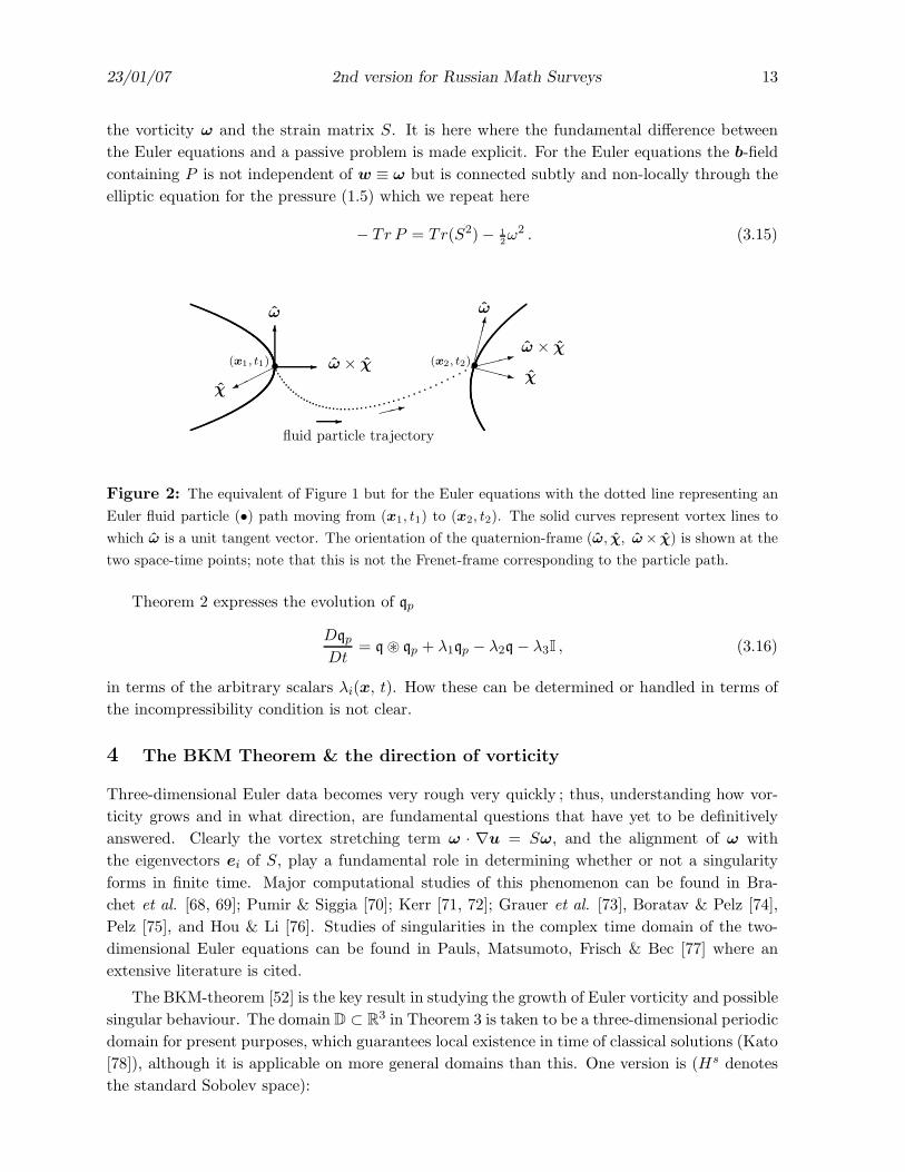
•(x1, t1)

ω

χ

ω × χ •(x2, t2) ω

❳❳❳③

ω × χ

χ

fluid particle trajectory

Figure 2: The equivalent of Figure 1 but for the Euler equations with the dotted line representing an

Euler fluid particle (•) path moving from (x1, t1) to (x2, t2). The solid curves represent vortex lines to

which ω is a unit tangent vector. The orientation of the quaternion-frame (ω, χ, ω× χ) is shown at the

two space-time points; note that this is not the Frenet-frame corresponding to the particle path.

Theorem 2 expresses the evolution of qp

Dqp

Dt= q⊛ qp + λ1qp − λ2q− λ3I , (3.16)

in terms of the arbitrary scalars λi(x, t). How these can be determined or handled in terms of

the incompressibility condition is not clear.

4 The BKM Theorem & the direction of vorticity

Three-dimensional Euler data becomes very rough very quickly ; thus, understanding how vor-

ticity grows and in what direction, are fundamental questions that have yet to be definitively

answered. Clearly the vortex stretching term ω · ∇u = Sω, and the alignment of ω with

the eigenvectors ei of S, play a fundamental role in determining whether or not a singularity

forms in finite time. Major computational studies of this phenomenon can be found in Bra-

chet et al. [68, 69]; Pumir & Siggia [70]; Kerr [71, 72]; Grauer et al. [73], Boratav & Pelz [74],

Pelz [75], and Hou & Li [76]. Studies of singularities in the complex time domain of the two-

dimensional Euler equations can be found in Pauls, Matsumoto, Frisch & Bec [77] where an

extensive literature is cited.

The BKM-theorem [52] is the key result in studying the growth of Euler vorticity and possible

singular behaviour. The domain D ⊂ R3 in Theorem 3 is taken to be a three-dimensional periodic

domain for present purposes, which guarantees local existence in time of classical solutions (Kato

[78]), although it is applicable on more general domains than this. One version is (Hs denotes

the standard Sobolev space):


Theorem 3 (Beale, Kato and Majda [52]) : On the domain D = [0, L]3per there exists a global

solution of the Euler equations, u ∈ C([0, ∞];Hs) ∩ C1([0, ∞];Hs−1) for s ≥ 3 if, for every

T > 0∫ T

0‖ω‖L∞(D) dτ < ∞ . (4.1)

The result can be stated the opposite way which is that no singularity can form at T without∫ T0 ‖ω‖L∞(D) dτ = ∞. Theorem 3 has direct computational consequences. In a hypothetical

computational experiment if one finds vorticity growth ‖ω‖L∞(D) ∼ (T − t)−γ for some γ > 0,

then the theorem says that γ must satisfy γ ≥ 1 for the observed singular behaviour to be real

and not an artefact of the numerical computations. The reason is that if γ is found to lie in

the range 0 < γ < 1 then ‖ω‖L∞(D) blows up whereas its time integral does not, thus violating

the theorem. Of the many numerical calculations performed on Euler that by Kerr [71, 72],

using anti-parallel vortex tubes as initial data, was the first to see γ pass the threshold with

a critical value of γ = 1, followed by Grauer et al. [73], Boratav & Pelz [74] and Pelz [75].

Recent numerical calculations by Hou & Li [76], however, have contradicted the existence of a

singularity: see [79] for a response and a discussion of the issues. To fully settle this question will

require more refined computations in tandem with analysis to understand the role played by the

direction of vorticity growth. As indicated in §1, the work of Constantin, Fefferman & Majda

[56] (see also Constantin [55]) was the first to make a precise mathematical formulation of how

smooth the direction of vortex lines have to be that might lead to, or prevent, a singularity. §4.1

is devoted to a short review of this work. Further papers by Cordoba & Fefferman [80], Deng,

Hou & Yu [57, 58] and Chae [66, 67] are variations on this theme. This approach, pioneered in

[56], lays the mathematical foundation for the next generation of computational experiments,

after the manner of Kerr [71, 72, 79] and Hou & Li [76], to check whether a singularity develops.

§4.2 is devoted to a description of the results in the papers by Deng, Hou & Yu [57, 58] who

have established different criteria on vortex lines. §4.3 is devoted to an alternative direction of

vorticity theorem proved in [59] based on the quaternion formulation of this paper.

References and a more global perspective on the Euler equations can be found in the book

by Majda and Bertozzi [15]. Shnirelman [81] has constructed very weak solutions which have

some realistic features but whose kinetic energy monotonically decreases in time and which

are everywhere discontinuous and unbounded and for its dynamics in the more exotic function

spaces see the papers by Tadmor [82] and Chae [83, 84, 85].

4.1 The work of Constantin, Fefferman & Majda

The obvious question regarding the BKM-criterion is whether the L∞-norm can be weakened

to Lp for 1 ≤ p ≤ ∞. This question was addressed by Constantin [55] who placed further

assumptions on the local nature of the vorticity and velocity fields. Consider the velocity field

U1(t) := supx

|u(x, t)|, (4.2)

and the L1loc-norm of ω defined by

‖ω‖1, loc = L−3 supx

∫

|y|≤L|ω(x+ y)|d3y , (4.3)


where L is some outer length scale in the Euler flow which could be taken to be unity. Now

assume that the unit vector of vorticity is Lipschitz

|ω(x, t)− ω(y, t)| ≤|x− y|

ρ0(t)(4.4)

for |x− y| ≤ L and for some length ρ0(t). Then the following result is stated in Constantin [55]

and re-stated and proved in Constantin, Fefferman & Majda [56]:

Theorem 4 (Constantin [55]; Constantin, Fefferman & Majda [56]) : Assume that the initial

vorticity ω0 is smooth and compactly supported and assume that a solution of the Euler equations

satisfies∫ T

0‖ω(· , s)‖1, loc

(

L

ρ0(s)

)3

ds < ∞ ,

∫ T

0

U(s)

ρ0(s)ds < ∞ . (4.5)

Then

sup0≤t≤T

‖ω(· , t)‖∞‖ω(· , t)‖1, loc

< ∞ . (4.6)

Clearly, if U1 = ‖u‖∞ < ∞ and ‖ω(· , t)‖1, loc < ∞ on [0, T ] and ρ0 is bounded away from zero

then the BKM theorem says that no singularities can arise. The Lipschitz condition (4.4) can

be re-expressed to account for anti-parallel vortex tubes [55].

Constantin, Fefferman & Majda [56] then considered in more detail how to define the concept

of “smoothly directed” for trajectories. Consider the three-dimensional Euler equations with

smooth localized initial data; assume the solution is smooth on 0 ≤ t < T . The velocity field

defines particle trajectories X(x0, t) that satisfy

DX

Dt= u(X, t) X(x0, 0) = x0 . (4.7)

The image Wt of a set W0 is given by Wt = X(t, W0). Then the set W0 is said to be smoothly

directed if there exists a length ρ > 0 and a ball 0 < r < 1

2ρ such that the following 3 conditions

are satisfied:

1. For every x0 ∈ W ∗0 whereW ∗

0 = x0 ∈ W ∗0 ; |ω0(x0)| 6= 0 and all t ∈ [0, T ), the function

ω(· , t) has a Lipschitz extension to the ball of radius 4ρ centred at X(x0, t) and

M = limt→T

supx0 ∈W∗

0

∫ t

0‖∇ω(· , t)‖2L∞(B4ρ)

dt < ∞ . (4.8)

This assumption ensures the direction of vorticity is well-behaved in the neighbourhood

of a set of trajectories.

2. The condition

supB3r(Wt)

|ω(x, t)| ≤ m supBr(Wt)

|ω(x, t)| (4.9)

holds for all t ∈ [0, T ) with m = const > 0. This simply means that this chosen neigh-

bourhood captures large & growing vorticity but not so much that it overlaps with another

similar region.

3. The velocity field in the ball of radius 4ρ satisfies

supB4r(Wt)

|u(x, t)| ≤ U(t) := supx

|u(x, t)| < ∞ , (4.10)

for all t ∈ [0, T ).


Theorem 5 (Constantin, Fefferman & Majda [56]) Assume that W0 is smoothly directed as in

(i)–(iii) above. Then there exists a time τ > 0 and a constant Γ such that

supBr(Wt)

|ω(x, t)| ≤ Γ supBρ(Wt)

|ω(x, t0)| (4.11)

holds for any 0 ≤ t0 < T and 0 ≤ t− t0 ≤ τ .

Condition (ii) may have implications for how the natural length ρ scales with time as the flow

develops [72] but more work needs to be done to understand its implications. Cordoba &

Fefferman [80] have weakened condition (iii) in the case of vortex tubes to∫ T

0U(s) ds =

∫ T

0‖u(· , s)‖∞ ds < ∞ . (4.12)

4.2 The work of Deng, Hou & Yu

Deng, Hou & Yu [57] have re-worked probably the most important of the “smoothly directed

criteria”, namely (4.8), from local control over∫ t0 ‖∇ω(· , t)‖2L∞dt in 0 ≤ t ≤ T to a condition

on the arc-length s between two points s1 and s2. The first of their two results is :

Theorem 6 (Deng Hou & Yu [57]) : Let x(t) be a family of points such that |ω(x(t), t)| &

Ω(t) ≡ ‖ω‖∞. Assume that for all t ∈ [0, T ] there is another point y(t) on the same vortex

line as x(t) such that the unit vector of vorticity ω(x, t) along the line between x(t) and y(t) is

well-defined. If we further assume that∣

∣

∣

∣

∫ s2

s1

div ω(s, t) ds

∣

∣

∣

∣

≤ C(T ) (4.13)

together with∫ T

0|ω(x(t), t)| dt < ∞ , (4.14)

then there will be no blow-up up to time T . Moreover,

e−C ≤|ω(x(t), t)|

|ω(y(t), t)|≤ eC . (4.15)

Inequality (4.13) is based on the simple fact that

0 = divω = |ω|div ω + ω · ∇|ω| = |ω|div ω +d|ω|

ds(4.16)

where ω · ∇ = dds is the arc-length derivative.

The second and more important of the results of Deng, Hou & Yu [58] is based on considering

a family of vortex line segments Lt along which the maximum vorticity is comparable to the

maximum vorticity Ω(t). Denote by L(t) the arc length of Lt, n the unit normal vector, and κ

the curvature of the vortex line. Furthermore, they define

Uω(t) ≡ maxx,y∈Lt

|(u · ω) (x, t)− (u · ω) (y, t)| , (4.17)

Un(t) ≡ maxLt

|u · n| , (4.18)

and

M(t) ≡ max(

‖∇ · ω‖L∞(Lt), ‖κ‖L∞(Lt)

)

. (4.19)


Theorem 7 (Deng Hou & Yu [57]) : Let A,B ∈ (0, 1) with B < 1 − A, and C0 be a positive

constant. If

1. Uω(t) + Un(t) . (T − t)−A,

2. M(t)L(t) ≤ C0,

3. L(t) & (T − t)B,

then there will be no blow-up up to time T .

In a further related paper Deng, Hou & Yu [58] have changed the inequality A + B < 1 to

equality A + B = 1 subject to a further weak condition. They also derived some improved

geometric scaling conditions which can be applied to the scenario when the velocity blows up

at the same time as vorticity and the rate of blow-up of velocity is proportional to the square

root of vorticity. This is the worst possible blow-up scenario for velocity field due to Kelvin’s

circulation theorem.

4.3 The non-constancy of αp & χp: quaternions & the direction of vorticity

The key relation in the quaternionic formulation of the Euler equations is the Riccati equation

(3.9) for q = [α(x, t), χ(x, t)]. In terms of α and χ this gives four equations

Dα

Dt= χ2 − α2 − αp ,

Dχ

Dt= −2αχ− χp . (4.20)

Although apparently a simple set of differential equations driven by qp = [αp, χp], it is clear

that qp is not independent of the solution because of the pressure constraint −Tr P = ui,kuk,i.

In consequence it is tempting to think of qp as behaving in a constant fashion. This may be

true for large regions of an Euler flow but it is certainly not true in the most intense vortical

regions where vortex lines have their greatest curvature; in these regions the signs of αp and of

the components of χp may change dramatically [64]. It is because of these potentially violent

changes that qp could be considered as a candidate for a further conditional direction of vorticity

theorem along the lines of those in §4.1 and §4.2. Other work where constraints on P appear is

the paper by Chae [67].

The work in [56, 57, 58] shows that ∇w needs to be controlled in some fashion in local areas

where vortex lines have high curvature. In terms of the number of derivatives the Hessian P is

on the same level and it is in terms of P and the variables associated with it (αp and χp) that we

look for control of Euler solutions. From their definitions, it is easily shown that α2+χ2 = |Sω|2

and thus on vortex lines, α = α(X(t, x0), t), (4.20) becomes

d

dt|Sω|2 = −α|Sω|2 + ααp + χ · χp (4.21)

Thus on integration

|Sω(X(τ), t)|2 = −2

∫ T

0e

R τ0α(·, t′) dt′−

R t0α(·, t′) dt′

(

ααp + χ · χp

)

(X(·, τ) dτ . (4.22)

There are now two alternatives. The first is to make one application of a Cauchy-Schwarz

inequality and use the fact that α2p + χ2

p = |P ω|2

|Sω(X(t, x0), t)| ≤ 2

∫ T

0e

R τ0α(·, t′) dt′−

R t0α(·, t′) dt′ |P ω(·, τ)| dτ . (4.23)


This is similar to Chae’s result (his Theorem 5.1 in [67]) which is based on control of the time

integral of ‖Sω · P ω‖∞, which is derivable from (3.2).

The second raises an interesting case respecting the direction of vorticity using χp and

can be viewed as an alternative way of looking at the direction of vorticity after [56, 57, 58].

χp = ω × P ω contains ω not ω & is thus concerned with the direction of ω rather than its

magnitude. Firstly we use the fact that |ω| cannot blow-up for α < 0 because D|ω|/Dt = α|ω| ;

thus our concern is with α ≥ 0. In the case when the angle between ω and P ω is not zero

|Sω(X(t, x0), t)| ≤ 2

∫ T

0|χp(·, τ)| dτ . (4.24)

If the right hand side is bounded then Euler cannot blow up, excepting the possibility that

|P ω| blows up simultaneously as the angle between ω and P ω approaches zero while keeping

χp finite; under these circumstances∫ t0 |χp|dτ < ∞, whereas

∫ t0 |αp|dτ → ∞ and thus blow-up

is still theoretically possible in that case. The result does not imply that blow-up occurs when

collinearity does; it simply implies that under condition (4.24) it is the only situation when it

can happen. Ohkitani [36] and Ohkitani and Kishiba [40] have noted the collinearity mentioned

above; they observed in Euler computations that at maximum points of enstrophy, ω tends to

align with the eigenvector corresponding to the most negative eigenvalue of P . Expressed over

the whole periodic volume we have :

Theorem 8 (Gibbon, Holm, Kerr & Roulstone [59]) : On the domain D = [0, L]3per there exists

a global solution of the Euler equations, u ∈ C([0, ∞];Hs) ∩ C1([0, ∞]; Hs−1) for s ≥ 3 if, for

every T > 0∫ T

0‖χp(·, τ)‖∞ dτ < ∞ . (4.25)

excepting the case where ω becomes collinear with an eigenvector of P at T .

5 A final example: the equations of incompressible ideal MHD

The Lagrangian formulation of §2 can be applied to many situations, such as the stretching of

fluid line-elements, incompressible motion of Euler fluids and ideal MHD (Majda & Bertozzi

[15]). We choose ideal MHD in Elsasser variable form as a final example; another approach to

this can be found in [86]. The equations for the fluid and the magnetic field B are

Du

Dt= B · ∇B −∇p , (5.1)

DB

Dt= B · ∇u , (5.2)

together with divu = 0 and divB = 0. The pressure p in (5.1) is p = pf +12B

2 where pf is the

fluid pressure. Elsasser variables are defined by the combination [30]

v± = u±B . (5.3)

The existence of two velocities v± means that there are two material derivatives

D±

Dt=

∂

∂t+ v± · ∇ . (5.4)


In terms of these, (5.1) and (5.2) can be rewritten as

D±v∓

Dt= −∇p , (5.5)

with the magnetic field B satisfying (divv± = 0)

D±B

Dt= B · ∇v± . (5.6)

Thus we have a pair of triads (v±, B, a±) with a± = B ·∇v±, based on Moffatt’s identification

of the B-field as the important stretching element [30]. From [65, 59] we also have

D±a∓

Dt= −PB , (5.7)

where b± = −PB. With two quartets (v±, B, a± , b), the results of §2 follow, with two La-

grangian derivatives and two Riccati equations

D∓q±a

Dt+ q

±a ⊛ q

∓a = qb . (5.8)

In consequence, MHD-quaternion-frame dynamics needs to be interpreted in terms of two sets of

ortho-normal frames(

B, χ±, B × χ±)

acted on by their opposite Lagrangian time derivatives.

D∓B

Dt= D

∓ × B , (5.9)

D∓

Dt(B × χ±) = D

∓ × (B × χ±) , (5.10)

D∓χ±

Dt= D

∓ × χ± , (5.11)

where the pair of Elsasser Darboux vectors D∓ are defined as

D∓ = χ∓ −

c∓Bχ∓

B , c∓B = B · [χ± × (χpB + α±χ∓)] . (5.12)

6 Conclusion

The well-established use of quaternions by the aero/astro-nautics and computer animation

communities in the spirit intended by Hamilton gives us confidence that they are applicable

to the ‘flight’ of Lagrangian particles in both passive tracer particle flows and, in particular,

three-dimensional Euler flows. An equivalent formulation for the compressible Euler equations

([46, 47]) may give a clue to the nature of the incompressible limit [87]. The case of the barotropic

compressible Euler equations and other examples are given in the summary below in Table 2 :

System u w a b Material Deriv

incompressible Euler u x u −∇p D/Dt

incompressible Euler u ω Sω −Pω D/Dt

barotropic Euler u ω/ρ (ω/ρ) · ∇u −(ωj/ρ)∂j(ρ∂i p) D/Dt

MHD v± B B · ∇v∓ −PB D±/Dt

Mixing u δℓ δℓ · ∇u −Pδℓ D/Dt


Table 2 : The entries display various examples of the use of Ertel’s Theorem in closing the quartet of

vectors (u, w, a, b). For ideal MHD, D±/Dt is defined in (5.4).

Whenever quaternions appear in a natural manner, it usually a signal that the system has

inherent geometric properties. For the Euler equations, it is significant that this entails the

growth rate α and swing rate χ of the vorticity vector, the latter being very sensitive to the

direction of vorticity with respect to eigenvectors of S. To elaborate further, consider a Burgers’

vortex which represents a vortex tube [18]. An eigenvector of S lies in the direction of the

tube-axis parallel to ω in which case χ = ω × Sω = 0. However, if a tube comes into close

proximity with another then they will bend and maybe tangle. As soon as the tube-curvature

becomes non-zero along a certain line-length then χ 6= 0 along that length. Likewise this will

also be true for vortex sheets that bend or roll-up when in close proximity to another sheet.

The 3-vector χ is therefore sensitively and locally dependent on the vortical topology. In fact at

each point its evolution is most elegantly expressed through its associated quaternion q, which

must satisfy (see (3.9))Dq

Dt+ q⊛ q+ qp = 0 . (6.1)

To fully appreciate the power of the method the pressure field must necessarily appear explicitly

in the form of its Hessian through qp although this runs counter to conventional practice in fluid

dynamics where it is usually removed using Leray’s projector. The pressure Hessian appears in

the material derivative of the vortex stretching term, through the use of Ertel’s Theorem, as

the price to be paid for cancelling nonlinearity O(|ω||∇u|2). In fact, the effect of the pressure

Hessian on the vorticity stretching term is subtle and non-local. Therefore, while it is tempting

to discount the pressure because it disappears overtly in the equation for the vorticity, covertly

it may arguably be one of the most important terms in inviscid fluid dynamics.

There are, of course, stationary solutions of (6.1) one of which is χ = χp = 0 with α = α0 and

αp = −α20. The Burgers’ vortex is a solution of this type: see [64, 65]. Having laid much stress

in §4.3 on the non-constancy of αp and χp in intense, potentially singular regions, nevertheless

let us to try to determine the simplest generic behaviour of α and χ from (4.20) when αp and χp

are constant; for example, a near-Burgers’ vortex. To do this let us consider the four equations

which come out of (6.1), as in (4.20), and think of them as ordinary differential equations on

particle paths X(t,x0)

α = χ2 − α2 − αp , χ = −2αχ− Cp . (6.2)

In regions of the α− χ phase plane where αp = const, Cp = χ · χp = const there are 2 critical

points

(α, χ) = (±α0, χ0) 2α20 = αp + [α2

p + C2p ]

1/2 (6.3)

Thus there are two fixed points; one with α0 > 0 (stretching), which is a stable spiral, and one

with α0 < 0 (compression); both have a small and equal value of χ0. The point with α0 < 0 is

an unstable spiral while α0 > 0 is stable. Perhaps it is a surprise that it is the stretching case

that is the attracting point although it should also be noted that these equations without the

Hessian terms have arisen in Navier-Stokes turbulence modelling [88].

Finally, the existence of the relation (6.1), and its more general Lagrangian equivalent (3.9),

is the key step in proving Theorem 1, from which the frame dynamics is derived. Moreover, for

the three-dimensional Euler equations, (6.1) is also the key step in the proof of Theorem 8.


Acknowledgements: For discussions I would like to thank Darryl Holm, Greg Pavliotis, Trevor

Stuart, Arkady Tsinober and Christos Vassilicos, all of Imperial College London, Uriel Frisch of the

Observatoire de Nice, Tom Hou of California Institute of Technology, Robert Kerr of the University of

Warwick, Ian Roulstone of the University of Surrey, Edriss Titi of the Weizmann Institute, Israel and

Vladimir Vladimirov of the University of York. For their kind hospitality I would also like to thank

the organizers (particularly Professors Andrei Fursikov and Sergei Kuksin) of the Steklov Institute’s

Mathematical Hydrodynamics meeting, held in Moscow in June 2006.

References

[1] J. J. O’Connor and E. F. Robertson, Sir William Rowan Hamilton, 1998

http://www-groups.dcs.st-and.ac.uk/~history/Mathematicians/Hamilton.html

[2] Andrew J. Hanson, Visualizing Quaternions, Morgan Kaufmann Elsevier (London), 2006.

[3] V. I. Arnold, Mathematical methods of Classical Mechanics, Springer Verlag (Berlin), 1978.

[4] J. E. Marsden, Geometric Methods, CBMS-NSF Regional Conference Series in Applied

Mathematics 37, SIAM, (Providence) 1981.

[5] J. E. Marsden, Lectures on Mechanics, Cambridge University Press (Cambridge), 1992.

[6] A. Cayley, On certain results being related to quaternions, Phil. Mag. 26, 141-145, 1845.

[7] W. R. Hamilton, Lectures on quaternions, Cambridge University Press (Cambridge), 1853.

[8] W. R. Hamilton, Elements of quaternions, Cambridge University Press (Cambridge); re-

published by Chelsea, 1969.

[9] P. G. Tait, An Elementary Treatise on Quaternions, 3rd ed., enl. Cambridge University

Press (Cambridge), 1890.

[10] E. T. Whittaker, A treatise on the analytical dynamics of particles and rigid bodies, Dover,

New York, 1944.

[11] F. Klein, The Mathematical Theory of the Top: Lectures Delivered on the Occasion of the

Sesquicentennial Celebration of Princeton University, Dover Phoenix Edition No 2, 2004.

[12] J. B. Kuipers, Quaternions and rotation Sequences: a Primer with Applications to Orbits,

Aerospace, and Virtual Reality, Princeton University Press, (Princeton), 1999.

[13] K. Shoemake, Animating rotation with quaternion curves, Computer Graphics, (SIG-

GRAPH Proceedings), 19, 245-254, 1985.

[14] L. Euler, Opera Omnia. Series Secunda, 12, 274-361, 1755.

[15] A. J. Majda & A. Bertozzi, Vorticity and incompressible flow, Cambridge Texts in Applied

Mathematics (No. 27), Cambridge University Press (Cambridge), 2001.

[16] G. K. Batchelor, An Introduction to Fluid Dynamics, Cambridge Mathematical Library,

Cambridge University Press (Cambridge), 2000.

[17] P. G. Saffmann, Vortex Mechanics, Cambridge University Press (Cambridge), 1992.

[18] H. K. Moffatt, S. Kida and K. Ohkitani, Stretched vortices — the sinews of turbulence;

large-Reynolds-number asymptotics, J. Fluid Mech., 259, 241, 1994.

[19] A. La Porta, G. A. Voth, A. Crawford, J. Alexander and E. Bodenschatz, Fluid particle

accelerations in fully developed turbulence, Nature, 409, 1017-1019, 2001.

[20] N. Mordant and J. F. Pinton, Measurement of Lagrangian velocity in fully developed

turbulence, Phys. Rev. Letts., 87, 214501, 2001.

[21] G. A. Voth, A. La Porta, A. Crawford, E. Bodenschatz and J. Alexander, Measurement of

particle accelerations in fully developed turbulence, J. Fluid Mech., 469, 121-160, 2002.


[22] N. Mordant, A. M. Crawford and E. Bodenschatz, Three-dimensional structure of the

Lagrangian acceleration in turbulent flows, Phys. Rev. Letts., 93, 214501, 2004.

[23] N. Mordant, E. Leveque and J. F. Pinton, Experimental and numerical study of the

Lagrangian dynamics of high Reynolds turbulence, New Journal of Physics, 6, 116, 2004.

[24] N. Mordant, P. Metz, J. F. Pinton and O. Michel, Acoustical technique for Lagrangian

velocity measurement, Rev. Sci. Instr., 76, 025105, 2005.

[25] B. A. Luthi, Tsinober and W. Kinzelbach, Lagrangian measurement of vorticity dynamics

in turbulent flow, J, Fluid Mech., 528, 87118 2005.

[26] L. Biferale, G. Boffetta, A. Celani, A. Lanotte and F. Toschi, Particle trapping in three-

dimensional fully developed turbulence, Phys. Fluids, 17, 021701, 2005.

[27] A. M. Reynolds, Mordant, A. M. Crawford and E. Bodenschatz, On the distribution of

Lagrangian accelerations in turbulent flows, New Journal of Physics, 7, 58, 2005.

[28] W. Braun, F. De Lillo and B. Eckhardt, Geometry of particle paths in turbulent flows; to

appear, Journal of Turbulence, 2006.

[29] E. Dresselhaus and M. Tabor, The Kinematics of Stretching and Alignment of Material

Elements in General Flow Fields, J. Fluid. Mech., 236, 415 - 444, 1991.

[30] H. K. Moffatt, Magnetic field generation by fluid motions, Cambridge University Press

(Cambridge), 1978.

[31] J. Norbury and I. Roulstone (eds.), Large-Scale Atmosphere-Ocean Dynamics, vols. 1 and

2, Cambridge University Press (Cambridge) 2002,

[32] A. J. Majda, Introduction to PDEs and waves for the atmosphere and ocean, Courant

Lecture Notes, 9, AMS (Providence) 2003.

[33] M. J. P. Cullen, A Mathematical Theory of Large-Scale Atmospheric Flow, Imperial College

Press (London) 2006.

[34] G. Falkovich, K. Gawedzki and M. Vergassola, Particles and fields in fluid turbulence. Rev.

Mod. Phys., 73, 913-975, 2001.

[35] H. Ertel, Ein Neuer Hydrodynamischer Wirbelsatz, Met. Z., 59, 271–281, 1942.

[36] K. Ohkitani, Eigenvalue problems in three-dimensional Euler flows, Phys. Fluids A, 5,

2570–2572, 1993.

[37] E. Kuznetsov & V. E. Zakharov, Hamiltonian formalism for nonlinear waves, Physics

Uspekhi, 40 (11), 1087–1116, 1997.

[38] C. Truesdell & R. A. Toupin, Classical Field Theories, Encyclopaedia of Physics III/1, ed.

S. Flugge, Springer 1960.

[39] A. Viudez, On Ertel’s Potential Vorticity Theorem. On the Impermeability Theorem for

Potential Vorticity. J. Atmos. Sci., 56, 507–516, 1999.

[40] K. Ohkitani & S. Kishiba, Nonlocal nature of vortex stretching in an inviscid fluid, Phys.

Fluids, 7, 411, 1995.

[41] V. I. Yudovich, Non-stationary flow of an incompressible liquid, Zh. Vychisl. Mat. Mat.

Fiz., 3, 1032-1066, 1963.

[42] O. A. Ladyzhenskaya, The mathematical theory of viscous incompressible flow, Gordon

and Breach (New York) 1963.

[43] P. Constantin, C. Foias, Navier-Stokes Equations, The University of Chicago Press

(Chicago) 1988.

[44] C. Foias, O. Manley, R. Rosa & R. Temam, Navier-Stokes equations and Turbulence,

Cambridge University Press (Cambridge) 2001.


[45] J. T. Stuart, Nonlinear partial differential equations: singularities in their solution, Proc.

Symp. Honor of C. C. Lin, eds. D. J. Benney and Chi Yuan, World Scientific (Singapore),

pp 81-95, 1987.

[46] J. T. Stuart, The Lagrangian picture of fluid motion and its implication for flow structures,

IMA J. Appl. Math. 46, 147, 1991.

[47] J. T. Stuart, Singularities in three-dimensional compressible Euler flows with vorticity,

Theoret. Comp. Fluid Dyn., 10, 385-391, 1998.

[48] J. D. Gibbon, A. Fokas A and C. R. Doering, Dynamically stretched vortices as solutions

of the 3D Navier-Stokes equations, Physica D 132, 497-510, 1999.

[49] K. Ohkitani and J. D. Gibbon, Numerical study of singularity formation in a class of Euler

and Navier-Stokes flows, Phys. Fluids, 12, 3181-3194, 2000.

[50] P. Constantin, The Euler Equations and Nonlocal Conservative Riccati Equations, Inter-

nat. Math. Res. Notices, 9, 455-465, 2000.

[51] J. D. Gibbon, D. R. Moore and J. T. Stuart, Exact, infinite energy, blow-up solutions of

the three-dimensional Euler equations, Nonlinearity, 16, 1823-1831, 2003.

[52] J. T. Beale, T. Kato, T. and A. Majda, Remarks on the breakdown of smooth solutions

for the 3D Euler equations, Commun. Math. Phys. 94, 61–66, 1984.

[53] G. Ponce, Remark on a paper by J. T. Beale, T. Kato and A. Majda, Commun. Math.

Phys. 98, 349, 1985.

[54] H. Kozono & Y. Taniuchi, Limiting case of the Sobolev inequality in BMO, with applica-

tions to the Euler equations, Comm. Math. Phys., 214, 191–200, 2000.

[55] P. Constantin, Geometric statistics in turbulence, SIAM Rev., 36, 73–98, 1994.

[56] P. Constantin, C. Fefferman & A. Majda, Geometric constraints on potentially singular

solutions for the 3-D Euler equation. Commun. Partial Diff. Equns., 21, 559-571, 1996.

[57] J. Deng, T. Y. Hou & X. Yu, Geometric Properties and Non-blowup of 3D Incompressible

Euler Flow. Commun. Partial Diff. Equns., 30, 225-243, 2005.

[58] J. Deng, T. Y. Hou & X. Yu, Improved geometric condition for non-blowup of the 3D

incompressible Euler equation, Commun. Partial Diff. Equns., 31, 293306, 2006 DOI:

10.1080/03605300500358152

[59] J. D. Gibbon, D. D. Holm, R. M. Kerr & I. Roulstone, Quaternions and particle dynamics

in Euler fluid flow, Nonlinearity, 19, 1969-1983, 2006. doi:10.1088/0951-7715/19/8/011

[60] A. Sudbery, Quaternionic analyis. Math. Proc. Camb. Phil. Soc., 85, 199-225, 1979.

[61] A. S. Fokas & D. A. Pinotsis, Quaternions, evaluation of integrals and boundary value

problems, preprint, 2006; to appear in Computational Methods & Function Theory.

[62] J. D. Gibbon & D. D. Holm, Lagrangian particle paths & ortho-normal quaternion frames,

2006. http://arxiv.org/abs/nlin.CD/0607020.

[63] B. Galanti, J. D. Gibbon & M. Heritage, Vorticity alignment results for the 3D Euler and

Navier-Stokes equations, Nonlinearity, 10, 1675–1695, 1997.

[64] J. D. Gibbon, B. Galanti & R. M. Kerr, R. M. “Stretching and compression of vorticity

in the 3D Euler equations”, in Turbulence structure and vortex dynamics, pp. 23–34, eds.

J. C. R. Hunt & J. C. Vassilicos, Cambridge University Press (Cambridge), 2000.

[65] J. D. Gibbon, A quaternionic structure in the three-dimensional Euler and ideal magneto-

hydrodynamics equation, Physica D, 166, 17–28, 2002.

[66] D. Chae, Remarks on the blow-up of the Euler equations and the related equations. Comm.

Math. Phys., 245, no. 3, 539–550, 2003.

http://arxiv.org/abs/nlin.CD/0607020


[67] D. Chae, On the finite time singularities of the 3D incompressible Euler equations. Comm.

Pure App. Math., 109, 0001–0021, 2006.

[68] M. E. Brachet, D. I. Meiron, S. A. Orszag, B. G. Nickel, R. H. Morf & U. Frisch, Small-scale

structure of the Taylor-Green vortex. J. Fluid Mech., 130, 411-452, 1983.

[69] M. E. Brachet, V. Meneguzzi, A. Vincent, H. Politano & P.-L. Sulem, Numerical evidence

of smooth self-similar dynamics & the possibility of subsequent collapse for ideal flows.

Phys. Fluids, 4A, 2845-2854, 1992.

[70] A. Pumir & E. Siggia, Collapsing solutions to the 3-D Euler equations. Physics Fluids A,

2, 220–241, 1990.

[71] R. M. Kerr, Evidence for a singularity of the three-dimensional incompressible Euler equa-

tions. Phys. Fluids A 5, 1725-1746, 1993.

[72] R. M. Kerr, Vorticity and scaling of collapsing Euler vortices. Phys. Fluids A, 17, 075103–

114, 2005.

[73] R. Grauer, C. Marliani & K. Germaschewski, Adaptive mesh refinement for singular so-

lutions of the incompressible Euler equations. Phys. Rev. Lett., 80, 41774180, 1998.

[74] O. N. Boratav and R. B. Pelz, Direct numerical simulation of transition to turbulence

from a high-symmetry initial condition, Phys. Fluids, 6, 2757, 1994.

[75] R. B. Pelz, Symmetry & the hydrodynamic blow-up problem. J. Fluid Mech., 444, 299-320,

2001.

[76] T. Y. Hou & R. Li, Dynamic Depletion of Vortex Stretching and Non-Blowup of the 3-D

Incompressible Euler Equations; J. Nonlinear Sci., published online August 22, 2006. DOI:

10.1007/s00332-006-0800-3.

[77] W. Pauls, T. Matsumoto, U. Frisch and J. Bec, Nature of complex singularities for the 2D

Euler equation, Physica D, 219, 40-59, 2006.

[78] T. Kato, Non-stationary flows of viscous and ideal fluids in R3. J. Funct. Anal., 9, 206-305,

1972.

[79] R. M. Kerr, Computational Euler history, 2006, http://arxiv.org/abs/physics/0607148

[80] D. Cordoba & C. Fefferman, On the collapse of tubes carried by 3D incompressible flows.

Commun. Math. Phys., 222(2), 293-298, 2001.

[81] A. Shnirelman, On the non-uniqueness of weak solution of the Euler equation. Comm.

Pure Appl. Math., L:12611286, 1997.

[82] E. Tadmor, On a new scale of regularity spaces with applications to Euler’s equations.

Nonlinearity 14, 513532, 2001.

[83] D. Chae, On the Euler Equations in the Critical Triebel-Lizorkin Spaces. Arch. Rational

Mech. Anal., 170, no. 3, 185–210, 2003.

[84] D. Chae, Local Existence and Blow-up Criterion for the Euler Equations in the Besov

Spaces. Asymptotic Analysis, 38, no. 3–4, 339–358, 2004.

[85] D. Chae, Remarks on the blow-up criterion of the 3D Euler equations. Nonlinearity, 18,

1021–1029, 2005.

[86] J. D. Gibbon & D. D. Holm, 2006. Lagrangian analysis of alignment dynamics for isentropic

compressible magnetohydrodynamics. http://arxiv.org/abs/nlin.CD/0608009

[87] H. Esraghi and J. D. Gibbon, in preparation 2007.

[88] Li Yi and C. Meneveau, Origin of non-Gaussian statistics in hydrodynamic turbulence,

Phys. Rev. Lett. 95, 164502-4, 2005.

http://arxiv.org/abs/physics/0607148

http://arxiv.org/abs/nlin.CD/0608009

23/01/07 2ndversionforrussianmathsurveys · 23/01/07 2ndversionforrussianmathsurveys 3 nonlinear...

Documents