26th winter workshop on nuclear dynamics, ocho … · 1 the chiral magnetic effect and local parity...

1

The Chiral Magnetic Effect and Local Parity Violation

D. Kharzeev

BNL & Yale

26th Winter Workshop on Nuclear Dynamics, Ocho Rios, Jamaica, January 2-9, 2010

Since the beginning of physics, symmetry considerations have provided us with an extremely powerful and useful tool in our effort to understand nature. Gradually they have become the backbone of our theoretical formulation of physical laws.

2

T.D. Lee

P and CP invariances are violatedby weak interactions

T.D.LeeC.N.Yang

CP violation J.W.Cronin, V.L.Fitch 1980 Complex CKM mass matrixY. Nambu, M. Kobayashi, T. Maskawa 2008

1957

What aboutstrong interactions?

Very strict experimental limits exist on the amount of global violation of P and CP invariances in strong interactions (mostly from electric dipole moments)

But: P and CP conservation in QCD is by no means a trivial issue...

Can a local P and CP violation occur inQCD matter?

+

-

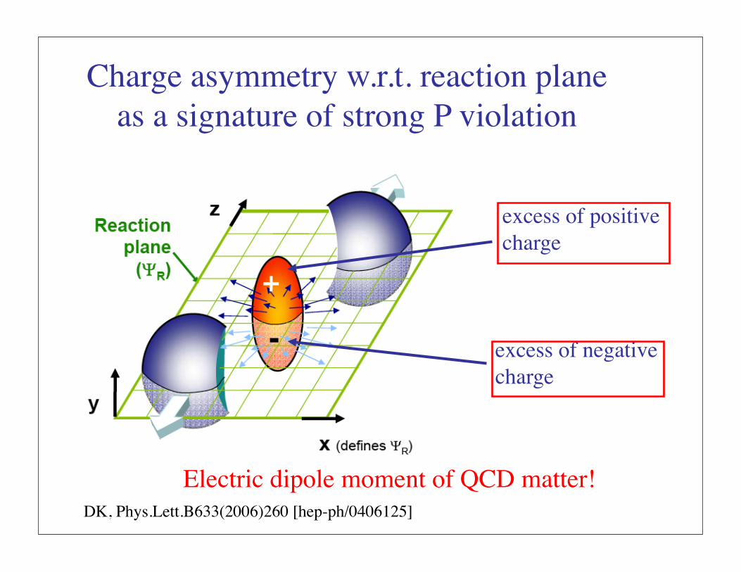
excess of positivecharge

excess of negativecharge

Electric dipole moment of QCD matter!DK, Phys.Lett.B633(2006)260 [hep-ph/0406125]

Charge asymmetry w.r.t. reaction plane as a signature of strong P violation

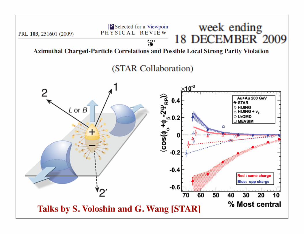
6Talks by S. Voloshin and G. Wang [STAR]

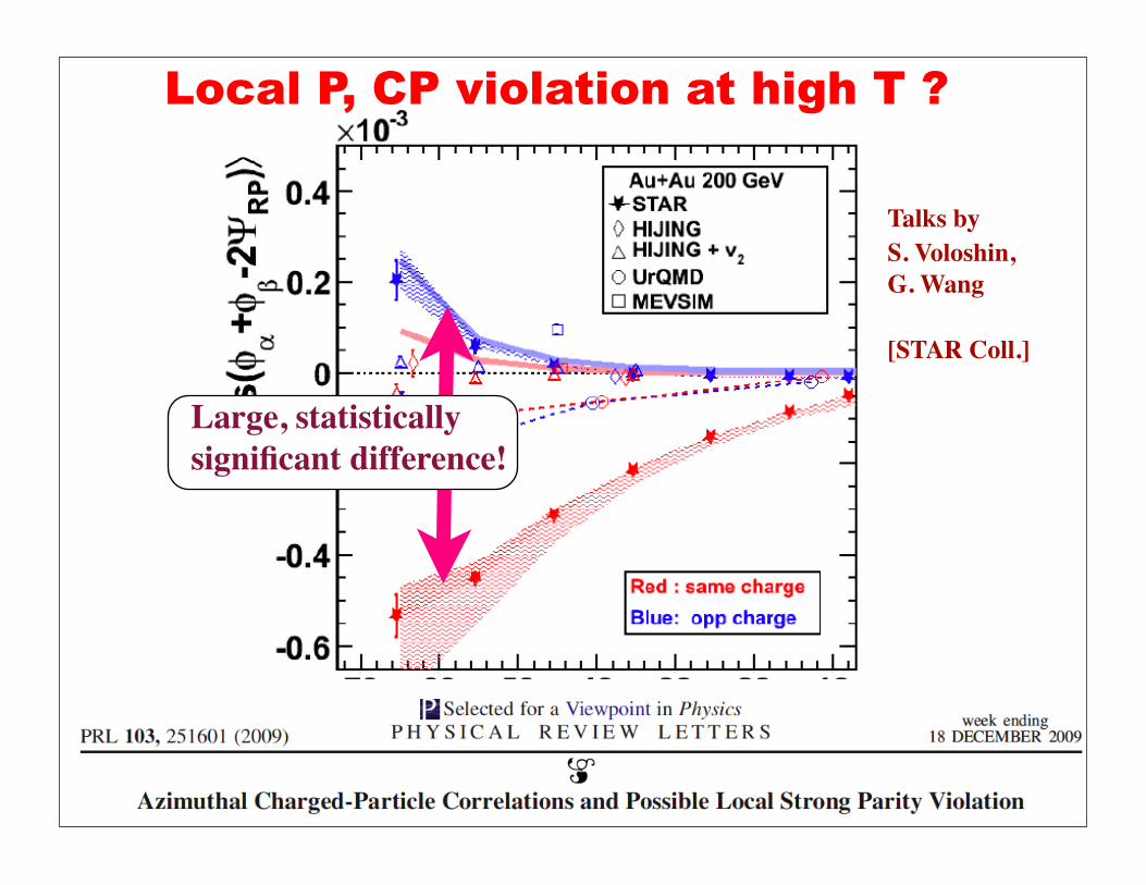
Local P, CP violation at high T ?

Large, statistically significant difference!

Talks byS. Voloshin,G. Wang

[STAR Coll.]

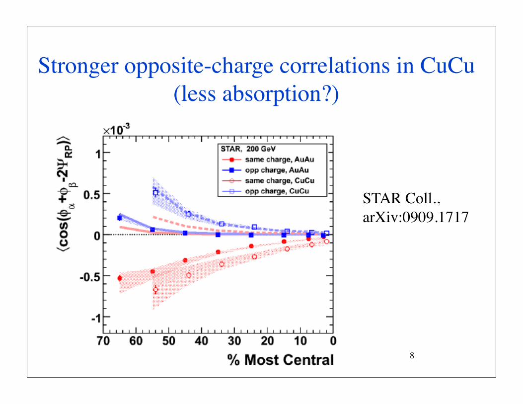
Stronger opposite-charge correlations in CuCu(less absorption?)

8

STAR Coll.,arXiv:0909.1717

-1 -0.5 0 0.5 10.995

1

1.005

1.01 Data 0-5% 0.4<pT<0.7 unreflected reflectedFast Sim (with decay)

a1=0.04a1=0.033a1=0.02

PHENIX Preliminary

Cp

S!

The PHENIX resulttalk by N. Ajitanand, Dec 17

9

-1 -0.5 0 0.5 10.995

1

1.005

1.01 Data 20-30% 0.4<pT<0.7 unreflected reflectedFast Simulator (with decay)

a1=0.065a1=0.055a1=0.04

PHENIX Preliminary

Cp

S!

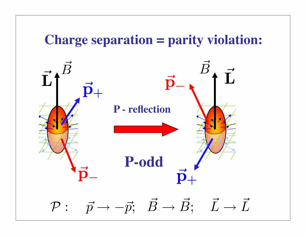
!B !B

P : !p! "!p; !B ! !B; !L! !L

P - reflection

P-odd

Charge separation = parity violation:

Analogy to P violation in weak interactions

C.S. Wu, 1912-1997

BUT:the sign ofthe asymmetryfluctuates event by event

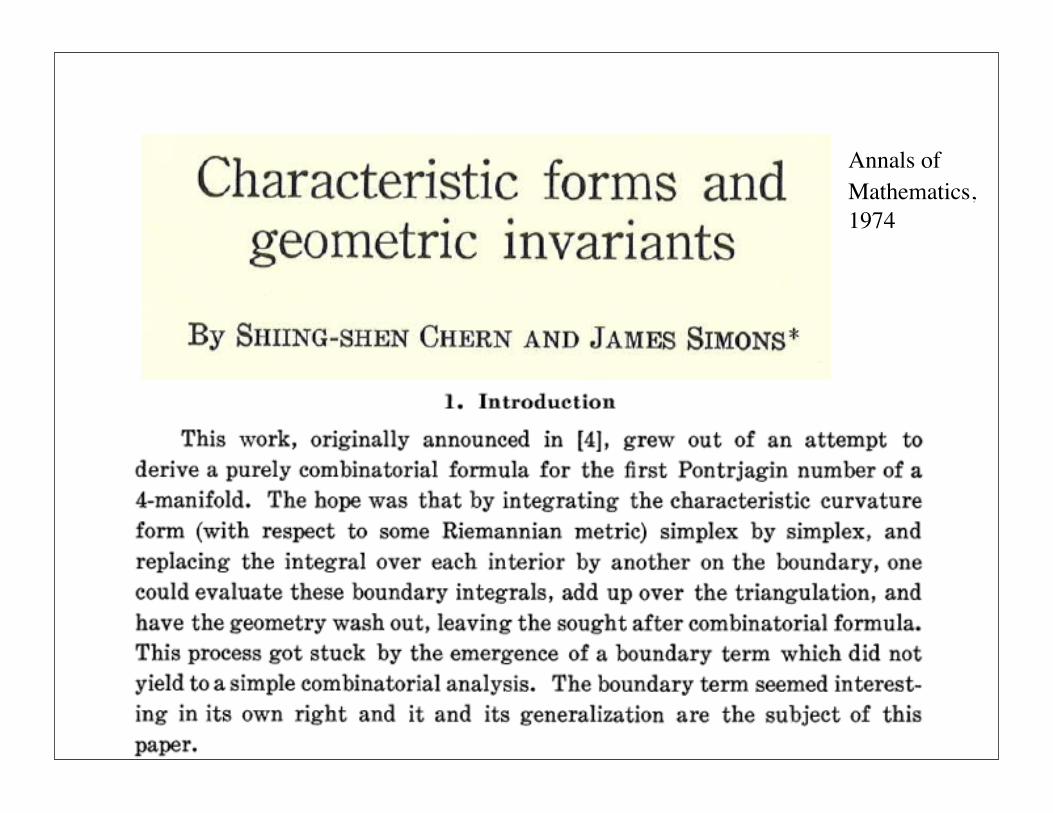
Annals of Mathematics, 1974

Chern-Simons forms

What does it mean for a gauge theory?

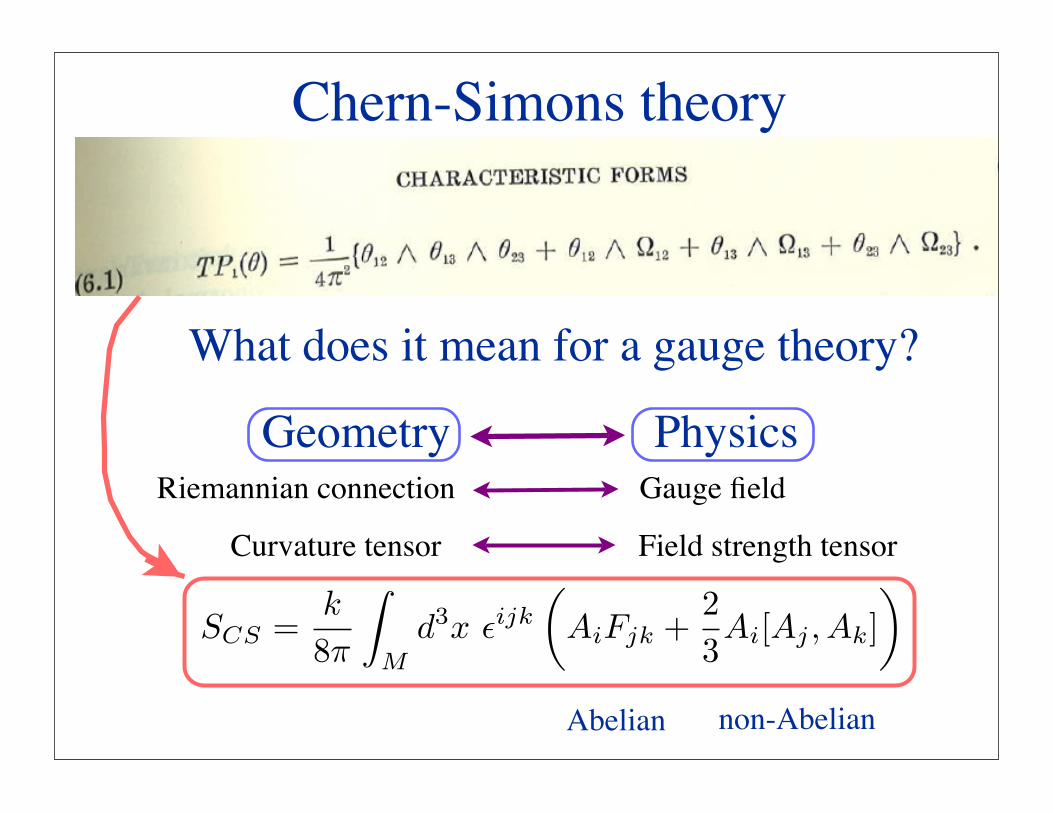
Chern-Simons theory

What does it mean for a gauge theory?

Riemannian connection

Curvature tensor Field strength tensor

Gauge fieldPhysicsGeometry

SCS =k

8!

!

Md3x "ijk

"AiFjk +

23Ai[Aj , Ak]

#

Abelian non-Abelian

Remarkable novel properties:

gauge invariant, up to a boundary term

topological - does not depend on the metric, knows only about the topology of space-time M

when added to Maxwell action, induces a mass for the gauge boson - different from the Higgs mechanism!

breaks Parity invariance

Chern-Simons theory

SCS =k

8!

!

Md3x "ijk

"AiFjk +

23Ai[Aj , Ak]

#

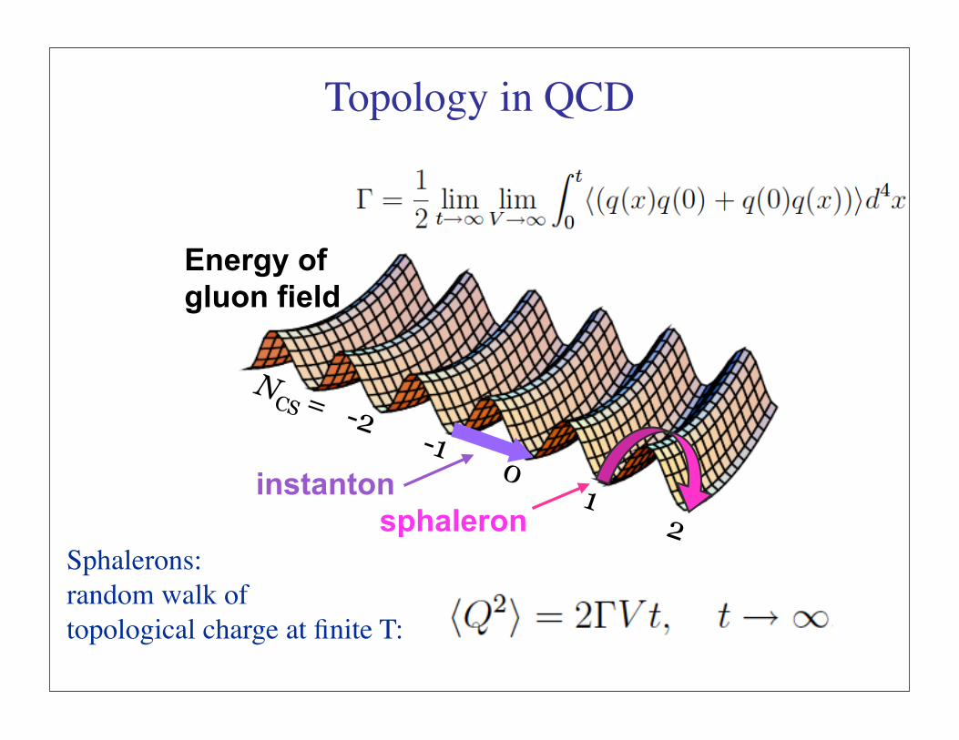
NCS = -2 -1 0 1 2

instanton

sphaleron

Energy of

gluon field

16

Topology in QCD

Sphalerons:random walk of topological charge at finite T:

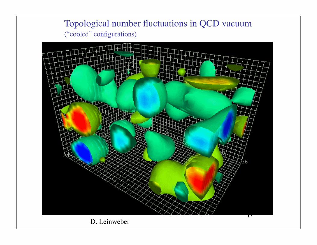
17D. Leinweber

Topological number fluctuations in QCD vacuum(“cooled” configurations)

18

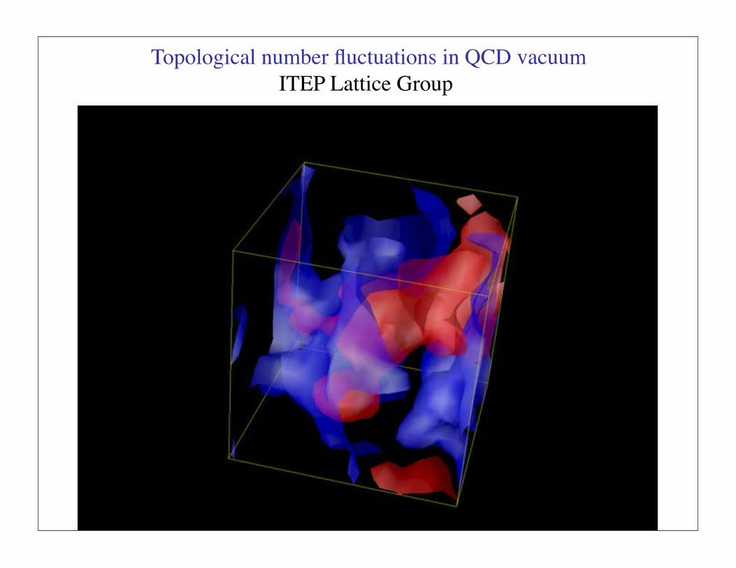
Topological number fluctuations in QCD vacuum ITEP Lattice Group

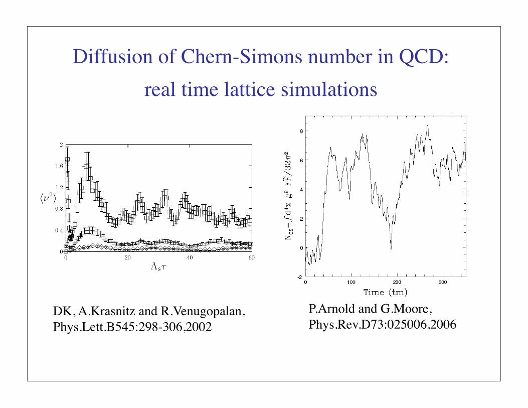
DK, A.Krasnitz and R.Venugopalan,Phys.Lett.B545:298-306,2002

P.Arnold and G.Moore,Phys.Rev.D73:025006,2006

Diffusion of Chern-Simons number in QCD: real time lattice simulations

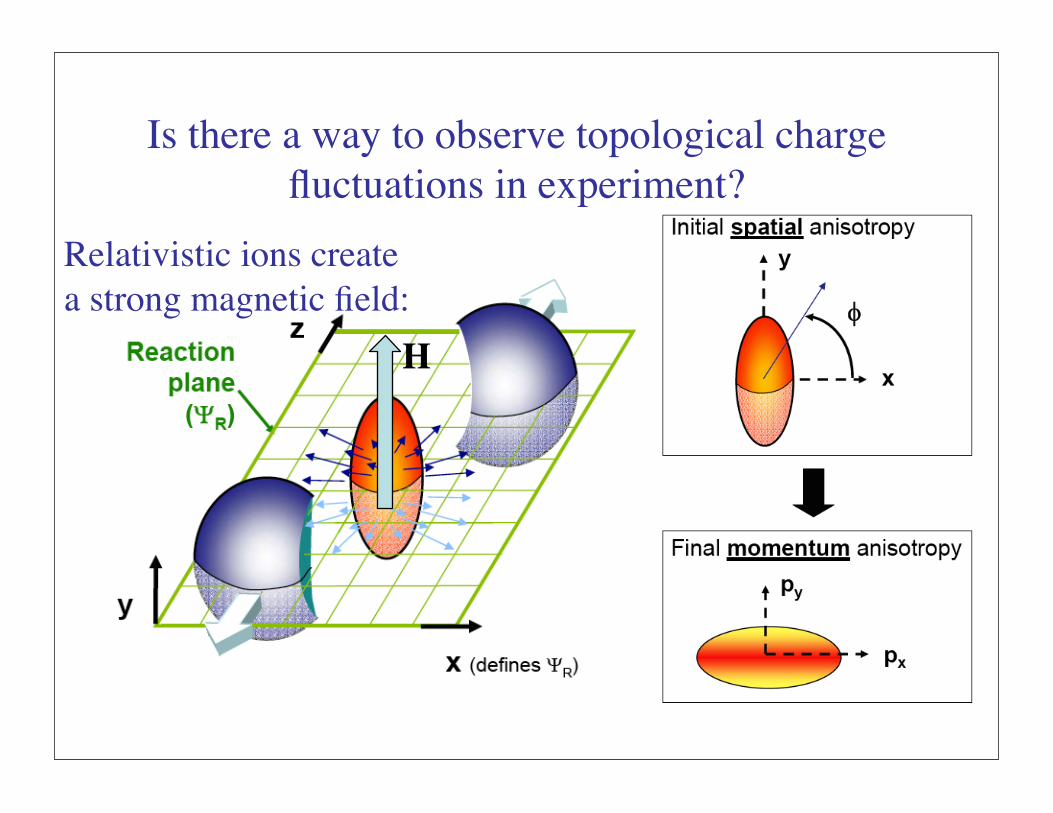
Is there a way to observe topological charge fluctuations in experiment?

Relativistic ions createa strong magnetic field:

H

46

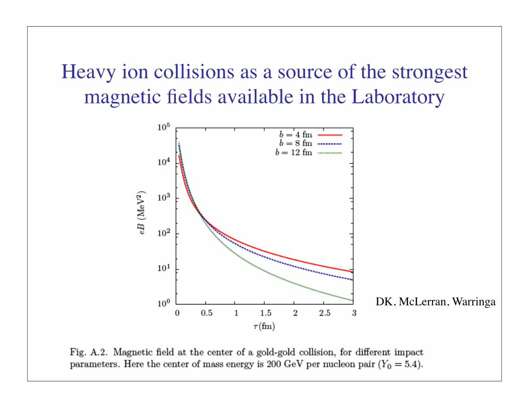
Heavy ion collisions as a source of the strongest magnetic fields available in the Laboratory

DK, McLerran, Warringa

47

Heavy ion collisions: the strongest magnetic field ever achieved in the laboratory

The situation is di!erent if the field ! = !("x, t) varies in space-time.Indeed, in this case we have

! ˜F µ!Fµ! = !#µJµCS = #µ [!Jµ

CS]! #µ!JµCS. (16)

The first term on r.h.s. is again a full derivative and can be omitted; intro-ducing notation

Pµ = #µ! = (M, "P ) (17)

we can re-write the Lagrangian (12) in the following form:

LMCS = !1

4F µ!Fµ! ! AµJ

µ +c

4PµJ

µCS. (18)

Since ! is a pseudo-scalar field, Pµ is a pseudo-vector; as is clear from (18),it plays a role of the potential coupling to the Chern-Simons current (15).However, unlike the vector potential Aµ, Pµ is not a dynamical variable andis a pseudo-vector that is fixed by the dynamics of chiral charge – in our case,determined by the fluctuations of topological charge in QCD.

In (3+1) space-time dimensions, the pseudo-vector Pµ selects a directionin space-time and thus breaks the Lorentz and rotational invariance: thetemporal component M breaks the invariance w.r.t. Lorentz boosts, whilethe spatial component "P picks a certain direction in space. On the otherhand, in (2 + 1) dimensions there is no need for the spatial component "Psince the Chern-Simons current (15) in this case reduces to the pseudo-scalarquantity $!"#A!F"#, so the last term in (18) takes the form

"L = c M$!"#A!F"#. (19)

This term is Lorentz-invariant although it still breaks parity. In other words,in (2+1) dimensions the vector "P can be chosen as a 3-vector pointing in thedirection of an ”extra dimension” orthogonal to the plane of the two spatialdimensions. This illustrates an important di!erence between the roles playedby the Chern-Simons term in even and odd number of space-time dimensions.It is well-known that the term (19) leads to a gauge-invariant mass of thephoton; we will also see that it plays an important role in the Hall e!ect.

4.2. Maxwell-Chern-Simons equationsLet us write down the Euler-Lagrange equations of motion that follow

from the Lagrangian (18),(15) (Maxwell-Chern-Simons equations):

#µFµ! = J! ! PµF

µ! . (20)

5

4. Topology-induced e!ects in electrodynamics:Maxwell-Chern-Simons theory

4.1. The Lagrangian

Let us begin by coupling the theory (1) to electromagnetism; the resultingtheory possesses SU(3)! U(1) gauge symmetry:

LQCD+QED = "1

4Gµ!

" G"µ! +!

f

!f [i"µ(#µ " igA"µt" " iqfAµ)"mf ] !f"

" $

32%2g2Gµ!

" G"µ! "1

4F µ!Fµ! , (11)

where Aµ and Fµ! are the electromagnetic vector potential and the corre-sponding field strength tensor, and qf are the electric charges of the quarks.

Let us discuss the electromagnetic sector of the theory (11). Electromag-netic fields will couple to the electromagnetic currents Jµ =

"f qf !f"µ!f .

In addition, the term (10) will induce through the quark loop the coupling ofFF to the QCD topological charge. We will introduce an e!ective pseudo-scalar field $ = $(&x, t) (playing the role of the axion field) and write downthe resulting e!ective Lagrangian as

LMCS = "1

4F µ!Fµ! " AµJ

µ " c

4$ ˜F µ!Fµ! , (12)

wherec =

!

f

q2fe

2/(2%2). (13)

check the coe"cient and sign of AµJµ

This is the Lagrangian of Maxwell-Chern-Simons, or axion, electrodynam-ics. If $ is a constant, then the last term in (12) represents a full divergence

˜F µ!Fµ! = #µJµCS (14)

of the Chern-Simons current

JµCS = 'µ!#$A!F#$, (15)

which is the Abelian analog of (4). Being a full divergence, this term doesnot a!ect the equations of motion and does not a!ect the electrodynamics.

4

The situation is di!erent if the field ! = !("x, t) varies in space-time.Indeed, in this case we have

! ˜F µ!Fµ! = !#µJµCS = #µ [!Jµ

CS]! #µ!JµCS. (16)

The first term on r.h.s. is again a full derivative and can be omitted; intro-ducing notation

Pµ = #µ! = (M, "P ) (17)

we can re-write the Lagrangian (12) in the following form:

LMCS = !1

4F µ!Fµ! ! AµJ

µ +c

4PµJ

µCS. (18)

Since ! is a pseudo-scalar field, Pµ is a pseudo-vector; as is clear from (18),it plays a role of the potential coupling to the Chern-Simons current (15).However, unlike the vector potential Aµ, Pµ is not a dynamical variable andis a pseudo-vector that is fixed by the dynamics of chiral charge – in our case,determined by the fluctuations of topological charge in QCD.

In (3+1) space-time dimensions, the pseudo-vector Pµ selects a directionin space-time and thus breaks the Lorentz and rotational invariance: thetemporal component M breaks the invariance w.r.t. Lorentz boosts, whilethe spatial component "P picks a certain direction in space. On the otherhand, in (2 + 1) dimensions there is no need for the spatial component "Psince the Chern-Simons current (15) in this case reduces to the pseudo-scalarquantity $!"#A!F"#, so the last term in (18) takes the form

"L = c M$!"#A!F"#. (19)

This term is Lorentz-invariant although it still breaks parity. In other words,in (2+1) dimensions the vector "P can be chosen as a 3-vector pointing in thedirection of an ”extra dimension” orthogonal to the plane of the two spatialdimensions. This illustrates an important di!erence between the roles playedby the Chern-Simons term in even and odd number of space-time dimensions.It is well-known that the term (19) leads to a gauge-invariant mass of thephoton; we will also see that it plays an important role in the Hall e!ect.

4.2. Maxwell-Chern-Simons equationsLet us write down the Euler-Lagrange equations of motion that follow

from the Lagrangian (18),(15) (Maxwell-Chern-Simons equations):

#µFµ! = J! ! PµF

µ! . (20)

5

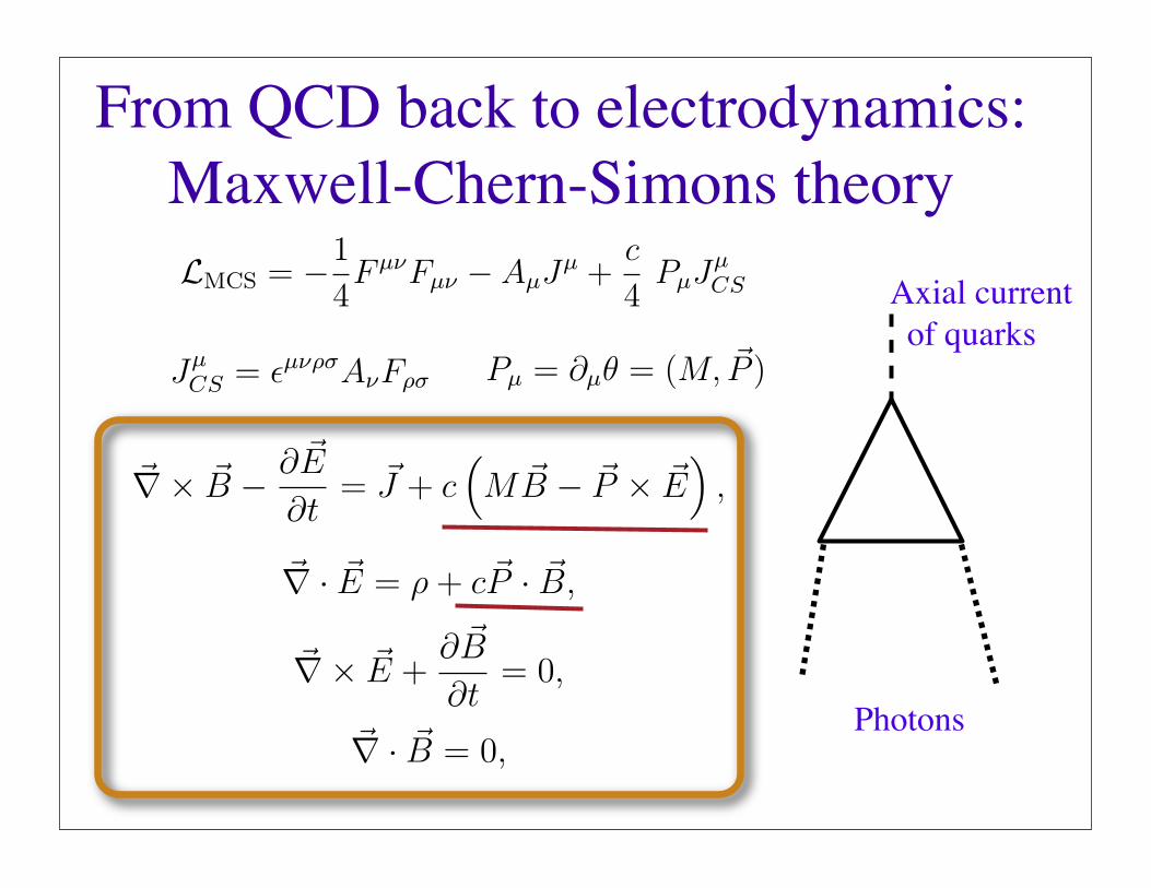
From QCD back to electrodynamics:Maxwell-Chern-Simons theory

Axial current of quarks

Photons

The first pair of Maxwell equations (which is a consequence of the fact thatthe fields are expressed through the vector potential) is not modified:

!µFµ! = J! . (21)

It is convenient to write down these equations also in terms of the electric "Eand magnetic "B fields:

"!" "B # ! "E

!t= "J + c

!M "B # "P " "E

", (22)

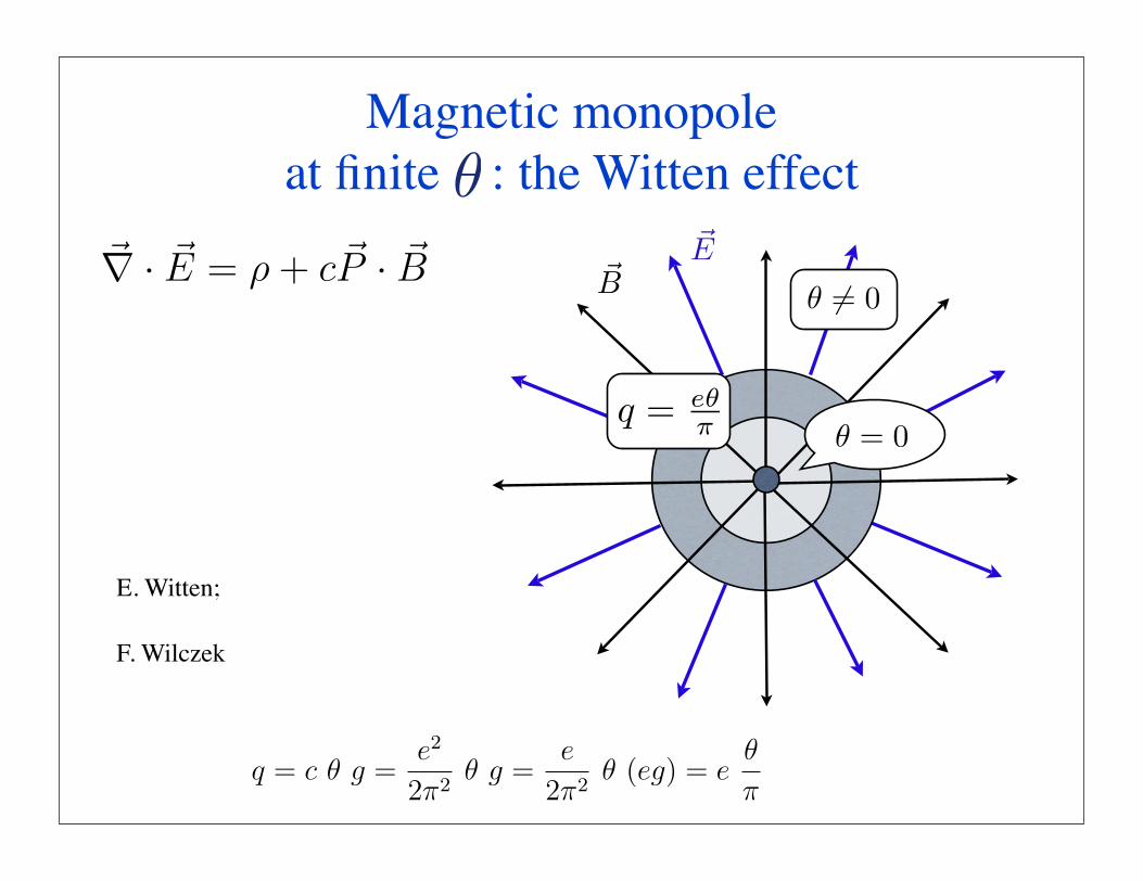
"! · "E = # + c"P · "B, (23)

"!" "E +! "B

!t= 0, (24)

"! · "B = 0, (25)

where (#, "J) are the electric charge and current densities. One can see thatthe presence of Chern-Simons term leads to essential modifications of theMaxwell theory. Let us look at a few known examples illustrating the dy-namics contained in Eqs(22),(23),(24),(25).

4.2.1. The Witten e!ectLet us consider, following Wilczek [10], a magnetic monopole in the pres-

ence of finite $ angle. In the core of the monopole $ = 0, and away fromthe monopole $ acquires a finite non-zero value – therefore within a finitedomain wall we have a non-zero "P = "!$ pointing radially outwards fromthe monopole. According to (23), the domain wall thus acquires a non-zerocharge density c"!$ · "B. An integral along "P (across the domain wall) yields#

dl !$/!l = $, and the integral over all directions of "P yields the total mag-netic flux !. By Gauss theorem, the flux is equal to the magnetic charge ofthe monopole g, and the total electric charge of the configuration is equal to

q = c $ g =e2

2%2$ g =

e

2%2$ (eg) = e

$

%, (26)

where we have used an explicit expression (13) for the coupling constant c,as well as the Dirac condition ge = 2% " integer.

6

!


!µFµ! = J! . (21)


"!" "B # ! "E

!t= "J + c

!M "B # "P " "E

", (22)

"! · "E = # + c"P · "B, (23)

"!" "E +! "B

!t= 0, (24)

"! · "B = 0, (25)





q = c $ g =e2

2%2$ g =

e

2%2$ (eg) = e

$

%, (26)


6

! != 0!B

!E

! = 0q = e!

"

Figure 1: Magnetic monopole at finite ! angle acquires an electric charge ! e!/" that islocalized on the domain wall where the value of ! changes from zero in the core of themonopole to some value ! "= 0 away from the monopole (the domain wall is shown by thegray ring) – the Witten e!ect.

4.2.2. Charge separation e!ectConsider now a configuration shown on Fig. where an external magnetic

field !B pierces a domain with " "= 0 inside; outside " = 0. Let us assume firstthat the field " is static, " = 0. Assuming that the field !B is perpendicularto the domain wall, we find from (23) that the upper domain wall acquiresthe charge density per unit area S of

!Q

S

"

up

= + c "B (27)

while the lower domain wall acquires the same in magnitude but opposite insign charge density !

Q

S

"

down

= # c "B (28)

7

Magnetic monopole at finite : the Witten effect


!µFµ! = J! . (21)


"!" "B # ! "E

!t= "J + c

!M "B # "P " "E

", (22)

"! · "E = # + c"P · "B, (23)

"!" "E +! "B

!t= 0, (24)

"! · "B = 0, (25)





q = c $ g =e2

2%2$ g =

e

2%2$ (eg) = e

$

%, (26)


6

E. Witten;

F. Wilczek


!µFµ! = J! . (21)


"!" "B # ! "E

!t= "J + c

!M "B # "P " "E

", (22)

"! · "E = # + c"P · "B, (23)

"!" "E +! "B

!t= 0, (24)

"! · "B = 0, (25)





q = c $ g =e2

2%2$ g =

e

2%2$ (eg) = e

$

%, (26)


6

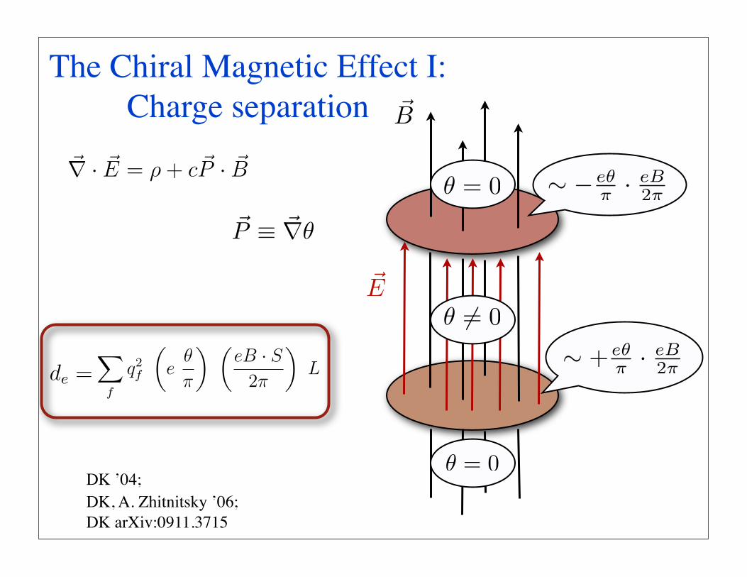
Assuming that the domain walls are thin compared to the distance L betweenthem, we find that the system possesses an electric dipole moment

de = c ! (B · S) L =!

f

q2f

"e

!

"

# "eB · S

2"

#L; (29)

in what follows we will for the brevity of notations put$

f q2f = 1; it is easy

to restore this factor in front of e2 when needed.

!B

!E

! + e!" · eB

2"

! " e!" · eB

2"

! != 0

! = 0

! = 0

Figure 2: Charge separation e!ect – domain walls that separate the region of ! != 0 fromthe outside vacuum with ! = 0 become charged in the presence of an external magneticfield, with the surface charge density " e!/" · eB/2". This induces an electric dipolemoment signaling P and CP violation.

Static electric dipole moment is a signature of P , T and CP violation (weassume that CPT invariance holds). The spatial separation of charge willinduce the corresponding electric field #E = c ! #B. The mixing of pseudo-vector magnetic field #B and the vector electric field #E signals violation of P ,T and CP invariances.

8

The Chiral Magnetic Effect I:Charge separation


de = c ! (B · S) L =!

f

q2f

"e

!

"

# "eB · S

2"

#L; (29)






8


de = c ! (B · S) L =!

f

q2f

"e

!

"

# "eB · S

2"

#L; (29)






8

DK ’04;DK, A. Zhitnitsky ’06;DK arXiv:0911.3715

!P ! !""

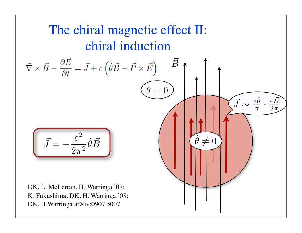
Note that this current directed along the magnetic field !B represents a P!,T ! and CP! phenomenon and of course is absent in the ”ordinary” Maxwellequations. Integrating the current density over time (assuming that the field!B is static) we find that when " changes from zero to some " "= 0, this resultsin a separation of charge and the electric dipole moment (29).

!B

! = 0

! != 0

!J ! e!" · e #B

2"

Figure 3: The chiral magnetic e!ect – inside a domain with ! "= 0 an external magneticfield induces an electric current "J # e!/# · e "B/2#. ! "= 0 indicates the change of the chiralcharge inducing an asymmetry between the left– and right– handed fermions inside thedomain. Note that the current "J # "B is absent in Maxwell electrodynamics.

Let us discuss the meaning of formula (30) in more detail. To do this,let us consider the work done by the electric current; to obtain the work perunit time – the power P – we multiply both sides of (30) by the electric field!E and integrate them over the volume (as before, we assume that " does notdepend on spatial coordinates):

P =

!d3x !J · !E = !"

e2

2#2

!d3x !E · !B = !" Q5, (31)

10

The chiral magnetic effect II:chiral induction

DK, L. McLerran, H. Warringa ’07;K. Fukushima, DK, H. Warringa ’08;DK, H.Warringa arXiv:0907.5007

!J = ! e2

2"2# !B

Right

µR

Left

µLµL ! µR = 2 !

Figure 4: Dirac cones of the left and right fermions. In the presence of the changing chiralcharge there is an asymmetry between the Fermi energies of left and right fermions µL

and µR: µL ! µR = 2µ5 = 2!.

momentum, and we are dealing with the right fermions. Likewise, the nega-tive fermions will be leftt-handed. After time t, the positive (right) fermionswill increase their Fermi momentum to pF

R = eEt, and the negative (left) willhave their Fermi momentum decreased to pF

L = !pFR. The one-dimensional

density of states along the axis z that we choose parallel to the direction offields !E and !B is given by dNR/dz = pF

R/2". In the transverse direction, themotion of fermions is quantized as they populate Landau levels in the mag-netic field. The transverse density of Landau levels is d2NR/dxdy = eB/2".Therefore the density of right fermions increases per unit time as

d4NR

dt dV=

e2

(2")2!E · !B. (35)

The density of left fermions decreases with the same rate, d4NL/dt dV =

12

What powers the CME current?

“Numerical evidence for chiral magnetic effect in lattice gauge theory”,P. Buividovich, M. Chernodub, E. Luschevskaya, M. Polikarpov, ArXiv 0907.0494; PRD’09

SU(2) quenched, Q = 3; Electric charge density (H) - Electric charge density (H=0)

Red - positive chargeBlue - negative charge

“Chiral magnetic effect in 2+1 flavor QCD+QED”,M. Abramczyk, T. Blum, G. Petropoulos, R. Zhou, ArXiv 0911.1348;Columbia-Bielefeld-RIKEN-BNL

2+1 flavor Domain Wall Fermions, fixed topological sectors, 16^3 x 8 lattice

Red - positive chargeBlue - negative charge

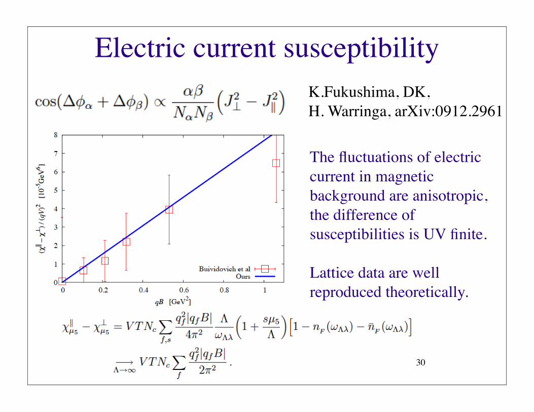
Electric current susceptibility

30

K.Fukushima, DK,H. Warringa, arXiv:0912.2961

The fluctuations of electric current in magnetic background are anisotropic, the difference of susceptibilities is UV finite.

Lattice data are well reproduced theoretically.

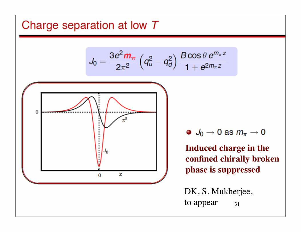
31

DK, S. Mukherjee, to appear

Induced charge in the confined chirally broken phase is suppressed

2

asymmetry can be investigated experimentally using theobservables proposed in Ref. [24]. Preliminary data of theSTAR collaboration has been presented in Refs. [25, 26].Implications of the Chiral Magnetic E!ect on astrophys-ical phenomena have recently been discussed in Ref. [27];another astrophysical implication can be found in [28].

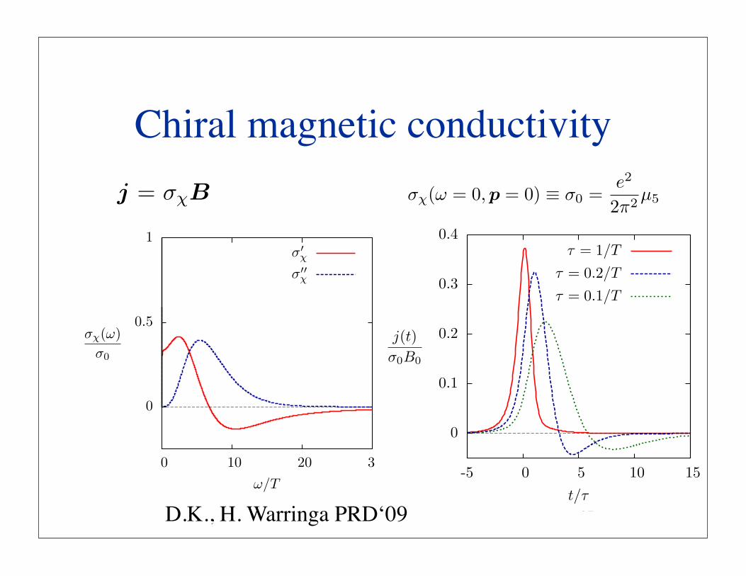
A system of massless fermions with nonzero chiralitycan be described by a chiral chemical potential µ5 whichcouples to the zero component of the axial vector currentin the Lagrangian. The induced current in such situa-tion can be written as j = !!B, where !! is the ChiralMagnetic conductivity. For constant and homogeneousmagnetic fields its value is determined by the electro-magnetic axial anomaly and for one flavor and one colorequal to [22, 29, 30] (see also [31])

!!(" = 0,p = 0) ! !0 =e2

2#2µ5, (2)

where " and p denote frequency and momentum respec-tively, and e equals the unit charge. For a finite numberof colors Nc and flavors f one has to multiply this resultby Nc

!f q2

f where qf denotes the charge of a quark inunits of e. The generation of currents due to the anomalyin background fields or rotating systems is also discussedin related contexts in Refs. [31–35].

For constant magnetic fields which are inhomogeneousin the plane transverse to the field one finds that the totalcurrent J along B equals [22],

J = e"e"

2#

#Lzµ5

#, (3)

where Lz is the length of the system in the z-directionand the flux " is equal to the integral of the magneticfield over the transverse plane,

" =$

d2x B(x, y). (4)

The floor function "x# is the largest integer smaller thanx. The quantity "e"/(2#)# in Eq. (3) is equal to thenumber of zero modes in the magnetic field [36].

To compute the current generated by a configurationof specific topological charge, one should express µ5 interms of the chirality N5. By using the anomaly relationone can then relate N5 to the topological charge. This isdiscussed in detail in Ref. [22].

The aim of this paper is to study how a system withconstant nonzero chirality responds to a time dependentmagnetic field. This is interesting for phenomenologysince the magnetic field produced with heavy ion colli-sions depends strongly on time. To obtain the inducedcurrent in a time-dependent magnetic field, we will com-pute the Chiral Magnetic conductivity for nonzero fre-quencies and nonzero momenta using linear response the-ory. We will compute the leading order conductivity andleave the inclusion of corrections due to photon and orgluon exchange for future work. In leading order the Chi-ral Magnetic conductivity for an electromagnetic plasma

and quark gluon plasma are equal (up to a trivial factorof Nc). Since we do not take into account higher ordercorrections, some of our results for QCD will only bea good approximation in the limit of very high tempera-tures where the strong coupling constant $s is su#cientlysmall.

We will take the metric gµ" = diag(+,$,$,$).The gamma matrices in the complete article satisfy{%µ, %"} = 2gµ" . We will use the notation p for boththe four-vector pµ = (p0,p) and the length of a three-vector p = |p|.

II. KUBO FORMULA FOR CHIRALMAGNETIC CONDUCTIVITY

For small magnetic fields, the induced vector currentcan be found using the Kubo formula. This formula tellsus that to first order in the time-dependent perturbation,the induced vector current is equal to retarded correlatorof the vector current with the perturbation evaluated inequilibrium. More explicitly, one finds that

%jµ(x)& =$

d4x! $µ"R (x, x!)A"(x!), (5)

where jµ(x) = e&(x)%µ&(x) and the retarded responsefunction $µ"

R is given by

$µ"R (x, x!) = i%[jµ(x), j"(x!)]&'(t$ t!). (6)

The equilibrium Hamiltonian is invariant under trans-lations in time and space, therefore we can use that$µ"

R (x, x!) = $µ"R (x$x!). Let us take a vector field of the

following specific form A"(x) = A"(p)e"ipx. The Kuboformula now becomes,

%jµ(x)& = $µ"R (p)A"(p)e"ipx, (7)

where

$µ"R (p) =

$d4x eipx$µ"

R (x). (8)

In order to compute the Chiral Magnetic conductiv-ity we will take a time-dependent magnetic field pointingin the z-direction. Because of Faraday’s law (! ' E =$(B/(t), such time-dependent magnetic field comes al-ways together with a perpendicular electric field. Letus choose a gauge such that the only component of thevector field that is non-vanishing is Ay. Then Bz(x) =(xAy(x) so that Bz(p) = ip1A2(p). Using Eq. (7) wefind that the induced vector current in the direction ofthe magnetic field can now be written as

%jz(x)& = !!(p)Bz(p)e"ipx, (9)

where the Chiral Magnetic conductivity equals

!!(p) =1

ip1$23

R (p) =1

2ipi$jk

R (p))ijk. (10)

2

asymmetry can be investigated experimentally using theobservables proposed in Ref. [24]. Preliminary data of theSTAR collaboration has been presented in Refs. [25, 26].Implications of the Chiral Magnetic E!ect on astrophys-ical phenomena have recently been discussed in Ref. [27];another astrophysical implication can be found in [28].

A system of massless fermions with nonzero chiralitycan be described by a chiral chemical potential µ5 whichcouples to the zero component of the axial vector currentin the Lagrangian. The induced current in such situa-tion can be written as j = !!B, where !! is the ChiralMagnetic conductivity. For constant and homogeneousmagnetic fields its value is determined by the electro-magnetic axial anomaly and for one flavor and one colorequal to [22, 29, 30] (see also [31])

!!(" = 0,p = 0) ! !0 =e2

2#2µ5, (2)

where " and p denote frequency and momentum respec-tively, and e equals the unit charge. For a finite numberof colors Nc and flavors f one has to multiply this resultby Nc

!f q2

f where qf denotes the charge of a quark inunits of e. The generation of currents due to the anomalyin background fields or rotating systems is also discussedin related contexts in Refs. [31–35].

For constant magnetic fields which are inhomogeneousin the plane transverse to the field one finds that the totalcurrent J along B equals [22],

J = e"e"

2#

#Lzµ5

#, (3)

where Lz is the length of the system in the z-directionand the flux " is equal to the integral of the magneticfield over the transverse plane,

" =$

d2x B(x, y). (4)

The floor function "x# is the largest integer smaller thanx. The quantity "e"/(2#)# in Eq. (3) is equal to thenumber of zero modes in the magnetic field [36].

To compute the current generated by a configurationof specific topological charge, one should express µ5 interms of the chirality N5. By using the anomaly relationone can then relate N5 to the topological charge. This isdiscussed in detail in Ref. [22].

The aim of this paper is to study how a system withconstant nonzero chirality responds to a time dependentmagnetic field. This is interesting for phenomenologysince the magnetic field produced with heavy ion colli-sions depends strongly on time. To obtain the inducedcurrent in a time-dependent magnetic field, we will com-pute the Chiral Magnetic conductivity for nonzero fre-quencies and nonzero momenta using linear response the-ory. We will compute the leading order conductivity andleave the inclusion of corrections due to photon and orgluon exchange for future work. In leading order the Chi-ral Magnetic conductivity for an electromagnetic plasma

and quark gluon plasma are equal (up to a trivial factorof Nc). Since we do not take into account higher ordercorrections, some of our results for QCD will only bea good approximation in the limit of very high tempera-tures where the strong coupling constant $s is su#cientlysmall.

We will take the metric gµ" = diag(+,$,$,$).The gamma matrices in the complete article satisfy{%µ, %"} = 2gµ" . We will use the notation p for boththe four-vector pµ = (p0,p) and the length of a three-vector p = |p|.

II. KUBO FORMULA FOR CHIRALMAGNETIC CONDUCTIVITY

For small magnetic fields, the induced vector currentcan be found using the Kubo formula. This formula tellsus that to first order in the time-dependent perturbation,the induced vector current is equal to retarded correlatorof the vector current with the perturbation evaluated inequilibrium. More explicitly, one finds that

%jµ(x)& =$

d4x! $µ"R (x, x!)A"(x!), (5)

where jµ(x) = e&(x)%µ&(x) and the retarded responsefunction $µ"

R is given by

$µ"R (x, x!) = i%[jµ(x), j"(x!)]&'(t$ t!). (6)

The equilibrium Hamiltonian is invariant under trans-lations in time and space, therefore we can use that$µ"

R (x, x!) = $µ"R (x$x!). Let us take a vector field of the

following specific form A"(x) = A"(p)e"ipx. The Kuboformula now becomes,

%jµ(x)& = $µ"R (p)A"(p)e"ipx, (7)

where

$µ"R (p) =

$d4x eipx$µ"

R (x). (8)

In order to compute the Chiral Magnetic conductiv-ity we will take a time-dependent magnetic field pointingin the z-direction. Because of Faraday’s law (! ' E =$(B/(t), such time-dependent magnetic field comes al-ways together with a perpendicular electric field. Letus choose a gauge such that the only component of thevector field that is non-vanishing is Ay. Then Bz(x) =(xAy(x) so that Bz(p) = ip1A2(p). Using Eq. (7) wefind that the induced vector current in the direction ofthe magnetic field can now be written as

%jz(x)& = !!(p)Bz(p)e"ipx, (9)

where the Chiral Magnetic conductivity equals

!!(p) =1

ip1$23

R (p) =1

2ipi$jk

R (p))ijk. (10)

7

!!!!

!!!

"/T

!!(")!0

3020100

1

0.5

0

FIG. 3: Real (red, solid) and imaginary (blue, dashed) part ofthe leading order normalized Chiral Magnetic conductivity athigh temperatures (T > µ5) for homogeneous magnetic fields(p = 0). At ! = 0 the normalized conductivity is equal to 1.

conductivity drops from !0 at " = 0 to !0/3 just awayfrom " = 0.

D. Discussion

We display the real and imaginary part for T = 0, p =0.1µ5 and µ = 0 in Fig. 1. As was argued at the end ofthe previous subsection, it can be seen in this figure thatthe real part of the Chiral Magnetic conductivity dropsfrom !0 at " = 0 to !0/3 just away from " = 0. Alsothe resonance at " = 2µ5 is clearly visible. The width ofthe imaginary part at the resonance is equal to 2p. Thereal part of the conductivity becomes negative above theresonance frequency. This is a typical resonance behaviorand implies that when the imaginary part vanishes theresponse is 180 degrees out of phase with the appliedmagnetic field.

In Fig. 2 we display the real and imaginary part forT = 0, p = 0.1µ5 and µ = 1.5µ5. In this case there areresonances at " = 5µ5 and " = µ5. Equation (45) showsthat the imaginary part is proportional to "2, thereforethe second resonance at " = 5µ5 is much stronger thanthe first one at " = µ5. Because the second resonanceis due to the right-handed modes, and the first one dueto left-handed, the contribution of the second resonancehas opposite sign to the first resonance.

The real and imaginary part of the Chiral Magneticconductivity at high temperatures (T > µ5) are displayedin Fig. 3. This figure is the most relevant for QCD atvery high temperatures, since then loop corrections willbe small. As argued in the previous subsection it can beseen in the figure that the real part of the conductivitydrops from !0 at " = 0 to !0/3 just away from " = 0.

Let us now study the induced current in a magnetic

FIG. 4: Induced current in time-dependent magnetic field,Eq. (49), as a function of time, at very high temperature.The results are plotted for di!erent values of the characteristictime scale " of the magnetic field.

field of the form created during heavy ion collisions. Forsimplicity we approximate the two colliding nuclei bypoint like particles like in Ref. [19]. This gives a reason-able approximation to the more accurate methods dis-cussed in Refs. [17, 18] and is most reliable for large im-pact parameters. The magnetic field at the center of thecollision can then be written as

B(t) =1

[1 + (t/#)2]3/2B0, (49)

with # = b/(2 sinhY ) and eB0 = 8Z$EM sinhY/b2. Hereb denotes the impact parameter, Z the charge of the nu-cleus, and Y the beam rapidity. For Gold-Gold (Z = 79)collisions at 100 GeV per nucleon one has Y = 5.36. Attypical large impact parameters (say b = 10 fm) one findseB0 ! 1.9 " 105 MeV2 and # = 0.05 fm/c. For 31 GeVper nucleon (Y = 4.19) Gold-Gold collsions one finds atb = 10 fm, eB0 ! 5.9 " 104 MeV2 and # = 0.15 fm/c.The Fourier transform of Eq. (49) equals

B(") = 2#2|"|K1(# |"|)B0, (50)

where K1(z) denotes the first-order modified Bessel func-tion of the second kind.

For illustration purposes we will assume that our mag-netic field is (unlike in heavy ion collisions) homogeneous.The induced current can be found by applying Eq. (19).We display the induced current in the magnetic field ofEq. (49) in a system with nonzero chirality at very hightemperatures in Fig. 4. The induced current is plotted asa function of time for three di!erent characteristic timescales # of the magnetic field.

In any general decaying magnetic field, the only rel-evant frequencies are the ones which are smaller thanof order the inverse life-time of the magnetic field, " <!

Chiral magnetic conductivity

32

7

FIG. 3: Real (red, solid) and imaginary (blue, dashed) part ofthe leading order normalized Chiral Magnetic conductivity athigh temperatures (T > µ5) for homogeneous magnetic fields(p = 0). At ! = 0 the normalized conductivity is equal to 1.

conductivity drops from !0 at " = 0 to !0/3 just awayfrom " = 0.

D. Discussion

We display the real and imaginary part for T = 0, p =0.1µ5 and µ = 0 in Fig. 1. As was argued at the end ofthe previous subsection, it can be seen in this figure thatthe real part of the Chiral Magnetic conductivity dropsfrom !0 at " = 0 to !0/3 just away from " = 0. Alsothe resonance at " = 2µ5 is clearly visible. The width ofthe imaginary part at the resonance is equal to 2p. Thereal part of the conductivity becomes negative above theresonance frequency. This is a typical resonance behaviorand implies that when the imaginary part vanishes theresponse is 180 degrees out of phase with the appliedmagnetic field.

In Fig. 2 we display the real and imaginary part forT = 0, p = 0.1µ5 and µ = 1.5µ5. In this case there areresonances at " = 5µ5 and " = µ5. Equation (45) showsthat the imaginary part is proportional to "2, thereforethe second resonance at " = 5µ5 is much stronger thanthe first one at " = µ5. Because the second resonanceis due to the right-handed modes, and the first one dueto left-handed, the contribution of the second resonancehas opposite sign to the first resonance.

The real and imaginary part of the Chiral Magneticconductivity at high temperatures (T > µ5) are displayedin Fig. 3. This figure is the most relevant for QCD atvery high temperatures, since then loop corrections willbe small. As argued in the previous subsection it can beseen in the figure that the real part of the conductivitydrops from !0 at " = 0 to !0/3 just away from " = 0.

Let us now study the induced current in a magnetic

! = 0.1/T

! = 0.2/T

! = 1/T

t/!

j(t)"0B0

151050-5

0.4

0.3

0.2

0.1

0

FIG. 4: Induced current in time-dependent magnetic field,Eq. (49), as a function of time, at very high temperature.The results are plotted for di!erent values of the characteristictime scale " of the magnetic field.

field of the form created during heavy ion collisions. Forsimplicity we approximate the two colliding nuclei bypoint like particles like in Ref. [19]. This gives a reason-able approximation to the more accurate methods dis-cussed in Refs. [17, 18] and is most reliable for large im-pact parameters. The magnetic field at the center of thecollision can then be written as

B(t) =1

[1 + (t/#)2]3/2B0, (49)

with # = b/(2 sinhY ) and eB0 = 8Z$EM sinhY/b2. Hereb denotes the impact parameter, Z the charge of the nu-cleus, and Y the beam rapidity. For Gold-Gold (Z = 79)collisions at 100 GeV per nucleon one has Y = 5.36. Attypical large impact parameters (say b = 10 fm) one findseB0 ! 1.9 " 105 MeV2 and # = 0.05 fm/c. For 31 GeVper nucleon (Y = 4.19) Gold-Gold collsions one finds atb = 10 fm, eB0 ! 5.9 " 104 MeV2 and # = 0.15 fm/c.The Fourier transform of Eq. (49) equals

B(") = 2#2|"|K1(# |"|)B0, (50)

where K1(z) denotes the first-order modified Bessel func-tion of the second kind.

For illustration purposes we will assume that our mag-netic field is (unlike in heavy ion collisions) homogeneous.The induced current can be found by applying Eq. (19).We display the induced current in the magnetic field ofEq. (49) in a system with nonzero chirality at very hightemperatures in Fig. 4. The induced current is plotted asa function of time for three di!erent characteristic timescales # of the magnetic field.

In any general decaying magnetic field, the only rel-evant frequencies are the ones which are smaller thanof order the inverse life-time of the magnetic field, " <!

D.K., H. Warringa PRD‘09

Holographic chiral magnetic conductivity:the strong coupling regime

33H.-U. Yee, arXiv:0908.4189

5D Einstein gravity withReissner-Nordstrom black holecoupled to

A. Rebhan et al, JHEP 0905, 084 (2009),and to appear;G.Lifshytz, M.Lippert, arXiv:0904.4772

Sakai-Sugimoto model;

D.Son and P.Surowka, arXiv:0906.5044

CME in relativistic hydrodynamics;

E. D’ Hoker and P. Krauss, arXiv:0911.4518

33

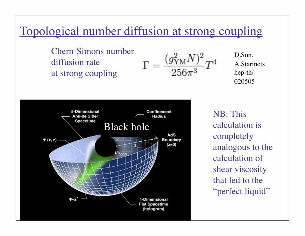
Black hole

D.Son, A.Starinetshep-th/020505

Topological number diffusion at strong couplingChern-Simons numberdiffusion rateat strong coupling

NB: This calculation is completely analogous to the calculation of shear viscosity that led to the “perfect liquid”

33

Classical topological solutions at strong coupling? yes: D-instantons in (dual) weakly coupled supergravity

D-instanton as an Einstein-Rosenwormhole;the flow of RR chargedown the throat of the wormhole describes change of chirality

D-instantons as a source of multiparticle production in N=4 SYM?DK, E.Levin, arXiv:0910.3355

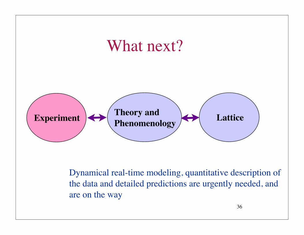
What next?

36

Experiment Theory andPhenomenology Lattice

Dynamical real-time modeling, quantitative description of the data and detailed predictions are urgently needed, and are on the way

37Supported by RIKEN-BNL, BNL-CATHIE, and Stony Brook University

Save the date: April 26-30, 2010

http://www.bnl.gov/riken/hdm/

P- and CP-odd effects in: nuclear, particle, condensed matter physics and cosmology

Organizing Committee

• Kenkji Fukushima (Kyoto Univ)

• Dmitri Kharzeev (BNL)

• Harmen Warringa (Johann Wolfgang Goethe-Univ)

• Abhay Deshpande (Stony Brook Univ. / RBRC)

• Sergei Voloshin (Wayne State Univ.)

International Advisory Committee

• J. Bjorken (SLAC)

• H. En'yo (RIKEN)

• M. Gyulassy (Columbia Univ.)

• F. Karsch (BNL & Bielefeld)

• T.D. Lee (Columbia Univ.)

• A. Nakamura (Hiroshima Univ.)

• M. Polikarpov (ITEP)

• K. Rajagopal (MIT)

• V. Rubakov (INR)

• J. Sandweiss (Yale Univ.)

• E. Shuryak (Stony Brook Univ.)

• A. Tsvelik (BNL)

• N. Xu (LBNL)

• V. Zakharov (ITEP)

38

Back-up slides

Further tests at RHIC

• Parity-odd observable?• Correlations for identified hadrons? ? • Low-energy run: the effect is expected to weaken below the deconfinement/chiral symmetry transition• P-odd decays? R. Millo & E.Shuryak, ‘09

• Double diffractive production in pp collisions: sphaleron decay in magnetic field?

KS0

40

Disentangleazimuthal,p_t dependencefrom the data:

A.Bzdak, V.Koch, J.Liao,arXiv:0912.5050

P-odd-correlated pairs are produced at small p_t!?

26th winter workshop on nuclear dynamics, ocho … · 1 the chiral magnetic effect and local parity...

Documents