General rights Copyright and moral rights for the publications made accessible in the public portal are retained by the authors and/or other copyright owners and it is a condition of accessing publications that users recognise and abide by the legal requirements associated with these rights.

Users may download and print one copy of any publication from the public portal for the purpose of private study or research.

You may not further distribute the material or use it for any profit-making activity or commercial gain

You may freely distribute the URL identifying the publication in the public portal If you believe that this document breaches copyright please contact us providing details, and we will remove access to the work immediately and investigate your claim.

Downloaded from orbit.dtu.dk on: Feb 24, 2020

275 Candidates and 149 Validated Planets Orbiting Bright Stars in K2 Campaigns 0–10

Mayo, Andrew W.; Vanderburg, Andrew; Latham, David W.; Bieryla, Allyson; Morton, Timothy D.;Buchhave, Lars A.; Dressing, Courtney D.; Beichman, Charles; Berlind, Perry; Calkins, Michael L.Published in:Astrophysical Journal

Link to article, DOI:10.3847/1538-3881/aaadff

Publication date:2018

Document VersionPublisher's PDF, also known as Version of record

Link back to DTU Orbit

Citation (APA):Mayo, A. W., Vanderburg, A., Latham, D. W., Bieryla, A., Morton, T. D., Buchhave, L. A., ... Winters, J. G.(2018). 275 Candidates and 149 Validated Planets Orbiting Bright Stars in

K2 Campaigns 0–10. Astrophysical

Journal, 155(3), [136]. https://doi.org/10.3847/1538-3881/aaadff

275 Candidates and 149 Validated Planets Orbiting Bright Stars in K2 Campaigns 0–10

Andrew W. Mayo1,2,3,20,21 , Andrew Vanderburg3,4,20,22 , David W. Latham3 , Allyson Bieryla3 , Timothy D. Morton5 ,Lars A. Buchhave1,2 , Courtney D. Dressing6,7,22 , Charles Beichman8, Perry Berlind3, Michael L. Calkins3 ,

David R. Ciardi8 , Ian J. M. Crossfield9, Gilbert A. Esquerdo3 , Mark E. Everett10 , Erica J. Gonzales11,20, Lea A. Hirsch6 ,Elliott P. Horch12 , Andrew W. Howard13 , Steve B. Howell14 , John Livingston15 , Rahul Patel16 , Erik A. Petigura13,23 ,Joshua E. Schlieder17, Nicholas J. Scott14 , Clea F. Schumer3, Evan Sinukoff13,18 , Johanna Teske19,24, and Jennifer G. Winters3

1 DTU Space, National Space Institute, Technical University of Denmark, Elektrovej 327, DK-2800 Lyngby, Denmark; awm@space.dtu.dk2 Centre for Star and Planet Formation, Natural History Museum of Denmark & Niels Bohr Institute, University of Copenhagen, Øster Voldgade 5-7, DK-1350

Copenhagen K., Denmark3 Harvard–Smithsonian Center for Astrophysics, 60 Garden Street, Cambridge, MA 02138, USA

4 Department of Astronomy, University of Texas at Austin, Austin, TX 76712, USA5 Department of Astrophysical Sciences, 4 Ivy Lane, Peyton Hall, Princeton University, Princeton, NJ 08544, USA

6 Astronomy Department, University of California, Berkeley, CA 94720, USA7 Division of Geological & Planetary Sciences, California Institute of Technology, 1200 East California Boulevard MC 150-21, Pasadena, CA 91125 USA

8 NASA Exoplanet Science Institute, California Institute of Technology, Pasadena, CA 91125, USA9 Department of Physics and Kavli Institute for Astrophysics and Space Research, Massachusetts Institute of Technology, Cambridge, MA 02139, USA

10 National Optical Astronomy Observatory, 950 North Cherry Avenue, Tucson, AZ 85719, USA11 Department of Astronomy and Astrophysics, University of California, Santa Cruz, CA 95064, USA

12 Department of Physics, Southern Connecticut State University, 501 Crescent Street, New Haven, CT 06515, USA13 Cahill Center for Astrophysics, California Institute of Technology, Pasadena, CA 91125, USA

14 Space Science and Astrobiology Division, NASA Ames Research Center, Moffett Field, CA 94035, USA15 Department of Astronomy, The University of Tokyo, 7-3-1 Hongo, Bunkyo-ku, Tokyo 113-0033, Japan16 Infrared Processing and Analysis Center, California Institute of Technology, Pasadena, CA 91125, USA

17 NASA Goddard Space Flight Center, Greenbelt, MD 20771, USA18 Institute for Astronomy, University of Hawai‘i at Mānoa, Honolulu, HI 96822, USA

19 Carnegie Observatories, 813 Santa Barbara Street, Pasadena, CA 91101, USAReceived 2017 December 15; revised 2018 January 18; accepted 2018 January 25; published 2018 March 6

Abstract

Since 2014, NASA’s K2 mission has observed large portions of the ecliptic plane in search of transiting planets andhas detected hundreds of planet candidates. With observations planned until at least early 2018, K2 will continue toidentify more planet candidates. We present here 275 planet candidates observed during Campaigns 0–10 of the K2mission that are orbiting stars brighter than 13 mag (in Kepler band) and for which we have obtained high-resolution spectra (R= 44,000). These candidates are analyzed using the vespa package in order to calculate theirfalse-positive probabilities (FPP). We find that 149 candidates are validated with an FPP lower than 0.1%, 39 ofwhich were previously only candidates and 56 of which were previously undetected. The processes of datareduction, candidate identification, and statistical validation are described, and the demographics of the candidatesand newly validated planets are explored. We show tentative evidence of a gap in the planet radius distribution ofour candidate sample. Comparing our sample to the Kepler candidate sample investigated by Fulton et al., weconclude that more planets are required to quantitatively confirm the gap with K2 candidates or validated planets.This work, in addition to increasing the population of validated K2 planets by nearly 50% and providing newtargets for follow-up observations, will also serve as a framework for validating candidates from upcoming K2campaigns and the Transiting Exoplanet Survey Satellite, expected to launch in 2018.

Key words: methods: data analysis – planets and satellites: detection – techniques: photometric

Supporting material: machine-readable tables

1. Introduction

The field of exoplanets is relatively young compared to mostother disciplines of astronomy: the announcement of the firstexoplanet orbiting a star similar to our own was made only in199525 (Mayor & Queloz 1995). Since then, the field has

expanded rapidly, with several thousand exoplanets havingnow been discovered. With many upcoming extremely largetelescopes, the number of known exoplanets and our under-standing of them will only increase.One of the most important moments in the history of exoplanet

science was the beginning of the Kepler mission (Boruckiet al. 2008). Launched in 2009, the Kepler space telescopeobserved over 100,000 stars in a single patch of sky for four yearsin order to look for transits. Kepler has been an overwhelmingsuccess. According to the NASA Exoplanet Archive26 (accessed2018 February 14), it is currently responsible for 2341 verifiedexoplanets, more than every other exoplanet survey combined.

The Astronomical Journal, 155:136 (25pp), 2018 March https://doi.org/10.3847/1538-3881/aaadff© 2018. The American Astronomical Society. All rights reserved.

20 National Science Foundation Graduate Research Fellow.21 Fulbright Fellow.22 NASA Sagan Fellow.23 NASA Hubble Fellow.24 Carnegie Origins Fellow, jointly appointed by Carnegie DTM & CarnegieObservatories.25 The exoplanet 51 Peg b was not fully confirmed to be a planet until theabsolute mass was measured by Martins et al. (2015). Moreover, a reportedbrown dwarf discovered in 1989 (Latham et al. 1989) may in fact be anexoplanet, depending on its inclination. 26 https://exoplanetarchive.ipac.caltech.edu/

1

Unfortunately, in 2013 the second of four reaction wheels onthe Kepler spacecraft failed, preventing the spacecraft fromlooking at its designated field and bringing an end to theoriginal mission. Fortunately, a follow-up mission, called K2,was developed that used the spacecraft’s thrusters as amakeshift third reaction wheel (Howell et al. 2014). Unlikethe original Kepler mission, the K2 mission must observe newfields roughly every 83 days.27 As a result, K2 observations aredivided into “campaigns”, each corresponding to a field.

With every new campaign, K2 observes more bright starsand finds more planets orbiting these stars, so there are newbright targets available for follow-up such as radial velocity(RV) measurements or transmission spectroscopy. K2 has ledto the discovery of numerous candidate and confirmed planets(Crossfield et al. 2015; Foreman-Mackey et al. 2015; Montetet al. 2015; Vanderburg et al. 2015b, 2016b; Adams et al. 2016;Barros et al. 2016; Crossfield et al. 2016; Schlieder et al.2016; Sinukoff et al. 2016; Pope et al. 2016; Dressinget al. 2017b; Hirano et al. 2017; Martinez et al. 2017), aswell as to the identification of planets orbiting rare types ofstars, including particularly bright nearby dwarf stars (Petiguraet al. 2015; Vanderburg et al. 2016a; Christiansen et al. 2017;Crossfield et al. 2017; Niraula et al. 2017; Rodriguezet al. 2017a, 2017b), young, pre-main-sequence stars (Mannet al. 2016; David et al. 2016), and disintegrating planetarymaterial transiting a white dwarf (Vanderburg et al. 2015a).

Here, we take advantage of the large number of bright starsobserved by K2 and present the identification and follow-up ofa sample of 275 exoplanet candidates orbiting stars (brighterthan 13 mag) in the Kepler bandpass identified from K2Campaigns 0 through 10. Since the beginning of the K2mission, we have also obtained spectra for all of our candidates,as well as many high-resolution imaging observations, in orderto measure the candidate host stars’ parameters and identifynearby stars (both types of follow-up aid in identification andruling out of false-positive scenarios). We also attempt tovalidate28 our candidates with vespa, a statistical validationtool developed by Morton (2012, 2015b), finding 149 to bevalidated with a false-positive probability (FPP) lower than0.1%. Of these newly validated exoplanets, 39 were previouslyonly exoplanet candidates and 56 have not been previouslydetected. This work will increase the validated K2 planetsample from 212 (according to the Mikulski Archive for SpaceTelescopes29; accessed 2018 February 14) to 307, an increase

of nearly 50%. Similarly, this work increases the K2 candidatesample by ∼20%.In this paper, we describe the identification and analysis of

our candidate sample, as well as our validation process and theresulting validated planet sample. Section 2 discusses theprocess by which we use K2 data to identify exoplanetcandidates. Section 3 describes our ground-based observationsof the planet candidate host stars detected by K2. Section 4explains the analysis of the K2 light curves and the follow-upspectroscopy and high-contrast imaging. Section 5 details howwe use vespa to calculate FPPs for our planet candidates.Section 6 presents the results of our candidate identification,vetting, follow-up observations, and analysis in detail for asingle, instructive planet. Then the results for the entire planetcandidate sample are similarly presented. In Section 7 wediscuss the results of our work, including confirmation offeatures in the exoplanet population previously identified usingdata from the original Kepler mission. Finally, we summarizeand conclude in Section 8.

2. Pixels to Planets

In this section, we first explain how K2 observations arecollected, then we describe the process by which systematicerrors are removed from K2 data, and finally we discuss theanalysis of the systematics-corrected K2 data in order toidentify planet candidates.

2.1. K2 Observations

Since 2014, the K2 mission has served as the successor to theoriginal Kepler mission. By observing fields along the eclipticplane and firing its thrusters approximately once every sixhours, the probe can maintain an unstable equilibrium againstsolar radiation. However, the spacecraft can only point towarda given field for roughly 83 days before re-pointing (in order tokeep sunlight on the spacecraft panels and out of its telescope).Because of on-board data storage constraints, not all data

collected by the CCD array can be retained and transmitted tothe ground. As a result, targets must be identified within eachcampaign field prior to observation so that non-target data canbe discarded and a postage stamp (a small group of pixels)around each target can be saved and transmitted to the ground.In the original Kepler mission, the primary objective was to

determine the frequency of Earth-like planets orbiting Sun-likestars (Batalha et al. 2010a). Although some planet searchtargets were selected during mission adjustments and otherswere selected through a Guest Observer (GO) program forsecondary science objectives, most targets were selected pre-launch for the primary objective. However, K2 operates in avery different manner. For each K2 campaign, targets areexclusively selected through the GO program, which evaluatesobserving proposals submitted by the astronomical communityfor any scientific objective, not just exoplanet-related objec-tives. Ideally, GO proposals have scientifically compellinggoals that can be achieved through K2 observations and cannoteasily be achieved with other instruments or facilities.In a typical K2 campaign, the number of targets ranges

between 10,000 and 40,000 with long-cadence observations(≈30-minute integration), and about 50–200 with short-cadence observations (≈1-minute integration). Exceptionsinclude C0, which served primarily as a proof-of-conceptcampaign to show that the K2 mission was viable, and C9,

27 Roughly 75 of those days are devoted to science.28 The difference between an exoplanet candidate and a validated exoplanet isvery important. During the original Kepler mission, an exoplanet candidate wasa transit signal that had passed a battery of astrophysical false-positive andinstrumental false-alarm tests. In K2, however, the usage is looser; the term iscommonly used to refer to any exoplanet signal that a particular team hasidentified as a possible planet. So long as the reasoning is sound and the resultsare published, the signal is effectively a candidate. A validated planet is acandidate that has been vetted with follow-up observations and determinedquantitatively to be far more likely an exoplanet than a false positive (accordingto some likelihood threshold). Validated planets, because confidence in theirplanethood is higher than for a regular candidate, are far more promising targetsthan planet candidates for follow-up observations, characterization, andeventual confirmation. We note that validation is not the same as confirmation,which is ideally attained through a reliable mass determination. In this work,we are in general not attempting to “confirm” planets. Confirmation is morerigorous than validation, in the same way that validation is more rigorous thancandidacy. Confirmation is usually accomplished via the RV method, the TTVmethod, or, less commonly, methods such as a full photodynamical modelingsolution (e.g., Carter et al. 2011) or Doppler tomography (e.g., Zhouet al. 2016).29 https://archive.stsci.edu/k2/published_planets/search.php

2

The Astronomical Journal, 155:136 (25pp), 2018 March Mayo et al.

which focused on microlensing targets in the Galactic Bulge.Both C0 and C9 had fewer targets than normal in both longcadence and short cadence. It should also be noted that thereare occasional overlaps between campaign fields. Despite fewernew targets, overlaps provide a longer baseline of observationsfor targets of interest in the overlapping region.

This paper focuses on Campaigns 0 through 10 (excludingCampaign 9). However, the process implemented in thisresearch can easily be extended and applied to additional K2campaigns.

2.2. K2 Data Reduction

Because of the loss of two reaction wheels, the Keplertelescope is perpetually drifting off target and must be regularlycorrected by thruster fires, causing shifts in the pixels thattargets fall on. These shifts, coupled with variable sensitivitybetween pixels on the telescope CCDs and variable amounts ofstarlight falling inside photometric apertures, lead to systematicvariations in the signal from K2 targets, introducing noise intothe photometric measurements. Howell et al. (2014) estimatedthat raw K2 precision is roughly a factor of 3–4 times worsethan the original Kepler precision (depending on stellarmagnitude). Fortunately, an understanding of the motion ofthe Kepler spacecraft allows for modeling and correction of theinduced systematic noise. In particular, we rely on the methodof systematic correction described by Vanderburg & Johnson(2014, hereafter referred to as VJ14), as well as the updates tothe method described in Vanderburg et al. (2016a, hereafterreferred to as V16). We briefly describe here the methoddeveloped by VJ14.

First, 20 different aperture masks were chosen for each targetstar, 10 circular masks of varying size and 10 masks shapedliked the Kepler pixel response function (PRF) for the targetwith varying sensitivity cutoffs. These masks were used toperform simple aperture photometry to produce 20 different“raw” light curves. Then the motion of the target star across theCCD was estimated by calculating centroid position for eachcadence.30 Next, the recurrent path of the centroid across theCCD between thruster fires was identified. Data collectedduring thruster fires were identified and removed. Then, foreach of the 20 raw light curves produced, low-frequencyvariations (>1.5 days) were removed with a basis spline, andthe relationship between centroid position and flux was fit witha piecewise function. Because the centroid path would shift ontimescales longer than 5–10 days, the flux-centroid piecewisefunction was applied separately to each light-curve segment of5–10 days. This function was then used to correct the raw dataso that low-frequency variations could be recalculated. Thisprocess was then repeated iteratively until convergence.Finally, after all 20 raw light curves per star were processedin this way, a “best” aperture was chosen to maximizephotometric precision. An example of a light curve before andafter the full data reduction procedure can be seen in Figure 1for the planet host EPIC 212521166. We note that light fromany nearby companion star could potentially enter the bestaperture mask, which may lead to a diluted transit and anunderestimated planet radius (Ciardi et al. 2015; Hirsch

et al. 2017). However, we expected this effect to be smalleven when present and therefore did not correct for it.

2.3. Identifying Threshold-crossing Events

After the roll systematics were removed from the photometryaccording to the method described by VJ14, we conducted atransit search of each K2 target using the method ofVanderburg et al. (2016b). We give a short description of thetransit search process here.First, low-frequency variations were removed via a basis

spline and outliers were removed. Then a box-least-squares(BLS) periodogram (Kovács et al. 2002) was calculated overperiods between 2.4 hr and half the length of the campaign. Allperiodic decreases in brightness with a signal-to-noise ratio(S/N)>9 were investigated. If putative transits lasted longerthan 20% of their period, were composed of a single data point,or changed depth by over 50% when the lowest point wasremoved, the signal was removed and the BLS periodogramrecalculated. Any detection passing these tests was deemed athreshold-crossing event (TCE). We identified ∼30,000 TCEsacross C0–C10 in this manner.Each TCE was fit with the Mandel & Agol (2002) transit

model to estimate transit parameters, then the TCE wasremoved from the light curve, and the BLS periodogram wasrecalculated. After all TCEs had been identified, theysubsequently underwent “triage,” in which each candidatewas inspected by eye in order to remove obvious astrophysicalfalse positives and instrumental false alarms from subsequentanalysis. TCEs identified as neither type of false signal passedthe triage phase and moved on to a “vetting” phase.

2.4. Identifying K2 Candidates

During vetting, we subjected the surviving TCEs to a batteryof additional tests to identify astrophysical false positives andinstrumental false alarms. Some of these tests were identical orsimilar to the tests conducted for the Kepler mission, whileothers are specific to K2 data. For each test we produced a

Figure 1. Example of the K2 systematics reduction process on the light curveof the planet host EPIC 212521166. The blue points show the light curvebefore correcting for the systematics induced by the roll motion of the Keplerspacecraft, while the yellow points show the same light curve after thosesystematics have been removed via the data reduction process summarized inSection 2.2 and documented in Vanderburg & Johnson (2014) and Vanderburget al. (2016b). The remaining downward dips in the corrected (yellow) lightcurve are transits of a mini-Neptune sized exoplanet, validated in this work andpreviously confirmed in Osborn et al. (2017).

30 Although it is possible to produce light curves by decorrelating withcentroid positions measured from each star, we used the centroids measuredfrom one hand-selected isolated, bright K2 target per campaign, which wefound gives better results.

3

The Astronomical Journal, 155:136 (25pp), 2018 March Mayo et al.

diagnostic plot, examples of which are shown in Figures 2–4.Here we describe the tests we conducted in more detail.

1. The times of the in-transit points of a TCE werecompared against the position of the Kepler spacecraftat these times, as many instrumental false alarms werecomposed of data points near the edges of Kepler rollswhere the K2 flat field is less well constrained, and ouranalysis method can leave in systematics. The plots weused to identify these false alarms are shown in Figures 2and 3.

2. We compared the signal of a TCE in light curvesproduced using multiple different photometric apertures.This test is a powerful way to identify signals caused byinstrumental systematics (as these systematics presentdifferently in different photometric apertures), as well as

identifying astrophysical false positives, such as when acandidate transit signal was due to contamination from anearby star. An example of these tests is shown inFigure 3. We note that although this test rules out transitsor eclipses originating from a nearby companion, it doesnot rule out the possibility of light contamination from anearby companion, which could dilute the observedtransit and lead to an underestimation of the planetaryradius (Ciardi et al. 2015; Hirsch et al. 2017).

3. Individual transits of a TCE were visually inspected,since instrumental false alarms were less likely to haveconsistent, planet-like transit depths or shapes (seeFigure 2). This metric is qualitatively similar to the“transit patrol” metrics introduced in the DR25 Keplerplanet candidate catalog (in particular the Rubble,

Figure 2. Diagnostic plots for EPIC 212521166.01. Left column, first (top) and second rows: K2 light curves without and with low-frequency variations removed,respectively. The low-frequency variations alone are modeled in red in the first row, whereas the best-fit transit model is shown in red in the second row. Verticalbrown dotted lines denote the regions into which the light curve was separated to correct roll systematics. Left column, third and fourth rows: phase-folded, low-frequency corrected K2 light curves. In the third row, the full light curve is shown (points more than one half-period from the transit are gray), whereas in the fourthrow, only the light curve near transit is shown. The red line is the best-fit model, and the blue points are binned data points. Middle column, first and second rows:arclength of centroid position of star vs. brightness, after and before roll systematics correction, respectively. Red points denote in-transit data. In the second row,small orange points denote the roll systematics correction made to the data. Middle column, third row: separate plotting and modeling of odd (left panel) and even(right panel) transits, with orange and blue data points, respectively. The black line is the best-fit model, the horizontal red line denotes the modeled transit depth, andthe vertical red line denotes the mid-transit time (this is useful for detecting binary stars with primary and secondary eclipses). Middle column, fourth row: light curvedata in and around the expected secondary eclipse time (for zero eccentricity). Blue data points are binned data, the horizontal red line denotes a relative flux=1, andthe two vertical red lines denote the expected beginning and end of the secondary eclipse. Right column: individual transits (vertically shifted from one another) withthe best-fit model in red and the vertical blue lines denoting the beginning and end of transit.

4

The Astronomical Journal, 155:136 (25pp), 2018 March Mayo et al.

Marshall, Chases, and Zuma tests; Thompson et al.2017).

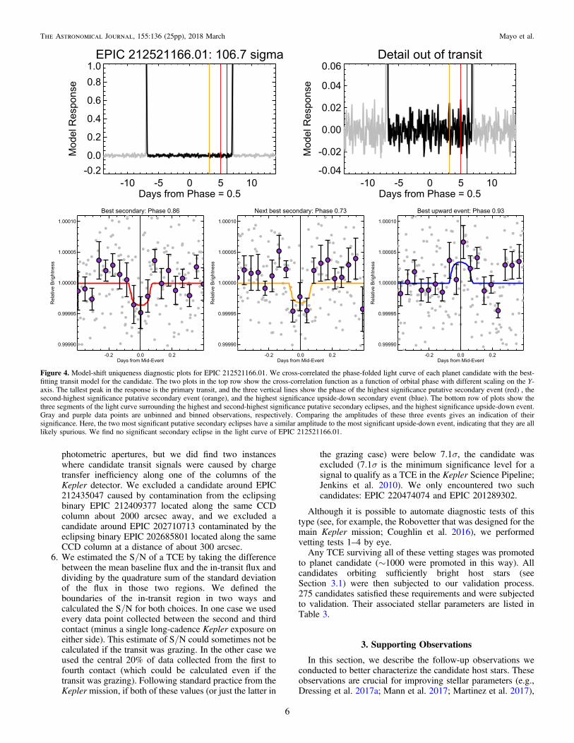
4. Flux-centroid motion, phase variations (possibly causedby relativistic beaming, reflected light, or ellipsoidaleffects), differences in depth between odd- and even-numbered transits, and secondary eclipses were allsearched for as evidence of astrophysical false positives.Similar tests have been used since the beginning of theKepler mission (Batalha et al. 2010b). Example diag-nostic plots for identifying phase variations, the differ-ence between even- and odd-numbered transits, andsecondary eclipses near phase 0.5 are shown in Figure 2;flux-centroid shift tests are shown in Figure 3. Wesearched for secondary eclipses at arbitrary phases (notnecessarily near phase=0.5) using the model-shiftuniqueness test designed by Coughlin et al. (2016). We

show diagnostic plots for the model-shift uniqueness testin Figure 4.

5. We searched for astrophysical false-positive scenarios byephemeris matching. Sometimes the pixels surrounding atarget star can be contaminated with a small amount oflight from other nearby stars. When those nearby stars arevariable themselves (like eclipsing binaries), the varia-bility from the nearby stars can be introduced into thetarget’s light curve (Coughlin et al. 2014). We identifiedcases where this happened by searching for planetcandidates that have the same period (or integer multiplesof the same period) and time of transit as eclipsingbinaries observed by K2 using the same criteria asCoughlin et al. (2014). We found no examples ofmatched ephemerides due to direct PRF overlap that wehad not also identified in our tests with multiple

Figure 3. Diagnostic plots for EPIC 212521166.01. Left column, first (top), second, and third rows: images from the first Digital Sky Survey, the second Digital SkySurvey, and K2, respectively, each with a scale bar near the top and an identical red polygon to show the shape of the photometric aperture chosen for reduction. TheK2 image is rotated into the same orientation as the two archival images (north is up). Middle column, top row: multiple panels of uncorrected brightness vs. arclength,chronologically ordered and separated into the divisions in which the roll systematics correction was calculated. In-transit data points are shown in red, orange pointsdenote the brightness correction applied to remove systematics. Middle column, bottom row: variations in the centroid position of the K2 image. In-transit points arered. The discrepancy (in standard deviations) between the mean centroid position in transit and out-of-transit is shown on the right side of the plot. Right column, firstrow: the K2 light curve near transit as calculated using three differently sized apertures: small mask (top panel), medium mask (middle panel), and large mask (bottompanel), each with the identical best-fit model in red. Aperture-size dependent discrepancies in depth could suggest background contamination from another star. Rightcolumn, third row: the K2 image overlaid with the three masks from the previous plot shown (in this figure, the large mask is fully outside the postage stamp and istherefore not visible).

5

The Astronomical Journal, 155:136 (25pp), 2018 March Mayo et al.

photometric apertures, but we did find two instanceswhere candidate transit signals were caused by chargetransfer inefficiency along one of the columns of theKepler detector. We excluded a candidate around EPIC212435047 caused by contamination from the eclipsingbinary EPIC 212409377 located along the same CCDcolumn about 2000 arcsec away, and we excluded acandidate around EPIC 202710713 contaminated by theeclipsing binary EPIC 202685801 located along the sameCCD column at a distance of about 300 arcsec.

6. We estimated the S/N of a TCE by taking the differencebetween the mean baseline flux and the in-transit flux anddividing by the quadrature sum of the standard deviationof the flux in those two regions. We defined theboundaries of the in-transit region in two ways andcalculated the S/N for both choices. In one case we usedevery data point collected between the second and thirdcontact (minus a single long-cadence Kepler exposure oneither side). This estimate of S/N could sometimes not becalculated if the transit was grazing. In the other case weused the central 20% of data collected from the first tofourth contact (which could be calculated even if thetransit was grazing). Following standard practice from theKepler mission, if both of these values (or just the latter in

the grazing case) were below 7.1σ, the candidate wasexcluded (7.1σ is the minimum significance level for asignal to qualify as a TCE in the Kepler Science Pipeline;Jenkins et al. 2010). We only encountered two suchcandidates: EPIC 220474074 and EPIC 201289302.

Although it is possible to automate diagnostic tests of thistype (see, for example, the Robovetter that was designed for themain Kepler mission; Coughlin et al. 2016), we performedvetting tests 1–4 by eye.Any TCE surviving all of these vetting stages was promoted

to planet candidate (∼1000 were promoted in this way). Allcandidates orbiting sufficiently bright host stars (seeSection 3.1) were then subjected to our validation process.275 candidates satisfied these requirements and were subjectedto validation. Their associated stellar parameters are listed inTable 3.

3. Supporting Observations

In this section, we describe the follow-up observations weconducted to better characterize the candidate host stars. Theseobservations are crucial for improving stellar parameters (e.g.,Dressing et al. 2017a; Mann et al. 2017; Martinez et al. 2017),

Figure 4. Model-shift uniqueness diagnostic plots for EPIC 212521166.01. We cross-correlated the phase-folded light curve of each planet candidate with the best-fitting transit model for the candidate. The two plots in the top row show the cross-correlation function as a function of orbital phase with different scaling on the Y-axis. The tallest peak in the response is the primary transit, and the three vertical lines show the phase of the highest significance putative secondary event (red) , thesecond-highest significance putative secondary event (orange), and the highest significance upside-down secondary event (blue). The bottom row of plots show thethree segments of the light curve surrounding the highest and second-highest significance putative secondary eclipses, and the highest significance upside-down event.Gray and purple data points are unbinned and binned observations, respectively. Comparing the amplitudes of these three events gives an indication of theirsignificance. Here, the two most significant putative secondary eclipses have a similar amplitude to the most significant upside-down event, indicating that they are alllikely spurious. We find no significant secondary eclipse in the light curve of EPIC 212521166.01.

6

The Astronomical Journal, 155:136 (25pp), 2018 March Mayo et al.

which in turn can help differentiate between a transiting planetand various false-positive scenarios (i.e., stellar binary config-urations) that might prefer different regions of stellar parameterspace. We first discuss high-resolution optical spectroscopy ofthe planet candidate host stars from the Tillinghast ReflectorEchelle Spectrograph (TRES), followed by speckle imagingfrom the Differential Speckle Survey Instrument (DSSI) andthe NASA Exoplanet Star and Speckle Imager (NESSI) at theWIYN telescope,31 the Gemini South telescope, and theGemini North telescope, and finally, adaptive optics (AO)imaging from Keck Observatory, Palomar Observatory,Gemini South Observatory, Gemini North Observatory, andthe Large Binocular Telescope Observatory.

3.1. TRES Observations

All of the spectra used in this work were obtained with TRES,a spectrograph with a resolving power of R=44,000 and one oftwo spectrographs for the 1.5 m Tillinghast telescope at theWhipple Observatory on Mt. Hopkins in Arizona. We obtainedat least one usable TRES spectrum of each of the planetcandidate host stars that we consider in this work and that wesubject to our validation process (see Section 4.2 for ourdefinition of “usable”). With a few exceptions, we only observedcandidates brighter than 13 mag in the Kepler band with TRESbecause of the lengthy integration time required to collectspectra of stars fainter than this and the difficulty of subsequentfollow-up observations (for example, with precise radialvelocities) at other facilities. This limitation reduced the numberof candidates we considered for validation significantly, from∼1000 to 275. In the future, observing these fainter candidates,either with TRES or other spectrographs on larger telescopes,could potentially more than double the number of K2 planets forour analysis.

3.2. Speckle Observations

We observed many of our planet candidates with speckleimaging from either the 3.5m WIYN telescope, the Gemini-South 8.1m telescope, or the Gemini-North 8.1m telescope.Together, the three telescopes collected 162 speckle images of73 stars with DSSI (Horch et al. 2009). DSSI is a speckle-imaging instrument that travels between different telescopes.For each of the 73 targets, we collected DSSI speckle images atnarrowband filters centered at 6920 and 8800Å (at least one ofeach for every target). These observations were made in 2015September and October, as well as in 2016 January, April,and June.

Furthermore, 160 speckle images were collected for adistinct sample of 70 stars at the WIYN telescope usingNESSI, which is essentially a newer version of the DSSIinstrument. For each of the 70 targets, we collected NESSIspeckle images at narrowband filters centered at 5620 and8320Å (at least one of each). These observations were made in2016 October through November and 2017 March throughMay. A list of the observed stars can be found in Table 1.

3.3. AO Observations

In addition to speckle imaging, we also observed many ofour planet candidate host stars with AO imaging.We collected 47 AO images for 45 stars on the Keck II 10m

telescope in K filter with the Near Infra Red Camera 2(NIRC2); 5 of these stars were also imaged using NIRC2 inJ band. All of these observations were made during 2015 April,July, August, and October and in 2016 January and February.We collected 27 AO images for 27 stars on the Palomar

5.1m Hale telescope in K filter with the Palomar High AngularResolution Observer (PHARO, Hayward et al. 2001); 6 ofthese stars were also imaged using PHARO in J band. All ofthese observations were made during 2015 February, May, andAugust and in 2016 June, September, and October.We collected 19 AO images for 18 stars on the Gemini-

North 8.1m telescope in K band with the Near InfraRedImager and spectrograph (NIRI, Hodapp et al. 2003). Theseobservations were made during 2015 October and Novemberand in 2016 June and October.We collected a single AO image on the Large Binocular

Telescope in K filter with the L/M-band mid-infraRed Camera(LMIRCam, Leisenring et al. 2012). This observation wasmade in 2015 January.There was some overlap between instruments; overall, AO

images were collected for a total of 80 systems. A list of theobserved stars can be found in Table 1.

4. Data Analysis

After all of the photometry had been reduced and all of thenecessary follow-up observations had been collected, the nextstep was to analyze the data, calculate relevant parameters, andprepare the results for the validation process. In this section, weexplain the process of fitting a model to our reduced lightcurves (to determine transit parameters and create folded lightcurves), analyzing our spectra (to calculate stellar parameters),and extracting and reducing data from our high-contrast images(to create contrast curves).

4.1. K2 Light Curves

4.1.1. Simultaneous Fitting of K2 Systematics and Transit Parameters

In Sections 2.2, 2.3, and 2.4, we described the process ofcorrecting K2 photometry for instrumental systematics andexploring the reduced light curves for candidates. After thesesteps were completed, the planet candidates needed to be morethoroughly characterized. In order to assess transit and orbitalparameters, we reproduced the K2 light curves for these planetcandidates by rederiving the systematics correction whilesimultaneously modeling the transits in the light curve. As inour original systematics correction, the light curve was divided

Table 1High-resolution Imaging

EPIC Filter Instrument

201110617 562 NESSI201110617 832 NESSI201111557 562 NESSI

(This table is available in its entirety in machine-readable form.)

31 The WIYN Observatory is a joint facility of the University of Wisconsin-Madison, Indiana University, the National Optical Astronomy Observatory,and the University of Missouri.

7

The Astronomical Journal, 155:136 (25pp), 2018 March Mayo et al.

into multiple sections and the systematics correction wasapplied to each section separately. A piecewise linear functionwas fit with breaks roughly every 0.25 arcsec (varying slightlyby target) to the arclength versus brightness relationshipdescribed in Section 2.2 (arclength is a one-dimensionalmeasure of position along the path an image centroid tracesout on the Kepler CCD camera). The low-frequency variationsin the light curve were modeled with a cubic spline (withbreakpoints every 0.75 days), and the transits themselves weremodeled with the Mandel & Agol (2002) transit model. The fitwas performed using a Levenberg–Marquardt optimization(Markwardt 2009), and all of the parameters from theoptimization (besides the transit parameters) were used inorder to correct the systematics of the light curve (once again)and remove the low-frequency variations (once again). Sincethese parameters were determined in a simultaneous fit with thetransits, the quality of the resulting light-curve reduction tendedto be better than that of the original light curves.

4.1.2. Final Estimation of Transit Parameters and Uncertainties

After we produced the systematics-corrected, low-frequency-extracted light curves, we analyzed them further in order toestimate final transit parameter values and their uncertainties.We based our model on the BATMAN Python package(Kreidberg 2015), which we used to calculate our synthetictransit light curves. We fit the transit light curves of all planetcandidates around a given star simultaneously so that over-lapping transits could be modeled, assuming that each of theplanets were non-interacting and on circular orbits. For eachplanet candidate, five parameters were included: the epoch (i.e.,time of first transit), the period, the inclination, the ratio ofplanetary to stellar radius (Rp/R*), and the semimajor axisnormalized to the stellar radius (a/R*). Additionally, twoparameters for a quadratic limb-darkening law were included(Kipping 2013), as well as a parameter to allow the baseline tovary (in case there was an erroneous systematic offset fromflux=1 outside of transit), and a noise parameter that assignedthe same uncertainties to each flux measurement (since fluxerror bars were not calculated in the K2 data reduction process).For all of these planet and system parameters we assumed auniform prior, except for the Rp/R* parameter for each planet,which we gave a log-uniform prior.

For each candidate system, the transit parameters in thismodel were estimated using emcee (Foreman-Mackey et al.2013), a Python package that runs simulations using a Markovchain Monte Carlo (MCMC) algorithm with an affine-invariantensemble sampler (Goodman & Weare 2010). In eachsimulation, the parameter space for a system with n candidateswas sampled with 8+10n chains (equal to twice the numberof model parameters). The MCMC process was run for either10,000 steps or until convergence, whichever came last.Convergence was defined according to the scale-reductionfactor (Gelman & Rubin 1992), a diagnostic that comparesvariance for individual chains against variance of the wholeensemble. A simulation was considered converged when thescale-reduction factor was less than 1.1 for each parameter. TheGelman–Rubin scale-reduction factor is properly defined forchains from distinct, non-communicating MCMC processes;however, we found that our simulations visually convergedmany times more quickly than the Gelman–Rubin diagnostic,so we decided the diagnostic would be sufficient for our

purposes. An example of a converged model fit against transitdata can be seen in Figure 5.Additionally, each simulation was checked after the mini-

mum number of steps (10,000) and at the end of the simulationfor any chains in the ensemble that could be easily categorizedas “bad,” i.e., trapped in a minimum of parameter space with apoorer best fit than the minimum of the ensemble majority. Indetail, a chain was classified as “bad” if both of the followingapplied:

1. The Kolmogorov–Smirnov statistic between the chainwith the highest likelihood step and the chain in questionwas greater than 0.5.

2. n1 100l gq q < ( ), where θl is the local maximumlikelihood (the maximum likelihood within the chain inquestion), θg is the global maximum likelihood through-out the ensemble, and n is the total number of steps. Thistest is our own invention, which is more likely to classifya chain as bad when its maximum likelihood is fartherfrom the global maximum likelihood. This test alsoaccounts for the length of the simulation, since themaximum likelihood within each chain should be closerto the global maximum likelihood for longer simulations.We include a factor of 100 in the denominator to makethe test sufficiently conservative, such that it only findsbad chains very rarely and only those extremely unlikelyto rejoin the ensemble in the lifetime of the simulation.

If a chain was deemed bad after 10,000 steps, its position inparameter space was updated to that of a good chain from theprevious step of the simulation. If a chain was deemed bad atthe end of the simulation, it was simply removed and notreplaced. Both after 10,000 steps and at the end of thesimulation, bad chains only occurred about 15% of the time,typically for only one or two chains in the ensemble.Transit fit parameters for all 275 candidates are listed in

Table 2 (along with some stellar parameters and validationresults). A representative sample of the converged posteriorsfor each exoplanet system transit fit has been archivedat10.5281/zenodo.1164791.

Figure 5. Fit of our transit model to corrected and normalized light curve datafor EPIC 212521166.01. The yellow points are the observed data, normalizedand phase-folded to the orbital period of the planet. The black line is our transitmodel with the median parameter values determined from an MCMC process.The dark blue and light blue regions are 1σ and 3σ confidence intervals,respectively.

8

The Astronomical Journal, 155:136 (25pp), 2018 March Mayo et al.

Table 2Planet Candidate Parameters

K2 Name EPIC T0 (BJD-2454833) P (days) a/R* i (deg) Rp/R* Rp (R⊕) R* (Re) M* (Me) Kp FPP Disposition Notes

K2-156 b 201110617.01 2750.1409±0.0028 0.813149 0.0000490.000050

-+ 4.4 1.1

0.7-+ 84.0 7.6

4.3-+ 0.0170 0.0011

0.0014-+ 1.14 0.08

0.10-+ 0.616 0.016

0.019-+ 0.642 0.019

0.022-+ 12.947 e1.00 04< - Planet L

201111557.01 2750.1621±0.0021 2.30237 0.000100.00011

-+ 12.6 8.0

2.8-+ 87.4 9.5

1.9-+ 0.0169 0.0015

0.0067-+ 1.31 0.12

0.52-+ 0.711 0.020

0.019-+ 0.746±0.023 11.363 e1.22 03- Candidate L

201127519.01 2752.5513 0.00120.0011

-+ 6.17837 0.00017

0.00019-+ 17.3 2.0

1.1-+ 88.8 1.0

0.8-+ 0.1151 0.0034

0.0049-+ 9.91 0.36

0.53-+ 0.789 0.017

0.025-+ 0.857 0.023

0.021-+ 11.558 L Candidate c

Notes.a Unless there is a deep secondary eclipse or ellipsoidal variations in the light curve, vespa cannot distinguish between a planet-sized star and a planet. In this case, Rp>8R⊕ and RV measurements cannot rule out theforeground eclipsing binary scenario. Therefore, no FPP value is reported.b Companion in aperture, therefore no FPP is reported.c AO/Speckle companion, therefore no FPP is reported.d Composite spectrum, therefore no FPP is reported.e Large RV amplitude variations confirm a binary in the system, therefore no FPP is reported.f vespa failed to find an FPP.

(This table is available in its entirety in machine-readable form.)

9

TheAstro

nomica

lJourn

al,

155:136(25pp),

2018March

Mayo

etal.

4.2. TRES Spectroscopy

We first visually inspected each of the spectra collected withTRES for our candidate host stars. Our main goal in visuallyinspecting the spectra was to identify cases in which the spectrawere composite or otherwise indicative of multiple stars in thesystem. We looked at diagnostic plots produced by the TRESpipeline, which showed various echelle orders and a cross-correlation between a synthetic template spectrum and a singlespectral order around 5280Å.

After identifying composite spectra and confirming that theothers were apparently single-lined, we prepared the spectrabefore determining the host stars’ parameters. In particular, wemanually removed cosmic rays from the spectra that might biasor otherwise affect the spectroscopic parameters we measured.We focused on three echelle orders in particular, orders 22, 23,and 24 (covering 5059–5158, 5135–5236, and 5214–5317Å,respectively), which are within the range we used to measurespectroscopic parameters.

After we visually inspected each spectrum and removingcosmic rays, we analyzed each TRES spectrum using theStellar Parameter Classification (SPC) tool, developed byBuchhave et al. (2012). SPC determines key stellar parametersthrough a comparison of the input spectrum (between 5050 and5360Å) to a library grid of synthetic model spectra, developedby Kurucz (1992). The library is four-dimensional, varying ineffective temperature Teff, surface gravity logg, metallicity[m/H], and line broadening (a good proxy for projectedrotational velocity, or vsini). [m/H] is estimated rather than[Fe/H] because all metallic absorption features are used todetermine metallicity rather than just iron lines. (SPC assumesthat all relative metal abundances are the same as in the Sun,and [m/H] simply scales all solar abundances by the samefactor.) This library grid spans Teff from 3500 K to 9750 K in250 K increments, logg from 0.0 to 5.0 (cgs) in 0.5 increments,[m/H] from −2.5 to +0.5 in 0.5 dex increments, and linebroadening from 0 km s−1 to 200 km s−1 in progressivelyspaced increments (from 1 km s−1 up to 20 km s−1). In total,the library contains 51,359 synthetic spectra. The stellarparameters derived using SPC can be found in Table 3.

We also calibrated TRES against Duncan et al. (1991) for theSHK stellar activity index, a measure of the strength of emissionin the cores of the H and K Ca II spectral absorption features.Our calibration was only performed over a range of0.244<B−V<1.629, 0.055<SHK<2.070, and vsini<20 km s−1. Additionally, we required a photon count of morethan 250,000 in the R and V continuum regions(3901.07± 10Å and 4001.07± 10Å, respectively). Withinthese ranges, we were able to calculate SHK for 28 of our

spectra collected for four stars. Although there are relativelyfew K2 planet candidates bright enough for this measurementon a 1 m telescope, it will be much more common withTransiting Exoplanet Survey Satellite (TESS). A note has beenmade for the relevant stars in Table 3 and the full results arelisted in Table 4. There is also a detailed description of the SHKcalibration process for TRES in the Appendix.In cases where we observed a candidate host star more than

once with TRES, we attempted to identify or rule out largevelocity variations indicating a stellar companion to the hoststar. (For this purpose we collected one new TRES spectrumeach for EPIC 220250254 and EPIC 210965800, but otherwiseexclusively used the spectra from which we derived stellarparameters.) We phased the radial velocities to the photometricephemeris and fit a sinusoid to the velocities at the period andephemeris of each candidate (and assuming a circular orbit) inorder to estimate the companion mass and mass uncertainty. Ifthe companion mass was more than 3σlower than 13 Jupitermasses, we ruled out the eclipsing binary scenario (seeSection 5.1). If the semi-amplitude of the companion masswas more than 1 km s−1, we labeled the system as a binary.Five systems were labeled binaries in this manner. If neither ofthe above cases was true, no action was taken.Out of the 233 candidate host stars, 43 had more than one

TRES spectrum available. The stellar parameters calculated forthe spectra of such candidates were combined via a weightedaverage based on the peak height of the cross-correlationfunction. The scatter between multiple spectra for the samecandidate was not large relative to the assumed systematicerrors. For example, Buchhave et al. (2012) set an internal errorfloor of 50 K for effective temperature; we found an averagestandard deviation of 40 K between spectra of the samecandidate, and the scatter was less 100 K for ∼90% ofcandidates with multiple spectra.There were some instances in which a TRES spectrum was

not considered good enough for stellar parameter estimationwith SPC. In particular, we did not use any spectrum for whichthe S/N per resolution element was <20 or the cross-correlation function peak height of the spectrum was <0.8.Furthermore, we did not use any spectra that yielded SPCresults outside of certain trustworthy ranges. Specifically, weonly used spectra that yielded 4250<Teff<6500 and linebroadening <50 km s−1. It should also be noted that all spectraused to determine stellar parameters were collected with TRESon or before 2017 June 10 (although some usable spectra havesince been collected, they were not retroactively included inour stellar parameter analysis). No planet candidate underwentthe validation process unless their host star had at least onespectrum (collected with TRES) that satisfied these criteria.

Table 3Stellar Parameters

EPIC Teff [m/H] log g R* (Re) M* (Me) Kp Notes

201110617 4460.0±50.0 −0.33±0.08 4.68±0.1 0.616 0.0160.019

-+ 0.642 0.019

0.022-+ 12.947 L

201111557 4720.0±50.0 −0.06±0.08 4.5±0.1 0.711 0.0200.019

-+ 0.746±0.023 11.363 L

201127519 5015.0±50.0 0.24±0.08 4.67±0.1 0.789 0.0170.025

-+ 0.857 0.023

0.021-+ 11.558 L

Notes.a Stellar parameters for this star are derived from a single spectrum with a cross-correlation function peak height <0.9 (but >0.8). We have decided that the resultingstellar parameters are trustworthy for this analysis, but provide a note for the reader’s discretion.b SHK values have been determined for this star and can be found in Table 4.

(This table is available in its entirety in machine-readable form.)

10

The Astronomical Journal, 155:136 (25pp), 2018 March Mayo et al.

4.3. Contrast Curves

We quantified the constraints placed on the presence ofadditional companions in our high-resolution (speckle and AO)imaging by calculating contrast curves. A contrast curvespecifies at a given distance from the target star how bright acompanion star would have to be in order to be detected.

After the speckle observations were collected, the data werereduced according to the method described in Furlan et al.(2017), yielding a high-contrast image of a candidate. Thenlocal minima and maxima were analyzed relative to the star’speak brightness to determine Δm (average sensitivity) and itsuncertainties within bins of radial distance from the target star.The contrast curves used in this research were the 5σupperlimit on Δm as a function of radial distance. A more detaileddescription of the data reduction process can be found inHowell et al. (2011). An example of a contrast curve can beseen in Figure 6.

As for AO observations, the creation of correspondingcontrast curves was performed by injecting fake sources intothe images and varying their brightness in order to determinethe brightness threshold for the detection algorithm being used.This process is described in greater detail in Crossfield et al.(2016) and Ziegler et al. (2017).

Note that these processes of creating a contrast curve werethe same regardless of wavelength. So in the instances thatmultiple speckle or AO images at different wavelengths wereavailable, multiple contrast curves were created that were allused in the validation process for a given candidate.

5. False-positive Probability (FPP) Analysis

5.1. The Application of vespa to Planet Candidates

Our validation work relied primarily on a method calledvalidation of exoplanet signals using a probabilistic algorithm,or vespa, a public package (Morton 2015b) based on the workof Morton (2012). It operates within a Bayesian framework andcalculates the FPP, the probability that a candidate is anastrophysical false positive rather than a true positive (i.e., aplanet).After photometry, spectroscopy, and any available high-

contrast imaging had been collected and reduced for acandidate system, that system underwent our validationprocedure using vespa. For each candidate, the followinginformation was supplied:

1. A folded light curve containing the planetary transit androughly one transit duration of baseline on either side.Identical error bars were assigned to all data points basedon the noise parameter determined by our transit-fittingprocedure. From this light curve, other planets in thesystem were removed using the best-fit parametersdetermined by the fitting procedure.

2. A secondary threshold limit. We calculated this limit byfirst cutting out all transits from all candidates in asystem. Then, for a given candidate, we phase-folded thedata to the candidate’s period, binned the baseline fluxaccording to the transit duration of the candidate,calculated the standard deviation between the binaverages, and multiplied by three. Effectively, we assertthat a secondary eclipse has not been detected at a 3σlevel or higher.

3. A contrast curve. When available, this lowered the FPPby eliminating the possibility of bound or backgroundstars above a certain brightness at a given projecteddistance, thus reducing the parameter space in which afalse-positive scenario could exist. Note that vespa does

Table 4Stellar SHK Activity Index

EPIC Date SHK

201437844 2017 Jan 08 0.1666 0.00310.0030

-+

201437844 2017 Mar 09 0.1698±0.0032201437844 2017 Mar 09 0.1589±0.0031201437844 2017 Mar 09 0.1712±0.0031201437844 2017 Mar 09 0.1651 0.0029

0.0030-+

201437844 2017 Mar 09 0.1624±0.0030201437844 2017 Mar 09 0.1633 0.0029

0.0030-+

201437844 2017 Mar 09 0.1614±0.0029201437844 2017 Mar 09 0.1692±0.0029201437844 2017 Mar 09 0.1622 0.0029

0.0030-+

201437844 2017 Mar 09 0.1635±0.0028201437844 2017 Mar 09 0.1593 0.0027

0.0029-+

201437844 2017 Mar 09 0.1615 0.00290.0028

-+

201437844 2017 Mar 09 0.1680 0.00290.0028

-+

201437844 2017 Mar 09 0.1646±0.0029201437844 2017 Mar 09 0.1639±0.0028201437844 2017 Mar 09 0.1651±0.0028201437844 2017 Mar 09 0.1656±0.0029201437844 2017 Mar 09 0.1693±0.0029201437844 2017 Mar 09 0.1641±0.0029201437844 2017 Mar 09 0.1680±0.0029205904628 2015 Jul 24 0.1550 0.0030

0.0029-+

205904628 2015 Sep 06 0.1453 0.00330.0031

-+

211424769 2015 Dec 09 0.3255 0.00390.0040

-+

211424769 2016 Jan 01 0.3144 0.00390.0040

-+

211993818 2015 Nov 27 0.4189 0.00450.0044

-+

211993818 2016 Feb 29 0.3851 0.00300.0031

-+

211993818 2016 Mar 02 0.3115 0.00280.0027

-+

Figure 6. Contrast curve developed from a speckle image at 692 nm (6920 Å)for candidate system EPIC 212521166. The contrast curve is plotted as Δm(average sensitivity to a companion in magnitude difference between theprimary and secondary) vs. angular separation (in arcseconds). Plus signs andcircles are maxima and minima, respectively, of the background sensitivity inthe image. The blue squares are the 5σ sensitivity limit within adjacent angularseparation annuli. The red line is the contrast curve itself, a spline fit to thesensitivity limit (the blue squares).

11

The Astronomical Journal, 155:136 (25pp), 2018 March Mayo et al.

not require a contrast curve to operate, and in manycases, a candidate host star had no contrast curve dataavailable. However, contrast curves were collected fromAO or speckle data and provided to vespa for 186 ofour 233 candidate host stars (see Table 1).

4. R.A. and Decl. The likelihood of a false-positive scenariois calculated by vespa based on the target star’s locationon the celestial sphere. For example, near the Galacticplane, a target star’s FPP will increase significantly due tothe crowded field.

5. Teff, log g, and [m/H] (collected from SPC). Theseconstraints help rule out false-positive scenarios thatwould otherwise be allowed given only stellar magnitudeinformation. Although vespa could operate withoutthese values, we did not apply vespa to any candidatesystem for which stellar parameters could not beestimated from a TRES spectrum.

6. Stellar magnitudes. The K2 Ecliptic Plane Input Catalog(Huber et al. 2016) was queried to find magnitudeinformation on each target star in the Kepler J, H, and Kbandpasses. The J, H, and K bandpasses originated fromthe 2MASS catalog (Cutri et al. 2003; Skrutskieet al. 2006). Magnitude uncertainties were not requiredor provided for the Kepler bandpass, while uncertaintiesfor the J, H, and K bandpasses were added in quadraturewith 0.02 mag of systematic uncertainty to beconservative.

7. Parallaxes. When parallaxes were available from HIP-PARCOS (Perryman et al. 1997) or GAIA (GaiaCollaboration et al. 2016a, 2016b), they were alsoincluded.

With all this input, vespa makes a representative popula-tion for each false-positive scenario (and the transiting planetscenario). False-positive scenarios considered by vespainclude a background (or foreground) eclipsing binary blendedwith the target star, a hierarchical eclipsing binary system, or asingle eclipsing binary system (as well as each of thosescenarios with twice the period). Then vespa calculates aprior for each scenario by multiplying the probability that thescenario exists within the photometric aperture, the geometricprobability that the scenario leads to an eclipse, and the fractionof instances in which the eclipse is appropriate. Here“appropriate” means that an instance’s eclipse takes placewithin the photometric aperture, the secondary eclipse (if itexists) is not deep enough to cross the detection threshold, theinstance’s primary star has wavelength-dependent magnitudeswithin 0.1 mag of those provided as input, and the instance’sprimary star has Teff and logg that agree with the input values towithin 3σ.

Then the likelihood for each scenario is calculated using thefolded light curve by fitting against a distribution of transitdurations, depths, and ingress/egress slopes calculated fromeach scenario. When the priors and likelihoods have beendetermined for each scenario, the last step is simply to combinethem for each scenario in order to determine an overallposterior likelihood for every scenario. If the posteriorlikelihood for the planet scenario is exceedingly higher thanall of the other scenarios combined, then the candidate can beclassified as a validated planet. In our case, we required thesum of all false-positive scenario probabilities to be <0.001.

The output from vespa includes simulation informationfrom the underlying light-curve fitting process, as well as

figures and text files conveying likelihood information ofvarious false-positive scenarios and the transiting planetscenario. Section 6.1 provides a concrete validation examplewith characteristic input and output and Table 5 contains FPPresults for all 275 candidates. Additionally, the full vespainput and output for each exoplanet candidate has beenarchived at10.5281/zenodo.1164791.As we noted in Section 4.2, for systems where we had

collected more than one good TRES spectrum, we phased theRVs to search for or eliminate the possibility of an eclipsingbinary scenario. (Small RVs would not rule out hierarchical orbackground eclipsing binary scenarios since large RVs wouldbe reduced by the third star in the aperture.) In cases where theeclipsing binary scenario could be eliminated, we reduced theprobability of the scenario (and the similar scenario analyzedby vespa with twice the period) to zero. We then divided theprobability of all the remaining scenarios investigated byvespa by their sum so that the total probability was still one.Systems with multiple planet candidates are more likely to

be hosting multiple planets than multiple false-positive signals.In fact, the likelihood of the planet scenario for each individualcandidate is consequently boosted relative to false-positivescenarios in multiplanet candidate systems (Latham et al.2011). To account for this effect, we apply a “multiplicityboost” to the planet scenario prior in such systems, deflating theFPP by the multiplicity boost factor to account for the nature ofthese systems. We choose a boost factor of 25 for double-candidate systems and a boost factor of 50 for systems withthree or more candidates based on the values used by Lissaueret al. (2012), Vanderburg et al. (2016a), and Sinukoff et al.(2016). The FPP values reported in Table 2 already have theappropriate multiplicity boost factor applied.

5.2. Criteria for Planet Validation

Following standard practice, we only validated planets forwhich the following were true, since vespa assumes we havechecked for and ruled out each of them:

1. There is not a composite spectrum.2. There is not a companion in the aperture. (This was

determined from archival imaging.)3. There is not a companion in AO and/or speckle images.

(This was determined from our AO and speckle images aswell as from any images for our candidates uploaded tohttps://exofop.ipac.caltech.edu/k2/ before 2017 August 9.)

4. There is no evidence of a secondary eclipse (at anyarbitrary phase).

5. There is not an ephemeris match (see Section 2.4).

If any of the above were false, the FPP was not reported inTable 2 and the candidate was not validated regardless of theFPP value vespa provided.It is worth noting that six validated planets have recently

been shown to be false positives by follow-up observations andanalysis (Cabrera et al. 2017; Shporer et al. 2017). We brieflyexamine whether these instances are a cause for concern in ourown results.In the case of Cabrera et al. (2017), they found that two false

positives exhibited increased transit depths for larger aperturemasks (suggesting that a nearby star was responsible for theeclipses), while the third showed a secondary eclipse atphase=0.62 when they used a different data reductionprocess. The first two false positives would have failed the

12

The Astronomical Journal, 155:136 (25pp), 2018 March Mayo et al.

Table 5Detailed FPP Table

K2 Name EPIC

SecondaryEclipse

Threshold(ppm)

ApertureRadius(arcsec) AO/Speckle

P(EclipsingBinary)

P(EclipsingBinary)(x2 Per.)

P(Back-ground Eclip-sing Binary)

P(Back-ground Eclip-sing Binary)(x2 Per.)

P(Hier-archicalEclipsingBinary)

P(Hier-archicalEclipsingBinary)(x2 Per.)

RVMassLimit VESPA FPP

MultiplicityBoost Adopted FPP Disposition

K2-156 b 201110617.01 28 14.7 Y e0.00 00+ e0.00 00+ e1 04< - e1 04< - e1 04< - e1 04< - Y e2.18 08- L e1 04< - Planet201111557.01 47 14.4 Y e1 04< - e1.16 03- e1 04< - e1 04< - e1 04< - e1 04< - N e1.22 03- L e1.22 03- Candidate201127519.01 813 17.9 Y L L L L L L Y L L L Candidate

(This table is available in its entirety in machine-readable form.)

13

TheAstro

nomica

lJourn

al,

155:136(25pp),

2018March

Mayo

etal.

variable-sized mask test we apply via our diagnostic plots,while the secondary eclipse from the third false positive wouldhave been caught through a combination of our data reductionprocess and the model-shift uniqueness test we apply(Coughlin et al. 2016).

As for Shporer et al. (2017), the vespa fit to the availablephotometry for each false positive was very poor and all threeof the false positives were reported to be very large “planets.”We addressed these concerns in two ways. First, we decided toonly use 2MASS photometry in order to avoid systematicerrors between photometric bands. Second, we chose not tovalidate any planet candidates larger than 8 R⊕, since acandidate of that size or larger could actually be a small Mdwarf. The only exception to this rule is if there are RVmeasurements that can rule out the eclipsing binary scenario, inwhich case we do report the FPP (and validate forFPP<0.001), regardless of planet size.

6. Results

The results section is divided into two parts. In the first part,the process of validation is described in detail for a singleplanet candidate, in order to explain precisely how thephotometry and follow-up observations are used. In the secondpart, our validation process is more widely applied to everyselected candidate, and the results for each candidate arereported.

6.1. Validating a Single Planet: EPIC 212521166.01

In order to understand the process that was applied to each ofour candidates, it is instructive to look at validation for a single,concrete example. Here, we describe in detail the validationprocess for a typical planet candidate system, EPIC 212521166(K2-110). We chose this system because (1) it was detected inour pipeline, and (2) Osborn et al. (2017) have alreadyconfirmed and characterized the planet, which allows us tocompare some of the system parameters we calculated withtheir results.

EPIC 212521166 was observed by K2 during Campaign 6.After we produced a light curve from calibrated K2 pixel dataand removed systematics (as described in Section 2.2), wesearched for transits in our processed light curve (as describedin Section 2.3). Our transit search pipeline detected a singleTCE with a high S/N, a period of 13.87 days and a depth ofabout 0.1%. The signal passed triage (see Section 2.3) andmoved on to vetting (see Section 2.4). We confirmed that thesignal was transit-like, and observed no significant secondaryeclipse, phase variations, differences in depth between odd andeven transits, aperture-size dependent transit depths, or otherindications of a false-positive or instrumental false alarm (seeFigures 2–4). As a result, we promoted the EPIC 212521166TCE to a planet candidate.

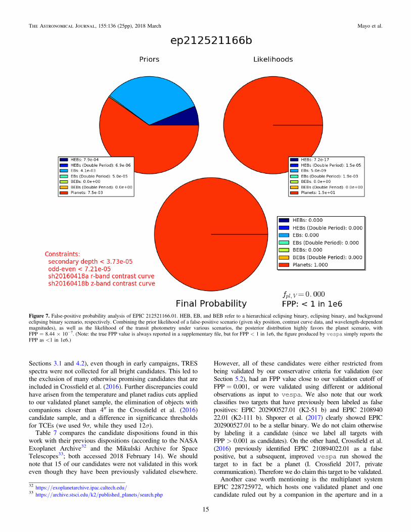
Upon its identification as a planet candidate, we observedEPIC 212521166 with the TRES spectrograph on the Mt.Hopkins 1.5 m Tillinghast reflector and with the DSSI speckle-imaging camera on the 3.5 m WIYN telescope at Kitt PeakNational Observatory. Using the orbital and transit parametersdetermined with our transit model, the stellar parametersderived from SPC, a folded light curve of the planetary transit,and two contrast curves in r band and z band collected via high-contrast speckle imaging from DSSI on the WIYN telescope(see Figure 6), vespa was employed to determine the FPP for

EPIC 212521166.01. The FPP was found to be 8.44×10−7,which was well below the cutoff threshold, so the planetcandidate was classified as validated. The key output figure ofvespa can be seen in Figure 7.Like us, Osborn et al. (2017) found EPIC 212521166 to be a

metal-poor K-dwarf star hosting planet candidate withP=13.9 day and Rp=2.6 R⊕. A comparison of planetaryand system parameters can be see in Table 6. Our analyses andtheirs are in good agreement for all parameters. Additionally,Osborn et al. (2017) took the further step of obtaining preciseRV observations to confirm the existence of EPIC212521166.01, so we can be confident that in this case, theassessment by vespa of a low FPP was well justified.

6.2. Full Validation Results

The process of validation described for EPIC 212521166.01in the previous section was similarly applied to the remainingcandidates suitable for validation. We identified 275 candidatesin 233 systems that had at least one usable TRES spectrum, andthe FPP was calculated for each of these candidates (seeTable 2).Occasionally, vespa failed to return an FPP; in such cases,

the lowest data point in the light curve was removed (to aid theinitialization process for the vespa trapezoidal transit fit), andvespa was rerun. This approach worked in most cases, but ifit failed, the lowest two data points were removed and vespawas rerun. If that was also unsuccessful, then the FPP was notreported. (Most of the time, vespa only failed after these stepsbecause of a Roche lobe overflow error.) 149 candidates in 111systems had an FPP<0.001 and were thus promoted tovalidated planet status.To date, the largest single release of K2 validation results has

been Crossfield et al. (2016), with 197 candidates and 104validated planets in C0–C4. In comparison, 108 of ourcandidates are from C0–C4, 69 of which are validated. Thetwo samples share 53 candidates in common, 37 of which arevalidated and 9 of which remain candidates in both analyses.(Additionally, 2 candidates in common are only validated inthis work, while 5 are only validated in Crossfield et al. 2016.)This leaves 55 candidates in our C0–C4 sample (30 of whichare validated) that were undetected by Crossfield et al. (2016),as well as 146 candidates (62 of which are validated) in theCrossfield et al. (2016) sample that are undetected in our ownC0–C4 sample. Only ∼21% of the total candidates weredetected by both analyses, and only ∼26% of the totalvalidated planets were validated by both analyses.The sample overlap may seem surprisingly small, but it

makes more sense when the candidate selection and validationprocesses are examined. For example, Crossfield et al. (2016)only considered candidates with 1 day<P<37 day (19% ofour C0–C4 sample was outside that range), and we onlyconsidered candidates with Kp<13 (48% of their sample wasoutside that range). If we only consider C0–C4 candidateswithin those ranges (137 total), both teams find over half ofeach other’s samples, and the overlap between samples rises to39% (53 candidates). Similarly, for validated planets withinthese ranges (77 total), both teams find more than two-thirds ofeach other’s samples, and the overlap between samples rises to57% (44 validated planets).There are many further examples of differences that created

discrepancies between the two samples. We required that eachplanet candidate had at least one usable TRES spectrum (see

14

The Astronomical Journal, 155:136 (25pp), 2018 March Mayo et al.

Sections 3.1 and 4.2), even though in early campaigns, TRESspectra were not collected for all bright candidates. This led tothe exclusion of many otherwise promising candidates that areincluded in Crossfield et al. (2016). Further discrepancies couldhave arisen from the temperature and planet radius cuts appliedto our validated planet sample, the elimination of objects withcompanions closer than 4″in the Crossfield et al. (2016)candidate sample, and a difference in significance thresholdsfor TCEs (we used 9σ, while they used 12σ).

Table 7 compares the candidate dispositions found in thiswork with their previous dispositions (according to the NASAExoplanet Archive32 and the Mikulski Archive for SpaceTelescopes33; both accessed 2018 February 14). We shouldnote that 15 of our candidates were not validated in this workeven though they have been previously validated elsewhere.

However, all of these candidates were either restricted frombeing validated by our conservative criteria for validation (seeSection 5.2), had an FPP value close to our validation cutoff ofFPP=0.001, or were validated using different or additionalobservations as input to vespa. We also note that our workclassifies two targets that have previously been labeled as falsepositives: EPIC 202900527.01 (K2-51 b) and EPIC 210894022.01 (K2-111 b). Shporer et al. (2017) clearly showed EPIC202900527.01 to be a stellar binary. We do not claim otherwiseby labeling it a candidate (since we label all targets withFPP>0.001 as candidates). On the other hand, Crossfield et al.(2016) previously identified EPIC 210894022.01 as a falsepositive, but a subsequent, improved vespa run showed thetarget to in fact be a planet (I. Crossfield 2017, privatecommunication). Therefore we do claim this target to be validated.Another case worth mentioning is the multiplanet system

EPIC 228725972, which hosts one validated planet and onecandidate ruled out by a companion in the aperture and in a

Figure 7. False-positive probability analysis of EPIC 212521166.01. HEB, EB, and BEB refer to a hierarchical eclipsing binary, eclipsing binary, and backgroundeclipsing binary scenario, respectively. Combining the prior likelihood of a false-positive scenario (given sky position, contrast curve data, and wavelength-dependentmagnitudes), as well as the likelihood of the transit photometry under various scenarios, the posterior distribution highly favors the planet scenario, withFPP=8.44×10−7. (Note: the true FPP value is always reported in a supplementary file, but for FPP<1 in 1e6, the figure produced by vespa simply reports theFPP as <1 in 1e6.)

32 https://exoplanetarchive.ipac.caltech.edu/33 https://archive.stsci.edu/k2/published_planets/search.php

15

The Astronomical Journal, 155:136 (25pp), 2018 March Mayo et al.

NESSI speckle image. The smallest aperture mask we testedexcluded the companion (located approximately 12 arcsec fromthe primary), but only exhibited transits for one of thecandidates, hence the difference in flags for the two candidates.

In addition to the FPPs and other parameters derived throughthe validation process described in previous sections, we alsocalculated the radii and masses of the stars in our sample (thestellar radius allowed us to calculate the absolute planetaryradius). We calculated these parameters by inputting stellareffective temperature, metallicity, and surface gravity into theisochrones Python package (Morton 2015a). We alsofound that inputting 2MASS photometry into isochronesalong with the aforementioned stellar parameters had no

noticeable effect on the resulting stellar radius and mass values(or their uncertainties). Although isochrones have been foundto underestimate stellar radii before (Dressing et al. 2017a,2017b; Martinez et al. 2017), this effect is confined to Mdwarfs and late-K dwarfs, which are largely excluded from ourhost star sample since we do not consider stars with effectivetemperatures below 4250 K (see Section 4.2). The derivedstellar masses and radii are reported in Table 2. (We also notethat all stellar parameters for each system are reported inTable 3.)

7. Discussion

7.1. Lessons Learned

There have been a few recent instances of false-positivemisclassification (Cabrera et al. 2017; Shporer et al. 2017), inwhich a target has been classified as a validated planet but waslater shown to be a false positive through subsequent analysis.Here, we discuss some of the pitfalls of statistical validation,and share some lessons we have learned and solutions we haveimplemented to prevent false-positive misclassification.First, spectroscopy is key. Stellar parameters are crucial to

understanding the host star and correctly classifying thecandidates. For example, identifying the star as highly evolvedcan prevent an orbiting brown dwarf or M dwarf from beingincorrectly labeled as a smaller planet orbiting a main-sequencestar. One might attempt to avoid this issue by estimating stellarsurface gravity via photometry alone, but that is notoriouslydifficult to do and can lead to incorrectly estimated stellarparameters. Collecting at least one spectrum from which toestimate spectroscopic parameters (including surface gravity)

Table 6System and Planetary Parameters of EPIC 212521166

Parameter Unit This Paper Osborn et al. (2017)

Orbital parametersPeriod P days 13.86391 0.00023

0.00022-+ 13.86375±2.6×10−4

Time of first transita BJD-2454833 2386.87440 0.000680.00072

-+ 2442.32992±6.1×10−4

Orbital eccentricity e L 0 (fixed) 0.079±0.07Inclination degrees 89.36 0.75

0.43-+ 89.35 0.24

0.41-+

Transit parametersSystem scale a/R* L 32.3 5.7

2.0-+ 30.8±1.0

Impact parameter b L 0.36 0.230.28

-+ 0.34 0.22

0.14-+

Transit duration T14 hr 3.181 0.0470.072

-+ 3.22±0.03

Radius ratio Rp/R* L 0.0334 0.00070.0018

-+ 0.0333±6.6×10−4

Planet parametersPlanet radius Rp R⊕ 2.52 0.10

0.16-+ 2.592±0.098

Stellar parameters

Stellar mass M* Me 0.724±0.025 0.738±0.018Stellar radius R* Re 0.692 0.023

0.025-+ 0.713±0.020

Effective temperature Teff K 4877±50 5010±50Surface gravity log g g cm−2 4.51±0.10 4.60±0.03Metallicity [m/H]b dex −0.30±0.08 −0.34±0.03

Validation parametersFPP L 8.44×10−7 L

Notes.a Our reported transit time and that reported by Osborn et al. (2017) differ by four orbital periods.b Our reported metallicity is [m/H] (derived from many metal absorption features), while the metallicity reported in Osborn et al. (2017) is [Fe/H] (derived from ironabsorption lines only).

Table 7Breakdown of Candidate Dispositions

Previous Updated Disposition

Dispositiona VP PC All

VP 53 15 68PC 39 55 94FP 1b 1c 2UK 56 55 111

All 149 126 275

Notes.a VP=Validated Planet, PC=Planet Candidate, FP=False Positive,UK=Unknown.b EPIC 210894022.01. See Section 6.2.c EPIC 202900527.01. See Section 6.2.

16

The Astronomical Journal, 155:136 (25pp), 2018 March Mayo et al.

can avoid many issues like this, and collecting more spectramay exclude (or reveal) large RV variations from an eclipsingbinary scenario.

Second, a search for secondary eclipses at all phases shouldbe performed to exclude a scenario with a highly eccentricbinary. The search method used here was the model-shiftuniqueness test designed by Coughlin et al. (2016). Thismethod compared off-transit portions of the light curve with thetransit portion of the best-fit transit model (and the transitmodel inverted, to provide a visual comparison of detectionsignificance). An even more rigorous method would considersecondary eclipses of duration and depth distinct from that ofthe transit.

Third, when validating exoplanets using vespa, one shouldbe very careful about which broadband photometry is used andwhat offsets and systematics there are. Statistical validationwork on data from the original Kepler mission took advantageof high-quality and uniform broadband photometry from theKepler Input Catalog (KIC, Brown et al. 2011). The analogousEPIC catalog for K2 is similarly vital to the analysis of the K2star and planet sample. However, it is approximately four timeslarger and was produced by collecting archival photometricmeasurements; therefore, it is more heterogeneous and moreprone to systematic errors and offsets than the KIC. We havefound that in some cases, these systematic errors or offsets inphotometry can result in untrustworthy FPP estimates, inparticular, extremely low FPP measurements for known orlikely false positives. For example, when we input to vespaall available broadband photometry from the EPIC catalog forthe candidate EPIC 211418290.01, vespa yielded an FPPlower than 10−6 because it was unable to find an acceptable fitto a binary star model due to underestimated photometricuncertainties and therefore incorrectly ruled this false-positivescenario out. However, inputting only 2MASS photometry tovespa yielded a better fit to the eclipsing binary scenario, andvespa therefore returned a much higher FPP of about 0.6.Situations like this were not uncommon, which is why weultimately decided to use only photometry from the all sky2MASS survey. We chose to use only the 2MASS surveybecause it provides broadband photometry for all of ourcandidates and operates in the infrared, reducing the effects ofreddening. Including photometry from additional surveys thatare calibrated differently and have distinct systematic uncer-tainties would introduce non-uniformities that would bedifficult to quantify and could bias our results.

To be conservative, we also added 0.02 mag of systematicerror in quadrature with the reported error for each 2MASSband we used. This will continue to be important after thelaunch of TESS, which will observe targets selected from theTESS Input Catalog (TIC, Stassun et al. 2017). The TIC will bevery important for selecting candidates for observation andfollow-up; however, it is being assembled in a manner similarto the EPIC and is approximately 10 times larger, so it mayhave similar or even greater photometric offsets.

Fourth, it is very important to make and remake a candidate’slight curve with multiple apertures of varying sizes, in order todetermine whether the transit signal originates from the target staror a nearby background star (and thus exclude background false-positive scenarios). This test caught many false positives in ourown analysis, and has been used successfully before in othercandidacy analyses (e.g., Dressing et al. 2017b).

Fifth, transiting giant planets are nearly indistinguishablefrom eclipsing brown dwarfs or small M-dwarf stars, since theyhave roughly equal radii. Great care should be taken wheninterpreting the output of vespa for giant planets, and unlessthere is a clear way to distinguish between the two scenarios(via RV measurements, secondary eclipse detection, compositespectra, etc.), attempts to validate large planets can be difficultand prone to error.By considering each of the above lessons and incorporating

them into future validation analyses, misclassifications ofvalidated planets can be significantly reduced and hopefullyeliminated in all but the most perverse scenarios.We now investigate some of the individual validated planets

in our sample as well as the characteristics of our sample as awhole.

7.2. A New Brightest Host Star in the K2 and Kepler PlanetSamples

One interesting target in our sample is EPIC 205904628(HIP 110758, HD 212657), an F7 star observed in Campaign 3.We detected and validated a 2.8 R⊕ planet on a 10-day orbit. Ata V magnitude of 8.24, EPIC 205904628 is now the brighteststar at optical wavelengths in the entire Kepler and K2 samplesto host a validated planet. EPIC 205904628 is just slightlybrighter than Kepler-21 (V=8.25), a star of similar spectraltype found during the original Kepler mission to host a singleshort-period exoplanet (Howell et al. 2012; López-Moraleset al. 2016). TESS is expected to discover planets around manystars this bright and brighter.We note that due to its brightness, we applied some special

care to this star. In particular, we re-reduced the K2 light curveby extracting light curves from larger photometric aperturesthan our standard pipeline uses. We also incorporatedinformation from 2MASS J-band imaging to rule out additionalstars in the photometric aperture by calculating a contrast curveand inputting it to vespa to provide deeper imagingconstraints than our speckle image.

7.3. Characteristics of the Sample

In addition to individual planets in our sample, it isinteresting to explore a few of the demographics of the newlyvalidated exoplanet population. Figures 8–15 reveal variousaspects of the validated exoplanet sample and the exoplanetcandidate sample.

7.3.1. The Stellar Magnitude Distribution

Figure 8 is a histogram of the distribution of brightnesses forthe host stars in our sample compared with the brightness forstars hosting known Kepler planets (downloaded from https://exofop.ipac.caltech.edu/; accessed 2017 December 4). Most ofthe candidates in our population are clustered near stellarmagnitudes of Kp= 12 to Kp= 13, and the cutoff we imposedat Kp= 13 is very evident. Figure 8 shows the distribution ofbrightnesses for host stars to known Kepler planets. Thisdistribution peaks near Kp= 15 and drops rapidly at brightermagnitudes. It is more difficult to find planet candidates aroundfaint targets for K2 than for Kepler since the baseline is shorter.Therefore K2 candidates tend to orbit very bright host starsrelative to Kepler candidates, making K2 candidates excellenttargets for follow-up observations.

17

The Astronomical Journal, 155:136 (25pp), 2018 March Mayo et al.

7.3.2. The Effective Temperature Distribution

Most of the validated planets and candidates we identifiedorbit host stars with effective temperatures in the 5000–6000 Krange. However, out of 233 stars in our sample 41 are coolerthan 5000 K and 25 are hotter than 6000 K. No stars in oursample are cooler than 4250 K or hotter than 6500 K. SeeFigure 9 for a comparison with the Kepler sample (downloadedfrom https://exofop.ipac.caltech.edu/; accessed 2017 Decem-ber 4).

7.3.3. The Period Distribution

We also explored the period distribution of our candidatepopulation. As can be seen in Figure 10, the typical validatedplanet or candidate has an orbital period of 20 days or less. Thisshould come as no surprise, given the baseline of ∼75 days ofK2 observations per campaign field. Of 275 candidates in oursample, only 46 have periods longer than 20 days, and only 10have periods longer than 40 days.

7.3.4. The Multiplicity Distribution

Most of the candidates in our sample (validated or otherwise)are the only candidate in their system to have been detected.However, our sample does include 21 systems with two

candidates (15 of these have only validated planets), 9 systemswith three candidates (8 of those have only validated planets),and 1 system with four candidates (EPIC 212157262; allcandidates in this system are validated). The full multiplicitydistribution can be seen in Figure 11.

Figure 8. Histograms of the Kepler magnitude for host stars to validatedplanets (purple) and candidate planets (diagonal lines) from C0–C10 of K2 thathave been identified in this work, as well as a comparison with host stars toconfirmed Kepler planets (pink). There is a fairly sharp cutoff in our samplenear magnitude 13, since validation was only conducted on stars for which wehad a spectrum and almost all of the spectra we used were for targets brighterthan 13 mag. The typical Kepler host star is much fainter, with the peak of thedistribution near 15 mag, which makes K2 target stars much more suitable forfollow-up observations than Kepler stars. Moreover, the brightest star hosting avalidated planet in our sample is EPIC 205904628, a V=8.2 star with a2.8 R⊕ planet on a 10-day orbit. Validated in this work, EPIC 205904628 isnow the brightest host star for a validated planet in either the Kepler or K2samples.

Figure 9. Histograms of the effective temperature for host stars to validatedplanets (purple) and candidate planets (diagonal lines) from C0–C10 of K2 thathave been identified in this work, as well as a comparison with host stars toconfirmed Kepler planets (pink). Except for the cutoffs we impose atTeff=4250 and 6500 K, our sample follows a similar effective temperaturedistribution as the Kepler sample.

Figure 10. Histogram of the orbital period for the validated planets (purple)and candidates (diagonal lines) in C0–C10 of K2 that have been identified inthis work. The steep drop-off in validated planets and candidates at around20 days is due to the K2 strategy of observing each field for only ∼75 days.

18

The Astronomical Journal, 155:136 (25pp), 2018 March Mayo et al.

7.3.5. The Planet Radius Distribution

One of the more interesting features of our sample was theradius distribution. Figure 12 demonstrates the full planetaryradius distribution of our sample for both validated planets andcandidates. As expected, there is a sharp cutoff in planet radiusfor validated planets at Rp=8 R⊕(since we generally chosenot to validate larger planets).

In order to investigate the radius distribution of theunderlying planet population, we adopted and applied a roughcompleteness correction to our planet sample. We determinedthe completeness of our K2 planet detection pipeline byperforming injection/recovery tests. We injected planet signalsinto K2 light curves over a range of expected S/Ns (analogousto the injection/recovery tests performed by Petigura et al.2013; Dressing & Charbonneau 2015; Christiansen et al. 2016on the Kepler pipeline). We then calculated for each of ourplanet candidates the number of stars observed by K2 aroundwhich we could have detected the candidate, and weighted thecontribution of each candidate to the histograms by that factorand the geometric transit probability.

The uncorrected and corrected distributions for validatedplanets and candidates can be seen in Figure 13, while acomparison of our corrected candidate sample to the Fultonet al. (2017) sample and a log-uniform distribution can be seenin Figure 14. Additionally, a completeness-corrected contourplot of stellar incident flux versus planetary radius for ourcandidate sample can be seen in Figure 15 (constructed in thesame way as Figure10 from Fulton et al. 2017).

By visual inspection of these figures alone, our correctedcandidate sample appears to exhibit a gap in the radiusfrequency around 1.8–2.0 R⊕, similar to the gap in the Keplerplanet sample explored by Fulton et al. (2017). They arguedthat the underlying astrophysical effect could be

photoevaporation, whereby stellar incident flux strips a planet’sH/He atmosphere if the atmosphere is not thick enough,leaving a population of stripped, rocky planets and anuntouched population of larger, gaseous mini-Neptunes (Owen& Wu 2013; Lopez & Rice 2016; Owen & Wu 2017; VanEylen et al. 2017). As an alternative hypothesis, they alsosuggested that gas accretion could be delayed during planetformation until the protoplanetary disk is already gas poor,creating a population of small, rocky planets (Lee et al. 2014;Lee & Chiang 2016).We wished to analyze in a more quantitative fashion how the

completeness-corrected radius distribution of our K2 candidatescompared to the completeness-corrected Kepler candidatesfrom Fulton et al. (2017); we also decided to compare with alog-uniform distribution to probe the significance of a possiblebimodality (as did Fulton et al. 2017). We binned all threenormalized distributions in 0.1 R⊕ intervals from 1.2 to 2.5 R⊕.We assigned error bars to our own sample and the Fulton et al.(2017) sample via Poisson statistics (for the number ofcandidates in each bin) and then scaled the uncertaintyaccording to the completeness-correction scaling applied toeach bin.We then calculated reduced

2c between our sample and that ofFulton et al. (2017) as well as our sample and the log-uniformdistribution, finding values of 2.21 and 2.34, respectively.Across all bin numbers from 5 to 20 for which there were morethan two candidates in every (equally sized and spaced) bin forall samples, the average reduced

2c was 2.21 between our sampleand that of Fulton et al. (2017) and 2.95 between our sampleand the log-uniform distribution. However, we note that a largeportion of the reduced

2c between our sample and that of Fultonet al. (2017) is caused by only the smallest radius bin. Still, theFulton et al. (2017) sample did not provide a significantimprovement in goodness of fit than a simple log-uniform

Figure 11. Histogram of the multiplicity for the validated planet systems(purple) and planet candidate systems (diagonal lines) in C0–C10 of K2 thathave been identified in this work. (A validated planet system is a system forwhich all candidates have been validated.) Most validated planets andcandidates have no detected candidate companions in their system. The largestsystem in the sample is EPIC 212157262, which hosts four validated planets.

Figure 12. Histogram of the planetary radius for the validated planets (purple)and candidates (diagonal lines) in C0–C10 of K2 that have been identified inthis work. See Figures 13 and 14 for narrower ranges, a completenesscorrection, and a comparison with the Fulton et al. (2017) planet candidatesample.

19

The Astronomical Journal, 155:136 (25pp), 2018 March Mayo et al.

distribution. This suggests that the visual gap in our candidatesample cannot be quantitatively confirmed unless futureobservations and planet detections are made to increase thesample size.

7.3.6. Future Applications

The K2 mission has thus far conducted observations throughmore than 15 campaigns, and it will continue observations forfuture campaigns until it expends all of its fuel. Given that thevalidation infrastructure built for this research is directlyapplicable to future campaigns, we will be able to identify andvalidate exoplanet candidates from upcoming campaigns asquickly as the necessary follow-up observations can becollected.

This research will also be useful even after the end of the K2mission. The upcoming TESS mission (Ricker et al. 2015) isexpected to yield more than 1500 total exoplanet discoveries,but it is also estimated that TESS will detect over 1000 false-positive signals (Sullivan et al. 2015). Even so, one (out ofthree) of the level-one baseline science requirements for TESSis to measure the masses of 50 planets with Rp<4 R⊕.Therefore, an extensive follow-up program to the primaryphotometric observations conducted by the spacecraft isrequired, including careful statistical validation to aid in theselection of follow-up targets. The work presented here will beextremely useful in that follow-up program, since only modestadjustments will allow for the validation of planet candidatesystems identified by TESS rather than K2.

8. Summary and Conclusions

In this paper, we processed 208,423 targets from C0–C10,removed instrumental systematics from the K2 photomtry, andsearched for TCEs. We identified ∼30,000 TCEs, which weresubjected to triage and vetting. Of these, ∼1000 target systemspassed both procedures and were upgraded to candidates. Ofthese, 275 candidates in 233 systems had at least one usableTRES spectrum. For each candidate, we also collected and

analyzed follow-up observations, including spectroscopy andhigh-contrast imaging. We derived transit/orbital parametersfrom the K2 photometry, stellar parameters from the spectra,and contrast curves from the high-contrast imaging. Then,using these results, we determined the FPP of each planetcandidate using the vespa validation procedure (Morton2012, 2015b), which calculates the likelihood of various false-positive scenarios as well as the true-positive scenario. TheseFPP values were then adjusted appropriately for systems withradial velocity measurements and for multiplanet systems (seeSection 5.1). We reported the resulting FPPs for our planetcandidates (see Table 2) and classified candidates withFPP<0.001 as validated planets.Of the 275 candidates, 149 had an FPP below the validation

threshold of 0.001, while 126 remained candidates (FPP>0.001). According to the NASA Exoplanet Archive34 and theMikulski Archive for Space Telescopes35 (both accessed 2018February 14), of the 149 newly validated exoplanets, 56 havenot been previously detected, 39 have been identified ascandidates, 53 have been validated, and 1 has previously beenclassified as a false positive (EPIC 210894022.01; seeSection 6.2). As a result, this work will increase the validatedK2 planet sample by nearly 50% (and increase the K2 candidatesample by ∼20%). The full disposition results can be found inTable 7.Most of the newly validated exoplanets orbited host stars

with 12<Kp< 13 and 5000 K<Teff< 6000 K. Additionally,the majority of validated planets had orbital periods <20 daysand planetary radii between 1 and 4 R⊕. Our completecandidate sample also shows signs of a frequency gap in theradius distribution (see Figure 14), similar to the gap found byFulton et al. (2017). However, further analysis with a largerplanet sample is required to confirm the radius gap for K2planets.

Figure 13. Left: histogram of planetary radius for the validated planets (purple) and candidates (diagonal lines) in C0–C10 of K2 that have been identified in this work(between 0.7 and 12 R⊕). Right: same data as presented in the left panel, with a completeness correction applied to estimate the underlying planet population. Errorbars for each bin correspond to n1 (where n is the number of objects in the bin) scaled according to the completeness correction subsequently performed. Throughvisual inspection, the full candidate sample appears to exhibit a frequency gap centered near 1.8–2.0 R⊕.

34 https://exoplanetarchive.ipac.caltech.edu/35 https://archive.stsci.edu/k2/published_planets/search.php

20

The Astronomical Journal, 155:136 (25pp), 2018 March Mayo et al.

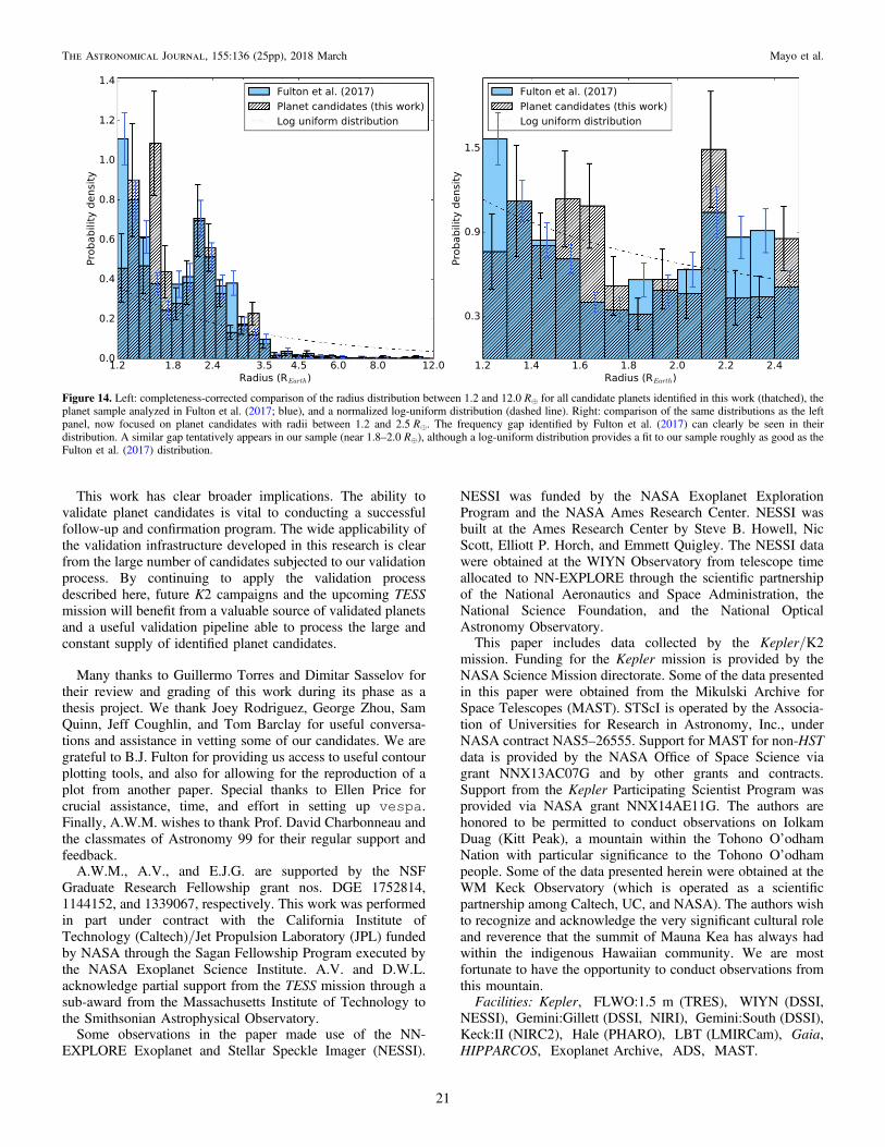
This work has clear broader implications. The ability tovalidate planet candidates is vital to conducting a successfulfollow-up and confirmation program. The wide applicability ofthe validation infrastructure developed in this research is clearfrom the large number of candidates subjected to our validationprocess. By continuing to apply the validation processdescribed here, future K2 campaigns and the upcoming TESSmission will benefit from a valuable source of validated planetsand a useful validation pipeline able to process the large andconstant supply of identified planet candidates.

Many thanks to Guillermo Torres and Dimitar Sasselov fortheir review and grading of this work during its phase as athesis project. We thank Joey Rodriguez, George Zhou, SamQuinn, Jeff Coughlin, and Tom Barclay for useful conversa-tions and assistance in vetting some of our candidates. We aregrateful to B.J. Fulton for providing us access to useful contourplotting tools, and also for allowing for the reproduction of aplot from another paper. Special thanks to Ellen Price forcrucial assistance, time, and effort in setting up vespa.Finally, A.W.M. wishes to thank Prof. David Charbonneau andthe classmates of Astronomy 99 for their regular support andfeedback.

A.W.M., A.V., and E.J.G. are supported by the NSFGraduate Research Fellowship grant nos. DGE 1752814,1144152, and 1339067, respectively. This work was performedin part under contract with the California Institute ofTechnology (Caltech)/Jet Propulsion Laboratory (JPL) fundedby NASA through the Sagan Fellowship Program executed bythe NASA Exoplanet Science Institute. A.V. and D.W.L.acknowledge partial support from the TESS mission through asub-award from the Massachusetts Institute of Technology tothe Smithsonian Astrophysical Observatory.

Some observations in the paper made use of the NN-EXPLORE Exoplanet and Stellar Speckle Imager (NESSI).

NESSI was funded by the NASA Exoplanet ExplorationProgram and the NASA Ames Research Center. NESSI wasbuilt at the Ames Research Center by Steve B. Howell, NicScott, Elliott P. Horch, and Emmett Quigley. The NESSI datawere obtained at the WIYN Observatory from telescope timeallocated to NN-EXPLORE through the scientific partnershipof the National Aeronautics and Space Administration, theNational Science Foundation, and the National OpticalAstronomy Observatory.This paper includes data collected by the Kepler/K2

mission. Funding for the Kepler mission is provided by theNASA Science Mission directorate. Some of the data presentedin this paper were obtained from the Mikulski Archive forSpace Telescopes (MAST). STScI is operated by the Associa-tion of Universities for Research in Astronomy, Inc., underNASA contract NAS5–26555. Support for MAST for non-HSTdata is provided by the NASA Office of Space Science viagrant NNX13AC07G and by other grants and contracts.Support from the Kepler Participating Scientist Program wasprovided via NASA grant NNX14AE11G. The authors arehonored to be permitted to conduct observations on IolkamDuag (Kitt Peak), a mountain within the Tohono O’odhamNation with particular significance to the Tohono O’odhampeople. Some of the data presented herein were obtained at theWM Keck Observatory (which is operated as a scientificpartnership among Caltech, UC, and NASA). The authors wishto recognize and acknowledge the very significant cultural roleand reverence that the summit of Mauna Kea has always hadwithin the indigenous Hawaiian community. We are mostfortunate to have the opportunity to conduct observations fromthis mountain.Facilities: Kepler, FLWO:1.5 m (TRES), WIYN (DSSI,

NESSI), Gemini:Gillett (DSSI, NIRI), Gemini:South (DSSI),Keck:II (NIRC2), Hale (PHARO), LBT (LMIRCam), Gaia,HIPPARCOS, Exoplanet Archive, ADS, MAST.

Figure 14. Left: completeness-corrected comparison of the radius distribution between 1.2 and 12.0 R⊕ for all candidate planets identified in this work (thatched), theplanet sample analyzed in Fulton et al. (2017; blue), and a normalized log-uniform distribution (dashed line). Right: comparison of the same distributions as the leftpanel, now focused on planet candidates with radii between 1.2 and 2.5 R⊕. The frequency gap identified by Fulton et al. (2017) can clearly be seen in theirdistribution. A similar gap tentatively appears in our sample (near 1.8–2.0 R⊕), although a log-uniform distribution provides a fit to our sample roughly as good as theFulton et al. (2017) distribution.

21

The Astronomical Journal, 155:136 (25pp), 2018 March Mayo et al.

AppendixCalibrating TRES to Measure the Mt. Wilson SHK Index

Our work involved the analysis of many spectra collectedwith the TRES on the 1.5m Tillinghast telescope at theWhipple Observatory on Mt. Hopkins. In addition to usingTRES spectra to derive spectroscopic parameters and measureradial velocities, we also used TRES to measure the Mt. WilsonSHK activity indicator. SHK is a ratio between the flux in thecores of the calcium II H and K spectral features (at3933.66± 1.09 and 3968.47± 1.09Å) and the flux in twonearby continuum regions (one slightly redward of the Ca IIlines, called R, and one slightly blueward, called V). SHK iscommonly used as a proxy for a star’s chromospheric activity(Isaacson & Fischer 2010). Because SHK depends on ratios offluxes at different wavelengths, it is sensitively affected by thespectrograph blaze function. The effect of the spectrographblaze function must therefore be carefully calibrated andquantified in order to standardize measurements of SHK fromdifferent instruments. In this Appendix, we describe how wecalibrated the TRES spectrograph to place measurements ofSHK on the Mt. Wilson scale, and present our measurements ofSHK for a handful of bright K2 planet candidate hosts for whichwe were able to measure SHK reliably. These measurements arelisted in Table 4.

To calibrate TRES to measure SHK on the Mt. Wilson scale,we closely followed the procedure of Isaacson & Fischer(2010). We based our calibration on a sample of stars that wereboth observed by TRES (prior to 2016 June 1) and wereincluded in the Duncan et al. (1991) catalog of Mt. Wilson SHKmeasurements. Additionally, the following cuts were applied toimprove the sample quality:

1. TRES spectra for the star in question were only used ifthe photon count in the R continuum region(4001.07± 10Å) was greater than 174,000. (The cutoffis at 150,000 ADU, which is converted using a gain of1.16 for TRES.) This conservative cutoff was imposed toremove spectra with only low or moderate S/N from thecalibration.

2. The star was not in a close binary or multiple system. Weonly included widely separated (5″) visual binaries inorder to prevent flux from the companion star(s) beingblended with flux of the intended target.

3. One fast-rotating star (HD 30780, or “VB123” in the TRESdatabase) was removed from the calibration set as the Hand K emission cores were clearly broadened and smearedwith other spectral features (vsini;180 km s−1).

After these cuts, our calibration sample included 118 starswith a total of 1204 individual TRES observations. Thecalibration was made in the same way as in Isaacson & Fischer(2010), by determining values of Kcoeff, Vcoeff, m, and b thatminimize the differences between the Mt. Wilson surveymeasurement of SHK for each star (Duncan et al. 1991) and SHKcalculated from the TRES spectra using the following equation:

S mH K K

R V Vb, 1HK,TRES

coeff

coeff= ´

++

+ ( )

where H and K are fluxes in the cores of the Ca II H and Klines,36 R and V are continuum fluxes,37 Kcoeff is a coefficientthat scales the magnitude of K fluxes to match the magnitude ofH fluxes, Vcoeff is a coefficient that scales the magnitude of Vfluxes to match the magnitude of R fluxes, and m and b are freeparameters.Kcoeff was calculated through a linear regression between H

and K for our TRES spectra, so as to scale the magnitude of Kto match that of H. The same process was performed for R andV in order to calculate Vcoeff. This was done to mirror theapproach taken by Isaacson & Fischer (2010) in theircalibration of the Keck HIRES instrument.We estimated m and b by minimizing the differences

between SHK,Mt.Wilson from the Mt. Wilson survey (Duncanet al. 1991) and SHK,TRES determined from TRES spectra withEquation (1) using an MCMC algorithm with affine-invariantensemble sampling (Foreman-Mackey et al. 2013). Wecalculated the likelihood, , using the following function:

S Sln 0.5 ln , 2HK HK,TRES ,Mt.Wilson

2

22 å s

s= --

+⎛⎝⎜

⎞⎠⎟( ) ( ) ( )

Figure 15. Left: contour plot of incident stellar flux vs. planetary radius. The black points are the 275 candidates in our sample, and the typical uncertainty is plotted inthe top left. The contours are completeness-corrected and roughly scaled to the same height as those in Figure 10 from Fulton et al. (2017). The contours showtentative visual evidence of a gap in the radius frequency near 1.6–1.8 R⊕. Right: top panel of Figure10 from (Fulton et al. 2017; reproduced with permission), with asimilar gap near 1.6–1.8 R⊕.

36 The H and K fluxes were calculated by integrating the spectrum overtriangular-shaped bandpasses centered at 3933.66 and 3968.47 Å, respectively,each with an FWHM of 1.09 Å.37 The R and V fluxes were calculated by integrating the spectrum over 20 Åwide box-shaped bandpasses centered at 4001.07 and 3901.07 Å, respectively,following Duncan et al. (1991).

22

The Astronomical Journal, 155:136 (25pp), 2018 March Mayo et al.

where σ is a jitter term that absorbs uncertainties both inmeasurements of SHK and in their uncertainties due to factorsincluding astrophysical variability in the SHK index of a singlestar over time. We imposed uniform priors on m and b, andimposed a Jeffreys prior on σ.

It is important to note that there might be both multipleTRES spectra and multiple Mt. Wilson SHK measurements for agiven star. So if a star had more than one TRES spectrum orMt. Wilson SHK measurement, this star was simply representedas a grid of TRES and Mt. Wilson measurements in the MCMCprocess. With this in mind, the total number of data points inthe fitting process was 3108. This implicitly gives higherweight in our calibration to stars with multiple observations,which helps average out astrophysical variability in SHK.

Our MCMC process used 200 chains of 50,000 steps each inorder to explore parameter space and determine best-fitparameters and uncertainties. The resulting ensemble was wellconverged according to the Gelman–Rubin statistic (Gelman &Rubin 1992), which in this case was lower than 1.04 for allparameters. The last 500 samples of the MCMC process arevisualized in Figure 16 with a posterior corner plot (Foreman-Mackey 2016). We found the following parameter values fromour model fit:

K 0.876coeff =V 0.775coeff =

m 15.496 0.0690.068= -

+

b 0.0031 0.0015= - ln jitter 3.119 0.013.= - ( )

There was also significant covariance between m and b(see Figure 16), which we estimated to be m bCov , =( )

8.571 10 5- ´ - .Statistical uncertainties, σrandom, for SHK were calculated by

propagating sample draws from four Poisson distributions

representing R, V, H, and K through draws from the m and bposterior distributions and the Kcoeff and Vcoeff values. We alsoincluded a systematic error term, σsystematic, in our uncertaintyestimates. We estimated the systematic uncertainties for TRESSHK measurements using six spectra with high S/N of thebright star Tau Ceti collected with TRES on the night of 2013October 24. We assumed that SHK for Tau Ceti remainedconstant over the course of a single night, and estimated asystematic error term based on the scatter between individualSHK measurements. Our final error estimates, σtotal, came fromassuming that the statistical uncertainties and systematicuncertainties were independent and could be added inquadrature as follows:

. 3total2

systematic2

random2s s s= + ( )

We note that our calibration for SHK is only valid overspecific ranges in parameter values. Our calibration wasperformed over a range of 0.244–1.629 in B−V and yieldedSHK values ranging from 0.055 to 2.070. Based on tests withsimulated data and with real data with low S/N, we arecautious of SHK measurements on spectra with fewer than290,000 photon counts (or 250,000 ADU) in the R and Vcontinuum regions combined. We also note that SHK measure-ments can be affected by rapid stellar rotation. We found byartificially broadening the lines of slowly rotating stars that SHKmeasurements for stars with vsini above 20 km s−1 can beskewed compared to the values that would have been measuredif the stars were rotating slowly.We tested our calibration by comparing SHK measurements

derived from TRES with a test set of SHK measurements fromthe literature (in particular, we focused on stars observed byIsaacson & Fischer 2010). We constructed the test data set byidentifying stars observed by TRES with the followingproperties:

1. The stars were not included in our calibration set (starsobserved both by Duncan et al. (1991) and TRES).

2. The TRES spectra for the star in question have photoncounts in the R continuum region greater than 174,000 (or150,000 ADU).

3. The star had at least one SHK measurement from KeckHIRES that had been reported in Isaacson &Fischer (2010).

After applying these cuts, we were left with a test set of 121stars, which had been observed a total of 4308 times by TRES.We show the results of our SHK calibration in Figure 17,

which compares TRES SHK measurements from our calibrationset with measurements from the Mt. Wilson survey, and inFigure 18, which compares TRES SHK measurements from ourtest set with values from Isaacson & Fischer (2010).For the calibration set, there is an 10.9% fractional rms

scatter about the one-to-one line. The only noticeable outlierappears to be at approximately (0.9, 0.2), corresponding to thesingle TRES spectrum (and Mt. Wilson measurement) of HD120477, a variable star observed in 2015 July by TRES andobserved no later than 1991 at Mt. Wilson. The reason for thisoutlier could not be identified, but its presence in the calibrationset did not significantly change the calibration, so it was left in(removing the point maintained a fractional rms scatterof 10.9%.)As for the test set, there is a 13.6% fractional rms scatter

about the one-to-one line, slightly larger than for the calibration

Figure 16. Corner plot for three parameters in our calibration of the TillinghastReflector Echelle Spectrograph for SHK, an indicator of stellar activity: a lineslope (m) and a line y-intercept (b) in our SHK equation, and a noise parameter(ln s( )) to account for error bars and stellar variability.

23

The Astronomical Journal, 155:136 (25pp), 2018 March Mayo et al.

set (which is to be expected). There does appear to a slightsystematic offset between TRES and Keck HIRES such thatSHK values from Keck HIRES tend to be lower than those fromTRES. However, this is to be expected, since the samesystematic underestimation with Keck HIRES compared to Mt.Wilson can be seen in Figure4 of Isaacson & Fischer (2010).There are also a few obviously errant data points in this figure,centered around (1.5, 0.5). These data points correspond to fourTRES spectra of the star GJ 570B, a spectroscopic binary. Thetest data set, because it was not used for calibration, was notclipped of binary stars; thus, GJ 570B is a clear example ofhow calculating SHK for close binaries can go wrong. However,the presence of those four spectra has very little effect on theresults; removing them only reduced the fractional rms scatterof the test set to 13.5%.

ORCID iDs

Andrew W. Mayo https://orcid.org/0000-0002-7216-2135Andrew Vanderburg https://orcid.org/0000-0001-7246-5438David W. Latham https://orcid.org/0000-0001-9911-7388Allyson Bieryla https://orcid.org/0000-0001-6637-5401Timothy D. Morton https://orcid.org/0000-0002-8537-5711Lars A. Buchhave https://orcid.org/0000-0003-1605-5666Courtney D. Dressing https://orcid.org/0000-0001-8189-0233Michael L. Calkins https://orcid.org/0000-0002-2830-5661David R. Ciardi https://orcid.org/0000-0002-5741-3047Gilbert A. Esquerdo https://orcid.org/0000-0002-9789-5474Mark E. Everett https://orcid.org/0000-0002-0885-7215Lea A. Hirsch https://orcid.org/0000-0001-8058-7443Elliott P. Horch https://orcid.org/0000-0003-2159-1463Andrew W. Howard https://orcid.org/0000-0001-8638-0320Steve B. Howell https://orcid.org/0000-0002-2532-2853John Livingston https://orcid.org/0000-0002-4881-3620Rahul Patel https://orcid.org/0000-0002-5025-6827Erik A. Petigura https://orcid.org/0000-0003-0967-2893Nicholas J. Scott https://orcid.org/0000-0003-1038-9702Evan Sinukoff https://orcid.org/0000-0002-5658-0601Jennifer G. Winters https://orcid.org/0000-0001-6031-9513

References

Adams, E. R., Jackson, B., & Endl, M. 2016, AJ, 152, 47Barros, S. C. C., Demangeon, O., & Deleuil, M. 2016, A&A, 594, A100Batalha, N. M., Borucki, W. J., Koch, D. G., et al. 2010a, ApJL, 713, L109Batalha, N. M., Rowe, J. F., Gilliland, R. L., et al. 2010b, ApJL, 713, L103Borucki, W., Koch, D., Basri, G., et al. 2008, in IAU Symp. 249, Exoplanets:

Detection, Formation and Dynamics (Cambridge: Cambridge Univ.Press), 17

Brown, T. M., Latham, D. W., Everett, M. E., & Esquerdo, G. A. 2011, AJ,142, 112

Buchhave, L. A., Latham, D. W., Johansen, A., et al. 2012, Natur, 486, 375Cabrera, J., Barros, S. C. C., Armstrong, D., et al. 2017, arXiv:1707.08007Carter, J. A., Fabrycky, D. C., Ragozzine, D., et al. 2011, Sci, 331, 562Christiansen, J. L., Clarke, B. D., Burke, C. J., et al. 2016, ApJ, 828, 99Christiansen, J. L., Vanderburg, A., Burt, J., et al. 2017, AJ, 154, 122Ciardi, D. R., Beichman, C. A., Horch, E. P., & Howell, S. B. 2015, ApJ,

805, 16Coughlin, J. L., Mullally, F., Thompson, S. E., et al. 2016, ApJS, 224, 12Coughlin, J. L., Thompson, S. E., Bryson, S. T., et al. 2014, AJ, 147, 119Crossfield, I. J. M., Ciardi, D. R., Isaacson, H., et al. 2017, AJ, 153, 255Crossfield, I. J. M., Ciardi, D. R., Petigura, E. A., et al. 2016, ApJS, 226, 7Crossfield, I. J. M., Petigura, E., Schlieder, J. E., et al. 2015, ApJ, 804, 10Cutri, R. M., Skrutskie, M. F., van Dyk, S., et al. 2003, yCat, 2246, 0David, T. J., Hillenbrand, L. A., Petigura, E. A., et al. 2016, Natur, 534, 658Dressing, C. D., & Charbonneau, D. 2015, ApJ, 807, 45Dressing, C. D., Newton, E. R., Schlieder, J. E., et al. 2017a, ApJ, 836, 167Dressing, C. D., Vanderburg, A., Schlieder, J. E., et al. 2017b, AJ, 154, 207Duncan, D. K., Vaughan, A. H., Wilson, O. C., et al. 1991, ApJS, 76, 383Foreman-Mackey, D. 2016, JOSS, 1, 24Foreman-Mackey, D., Hogg, D. W., Lang, D., & Goodman, J. 2013, PASP,

125, 306Foreman-Mackey, D., Montet, B. T., Hogg, D. W., et al. 2015, ApJ, 806, 215Fulton, B. J., Petigura, E. A., Howard, A. W., et al. 2017, AJ, 154, 109Furlan, E., Ciardi, D. R., Everett, M. E., et al. 2017, AJ, 153, 71Gaia Collaboration, Brown, A. G. A., Vallenari, A., et al. 2016a, A&A,

595, A2Gaia Collaboration, Prusti, T., de Bruijne, J. H. J., et al. 2016b, A&A, 595, A1Gelman, A., & Rubin, D. B. 1992, StaSc, 7, 457Goodman, J., & Weare, J. 2010, Commun. Appl. Math. Comput. Sci., 5, 65Hayward, T. L., Brandl, B., Pirger, B., et al. 2001, PASP, 113, 105Hirano, T., Dai, F., Gandolfi, D., et al. 2017, arXiv:1710.03239Hirsch, L. A., Ciardi, D. R., Howard, A. W., et al. 2017, AJ, 153, 117Hodapp, K.-W., Irwin, E. M., Yamada, H., et al. 2003, Proc. SPIE, 4841, 869Horch, E. P., Veillette, D. R., Baena Gallé, R., et al. 2009, AJ, 137, 5057Howell, S. B., Everett, M. E., Sherry, W., Horch, E., & Ciardi, D. R. 2011, AJ,

142, 19

Figure 17. Comparison of our SHK calibration for TRES with the Duncan et al.(1991) catalog for our calibration data set of 118 stars (with 1204 TRESspectra). Each red point denotes a unique pair of observations from TRES andMt. Wilson for a given star. The fractional rms scatter on the calibration setis 11.0%.

Figure 18. Comparison of our SHK calibration for TRES with the Isaacson &Fischer (2010) catalog for our test data set of 121 stars (with 4308 TRESspectra). Each red point denotes a unique pair of observations from TRES andMt. Wilson for a given star. The fractional rms scatter on the calibration setis 13.6%.

24

The Astronomical Journal, 155:136 (25pp), 2018 March Mayo et al.

Howell, S. B., Rowe, J. F., Bryson, S. T., et al. 2012, ApJ, 746, 123Howell, S. B., Sobeck, C., Haas, M., et al. 2014, PASP, 126, 398Huber, D., Bryson, S. T., Haas, M. R., et al. 2016, ApJS, 224, 2Isaacson, H., & Fischer, D. 2010, ApJ, 725, 875Jenkins, J. M., Caldwell, D. A., Chandrasekaran, H., et al. 2010, ApJL,

713, L87Kipping, D. M. 2013, MNRAS, 435, 2152Kovács, G., Zucker, S., & Mazeh, T. 2002, A&A, 391, 369Kreidberg, L. 2015, PASP, 127, 1161Kurucz, R. L. 1992, in IAU Symp. 149, The Stellar Populations of Galaxies

(Dordrecht: Kluwer), 225Latham, D. W., Rowe, J. F., Quinn, S. N., et al. 2011, ApJL, 732, L24Latham, D. W., Stefanik, R. P., Mazeh, T., Mayor, M., & Burki, G. 1989,

Natur, 339, 38Lee, E. J., & Chiang, E. 2016, ApJ, 817, 90Lee, E. J., Chiang, E., & Ormel, C. W. 2014, ApJ, 797, 95Leisenring, J. M., Skrutskie, M. F., Hinz, P. M., et al. 2012, Proc. SPIE, 8446,

84464FLissauer, J. J., Marcy, G. W., Rowe, J. F., et al. 2012, ApJ, 750, 112Lopez, E. D., & Rice, K. 2016, arXiv:1610.09390López-Morales, M., Haywood, R. D., Coughlin, J. L., et al. 2016, AJ, 152, 204Mandel, K., & Agol, E. 2002, ApJL, 580, L171Mann, A. W., Gaidos, E., Vanderburg, A., et al. 2017, AJ, 153, 64Mann, A. W., Newton, E. R., Rizzuto, A. C., et al. 2016, AJ, 152, 61Markwardt, C. B. 2009, in ASP Conf. Ser. 411, Astronomical Data Analysis

Software and Systems XVIII, ed. D. A. Bohlender, D. Durand, & P. Dowler(San Francisco, CA: ASP), 251

Martinez, A. O., Crossfield, I. J. M., Schlieder, J. E., et al. 2017, ApJ, 837, 72Martins, J. H. C., Santos, N. C., Figueira, P., et al. 2015, A&A, 576, A134Mayor, M., & Queloz, D. 1995, Natur, 378, 355Montet, B. T., Morton, T. D., Foreman-Mackey, D., et al. 2015, ApJ, 809, 25Morton, T. D. 2012, ApJ, 761, 6

Morton, T. D. 2015a, Isochrones: Stellar Model Grid Package, AstrophysicsSource Code Library, ascl:1503.010

Morton, T. D. 2015b, VESPA: False Positive Probabilities Calculator,Astrophysics Source Code Library, ascl:1503.011

Niraula, P., Redfield, S., Dai, F., et al. 2017, arXiv:1709.01527Osborn, H. P., Santerne, A., Barros, S. C. C., et al. 2017, A&A, 604, A19Owen, J. E., & Wu, Y. 2013, ApJ, 775, 105Owen, J. E., & Wu, Y. 2017, ApJ, 847, 29Perryman, M. A. C., Lindegren, L., Kovalevsky, J., et al. 1997, A&A, 323, L49Petigura, E. A., Crossfield, I. J. M., Isaacson, H., et al. 2017, arXiv:1711.06377Petigura, E. A., Howard, A. W., & Marcy, G. W. 2013, PNAS, 110, 19273Petigura, E. A., Schlieder, J. E., Crossfield, I. J. M., et al. 2015, ApJ, 811, 102Pope, B. J. S., Parviainen, H., & Aigrain, S. 2016, MNRAS, 461, 3399Ricker, G. R., Winn, J. N., Vanderspek, R., et al. 2015, JATIS, 1, 014003Rodriguez, J. E., Vanderburg, A., Eastman, J. D., et al. 2017a, arXiv:1709.

01957Rodriguez, J. E., Zhou, G., Vanderburg, A., et al. 2017b, AJ, 153, 256Schlieder, J. E., Crossfield, I. J. M., Petigura, E. A., et al. 2016, ApJ, 818, 87Shporer, A., Zhou, G., Vanderburg, A., et al. 2017, arXiv:1708.08455Sinukoff, E., Howard, A. W., Petigura, E. A., et al. 2016, ApJ, 827, 78Skrutskie, M. F., Cutri, R. M., Stiening, R., et al. 2006, AJ, 131, 1163Stassun, K. G., Oelkers, R. J., Pepper, J., et al. 2017, arXiv:1706.00495Sullivan, P. W., Winn, J. N., Berta-Thompson, Z. K., et al. 2015, ApJ, 809, 77Thompson, S. E., Coughlin, J. L., Hoffman, K., et al. 2017, arXiv:1710.06758Van Eylen, V., Agentoft, C., Lundkvist, M. S., et al. 2017, arXiv:1710.05398Vanderburg, A., Bieryla, A., Duev, D. A., et al. 2016a, ApJL, 829, L9Vanderburg, A., & Johnson, J. A. 2014, PASP, 126, 948Vanderburg, A., Johnson, J. A., Rappaport, S., et al. 2015a, Natur, 526, 546Vanderburg, A., Latham, D. W., Buchhave, L. A., et al. 2016b, ApJS, 222, 14Vanderburg, A., Montet, B. T., Johnson, J. A., et al. 2015b, ApJ, 800, 59Zhou, G., Rodriguez, J. E., Collins, K. A., et al. 2016, AJ, 152, 136Ziegler, C., Law, N. M., Morton, T., et al. 2017, AJ, 153, 66

25

The Astronomical Journal, 155:136 (25pp), 2018 March Mayo et al.