28 hsc - databases - chemistry, software 8 help/28 hsc - databases.pdf · hsc chemistry can handle...

HSC 8 - Databases November 19, 2014

Research Center, Pori / Lauri Mäenpää, Petri Kobylin, Tarja Talonen Antti Roine

14020-ORC-J 1 (31)

Copyright © Outotec Oyj 2014

28. HSC 8 – Databases Module



14020-ORC-J 2 (31)


SUMMARY HSC Chemistry can handle two active databases simultaneously, denoted as the Own and the Main database. The current version of the Main database contains thermochemical data of more than 28000 species, including pure substances and aqueous species. The Own database is reserved for the data specified by the user. It is empty when the user receives the software, but up to 60000 species can be saved in one ‘Own’ database. All the calculation options of HSC Chemistry utilize the same databases, and therefore they are an essential part of the program. The enthalpy (H), entropy (S) and heat capacity (Cp) values of the elements and compounds are saved in the database, together with a variety of additional information. Note that HSC Chemistry primarily uses the Own database, file OwnDB8.xml, if the same species is found in both files. It is not recommended, therefore, to edit the Main database, file MainDB8.xml. It would be more convenient to save new data in the Own database. Any valid file names and directories can be used for the OwnDB8.xml and MainDB8.xml database files, and both can easily be changed. All HSC Main database files can usually be found in the \HSC8\Databases folder, whereas the Own database files are found in the MyDocuments\HSC8\Databases folder. Old MainDB3.xml, MainDB4.xml, MainDB5.xml, MainDB6.xml and MainDB7.xml files are included with the new MainDB8.xml database file. Note that different basic thermochemical data may cause differences to the calculation results. For example, the use of HSC MainDB4.xml or MainDB5.xml database files may lead to different calculation results. See Chapter 31 for details.



14020-ORC-J 3 (31)


28.1. Database Editor

Fig. 1. Database Editor.

Database Editor, Fig. 1, makes it possible to search for species on the basis of given elements, chemical formula, or keywords. It also enables the editing of old data, saving of new data, etc. The database editor is also the tool for converting thermochemical data to the H, S, and Cp formats for saving in the HSC databases. You can use these options by pressing the appropriate buttons in the top bar of the editor. Detailed use of the database and its options are presented in the following sections.



14020-ORC-J 4 (31)


28.2. Notations and Abbreviations used in the Database The chemical formulae are written using the standard formalism and as briefly as possible. However, there are some exceptions, because superscripts and subscripts cannot be used. These will be discussed in the following paragraphs in more detail. See also Chapter 33. Species, for a complete list of all the species in the Main database. Thermodynamic data for the solid and liquid phases of a substance are usually saved under the same formula name: for example, the formula Cu contains data for solid (fcc) and liquid copper. Gaseous substances, however, have their own records and their names have the extension (g), for example Cu(g). If the extension (l) is added to a chemical formula and such a substance is not found in the database files, HSC automatically searches the records for the liquid phase and extrapolates its H and S to 298.15 K, using the Cp data of the liquid. Be careful, however, when utilizing the extrapolated values, as the method is purely mathematical, especially if the temperature of your system is far from the stable liquid temperature range of the species considered. Likewise, you can also extrapolate solid data records beyond the melting point by adding the extension (s) to the condensed species. Exceptions to the normal chemical notation are formulae which start with a stoichiometric number. An extra * character (for example *3Al2O3*2SiO2) must be added at the beginning of such a formula. Because different composition coordinates have been used for aqueous species in the HSC database, they must be distinguished from other species with a similar stoichiometry. This is done using the suffix (ending) "a)" with uncharged aqueous molecules, radicals and ions, for example:

H+ = H(+a) OH- = OH(-a) Fe+3 = Fe(+3a) etc.

HSC also calculates the electronic neutrality of the system and therefore the suffix of an ionized species must also contain the charge, for example H(+a), OH(-a), Fe(+3a), etc. Ionized gaseous species are written using a similar formalism: Ar(+g), H2(+g), etc. Endings can also be used to distinguish compounds with a similar chemical formula, for example, different allotropic forms, organic isomers, etc. Here are some examples:

C = Graphite C(D = Diamond C8H10(EBZg) = Ethylbenzene (gas) C8H10(OXYl) = ortho-xylene (liquid)

Note that the endings must be inside parentheses. The use of lower-case letters s, l, g or a is not recommended, because they are also used to distinguish the states of matter, i.e. the solid, liquid, gas and aqueous states.



14020-ORC-J 5 (31)


28.3. HSC Formula Syntax An easy and illustrative specification method of species is needed in thermochemical calculations. In inorganic chemistry this is not usually a problem, because traditional formulae are quite short and illustrative. However, problems arise with some natural minerals with quite long and complicated formulae and especially with many extremely complicated organic species, for example:

C6H4(COO(CH2)7CH3CH(CH3)2)2 = Di-isodecyl phthalate. Species could be identified using chemical names, but these are very clumsy to use, the Chemical Abstract numbers are not illustrative, the structural formulae could be very long and gross formulae are not sufficient. These are the main reasons for the formula syntax used in HSC Chemistry 8.0. The basic idea of this syntax is described in the previous section 28.2 and in Fig. 2. More details are given in the following paragraphs as well as in Chapter 29. Hydrocarbons for the organic species.

C6H4Cl2(12D+2g) 1,2-Dichlorobenzene

Gross formula C6H4Cl2

Identifier 12D

Charge +2

State g

Suffix

(12D+2g) Fig. 2. The chemical formula syntax used in HSC Chemistry 8.0.

1. Superscripts and subscripts cannot be used. 2. Inner parentheses are not allowed, for example: H2(Sn(OH)6) is not a valid formula, use H2Sn(OH)6, instead. 3. The last parentheses, at the end of the formula, are always reserved for the suffix,

see Fig. 2. Therefore, the formula AlO(OH) is not allowed. Please write it in one of the following ways: AlO2H, AlO*OH or AlO*(OH).

4. The last two characters specify the state if the last character of the formula is “)”. For instance, gas, liquid and aqueous identifiers must be at the end of the suffix. See the following examples and Fig. 2:

As(g) Monoatomic arsenic gas O2(g) Diatomic oxygen gas Fe(l) Liquid iron OH(-a) Aqueous OH ion (charge = -1)

5. Gaseous species always need the “g)” suffix. The state identifier “s)” is not used for

the solid species. Normally, the liquid species are also written without the “l)” suffix, but sometimes an “l)” suffix must be added to the formula.

6. The charge of an ion must be written just before the state identifier with the correct plus or minus sign. For example: H(+a), SO4(-2a), O2(-g), etc., see Fig. 2. The phase identifier a is used in the database for most aqueous species, ions and neutral molecules alike. In addition to these, there are also neutral aqueous species which



14020-ORC-J 6 (31)


have the phase identifier ia. These species are calculated from their ionic components.

7. Identical gross formulae must be separated from each other using the identifier just before the charge and state identifiers, see Fig. 2. These identifiers should be constructed from the name of the substance. Substances with the same composition, but different crystal structure, can easily be separated from each other using only one character identifier. Note that the most common form of the substance is written without any suffix. For example:

C Carbon C(D) Diamond FeS2 Pyrite FeS2(M) Marcasite

The situation with organic substances is not as simple because there are a number of

substances with the same gross formula. Therefore, longer identifiers must be used, but it is recommended to keep the length of the identifier to three characters, see Fig. 2. In many cases, the identifier must be longer, for example:

C7H6N2O4(26DNTg) 2,6-Dinitrotoluene C7H6N2O4(34DNTg) 3,4-Dinitrotoluene

Numbers can also be used in the identifier, but the last character of the identifier

cannot be a number, because it might be confused with a charge, for example: CH2ClBr(CBM+2g), where +2 is a charge, see also Fig. 2 and Chapter 29. Hydrocarbons.

8. The formula before the suffix can be written in many ways, usually the same syntax is used in the main database of HSC as in the original data source. However, in some cases there is no established and settled syntax for all the formulae and therefore sometimes a different syntax has been used in the HSC 8.0 database, for example:

CaMgSiO4 = CaO*MgO*SiO2 Calcium magnesium silicate MgTi2O5 = MgO*2TiO2 Magnesium dititanium pentaoxide

The stoichiometry text filter in the database editor can be used to display all the

formulae with the same elements and stoichiometry, see Fig. 1. The formula can be written using nearly any conventional syntax to find the species with the same stoichiometry.

Another useful feature, which is in nearly all the calculation modules, is the possibility to check the name of any species in the database as well as to collect formulae directly from the database, see Chapter 10. Reaction equations, Fig. 10.

9. The formula cannot start with a number character. For example, 2NiO*SiO2 is not a valid formula, because the reaction equation module may confuse the first “2” with the stoichiometric coefficient in a reaction. Please add an asterisk “*” to the beginning of such a formula: i.e. *2NiO*SiO2.

Please note that you can easily check the name and other data of a species in most of the HSC modules by double clicking the formula in the list or using the right mouse button.



14020-ORC-J 7 (31)


28.3.1. Reference States The reference state used in the databases is the most stable phase of the pure elements at 298.15 K and 1 bar. The enthalpy and entropy scales of the elements are therefore fixed in HSC Chemistry by defining:

0=oH at 25°C and 1 bar. 0=oS at 0 K and 1 bar (absolute entropy scale, third law scale).

Previously, the standard pressure was one atm, but more recently 1 bar has been adopted. This has a negligible effect on the H, S, and Cp values at 298.15 K. The data of aqueous species is given for a theoretical 1 mol/kg H2O solution at 25 °C and 1 bar, which is extrapolated from an infinite dilution on a molality scale. The aqueous ions have been saved using the conventions traditionally used in aqueous chemistry. The scale is fixed assuming that the enthalpy, entropy and heat capacity values for a hydrogen ion (H+) at all temperatures are zero in a hypothetical ideal, one molal solution (1 mol/kg H2O), i.e.:

0)( =Δ +HHo 0)( =Δ +HSo 0)( =+HCp The different scales between aqueous ions and other substances in the HSC database do not, however, cause difficulties in the calculations, because HSC Chemistry makes the scale conversions automatically, as long as you remember to use the "a)" extension with the aqueous species with the proper integer and sign for the charge, i.e. (+a), (-2a), etc. However, please note the difference between "a" and "ia" in neutral aqueous species. These are described in more detail in the next section.



14020-ORC-J 8 (31)


28.3.2. Aqueous Species The thermodynamic properties of aqueous ions are traditionally given only at 25 °C, which limits the use of calculations to room temperature. Therefore, HSC Chemistry extrapolates the heat capacity values of such ions to higher temperatures by an empirical correlation, the Criss-Cobble method, if the Criss-Cobble option is selected. This method has been described in the following references11-14. The Criss-Cobble method is only used if the temperature coefficients of the heat capacity function are not given in the HSC database. It is not used if B, C, and/or D are given together with A. By using this method, it is possible to extrapolate the heat capacity and estimate its values up to 300 °C. According to previous references in the literature11-14, the extrapolated Cp values have been found to be quite consistent with the experimental data available. HSC Chemistry makes some modifications to the data of aqueous ions: - The entropy scale of aqueous ions is changed to the "normal" absolute (Third Law)

entropy scale by subtracting 5 cal/(mol*K) from the hydrogen ion scale at 25 °C. This is “the experimental entropy value for hydrogen ions” in the absolute scale14. This conversion is needed for Criss-Cobble extrapolation and is invisible to the user.

- The entropy values of aqueous ions contain the mixing entropy to a 1 molal solution. Therefore, the entropy change R*ln xi = 1.987*ln(1/55.51) = 7.981 (cal/mol*K) may be subtracted from the entropy if a mole fraction scale is used for the aqueous solution. HSC introduces hypothetical "pure ion" entropies in the Equilibrium Compositions program if the Mixing Entropy Conversion option is selected, see Chapter 13 (section 13.3) of the Equilibrium Module, and Fig. 5.

There are two types of neutral aqueous species in the HSC 8.0 database: 1. "a" as the phase identifier: Data may not be calculated from other aqueous species. 2. "ia" as the phase identifier: Data may be directly calculated from the species. The enthalpy and entropy values of an "ia" species may be calculated as a sum of its dissociated components, for example, the enthalpy for MgSO4(ia) is:

MgSO4(ia) = Mg(+2a) + SO4(-2a) = -465.960 +(-909.602) = 1375.562 kJ/mol This calculation procedure may not give exactly the same results as given for an "a" species in the HSC database due to the different original data sources for the species. The H and S values for an "a" species such as MgSO4(a) cannot be calculated in the same way. Note: It is recommended to use only "a" species in the calculations. The reason for the differences in H, S, and Cp values is usually because the HSC database is collected from some 900 different data sources and there are a lot of small differences with the original data for the same species in these sources. For example: HF(a), HF(ia), H(+a), F(-a) are taken from different sources.



14020-ORC-J 9 (31)


28.4. Search Options

Fig. 3. Database filters used in browsing.

In the HSC database menu, there are several ways to find species from the databases (Fig. 3). In order to find the correct species, you can apply filters to the database, which will narrow the search down to the matching species. The use of these filters is described in the following sections. All the filters can be used co-operatively, meaning that you can include parameters and options from all of the filters and they are added up to produce the Matching Species list (Fig. 4). You can switch the list to include the species from the Main, Own or both databases by using the buttons in the top menu (Fig. 5).

Fig. 4. The Matching Species list shows the set of species that match the conditions set by the filters. This list is automatically updated every time the filter settings and parameters are changed.

Fig. 5. Select which database content you want to see (Main, Own or Both).



14020-ORC-J 10 (31)


28.4.1. Text Filters - Elements The first search option (in Fig. 3) makes it possible to find all the species that contain given elements in the HSC database. You can type the elements into the field or select them from a periodic table (Fig. 6 and Fig. 7). Selecting elements from the periodic chart updates the Elements text filter automatically.

Fig. 6. ‘Find by Elements’ enables you to select the elements from the periodic table.

Fig. 7. Selecting elements from the periodic table.

The Elements filter can operate in three different modes: Any, All and Possible Species. You can see the active mode and change it from the dropdown menu next to the Elements filter (Fig. 7).

Fig. 8. Modes of the Elements filter.



14020-ORC-J 11 (31)


The modes work as follows: Any - All the species that contain at least one of the entered elements.

All - All the species that contain all the entered elements, but other elements can also be included in the species.

Possible Species - All species that can be formed using the entered elements, but not all of the elements need to be included in each of the species.

28.4.2. Text Filters - Formula

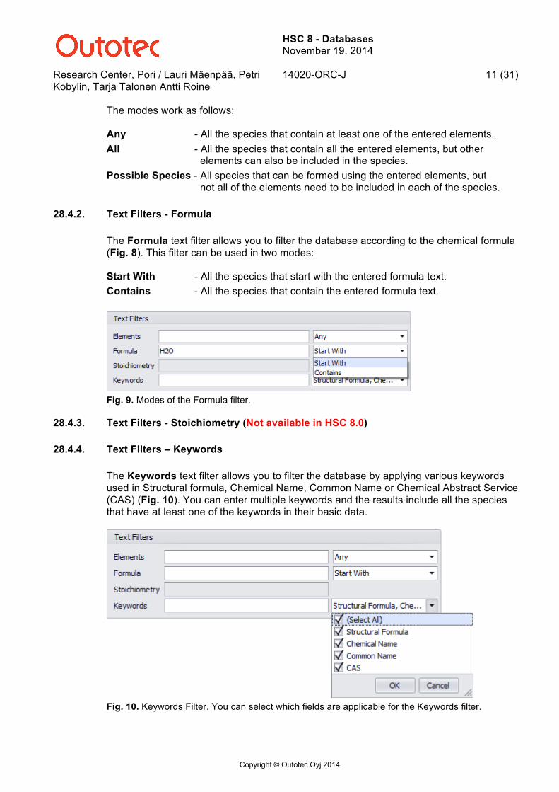
The Formula text filter allows you to filter the database according to the chemical formula (Fig. 8). This filter can be used in two modes: Start With - All the species that start with the entered formula text. Contains - All the species that contain the entered formula text.

Fig. 9. Modes of the Formula filter.

28.4.3. Text Filters - Stoichiometry (Not available in HSC 8.0)

28.4.4. Text Filters – Keywords The Keywords text filter allows you to filter the database by applying various keywords used in Structural formula, Chemical Name, Common Name or Chemical Abstract Service (CAS) (Fig. 10). You can enter multiple keywords and the results include all the species that have at least one of the keywords in their basic data.

Fig. 10. Keywords Filter. You can select which fields are applicable for the Keywords filter.



14020-ORC-J 12 (31)


28.4.5. Type Filters Type Filters can be used to filter out species that belong to certain phases (Fig. 11). These filters can also be used to exclude the electron and fluid species from the matching species.

Fig. 11. Type Filters. You can select which phases are included in the matching species list. You can also include or exclude the electron and fluid species.

28.4.6. Organic Filter Organic Filter is used to narrow down the list of matching species for organic compounds. If you do not want to see organic compounds in the matching species list, you can easily filter them out by un-checking the ‘Include Organics’ checkbox. This will exclude all the species which contain three or more carbon atoms in their chemical formula. You can also specify the amount of carbon atoms in the species that you wish to be included in the matching species list (Fig. 12).

Fig. 12. Organic Filter. You can specify the amount of carbon atoms in the species, by entering the values in the ‘Range of Carbon Atoms’ box.



14020-ORC-J 13 (31)


28.5. Diagrams You can plot the thermochemical data for a selected set of species by using the Diagrams options. In order to plot the data, you must first select the species for which you want the graphs to be drawn. Selection can be carried out in several ways. You can double click, drag and drop, or use the option in the right click menu to import the species to the Selected Species box (Fig. 13). Note that you can drag and drop multiple species simultaneously by holding down the Ctrl and Shift keys.

Fig. 13. Importing species to the Selected Species box.

Once you have the all the species in the Selected Species box, you can select the correct diagram type from the Diagrams options (Fig. 14).

Fig. 14. Select the thermochemical property to be plotted for the Selected Species.



14020-ORC-J 14 (31)


After selecting the correct property, HSC will automatically draw the diagram using HSC Diagrams (Fig. 15).

Fig. 15. HSC Diagrams can be used to plot thermochemical data for the species in the database.



14020-ORC-J 15 (31)


28.6. Editing data in the Own database HSC allows you to create your own database and edit its content. Editing is only available for the active Own database. To edit the data of a species in the Own database, first select the correct species and then activate the Edit mode from the top menu (Fig. 16); then you can change the data of the selected species (Fig. 17). Once you have edited the data, save the changes with the Save button at the top.

Fig. 16. Edit and View mode. Editing is possible only for the species in the Own database.

Fig. 17. Editing data in the Own database. Edited data can be saved with the Save button, and cancelled with the View button.

You can edit any value or text if you have more accurate data available, and you can also add or delete temperature ranges. To add a new species to your Own database, click Add New Species from the top menu (Fig. 18).



14020-ORC-J 16 (31)


Fig. 18. Adding new species to the Own database. You can also use existing Main database species as templates and add them to your Own database by right clicking the species in the Matching Species list and selecting Add to Own DB (Fig. 19). This will create a copy of that Main database species to the Own database, which can then be edited.

Fig. 19. Using Main database species as templates for Own database species.

28.6.1. Adding and removing temperature ranges You can add or remove temperature ranges in the Own database to extend or limit the valid temperature range of the species. In the edit mode, you can manipulate the data fields of the temperature ranges(Fig. 20). Note that when editing temperature ranges, you should pay attention to the enthalpy and entropy values in the first column and also make sure that the temperature range, as a whole, is continuous.

Fig. 20. Adding temperature ranges.

28.6.2. Commenting on data in the Own database

Commenting on data values is also possible in HSC 8.0. You can add a comment to a certain field by entering the Edit mode, selecting the field you want to comment on and clicking the Add/Remove Comment from the right click menu (Fig. 21). This will open a



14020-ORC-J 17 (31)


dialog in which you can enter or remove the comment (Fig. 22). Finally, you can see the added comments any time in the View mode, by clicking the commented field in the database (Fig. 23). Note that all the commented fields in the database are indicated by color-coding.

Fig. 21. Adding a comment to a value field. You can also add comments to the cells in the temperature range table.

Fig. 22. Enter the comment in the Comment dialog.

Fig. 23. Comments can be displayed in the database by clicking the commented fields in the View mode. Commented fields are presented using color-coding.

The cells in the spreadsheet can also be commented. In the Edit mode, right click the cell and select Insert Comment. This will open textbox for the comment (Fig. 24). Comments in the spreadsheet can be identified with red marker in the cell (Fig. 24).

Fig. 24. Commenting the cells in the spreadsheet.



14020-ORC-J 18 (31)


28.7. Data fields in HSC databases In HSC databases, data is given in two classes, Basic Data, and Temperature Ranges (Fig. 25). Basic Data contains general information about the species, such as the name and molecular weight, whereas Temperature Ranges contains temperature-dependent data. Each of the data fields is described in more detail in the following section.

28.7.1. Basic Data Formula

The formula must always be given. The valid formula syntax is described in section 28.2.1. The database editor will use this formula when it is calculating the molecular weight. The use of the correct state identifier (g, l, a, etc.) is extremely important, because the calculation modules handle the species in different ways. The state identifier “g)” must always be used for a gaseous species and “a)” for an aqueous species. Solid species can be given without the state identifier “s”. Liquid species and different structural forms can be specified in two ways: A. One formula for liquid and solid phases

This format is traditionally used for inorganic species, see the example in Fig. 25. Solid and liquid copper sulfides, as well as its different crystallographic forms, have the same formula, Cu2S, in the database. It is extremely important to note that: The enthalpy H value in the first temperature range must be the heat of the formation of solid Cu2S at 298.15 K and 1 bar. The entropy S value in the first temperature range must be the standard entropy of solid Cu2S at 298.15 K and 1 bar. The enthalpy H value in the following temperature ranges must be the heat of phase transformation at the phase transformation temperatures. The following phase transformations can be seen in Fig. 25:

- 376 K: Orthorombic α-Cu2S → hexagonal β-Cu2S

- 717 K: Hexagonal β-Cu2S → cubic γ-Cu2S

- 1402 K: Cubic γ-Cu2S → liquid Cu2S



14020-ORC-J 19 (31)


Fig. 25. Data of Cu2S species in the HSC Database.

The entropy S values in the following temperature ranges are the entropy changes in the phase transformations. Note that trSΔ can be calculated from the corresponding trHΔ

values using Equation (1) at the transition temperature trT . Bear in mind that this relation is not valid for the heat of formation and standard entropy values at 298.15 K.

tr

trtr T

HS Δ=Δ (1)

B. Different formulae for liquid and solid phases

The same data can also be given using different formulae for each species. The copper sulfide data in Fig. 25 may be divided into four separate phases: Cu2S(A), Cu2S(B), Cu2S(C) and Cu2S(l). It is, however, extremely important to note that for each phase: The H value in the first temperature range must always be the heat of formation of solid Cu2S(A), Cu2S(B), Cu2S(C) or liquid Cu2S(l) at 298.15 K and 1 bar. The S value in the first temperature range must always be the standard entropy of solid Cu2S(A), Cu2S(B), Cu2S(C) or liquid Cu2S(l) at 298.15 K and 1 bar, respectively. The enthalpy and entropy change values for phase transformations cannot be used. The heat of formation and standard entropy values for each state must be extrapolated from the normal stability range down to 298.15 K. Quite often the heat of formation and standard entropy values for organic species are given separately for gas, liquid and solid phases at 298.15 K. These values can easily be saved in the HSC database. However, different formulae must be used for each phase. See, for example, solid benzene C6H6(BZE), liquid C6H6(BZEl) and gaseous C6H6(BZEg) in the HSC Main Database.



14020-ORC-J 20 (31)


Structural Formula The structural formula is not utilized by the calculation modules, but it can be used to specify the species. It may also be used to save normal formula synonyms. Chemical Name The chemical name is not needed in thermochemical calculations, but it is very useful when selecting species for the calculations. Please use lower case characters, but start with an upper case character. Common Name Usually substances have a short common name that is used instead of the long chemical name. Mineralogical, trade, etc. names as well as synonyms can be used. Please try to use the most common ones in the HSC databases and use lower case characters, but start with an upper case character. Chemical Abstract Number The Chemical Abstract Number is one precise way to specify substances. However, this number is not usually available in the original references of the HSC database, therefore these data are partly missing in HSC 8.0. However, this data field gives the users the possibility to use CAS numbers in the Own database. Molecular Weight The molecular weight is calculated automatically in HSC 8.0. The calculation is based on the chemical formula of the species, written in the Formula field. Melting and Boiling points These data are not used by the calculation modules. However, the values are very helpful when analyzing the calculation results. Negative values mean that the substance decomposes before the melting or boiling point. H° formation at 298.15 K This field shows the formation enthalpy of the species at 298.15 K. The value for this field is read from the first range of the Temperature Ranges table. S° at 298.15 K This field shows the absolute entropy of the species at 298.15 K. The value for this field is read from the first range of the Temperature Ranges table. Cp° at 298.15 K This field shows the heat capacity of the species at 298.15 K. The value for this field is calculated from the appropriate temperature range of the Temperature Ranges table.



14020-ORC-J 21 (31)


28.7.2. Temperature Ranges Temperature Range (Tmin and Tmax) A valid temperature range must always be given for the H, S, and Cp data, because the calculation modules use these temperatures in nearly all calculations. The basic idea of the temperature ranges is described in the previous Formula section. Remember also that: - The first limit, Tmin, is the lowest temperature where the Cp coefficients A, B, C, and

D are valid. Traditionally, the first temperature range starts from 298.15 K (= Tmin). However, other temperatures may also be used.

- The second temperature, Tmax, is the highest temperature where the Cp coefficients A, B, C, and D are valid.

- Quite often the upper limit, Tmax, is the phase transformation temperature. However, sometimes the heat capacity temperature dependence of a phase is so complicated that it has been divided into several ranges. In these cases, the phase transformation enthalpy and entropy values are zero (0).

- The temperature ranges of a substance and formula must be continuous. No discontinuities are allowed.

Phase The correct state must be given for the species: g for gases, l for liquids, s for solids and a for aqueous. H

The first enthalpy value at 298.15 K and 1 bar must always be the heat of formation of the same state as that described in the formula and phase fields. If there are several temperature ranges, the other H values are the heat of transformation at the phase transformation temperatures. Note that the heat of formation for elements is zero at 298.15 K. S

The first entropy value at 298.15 K and 1 bar must always be the standard entropy of the same state as that described in the formula and phase fields. If there are several temperature ranges, the other S values are the entropies of phase transformations at the transformation temperatures. Cp coefficients A, B, C and D

These values are the coefficients of the heat capacity function, see the equation in the header of the Temperature Ranges table or Chapter 8. Introduction, Equation (4). These coefficients are not needed if thermochemical calculations are done at 298.15 K or near that temperature. At other temperatures, it is essential to know these data. Quite often the A, B, C, and D coefficients are not available, and the heat capacity values are listed as a function of temperature only. These values can easily be converted to A, B, C, and D coefficients using the Fit Cp Data (28.10 Fitting Cp data) option of the database menu. Sometimes the coefficients A, B, C, and D are given for other heat capacity functions than those used in HSC Chemistry. Their coefficients can also be converted to HSC format using the Fit Cp Data option of the database menu.



14020-ORC-J 22 (31)


Density

The calculation modules use density values in the mol - kg - Nm3 - conversions. However, missing density values do not usually cause too much trouble. Kg/l units have been used for condensed species and g/l for gases. Color The color of a species is given as a numver. You can find the available color options from section 28.14. Database Appendix A: Color codes. Solubility

These values are available for some species, but they are not used in calculations in HSC 8. This field is provided in order to guarantee the compatibility of the database with future versions of HSC. Reference

It is always recommended to give the original reference of the data. Most of the references used are cited with abbreviations. The abbreviations are formed using the author name and the year of publication. The Main database abbreviations are given in alphabetical order in Chapter 32. Data references. Reliability Class The data in the HSC Main database have been collected from a large number of sources. Especially in some old sources, the accuracy of the H, S, and Cp data does not seem to be so good. However, all of these data have been included in the Main database, because in some cases small errors in the basic thermochemical data are not critical. The reliability class gives a rough estimate of the reliability of the data. The best reliability code is 1 and worst is 10. Usually, new data books have a reliability class of 1. The user can easily edit the reliability class in the same way as the rest of the cells.



14020-ORC-J 23 (31)


28.8. Fitting Cp data Quite often only the heat capacity values at different temperatures are available. You can convert these data to A, B, C, and D coefficients using the Fit Cp Data tool (Fig. 26 and Fig. 27) and by following these steps:

Fig. 26. Fit Cp Data tool.

Fig. 27. HSC database Cp Fitting module.

1. Select Edit mode and click Fit Cp Data (Fig. 26). 2. Type the temperature and the experimental heat capacity values to the table on the

left in Fig. 27. Make sure that the entered data has the "J/(mol*K)" units. 3. Add the appropriate Tmin(K) and Tmax(K) values for each temperature range which

you want to fit in the Fitted Data table. Note that the total temperature range has to be continuous.

4. Click Fit Cp to get the A, B, C, and D coefficients for each of the ranges. To fit each range, you need to select a cell in the correct temperature range column and click the Fit Cp button.

5. You can evaluate the results of the fitted data by comparing the plots of the experimental and the fitted Cp in the graph. Also, you can find the error value of each of the temperature ranges in the fitted data table.



14020-ORC-J 24 (31)


6. If the first fitting fails to produce acceptable results, try dividing the temperature ranges differently or adding more ranges to get a better fit. You can also try to get better results by forcing the fitting to disregard certain coefficients for certain ranges. To do this, type "N" in the coefficient cell, which you want to be disregarded in the fitting.

7. You can also try to input the coefficients manually and reproduce the fitted curve by clicking Calculate Cp.

8. You can estimate the Cp values for the species with Estimate Cp. The Estimation function uses the species name as a parameter and you can also give additional parameters for the estimation with the Species Type and Structure lists.

9. When all the ranges have been fitted, you can copy the coefficients to the database by pressing Update Species. Note that the edited data has to be saved in the Own database file using the options in the Editor's File menu.

28.8.1. Converting Cp functions

In some references, the Cp coefficients A, B, C, D, etc. are based on another Cp expression than that used in HSC Chemistry. The coefficients cannot be saved in the HSC databases as such, but they can be converted to HSC format using the Import from Equation tool (Fig. 28).

Fig. 28. Converting Cp functions to HSC format (Import from Equation).



14020-ORC-J 25 (31)


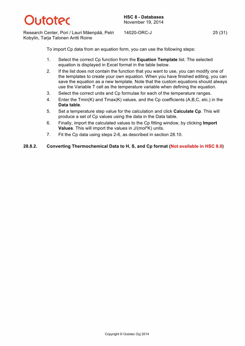
To import Cp data from an equation form, you can use the following steps: 1. Select the correct Cp function from the Equation Template list. The selected

equation is displayed in Excel format in the table below. 2. If the list does not contain the function that you want to use, you can modify one of

the templates to create your own equation. When you have finished editing, you can save the equation as a new template. Note that the custom equations should always use the Variable T cell as the temperature variable when defining the equation.

3. Select the correct units and Cp formulae for each of the temperature ranges. 4. Enter the Tmin(K) and Tmax(K) values, and the Cp coefficients (A,B,C, etc.) in the

Data table. 5. Set a temperature step value for the calculation and click Calculate Cp. This will

produce a set of Cp values using the data in the Data table. 6. Finally, import the calculated values to the Cp fitting window, by clicking Import

Values. This will import the values in J/(mol*K) units. 7. Fit the Cp data using steps 2-6, as described in section 28.10.

28.8.2. Converting Thermochemical Data to H, S, and Cp format (Not available in HSC 8.0)



14020-ORC-J 26 (31)


28.9. Combining Database files If you have several Own databases and you wish to combine them into a single database, you can use the Database Merge tool (Fig. 29 and Fig. 30). The merging of database files creates a new file without deleting the original files.

Fig. 29. Database combining tool.

Fig. 30. Combining two HSC database files.

Please follow these steps to combine any two HSC databases: 1. Load the two databases to be combined using the First File and Second File

buttons. 2. Click Start at the top right of the window to obtain the species from both files in the

Species list. 3. The Species list presents the species from both databases with the following color-

coding: Valid These are the species which will be included in the new database file. Species

that are identical in both databases are initially marked Valid. You can mark other species Valid by right clicking the species name and selecting Add Item.

Missing These species are found in the first file, but not in the second file.

Added These species are found in the second file, but not in the first file.

Modified These species are found in both databases (First File and Second File), but there are differences in the data. The values that are different are highlighted.



14020-ORC-J 27 (31)


4. Choose the species that you want to include in the new database and add them as "Valid".

5. Save the new database by clicking Save File. Note that you can also edit and comment on the species data in the merging dialog before saving the file.

28.9.1. Database combining example

Start the combining by selecting two databases (Fig. 31) and click Start.

Fig. 31. Select the two databases

Once the databases are loaded, the species are automatically color-coded (Fig. 32).

Fig. 32. Color-coded species.

The results in the Fig. 32 show that the two databases contain: one species which is identical in both databases (Valid), four species which can be found only in the first selected database (Missing), four species which can be found only in the second database (Added) and two pairs of species which can be found from both databases, but the data is different (Modified - First File and Modified - Second File).



14020-ORC-J 28 (31)


The next step in combining the databases is to select the species which are to be included in the merged database. The status for the included species needs to be Valid. For example, to include the species which were present only in either of the databases can be easily changed as valid by, applying the species filters, and clicking Add Item for the selected species (Fig. 33 and Fig. 34).

Fig. 33. Change species status to Valid by clicking Add Item.

Fig. 34. The included species appear as Valid.

Usually the last thing to check is the species that exists in both selected databases. These species appear as pairs and they have the Modified status. The first of the modified species pair is always from the "First File" database and the second species from the "Second File" database. The differing data values in these species are indicated with red font color. You can choose to include none, either one or both of the species. If both of the modified species are selected, then the formula of the latter species will be identified with an added index number. When the statuses of all the species, to be included in the new database, are changed to valid, the combined database can be saved by clicking Save File.



14020-ORC-J 29 (31)


28.10. Selecting active database Two databases can be open at the same time. They are called Own and Main. Almost any valid file name and directory can be used. However, the suffix (type) of these files must be *.xml. Old *.HSC files can be imported to the database and saved in the new format. (Note: Awdb4.HSC file is in HSC internal use). HSC Chemistry calculation modules primarily use the data in the Own database. If a species is not found in the Own database, HSC tries to find it in the Main database. You can check the currently used active databases from the menu at the bottom of Database Editor (Fig. 35).

Fig. 35. Active databases in HSC 8.

Active databases can be changed at any time from the File menu at the top (Fig. 36). The active databases can be selected using Load Own Database and Load Main Database.

Fig. 36. Changing the active databases.



14020-ORC-J 30 (31)


28.11. Database Browser Many of the modules in HSC can call the Database Browser to check data and also to import species to the modules. The browser contains the same filtering options as the editor, but editing the data is disabled in the browser. Another difference between the browser and the editor is the tool for importing species to certain modules (Fig. 37).

Fig. 37. HSC Database Browser.

To import a species from the database to the modules, first you need to add the correct species to the Selected Species box (see section 28.6. Diagrams). Once you have selected all the species, click Import Items to import the species to the module (Fig. 38).

Fig. 38. Import selected species to the module.



14020-ORC-J 31 (31)


28.12. Database Appendix A: Color codes The color of the substances is given for some species with the following color codes in HSC 8.0 Main database:

0. No data available

1. Blue

2. Green

3. Cyan

4. Red

5. Magenta (blue-red)

6. Brown

7. White

8. Dark Gray

9. Light Blue

10. Light Green

11. Light Cyan

12. Light Red

13. Light Magenta

14. Light Yellow

15. Bright White

16. Colorless

17. Yellow

18. Gray

19. Black

20. Orange

21. Yellow-gray

22. Yellow-brown

23. Red-brown

24. Orange-yellow

25. Yellow-green

26. Black-brown

27. White brown

28. Orange-green

29. Blue-green

30. Dark Green

31. Blue-black

32. Red-orange

33. Yellow-orange

34. Green-yellow

35. Brown-black

36. Green-blue

37. Orange-red

38. Brown-yellow

39. Dark Red

40. Brown-violet

41. Red-violet

42. Violet-black

43. Yellow-black

44. Blue-white

45. Red-black

46. Green-black

47. Purple-black

48. Gray-brown

49. Brown-red

50. Gold-brown

51. Gold-yellow

52. Blue-gray

53. Orange-brown