Dissertation

2D-3D Registration of Vascular ImagesTowards 3D-Guided Catheter Interventions

Martin Groher

Computer Aided Medical Procedures(CAMP)

Prof.Dr. Nassir Navab

Fakultät für InformatikTechnische Universität München

Technische Universitat Munchen, Fakultat fur InformatikComputer-Aided Medical Procedures & Augmented Reality

2D-3D Registration of Vascular ImagesTowards 3D-Guided Catheter Interventions

Martin Groher

Vollstandiger Abdruck der von der Fakultat fur Informatik der TechnischenUniversitat Munchen zur Erlangung des akademischen Grades eines

Doktors der Naturwissenschaften (Dr. rer. nat.)

genehmigten Dissertation.

Vorsitzender: Univ. Prof. Dr. Bernd Radig

Prufer der Dissertation:

1. Univ. Prof. Nassir Navab, PhD

2. Prof. Dr. ir. Max A. Viergever,

University Medical Center Utrecht/Niederlande

Die Dissertation wurde am 20.09.2007 bei der Technischen Universitat Muncheneingereicht und durch die Fakultat fur Informatik am 18.03.2008 angenommen.

iii

Abstract

Angiographic imaging is a widely used monitoring tool for minimally invasivevascular treatment and pathology access. Especially in deforming abdominal areas,the registration of pre- and intraoperative image data is still an unsolved problem,but important in several aspects. In particular, treatment time and radiation expo-sure to patient and physician can be significantly reduced with the resulting 2D-3Ddata fusion.

The focus of this work is to provide methods for the registration of 2D vascularimages acquired by a stationary C-arm to preoperative 3D angiographic ComputedTomography (CT) volumes, in order to improve the workflow of catheterized livertumor treatments.

Fast and robust vessel segmentation techniques are used to prepare the necessarygraph data structures for a successful alignment. Here, we introduce restricted cor-respondence selection and iterative feature space correction to drive the proposedrigid-body algorithms to global and accurate solutions. Moreover, it is shown for thefirst time that the assignment of natural constraints on vessel structures allows for asuccessful recovery of a 3D non-rigid transformation despite a single-view scenario.

Based on these results, novel volumetric visualization and roadmapping tech-niques are developed in order to resolve interventional problems of reduced depthperception, blind navigation, and motion blur.

Keywords:2D-3D Registration of Medical Images, Segmentation of Vascular Structures, Angiog-raphy

iv

Zusammenfassung

Angiographische Bildgebung ist ein weitverbreitetes Verfahren zur Uberwachungminimal-invasiver Gefaßbehandlungen. Vor allem in deformierbaren Bereichen desAbdomens stellt die Registrierung von pra- und intraoperativen Bilddaten noch im-mer ein ungelostes Problem dar. Sie birgt jedoch einen großen Zugewinn, da durchdie daraus resultierende Bildfusion insbesondere die Behandlungszeit und die Strah-lungsbelastung sowohl fur den Patienten als auch fur den behandelnden Arzt redu-ziert werden konnen.

Der Fokus dieser Arbeit liegt auf der Entwicklung von Methoden zur Registrie-rung von 2D Vaskularbildern, die mittels eines stationaren C-Bogens aufgenommenwerden, zu praoperativen 3D CT Angiographievolumen. Dadurch soll der Arbeits-ablauf von Kathetereingriffen zur Behandlung von Lebertumoren verbessert wer-den.

Schnelle und robuste Gefaßsegmentierungstechniken werden angewandt, um diezur Registrierung notwendigen Graphenstrukturen vorzubereiten. Eine restriktiveKorrespondenzauswahl sowie iterative Korrekturen eines Merkmalsraumes werdenvorgestellt. Diese Techniken sind notwendig, um die in dieser Arbeit entwickelten ri-giden Registrieralgorithmen zu globalen und akkuraten Losungen konvergieren zulassen. Daruber hinaus wird gezeigt, dass eine nichtrigide 3D Transformation unterder Verwendung nur eines einzelnen Blickwinkels berechnet werden kann, indemnaturliche Beschrankungen auf die Bewegung von Gefaßen mathematisch formu-liert und eingesetzt werden.

Basierend auf diesen Registrierungsergebnissen werden neue volumetrische Vi-sualisierungsverfahren sowie “Roadmapping” Techniken entwickelt, um Interventi-onsprobleme wie verminderte Tiefenwahrnehmung, blinde Katheternavigation, undBewegunsverzeichnungen zu losen.

Schlagworter:2D-3D Bildregistrierung, Segmentierung von Vaskularsystemen, Angiographie

v

Acknowledgments

First of all, I’d like to thank Professor Nassir Navab for the extraordinary supervi-sion I received. Additional Saturday meetings in coffee shops, or nightly discussionsvia Skype are most probably not very common among doctor fathers - a privilege Iappreciated very much.

I’d also like to thank all the people from CAMP, which (some more, some less)helped me achieve my research goals. In particular, I want to thank Andreas Keilfor enduring my numerous attempts to discuss scale-spaces, filtering, or transforma-tions, and Ben Glocker for proof-reading and the various discussions on balconies,or in pubs, which started with work but mostly ended somewhere totally different.I want to thank Darko Zikic for the most careful proof-reading, the ideas he shared,and the great time we had in our common office. Thanks to Pierre who visited me inthe mornings even though I have the most remote office of all, and to Martin Hornfor pimping all the multimedia. Also, I want to thank all the students that helpedme during the time of my PhD work, especially Nicolas Padoy and Frederik Bender.I am also grateful for all the help and valuable explanations I got from my physicianpartners, in particular Tobias Jakobs, Ralf Hoffmann, and Tobias Waggershauser. Ofcourse, thanks to Siemens AX for their financial support, and to Klaus Klingenbeck-Regn as well as Marcus Pfister for valuable input.

I’m very much obliged to my parents, who always supported me during my stud-ies, and made this thesis possible in the first place. Their understanding and supportwas exceptional and priceless. I’m indebted to my sister Evi, who always knew howto motivate me, either by choosing the right words, or the right mountain to climb,or by simply sharing the same situation. Finally, I want to say thank you to Simone,who accompanied me during this (sometimes happy, sometimes troublesome) time.Thank you, Simone, for being with me during all the minor and major crisis that Ifaced in the last three years, thank you for encouraging me, cheering me up, andpreventing me of loosing focus. Without any of you four this thesis would not havehappened.

Contents

Brief Summary of the Thesis xi

Outline of the Thesis xiii

I. Introduction, Methodology, and State of the Art 1

1. Introduction 31.1. Problem Statement . . . . . . . . . . . . . . . . . . . . . . . . . . . . . . 4

1.1.1. Terminology . . . . . . . . . . . . . . . . . . . . . . . . . . . . . . 51.2. Angiography in the Clinic . . . . . . . . . . . . . . . . . . . . . . . . . . 7

1.2.1. Preoperative Imaging: CTA and MRA . . . . . . . . . . . . . . . 71.2.2. Intraoperative Imaging: C-arms . . . . . . . . . . . . . . . . . . 8

1.3. A Registration System for Abdominal Catheterizations . . . . . . . . . 101.3.1. Imaging for Liver Interventions . . . . . . . . . . . . . . . . . . . 111.3.2. Justification for a 2D-3D Angiographic Registration . . . . . . . 111.3.3. Medical and Technical Requirements . . . . . . . . . . . . . . . 12

1.4. Contribution . . . . . . . . . . . . . . . . . . . . . . . . . . . . . . . . . . 13

2. Methodology 152.1. Images . . . . . . . . . . . . . . . . . . . . . . . . . . . . . . . . . . . . . 152.2. Vessels in Medical Images . . . . . . . . . . . . . . . . . . . . . . . . . . 17

2.2.1. The Hessian in Vessel Analysis . . . . . . . . . . . . . . . . . . . 172.2.2. Vessel Enhancement . . . . . . . . . . . . . . . . . . . . . . . . . 192.2.3. Segmentation Initialization . . . . . . . . . . . . . . . . . . . . . 202.2.4. Segmentation . . . . . . . . . . . . . . . . . . . . . . . . . . . . . 212.2.5. Quantification . . . . . . . . . . . . . . . . . . . . . . . . . . . . . 222.2.6. Suggestions for Method Selection . . . . . . . . . . . . . . . . . 26

2.3. Medical Image Registration . . . . . . . . . . . . . . . . . . . . . . . . . 272.3.1. Data Terms . . . . . . . . . . . . . . . . . . . . . . . . . . . . . . 282.3.2. Transformations . . . . . . . . . . . . . . . . . . . . . . . . . . . 302.3.3. Correspondences . . . . . . . . . . . . . . . . . . . . . . . . . . . 342.3.4. Optimization . . . . . . . . . . . . . . . . . . . . . . . . . . . . . 36

2.4. 2D-3D Registration . . . . . . . . . . . . . . . . . . . . . . . . . . . . . . 382.4.1. Rigid 2D-3D Registration . . . . . . . . . . . . . . . . . . . . . . 392.4.2. Calibration . . . . . . . . . . . . . . . . . . . . . . . . . . . . . . . 402.4.3. Error Analysis . . . . . . . . . . . . . . . . . . . . . . . . . . . . . 41

3. State of the Art in 2D-3D Angiographic Registration 45

viii Contents

3.1. Intensity-based 2D-3D Registration . . . . . . . . . . . . . . . . . . . . . 453.1.1. DRR Generation . . . . . . . . . . . . . . . . . . . . . . . . . . . 463.1.2. Registration Algorithms . . . . . . . . . . . . . . . . . . . . . . . 48

3.2. Feature-based 2D-3D Registration . . . . . . . . . . . . . . . . . . . . . 503.2.1. Distance Functions . . . . . . . . . . . . . . . . . . . . . . . . . . 513.2.2. Optimizer-based Algorithms . . . . . . . . . . . . . . . . . . . . 523.2.3. ICP-based Algorithms . . . . . . . . . . . . . . . . . . . . . . . . 53

3.3. Hybrid 2D-3D Registration . . . . . . . . . . . . . . . . . . . . . . . . . 553.4. Deformable 2D-3D Registration . . . . . . . . . . . . . . . . . . . . . . . 573.5. Discussion . . . . . . . . . . . . . . . . . . . . . . . . . . . . . . . . . . . 58

3.5.1. Initialization . . . . . . . . . . . . . . . . . . . . . . . . . . . . . . 583.5.2. Directions of Future Research . . . . . . . . . . . . . . . . . . . . 59

II. New Algorithms for 2D-3D Angiographic Registration 61

4. Clinical Application 634.1. Medical Excursion: Liver Vessel Systems . . . . . . . . . . . . . . . . . 634.2. Treatment of Liver Tumors . . . . . . . . . . . . . . . . . . . . . . . . . . 644.3. Workflow of Transarterial Chemoembolizations . . . . . . . . . . . . . 664.4. Feasibility of 2D-3D Registration . . . . . . . . . . . . . . . . . . . . . . 67

4.4.1. Data Availability . . . . . . . . . . . . . . . . . . . . . . . . . . . 674.4.2. Challenges . . . . . . . . . . . . . . . . . . . . . . . . . . . . . . . 684.4.3. State-of-the-Art Applicability to TACE . . . . . . . . . . . . . . . 69

5. Rigid 2D-3D Registration of Angiographic Images 715.1. C-arm Model . . . . . . . . . . . . . . . . . . . . . . . . . . . . . . . . . . 715.2. Preprocessing . . . . . . . . . . . . . . . . . . . . . . . . . . . . . . . . . 73

5.2.1. Segmentation . . . . . . . . . . . . . . . . . . . . . . . . . . . . . 735.2.2. Extraction of Graphs . . . . . . . . . . . . . . . . . . . . . . . . . 735.2.3. Graph Representation of Vessel Centerlines . . . . . . . . . . . . 75

5.3. Bifurcation-Driven 2D-3D Registration . . . . . . . . . . . . . . . . . . . 765.3.1. Initialization . . . . . . . . . . . . . . . . . . . . . . . . . . . . . . 765.3.2. 4 DOF Optimization . . . . . . . . . . . . . . . . . . . . . . . . . 775.3.3. Algorithm Evaluation . . . . . . . . . . . . . . . . . . . . . . . . 795.3.4. Discussion . . . . . . . . . . . . . . . . . . . . . . . . . . . . . . . 81

5.4. Segmentation-Driven 2D-3D Registration . . . . . . . . . . . . . . . . . 825.4.1. MLE with Labelmaps . . . . . . . . . . . . . . . . . . . . . . . . 835.4.2. The EBM Algorithm for Angiographic Registration . . . . . . . . 855.4.3. Algorithm Evaluation . . . . . . . . . . . . . . . . . . . . . . . . 885.4.4. Discussion . . . . . . . . . . . . . . . . . . . . . . . . . . . . . . . 93

6. Deformable 2D-3D Registration of Angiographic Images 956.1. Method . . . . . . . . . . . . . . . . . . . . . . . . . . . . . . . . . . . . . 97

6.1.1. Setting and Preprocessing . . . . . . . . . . . . . . . . . . . . . . 97

Contents ix

6.1.2. Preliminaries and Notation . . . . . . . . . . . . . . . . . . . . . 986.1.3. The Model . . . . . . . . . . . . . . . . . . . . . . . . . . . . . . . 996.1.4. Difference Measure . . . . . . . . . . . . . . . . . . . . . . . . . . 1006.1.5. Length Preservation Constraint . . . . . . . . . . . . . . . . . . . 1006.1.6. Diffusion Regularization and Bending Energy . . . . . . . . . . 1016.1.7. Position Retention Constraint . . . . . . . . . . . . . . . . . . . . 1026.1.8. Optimization Scheme . . . . . . . . . . . . . . . . . . . . . . . . 102

6.2. Results and Evaluation . . . . . . . . . . . . . . . . . . . . . . . . . . . . 1036.2.1. Parameter Values and Smoothness Term . . . . . . . . . . . . . 1036.2.2. Tests on Synthetic Data . . . . . . . . . . . . . . . . . . . . . . . 1046.2.3. Real Data with Artificial Deformation . . . . . . . . . . . . . . . 1046.2.4. Real Data with Natural Deformation . . . . . . . . . . . . . . . . 1056.2.5. Clinical Test . . . . . . . . . . . . . . . . . . . . . . . . . . . . . . 105

6.3. Discussion . . . . . . . . . . . . . . . . . . . . . . . . . . . . . . . . . . . 107

7. Conclusion 1117.1. Workflow Integration . . . . . . . . . . . . . . . . . . . . . . . . . . . . . 112

7.1.1. Intraoperative Visualization . . . . . . . . . . . . . . . . . . . . . 1127.1.2. Real-Time Breathing Correction . . . . . . . . . . . . . . . . . . . 115

7.2. Future Work . . . . . . . . . . . . . . . . . . . . . . . . . . . . . . . . . . 116

Appendix 121

A. Practical Considerations on Images 121A.1. Image Filtering . . . . . . . . . . . . . . . . . . . . . . . . . . . . . . . . 121A.2. Image Derivatives . . . . . . . . . . . . . . . . . . . . . . . . . . . . . . . 122A.3. Linear Scale-Space . . . . . . . . . . . . . . . . . . . . . . . . . . . . . . 122

B. Thin Plate Splines 125B.1. Special Spline Smoothing Problem . . . . . . . . . . . . . . . . . . . . . 125B.2. Numerical Solution . . . . . . . . . . . . . . . . . . . . . . . . . . . . . . 126B.3. TPS for Feature-Based Deformable Registration . . . . . . . . . . . . . . 127

C. Rotation Parameterization 129C.1. Euler Angles . . . . . . . . . . . . . . . . . . . . . . . . . . . . . . . . . . 129C.2. Gimbal Lock . . . . . . . . . . . . . . . . . . . . . . . . . . . . . . . . . . 129C.3. Euler Angles in Rigid Registration . . . . . . . . . . . . . . . . . . . . . 130

D. Real-Time Respiratory Motion Tracking 131D.1. Method . . . . . . . . . . . . . . . . . . . . . . . . . . . . . . . . . . . . . 131

D.1.1. Motion Model . . . . . . . . . . . . . . . . . . . . . . . . . . . . . 131D.1.2. Approximation of Vessel Motion by Catheter Motion . . . . . . 131D.1.3. Motion Tracking on Enhanced Images . . . . . . . . . . . . . . . 132D.1.4. Dynamic Template Update . . . . . . . . . . . . . . . . . . . . . 132

D.2. Results . . . . . . . . . . . . . . . . . . . . . . . . . . . . . . . . . . . . . 133

x Contents

D.2.1. Simulation Studies . . . . . . . . . . . . . . . . . . . . . . . . . . 133D.2.2. Patient Studies . . . . . . . . . . . . . . . . . . . . . . . . . . . . 133

E. List of Symbols 137

F. List of Abbreviations 141

G. List of Publications 145

Bibliography 147

Brief Summary of the Thesis

In this thesis, we develop novel methods for the registration of angiographic 3D and2D data sets. We focus on liver catheterizations, in particular Transarterial Chemo-embolizations (TACE) as a frequently used treatment for liver tumors, where a fusionof preoperative CTA and intraoperative DSA data can provide valuable informationin terms of depth perception and intraoperative navigation, but also has to meetcertain requirements for automation, speed, and accuracy. The contributions of thiswork are the proposal of a new CTA protocol for artery visualization in a TACEworkflow, two novel rigid registration algorithms, and a method for deformable 2D-3D registration in a single-view scenario.

The introduction of a new CTA protocol to visualize liver arteries allows for afeature-based alignment, where the difficulties of vessel extraction, the correspon-dence problem in heterogeneous feature spaces, and non-rigid registration in a one-view scenario have to be overcome.

We will conceive two novel rigid registration algorithms, which were tailored to berobust against segmentation errors, different contrast propagation, and deformationchanges.

The bifurcation-driven registration restricts the feature space to ramification pointsof the underlying vessel structure and reduces the number of outliers by iterativegraph extraction on projected centerline images. By combining this technique withtopological information of the vessel graphs, a new distance function is developed.

While the bifurcation-driven registration yields good results in many clinical cases,it also requires a minimal amount of user interaction intraoperatively. Thus, we de-velop a second technique that performs fully automatic during the intervention. Thesegmentation-driven registration combines 2D DSA segmentation with 2D-3D pose es-timation using a probability map in order to consequently discard false positives inthe two vascular systems. This probability link, embedded in a Maximum Likeli-hood formulation, proves to be beneficial in terms of accuracy (ca. 1.45 mm meanProjection Distance (mPD)) and robustness compared to hybrid methods, whichavoid 2D segmentation. Since this enhanced feature space does not require an opti-mal segmentation, an automatic seed detection can be employed to provide an inte-gration into intraoperative workflow without additional user interaction.

Both algorithms are evaluated on simulated as well as several clinical data sets,root mean square errors and target registration errors are measured, and MonteCarlo simulations are carried out to show the high accuracy and robustness of theproposed methods despite non-rigid motion.

A further issue that is addressed in this thesis is the refinement of a (sub-optimal)rigid vascular alignment in a non-rigid environment. A new 2D-3D deformable reg-istration algorithm is proposed that solves for a 3D deformation field using only theinformation of a single view. The minimization of an energy term based on the Eu-

xii Contents

clidean distance between corresponding points is rendered well-posed by incorpo-rating natural and mathematically valid constraints of length preservation of vesselstructures and smoothness of local transformations. A 3D deformation field can becomputed thus, where even the displacement in projection direction is captured, im-proving the results of rigid 2D-3D registration considerably.

The integration of the computed results into interventional workflow will be ad-dressed in the end of the work. Proper visualization techniques are developed toproject roadmap information onto the current 2D image, or to visualize 2D catheterlocations in 3D via correspondence information. After DSA acquisition, cliniciansusually continue the navigation by means of fluoroscopic imaging. Tracking the ap-parent motion of the catheter in 2D allows for a propagation of the registration resultsto these subsequent images. Thus, registration results can be updated to the currentclinical situation and intraoperative 3D visualization is not hampered by breathingmotion.

Outline of the Thesis

This thesis is subdivided into two parts.The first part provides an introduction, the methodological background, and a re-view of existing techniques.The second part presents details on the clinical applications, new algorithms for 2D-3D registration, and a conclusion section with extensions and future work.

Part I: Introduction, Methodology, and Review

CHAPTER 1: INTRODUCTION

A general introduction into the problem, a description of angiographic devices usedin medical imaging, and a justification for a 2D-3D registration system for angio-graphic treatments.

CHAPTER 2: METHODOLOGY

The methodological basis of this thesis, including vessel analysis, issues for medicalimage registration, and a focus on 2D-3D registration in a C-arm scenario.

CHAPTER 3: STATE OF THE ART IN 2D-3D ANGIOGRAPHIC REGISTRATION

A review of existing techniques for 2D-3D vascular image registration.

Part II: New Algorithms for 2D-3D Angiographic Registration

CHAPTER 4: CLINICAL APPLICATION

The clinical application that is focused in this work, Transarterial Chemoembolization.A short introduction in liver vessel systems and tumor treatment followed by a crit-ical analysis in terms of challenges and applicability of state-of-the-art algorithms.

CHAPTER 5: RIGID 2D-3D REGISTRATION OF ANGIOGRAPHIC IMAGES

Two new algorithms for rigid 2D-3D registration. A one-click technique for regis-tration based on bifurcation alignment aided by topological information, and a fullyautomatic method based on iterative segmentation and alignment using vessel prob-abilities.

CHAPTER 6: DEFORMABLE 2D-3D REGISTRATION OF ANGIOGRAPHIC IMAGES

xiv Contents

A novel method for 2D-3D deformable registration of a vascular model to a singleprojection image.

CHAPTER 7: CONCLUSION

A short summary followed by a discussion of the integration of the registration al-gorithms into clinical workflow and future work.

Appendix

PRACTICAL CONSIDERATIONS ON IMAGES

Some implementation details for image analysis.

THIN PLATE SPLINES

A deformation model used for the deformable registration algorithm derived in thethesis.

ROTATION PARAMETERIZATION

A short summary of the chosen parameterization for 3D rotations.

REAL-TIME RESPIRATORY MOTION TRACKING

An algorithm for tracking and compensation of breathing motion apparent in fluo-roscopic image sequences.

LIST OF SYMBOLS

The mathematical symbols used.

LIST OF ABBREVIATIONS

A list of abbreviations used throughout the work.

LIST OF PUBLICATIONS

All publications contributed to the scientific community during this work.

Part I.

Introduction, Methodology,and State of the Art

1. Introduction

Angiographic interventions or surgeries are performed on an every-day basis inmany hospitals. Blood vessels, distributed throughout the body, have to be accessedfor numerous medical procedures such as stenting of coronary arteries, treatmentof stenoses in brain vessels, reduction of blood pressure, or embolization of tumorvessels to name a few. Nowadays, such treatments can be guided by angiographicimaging, supporting physicians in the assessment of instrument and blood vessellocations. In contrast to open surgery, treatments guided by angiographic imagescan be performed minimally-invasive, i.e. only a small incision is needed to injectinstruments, which can be located and navigated by the use of the acquired images.

It is common in hospitals that images of patients are acquired before the treat-ment (preoperatively) for diagnosis and/or for procedure planning. These preoper-ative images are usually of high quality and are acquired in 3D (e.g. using MagneticResonance (MR) or Computed Tomography (CT) scanners). Imaging data acquiredduring medical procedures are of less quality, which means in this respect that theyusually have a lower signal-to-noise ratio (SNR), and a lower dimensionality (2Dslices or 2D projections instead of full 3D volumes). They usually have, however,a higher spatial resolution, which is due to the high zooming capabilities of intra-operative imaging devices. This intraoperative data is used to assess the state ofinstruments and patient anatomy over time. Even though recent advances in in-traoperative imaging have brought 3D acquisitions into operating rooms (e.g. 3Drotational angiography) yielding nearly the same quality as preoperative scanners,they are - due to hard time constraints and high X-ray dosage - performed seldomly.Moreover, they do not capture the temporal aspect of the procedure, i.e. advance-ments of instruments or changes of anatomy due to deformation cannot be assessedby a static 3D scan.

The registration of pre- and intraoperative data sets would fuse patient anatomyinformation of superior quality with information capturing the current state of theoperation. With this registration, new ways of intraoperative roadmapping and nav-igation can be introduced, the treatment can be sped up, and harmful radiation thatphysicians and patients are exposed to can be reduced. Such registration systems arealready commercially available for surgery procedures, however, no angiographicregistration system has been launched on the market yet. This is due to the difficultyto directly apply existing techniques (often based on external tracking) to vascula-ture deformed by internal organ movement. However, especially in deformable re-gions like thoracic or abdominal areas, the task of vascular image alignment, whilechallenging from a technical point of view, yields the maximal benefit for the operat-ing physician, since navigating a catheter through moving structures requires a highlevel of dexterity, training, and anatomical knowledge.

Since angiographic images sometimes exclusively visualize blood vessels (e.g. dig-

4 1. Introduction

itally subtracted angiography (DSA) images), an intuitive approach for this data fu-sion would use vessel features for alignment, which, to this end, would require asegmentation of pre- and intraoperative vasculature. Tools for vascular segmenta-tion are commercially available, but are, up to this moment, only used for diagnosisand follow-up studies. Thus, these segmentation algorithms are not subject to hardtime constraints and also require manual interaction, which cannot be afforded in-traoperatively. However, preoperative data can be preprocessed with these toolsyielding valuable information of vessel location and characteristics, which can beincorporated into the intraoperative registration.

(a) Segmented 3D Vasculature (b) 2D Angiogram (c) Overlay of Registration Result

Figure 1.1.: Overview from the C-arm perspective of the problem addressed in thisthesis: Given a 3D volume (a) and one 2D image (b) of vasculature, find the align-ment of volume and image (c)

To summarize, different images are taken during medical procedures. Preopera-tive images show detailed information of anatomy, intraoperative images show cur-rent information of instruments and anatomy. The motivation for this work is that afusion of these data sets would be very beneficial for treatments in many aspects. Thetreatment time can be reduced, as can be radiation exposure to patient and physician.A direct image fusion in areas that are subject to deformation is currently not possi-ble with existing techniques, however, preprocessing can provide valuable informa-tion of anatomy preoperatively, which must not be discarded for the intraoperativealignment.

1.1. Problem Statement

In this thesis we address the problem of aligning angiographic 2D images of a sin-gle viewpoint to 3D volumes of the same object. In particular, we want to solve thesingle-view 2D-3D registration problem in the context of angiographic images. Sinceangiographic images visualize the human vessel system, such registration systems

1.1. Problem Statement 5

make frequently use of vessel locations and characteristics. To this end, these sys-tems require segmentation and quantification techniques. We concentrate our regis-tration efforts on abdominal interventions, in particular liver catheterizations. Thesemedical procedures raise the issue of anatomical deformation, which has not beenaddressed by existing solutions for 2D-3D registration yet. For a visual overview ofour problem refer to fig. 1.1 for a visualization in a C-arm perspective and fig. 1.2 foran external illustration.

(a) Patient-C-arm scenario (b) Scenario overview

Figure 1.2.: External overview of the problem addressed in this thesis: Patient-C-armscenario (a) the projective lines (white) must correlate 2D to 3D features of the patientvessel system. (b) overview figure of the patient-C-arm scenario

1.1.1. Terminology

We now give quasi-formal definitions of the basic terms that will be used within thiswork.

Definition 1.1 (Angiography) A method to visualize blood vessels. The visibility of vas-culature in images can either be achieved by the injection of a radiopaque substance (con-trast agent) through a catheter into the vessel system1 (Computed Tomography Angiography[CTA], intraoperative X-ray Angiography), or by a special acquisition sequence (MagneticResonance Angiography [MRA], Ultrasound Angiography).

Within the scope of angiographic imaging it is also important to explain the termfluoroscopy, which is an X-ray procedure where 12-15 frames per second (FPS) areacquired. An image sequence can be assembled showing a “movie” of the anatomyof the patient in real-time. Fluoroscopic imaging is used to monitor instruments likecatheters, organ movement, and vessel structures if combined with contrast injec-tion.

1since blood has the same radio-density as surrounding tissue

6 1. Introduction

Definition 1.2 (Registration) Registration is used to bring two or more images into spatialalignment, which are taken, for example, at different times, from different modalities, or fromdifferent viewpoints [19, 95].

Definition 1.3 (Segmentation) Image segmentation is the partitioning of an image intononoverlapping regions that are homogeneous with respect to some characteristic such asintensity or texture [120, 52].

Ambiguities Even though scientific terminology is tailored to uniqueness, thereare always some ambiguities in the terms that are used by researchers. Moreover,since the work addresses different, highly interdisciplinary fields, misinterpretationsof notation and terminology can arise easily. Thus, we would like to fix the meaningof certain terms that are used throughout this thesis. These are not mathematicaldefinitions yet (for those, refer to chapter 2), but should make the semantics of certainterms clearer.

• Image. This term denotes not only 2D camera pictures, but all 2D, 3D, or 4Dimaging data that can be acquired by appropriate devices. Hence, sequences(“movies”), or 3D volumes will be denoted as such, too.

• Interventional and Operative. In German hospitals it is important to distinguishbetween interventions and operations. Operations have higher requirementsfor sterility, whereas interventions are quasi-ambulant procedures where onlyoperating physician, region of interest (ROI), and instruments have to be ster-ile. In this thesis, we do not have to distinguish between these two medicalprocedures, and use the term “operative” in the same context as “interven-tional”, e.g. preoperative meaning “before” the operation or intervention, andintraoperative meaning “during” the operation or intervention.

• Roadmapping. The term roadmapping is used in angiographic interventionsfor visualizing the path in the vasculature, through which a physician has toguide the catheter. It can be for example provided by an overlay of previouslyacquired contrasted images and currently acquired fluoroscopic image.

In the following, we give an insight into angiographic imaging modalities thatare involved during medical treatments. In section 1.3 the work- and dataflow to-gether with a short justification of a registration system for abdominal interventionsis described, followed by a brief description of requirements. At the end of thischapter, we sum up all contributions made throughout this work: a new CTA pro-tocol for liver catheterizations, a semi-automatic 2D-3D registration technique forangiographic interventions driven by anatomical features, a fully automatic 2D-3Dregistration technique driven by vessel probabilities, and an approach to the difficultproblem of single-view 2D-3D deformable registration.

1.2. Angiography in the Clinic 7

1.2. Angiography in the Clinic

Angiographic imaging has become essential for diagnosis and treatment. There aredifferent techniques for pre- and intraoperative angiographic patient scanning, thoseof which are important for the task in this thesis will be covered in the following.

1.2.1. Preoperative Imaging: CTA and MRA

For diagnosis and planning of angiographic interventions, two modalities are com-monly used, Computed Tomography Angiography (CTA) and Magnetic ResonanceAngiography (MRA). Both acquire a sliced volume of the patient visualizing con-trasted vessel structures as well as bone, organ, and tissue anatomy.

Computed Tomography Angiography CT is based on image reconstruction fromX-ray beams. In a gantry ring, one or two X-ray sources rotate around the object2.From different angles a fan-shaped beam of X-rays is emitted and captured by a de-tector ring (or row) consisting of 1-64 slices. For one X-ray, its mean attenuationaccording to the radio densities of the traversed object is recorded by a detector el-ement. A sinogram3 is produced from which the densities at spatial positions canbe reconstructed. Mainly, two methods are used for this reconstruction, filtered backprojection (FBP) and the algebraic reconstruction technique (ART) [71].

With state-of-the-art CT scanners, CTA volumes can be acquired with a spatialresolution of ≤ 0.4 × 0.4 × 0.4 mm3 voxels showing contrasted vessel of a diameterdown to 0.35mm [43]. CT scanners can visualize the typical range of Hounsfieldunits (HU), i.e. from −1000 to 1000 HU, resembling the X-ray attenuation of air(−1000 HU, black) and bone (1000 HU , white).

CT Angiography is a method to visualize blood vessels by contrast injection dur-ing CT scanning. The contrast material (iodine, or barium liquid) is injected into avein at the periphery (e.g. arm) and circulates with the blood through arterial andvenous system. A region in the aorta is constantly scanned until a certain meanintensity (e.g. 150 HU) is reached, which triggers the scan to acquire the actual im-age (bolus tracking). More scans can be done after a certain delay time. Amountof contrast administered, bolus tracking, and delay time follow certain acquisitionprotocols that are fine-tuned to anatomy, patient, and disease [44].

Magnetic Resonance Angiography Magnetic Resonance Imaging (MRI) is not us-ing the imaging properties of X-ray attenuation as does CT and is thus not hazardousin terms of ionizing radiation (X-rays). It acquires signals that are emitted fromrelaxation processes of proton spins whose phases were changed (excitation) by aradiofrequency pulse. Each tissue has a different number of protons, causing theemission of tissue-specific signals. In order to determine the spatial location of the

2in state-of-the-art machines, with a rotation speed of 0.33sec per gantry rotation3a stack of 2D images, where a column in an image corresponds to the projection of n rays of a fan

beam from one angle

8 1. Introduction

signals, magnetic field gradients are applied for slice selection, row selection (phaseencoding), and column selection (frequency encoding).

There are several MR Angiography techniques, some of them involving a contrastinjection as CTA. Here, however, the contrast has to be paramagnetic extracellular,e.g. gaudolinium. There are also fully non-invasive techniques for angiographic MRimaging by using the flow property of blood (Time-of-Flight MRA, Phase-ContrastMRA). See Figure 1.3 for an example of contrasted CTA and MRA slices.

(a) (b)

Figure 1.3.: MRA (a) and CTA (b) slice of a liver

1.2.2. Intraoperative Imaging: C-arms

During angiographic procedures, the most commonly used device is a so-called C-arm, a C-shaped machine with an X-ray source and a detector plane at the respectiveends of the “C” (see Figure 1.4). A table is moved into the iso-center of the C onwhich the patient can be screened from different viewpoints by altering two possibleangles, table position, and zoom. Similar to CT imaging, the physical law of radia-tion attenuation is used to produce images. In contrast to CT, where a fan beam istravelling through the object (creating only few lines of intensities), C-arms emit acone-beam of X-rays that fills a 2D array with intensities. Different C-arms are avail-able for intraoperative usage - leading from “basic” fluoroscopic devices to high-endcone-beam reconstruction C-arms yielding 3D volumes with CT-like image quality.

Since technical properties and thus image quality of C-arms differ, we will intro-duce a short categorization of existing C-arm devices according to their attributes.Mind that this will not be a thorough technical classification, it should just help todistinguish between properties that will be of importance for the task in this thesis,2D-3D angiographic image registration.

1.2. Angiography in the Clinic 9

(a) mobile C-arm with image intensifier (b) floor-mounted stationary C-arm with imageintensifier

(c) ceiling-mounted stationary C-arm with flatpanel detector

(d) ceiling-mounted stationary C-arm with bi-plane imaging system

Figure 1.4.: Different C-arm imaging devices

• 2D and 3D: The minimal functionality of C-arms that are currently used inhospitals covers fluoroscopic and digital subtraction image acquisition. Fluo-roscopic imaging creates image sequences of about 12-15 FPS, whereas digitallysubtracted angiograms (DSA) are acquired at a frame rate of ca. 5 FPS, wherea non-contrasted X-ray image is subtracted from a contrasted one to visual-ize the vessels only. Many state-of-the-art C-arms perform an alignment (2Dregistration) of non-contrasted and contrasted view in order to reduce motionartifacts retrospectively [102]. The spatial resolution of fluoroscopic images orDSAs currently goes down to 0.13mm per pixel. Newer C-arms have the abil-ity to perform a rotational run around the patient to acquire 150-500 projectionimages from different viewpoints. With cone-beam reconstruction techniques[144] 3D volumes can be computed in less than 1min with a spatial resolutionof down to 0.4mm3 , either visualizing 3D vasculature or intensity volumes

10 1. Introduction

measured in Hounsfield units. Up to now, preoperative CT scanners still havea better Hounsfield resolution (every single unit is distinguishable) than intra-operative C-arms (every 5th unit is distinguishable) [136].

• stationary and mobile: There are systems that are fixed in the interventionalroom, either mounted to ceiling or floor, and mobile C-arms that can be movedon wheels. The price to pay for the higher spatial flexibility of mobile C-armsis the lower image quality especially for 3D reconstructions due to mechanicaljittering during acquisition. For mobile devices, a geometric calibration step isnecessary before each intervention in order to provide 3D acquisitions, whereasstationary systems require a geometric calibration every 6 months only.

• mono- and biplane: Stationary C-arm machines are equipped with one (mono-plane) or two (biplane) X-ray-source detector systems. The two image planesare usually related by a 90◦ rotation relative to each other. Especially minimally-invasive neurological surgeries are typically performed using biplane C-arms,whereas abdominal or cardiac procedures are usually monitored by mono-plane imaging systems. When using images from two views, 2D-3D registra-tion, or reconstruction of instrument locations in 3D can be performed easierand more accurately.

• flat panel and image intensifier: There are two technologies used for transfer-ring X-rays into gray values and producing digitized images. Image intensifiersystems convert photons into electrons that are accelerated and produce pho-tons that can be captured by a CCD camera. Flat panel systems transfer X-raysinto light rays that are detected by elements (based on thin-film-transistor tech-nology) with the size of a pixel. The flat panel technology has been introducedto overcome drawbacks in image intensifier systems. For example, image dis-tortion, caused by a curve-to-plane warping and the earth magnetic field onlyemerge in image intensifier systems [133]. For calibration issues, and thus forthe task of this work, 2D-3D registration, it is important to know about thepresence of distortion in order to determine corresponding points of 2D imageplane and 3D image.

After this general introduction to angiography as it is applied and used in theclinic, we focus on a more specific clinical scenario in the following section. Thisshall help to illustratively explain the problem, summarize a typical workflow, andderive requirements for a system of 2D-3D angiographic registration.

1.3. A Registration System for Abdominal Catheterizations

Due to the increasing capabilities of medical imaging devices, pre- as well as in-traoperative imaging techniques are used for numerous different applications, e.g.neurosurgery, abdominal catheterizations, or needle biopsies. In fact, the focus of

1.3. A Registration System for Abdominal Catheterizations 11

this work lies on abdominal angiographic interventions, in particular liver catheter-izations. Liver catheterizations capture many difficulties for the operating physicianthat are faced during angiographic interventions, as for instance motion blur of im-ages or reduced intraoperative depth perception due to single-view systems.

In the following, we will give a brief summary of the imaging workflow that istypical to many abdominal angiographic interventions, especially the numerous dif-ferent hepatic catheterizations. From this description, we will justify the necessityof 2D-3D registration and shortly summarize its most important requirements. Withthis section we want to motivate the task of 2D-3D registration and outline its majordifficulties. A complete explanation of the focused clinical application, its purpose,data-, and workflow, as well as an extensive discussion of the challenges that areposed to a registration system will be postponed to chapter 4.

1.3.1. Imaging for Liver Interventions

The current workflow of catheter-based liver interventions (e.g. Transarterial Chemo-embolizations (TACE), see chapter 4, or Transjugular Portosystemic Shunt (TIPS)procedures) usually includes the acquisition of one or more preoperative 3D datasets using CTA or MRA. There are different scan protocols for visualizing the regionof interest and/or the vascular tree. These data sets are used before the procedureto assess region of interest (ROI), a path (or roadmap) through the vessel system toreach this ROI with a catheter, and possible complications due to, e.g., thrombusfrom former treatments.

In the current clinical workflow, this preoperative data is not made available dur-ing the intervention. Intraoperatively, the physician relies on the 2D projections ofpatient anatomy coming from fluoroscopic sequences (to visualize the current loca-tion of injected instruments) and DSAs (to get a better orientation of the vascular sys-tem). In most hospitals, only mono-plane C-arms are used for abdominal catheter-izations in contrast to neuro surgery, where biplane systems are frequently utilized.3D acquisitions are performed with injected contrast to get a 3D visualization of thecurrent state of vessels and catheter. These acquisitions are hazardous in terms ofradiation exposure for both physician and patient. Thus, they are usually performedat most twice per treatment. Moreover, the acquisition of a static 3D volume doesnot allow for fusion of subsequent angiographic images with the 3D vasculature dueto liver motion induced by patient breathing.

1.3.2. Justification for a 2D-3D Angiographic Registration

Guided by 2D projections of one view only, it is sometimes difficult for the operatingphysician to find a path through the patient’s vessel system. This is due to projec-tion overlay and self-occlusion of vessel structures that run orthogonal to the imageplane (reduced depth perception). Moreover, since contrast agent only stays inside thevessels for a short period of time, the catheter has to be navigated through the vesselsystem with only static or temporal additional information on vessel segments and

12 1. Introduction

bifurcation points (blind navigation). The patient breathing changes the current po-sition of the visualized instruments hampering the navigation additionally (patientmotion).

In order to overcome these problems, a method shall be developed to transferinformation from 2D to 3D and vice versa in order to increase depth perception andthus allow for a reduction of radiation exposure for patient and physician as well asa decrease in amount of contrast agent administered.

An accurate 2D-3D registration of pre- and intraoperative data allows for an over-lay of projected vasculature with current 2D fluoroscopic images for roadmappingwithout new contrast injection. Moreover, back-projecting instrument locations to3D in order to regard instruments and ROI from different viewpoints within a modelof the entire vasculature can be achieved. An important application of 2D-3D reg-istration in abdominal interventions is the initialization of motion compensationsoftware to track breathing motion over time in fluoroscopic image sequences. Ifplanned information (e.g. the location of region of interest, a path through the ves-sel system to reach it, etc.) is available in the 3D data to be registered, transferringthis information to the current intraoperative situation can be offered through 2D-3Dregistration combined with motion tracking.

Since 3D data can be acquired on the same device used for 2D imaging, a 3D-3D registration algorithm together with a previous calibration step should achievean accurate registration of preoperative 3D and intraoperative 2D data. However,due to patient breathing, a 2D-3D registration step is needed to compensate for thismotion induced by respiration even if 3D data is available intraoperatively.

Active research on 2D-3D registration techniques for angiographic images hasstarted in 1994, we will give an extensive review in chapter 3. Most of the existingtechniques have not focused on regions that are subject to deformation but ratherrigid regions (e.g. brain) to develop techniques for estimating the pose of the 3Dimage. Moreover, some of these algorithms require user interaction, e.g. a manualselection of vessel segments to be registered. Thus, the direct transfer of existingmethods is difficult for the goal of this work, a fast and robust 2D-3D registrationtechnique that can be used for abdominal interventions.

1.3.3. Medical and Technical Requirements

From the medical point of view, the requirements for a 2D-3D registration methodthat can be used in the clinic are as follows. First, during the intervention, the oper-ating physician has to perform tasks quickly to reduce intervention time. Therefore,the method is subject to hard time constraints. Second, user interaction must be keptas low as possible in order to avoid distractions for the interventionalist from per-forming the actual medical procedure. Third, as there is a considerable amount oftechnical devices in a state-of-the-art operating room, the registration should onlymake use of available data, i.e. external devices should be avoided.

Technically, a registration software for angiography requires the following: Firstthe viewpoint with which the 3D volume has to be projected in order to producethe same image as the current one is to be found (rigid 2D-3D registration). Second,

1.4. Contribution 13

since contrast agent is administered globally in the preoperative case and locallyin the intraoperative one, the visualized vasculatures differ in the actual structuresthat are displayed. Thus, the registration method must cope with this difference inthe structure of interest (robustness to outliers). To this end, meaningful initializationtechniques are also required to start an optimization of registration parameters nearthe global optimum. In abdominal procedures, breathing causes a motion, which hasto be taken into account for any registration algorithm. This motion, as reported inthe literature, contains a rigid and a non-rigid (deformable) part [151, 124]. Thus, as athird and last point, the rigid registration has to be robust to breathing changes, andan accurate registration shall be achieved by extending the method to deformableregistration (deformable 2D-3D single-view registration).

1.4. Contribution

In the course of this work, several algorithms for vascular image registration and anew protocol for CTA acquisition have been contributed to the international scien-tific community of Medical Image Analysis . Here is a short summary together withthe publications that resulted from the continuous research on 2D-3D angiographicimage registration:

• Until now, 2D-3D registration of data from abdominal catheterizations wasnot possible due to the absence of a suitable preoperative scanning protocol.This issue is addressed by introducing an angiographic CT scanning phase[58]. The scan visualizes arteries similar to the vasculature captured with anintraoperative C-arm acquiring DSAs. With this new scan protocol and a suit-able registration algorithm a strong link is created between radiologists andinterventionalists by bringing preoperative patient and planning informationto interventional workflow [106].

• A rigid registration algorithm is conceived to align 3D and 2D vessel struc-tures segmented from abdominal CTA and DSA images respectively [59, 58].With a minimal amount of user interaction, centerlines of vascular systems areextracted and graph representations are created from 3D and 2D data. By re-stricting the feature space on bifurcation points only and using topological in-formation of the underlying graph structure, the method is able to compute theright pose accurately and robustly. A comparison to a state-of-the-art algorithmshows the good performance of the novel algorithm. Moreover, the results ofthis method enable the projection of a previously planned 3D roadmap ontothe current DSA image for enhanced catheter guidance and data fusion.

• A hybrid registration technique is developed that rigidly aligns a 3D CTA ves-sel model to a 2D DSA image for liver catheterizations [57]. This method doesnot require user interaction intraoperatively and is thus particularly suitablefor clinical use. Feature spaces are iteratively adjusted by the use of a prob-ability map that links registration to 2D segmentation results. A Maximum

14 1. Introduction

Likelihood formulation justifies the validity of the method. A novel techniquefor the creation of authentic simulated DSA images allows for accuracy androbustness tests in a controlled environment. Clinical tests as well as a new 3Droadmap visualization technique based on computed one-to-one correspon-dences show the high potential of this algorithm.

• For the first time, the difficult task of single-view 2D-3D deformable registra-tion is addressed [165]. The approach addresses the inherent ill-posedness ofthe problem by incorporating a priori knowledge about the vessel structuresinto the formulation. The distance between the 2D points and correspondingprojected 3D points is minimized together with regularization terms encodingthe properties of length preservation of vessel structures and smoothness of thedeformation.

2. Methodology

This section gives an overview of the theoretical background and methods for reg-istering angiographic images. Basically, image registration tries to establish a pathfrom input images, introduced in section 2.1, to an aligning transformation betweenthem. Along this path there are several issues to resolve.

First, many methods have to extract features of interest to achieve the registrationgoal. In angiography, vessels are the features of major interest, whose extraction andquantification will be explained in section 2.2.

The second step is to establish a spatial relationship, a transformation, between theextracted features. This includes the finding of a one-to-one feature mapping, whichis supposed to solve the correspondency problem. From corresponding features, atransformation can be computed by optimizing an energy term. The correspondencyproblem, the nature of energy terms and transformations, and optimization proce-dures will be the topic of section 2.3.

In section 2.4 we will refine the definition of image registration given in 2.3 to theparticular case of 2D-3D registration and introduce a model with its parameters forthe rigid case. We will also constrain the term rigid 2D-3D registration to the task of2D-3D pose estimation, and give algorithms for testing, error analysis, and algorithmevaluation.

These four sections provide the methodological basis for the review of 2D-3D an-giographic registration (chapter 3), and for the novel methods, which will be devel-oped in Part II.

2.1. Images

Mathematically, an image I is a function that maps a spatial location to a scalar valuerepresenting brightness or illumination:

I : Ω → R, (2.1)

where Ω ⊆ Rd Instead of brightness or illumination we use the term intensity through-

out the thesis. Computer images are rasterized, i.e. spatial locations are distributedon a regular grid, the grid points are referred to as pixel/voxel. For simplicity, wewill not use the term voxel, and indicate in the text if we address 2D, 3D, or higherdimensional images.

Linear Image Filtering The mathematical concept behind image filtering is the con-volution of two functions f, g:

(f ∗ g)(t) =� ∞

−∞f(τ)g(t− τ)dτ, (2.2)

16 2. Methodology

Images can be enhanced by filter application, e.g. a gradient filter enhances edges,a Gaussian filter smooths the image to suppress noise. Very often, a filter shall beapplied to a derivative of an image, which can be achieved by building the derivativeof the filter (which is usually smaller than the image) and filtering the image withthe filter’s derivative, reducing the overall computation cost (differentiation commuteswith convolution) [141]. Moreover, accuracy can be increased since the derivative ofthe filter can usually be determined analytically.

Image Derivatives Images can be derived to extract gradient and Hessian of theunderlying intensity-mapping function. Given an image I, we will denote the gra-dient as ∂I

∂x = ∇I, and the Hessian matrix as ∂2I∂2x

= HI .

Linear Scale-Space For image segmentation it is important to extract objects ofdifferent size from the image. Thus, segmentation algorithms often have to searchfor objects in all possible scales.

A concept which is often used for multi-scale representations of images is the lin-ear scale-space introduced by Witkin [156] and thoroughly explored by Lindeberget al. [86, 141]. Witkin proposed to treat scale as a further dimension of an imageI : Ω → R:

T : Ω× R+ → R, (2.3)

where T must fulfill the causality property [78], which basically means that new ex-trema must not be created in the scale-space representation. He also showed thatmoving along this scale dimension to point s ∈ R+ is equivalent to filtering an imagewith a Gaussian kernel with standard deviation σ = s in order to suppress structureswith a characteristic signal length of less than σ:

T (., s) = Gσ(.) ∗ T (., 0), (2.4)

where Gσ is a Gaussian smoothing kernel with standard deviation σ = s and zeromean,

Gσ(x) =1

(2πσ2)N/2e−x�x/(2σ2), (2.5)

and T (., 0) is the original image data. The advantage of scale-space is to changescales on a fine-grained level and avoid localization errors since the resolution ofthe image is not altered, in contrast to e.g. image pyramids [22, 36]. It should benoted that intensity and its derivatives are decreasing functions of scale. For that,a normalizing factor can be introduced to make them comparable throughout scale-space, i.e.

T (., s) = sγGσ(.) ∗ T (., 0), (2.6)

where γ depends on the underlying model of shape and the feature (edges, corners,ridges) to be detected [80, 87].

2.2. Vessels in Medical Images 17

In this section images were treated as continuous signals. Digitized images, how-ever, have a discrete nature, which raises some issues in approximation and imple-mentation of the aforementioned techniques. These issues can be found, shortlysummarized, in appendix A.

2.2. Vessels in Medical Images

As already mentioned, many registration techniques need to work on features ofinterest, which are, in angiographic images, vascular structures. Even if so-calledintensity-based methods (see 2.3.1) are used for angiographic image registration,vessels are usually extracted. In the following, we will give an introduction to en-hancing vessels (see 2.2.2), initializing segmentation algorithms (see 2.2.3), whichthemselves will be subject to discussion in 2.2.4. For most methods, differential ge-ometry analysis of the intensity mapping of vascular images is crucial, which is whyan explanatory introduction of the Hessian matrix in angiographic images is givenin 2.2.1. For the registration task, attaching attributes to segmented vasculature likecenterline points, or vessel diameter is very important. Thus, the quantification ofvascular structures will be focused on in 2.2.5.

Literature Lots can be found on vessel analysis from medical images, the body ofresearch in this field is growing constantly. A good review up to 2002 is providedby Kirbas and Quek [76], a second one by Suri et al. [139, 140] considers vascu-lar segmentation on MRA images. Techniques, however, are evolving still, and noexhaustive review has been published on this issue yet. The interested reader is re-ferred to state-of-the-art sections of the latest works on vessel analysis, as there arefor instance Gooya et al. [53], Schaap et al. [132], Manniesing et al. [98], or Yan andKassim [159].

2.2.1. The Hessian in Vessel Analysis

The Hessian matrix of images plays a major role for model-based analysis of vessels.For the following explanation also refer to figure 2.1. Given a curvilinear structure ina 3D image (a tube) with radius r. A common assumption is that the intensity profileof a scan line orthogonal to the tube’s axis follows a 1D Gaussian distribution withstandard deviation σ = r, i.e. the highest (brightest) intensity is at the centerline ofthe vessel model1. If we build the 2nd derivative of the intensity profile, we get aprofile, which is minimal at the centerline point and has two zero-crossings at ±σ,each at the border of the tubular structure. We can also transfer this intensity analysisto higher dimensions using the Hessian matrix. If we move the 3D image in scalespace to s = σ equal to the tube’s radius, the eigenvalues (λ1 ≤ λ2 ≤ λ3) and theirassociated eigenvectors (v1,v2,v3) of the Hessian at a point x on the centerline of thetube have the following properties:

1In fact, this is only true in scale-space where the appropriate smoothing step assures this intensityprofile

18 2. Methodology

Figure 2.1.: A tubular model of a 3D vessel with a Gaussian intensity profile along ascanplane through the tube. The right image shows the 2nd derivative of the Gaus-sian profile, where the doubled standard deviation, 2σ, connects the 2 zero-crossings.

• Direction: In a local neighborhood, the eigenvector associated with the largesteigenvalue (v3) points in the direction of the tube.

• Basis of orthogonal plane: The two other eigenvectors {v1,v2}} form a basis of aplane that is orthogonal to the structure. The circle with center x and radius σthat lies in the plane spanned by these eigenvectors should describe the borderof the vessel, i.e. the places with largest intensity change.2

• Eigenvalue character: On a centerline of a tube, λ3 should be a positive valueclose to zero, λ1, and λ2 negative, and of equal and high magnitude (minimalin a local neighborhood). Thus, when evaluated at arbitrary points y in theimage, the eigenvalues give a good hint if y is on a centerline or not.

To summarize, with a proper analysis of Hessian eigenvalues we can detect candi-date seeds of centerline points or enhance curvilinear structures in the image. With aproper usage of the eigenvectors, vessel walls can be detected and centerline pointscan be followed (on a 1D intensity ridge [40]). The same analysis as in 3D appliesto 2D images, where one eigenvector vanishes and the orthogonal plane (formerlywith basis {v1,v2}) collapses to a line (with direction v1). The intensity profile can

2This is an approximative assumption since vessel sections can also be elliptic

2.2. Vessels in Medical Images 19

also be inverted (i.e. dark instead of bright vessels), where a change of sign adjustsall algorithms based on Hessian analysis.

Hessian-based vessel analysis has its drawbacks as well. First, since scale-space isneeded to operate on the Gaussian intensity profile, these methods are quite slow.Second, since 2D images only yield 2 eigenvalues for Hessian matrices, many de-rived filters (e.g. [47, 131, 98]) loose some criteria and can become unstable. Third, ifthe vessel radius becomes very small the computed eigenvalues become unstable.

2.2.2. Vessel Enhancement

Enhancing curvilinear structures in images is a crucial step for vessel segmentationand quantification. Especially if the segmentation algorithm does not take a modelof a vessel into account, it is important to previously change intensities in order tosharpen vessel borders and reduce noise or artifacts in the background (see Figure2.2).

For image and/or vessel enhancement, filters can be used to

• reduce noise in the image, typically Gaussian smoothing, or edge-preservingsmoothing (e.g. anisotropic diffusion [119], or median filtering),

• remove background artifacts (e.g. bothat or tophat filtering [35, 34]), and

• enhance tubular structures (Hessian-based filters [47, 131, 91]).

Bothat and tophat filtering are based on grayscale morphology operators. Thebothat filter applies a closing operation, that is a dilation (maximum filter), followedby an erosion (minimum filter). If an image with dark vessels3 is processed and thestructure element is chosen to be larger than the largest vessel, the dilation shouldremove the vessels from the image and retain the background. Afterwards, the orig-inal image is subtracted from the closed version to get an image were non-vesselstructures have been removed (see Figure 2.2b). The tophat filter [52] is the reversedversion (original - opened image) of the bothat and creates the same output if appliedto the inverted input image.

Hessian-based enhancements of tubular structures use, as explained above, theeigenvectors of the Hessian matrix to evaluate if a point is inside a curvilinear struc-ture or not. For instance, Frangi et al. [47] create a vesselness image, where eachpixel value contains the probability of belonging to a vessel or not (see Figure 2.2c).The filter calculates the exponential version of three (for 3D images) and two (for 2Dimages) eigenvalue-based criteria that distinguish curvilinear structures from otherstructures and noise. Manniesing et al. [98] encapsulate the vesselness filter of Frangi- adapted to be smooth also in the vicinity of zero - in a diffusion process to enhancetubular structures. An enhancement strategy similar to Frangi et al. is proposedby Sato et al. [131] deriving a response function from the ratios of combinations ofeigenvalues. Lorenz et al. [91] propose to use the eigenvalues orthogonal to the ves-sel direction4 for enhancement combined with an edge-indicator in order to avoid

3as for example DSA images4their arithmetic mean in 3D

20 2. Methodology

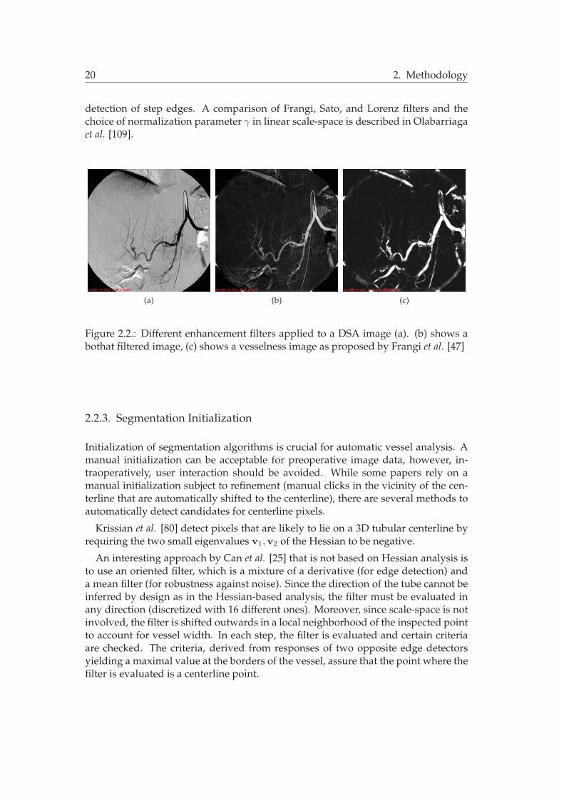
detection of step edges. A comparison of Frangi, Sato, and Lorenz filters and thechoice of normalization parameter γ in linear scale-space is described in Olabarriagaet al. [109].

(a) (b) (c)

Figure 2.2.: Different enhancement filters applied to a DSA image (a). (b) shows abothat filtered image, (c) shows a vesselness image as proposed by Frangi et al. [47]

2.2.3. Segmentation Initialization

Initialization of segmentation algorithms is crucial for automatic vessel analysis. Amanual initialization can be acceptable for preoperative image data, however, in-traoperatively, user interaction should be avoided. While some papers rely on amanual initialization subject to refinement (manual clicks in the vicinity of the cen-terline that are automatically shifted to the centerline), there are several methods toautomatically detect candidates for centerline pixels.

Krissian et al. [80] detect pixels that are likely to lie on a 3D tubular centerline byrequiring the two small eigenvalues v1,v2 of the Hessian to be negative.

An interesting approach by Can et al. [25] that is not based on Hessian analysis isto use an oriented filter, which is a mixture of a derivative (for edge detection) anda mean filter (for robustness against noise). Since the direction of the tube cannot beinferred by design as in the Hessian-based analysis, the filter must be evaluated inany direction (discretized with 16 different ones). Moreover, since scale-space is notinvolved, the filter is shifted outwards in a local neighborhood of the inspected pointto account for vessel width. In each step, the filter is evaluated and certain criteriaare checked. The criteria, derived from responses of two opposite edge detectorsyielding a maximal value at the borders of the vessel, assure that the point where thefilter is evaluated is a centerline point.

2.2. Vessels in Medical Images 21

2.2.4. Segmentation

If we pick up definition 1.3 from chapter 1, segmentation is the partitioning of theimage domain Ω into sets Sk ⊂ Ω, which satisfy

Ω =K

k=1

Sk (2.7)

where Sk ∩ Sj = φ for k = j and each Sk is connected [120].In our scenario, we only have two classes, S0, the background, and S1, the vascu-

lar object, i.e. segmentation yields binary images. Segmentation will also be calledlabeling, where a label (object or background label in our scenario) is assigned to a pixelif it is a part of the vascular object, or the background, respectively, see Figure 2.3.

(a) (b)

Figure 2.3.: (a) a volume rendering of a 3D CTA scan, (b) the segmented liver vascu-lature.

We identify two classes of segmentation algorithms that are interesting in our con-text, techniques based on Thresholding and Level Set methods.

Thresholding-Based Segmentation Methods Thresholding is a simple segmenta-tion algorithm that assigns object labels to pixels with an intensity that lies within aspecific range. The borders (thresholds) of this range can be determined manually orautomatically as proposed for vessel segmentation of MRA TOF images by Wilsonand Noble [155]. They model pixel intensities with different probability distributionsand iteratively solve for a classification using a Gaussian mixture model and the EM

algorithm [37].

22 2. Methodology

Condurache et al. [34] propose a hysteresis thresholding method, which computesa hard and a weak threshold and shifts pixels from the low confidence level (givenby the weak threshold) to the high confidence level (given by the hard threshold) viaadjacency.

Region Growing or Connected Thresholding only considers pixels in the intensityrange, which lie within the neighborhood of a seed point. It is suitable for segmen-tation of topologically connected objects, which generally can be assumed for vesselstructures. Selle et al. [134] propose a region growing technique for vascular images,where the intensity range to be considered is automatically determined by samplingthresholds and calculating the point in threshold space where the number of pixelswith object label significantly increases. At this point, it is assumed that the regiongrowing “breaks out” of the vascular structure and accumulates surrounding tissue.

Level Sets Segmentation based on active contours [72, 158] has become famous inComputer Vision and Medical Image Analysis. The intuition behind active contoursis to define a curve (the contour) and let it evolve in time depending on internal(smoothness) and external (image) forces. While early models use a parametric rep-resentation of the curve, Level Set methods [111, 26, 28] implicitly represent a curveas the zero Level Set of a higher dimensional function.

A Level Set method based on the evolution of a 1D curve in 3D for vessel segmen-tation has been proposed by Lorigo et al. [92], where the focus particularly lay onthe extraction of small vessels that cannot be found by mere thresholding. A gen-eral problem of Level Set methods evolving 2D surfaces for elongated structures istheir tendency to leakages where no high gradient is given. Deschamps et al. [38]introduce a freezing value for pixels indirectly proportional to their distance to thestarting seed point. If a point is very near the starting point but still on the evolvingsurface of the curve, it is assumed to be at a vessel border and it is set fixed. Nain etal. [104] incorporate a soft shape prior into the Level Set formulation that penalizesleakages. The prior is based on a filter yielding a large response if evaluated in asegmented region with a radius larger as the largest expected vessel radius.

Current research on vessel segmentation using Level Sets tries to localize smallvessels in MRA data sets continuing the work of Lorigo et al. [92]. Yan and Kassim[159] propose a Level Set formulation based on capillary forces in order to extractsmall vessels in MRA data. Their energy functional consists of several energy termsderived from the physics of capillarity. Gooya et al. [53] combine the Chan-Veseactive contour model [28] with the maximization of the product of two statisticaldistances and a flux maximization flow as proposed by Vasilevskiy and Siddiqi [149].

2.2.5. Quantification

Quantification of vessel structures is a main issue for feature-based registration ofangiographic images and a proper visualization. The main characteristics of vascu-lature that are subject to extraction are:

• Centerline: Since vessels have the structure of a tube, we are interested in its

2.2. Vessels in Medical Images 23

centerline, i.e. the 1D curve that describes the geometric shape of the vessels.

• Branching points: The topology of vessel structures is described by bifurcations.Vessels often have a tree-like shape, where junctions are distinct and can thusbe used for registration.

• Diameter: The width of the vessel tubes at all locations is an important criterionfor matching and visualization.

For some applications, such as classification of stenosis width, an estimate of the ves-sel wall is desired [46], which we will not cover since the registration task does notrequire models of the vessel wall. Given segmented vessel structures, methods havebeen developed to extract all the aforementioned information. However, there arealso direct methods, which quantify vessels based on grayscale information circum-venting the sometimes tedious and error-prone segmentation steps. The quantifica-tion of both segmented and grayscale images will be discussed in the following.

Centerlines from Segmented Images Given binary images, centerlines can be com-puted by producing a skeleton as introduced by Blum [14], who constituted the well-known medial axis transform (MAT). A skeleton represents the medial axis, which isthe set of centers and radii of the maximal disks that are contained within the object.There is a considerable body of research on skeletonization algorithms [13, 17]. Fastapproximative algorithms have been proposed for skeletonization, usually referredto as topological thinning algorithms [82]. Thinning algorithms remove points fromthe segmented object if their deletion does not lead to topology change or shrinkageof the segmented object.

An effective thinning algorithm particularly tailored for tubular structures is pro-posed by Palagyi [113] (see Figure 2.4c). This sequential algorithm iteratively testsborder5 points whether they are simple6 and non-final7, in which case they get re-moved. Special care is taken to symmetrically thin the structure by processing onlyone direction (north, south, east, west, and, for 3D, also bottom, and top) at a time.

A similar approach was proposed by Selle et al. [134] who guarantee the symmet-ric thinning by only removing simple points in the current pass if they have the samevalue in a Euclidean distance map [16] (see Figure 2.4a) computed on the segmenta-tion.

In general, skeletonization algorithms do not yield the centerline of tubular struc-tures, but introduce spurious branches, which have a smaller length than the diame-ter of the vessel in which they are located (see Figure 2.4c). In order to remove thesespurious branches, the analysis of a distance map can be used. For instance, brancheswith a length smaller than 2 times the diameter of the outgoing bifurcation can bedeleted. Or, as proposed in Selle et al. [134], pixels of the thinned structure whose

5A point with object label is called border if it is 6-adjacent (in 3D, 4-adjacent in 2D) to at least onebackground point

6A point is called simple if its removal does not change the shape’s topology. For a formal definitionrefer to [97]

7A point is called non-final if it has more than one object neighbor

24 2. Methodology

gradient magnitude in the distance map of the segmentation is not near to zero canbe discarded, assuming that only centerline pixels lie on a prominent intensity ridgeof the map.

Ridge Detection and Traversal Since we are often only interested in centerlinesand vessel diameters, approaches have been proposed to directly extract this infor-mation from greyscale images without segmenting the image.

Referring to the figure of a tube model (Figure 2.1), the intensity profile on a scan-plane orthogonal to the tube describes a 1D intensity (height) ridge in 2D [40]. In 3D,there is also a 1D ridge following the centerline of the tube, but cannot be visualizedas easily as the 2D pendant. Such ridges can be detected and traversed in the direc-tion of the tube. The detection of intensity ridges on images can also be interpretedas finding the medial axis on grayscale images, as proposed by Wang et al. [153] for2D images. Here, the MAT is based on maximal gradient responses from opposingboundaries (gradient medial axis transform, GRADMAT).

The group around S. Pizer laid the theoretic foundations of the detection of 1D in-tensity ridges8 by formally defining medialness for grayscale images, thus extendingthe definition of Blum [14]. Similar to Wang et al. [153], a measure for medialnesscan be derived by accumulating responses from opposing boundaries [121]. Themeasure is maximal at ridge points and thus suitable for detection.

Ridge traversal is achieved by moving along the ridge’s tangent direction, whichcan be approximated by the largest eigenvalue of the Hessian matrix [6].

The detection and traversal of ridges in vessel shapes yield the centerlines of thevessels, directly inferring a quantification of vessel structures, see Figure 2.4b. Ridgedetection is run in linear scale-space where the standard deviation of the Gaussianfilter σ is equal to the radius of the vessel whose centerline has been detected. Sinceridge detection and traversal yields two of three quantification results of vessel anal-ysis without explicitly segmenting the structure, it has received a lot of attention inthe Medical Image Analysis community.

For ridge detection, usually gradient and Hessian information of the image ismixed (gradient for extremum/boundary detection, Hessian eigenvectors for direc-tional information). Given a 3D image I, the gradient ∇I, the Hessian HI , theireigenvalues (v1,v2,v3) together with their corresponding ordered eigenvalues λ1 ≤λ2 ≤ λ3. As pointed out in the discussion in section 2.2.1, a ridge point has to fulfillcertain conditions in an intensity profile with bright vessel structures [40]

(i) Eigenvalues: The eigenvalues of the eigenvectors orthogonal to the tube mustbe negative.

λ1 ≤ 0 and λ2 ≤ 0 (2.8)

(ii) Optimum: The ridge point must be an intensity maximum in the directionsorthogonal to the tube. Thus, the projection of the gradient at a ridge point

8Together with the scales (radii) where they have been detected, 1D intensity ridges were also dubbedas cores [50]

2.2. Vessels in Medical Images 25

(a) (b) (c)

Figure 2.4.: (a) 2D Distance Map of a segmented DSA image (original: Figure 2.2a),(b) ridges responses as described in Koller et al. [79], (c) thinned image applied to asegmentation of (a) using the method of Palagyi et al. [113].

onto the directions (v1,v2)) must be zero at scale s for a tube with radius s:

v�1 ∇I = 0 and v�2 ∇I = 0 (2.9)

Using these criteria, ridge points and thus vessel centerlines can be detected [6]. In2D, only two instead of four criteria are tested.

Approaches by Koller et al. [79] and Krissian et al. [80] derive a filter response fromgradient and Hessian. Both methods use the fact that the gradient should be high atthe boundaries of the tubular structure, if it is measured orthogonal to the axis ofthe tube. At scale s, they measure the rate of intensity change along a directionorthogonal to the tube by

R(x) = min (∇I(x± sv1|2)�v1|2), (2.10)

in [79] and

R(x) =α=2π

α=0∇I(x± svα)�vα), (2.11)

where vα = cos αv1 + sin αv2 in [80].9

Again, the same criteria and response functions can be applied to 2D images, col-lapsing the circle described by vα to a line and probing two points (x ± sv1) on thisline.

The approach by Frangi et al. [46] finds ridges by fitting a 1D B-spline curve (whichis created manually) to the underlying data using an active contour model [72]. In-ternal forces account for smoothness of the curve while external forces attract thecurve toward a maximal vesselness filter response [47] and thus an intensity ridge.

The drawback of methods based on intensity ridges is that branching points can-not be detected easily since the filter responses are not high and ridge criteria do nothold at bifurcation points.

9In both Equations vi must be normalized.

26 2. Methodology

Detection of Branching Points Detecting the bifurcations of vessel structures is ofmajor interest for registration algorithms, since junctions represent distinct features,which can be used for matching. Given a segmented or thinned vasculature and aseed point, a wave can be defined propagating through all object pixels and testingfor connectivity of the front. This wave propagation algorithm has been proposed byZahlten et al. [162] for the use in hepatic vessel analysis. Size and direction of thewave have to be computed in each step if no centerline was extracted before.

Fridman et al. [50] detect branches with a cornerness measure derived from theimage gradient and the main direction of curvature (eigenvector v3 of the Hessian).The removal of false positives can be achieved by monitoring absence of a rapidchange of medialness responses in a local neighborhood of the current ridge point.

Krissian et al. [80] detect junctions in vessel structures by analyzing the distanceof adjacent vessel segments. If the distance between the endpoint of a vessel and theaxis of a second vessel is smaller than the radius of the second vessel, a junction hasbeen detected and the vessel segments are connected.

Diameter Computation Approaches that operate in linear scale-space have thenice side-effect that the standard deviation of the current Gaussian kernel, σ, atwhich a maximal response or ridge is detected, is equal to the radius of the vessel atthat ridge point [86].

If the centerline has been extracted from a segmented image, we can also measurethe diameter using a distance map [16] yielding the Euclidean distance to a contourof the segmentation (Figure 2.4a). If we assume, due to errors in the extraction pro-cess, that the centerline point is not located exactly in the middle of the segmentedtube, we can optimize the diameter computation by searching for the highest valueon the distance map perpendicular to the centerline direction.

2.2.6. Suggestions for Method Selection

The choice of the right vessel analysis method is very dependent on modality andpurpose. Current research is focused on detection of small vessels in 3D (mostlyMRA and CTA) images, where the purpose is mostly visualization and diagnosis.When it comes to intraoperative navigation (and feature-based registration), fastmethods have to be used that require little interaction and deliver results of rea-sonable quality also on 2D images, whose vessel extraction is, due to lower SNR anddimension and thus less information, not easier.

The purpose also chooses the method since a segmentation is only required in vi-sualization and measurements on vessel walls, while for registration tasks, a quan-titative analysis yielding topology (in terms of birfurcations), centerlines, and vesseldiameter, is often sufficient (which can be achieved without segmentation as in ridgetraversal techniques).

Thresholding or region growing methods are usually computationally efficientand yield decent segmentation results on 2D and 3D vascular images. However,region growing requires seed point initialization and both techniques suffer fromthe absence of a model, which often leads the algorithm to oversegmentation. A

2.3. Medical Image Registration 27

conservative choice of the threshold can avoid this effect, but the result will notgive the complete vascular tree making these methods not very suitable for a di-agnostic purpose. Combining thresholding techniques with the appropriate (model-based) filter enhancement and an automatic seed point detection can circumventthese drawbacks in order to have a good trade-off between computational efficiencyand accuracy.

A general problem in Level Set and Ridge Traversal methods is to deal with ram-ification locations. At these points, sharp corners10 are penalized by the Level Setapproach since the low curvature of an evolving curve or surface is not given. More-over, the inherent possibility of topology changes of Level Set methods, making themso powerful, is not desired in the context of vessel analysis assuming vessel struc-tures to be connected. Ramifications cannot be detected by ridge traversal methodssince the intensity ridge is not distinct at these locations. Thus, such methods tend torequire several starting seeds or reinitialization phases, which, to this end, cause fur-ther user interaction. The computational cost of Level Set methods and multi-scaleapproaches must not be underestimated since time is a critical issue especially intra-operatively. Both methods tend to require the fine-tuning of a number of parametersthat need to be adjusted for each modality. However, the ability to deal with smallervessel branches, which cannot be located by thresholding-based techniques, makeLevel Set and Ridge Traversal methods interesting due to their accuracy: the localinjection of contrast and magnification yields vessels in 2D whose corresponding3D vessels are very small. Their detection in 3D would improve 2D-3D registrationalgorithms in accuracy and robustness.

2.3. Medical Image Registration

After the introduction of vessel extraction and quantification techniques, which pro-vide the features for angiographic registration, the process of using these features foralignment, i.e. registering the underlying images will be focused.

Definition The process of image registration tries to find a transformation betweentwo or more images. In this thesis, we will constrain the registration task to two im-ages, the more general registration of multiple images, also referred to as mosaicking,will not be discussed.

Definition 2.1 (Registration of 2 Images) Given two images A : ΩA → R and B :ΩB → R and a set of admissible transformations ϕ : ΩA → ΩB, image registration isthe computation of a transformation ϕ′ that aligns A to B such that a certain comparisoncriterion, an energy E , is minimized:

ϕ′ = arg minϕE . (2.12)

10which usually occur at these junctions

28 2. Methodology

The choice of the energy depends on the set of admissible transformations. Theenergy E , also called error, or cost function, always contains a data termD, which mea-sures the quality of fit of the two data sets given a transformation. Moreover, as willbe discussed in section 2.3.2, E can impose constraints on the set of admissible trans-formations if it is not restricted by a model. The notion of correspondency is stronglyrelated to image registration. The input data must have corresponding informationin order to compute the transformation and evaluate a data term. Establishing thesecorrespondences depends on the technique chosen to register the images and willbe discussed in section 2.3.3. Since we try to find a minimum of a function (E), wealso need to incorporate some kind of optimization into our registration algorithm.Suitable techniques will be addressed in section 2.3.4. Section 2.4 will provide detailsof the necessary modifications and extensions that have to be applied when movingto multi-dimensional registration, in particular 2D-3D registration.

Literature A good introduction into basic concepts and algorithms of medical im-age registration is given in the book Medical Image Registration [61]. A thorough cat-egorization of registration techniques is presented by Maintz and Viergever [95] intheir Survey of Medical Image Registration. An interesting work is also the book Numer-ical Methods for Image Registration [103], showing registration concepts from a rathermathematical and general, but comprehensive and thorough point of view.

2.3.1. Data Terms

Image Registration can be approached in at least two different ways. Either imagefeatures are extracted and the registration is performed based on the extracted spa-tial information. This approach is referred to as feature-based registration. The secondtechnique directly performs the registration on the image intensities without requir-ing a previous feature extraction step. We usually speak of intensity-based registrationto address the latter approach. The difference between intensity- and feature-basedregistration is the choice of data term D.

Similarity Measures Intensity-based techniques use the intensity mapping of theimages to define a similarity measure (SM) as data term DS . If HA = {hA|hA : ΩA →R} and HB = {hB|hB : ΩB → R} are spaces of images A and B respectively, asimilarity measure can be described as

DS : HA ×HB → R (2.13)

For these similarity measures to be evaluated, the image must be transformed to-gether with its intensities, which brings up the issue of interpolation. Correspon-dency is assumed to exist at every pixel location in an overlapping region, and thesimilarity measure calculates the quality of fit given this correspondency inducedby transformation ϕ. Usually three categories are distinguished between similaritymeasures: difference-based measures calculating a function of the difference of inten-sity at each location, correlation-based measures computing the statistical correlation of

2.3. Medical Image Registration 29

intensities11, and entropy-based measures, determining the amount of signal entropybetween the two images12. For a good overview and mathematical definitions ofsimilarity measures, refer to [62].

Distance Measures Feature-based methods typically minimize a distance measureDD accumulated over all extracted features FAi ∈ ΠA, i = 1 . . . n, and FBj ∈ ΠB,j = 1 . . . m, where ΠA, ΠB are feature spaces of A,B, respectively. DD is usuallydefined via a metric d(., .) induced on the feature spaces, and an operator C assigningcorrespondences:

DD =n�

i=1

d(FAi , ϕ(C(FAi , {FBj })))2, (2.14)

where {FBj } ⊂ ΠB is a finite subset of features from image B, and C(FAi , {FBj }) = FBk ,if feature FAi corresponds to feature FBk . Correspondences can be established in aprevious step, or during the registration procedure (see section 2.3.3). Mind thatfeatures can be anything extractable from images, for which a distance function canbe defined and correspondence can be established. Common features in medicalimage registration include points, lines, (parameterized) curves, or (triangulated)surfaces.

Commonly used distance measures are Euclidean and the more general Mahalanobisdistance, both defined on points in Euclidean space R

n. Since most features can besampled by points, these are the most frequently used distance measures for MedicalImage Analysis and will thus be formally introduced.

Definition 2.2 (Euclidean distance) The Euclidean distance of two points X = (x1, . . . , xn)�

and Y = (y1, . . . , yn)� is defined as

d(X,Y)2 =�

(X−Y)�(X−Y) =�

(x1 − y1)2 + · · ·+ (xn − yn)2. (2.15)

Note that two points must have the same dimension for the Euclidean distance to beevaluated.

The Mahalanobis distance takes the statistical distribution of points into account.Intuitively, this distance emphasizes the statistical contribution of the different en-tries of two points in R

n to the distance measure. Weighting factors of the entries,expressed by their (co-) variances, are included in the distance measure.

Definition 2.3 (Mahalanobis distance) Given two points X = (x1, . . . , xn)� and Y =(y1, . . . , yn)�, interpreted as random vectors with covariance matrix Σ ∈ R

n×n, the Maha-lanobis distance is given by

d(X,Y)Σ =�

(X−Y)�Σ−1(X−Y) (2.16)

11making the measure independent of linear intensity changes12particularly suitable for inter-modality registration

30 2. Methodology

Of course, the choice of the distance measure should match with the chosen fea-tures to align. For instance, the distance of curves in R

n can be measured with theHausdorff or the Frechet distance [2]. However, since such distance measures aresometimes costly to compute (e.g. they require a parameterization) or are sensitiveto outliers, and since all geometric features can be sampled by a set of points, veryoften only the sum of the distances of each point in FA to the nearest point in FB iscalculated. If FA can be sampled by set {Xi}, i = 1, . . . , n, and FB can be sampledby set {Yj}, j = 1, . . . , m, a distance can be defined by

D({Xi}, {Yj}) =n�

i=1

minj

d(Xi,Yj), j = 1, . . . , m, (2.17)

where d(., .) is the Euclidean or Mahalanobis distance. Moreover, building a dis-tance map [16] of special distance metrics is not possible as they are not defined onall points on a grid resembling an image. Thus, improvements in performance viadistance look-up, which are important for many feature-based registration methods,are very difficult to achieve when not using point-based distance measures.

To summarize, intensity-based methods are approaches defined by means of sim-ilarity and interpolation, while feature-based methods are techniques defined bymeans of distance and correspondence.

2.3.2. Transformations

In general, we can distinguish between global transformations, where ϕ follows a pre-defined global model, and local transformations, where ϕ is less restricted by design,but the energy E constrains its behavior.

Global Transformations There are a number of transformation models used inMedical Image Analysis , which define a mere global transformation, discardingany deformation movement in data sets. We will briefly introduce the most impor-tant mono-dimensional mappings. The projection, a global transformation mappingfrom a higher to a lower dimension, will be subject to more attention in section 2.4 asit is the focus of this work. The other models are introduced since the 2D-3D modelcan be derived from them.

If a global transformation model is used, the set of admissible transformations isconstrained by design and the energy term E from Equation (2.12) only contains thedata term D, rendering the registration problem as:

ϕ′ = arg minϕD. (2.18)

A simple transformation model relies on the assumption of a global rigid move-ment. That is, all objects that ought to be registered do not change shape, only theirpose changes. Moreover, objects in the observed scene change their pose accordingly.Thus, the transformation can be casted as a global rotation and translation, which isapplied to all points X ∈ ΩA in the image domain:

2.3. Medical Image Registration 31

ϕ(X) = RX + t, (2.19)

where R is a rotation matrix and t a translation vector. In 3D, R ∈ SO(3) canbe defined via different parameterizations, e.g. Euler angles, unit quaternions, oraxis-angle representation. These parameterizations express the three degrees of free-dom (DOF) either by three parameters, or by four parameters and an additionalconstraint. Details of parameterizations are not immediate subject to discussion inthis section. However, since the choice of rotation parameterization is important forimplementation issues of the proposed methods, we refer the reader to appendix C,where our choice of parameterization, Euler Angles, is justified. A 3D rigid transfor-mation sums up to 6 DOF (3 for rotation, 3 for translation). Sometimes, an isotropicscaling factor is also added to the rigid model in order to account for different pixelsizes of A and B. We will discard this scaling since we assume A and B to be resam-pled adequately, or their extracted features to be given in mm.

There are other global transformation models, which soften the rigidity constraintsof Equation (2.19).

The affine transformation model allows for shearing and anisotropic scaling ad-ditional to the rigid transformation. It is often used as a local approximation of aprojective warp.

The projective transformation model13 is the most general global linear transforma-tion and is simply a linear mapping that must be invertible. This definition is alsocalled a homography as defined e.g. in [66].

As described by Rueckert [63], there are also non-linear global models, but theyare not frequently used in Medical Image Analysis and are thus not discussed.

Except for the rigid model, there is in general no reason why medical data shouldtransform according to a more general global model. Using these less restrictiveglobal models in image registration is either an approximation to the more gen-eral set of local transformations that describe e.g. tissue deformation, or applied tovery special problems like pixel size correction [67] or gantry angle estimation [138].However, since deformable registration (and thus local transformation models) hasreceived more attention and is better understood, current works tend to either usethe most restrictive rigid model to register objects that do not change shape (as, e.g.,bones) or to initialize a deformable refinement, or they use the most general localtransformations (introduced below) to register deformable objects.

Local Transformations In contrast to global transformation models, local transfor-mations do not restrict the movement of spatial locations in the first place.

By applying local transformations, which are also called displacement fields, spa-tial locations can be transformed (displaced) arbitrarily, which emphasizes the ill-posedness14 for the registration process using these types of transformations. In

13not to be mixed up with the projection transformation model14Informally defined, a registration problem is ill-posed if a) no solution exists, or b) it has no unique

solution, or c) if small changes in input lead to large changes in output. For a formal definition ofwell-posedness and its contrary refer to [60]

32 2. Methodology

order to counteract this inherent ill-posedness, restrictions are imposed on the trans-formations. These restrictions shall avoid “unnatural” transformations, i.e. a tearingor folding of spatial locations must not happen.

A mathematical way of defining transformations that fulfill these restrictions is thenotion of diffeomorphism, see for example [84, 18]:

Definition 2.4 (Diffeomorphism) Given two manifolds M and N , a bijective map f isa Cr diffeomorphism if both f : M → N and its inverse f−1 : M → N are r timescontinuously differentiable.

From this definition, we can deduce a local behavior of diffeomorphisms, which ismore intuitive for our means:

Theorem 2.5 (Local behavior of diffeomorphisms) If U and V are two open subsets ofR

n, a differentiable map f from U to V is a diffeomorphism at point x if

(1) f is bijective

(2) the derivative of f at x is invertible (has a non-zero determinant of the Jacobian)

Theorem 2.5 can be shown via the theorem of inverse functions, but is not within thescope of this thesis.

The bijection assures an invertibility of f , while the invertibility of the derivativeassures a smoothness of the mapping. Of course, a projection can never be a diffeo-morphism since its derivative cannot be invertible.

In practice, these diffeomorphisms are rather difficult to construct and impose ondifferent transformations. Thus, the diffeomorphic rule is sometimes loosened andtransformations are only required to be sufficiently smooth, i.e. the derivative of thetransformation is to be “well-behaved”, but ϕ and its derivatives are not necessarilyinvertible. This smoothness criterion is incorporated into the energy E additionallyto the data term and Equation (2.12) becomes

ϕ′ = arg minϕD + αS, (2.20)

where D is the data term depending on the input data, and S is a smoothing termimposing constraints on the set of admissible transformations ϕ. The scalar α is aregularization parameter controlling the influence of the smoothing criterion.

Typically, the smoothing term S is a function of the derivatives of ϕ. A popularchoice of S is the diffusion regularization term [154, 103] penalizing for the sum of thefirst derivatives of ϕ:

SD =n�

i=1

�Ω

���∇ϕ(i)���2

, (2.21)

where ∇ϕ(i) ∈ Rn is the gradient w.r.t. X of the transformation in dimension i. 15

15Mind that ϕ is a vector-valued function, and its first derivative is a Jacobian matrix J ∈ Rn×n.

2.3. Medical Image Registration 33

Since the diffusion regularization term is sensitive to affine transformations, whichis not desired in some scenarios (where the unknown transformation also includes arigid part, for example a rotation), a regularization term that penalizes the curvatureof the displacement field has been proposed

SC =n�

k=1

�Ω

n�i=1

n�j=1

�����∂2ϕ(k)

∂xi∂xj

�����2

, (2.22)

where ∂2ϕ(i)

∂xi∂xjis the the second derivative with respect to xi and xj . This regulariza-

tion term is often called bending energy [128] or Thin-Plate energy functional (see Ap-pendix B, Equations (B.3) and (B.4)) and inherently permits affine transformations,since SC(Ax + t) = 0. This term must not be mixed up with a so-called curvature reg-

ularization term,�n

i=1

�Ω

���Δϕ(i)���2, as proposed by Fischer an Modersitzki [42], which

leaves out the mixed terms of the second derivatives and is an approximation toSC

16.Other regularization terms have been proposed in the literature, partly based on

physical properties, but are not subject to discussion here. For a summary of fre-quently used regularization terms, refer to [103].

In Medical Image Analysis , diffeomorphisms and their (regularizing) approxima-tions are called deformations, thus the term deformable registration.

Parametric vs Non-parametric Transformations We can distinguish between trans-formations expressed with or without parameters, raising the terms parametric andnon-parametric registration.

Parametric transformations use models of a transformation which are expressedwith a set of (few) parameters. If these parameters are known, they can be put intothe transformation model and all spatial locations can be transformed. Global trans-formations are always based on models and thus belong to this class of transforma-tions.

Particularly suitable for feature-based deformable registration are Thin Plate Splines(TPS), and their diffeomorphic extension, Geodesic Interpolating Splines [24], since theycan register features with arbitrary locations, are minimizing the Euclidean (or Ma-halanobis) distance between features, and keep the transformation smooth by min-imizing the Thin Plate energy functional. See Appendix B for mathematical deriva-tion, numerical computation, and application of TPS to Medical Image Analysis .

There are also other models that are often used for deformable registration. FreeForm Deformations (FFD) are used to interpolate transformations defined on a reg-ular grid. B-spline interpolants [128], also shown to yield diffeomorphisms [30, 127],are typically used for intensity-based registration, since they offer a smooth interpo-lation with local support17. Due to their local support, FFDs only yield meaningfuldeformations if a set of features is well distributed over the whole image domain.Thus FFDs are not very suitable for feature-based registration.16Δ is the Laplace operator, i.e. the sum of second derivatives without the mixed terms17meaning that a grid node only influences the transformation in a local neighborhood

34 2. Methodology

Non-parametric transformations do not consider a model of the transformation,but only address the transformation ϕ as a function. Solving for this function is thetask of image registration. Since the energy of Equation (2.12) depends on ϕ, E be-comes a functional, which is to be minimized. The minimization of functionals, whichincludes the calculus of variations, is not in the scope of this thesis, but the readeris referred to Modersitzki [103] for introduction and to Zikic [164] for a numericalsolution of this problem.

2.3.3. Correspondences

With transformation ϕ′ from Equation (2.12) we want to reestablish the correspon-dency between imagesA andB. Correspondency can be specified in terms of anatom-ical corresponding features, image-based feature correspondences, or pixel corre-spondences.

As already mentioned, in intensity-based approaches, correspondency is assumedto be given at every pixel location in a region where the two images overlap, i.e.ΩA,B = {x ∈ ΩB|ϕ−1(x) ∈ ΩA} [61], and fully depends on the given transforma-tion. That means a pixel location of the first image corresponds to the nearest pixellocation of the transformed second image.

In feature-based approaches, the correspondence problem is more important andis thus subject to discussion in the following. Here, correspondency can be18 re-garded as being dual to transformation: Given two sets of features FA ∈ ΠA ex-tracted from A and FB ∈ ΠB extracted from B. If correspondency is given for FA,FB, usually we can determine the transformation ϕ. Vice versa, if ϕ is given, we canestablish correspondences for the whole image domains ΩA, ΩB, and hence for FA,FB. A good review of existing algorithms for finding feature correspondences canbe found in Chui et al. [31].

Mathematically, the problem to solve is to find a bijective or one-to-one mappingbetween the feature sets FA, FB. This problem was casted as a graph matching orquadratic assignment problem by Shapiro and Haralick [135], see also Gold and Ran-garajan [51].

Given two graphs G = (VG, EG) and g = (Vg, Eg), where VG = FA and Vg = FB,and EG, Eg express a relationship of features, which lie in the same feature set19.We want to find a bijective mapping f : VG → Vg, such that the relationships ofcorresponding features are most similar, i.e. we want to find M,M′ that minimize

−�

a

�

b

�

i

�

j

MaiM′bjCaibj , (2.23)

where M and M′ are permutation matrices, i.e. Mai = 1 if feature FAa correspondsto FBi and M ′

bj = 1 if FAb corresponds to FBj , respectively, otherwise they are 0.Caibj = 0 if (a, b) /∈ EG or (i, j) /∈ Eg, otherwise they express a cost of how good therelationships of the two feature tuples fit.18loosely19Such a relationship can for instance express the geometric or topological configuration of a feature

set.

2.3. Medical Image Registration 35

The problem of quadratic assignment is NP-hard, which is basically due to thecomparison of relationships. The Computer Vision community has come up withdifferent methods to circumvent the graph matching. We can distinguish betweentwo different classes of approaches.

Feature Descriptors Instead of comparing relationships, one can compare a scalarcost Cij yielding the quality of correspondence between two features FAi ,FBj . This re-duces the graph matching problem to a weighted bipartite graph matching or linearassignment problem (LAP). Now, we want to minimize the cost

−�

i

�

j

MijCij , (2.24)

which can be solved in polynomial time [115]. The cost matrix C can be establishedusing feature descriptors, which, in order to be suitable for feature-based registra-tion, usually have to be translation-, rotation-, scale-, and in the case of 2D-3D regis-tration projection-invariant. Feature descriptors have become rather popular in theComputer Vision community [93, 85, 8], however, they are not frequently used inMedical Image Analysis . This is most probably due to higher variations of inputdata, and the rather restricted applicability of feature descriptors fulfilling all theaforementioned invariants.

Alternating Approaches By using the “duality” between transformation and cor-respondency, different methods have been proposed to alternate between correspon-dence detection and transformation estimation. Most of these approaches use a clos-est point distance measure (Equation (2.17)) to update the correspondency, and thenreestimate the transformation. These closest point distance measures are not optimalin the sense of linear assignment, but they are generally faster, easier to implement,and yield a good approximation to the solution of Equation (2.24). Two algorithmsthat are frequently used in the Medical Image Analysis community are the IterativeClosest Point (ICP) algorithm proposed by Besl and McKay [11] and Zhang [163], andthe Robust Point Matching (RPM) algorithm proposed by Chui and Rangarajan [31].Due to its applicability to 2D-3D registration and its nice theoretical properties, wewill have a closer look at the former method.

The Iterative Closest Point Algorithm The task is to rigidly register two sets of 3D20

features (surfaces, curves, point clouds) sampled by point sets Xi ∈ FA, i = 1, . . . , nand Yj ∈ FB, j = 1, . . . , m. To this end, we want to find rotation R and translation tto minimize the energy

E =12

n�

i=1

m�

j=1

Aijd(Xi,RYj + t)2, (2.25)

where A is a permutation matrix.20Naturally, 2D features can also be aligned with the ICP

36 2. Methodology

The algorithm first updates A using a closest point operator (for instance Equation(2.17)) and then estimates the transformation given these correspondences (for ex-ample with a closed-form solution of the absolute orientation problem [147]). Thesetwo steps are repeated until the update of the transformation is smaller than a pre-defined threshold.

It can be shown [11] that this algorithm always converges. Moreover, as shownby Granger and Pennec [55], if the distance measure d(., .) of Equation (2.25) is theMahalanobis distance, and if the measurement error is assumed to be Gaussian, theICP is a Maximum Likelihood estimator. In its pure form, the ICP requires a rathergood initial estimate to converge to the right solution if outliers21 are present. At-tempts have been made to increase the robustness of the ICP by discarding pointsthrough statistical analysis [163], perturbing the locations of points in one featureset by random noise [116], or estimating the probability of the correspondences andcasting the ICP as an EM algorithm [55].

Mind that the ICP must not be mixed up with naive approaches where a cost func-tion with unknown correspondences is optimized (compare for example [1, 88]). Inthe latter case, in one iteration of the optimization, the correspondency is newly de-termined, and a cost function (energy) is evaluated once with these correspondences.The ICP, however, determines the correspondency and then optimizes the error (en-ergy term) based on these correspondences in a single iteration. Only after the algo-rithm has found a minimum, the correspondency is reestimated. The minimizationof the error in each iteration assures the convergence of the ICP, whereas convergenceof naive approaches is not guaranteed.

2.3.4. Optimization

Since Equation (2.12) requires a minimization of a function E , numerical optimiza-tion is an important issue for medical image registration. Some registration algo-rithms offer a closed-form solution by design22, or a simple iterative scheme whereconvergence is guaranteed.

Most of the algorithms, however, make use of optimization algorithms. Thesealgorithms solve the registration problem iteratively by refinement of parameterssuch that the energy term E decreases and becomes minimal. Depending on theenergy term, parameter-based optimization is achieved using direct methods andgradient-based methods. Besides these methods, especially non-parametric registra-tion problems can also be solved by building up a time-dependent or fixed-pointiterative scheme directly on the energy formulation (2.12), which is repeated to ob-tain a steady-state solution [103].

Direct Methods Direct optimization methods try to find a global minimum bysampling the parameter space. Especially for energy terms that change their number

21features that have no corresponding one in the other data set22for example a TPS registration (see appendix B)

2.3. Medical Image Registration 37

of input measurements, these methods are used instead of gradient-based optimiz-ers. The sampling can be done in different ways.

The by far easiest method is a Best Neighbor approach, where the energy is evalu-ated at all neighbors of a point in parameter space. The neighbor yielding the lowestenergy value is the next sampling point. These steps are repeated until no furtherimprovement of E can be found at the neighbors of the sampling point, which is as-sumed to be the global minimum in parameter space. Of course, this method needsa good initialization value since it is prone to fall into local minima.

A better way of sampling the parameter space to find a global optimum is theDownhill Simplex Method [107]. In an n-dimensional parameter space, a simplex (aset of n + 1 points in this space) is created and certain operations can be applied toit in order to find a global optimum. Depending on the values at all n + 1 points,the simplex can be reflected, expanded, or contracted in order to shrink, enlarge,or move the search region. If the simplex is shrunk smaller than a threshold, thealgorithm assumes to have found an optimum and returns the point of the simplexyielding the smallest energy value.

There are other direct methods, like simulated annealing, genetic optimization,Powell’s Method, etc. For a good reference refer to Numerical Recipes in C [123].For registration tasks, the Downhill Simplex method performs a rather good job ifgradient usage is not intended.

Gradient-Based Methods Gradient-based optimization algorithms look for the op-timum by analyzing the gradient, of the energy term E , sometimes in combinationwith its second derivative. At the optimum, the gradient should be zero. Startingfrom an initial estimate p0, a parameter update is computed in each iteration untilthe gradient vanishes (and the algorithm converges)23.

For a function F : Rm → R to be optimized and a starting point p0 ∈ R

m, we cangive a generic gradient-based algorithm:

Algorithm 1 Gradient-Based OptimizationGiven a function F and a starting point p0

p← p0

repeatcalculate parameter update Δp from F and its derivativesupdate parameters: p← p + αΔp

until ‖Δp‖ < ε

The important step is the calculation of the parameter update Δp. The parameterα determines how far to move in the direction determined by Δp. If not too time-consuming, α is determined via a line search along Δp.

A method that assures linear convergence (i.e. in each step the error reduces lin-early) is the gradient descent method. Here, the update is determined by the negative

23This test is usually performed via the magnitude of the update

38 2. Methodology

gradient direction (direction of steepest descent):

Δp = −F ′. (2.26)

A method that assures quadratic convergence (but is computationally expensive)is the Newton method. Here, F ′ is approximated with its Taylor expansion

F ′(p + Δp) = F ′(p) + F ′′(p)Δp +O(||Δp||2) (2.27)≈ F ′(p) + F ′′(p)Δp. (2.28)

From this, and from the assumption that F ′(pmin) = 0 at the minimum pmin of F ,we get the update Equation by solving for Δp

F ′′(p)Δp = −F ′(p). (2.29)

Note that the second derivative can be near to singular at some points in parameterspace, which makes the Newton algorithm less robust.

Very often, energy terms are defined by a squared norm of a vector-valued func-tion f , i.e.

F =12‖f(p)‖2, where f = (f1, . . . , fm)�. (2.30)

Here, we can also apply the gradient-decent and Newton method by computinggradient and Hessian:

F ′(p) = J(p)�f(p), and F ′′(p) = J(p)�J(p) +m�

i=1

fi(p)f ′′i (p), (2.31)

where J is the Jacobian of function f .From Equation (2.31) we can deduce an update step approximating Newton’s step,

which does not require the costly computation of the second derivative. Solve for Δpin Equation

J�JΔp = −J�f . (2.32)

This method is called the Gauss-Newton method, which sometimes gives quadraticconvergence as the Newton method.

There are also other algorithms for gradient-based optimization, for a nice overviewand description see Methods for Non-Linear Least Squares Problems [94].

2.4. 2D-3D Registration

Now that basic methodology of medical image registration has been introduced, wecan proceed to the description of 2D-3D registration concepts. After introducingthe general pinhole camera derived from Computer Vision, we will focus on theparticular scenario of intraoperative C-arms and explain calibration (section 2.4.2)and error analysis (section 2.4.3) in this context.

We refine the definition of section 2.3, registration of 2 images, to the particularcase of 2D-3D registration:

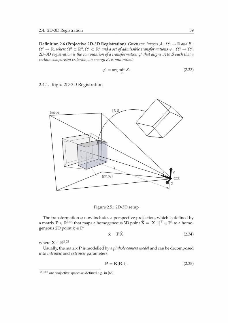
2.4. 2D-3D Registration 39

Definition 2.6 (Projective 2D-3D Registration) Given two images A : Ω3 → R and B :Ω2 → R, where Ω3 ⊂ R

3, Ω2 ⊂ R2 and a set of admissible transformations ϕ : Ω3 → Ω2,

2D-3D registration is the computation of a transformation ϕ′ that aligns A to B such that acertain comparison criterion, an energy E , is minimized:

ϕ′ = arg minϕE . (2.33)

2.4.1. Rigid 2D-3D Registration

Figure 2.5.: 2D-3D setup

The transformation ϕ now includes a perspective projection, which is defined bya matrix P ∈ R

3×4 that maps a homogeneous 3D point X = [X, 1]� ∈ P3 to a homo-

geneous 2D point x ∈ P2

x = PX, (2.34)

where X ∈ R3.24

Usually, the matrix P is modelled by a pinhole camera model and can be decomposedinto intrinsic and extrinsic parameters:

P = K[R|t]. (2.35)

24P

2|3 are projective spaces as defined e.g. in [66]

40 2. Methodology

For an illustration of the meaning of the parameters, refer to Figure 2.5. The cali-bration matrix K encapsulates the intrinsic parameters and is generally defined by

K =

���

fx s px

0 fy py

0 0 1

��� . (2.36)

Here, fx and fy account for the focal length in metric coordinates, i.e. fx = fmx,fy = fmy, where f is the focal length in pixel coordinates and mx, my are the dimen-sions of a pixel in metric coordinates in x- and y-direction, respectively. The entry sdenotes a skew factor accounting for non-rectangular pixels and is set to zero in mostof the cases. The point (px, py)� is the so-called principal point and denotes the inter-section of the positive z-axis of the camera coordinate system (CCS, whose origin islocated at the center of projection) with the image plane.

The matrix [R|t] encapsulates the extrinsic parameters, which is a rigid trans-formation (see section 2.3.2) moving all 3D points from the world coordinate system(WCS)25 to the CCS.

Estimating P is referred to as rigid 2D-3D registration. Note that this estimation isa non-linear task, since a perspective division must be carried out when going fromhomogeneous to inhomogeneous points, which are the actual image coordinates. Infact, if the rows of P are denoted by

P =

���

p�1p�2p�3

��� (2.37)

the actual projective mapping function fP : R3 → R

2 is given by

x = fP(X) =�

p�1 Xp�3 X

,p�2 Xp�3 X

��. (2.38)

2.4.2. Calibration

In normal camera systems the intrinsic parameters do not change and have to be de-termined one time only in a calibration step. For C-arms, phantoms with implantedfiducials are typically imaged to recover the projection matrices and thus the intrin-sic parameters in an off-line calibration step [89]. C-arms typically provide 2-3 zoomfactors with different focal lengths, all of which must be calibrated seperately. Thecalibration reduces the rigid 2D-3D registration to the estimation of the extrinsic pa-rameters, which is also referred to as 2D-3D Pose Estimation.

However, care has to be taken in 2D-3D registration of X-ray images coming from aC-arm. Due to the C-arm’s heavy weight, mechanical bendings of the C-structure ac-count for changes in the intrinsic parameters as the C-arm angulation changes. Thiseffect is increased if mobile C-arms are used. For a stationary C-arm Gorges et al. [54]

25also called the object coordinate system

2.4. 2D-3D Registration 41

reported an error of the y-entry of the principal point, py, while px and f remainedstable during angulation changes. Thus, the intrinsic parameter py depends on thechosen angle from which the X-ray is acquired, which has to be taken into account forrigid 2D-3D registration. As already mentioned in 1.2.2, state-of-the-art C-arms pro-vide a 3D reconstruction technique to produce 3D DSAs, or CT-like slices. For that, acalibration is carried out for all angulations of the C-arm from which projections aretaken for reconstruction. These positions are thoroughly calibrated [105].

The physical setup of C-arm devices introduces a distortion of the images due todetector geometry and earth magnetic field as described in 1.2.2. For 2D-3D regis-tration, this distortion has to be corrected, which can be achieved by fitting a high-degree polynomial to phantom data [161]. However, newer C-arms based on flat-panel technology do not produce distorted images, discarding the necessity of dis-tortion correction.

In summary, due to flat-panel technology and the information gained by a multiple-view calibration step for 3D reconstruction, intrinsic parameters can be assumed tobe given for almost every angulation.

In the following, the term “rigid 2D-3D registration” will be interpreted as therecovery of viewpoint or pose parameters, essentially the rigid transformation [R|t]aligning WCS to CCS. Thus, the number of parameters to solve for is 6 in the rigidcase, i.e. 3 for rotation and 3 for translation. Mind that the rigid 2D-3D registrationin the case of calibrated images tries to find a 3D transformation ϕ : Ω3

A → Ω3A′ . The

actual projective mapping is part of the energy E and is usually incorporated into thedata term.

2.4.3. Error Analysis

Several issues have to be addressed for evaluating the quality of a registration algo-rithm, and for performing thorough tests to analyze the error. Usually, one has tofirst cope with the creation of a reference solution to which the solution provided bythe proposed algorithm can be compared. Then, a reasonable error measure has to beapplied to assess the quality of fit (accuracy) of the registration compared to the refer-ence. This error measure should be as independent as possible from the energy usedfor optimization. Last but not least, the robustness of the algorithm has to be shown,i.e. how it behaves in special situations, how often it converges to the right solutionwhen applied with different input, and how much disturbance can be introduceduntil the registration fails.

Creating Ground Truth and Gold Standard For error assessment, it is importantto have a reference registration, i.e. registration parameters that are assumed to be“correct”.

For this, one can create a simulation: A previously known transformation is ap-plied to a 3D image, which is then projected to artificially produce a 2D image. Then,this transformation has to be recovered from the registration algorithm using 3D im-age and produced 2D image. In this case, our reference registration is called a ground

42 2. Methodology

truth registration, since we know the exact transformation. The problem in groundtruth creation is to create an artificial projection which simulates a real 2D projectionas much as possible (modeling noise, projected anatomy, etc.).

Another possibility to create a reference registration is to use a gold standard al-gorithm for the problem. For 2D-3D registration, usually reference registrations arecreated by implanting fiducials into the image and running a gold standard point-based registration with known correspondences. Another (less invasive) possibilityis to (manually) determine corresponding landmarks (e.g. bifurcations in vessel treesin the case of angiographic registration) and again performing a point-based regis-tration.

One of the currently favored approaches for a gold standard is to use a 3D recon-struction from the C-arm and perform a 3D-3D registration to the input 3D imageto yield transformation T3D−3D. Due to the optimized calibration of C-arms, theprojection matrices are known for all images from which the 3D reconstruction wascreated. Given one of these 2D views, its projection matrix P = K[R|t], and thetransformation T3D−3D, a “gold standard transformation” is given by

Tgold =�

R t0 1

�T3D−3D. (2.39)

This evaluation method only works if a 3D-3D registration algorithm is available,which allows for a calculation of a transformation. Usually, however, alignment of 23D images is regarded to be an easier problem than 2D-3D registration and thus, thecreation of such a reference registration is accepted even in deformable regions.

The reference registration can also be produced by an expert by manually alteringthe transformation parameters. This is only possible in the case of rigid registra-tion, since local changes can hardly be assessed even by clinical experts. Moreover,providing a suitable user interface to model more than 6 DOF is not a trivial task.

Accuracy Measurements Certain issues have to be addressed to define an error forsingle-view 2D-3D registration.

First, it is important to know that in all C-arm systems, the imaged object liesbetween the X-ray source and the detector system, making an error assessed in 3Dsmaller than the error assessed in the image plane26.

Second, the transformation perpendicular to the image plane is more difficult tosolve for and has to be assessed separately.

Van de Kraats et al. [148] have proposed a standardized protocol to assess theerror in 2D-3D registration (for an illustration see Figure 2.6). They propose to usepreviously defined 3D image points {Xi}, i = 1, . . . , n (e.g. sampled throughout thevolume of interest) to assess the mean target registration error (mTRE)

mTRE =1n

n�i=1

d(TregXi,TgoldXi), (2.40)

26Mind that it is only reasonable to give the error in mm, not in pixel, which is generally no problemfor all C-arm systems since they provide the size of a pixel in mm

2.4. 2D-3D Registration 43

Figure 2.6.: Different Accuracy Measures. Reproduced from van de Kraats et al. [148]

where d(., .) is the Euclidean distance of the inhomogeneous representation of points,and Treg is a registration computed with the algorithm to be tested.

Moreover, to assess an error without the bias in projection direction, v.d. Kraats etal. propose to use a mean reprojection distance (mRPD),

mRPD =1n

n�

i=1

dL(Li, TgoldXi), (2.41)

where Li is the ray connecting PregXi and the center of projection, and dL(., .) is thedistance of a point to a line in 3D. Evaluating the pixel error of the points Xi is alsosuggested, called the mean projection distance

mPD =1n

n�

i=1

d(PregXi,PgoldXi). (2.42)

Additionally to the protocol by van de Kraats et al. , the root mean square error(RMSE) in all the parameters is often evaluated, i.e. for a parameter Θ, which hasbeen estimated m times, the mean distance to the parameter value of the gold stan-dard registration Θgold is evaluated

RMSE =

�1m

m�j=1

(Θj −Θgold)2 (2.43)

44 2. Methodology

Moreover, mean and standard deviation of all parameter differences are importantvalues, especially the standard deviation, telling about the quality of the mean andthus the RMSE. Van de Kraats et al. reason that this error evaluation can be mislead-ing since the translation values are dependent on the center of rotation. However,if the center of rotation coincides with the origin of the WCS, these values are not“rotation-biased” and give a good hint of the accuracy of all parameters, which, in aglobal transformation model, are important to interpret. For local transformations,there are usually too many parameters to reasonably interpret the RMSE and stan-dard deviation. Thus, RMSE and standard deviation should only be assessed in rigid2D-3D registration, which sometimes gives a better insight into the algorithm’s be-havior than analysis of mTRE, mPD, or mRPD.

Robustness Assessment Robustness assessment tries to evaluate an algorithm withrespect to reproducibility in different scenarios with controlled disturbances. Cen-tral to all robustness measurements is to create a set of different scenarios and testwhether the algorithm can reach the right solution.

Usually, a representable amount of different instances of transformations is cre-ated and the algorithm is invoked. These are called Monte Carlo simulations. Thetransformations can be categorized into different ranges and the registration can beevaluated by the range until which it is still successful (the so-called capture range).In this context, a “successful” registration must be defined, which is a fixed thresh-old of the accuracy error function, usually inspired by clinical partners27. The rangeshould be defined in terms of the error with which the accuracy is measured. For in-stance, if the error is assessed using the mTRE, instances of the transformation mustbe created such that the mTRE lies within a certain range. An easier method is whenthe RMSE in the registration parameters is assessed, where only displacements in acertain range have to be added to all parameters.

Of course, creating different scenarios also involves testing the algorithm on dif-ferent data sets. However, the amount of different patient data to be tested to yielda reliable claim on the inter-patient reproducibility is usually never achieved in theliterature.

27Depending on the clinical application, an algorithm has to be accurate in terms of submillimeters orseveral millimeters

3. State of the Art in 2D-3D AngiographicRegistration

In the previous chapter, vessel extraction and registration methodology was intro-duced. Now, we will have a look at the state of the art of registration of angiographic3D images to 2D projections.

A review of algorithms for rigid 2D-3D registration of angiographic images will begiven in sections 3.1, 3.2, and 3.3 as they have been proposed in the literature.

The necessary methods like volumetric intensity projection and distance functioninterpretation will be provided in the respective sections.

This chapter concludes with a short summary of the few 2D-3D non-rigid regis-tration algorithms and a discussion, where future directions of research in this fieldwill be highlighted.

3.1. Intensity-based 2D-3D Registration

As already mentioned in 2.3.1, intensity-based registration evaluates a similaritymeasure directly on the intensity mapping of the images. In 2D-3D registration,however, the dimensions of the two images differ, so either the 2D projection mustbe backprojected into space to compare it with the 3D image intensities, or the vol-ume has to be projected to compare it with the 2D image intensities.

The former approach is usually used if more than one view is provided, and re-construction of intensities is feasible, compare, e.g. Tomazevic et al. [142]. Since weare more interested in 2D-3D registration based on a single view and since there isno work addressing multi-view 2D-3D registration on angiographic images via recon-struction, we will ban approaches based on backprojection from the discussion.

The latter approach, projecting the volume and evaluating a similarity measurein 2D, will be discussed in the following. The projection of the volume’s intensitieshas to be carried out such that the physical process of X-ray imaging is simulated.This simulated or reconstructed 2D image from 3D intensities is called a DigitallyReconstructed Radiograph, DRR. DRR generation can be particularly achieved whenusing CT images to align them with 2D X-ray images since their acquisition followsthe same laws of attenuation of radio densities. However, as we will see below, alsoMR data can be used to produce DRRs for angiographic registration if adequatelysegmented.

The process of 2D-3D intensity-based registration can then be summarized as anoptimization (see 2.3.4) of parameters Θ over an energy term. The energy evaluationreads as defined in algorithm 2.

46 3. State of the Art in 2D-3D Angiographic Registration

Algorithm 2 Energy Evaluation of Image-Based 2D-3D RegistrationGiven a 3D image A and a 2D image B, and parameters Θ

create a DRR from A using the projection matrix PΘ to produce ADRR

evaluate a similarity measure SM(ADRR,B)

Below, we will have a closer look at DRR generation for angiographic images, andin section 3.1.2 we detail algorithms for 2D-3D rigid intensity-based registration asthey have been proposed in the literature.

3.1.1. DRR Generation

X-ray Imaging The ionizing property of X-ray beams is used by CT(A) and intra-operative devices such as C-arms to acquire images. Images can be produced byradiation since different materials interact with the emitted energy of an X-ray beam1

in a different way, according to the material’s radio density. If a material interactswith the energy, part of the energy is lost during traversal. This “loss of energy” iscalled attenuation and can be physically described by the Lambert-Beer law for atten-uation of radiation through a medium: Given an initial energy E0 of an X-ray source,the remaining energy E of a ray traversing an object is given by

E = E0e−�

μ(x)dx, (3.1)

where μ(x) is the attenuation coefficient of the object at point x.

CT Hounsfield units CT intensities are measured in Hounsfield units, i.e. intensityvalues normalized by the attenuation of water:

H =μ− μW

μW1000, (3.2)

where μ is the attenuation coefficient of a certain material, and μW that of water.Putting this equation into Equation (3.1), we get [117]

EDRR = E0e−� �H(x)μW

1000+μW

�dx

. (3.3)

This formulation can be used to create DRRs from CT images.

Image Formation Using Equation (3.3)2 and a projection matrix P, an image can becreated by casting rays from the center of projection through every pixel of the imageplane and following the ray through the volume (see Figure 3.1). If a voxel is hit

1The energy of an X-ray beam must not be mixed up with the energy used for minimization. This willbe indicated by using different notations.

2To reduce the computational cost, usually its logarithm is used

3.1. Intensity-based 2D-3D Registration 47

during traversal, its Hounsfield value is contributing to the integral3. Since usual X-ray images are of size 512×512 or 1024×1024 pixels, this image formation process iscomputationally expensive. However, speed-ups can be achieved by approximatingray casting through blending of a 3D texture mapped volume, or by shifting raycasting to the Graphics Processing Unit (GPU) [75]. Other techniques adapted fromthe Computer Graphics community have been proposed for fast DRR generation[129, 12].

(a) (b)

Figure 3.1.: (a) A DRR generated from a CTA volume, (b) a real fluoroscopic image(inverted).

Radiometric Calibration For DRR generation, the energy EDRR has to be furtherprocessed to simulate the traversal of electrons through the intensifier, or the flatpanel detector imaging process. Only after this processing, the intensity IDRR canbe assigned to pixels. Different models have been suggested for simulation, but nonecan be favored since they are not modeling the physical process of image formation.Moreover, CT machines have a different effective energy with which images are ac-quired compared to intraoperative devices. Thus, different transfer functions4 are ap-plied to the volume intensities in order to simulate different effective energy levelsof CT image acquisition and intensifier/flat panel physics. An estimation procedureof the transfer function’s parameters, a radiometric calibration, can be carried out tomake the DRR most similar to a real radiograph as proposed by Khamene et al. [75].

DRR Generation for Angiographic Data For contrasted vessels, a logarithmic re-lationship can also be established between the remaining energy EDRR and the re-sulting intensity, i.e. IDRR = log[EDRR] [117, 81]. Thus, the intensity IDRR can be

3which is approximated by a sum in the discrete setting4A transfer function is a mapping of intensity values to a color map

48 3. State of the Art in 2D-3D Angiographic Registration

assumed to be proportional to the length L of the path traversed through the 3Dvessel and the contrast material’s density ξ [68]

IDRR ∝ μ�

Lξ(x)dx, (3.4)

where μ is the attenuation coefficient of the contrast material.Mind that this equation only holds inside a contrasted vessel, surrounding tissue

cannot be modeled thus. That is, in order to produce DRRs for angiographic data, avascular segmentation is usually necessary as a pre-processing step. However, sincethe density of contrast material can also be measured in MRA voxel intensities, andsince μ can be estimated by radiometric calibration, MRA images can be used forDRR generation as well as CTA images.5 Most methods for intensity-based 2D-3Dregistration of MRA data approximate this DRR generation with a Maximum Inten-sity Projection (MIP), where only the voxel on the ray with the highest intensity con-tributes to the pixel intensity. On the one hand, this method is prone to error causedby noise compared to a full integration over all vessel voxels on the ray. On the otherhand, however, no segmentation of the 3D vasculature is needed to produce DRRs.

3.1.2. Registration Algorithms

In the following, intensity-based 2D-3D rigid registration algorithms will be reviewed.All methods will be described by the input data their algorithms work on, the DRRgenerator which is used, the similarity measure defining the energy term, and theoptimization technique to reach a global optimum. Execution times and accuracyare hard to compare due to different hardware, non-standardized evaluation pro-tocols, and different input data. However, they are reported to give an impressionon runtime and performance, the reader is referred to the original publications for athorough explanation on experiments.

An extensive study of different similarity measures for 2D-3D registration of CTto (non-contrasted) X-ray images can be found in Penney et al. [118]. The definitionof all measures described below can be found in this publication and mathematicaldetails will be left out thus.

Hipwell, McLaughlin, and Byrne Hipwell et al. [68] builds on the study of Pen-ney et al. [118] to register cerebral angiograms (DSAs) to brain Phase Contrast MRAdata. Input data are DSAs and different segmentations of the cerebral vasculaturevisible in the MRA image. DRRs were generated by raycasting using Equation (3.4).Hipwell et al. found out that gradient-based (gradient difference (GD), gradient cor-relation (GC)) and pattern intensity (PI) similarity measures perform best for theregistration of angiographic data.

5In fact, this is just an approximative assumption since MRA vessel intensities can change due to e.g.flow property and are not as uniform as in CTA data. Establishing a real physical relationship ofMRA vessel intensities and contrasted X-ray intensities is not a trivial task.

3.1. Intensity-based 2D-3D Registration 49

Gradient-based similarity measures compare the gradient images of the input data∇ADRR and∇B and the registration is thus driven by aligning vessel contours. Pat-tern Intensity compares patches in the intensity difference images in an asymptoticfunction. Hipwell et al. used a Best Neighbor algorithm for optimization, executiontime of the algorithm was ca. 5min on a 1.2-GHz AMD CPU.

McLaughlin et al. [100, 101] compared the algorithm proposed by Hipwell et al.with the ICP algorithm adapted to 2D-3D registration of angiograms as proposed byKita et al. [77] (see 3.2.3). Only the gradient difference similarity measure was used inthis study. While the intensity-based approach proved to be more accurate, the ICPapproach was more robust in the cases where only few dominant vessel structureswere visible. A drawback of Hipwell’s method is execution time. While the ICPapproach by Kita et al. took 20 sec, the gradient-difference approach took more than14 min in average.

Byrne et al. [23] used Hipwell’s registration technique to align 3D rotational an-giography images (3D DSAs, acquired by subtracting a native 3D reconstructionfrom a contrasted 3D reconstruction) images to 2D DSAs for neuro interventions.The registration is performed on images with downsampled resolution, gaining aspeed-up to ca. 33 sec (measured on a 1.7 GHz Intel CPU) with similar accuracycompared to a registration on original images. Since the data sets came from thesame imaging device, accuracy (measured with the reprojection distance (RPD), see2.4.3) could be improved from 1.6 mm reported by Hipwell et al. to 1.3 mm.

Kerrien Kerrien et al. [73] register 3D DSAs to 2D DSAs for neuroradiological in-terventions.

They propose a method where a first estimate of the rigid transformation parame-ters is computed by a calibration of the C-arm, providing a good estimate of calibra-tion matrix K, distortion coefficients, and the rotation angles, but a bad estimate oftranslation parameters t [74].

Then, they refine the in-plane translation (tx and ty) by using a normalized crosscorrelation (NCC) similarity measure, which measures the correlation of each pixelpair and thus the degree of linear relationship of the intensities. As DRR, they use aMaximum Intensity Projection (MIP) created from the 3D DSA.

After the registration based on NCC, the assumption to be in the vicinity of thetrue pose allows for a modified optical flow technique to optimize for rotation andtranslation parameters. By using the depth information of the MIP points (only thevoxel with highest intensity is used for projection and is thus unique) and the imageconstancy assumption [69], the 6 rigid transformation parameters can be estimatedand optimized.

The optimization technique chosen for NCC optimization is an exhaustive searchof translation parameters perpendicular to the image plane (i.e. x- and y-translation).The optical flow optimization is done by matrix inversion to solve for a least-squaressolution.

A manual assessment of the error showed an accuracy of 1.5mm of the registrationalgorithm, execution time was within 90 sec on a Sun UltraSparc workstation.

50 3. State of the Art in 2D-3D Angiographic Registration

A drawback of this method is its restriction to the registration of 3D images thathave been acquired by the same machine as the 2D X-ray images.

Dey and Napel Dey and Napel [39] present a method based on DRR generation ofsubvolumes and Monte Carlo optimization. They test their algorithm on 3D DSAsof a pig brain to be registered to the fluorscopy images the 3D image was recon-structed from. The focus of the work is the test of two different similarity measures,Pattern Intensity (PI) and Mutual Information (MI) as well as two different optimiza-tion techniques, Powell’s method and a strategy based on Monte Carlo sampling.Moreover, a truncation of the volume to a subvolume was justified to produce, withproper normalization, a similar DRR as if the entire volume is used.

The Monte Carlo optimization randomly follows a direction in parameter space,if the energy decreases, this direction is taken, if it increases, an acceptance proba-bility is evaluated by an annealing scheme and the direction is again taken, if thisprobability is above a randomly chosen threshold. This optimization is carried outon a downsampled level, whereas its result is used for an initial estimate of a Powelloptimization on the fine level.

Since Monte Carlo optimization is rather slow, this method takes ca. 4-7 min ona Pentium M 1.7 GHz. Accuracy was evaluated on the reference registration givenby the machine calibration through a subvolume target registration error (see 2.4.3),and was at 2.37 mm. Accuracy and registration success using PI was slightly bettercompared to MI experiments.

Input DRR SM Opt. Time Accuracy

PC MRA & GD,GC BestHipwell ’03 [68]2D DSA

raycastPI Neighbor

5 min 1.6mm

3D DSA & BestByrne ’04 [23]2D DSA

raycast GDNeighbor

33 sec 1.3mm

3D DSA & NCC & exhaustive &Kerrien ’99 [73]2D DSA

MIPopt. flow mat. inversion

90 sec 1.5mm

3D DSA & Monte Carlo &Dey ’06 [39]2D Angio

norm. raycast PI, MIPowell

4-7 min 2.4mm

Table 3.1.: Summary of intensity-based 2D-3D rigid registration algorithms

Table 3.1 summarizes the gist of all presented intensity-based algorithms.

3.2. Feature-based 2D-3D Registration

For this class of rigid registration algorithms, features are extracted in order to alignthe images. In angiographic registration, vessels and their attributes are exclusivelyused as features for 2D-3D registration since they are the dominant structure in theimages and usually represent the region of interest (e.g. for catheter navigation).

Feature-based methods are said to be more robust since data terms evaluating ageometric distance do not get trapped as easily in local minima as similarity-based

3.2. Feature-based 2D-3D Registration 51

data terms. However, they usually are less accurate, which is due to a propagationof the error introduced during preprocessing (segmentation) compared to intensity-based algorithms (see Figure 3.2).

(a) (b)

Figure 3.2.: A plot of a data term of (a) an intensity-based registration (SM: Gra-dient Correlation), and (b) a feature-based registration (on vessel centerlines). Twoparameters (x and y translation) are plotted against the data term values. (a) has asharp global optimium, but some local optima, (b) has less local optima, but not avery sharp global optimum. Thus, intensity-based algorithms are more accurate, buthave a smaller capture range, while feature-based approaches have a higher capturerange, but are usually less accurate.

Vessel extraction and quantification techniques have already been detailed in 2.2.Once vessel features have been found, the issues that have to be addressed for asuccessful 2D-3D registration are the search for correspondences, a formulation ofa distance-based energy function, and the optimization strategy used to reach anoptimum.

Basically, there are two approaches that have been followed by researchers. Eitheran energy formulation based on distances of (sampled) and corresponding curves(vessel centerlines) is established and optimized (see section 3.2.2), or the ICP algo-rithm is adapted to 2D-3D curve registration (section 3.2.3).

3.2.1. Distance Functions

Establishing a distance function between features is necessary for feature-based 2D-3D registration algorithms. In general, the error can be evaluated in 2D by projecting3D features and computing a pixel error, or it can be evaluated in 3D by backpro-jecting 2D features and computing a closest point on the backprojection rays andthe corresponding 3D features (object error). In C-arm systems, the imaged object is

52 3. State of the Art in 2D-3D Angiographic Registration

located between X-ray source and detector plane, i.e. the object error will usuallybe smaller than the pixel error. Other than the magnitude, there is no differencebetween the two errors.

Pixel Error Given a calibration matrix K, and corresponding points {Xi ↔ xi}, wewant to find a transformation T = [R|t], such that an energy in 2D (pixel error)

E =n�

i=1

d(fKT(Xi)− xi)2 (3.5)

is minimized. fKT is the projection function as defined in Equation (2.38), d(., .) isthe Euclidean or Mahalanobis distance (Equations (2.15) and (2.16)).

In fact, the underlying model for minimizing this energy is based on the assump-tion that measurement noise occurs in the 2D points only, and that 3D points areexact. Pixel error minimization using the Mahalanobis distance is a Maximum Like-lihood estimator of 2D-3D registration if measurement error occurs in 2D featuresonly.

Reprojection Error A more general model, which also accounts for measurementerrors in 3D points minimizes the energy (reprojection error)

E =n�

i=1

d(fKT(Xi)− xi)2 + d(Xi −Xi)2, (3.6)

where not only the parameters of T, but also the entries of the estimated points X areincluded in the set of parameters and subject to optimization [108]. Mind that X onlyhas to be computed once via backprojection, then its entries are used as parametersin the optimization process.

Once correspondency has been found between vessel features, the reprojection er-ror can also be minimized instead of the pixel error. Reprojection error minimizationusing the Mahalanobis distance is a Maximum Likelihood estimator of 2D-3D regis-tration if measurement error occurs in 2D and 3D features.

3.2.2. Optimizer-based Algorithms

We will now discuss particular feature-based algorithms as they have been proposedin the literature. Regarding these algorithms, we will highlight the input data, thedistance function, how to establish correspondency, the chosen optimization methodand, as in the intensity-based case, time and accuracy of the methods.

Alperin Alperin et al. [1] were the first to address the problem of 2D-3D angio-graphic registration. They propose a retrospective technique, where previously ex-tracted vessel segments of brain MRA and contrasted X-ray data are aligned by cen-terline point distance minimization. The vessel centerline extraction is performed

3.2. Feature-based 2D-3D Registration 53

by manual determination of segment endings and a vessel tracking algorithm con-necting the two. Correspondences are found by intersection of lines perpendicu-lar to the X-ray vessel segment direction at each centerline point with the projectedMRA segment. The averaged distance of all centerline point pairs is taken as energyterm to be minimized. Outliers are taken care of by evaluating the fraction of non-intersecting lines to intersecting lines and adding a weighting factor if this fractionbecomes larger. For this correspondence search, the vessel segment must be pre-aligned, which is achieved manually. Brent’s optimizer for multiple dimensions isused to reach a minimum of the energy.

Accuracy was 0.6mm using 4 vessel segments for registration evaluated with thecost function of the algorithm6, where the runtime (on a IBM RISC 6000/730) was1min per segment.

Liu and Bullitt Liu et al. [88] and Bullitt et al. [21] register centerline curves of 2DDSA of the brain to 3D vasculature extracted from MRA images. The 2D segmenta-tion is driven by cores as proposed by Pizer et al. [121], the 3D vessels are extractedusing Aylward’s algorithm [6] (for both methods see 2.2.5).

Liu et al. first describe the “near-projective invariance” of centerline curves andthus justify why these curves may be used to achieve a registration of the under-lying vasculature. Projective invariance means in this context that the centerline ofa 2D vessel projection equals a projected centerline extracted from a correspondingvessel of a 3D volume. Near-projective invariance means that this invariance is notguaranteed everywhere on the vessel tree: At overlays the curve extracted in 2Ddiffers from the projected 3D curve.

A distance function, which is similar to that proposed by Alperin et al. (apart fromthe weighting factor) is optimized once corresponding centerline curve segmentshave been manually assigned. In Liu’s algorithm, the correspondence search is car-ried out only once. Afterwards, correspondency is assumed to be given for pointpairs, and a gradient-based optimization method (Newton) is utilized to minimizethe error in 2D.

Execution time of the algorithm was ca. 2-5min on a HP 712/80 workstation. Theaccuracy of this method depends on the number of corresponding vessel segmentschosen to be aligned. For clinical data it was assessed visually.

3.2.3. ICP-based Algorithms

Introducing a perspective projection fP into Equation (2.25), we can adapt the ICPalgorithm to 2D-3D registration:

E =12

n�

i=1

m�

j=1

Aijd(xi, fP(Xj))2, (3.7)

6which is generally a bad idea, since it makes evaluation results biased to the cost function. For adiscussion on error analysis see 2.4.3

54 3. State of the Art in 2D-3D Angiographic Registration

where A is a permutation matrix. The reprojection error can be incorporated likewisebut has not been addressed in 2D-3D feature-based registration.

The task now is to establish correspondences, i.e. update the permutation matrixA in the first step of the algorithm. Then, a distance can be minimized via a 2D-3Dpose estimator.

Feldmar Feldmar et al. [41] register 3D DSA data to 2D DSAs of brain vasculature.They first define corresponding point triplets by attributing centerline points (ex-

tracted using Malandain’s algorithm [96]) with properties that are invariant underperspective projection. They state two bitangent line properties, which must be sat-isfied if triplets of points {X1,X2,X3} and {x1,x2,x3} correspond.

Then, they iteratively choose potentially corresponding triplets and run a 2D-3Dpose estimation using a P3P7 estimation technique [65].

Once a satisfactory transformation has been found, the algorithm repeats thesetwo steps until a convergence criteria is reached. This technique is guaranteed toyield the least-squares solution to Equation 3.7 with given A.

For further improvement, Feldmar et al. use an Extended Kalman filter to calcu-late the covariance matrix of the estimated parameters in [R|t] and propagate it toget the covariance matrix for every point correspondence RX + t ↔ x. Using theMahalanobis distance, the impact of point correspondences that are very unlikely isreduced in the estimation process.

A further improvement of the algorithm is the use of tangent information in thedistance metric d(., .). By defining a distance on 4D points (x, y, tanx, tany)�, clos-est points can be assigned easier. However, tangent information is not rotationallyinvariant, i.e. a good initial estimate of R must be provided for the 4D points to beaccurately matched. Mind that the estimation of the motion (the P3P) must also usethe 4D distance, which can be computed with the Extended Kalman Filter.

Their clinical experiments showed an improvement of the mean pixel error to 0.83pix of the matched points8, which was achieved in 20 sec on a DEC workstation.

Kita Kita et al. [77] register a 3D vessel model extracted from MRA using the al-gorithm of Wilson and Noble (see 2.2.4) to 2D DSA data of cerebral vessels. An ini-tialization step finds rotation using C-arm device information and translation usingtemplate matching of a projected vessel curve and the intensities of the DSA (the ves-sel curves are translated such that the summed intensity of the DSA at the projectedsampling point locations is as small as possible).

Then, an automatic thresholding is carried out to retrieve parts of the centerline ofthe DSA. The thresholding is driven by the location of the projected 3D centerline.

The core of the algorithm provides a territory-based correspondence search. Ateach point of the projected centerline a region growing is started simultaneously

7P3P means Perspective 3-Point Problem and stands for the computation of the pose R|t from a tripletof corresponding 2D and 3D points {X1,X2,X3} ↔ {x1,x2,x3}

8Evaluating an error on the points with which the algorithm estimated the transformation is biasedin terms of spatial locations. Preferably, the error assessment is done on points not used for theregistration, see 2.4.3

3.3. Hybrid 2D-3D Registration 55

and stopped if another region has advanced there already. In these regions only,the correspondence search with a closest point operator is carried out. This reducesthe probability that points projected on overlap or very near to each other establishwrong correspondences and drive the registration to a wrong solution.

The pose estimation is carried out by separating rotation and translation estima-tion and linearizing the rotation matrix using approximative unit quaternion rep-resentation. The correspondence search and pose estimation steps are iterated untilconvergence (the chosen threshold is not explicitly stated in the original publication).Thus, the pixel error based on the Euclidean distance is minimized in an ICP manner.

On a SUN IPX/ULTRA1 workstation, the algorithm took 5-6 sec, accuracy wasassessed manually.

Table 3.2 summarizes all issues of feature-based approaches for 2D-3D rigid regis-tration.

Input Distance Function Corr. Opt. Time Accuracy

MRA & perpendicular 1 minAlperin ’94 [1]2D DSA

2D Euclideanintersections

Brentper segment

0.6 mm

MRA & perpendicularLiu ’98 [88]2D DSA

2D Euclideanintersections

Newton 2-5 min —–

3D DSA & bitangentFeldmar ’95 [41]2D DSA

2D/4D Mahalanobisproperties

ICP 20 sec 0.83 pix

MRA & regionKita ’98 [77]2D DSA

2D Euclideanbased

ICP 5-6 sec —–

Table 3.2.: Summary of feature-based 2D-3D rigid registration algorithms

3.3. Hybrid 2D-3D Registration

There are a number of methods that make use of both approaches, i.e. mix feature-based and intensity-based techniques. Whenever there is a mixture of intensitiesand spatial locations, or distance and similarity, we call a method hybrid. In thefollowing, they will be shortly presented.

Chan Chan et al. [27] register vessel models of Phase Contrast MRA data to DSAimages of the brain. The 3D model is generated by thresholding and skeletonization.Radii are associated to all centerline points by a distance map of the segmentation. Ineach step of the iterative algorithm, they project all centerline points of the MRA vas-culature together with a sphere with the same radius as the vessel at this centerlinepoint and assign the highest intensity value to all points inside the projected sphere.All other pixels get the lowest intensity value to create a binary image. They opti-mize the sum-of-squared-difference (SSD) similarity measure between the projectedcenterline image and an inverted DSA. For optimization they use Powell’s directionset method.

56 3. State of the Art in 2D-3D Angiographic Registration

The achieved root mean square error of the method lies within 1.7mm measuredby manually selected landmarks. Execution time is 20-40 sec.

The creation of a binary image from centerline pixels and spheres approximatesa DRR. However, the technique is using quantitative information (centerline points,vessel diameter) for creating a 2D projection. Thus, the accuracy of the method ismore dependent on the segmentation and centerline extraction similar to feature-based approaches.

Vermandel Vermandel et al. [150] register brain MRA volumes to 2D DSA images.In a first step, a 3D and 2D segment of the vasculature is extracted via region growing(see section 2.2.4). The segments must contain the same vessel structures. To evaluatethe energy, a binary image is generated by projecting the 3D segmentation onto theimage plane, and the sum of squared differences (SSD) is evaluated between twobinary images. The 6 parameters are optimized using a hybrid simulated annealing(HSA) scheme [130]. An accuracy between 1-2mm, which is comparable to intensity-based approaches could be achieved, unfortunately, the runtime is not reported. Theaccuracy was evaluated with the RPD error, see 2.4.3.

Turgeon Turgeon et al. [145] register ECG-gated 2D heart angiograms to 3D preop-erative angiographic data and is thus one of the few works addressing 2D-3D rigidregistration in a deformable region. The 3D data set is first thresholded to yielda segmentation from which a triangulated mesh is produced using the MarchingCubes algorithm [90]. The 2D segmentation is computed using Koller’s algorithm(see 2.2.5). In a simulated clinical environment, the 3D mesh is projected to forma binary image, which is compared to the 2D segmented vasculature using a mix-ture of correlation and entropy similarity measure (Entropy Correlation Coefficient,ECC). A Downhill-Simplex strategy is used to optimize for the rigid registration pa-rameters.

An extensive study is provided including single- and dual-view registration in thesame and different heart phases on simulated and clinical images. A 3D error was as-sessed by measuring the average distance of corresponding vessel centerline pointsof reference registration and computed registration. For single-view registration, av-erage execution time was 32 sec and an error of 1.6mm could be achieved in the sameheart phase. In a different phase with present deformation, however, the algorithmexceeded the threshold for a successful registration, which was set to 5mm.

Jomier One last but interesting approach is the model-to-image registration pro-posed by Jomier et al. [70] for navigation in TIPS surgery. As Turgeon’s work, thismethod is employed in a deformable region, but without gating information. Forregistering a 3D MRA image to two 2D DSAs a 3D model of the vasculature is firstextracted using Aylward’s technique [6]. The projection of the model is directly com-

3.4. Deformable 2D-3D Registration 57

pared to the 2D DSA image intensities via the energy term

E =1

�Ni=1 ri

N�

i=1

riIσ=ri(ϕ(Xi)), (3.8)

where N is the number of extracted 3D centerline points Xi, and ri are their as-sociated projected radii. Iσ=ri is the 2D DSA smoothed by a Gaussian kernel withstandard deviation σ.

Since vessels are dark objects in DSA images, this metric is subject to minimiza-tion. The Gaussian blurring with radius ri assures that vessels with a smaller radiusthan ri get a higher response. Moreover, by multiplying the response with ri, thealignment is driven by vessels with larger diameter.

For optimization Jomier et al. chose a sequential technique optimizing for one pa-rameter at a time comparable to Powell’s direction set method. Accuracy and robust-ness was assessed via Monte Carlo studies yielding mean and standard deviation ofthe distances of all 6 parameters to reference parameters. The reported accuracy(compared against a reference registration computed by Liu’s algorithm [88]) lay be-tween 0.9 ± 1.2mm for translations and 0.9 ± 1.9◦ for rotations; the runtime of thealgorithm is less than 20 sec on a 2.2GHz Pentium 4 CPU.

Table 3.3 addresses the main issues of all hybrid approaches. Additional to opt-mization technique, accuracy, runtime, and input data, distance function or simi-larity measure used, and the integration of original intensities into the registrationprocess are listed.

Input (Dis-)Similarity Orig. Int. Opt. Time Accuracy

PC MRA & Powell-Chan ’04 [27]2D DSA

SSD NoBrent

20-40 sec 1.7 mm

MRA &Vermandel ’03 [150]2D DSA

SSD No HSA —– 1-2 mm

3D DSA & DownhillTurgeon ’05 [145]2D DSA

ECC YesSimplex

32 sec 1.6 mm

MRA & intensity at 1D param t :< 2.1mmJomier ’06 [70]2 2D DSA centerline point

Yessearch

<20 secR :< 2.8◦

Table 3.3.: Summary of hybrid 2D-3D rigid registration algorithms

3.4. Deformable 2D-3D Registration

There is not much work on deformable 2D-3D registration, especially using only oneview. This is due to the inherent two-folded ill-posedness of the problem:

• First, the set of admissible transformations must be constrained to yield “rea-sonable” deformations, which can be achieved by constructing a diffeomor-phism or by imposing smoothness constraints (see section 2.3.2).

58 3. State of the Art in 2D-3D Angiographic Registration

• Second, the displacement in ray direction, i.e. in z-direction of the CCS can-not be assessed from one view. Thus, the problem of single-view 2D-3D de-formable registration has an infinite number of solutions.

Some work can be found on non-rigid registration of a statistical model createdfrom CT images to two or more views of non-contrasted X-ray images [45, 9, 160].Having two views and the relative transformation between them, the displacementin ray direction can be resolved and the ill-posedness of the problem is reduced toone issue only. The work by Yao and Taylor [160] also assess the registration accuracywhen only one view is available, but the result is not convincing (A volume overlapof ground truth and deformed structure of only 64 % could be achieved).

Penney [117] extended his algorithm for 2D-3D rigid registration by deformations,where rigid structures are incorporated. His intraoperative X-ray image showed sev-eral vertebrae of the spine, each of them undergoing a different rigid transformation.His goal was to transform the volume to incorporate all rigid transformations andinterpolate in between them. First, the single vertebrae were registered separately totheir projections to yield rigid transformations Ti. Then, control points were set inthe centroids of the vertebrae. These control points were used for computing a ThinPlate Spline (see Appendix B), where the affine part was replaced by a combinationof the matrices Ti. This algorithm worked well for registration of more than onerigid structure, but is likely to fail when the structure itself is deforming.

Up to this moment, no work could be found on angiographic 2D-3D deformableregistration in the literature. We will see in chapter 6, however, that a deformableregistration is possible on these data sets even if only one view is available.

3.5. Discussion

In the last sections we have reviewed all relevant contributions to the field of 2D-3Dregistration with respect to angiographic images. We have listed intensity-based,feature-based and hybrid approaches for rigid 2D-3D registration. Moreover, wehave shortly summarized all methods found on 2D-3D non-rigid registration, allof them operating in a multiple-view scenario, or vastly lacking accuracy.

In this section, the issue of initialization will be discussed, since it is crucial for theapplicability of the previously presented methods in clinical treatments. To finishthis review, possible directions of future research in angiographic 2D-3D registrationwill be given.

3.5.1. Initialization

Initialization is an important issue for the applicability of registration algorithms inclinical treatment. During C-arm procedures, time is a crucial factor, and a manualpre-alignment of the 3D image to the currently acquired 2D projection is not desir-able.

3.5. Discussion 59

All algorithms that align 3D DSA to a 2D DSA acquired on the same machine havean inherent initial registration estimate due to calibration. As the C-arm has to becalibrated for 3D DSA reconstruction, the projection matrices of all views involved inthe reconstruction are known. If the 2D DSA is acquired from a view not contributingto the reconstruction, an interpolation can yield a good inital alignment. However,if the DSA is not acquired in the vicinity of a calibrated viewpoint, these algorithmsneed to be initialized manually. Since typical reconstruction views are only thosewith a secondary (lateral) angle close to zero, changing this angle leads to a loss ofinitial alignment in these methods.

The approach by Feldmar et al. [41] has the advantage that the pose estimationcan be carried out from any viewpoint. However, finding reliable correspondencesespecially when using the 4D points involving tangency need a good initial estimatesince tangency is not projectively invariant. Without the extension to 4D points,however, the bitangent properties and the pose estimator can yield a good pose fromany initial one.

Kita et al. [77] explicitly summarizes an initialization step. While a rough firstestimate of the rotation parameters for R and tz come from a calibration step, thein-plane translation (tx, ty) is found via template matching. The initialization step isthus fully automatic.

All the other methods need a manual pre-alignment before the registration algo-rithm can be invoked.

3.5.2. Directions of Future Research

The problem of 2D-3D registration of angiographic images in rigid areas, such asbrain vasculature, can be said to be solved. As described above, algorithms havebeen proposed that perform reasonably fast, and have been tested for accuracy androbustness thoroughly. A rigid registration in abdominal or thoracal areas, where de-formation occurs, has not been studied extensively and will be most probably subjectto research in the upcoming years. The behavior of algorithms to non-rigid move-ment has to be analyzed in terms of accuracy and robustness.

In the last view years, advancements in 3D cone beam reconstruction made it pos-sible to acquire not only 3D DSA but 3D images with CT-like quality intraoperatively.Since these images are acquired on the same machine, they are registered to the viewsthey are reconstructed from by calibration. Due to the time pressure during a treat-ment physicians will still plan procedures before the operation on preoperativelyacquired scans. Region of interest, catheter paths, and complication assessment canbe planned then. In this scenario, a 3D-3D registration of preoperative data to anintraoperative reconstruction can make a 2D-3D registration easier.

2D overview DSAs as well as 2D contrasted fluoroscopy sequences will still beacquired during catheter injection and advancement. Usually, the 2D DSA is not ac-quired from the exact same location as a view used for reconstruction. Moreover, andmore importantly, abdominal imaging always involves deformation due to breath-ing or patient movement. Both externally induced motions can cause misalignmentsof 3D image and 2D DSA/Fluoro, too.

60 3. State of the Art in 2D-3D Angiographic Registration

Efforts will be made to provide a fully automatic fusion of preoperatively plannedinformation and intraoperative monitoring information into the high resolution 3Dintraoperative scan. This will include the development of fast and automatic 3D-3Dangiographic registration algorithms (as proposed e.g. by [5, 4, 29, 83]) aligning pre-and intraoperative reconstructions as well as the incorporation of 2D-3D algorithmsto update this registration. Moreover, in order to backproject monitored instrumentsto 3D, 2D-3D deformable registration, motion compensation, and 2D catheter track-ing will become of importance. The integration of prior information (e.g. type oftreatment, instruments used) into registration and tracking algorithms will be a ma-jor issue in the near future.

Part II.

New Algorithmsfor

2D-3D Angiographic Registration

4. Clinical Application

In part I angiography as it is used in the clinic has been introduced, concepts for2D-3D registration have been explained, and 2D-3D registration algorithms for an-giographic images have been reviewed. Chapter 1 has given a general motivationand justification for a registration system that can be used for abdominal catheteri-zations.

Now, we want to have a closer look at a particular abdominal procedure, Chemo-embolizations of liver tumors. After shortly introducing medical indication and pro-cedure (4.1, 4.2, and 4.3), we will illustratively use this intervention to show feasi-bility, difficulties, and issues of 2D-3D registration in section 4.4. Moreover, we willcritically examine all previously reviewed alignment methods for applicability inabdominal chemoembolization and thus liver catheterizations.

In the remainder of part II, two rigid and one deformable registration algorithmswill be presented particularly tailored to meet the requirements of catheterized inter-ventions in abdominal areas. Chemoembolization data will always be used to showtheir applicability on real data sets.

4.1. Medical Excursion: Liver Vessel Systems

The liver, as the second largest organ of the human body, plays a major role inmetabolism and also serves a number of functions for storage and detoxification.Thus, there is a considerable amount of blood traveling through the liver in order todeliver nutrients or for being “washed” from toxics. There are four vessel trees inthe liver. One is the liver arterial tree or hepatic artery delivering oxygen-rich bloodfrom the aorta to the liver. The arterial vessels have a diameter between 1mm−5mm.Two venous systems are located in the liver, the hepatic veins that drain blood fromthe liver, and the portal venous system starting with the portal vein that carriesnutrition-enriched blood from the small intestine to the liver. Hepatic veins havea diameter between 6mm− 12mm, whereas the portal venous system usually coversa range from 6mm − 17mm. All vessels end up in capillaries with a diameter downto 5μm. As can be deduced from the respective sizes, the portal vein plays the majorrole in blood supply for the liver. Approximately 75% of the blood flow to the livercomes from the portal venous system, about 25% comes from the hepatic artery. Afourth vessel system is the hepatic duct as part of the biliary system, which trans-ports bile from the liver to the gallbladder. An illustration of the liver vessel systemsis shown in Figure 4.11.

1From The Merck Manual of Medical Information - Second Home Edition, p. 787, edited by Mark H.Beers. Copyright 2003 by Merck & Co., Inc., Whitehouse Station, NJ. Available at: http://www.merck.com/mmhe/sec10/ch133/ch133a.html. Accessed July 12th 2007.

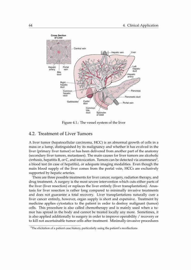
64 4. Clinical Application

Figure 4.1.: The vessel system of the liver

4.2. Treatment of Liver Tumors

A liver tumor (hepatocellular carcinoma, HCC) is an abnormal growth of cells in amass or a lump, distinguished by its malignancy and whether it has evolved in theliver (primary liver tumor) or has been delivered from another part of the anatomy(secondary liver tumors, metastases). The main causes for liver tumors are alcoholiccirrhosis, hepatitis B, or C, and intoxication. Tumors can be detected via anamneses2,a blood test (in case of hepatitis), or adequate imaging modalities. Even though themain blood supply of the liver comes from the portal vein, HCCs are exclusivelysupported by hepatic arteries.

There are three possible treatments for liver cancer, surgery, radiation therapy, anddrug treatment. A surgery is the most severe intervention which cuts either parts ofthe liver (liver resection) or replaces the liver entirely (liver transplantation). Anas-tasis for liver resection is rather long compared to minimally invasive treatmentsand does not guarantee a total recovery. Liver transplantations naturally cure aliver cancer entirely, however, organ supply is short and expensive. Treatment bymedicine applies cytostatica to the patient in order to destroy malignant (tumor)cells. This procedure is also called chemotherapy and is mainly used when a tu-mor has spread in the body and cannot be treated locally any more. Sometimes, itis also applied additionally to surgery in order to improve operability / recovery orto kill not ascertainable tumor cells after treatment. Minimally-invasive procedures

2The elicitation of a patient case history, particularly using the patient’s recollections

4.2. Treatment of Liver Tumors 65

for liver treatments are used more frequently in hospitals nowadays since they canbe performed almost ambulantly. Typically, only small incisions are made, instru-ments are injected therein, and guided to the region of interest where the therapy iscarried out. The guidance is monitored by appropriate imaging devices (for exampleC-arms). Minimally-invasive treatments are not as demanding to the patient’s healthcompared to conventional methods. However, they are seldomly used to fully curepatients from liver carcinomas but instead to relieve patients from pain and improvetheir quality of life (palliative therapy).

One such minimally-invasive treatment, which is carried out on a regular basis (5-10 times per week) in hospitals is a Transarterial Chemoembolization (TACE). Here,in order to apply local chemotherapy and embolizing the blood vessels supportingthe tumor, a catheter is inserted into the arterial vasculature in the hip region andguided to the tumor’s location using X-ray imaging (see fig. 4.2). Since the emboliz-ing liquid dissolves after a few days, this treatment is repeated on a regular basis forone patient.

Figure 4.2.: A transarterial chemoembolization. With courtesy of Dr. Jeff Geschwind,Johns Hopkins University

In the following, we will have a look at work- and dataflow of the TACE proce-dure, and deduce the necessity for 2D-3D registration from it.

66 4. Clinical Application

4.3. Workflow of Transarterial Chemoembolizations

Once a tumor has been detected and the patient is scheduled for TACE, a preoper-ative 3D scan is performed one day before the treatment. This scan is usually ac-quired via CTA or MRA and gives information about the location of the tumor, theconfiguration of blood vessels that a catheter must be guided through, and possiblecomplications due to medications the patient has received so far.

Once the procedure has been planned and the patient is accepted for treatment,TACE is started by injecting a catheter into the femoral artery of a patient who is notor only partially anesthetized. From then on, a C-arm is used to monitor the catheteras it is guided through the arterial system. Usually, a DSA is acquired providing avascular overview once the catheter has reached the aorta (see Figure 4.3a). Then, it isguided via constant fluoroscopy imaging into the hepatic artery. DSAs are frequentlyacquired to find the location of the tumor (Figure 4.3b). The catheter is led to theartery supporting the tumor (Figure 4.3c), cytostatica are applied, and the vessel isembolized.

(a) (b) (c)

Figure 4.3.: A chemoembolization workflow shown by different X-ray projections.(a) shows an overview of the vessel anatomy. The red arrow indicates the hepaticartery. (b) shows a state where the catheter is inside the hepatic arterial system. Thered arrow indicates the tumor region. (c) shows a fluoroscopy image of the statewhere the catheter has reached the tumor region.

Only a DSA where the catheter is near enough to the tumor region can visualizethe HCC. As can be seen in Figure 4.3, the overview DSA does not show the tumor.Moreover, the fluoroscopic image does not show vessels at all or only temporarily ifcontrast agent is administered. Note also that the fluoroscopic images are acquiredfrom one view only.

Currently, the 3D preoperative information is not brought to the interventionalroom. It would, however, be beneficial for the operating physician to know the posi-tion of the catheter in 3D with respect to vessels and tumor. Interventionalists oftenhave to change the angulation of the C-arm to have a better depth perception, which

4.4. Feasibility of 2D-3D Registration 67

could be avoided if preoperative data is fused with the 2D projection. As alreadymentioned in the introduction the issues of blind navigation, reduced depth percep-tion, and patient motion could be addressed if a 2D-3D registration is available andcatheter information is transferred to the 3D preoperative data set.

Even though the goal of this thesis is to provide accurate and robust methods for2D-3D registration in this context, the task of information fusion of intraoperativeinstruments and preoperative data needs to address more issues. First, in order tokeep the registration updated while fluoroscopic images are acquired and the pa-tient keeps on breathing, a tracking algorithm has to be developed compensating forbreathing movement. Moreover, the instrument, i.e. the catheter has to be located(or at least its tip) to have the 2D coordinates for backprojection into space. Last butnot least, a suitable visualization technique for data fusion must be provided, givingthe interventionalist an intuitive interface for catheter navigation.

After the presentation of 2D-3D angiographic registration techniques aligning pre-and intraoperative data sets, we will address the three aforementioned issues in theConclusion of this thesis, in chapter 7.

4.4. Feasibility of 2D-3D Registration

In the following, the problem will be analyzed with respect to the available data.Only if similar structures can be found in 2D and 3D data set a registration can be ac-complished. Moreover, we discuss the particular difficulties when registering TACEdata. Finally, we will reiterate over all the reviewed registration methods and evalu-ate their applicability to 2D-3D registration on TACE images.

4.4.1. Data Availability

Preoperative Data The current workflow for chemoembolizations in our partnerclinic involves a three-phase CTA scan of the liver region consisting of native, ar-terial dominant, and portal-venous phase visualizing especially the portal venoussystem, faintly the arteries, and the hepatic veins. The native scan is done to detectalready existing embolization liquid in the liver. The arterial dominant phase allowsfor detection of new malignancies, and, together with the venous phase, shows theradiologist whether a treatment is possible with the current vessel configuration.

During the intervention, however, only arteries are visible in the 2D data sets, noportal or hepatic vessel systems, such that until now 2D-3D registration was notpossible. We create a strong link between diagnostic radiology and intervention bydefining a new protocol for the preoperative scans, introducing one additional run ofan angiographic phase that visualizes liver arteries (delay times with bolus tracking:6 (angiographic), 10 ± 2 (arterial dominant), 21 ± 4 (portal-venous) seconds), seeFigure 4.4. The aim is to let the interventionalist benefit from 3D high resolutionCTA scans during the intervention. We have acquired several data sets using a state-of-the-art 64-slice CT imaging device (Siemens Sensation 64). The spatial precisionof the acquired scans could be reconstructed to 0.58 × 0.58 × 0.6 mm3/voxel in a

68 4. Clinical Application

512 × 512 × (280 − 500) voxel volume making it possible to extract vessels with adiameter down to 1− 2mm.

As confirmed by physicians, the additional radiation exposure (approximately 6mGy) is acceptable for patients undergoing a chemoembolization treatment. Thisnew scan protocol is used to perform the registration. As a result, path planning canbe performed and intraoperative 3D visualization can be offered.

(a) native (b) angiographic (c) arterial dominant (d) portal-venous

Figure 4.4.: The new 4-phase CT protocol

Intraoperative Data We choose to register the preoperative data set to a DSA. Flu-oroscopic images show bone structure, which could be used for rigid registration.However, the structure to be aligned is the vessel system that is subject to motion(rigid and non-rigid), which cannot be inferred from the skeletal structure3. Thus,a registration algorithm should focus on the structure of interest, the vasculature,supporting the use of DSAs. Moreover, for feature-based registration algorithms,an extraction of vessel features is necessary, which can be accomplished easier us-ing DSAs compared to contrasted fluoroscopic images due to a better signal-to-noiseratio and less artifacts.

4.4.2. Challenges

Even though the preoperative acquisition is altered to provide necessary informationcommon to both pre- and intraoperative data set, there are still some challenges thathave to be coped with.

Contrast Difference First, contrast injection is performed globally for the preoper-ative, locally for the intraoperative data set. Thus, contrast propagation stops earlierin the vessel structure in preoperative data, while thinner vessels are visible in intra-operative data. A registration based on vessel structures has to discard those outliersin the 2D data set. Moreover, possible segmentation errors as well as the global con-trast propagation can introduce vascular outliers in 3D, too.

3Breathing motion, for instance, induces different transformations on organs (and thus vessels), ribs,or spine

4.4. Feasibility of 2D-3D Registration 69

Small Vessels As already mentioned in 4.1, hepatic arteries have a diameter of1− 5mm making it difficult to provide a proper segmentation. Particularly in a pre-operative CTA small arteries shrink to the size of one voxel only, making segmen-tations prone to errors caused by noise. These segmentation errors either have tobe compensated by a suitable vessel extraction algorithm, or have to be consideredduring 2D-3D registration.

Breathing Movement Due to patient breathing the vessel structures are deformed[151, 125]. Either the deformation is taken into account by the transformation model,or deformed vessels have to be detected and discarded for a rigid registration method.Moreover, a DSA usually shows artifacts (a displaced catheter or rib contours, seeFigure 4.3), which have to be taken into account during registration. A 2D segmen-tation algorithm has to be robust against such artifacts, and a 2D-3D registrationbased on intensities must not be disturbed by them.

Single View Our clinical partners only use a single view C-arm for TACE treatmentas do most other hospitals for abdominal catheterizations. Thus, no 3D reconstruc-tion and 3D-3D registration approach is possible in this specific scenario. The depthinformation has to be inferred from one view only, making a deformable alignmentparticularly difficult, see 3.4.

Fast and Automatic A registration algorithm must be fast and automatic since itwill be used during the intervention. While preoperative data can be (semi-)manuallysegmented, the 2D vessel extraction should be as automatic as possible, or the reg-istration has to be computed without 2D segmentation. Moreover, a registrationshould not require a manual pre-alignment, proper initialization routines have to beprovided for applicability.

4.4.3. State-of-the-Art Applicability to TACE

We will now highlight advantages and flaws of approaches already proposed in theliterature, and discuss their applicability to TACE data.

Feature- vs. Intensity-Based Registration Pure intensity-based registration for an-giographic alignment of TACE data is rather difficult to achieve. First, most of theintensity-based approaches that have been reviewed above need a segmentation ofthe 3D vasculature, which makes it unreasonable to not at least use attributes likediameter and centerline of the preoperative data set. The methods based on MIPapproximations of DRRs are not likely to work due to the small nature of hepatic ar-teries. A MIP of the arterial vascular system of the liver will be prone to error due tonoise and alignment might fail especially if the depth information gathered duringMIP is used in the registration process as proposed by Kerrien et al. [73].

70 4. Clinical Application

Deformation and Size Bias of Intensity-Based Methods Liver arteries deformduring patient breathing. Unfortunately, it can occur that also thick vessels deformvastly (see chapter 6), which makes it difficult to align the images according to them.Methods based on intensity similarity measures tend to align vasculature biased bythe diameter of the vessels. The larger the vessel, the more influence it gains in thesimilarity measure. However, due to non-rigid motion, vessels with different sizesshould rather be treated equally in order to attain more robustness against deforma-tion. This makes a registration using the methods of Hipwell [68, 101, 23], Day andNapel [39], Turgeon [145], or Chan [27] difficult in abdominal regions.

Furthermore, we find it also crucial for a registration algorithm to have informa-tion about 2D vessel geometry, topology, and diameter properties. In this respect,2D vascular segmentation is an important step in our opinion, and we will show inchapter 5 that a mere normalization of vessel radius and an avoidance of 2D segmen-tation as proposed by Jomier et al. [70] is not sufficient for a successful registration insome clinical cases.

Automation A high level of automation must be achieved intraoperatively in orderto make the algorithm applicable for TACE procedures. A tedious manual segmen-tation of 2D data is to be avoided, which excludes some approaches (e.g. that byAlperin et al. [1], Liu et al. [88], or Vermandel et al. [150]) for 2D-3D registration usedon chemoembolization image data. Moreover, automatic initialization is an impor-tant issue and the capture range of algorithms should be high. We will propose anddiscuss suitable automatic initialization techniques to find an initial estimate in thevicinity of the true registration parameters.

Deformable Registration Non of the reviewed methods is solving for a local trans-formation acknowledging the deformation introduced by patient breathing and pres-ence and advancement of the injected catheter. It is doubtful whether the bitangentproperties derived by Feldmar et al. [41], or the region-based correspondence searchas described by Kita et al. [77] still work in this deformable environment. In the fol-lowing chapter, we will propose two rigid registration algorithms, which are bothrobust against deformation changes and solve for transformation parameters as wellas one-to-one correspondences. We link these results to a deformable 2D-3D registra-tion algorithm in chapter 6, which for the first time addresses the difficult problemof non-rigid vascular alginment of a 3D image to a single 2D projection.

5. Rigid 2D-3D Registration of Angiographic Images

This chapter introduces two methods for rigid registration of 3D CTA to 2D DSAimages of abdominal catheterizations.

In the first two sections, 5.1 and 5.2, we will provide details on the model of theC-arm we use for deducing the registration parameters and explain the preprocess-ing of the data we have to apply to retrieve the data structures that are used foralignment.

Next, the bifurcation-driven registration will be discussed in section 5.3, a methodto register two vascular graphs using bifurcation points and topological graph infor-mation to adapt 3D to 2D feature space. In section 5.4 we will introduce the secondrigid registration algorithm, in which the alignment is driven by an iterative 2D seg-mentation refining feature spaces for correspondences. Both methods will be subjectto extensive testing, and a method for creating a simulated DSA image with a groundtruth registration is developed to evaluate accuracy and robustness of the second al-gorithm since it is using 2D image intensities in the registration process.

Integrating the registration results into clinical workflow will be postponed tochapter 7. Registration-induced visualization and a subsequent catheter trackingmethod will be discussed there.

5.1. C-arm Model

The presented model interprets the calibration matrix K and extrinsic parameters[R|t] of a pinhole projection in the context of a C-arm setup. For an illustration referto Figure 5.1. All images were acquired with C-arms of the Axiom series of SiemensMedical Solutions.

Intrinsic Parameters We assume an absence of distortion due to flat panel detec-tor technology or correction by calibration. The intrinsic parameters can be receivedfrom the calibration given by stationary C-arms for reconstruction purposes (or in-terpolated from them as explained in 2.4.2).

The focal length fx, fy is given in mm by a calibrated field of view (FOV ), imagewidth hx and height hy, aspect ratio a, and the pixel pitch mx, my:

fx = mxhx/2

a tanFOV/2, fy = my

hy/2tanFOV/2

(5.1)

The principal point (px, py) is either given by calibration, or, if not available, anapproximative value is given by the center of the image (hx/2, hy/2).

72 5. Rigid 2D-3D Registration of Angiographic Images

Figure 5.1.: 6 rigid body parameters in a C-arm setup

Extrinsic Parameters The origin of the WCS (center of rotation) is placed in themiddle of the moving 3D image, where a right-handed coordinate system spans aplane by x− and y−axis parallel to the image plane. Moreover, the WCS originis located on the ray connecting CCS origin and principal point, making the z-axislie on the principal ray. Since C-arm geometry places the 3D object between X-raysource and image plane, the following interpretation of the 6 rigid-body parameterscan be deduced:

• α: rotation around horizontal axis of image, secondary angle of C-arm

• β: rotation around vertical axis of image, primary angle of C-arm

• γ: rotation around principal ray

• tx: in-plane translation along horizontal axis of image, perpendicular table trans-lation

• ty: in-plane translation along vertical axis of image, parallel table translation

• tz : out-of-plane translation along the principal ray, table translation towards X-ray source or detector

The rotation matrix R is then given by the matrix representation of the Euler angles(α, β, γ), and the translation t = (tx, ty, tz)�.

5.2. Preprocessing 73

5.2. Preprocessing

For all proposed methods, we developed a graph representation of centerlines andbifurcations of vessel structures attributed with the diameter at each location. Theprocess is divided up into three stages: the vascular segmentation (section 5.2.1), theextraction of centerlines, bifurcations, and diameters (section 5.2.2), and the creationof the graph structure (section 5.2.3). A visual overview of all steps is given in Figure5.2.

5.2.1. Segmentation

CTA Segmentation Since contrast agent is applied globally in a CTA scan, its prop-agation is uniform and rather straightforward to segment. Thus, we choose a regiongrowing algorithm to extract the vascular structure, as described in 2.2.4. In order toavoid the region growing to stop due to noise, a smoothing is applied. The smooth-ing has to be edge-preserving since small vessels are important to be covered by thealgorithm and leakages due to low contrast difference should be avoided. Therefore,the 3D volume of the angiographic scan is filtered with anisotropic diffusion [119]before the user has to place a seed point at the beginning of the arterial tree to besegmented.

The angiographic phase of CTA shows contrasted aorta and the arterial system ofother organs than the liver, too. The user manually selects a point in the vicinity ofthe hepatic artery where it leaves the aorta. By automatically drawing a cube withthe size of the hepatic artery, the region growing is stopped and redundant vascularinformation that is not visible in the intraoperative image can be discarded.

As can be seen in Figure 5.2b this segmentation technique yields good results forthe extraction of hepatic arteries from the angiographic CTA scan. However, as wasassessed manually, very small vessel structures cannot be segmented using a regiongrowing due to noise. Level Set methods (see 2.2.4) could provide a better segmen-tation in terms of vessels with a diameter of less than two pixels. However, we pre-ferred the region growing technique since it provides reasonable results for 2D-3Dregistration, is computationally fast, easy to implement, and the segmentation canconveniently be refined manually.

DSA Segmentation In 2D DSAs, the SNR is higher compared to 3D CTAs, makingit necessary to use a more sophisticated vessel enhancement filter. A backgroundremoval is performed by applying a bothat filter (closed image minus original im-age) followed by a multiscale vesselness filter assigning the probability of lying ina tubular structure to each pixel as described by Frangi et al. [47]. Again, a regiongrowing algorithm extracts the vessel structure from one or several seed points.

5.2.2. Extraction of Graphs

From the segmented data sets one can easily extract a centerline image by applyingtopology-preserving thinning algorithms in 3D and 2D [113]. A wave propagation

74 5. Rigid 2D-3D Registration of Angiographic Images

algorithm [162] extended to cope with loops is used to create a graph from this cen-terline [112]. By advancing a set of waves and testing their fronts for connectivity,a graph can be created with bifurcation nodes at branching points of the vessel treeand segments consisting of sampling nodes in between (see Figure 5.2). Mind thatthe position of ramification points is directly depending on the thinning algorithm.Since thinning is an approximation to MAT [14], the (unique) bifurcation lies on thecenter of the largest sphere that can be fitted into the segmented vasculature.

(a) original CTA (b) segmented CTA (c) extracted 3D graph

(d) original DSA (e) segmented DSA (f) extracted 2D graph

Figure 5.2.: Preprocessing in 3D/2D. Figure (a) shows the volume rendered CTA,(b) shows the segmented vasculature, (c) the extracted graph, where the greenpoint is the root node, orange points inner, red points outer bifurcation points, andblue points represent sampling points of the vessel segments. Figure (d) and (e)show original DSA and its segmented vasculature. Figure (f) shows the 2D graph(turquoise are sampling, red are bifurcation points)

Points between each bifurcation are sampled and stored as edge labels to keepedge position information. The size of a wave should be set to the desired samplingrate of segmented vessels, which can be down to 1 pixel or voxel. Note that a ves-sel graph in 3D is not necessarily a tree since there can be anatomical loops in thevasculature as has been confirmed by physicians. Since the thinning algorithm stillintroduces some wrong branches due to noise, edges smaller than the vessel diame-

5.2. Preprocessing 75

(a)

Figure 5.3.: Illustration of the used graph structure.

ter are removed with a Euclidean distance map of the segmented data sets. For thesame reason and in the same way very adjacent bifurcations are fused together.

The diameter of the vessels is computed using a distance map of the segmentedimage. The distance map is created such that the largest Euclidean distance to thecontour is given inside the segmentation. On each centerline point, the radius, andhence the diameter can be determined thus, as described in section 2.2.5.

5.2.3. Graph Representation of Vessel Centerlines

We model vessel structures as directed graphs Gd = (V d, Ed), with a set of n nodesV d ⊂ R

d and the connecting edges Ed ⊂ V d × V d. Here d ∈ {2, 3} denotes thedimension of the graph. For the following, please refer also to Figure 5.3.

The nodes are classified either as bifurcation nodes V db or sampling nodes V d

s , suchthat V d = V d

b ∪ V ds and ∅ = V d

b ∩ V ds . While the bifurcation nodes express the topol-

ogy and the rough geometry of the vessel tree, the sampling nodes are used to de-scribe the geometry of the vessel segments in more detail.

A general graph node is abbreviated by V ∈ V 3, and v ∈ V 2, in order to distin-guish between the two dimensions we are working on.

The bifurcation nodes are abbreviated by B in 3D and b in 2D and are identifiedwith their spatial coordinates, such that B ∈ V 3

b ,b ∈ V 2b .

We denote the sampling nodes by X in 3D and x in 2D and again identify themwith their spatial coordinates.

We define a vessel segment Πi,j as a path between two neighboring bifurcationnodes Bi and Bj , containing all sampling nodes and edges between Bi and Bj . Thenumber of nodes in Πi,j is ni,j and the number of edges respectively ni,j + 1. The

76 5. Rigid 2D-3D Registration of Angiographic Images

sampling nodes are indexed relative to the vessel segment Πi,j starting from 1 to ni,j ,compare Figure 5.3. The correspondences are also ordered relative to the respectivevessel segment.

We will also use a topological version of a graph Gt = (V t, Et), where V t = V db are

only bifurcation nodes, and Et ⊂ V db × V d

b represents the ramification topology ofthe vessel structure.

5.3. Bifurcation-Driven 2D-3D Registration

Given 2D and 3D graphs from the newly introduced angiographic CTA scan and theDSA image, the aim is now to recover the 6 extrinsic parameters to form [R|t]. Thisis an easy task if correspondences are given, in our scenario, however, correspondinginformation is not available and has to be determined as well.

In the following method we use the fact that bifurcation locations are distinct, andwell-defined. Moreover, bifurcations form a space of correspondences between 2Dand 3D graph structure. In a first step, the algorithm is initialized by finding onebifurcation correspondence via a-priori information of the patient location and iter-ative (x, y)-translation. Fixing this correspondence, a nonlinear optimization is per-formed on a reduced parameter space iterating over 3 rotational and 1 translationalparameter. Good feature correspondences are iteratively created for the matching byrecurrent graph creation of the projected 3D centerline image.

5.3.1. Initialization

State-of-the-art angiographic C-arm devices store lots of information concerning imag-ing geometry. Each 2D angiogram is provided with the calibration matrix K, and asource-to-table distance (STD, see Figure 5.1). Moreover, a primary and secondaryangle provide a good initial estimate of the rotation matrix R.We use all this information to produce initial image as well as object coordinates ofthe extracted vessel trees. For all node coordinates of the 2D centerline graph vi weundo the transformation specific to the imaging device:

vi = K−1 ˜vi (5.2)

For all node coordinates of the 3D centerline graph Vi, we apply an initial transfor-mation including primary and secondary angle R (assuming γ = 0) and an approxi-mate z-translation tz = (0, 0, STD)�:

Vi = ViR + tz (5.3)

Naturally, the values of rotation parameters and z-translation are just a rough esti-mate and subject to further optimization as described in the following section.

Registration of x-y-Translation This step tries to find a 2D correspondence to thebifurcation in 3D with the largest vessel attached, which is called the root. After

5.3. Bifurcation-Driven 2D-3D Registration 77

setting the a-priori information, we iteratively translate the 3D graph in x- and y-direction parallel to the image plane such that the root’s projection is laid over 2Dbifurcations with high diameter. The energy Etopo, described in Equation (5.7), isevaluated and the (x, y)-translation yielding the lowest value is chosen. Thus, wefind one corresponding vertex and reduce our optimization problem to recoveringthree rotational parameters (R) and one translational parameter tz along the ray con-necting the X-ray source position to the projected root on the image plane.

5.3.2. 4 DOF Optimization

Geometric Optimization of Rotation and z-Translation 2D-3D registration prob-lems are twofold: recovery of corresponding information and estimation of rigidtransformation. Since vessel structures can be interpreted as a set of curves, the Iter-ative Closest Point (ICP) algorithm [163, 11] could be incorporated for finding both,matches and transformation parameters. Let C(G,y) be a function determining thepoint of graph G closest to a given point y, an energy Eicp can be defined by

Eicp =n2�

i

||C(G2D, f[R|tz ](Vi))− f[R|tz ](Vi)||2, (5.4)

where G2D is the 2D vessel graph, Vj , j = 1 . . . n2 are all points representing the 3Dvasculature (bifurcations and segment sampling points). With tz = [tx, ty, tz]� weindicate that only tz is subject to optimization, tx,ty are fixed.Eicp has many local minima since projected points of one 3D vessel segment could

easily be driven to different, not corresponding 2D vessel segments in the optimiza-tion process. Moreover, even with outlier detection via an adaptive distance thresh-old based on statistical analysis [163], the energy would yield wrong alignment dueto deformation.

If we do not focus the correspondence search on all curve points but only on dedi-cated ones that are likely to be detected in both data sets, we can improve the estima-tion process. Bifurcation points can be detected in 2D and 3D data sets very easilyand represent good descriptors for a projection of vasculature since they are dis-tributed over the whole vessel tree and are distinct to each other. Hence, we restrictour energy only to these good features, the ramifications of the vessel graphs:

Ebif =n3�

i

||C({bj}, f[R|tz ](Bi))− f[R|tz ](Bi)||2, (5.5)

where b1, . . . ,bn2D and B1, . . . ,Bn3 are bifurcation points of the 2D and 3D graphs,respectively. Only inner bifurcations can be used since leaves in the graph accountfor the end of contrast propagation, which is different in 3D and 2D data set.

Unfortunately, segmentations and hence extracted graphs of the data sets are of-ten very different due to local and global application of contrast agent. Moreover,the projection also produces crossings of vessels that cannot easily be detected andresolved since vessels can also be tangent to each other. This can be dealt with byperforming a new graph extraction on the projected graph’s centerline image in each

78 5. Rigid 2D-3D Registration of Angiographic Images

iteration (see fig. 5.4). The centerline image is created by drawing the 3D graph asa one-voxel-wide centerline in a volume and projecting the volume with the currentimaging parameters. The new energy can be stated now as

Eextract =n4�

i

||C({bj},bfi ))− bf

i ||2, (5.6)

where {bf1 , . . . ,bf

n4} is the inner bifurcation list (without leaves) of a graph, which is

created as follows:

• From 3D graph G3D a centerline volume A is created.

• A is projected with projection function f[R|tz ] to yield a centerline image Af .

• A new graph Gf is extracted from the projected graph’s centerline image Af

starting at the location of the projected root vertex.

• Only the inner bifurcations of Gf are put into the resulting set {bf1 , . . . ,bf

n4}

(a) (b) (c)

Figure 5.4.: Fig. (a) shows the real 2D graph, (b) the projected 3D graph, and (c)the new created graph from the centerline image of the projected 3D graph. Thewhite arrows show the bifurcations in 2D that are not present in fig. (b), but couldbe detected by the wave propagation, see fig. (c).

Topological Optimization of Rotation and z-Translation Since we deal with graphstructures, we can also incorporate topological information in the registration. Dueto different segmentation results in 2D and 3D, the two graphs to be registered donot fulfill the subgraph property and it is not straightforward to do a topology-basedgraph matching to register the data. However, topological tendencies can be used forregistration. The degree of each vertex can be used as well as a time stamp comingfrom a breadth first search to penalize wrong bifurcation matches:

Etopo =n�

i

rbi r

di ||C(bj ,b

fi )− bf

i ||2, (5.7)

5.3. Bifurcation-Driven 2D-3D Registration 79

where rbi is the ratio of the normalized breadth first search values of the current

bifurcation bfi and the closest bifurcation in the 2D graph or its reciprocal if rb

i < 1.rdi is the ratio of the degrees of bf

i and the closest 2D bifurcation or its reciprocal ifrdi < 1. Graph searches and degrees are computed on the topological representation

of the respective graphs (see 5.2.3).

Optimization Scheme Due to the high non-linearity of the cost function Etopo agradient-based optimizer is not used. In each iteration the graph creation changesthe number of possible correspondences and the scope of the squared sum differs,hampering the derivation of a valid Jacobian. Therefore, instead of using gradient-based methods, the downhill simplex [123] algorithm was favored.

5.3.3. Algorithm Evaluation

Creation of Reference Registration Experiments have been carried out on syn-thetic data from 3D head vasculature, a phantom head showing a rigid vessel struc-ture, and on four patient data sets of TACE procedures. For creating (rigid) syntheticground truth data, we extracted the 3D centerline from the head phantom and pro-jected the resulting graph with rotation and translation typical to a patient-C-armsetup. The transformation was chosen to produce a projection with a similar numberof overlays that could be found in real data sets. For the phantom head, a referenceregistration has been created by intensity-based registration using Gradient Correla-tion [118] as similarity measure (see Figure 5.5). For the patient data sets a manualregistration was provided by experienced radiologists.

(a) (b) (c)

Figure 5.5.: Fig. (a) shows a volume rendering of a 3D head phantom, fig. (b) anX-ray projection of this head. Fig. (c) shows a checkerboard image of inverted 2Dand DRR of the reference registration.

Accuracy Measure For accuracy assessment, we used the RSME measure of Equa-tion (2.43), defined between the reference registration parameters and the computed

80 5. Rigid 2D-3D Registration of Angiographic Images

parameters. In the robustness tests, the standard deviation was also computed inorder to account for the stability of the error.

Robustness Test In order to evaluate the convergence and robustness of the op-timization, Monte Carlo simulations have been carried out on all data sets. Ran-dom displacements in a range of ±10mm in translation along the axis connectingX-ray source position to root node (tz) and ±10◦ in rotation angles (α, β, γ) havebeen added to the reference pose and the registration procedure was invoked. Thesedisplacements are equivalent to a range of 10-50 mm average projection distance ofbifurcation points. Note that in order to have the same 3D displacements on all datasets a transformation has to be applied to all coordinates of G3D before the tests, suchthat the WCS origin is located in the center of the volume (which equals the centerof rotation).

The algorithm has been invoked from a total of 200 randomly generated simula-tion poses.

Method Comparison Moreover, we implemented the method of Jomier et al. [70]and added errors of up to ±10mm and ±10◦. For the realization of Jomier’s method,instead of the 1D parameter search as proposed in the original paper, we used aDownhill Simplex optimizer to solve for 6 DOF minimizing the cost function as de-fined in Equation 3.8. We performed a second test with smaller errors (up to ±5 mmand±5◦, equal to 5-25 mm average projection distance of bifurcation points) becauseJomier’s method solves for all 6 DOF, not only 4.

Results Tables 5.1 and 5.2 show standard deviations and root mean square errorsof 200 trials for the 6 degrees of freedom (3 translation and 3 rotation parameters).Rows denoted with M1 refer to results from our method, those with M2 10 showresults from Jomier’s algorithm with the large error range, those with M2 5 with thesmall error range.

We did not perform tests for Jomier’s method on synthetic and rigid phantomdata since no image intensities were created in the former, and no DSA image (onlya fluoroscopic image) was available in the latter case, respectively. Our method issometimes outperformed in z-translation (tz), which is the translation perpendicularto the image plane. These deviations, however, do not create a large pixel error whenprojected (about 3 mm average projection distance of bifurcation points). The moreimportant rotation angles and in-plane translation values prove to be more accuratewhen using our method. Figure 5.6 shows three patient data sets after initializa-tion (a),(b),(c) and after optimization (d),(e),(f). The blue line shows the extracted 2Dgraph, and the green line the projected 3D graph. As can be observed, the optimiza-tion procedure improves the initial alignment up to a deformation of the vessels.

Runtime Finding one correspondence and thus two parameters, tx and ty, wassuccessfully performed for each of the data sets. It took between 0.5 and 1.8 seconds

5.3. Bifurcation-Driven 2D-3D Registration 81

(a) init Patient 1 (b) init Patient 2 (c) init Patient 3

(d) optimized Patient 1 (e) optimized Patient 2 (f) optimized Patient 3

Figure 5.6.: Initialized and registered pose of three patient data sets.

on a 1.6 GHz Pentium machine. The optimization procedure took 2.5 - 6 seconds forphantom and patient data.

5.3.4. Discussion

By developing a 2D-3D registration algorithm based on the newly acquired data, weenable physicians to transfer planning information to the interventional room, andvisualize patient anatomy in 3D from the same view point (see 7.1.1). We overcomethe difficulty of alignment by conceiving an algorithm, which iteratively generatesgood features that can be detected easily in 2D and 3D and describe the perspec-tive projection adequately. The algorithm requires user interaction for 3D and 2Dsegmentation. Since the preoperative 3D segmentation is not subject to hard timeconstraints, the vasculature extracted by region growing can be refined several timesand tailored to thoroughly represent the hepatic arterial system. The intraoperativesituation does not allow an extensive user interaction, so we provide a single clicktechnique to start a region growing on a restrospectively enhanced DSA image. Dueto the small amount of user influence, the segmentation in 2D is suboptimal, whichwe account for with a restriction of the registration to bifurcation points only, re-ducing the number of outliers extensively. With this technique, we also address theinherent difference of vascular images due to global and local contrast injection.

82 5. Rigid 2D-3D Registration of Angiographic Images

Data Method σtx σty σtz σα σβ σγ

head simulation M1 0.0004 0.0005 0.0050 0.0028 0.0010 0.0026M2 - - - - - -

head phantom M1 0.0005 0.0005 0.0069 0.0019 0.0009 0.0022M2 - - - - - -

patient 1 M1 1.3487 1.3982 48.5488 6.2751 2.4778 0.9400M2 10 17.9463 43.9687 18.8130 19.8789 19.0780 17.4332M2 5 11.9465 35.8826 11.7423 7.9779 11.3076 9.9759

patient 2 M1 0.1463 1.2696 5.0197 4.5966 2.5925 1.2467M2 10 2.6396 2.9281 8.0932 7.9089 6.5415 2.0341M2 5 1.0204 1.2284 5.5270 5.3732 4.6572 0.6931

patient 3 M1 2.7590 7.5364 45.0523 7.7809 3.9825 7.3726M2 10 20.7737 45.7128 16.5745 11.7821 17.2824 21.9335M2 5 19.1786 11.3295 8.7508 6.0658 9.9346 4.1008

patient 4 M1 6.9731 1.3264 64.3743 6.3780 8.0713 4.3081M2 10 43.3558 13.6386 16.8588 20.1722 24.1609 21.4028M2 5 18.4730 5.5094 11.0570 6.7126 20.7805 6.2196

Table 5.1.: Standard Deviations (σ) of Rigid Registration of 200 Monte Carlo simula-tions in mm for tx, ty, tz and degree for α, β, γ, respectively

Data Method RMStx RMSty RMStz RMSα RMSβ RMSγ

head simulation M1 0.0389 0.2689 2.2302 0.3966 0.0014 0.5100M2 - - - - - -

head phantom M1 0.1104 0.1787 1.2799 0.5842 0.0291 0.6455M2 - - - - - -

patient 1 M1 1.3815 1.4114 56.2447 6.8791 3.6151 0.9527M2 10 22.3263 58.1284 19.6391 19.8301 21.5437 21.6254M2 5 13.2387 40.4219 12.8111 7.9678 12.7487 11.5099

patient 2 M1 1.2302 1.4209 28.4073 5.0616 3.8540 2.3298M2 10 2.6345 4.1985 8.0793 8.9258 6.6079 2.1112M2 5 1.0380 2.8683 5.5190 6.1704 4.6732 0.7196

patient 3 M1 6.5579 7.8977 66.3731 7.9441 11.8805 7.4747M2 10 20.7272 61.2542 17.9872 14.4016 19.0442 29.2579M2 5 19.3971 11.3037 9.2925 6.2510 15.4947 4.3602

patient 4 M1 10.6187 2.1967 88.9475 8.4271 16.2405 5.5228M2 10 49.3440 14.5086 17.0029 21.6873 25.1797 22.1071M2 5 19.1812 5.7051 11.2161 7.3732 21.6268 6.3191

Table 5.2.: Root Mean Square Errors (RMS) of Rigid Registration of 200 Monte Carlosimulations in mm for tx, ty, tz and degree for α, β, γ, respectively

5.4. Segmentation-Driven 2D-3D Registration

The bifurcation-driven registration process has performed satisfactory in many clin-ical cases. However, we have found out that some data sets of liver arteries do notshow enough bifurcations (even with the detection of projected bifurcations) to drivethe registration to the desired solution, especially when the patient has undergoneseveral treatments already. Thus, we would like to incorporate the full informationof vessel segments for registration, not only junction points. Moreover, the user in-teraction required during intervention is not desirable since time is a critical factor.

We developed an alternative method, which is fully automatic during the inter-

5.4. Segmentation-Driven 2D-3D Registration 83

vention and yields good results even if only a small part of the vessel tree is visibleor many outliers are present. By coupling a technique for automatic seed point de-tection developed by Can et al. (see 2.2.3) for 2D vascular structures with a regiongrowing step, we avoid user interaction intraoperatively. A combination of registra-tion and 2D segmentation via a probability map allows us to adjust the feature spacessuch that non-corresponding features in 2D as well as 3D vasculature are removedconsequently while the full vessel curve information can still be used for alignment.

With this approach we combine robustness and high capture range with a fullyautomatic registration technique. Moreover, one-to-one correspondence of vascularfeatures is assured, which makes it possible to visualize roadmaps in 3D as discussedin chapter 7.

We motivate our method through a maximum likelihood (ML) formulation solvingfor both registration and segmentation. Unlike other algorithms for combined seg-mentation/registration, we only care about the resulting registration and also leavethe algorithm as generic as possible in order to use alternative registration and seg-mentation steps. In section 5.4.2 we apply our algorithm to 2D-3D DSA-to-CTA reg-istration for abdominal interventions.

Related Work to Combined Segmentation / 2D-3D Registration A combinationof segmentation and 2D-3D registration was proposed by Hamadeh et al. [64] andBansal et al. [7] for the rigid alignment of medical images. The former only seg-mented once for aiding the registration, the latter used a minimax-approach in orderto optimize one energy functional that encapsulates the joint conditional entropy ofDRR and X-ray given a segmentation. A recent method proposed by Brox et al. [20]combines pose estimation with a level set formulation to let a registration aid the seg-mentation. In all these methods, the segmentation is integrated into the algorithmand cannot be replaced. Since vessel segmentation is a specific problem where gen-eral approaches cannot be applied without modification we tried to leave the combi-nation as generic as possible and discarded these methods. Combined segmentationand registration has also been successfully applied to brain MR images (see Pohl etal. [122] and references therein) where an Expectation Maximization (EM) formula-tion was favored. In contrast to our proposed algorithm, this work also solves forMR specific nuisance parameters and serves a diagnostic application not subject tohard time constraints.

5.4.1. MLE with Labelmaps

In the following, we will denote the model of a vessel graph G by M. M is aninstantiation of a random variable M , where all node coordinates of G are stackedup. M does not own diameter or topological information. We will treat an image I asan instantiation of a random variable I with intensity values as entries. A labelmap(segmentation) is expressed as L. A labelmap of size n× n is built from n2 indicatorlabels �x. Probabilities of a random vector X will be denoted by P (X ).

We want to maximize the probability that certain registration parameters Θ fit best

84 5. Rigid 2D-3D Registration of Angiographic Images

the 3D modelM to the 2D image data I, i.e. we want to find a maximal probability

P (Θ|I,M) =

likelihood� �� �P (I,M|Θ)

a priori� �� �P (Θ)

P (I,M)� �� �normalizing constant

.(5.8)

Thus, the Maximum Likelihood estimation (MLE) of the registration is

Θ = arg maxΘ

P (I,M|Θ). (5.9)

Maximizing the likelihood of Equation (5.9) is very difficult if there is no corre-spondence information between image pixels and model points. Thus, we let a 2Dsegmentation aid the estimation. We introduce a random variable L representing alabelmap over the image I. Marginalizing over Lwe get

Θ = arg maxΘ

�L

P (Θ,L|I,M) (5.10)

= arg maxΘ

�L

P (L|I,M)P (Θ|L, I,M) (5.11)

using the product rule. From this formulation we can deduce an iterative scheme. Ifwe had values for variable L given, we could solve the ML of Equation (5.11). SinceL has to be estimated also, we iterate between expectation estimation (E-step) of theunknown random variable L and optimization of a cost function (M-step) given thisexpectation:

L(t) ← E(L|Θ(t−1), I,M) =�LLP (L|Θ(t−1), I,M) (5.12)

Θ(t) ← arg maxΘ

P (Θ|L(t), I,M)ML∝ arg max

ΘP (L(t), I,M|Θ) (5.13)

The M-step (Equation (5.13)) is rather easy to accomplish since we already have amodel in 3D (M) and can determine the MLE using L(t) in a model-to-model regis-tration, using for example an ICP algorithm.

For the E-step (Equation (5.12)), however, we must determine the expectationvalue of the labelmap given the last registration and the data. Since this is notstraight-forward, we will discuss it in more detail.

Assuming spatial independence of pixels in image I (which is common in thiscontext, see [122, 7]), we can determine the expectation for each pixel x separately. Ifwe restrict our segmentation on one object only, we can deduce an indicator variable�x for each pixel x, where

�x =�

1, if x is inside the object0, otherwise

(5.14)

Thus, the expectation for the label �x of a pixel x becomes

E(�x|Θ(t−1), I,M) = P (�x = 1|Θ(t−1), I,M) (5.15)= αP (Θ(t−1)|�x = 1, I,M)P (�x = 1|I) (5.16)

5.4. Segmentation-Driven 2D-3D Registration 85

using Bayes’ rule, where α = 1/P (Θ(t−1)|I,M), and M is dropped in the last termof (5.16) since the segmentation of I is independent of the 3D model. With Equation(5.16) we can assign the expectation of the segmentation to each pixel and thus geta probability map IL(t) for L(t). We can interpret this map as the probability for eachpixel to be registered (has a correspondence) to the model, given that it is part of thesegmented object combined with the a-priori probability to be part of the segmentedobject.

Note that we see the expectation as a probability where we joined the registrationparameters from the last iteration and the a-priori knowledge of a pixel belongingto an object. We still keep the freedom to choose any kind of binarization technique,which we apply to the probability map.

We can give a generic algorithm for the segmentation-driven 2D-3D registration,which we will henceforth refer to as EBM algorithm as summarized in Algorithm 3.

Algorithm 3 EBM: Segmentation-driven 2D-3D registration

Given image I, a model M, initial estimates of parameters Θ(0), and labelmapL(0)

Θ(t−1) ← Θ(0)

L(t−1) ← L(0)

while ¬converged doE-step: Create probability map IL(t) : For each pixel x with �x = 1 determine theprobability for the new label using Equation (5.16). For each pixel x with �x = 0 set theprobability to zero.B-step: Binarize IL(t) to get L(t).M-step: RegisterM to L(t) starting from Θ(t−1) to get Θ(t)

end while

Note that our method does not follow the strict formulation of the EM algorithm[37],

Θ(t) = arg maxΘ

�

LP (L|Θ(t−1), I,M)P (L, I,M|Θ). (5.17)

In our algorithm, we directly calculate the expectation of the hidden variable L,whereas EM calculates the expectation of the probability of the complete data (L, I,M)given the incomplete data (I,M) and an estimate of Θ. Unlike EM, convergence isnot proven for our approach. In our experiments, however, the algorithm alwaysconverged given suitable termination criteria.

5.4.2. The EBM Algorithm for Angiographic Registration

We can now apply the EBM algorithm to rigid CTA-to-DSA registration. Severalsteps of the algorithm are illustrated in Figure 5.7. Given a DSA image I (Figure5.7a) and the vasculature model M (laid over the DSA in Figure 5.7f) of a CTA vol-ume. The 3D point cloud that spatially describes M, i.e. sampling points on vessel

86 5. Rigid 2D-3D Registration of Angiographic Images

(a) (b) (c)

(d) (e) (f)

Figure 5.7.: Illustration of the segmentation-driven registration: (a) original DSA, (b)bothat filtered DSA, (c) initial segmentation (automatic seed point detection, regiongrowing), (d) probability map penalizing non-corresponding but extracted featuresin 2D and 3D, (e) final segmentation after registration - increased feature similarity,(f) overlay of 3D vasculature and DSA

centerlines and bifurcation locations, is denoted by {Vj}. We want to estimate therigid-body transformation, i.e. our parameter set is Θ = {α, β, γ, tx, ty, tz}. We con-sider all image intensities normalized to belong to the domain [0; 1].

Image Preprocessing As initialization for the a-priori probability P (�x = 1|Ix) wechoose a bothat filtered image whose contours are sharpened by histogram equaliza-tion (Figure 5.7b). We refer to this filtered image as IBH .

Mind that other probability images can be deduced, for instance by applying filtersof Frangi et al. [47], Sato et al. [131], or Manniesing et al. [98]. However, we use thebothat filter due to its computational efficiency.

The initial (L(0), see Figure 5.7c) as well as all subsequent segmentations of theDSA are computed using a region growing technique based on intensity thresholdsas explained in 5.2.1. The seed points, however, are automatically detected using aderivative-mean filter defined by Can et al. [25] for vessel tracing. It detects pixelsthat are likely to lie on a vessel centerline by filter inspection in 12 directions and cri-teria evaluation. This method is very fast and yields decent candidate seeds. In orderto start with a segmentation, we choose the intensity values for the region growingto be inside the interval μseeds ± 2σseeds, which are mean and standard deviation of

5.4. Segmentation-Driven 2D-3D Registration 87

the intensity values of all detected seed points. We start the region growing from alldetected seed points. Outliers are removed by choosing the largest connected regionas the actual segmentation. From the segmentation we create a model of a 2D ves-sel centerline to be able to register it with the 3D model M and deduce a diameter,which is used as σ in the E-step. The remaining steps of quantification and graphcreation are performed as described in 5.2.2.

Initial Registration Θ(0) is determined by combining information from the C-armwith an exhaustive feature search. This search is performed similar to the one ex-plained in 5.3.1, but is not restricted to bifurcations, but is carried out on all nodes ofthe respective graphs.

Iteration We define the pixel error ε of a pixel x similar to Equation 3.5 as

ε(x) = d(x, C(x, {fPΘ(Vj)}))2 (5.18)

where d(., .) determines the Euclidean distance of two vectors, C(y, {zj}) determinesthe closest point of a point set {zj} to a point y, {Vj} are all points on the 3D center-line, and fPΘ

is the projection matrix (Equation (2.38)) with the current pose param-eters Θ.

E-step: This step computes the probability map using the expectation value asdefined in Equation (5.16). The probability that a vessel pixel is registered to the 3Dmodel, P (Θ(t−1)|�x = 1, I,M), is defined via the pixel error (Equation (5.18)). If weallow a deviation proportional to the maximal width of a vessel in the 2D image, σ,and assume the error distribution to be Gaussian, we get

P (Θ(t−1)|�x = 1, I,M) =1

σ√

2πe−ε(x)/σ2

(5.19)

The a-priori probability for a pixel x to lie inside a vessel is defined by the imageIBH as described above, i.e. P (�x = 1|I) = IBH(x). Putting both terms together, wedefine the expectation value of a pixel label �x as

E(�x|Θ(t−1), I,M) ∝ e−ε(x)/σ2 · IBH(x), (5.20)

where we dropped α from eq. (5.16) since it just represents an isotropic scaling onpixel intensities of IL(t) . With Equation (5.20) we can compute a value for all pixelsof the probability map IL(t) .

B-step: After building up the map (Figure 5.7d), we perform a new region growing(Figure 5.7e) and centerline extraction as described above to get a new 2D centerline.

M-step: The 2D-3D registration is computed by minimizing the pixel error ε, whichis evaluated only on the 2D centerline points. If a projected centerline point PΘVj

already has a closest point, the one with the smaller error is chosen. Thus, we assureone-to-one correspondence of centerline features. The iteration of the registrationis governed by a Downhill Simplex optimizer [123] minimizing the non-linear costfunction

�x ε(x), where x has a corresponding (closest) point in the 3D modelM.

88 5. Rigid 2D-3D Registration of Angiographic Images

We stop the algorithm if the absolute difference of the two labelmaps of currentand last E-step,

�x |L(t−1)(x) − L(t)(x)|, is very small. We choose a threshold of

5% of the pixels in an image (size 10242), at which the difference of the labelmapsbecomes visually insignificant.

5.4.3. Algorithm Evaluation

Creation of Reference Registration For testing the algorithm in a controlled en-vironment we artificially created a DSA from intraoperative 3D data, which wasacquired additional to the preoperative CTA. We assembled a simulated DSA froma background image and a 3D vasculature both acquired during the same interven-tion. The background image was created by subtraction of two fluoroscopic imagesin a different breathing state without contrast, see Figure 5.8a1. On the same device(Siemens Axiom Artis fDA) that was used for DSA acquisition, we computed a 3Dreconstruction of the patient anatomy in the intraoperative situation. This 3D imagewas segmented and processed to yield a 3D graph representation of the vessel sys-tem. Then, we aligned the 3D graph with the simulated DSA using the projectioninformation of the device. We manually refined the computed pose such that thecatheter lay inside the right vessel, accounting for breathing deformation.

Given this alignment, we projected the 3D vessel graph onto the background im-age. At each centerline location v we drew a disk with the same size as the projecteddiameter. The intensity information for the pixels xi inside the disk was calculatedproportional to the projected diameter d:

I(xi) = c− 1d, (5.21)

where c is an intensity constant. Thus, the smaller the vessel diameter, the higherthe intensity value. This simulates the effect of contrast loss during propagation todistant (smaller) vessels. We applied an averaging smoothing filter to all disk pixelsin order to get rid of intensity edges between adjacent disks. In order to account forvessel overlay (where the accumulating contrast makes vessels appear darker), wealways used the minimal intensity of all calculated ones at an overlay point. Finally,we added Gaussian noise (standard deviation 0.05 on [0; 1] intensities) to the vesselpixel intensities.

We assembled three test situations using the artificially generated DSA (see alsoFigure 5.8):

• Rigid Test: As 3D input graph we used the vascular graph with which the DSAwas generated. Thus, a perfect overlay of all vessel structures can be achieved.

• Outlier Test: We manually removed some vessel segments of the 3D input graphof the rigid test such that the number of visible vessel segments roughly match

1We are aware that new C-arm systems improve DSAs by non-rigid 2D-2D registration, which wasleft out in this simulation.

5.4. Segmentation-Driven 2D-3D Registration 89

(a) (b) (c)

Figure 5.8.: Simulated DSA images. (a) shows the background image created fromtwo fluoroscopic acquisitions in different breathing states. (b) shows an overlay ofthe 3D intraoperative vasculature after vessel segment removal (used for test “Out-lier”). (c) shows the overlay of the preoperatively acquired CTA vasculature, whichwas used in test “Deformation”.

that of the graph extracted from the preoperative CTA. In this way, rigid align-ment can still lead to a perfect overlay of the 3D vessels, but there are unmatch-able 2D vessel segments disturbing the registration (outliers). See Figure 5.8bfor an overlay of the registered input 3D graph.

• Deformation Test: Here we did not use the intraoperative 3D graph for regis-tration, but the preoperative graph extracted from CTA. In order to computea reference registration, we manually determined corresponding bifurcationpoints in pre- and intraoperative 3D graph. Then, we used the method ofUmeyama [147] to rigidly register two 3D point clouds and transformed the 3DCTA graph to the coordinate system of the intraoperative 3D graph where wegenerated the DSA from, see Figure 5.8c. While a ground truth registration waspresent in the former two test situations, this test compares against referenceregistration parameters determined by another algorithm. Since Umeyama[147] showed that his method minimizes the 3D Euclidean distance in a least-squares sense, this algorithm can be regarded as “gold standard” for our sce-nario.

For clinical testing, we acquired five patient data sets with different level of con-trast propagation and deformation. Three of them are visualized in Figure 5.9 to-gether with an overlay of the 3D CTA vasculature after registration. The referenceregistration was provided by experts together with a reference 2D segmentation. Ascan be assessed from Figures 5.9d, 5.9f, and 5.8c, large deformations can occur in theliver arterial system.

90 5. Rigid 2D-3D Registration of Angiographic Images

(a) (b) (c)

(d) (e) (f)

Figure 5.9.: Registration results on 3 data sets. 2D vessel trees (upper row) are dif-ferent as are 3D vasculatures (laid over DSA, lower row). Figure 5.9e shows 3Dvasculature with vessels that are not visible in 2D. Large deformations between 2Dand 3D can be seen in the lower part of Figure 5.9d or 5.9e.

Accuracy and Robustness Accuracy and robustness was assessed in the same wayas for the bifurcation-driven registration through RSME, standard deviation, andMonte Carlo studies (see 5.3.3). Random displacements were added to all 6 param-eters, however, not only to 4. The range of error added to the single registrationparameters was ±5mm, and ±5◦, respectively. For the simulation studies, we addi-tionally tested a range of ±10mm and ±10◦. As in 5.3.3 we invoked the registrationprocedures 200 times.

Additional to RMSE and standard deviation, we assessed mTRE and mPD as de-fined in Equations (2.40) and (2.42) in section 2.4.3, and computed their averagevalue over the 200 Monte Carlo simulations. For the mTRE we defined points ona grid with an equal spacing of 16 mm over the whole input 3D image. We trans-formed them with the reference transformation Tgold as well as with the transfor-mation before Tbef (for range assessment) and after Treg (for accuracy assessment)the registration. For assessing mPD, we projected the grid points with Pgold,Pbef ,and Preg, respectively, and determined the pixel error multiplied with the pixel sizein mm. Furthermore, since the structure of interest in angiographic registration arevessels, we evaluated mTRE and mPD on bifurcation points only. We did not eval-uate the mRPD (Equation (2.42)) since it gives similar information as the mPD butwith a smaller magnitude since the object is located between X-ray source and de-

5.4. Segmentation-Driven 2D-3D Registration 91

Test σtx σty σtz σα σβ σγ εtx εty εtz εα εβ εγ

Rigid5 0.08 0.14 1.43 0.12 0.09 0.12 0.38 0.27 4.23 0.13 0.31 0.28Rigid10 5.56 1.23 15.97 4.00 1.68 2.29 5.59 1.30 15.93 3.99 1.69 2.28Outlier5 0.98 1.41 2.87 0.85 1.29 1.00 1.02 1.48 5.17 1.27 1.30 1.08Outlier10 3.93 3.29 22.09 2.14 1.21 1.77 3.95 3.29 22.11 2.53 1.22 1.90Deformation5 0.73 1.10 13.14 1.89 1.42 1.61 2.98 1.80 13.23 5.70 6.44 1.64Deformation10 6.48 4.86 35.94 5.16 4.96 3.45 6.73 4.85 35.85 6.88 7.74 3.71

Table 5.3.: Results of standard deviations σ and RMS errors ε of translations (inmm) and rotations (in deg) of the simulated DSA images. Deviation and error inz-translation are not as significant as those in-plane, or in rotations

Test mTRE mTRE bif mPD mPD bif range PDRigid5 4.03 3.80 1.13 0.50 5.02 - 17.32Rigid10 6.97 6.51 3.70 2.74 10.06 - 34.31Outlier5 5.22 5.37 2.88 2.47Outlier10 8.29 8.26 4.76 3.93Deformation5 16.45 13.13 14.09 7.24Deformation10 25.96 21.51 18.95 10.72

Table 5.4.: mTRE and mPD for the EBM algorithm of simulated DSA images. Tests inthe range of ±5 are in the upper rows, tests in the range of ±10 in the lower rows.Number of grid points for mTRE and mPD was 2352. Number of bifurcation pointsfor mTRE bif and mPD bif was 125/40/39. mTRE ranges were 4 − 22 mm (for the±5 displacements) and 8− 28 mm (for the ±10 displacements). All values are givenin mm.

tector. Since we are interested in a visually observable error, the mPD which yieldsthe displacement in the image plane, was favored.

Algorithm Comparison On the clinical data sets, we tested the performance ofthe algorithm against our implementation of Jomier’s method and the bifurcation-driven registration. An expert performed manual 2D segmentations of the DSAs forthe bifurcation-driven method.

For both methods we assessed RSME, standard deviation, as well as mTRE andmPD for equally spaced grid and bifurcation points. The mTRE and mPD valuesare averaged over all 200 registrations. We did not compare the performance of thealgorithms on the simulated data.

Results Tables 5.3 and 5.4 show the errors computed from the Monte Carlo studiesof the simulation tests.

Two tendencies can be observed. First, the error increases when using less vesselsfor alignment. Moreover, the error is observed to be rather high when deformationis hampering the registration2.

2Mind that the deformation in this example is unusually high.

92 5. Rigid 2D-3D Registration of Angiographic Images

# σtx σty σtz σα σβ σγ εtx εty εtz εα εβ εγ

1 Jomier 0.76 1.80 4.66 3.48 3.17 1.60 0.78 2.21 5.30 4.75 3.60 1.66Bif 0.20 0.06 3.43 0.08 1.89 0.11 0.34 0.23 6.58 0.22 4.41 0.38

EBM 0.54 2.68 34.63 3.79 1.88 1.25 0.54 2.70 36.12 3.79 1.97 1.252 Jomier 0.74 0.93 5.06 4.84 3.18 0.58 0.78 3.46 5.38 8.33 3.18 0.78

Bif 0.16 1.33 4.52 4.80 2.59 1.27 1.24 1.49 28.48 5.28 3.85 2.33EBM 0.04 0.16 1.99 0.45 0.18 0.04 0.07 0.25 3.73 0.72 0.35 0.04

3 Jomier 3.34 2.03 7.39 4.43 4.37 2.04 4.68 2.96 7.43 5.62 4.39 2.07Bif 2.32 4.56 43.72 3.84 3.98 4.78 6.72 6.21 62.07 5.19 11.58 4.87

EBM 3.55 1.53 24.11 7.47 3.33 4.62 3.54 1.54 24.36 7.49 3.33 4.624 Jomier 22.45 6.65 13.73 7.74 24.64 9.15 23.18 6.84 13.81 8.40 25.41 9.16

Bif 6.30 0.89 55.10 4.55 6.82 4.09 9.05 2.02 70.69 7.54 14.73 4.99EBM 0.95 0.18 9.41 0.29 1.96 0.10 1.09 0.19 13.04 0.36 2.62 0.10

5 Jomier 26.35 16.37 10.34 7.15 13.60 5.81 26.66 16.37 10.87 7.25 18.63 6.07Bif 20.65 1.82 148.41 14.88 12.29 15.10 52.74 3.39 422.62 28.76 16.95 24.40

EBM 1.22 0.74 16.83 3.05 2.07 0.67 1.41 0.74 20.19 3.05 2.44 0.76

Avrg. Jomier 10.73 5.60 8.23 5.53 9.79 3.83 11.21 6.37 8.56 6.87 11.04 3.95Bif 5.93 1.70 51.04 5.63 5.5 5.07 14.02 2.67 118.09 9.39 10.30 7.39

EBM 1.26 1.06 17.39 3.01 1.88 1.34 1.33 1.08 19.49 3.08 2.14 1.35

Table 5.5.: Results of standard deviations σ and RMS errors ε of translations (in mm)and rotations (in deg). Deviation and error in z-translation are not as significant asthose in-plane, or in rotations

Second, the error in projection direction (εtz ) is three to six times higher than the in-plane error. This is quite common for 2D-3D registration based on one view since achange of out-of-plane parameters does not alter the projection as much as a changeof in-plane parameters. This phenomenon can also be observed in the mTRE andmPD values.

Table 5.5 shows RMSE and standard deviation values for the five patient data sets.

It can be seen that error and deviation in z-translation is sometimes outperformedby the other two methods, however, the more important in-plane translation and ro-tations have less error in our method. The large errors of Jomier’s and the bifurcation-driven method in the last two data sets can be explained with a “subset” property.In the first three data sets the 3D vasculature is a “subset” of the 2D vasculature,whereas in the last two data sets this property is not fulfilled, i.e. the 3D vasculatureshows branches that are not visible in 2D. The results show that our method is morerobust with respect to variability in both dimensions.

Table 5.6 shows mTRE and mPD for grid points and bifurcation points of the pa-tient data, again averaged over 200 registration procedures. The different ranges ofthe error in the five data sets are due to the different 3D image sizes. The range ofthe random displacements in all parameters, ±5mm,±5◦, is equal throughout thestudies. Especially the mPD error shows the accurate alignment by EBM of vesselstructures when projected to the image plane.

Runtime The number of iterations of our algorithm usually lies between 2 and 5.The runtime (analyzed on a Intel Core2Duo 2.6 GHz machine) splits into (bothat-)filtering (28.5 sec), seed point extraction (1.0 sec), region growing (0.3 sec), centerline

5.4. Segmentation-Driven 2D-3D Registration 93

Data Method mTRE mTRE bif mPD mPD bif range TRE range PD1 Jomier 14.49 6.57 15.39 4.52

Bif 10.56 9.05 6.91 2.10 4.99 - 19.21 6.32 - 25.29EBM 10.13 9.67 5.23 1.82

2 Jomier 15.44 7.29 14.77 3.59Bif 30.31 27.27 11.44 2.87 4.57 - 17.16 5.04 - 19.13

EBM 3.65 3.15 1.44 0.213 Jomier 49.43 40.81 58.33 50.65

Bif 62.28 60.35 30.65 10.15 5.57 - 21.03 5.64 - 22.02EBM 11.26 9.49 5.63 2.13

4 Jomier 21.63 11.98 26.76 14.67Bif 59.83 52.23 29.76 8.37 5.01 - 18.78 5.39 - 20.16

EBM 9.93 9.49 3.71 1.085 Jomier 23.32 14.88 32.66 32.66

Bif 404.35 421.99 83.77 51.38 4.72 - 21.80 5.57 - 27.86EBM 14.89 12.15 7.60 1.99

Table 5.6.: mTRE and mPD for algorithm comparison of Jomier’s method, thebifurcation-driven algorithm described in 5.3, and the EBM algorithm. Number ofgrid points for mTRE and mPD was between 3000 and 9000. Number of bifurcationpoints for mTRE bif and mPD bif was between 12 and 98. All values are given inmm.

extraction (2.7 sec), exhaustive initialization (34.9 sec), iteration (including regiongrowing, centerline extraction, and pose optimization) (12.9 sec), where all runtimeshave been averaged over the 5 patient data sets and the iteration runtime over thenumber of iterations. Altogether, applying the registration takes 1.5 - 2 min. Thetwo critical stages are filtering and exhaustive initialization - both can be furtheroptimized numerically.

5.4.4. Discussion

We have developed a method for 2D-3D registration of angiographic data. Our em-phasis lies on a fully automatic registration once the interventionalist starts the treat-ment. We believe that a 2D segmentation can yield a more robust (feature-based)registration with high capture range. Motivated by an ML formulation of a com-bined segmentation/registration, we derived a generic method for estimating the2D labelmap and the registration parameters iteratively linked by a common proba-bility map.

In this probabilistic framework, we keep the freedom to choose any segmentationor registration technique. Mind that the estimation process of the M-step (section5.4.2) is only an approximation to an ML estimate, as required by Equation (5.13),but yields satisfactory results. Experiments with a real ML estimator for 2D-3D curveregistration, a 2D-3D ICP algorithm as well as the Iterative Inverse Perspective (IIP)algorithm as proposed by Wunsch and Hirzinger [157], did not provide the desiredconvergence to the right solution. We believe that the number of outliers was still toolarge for an ICP algorithm to succeed making a preliminary computation of putativematches for correspondence necessary. This step, however, is not required for our

94 5. Rigid 2D-3D Registration of Angiographic Images

proposed method.Unlike other approaches, we keep user interaction low while high capture range

and robustness against vessel variability and deformation are maintained. With thesegmentation-driven registration, we create a common feature space and thus one-to-one correspondence of vessel features.

Compared to the bifurcation-driven registration and Jomier’s method, thesegmentation-driven registration is able to recover the correct pose more often evenif high deformation and outliers are present. On the patient data sets, a registrationaccuracy of mPD = 1.45 mm can be observed in average, comparable to the errorachieved by other algorithms in this field applied to rigid vasculature. However, inextreme cases where non-rigid patient movement deforms vessels vastly, the algo-rithm is not converging to the right solution when started far from the optimum, ashas been shown in the simulation data set created from 3D pre- and intraoperativeimages.

We also want to emphasize on the evaluation of the different error measures thatare common for accuracy assessment in 2D-3D registration. We believe that an anal-ysis of RMS errors together with standard deviations of all 6 parameters is crucialin this context. If the center of rotation is chosen carefully, they yield comparableresults to mTRE and mPD as proposed by van de Kraats et al. [148]. These values,however, do not offer the same amount of information on the error as the RMSE.Thus, if the transformation model contains a finite and small number of parametersas in the rigid case, parameter error analysis should be provided for 2D-3D registra-tion evaluation protocols, too.

6. Deformable 2D-3D Registration of AngiographicImages

In the previous parts of the thesis, methods for 2D-3D alignment of vascular imageshave been discussed that use a rigid transformation model discarding local motion.The algorithms are robust against deformation changes of vessel structures but donot solve for these changes, leaving a considerable amount of misalignment, whichcan be, as reported for liver, up to 3 cm [125].

These misalignments cause errors in image fusion, i.e. 3D roadmap vessels cannotbe thoroughly laid over the current 2D vasculature, or catheter backprojection mightmiss the right vessel hampering a 3D visualization of the intraoperative situation.

In order to overcome the shortcomings of the rigid approach, we propose a methodfor computing a meaningful deformation of a 3D structure from a single 2D projec-tion. The method solves the registration problem with the minimization of an energyconsisting of a difference measure and regularization terms, which incorporate the apriori knowledge about the problem, see Figure 6.1.

The difference term used in this approach penalizes the distance between the pro-jection of 3D points from the input vasculature, represented as nodes of a centerlinegraph, and the corresponding points from the 2D projection image (Figure 6.3).

Minimizing only the difference term results in what we refer to as the Naive ap-proach, which is not able of recovering the deformation in the projection directionand thus leads to unnatural results. In order to be able to compute the 3D displace-ment, additionally to the difference, we employ a combination of two regularizationterms, which model assumptions about vessel structures and thus yield realistic de-formations.

The first term describes the assumption that the length of vessels does not changeheavily inside the human body and penalizes large changes of the vessel length.This term is important since it presents constraints in 3D space and thus reducesthe number of solutions for one node from infinite to two along the projection ray,if one of the neighbors is assumed fixed (Figure 6.2). Also, in our experiments theminimization of this term results in the nearest solution to the initial position of therespective point. Figure 6.3 illustrates the idea of using the difference term togetherwith length preservation.

However, for real graphs with many nodes and large deformations the lengthpreservation term has the drawback that the behavior is too local. Although thelength preservation itself is successful, in these cases the property that the nearestsolution to the initial position is computed introduces unnatural bends in the ves-sels, thus leading to unwanted results, compare Figure 6.4. In order to counteractthis effect, we impose a smoothness condition on the resulting displacement field.This is done by employing one of two standard regularization terms, diffusion [154],

96 6. Deformable 2D-3D Registration of Angiographic Images

(a) Input 3D image (b) Ground truth (c) Naive approach (d) Proposed method

Figure 6.1.: Visualization of the method results on a simple synthetic example, withthe window-in-window presenting the 2D projection of the respective 3D structure.(a) is the input 3D graph to be deformed while (b) shows a graph, which was usedto generate the input 2D projection image. Hence, (b) presents the ground truth forthe deformation of (a). The camera is positioned on the right side of the images,such that the shape change in ray direction is not observable from the 2D projectionimage. (c) With the naive approach using only the distance measure from a singleprojection, it is not possible to recover the full 3D deformation since there are noconstraints along the projection rays. (d) Employing the length preservation and dif-fusion regularization terms present additional constraints and thus allows for correctdeformation also in the direction along the projection rays.

or bending energy [128].Usually, these regularization terms are equipped with a boundary condition (e.g.

Dirichlet, where the boundary values are fixed) which restricts the null-space of theterms. Fixing certain displacement values would require to have at least one vesselpoint for which the position is known. However, selecting such a 3D point in adeforming volume would present a very difficult - if not impossible - task. Thus, wereplace the boundary condition by the soft constraint of position retention, whichcan easily be integrated into the optimization procedure.

So in summary, our method enables meaningful 3D deformations of 3D vesselstructures based on a single 2D projection of the same structure. To the best of ourknowledge this is the first time that this problem is addressed in the field of medicalimage processing.

Related Work In the robotics and graphic community, computing the 3D pose ofa model from a 2D image is regarded as an inverse kinematics problem (see e.g.Grochow et al. [56] and references therein), which is somewhat related to our topic.However, the model which is used in these approaches often just has a very limitednumber of degrees of freedom (DOF) unlike our model, where each feature pointintroduces 3 DOF.

6.1. Method 97

Figure 6.2.: Illustrates the reduction of admissible solutions for one node along theprojection ray, by using length preservation. For the fixed node Xi−1, the positionof the node Xi is constrained to two possible solutions, X1

i and X2i , if the distance

between Xi−1 and Xi is assumed constant. Without the length constraint, everyposition along the ray presents a solution, some of which are visualized above.

6.1. Method

The basic idea of the proposed method is to use a difference term and supplementit by regularization terms which incorporate a priori knowledge about the problemand thus impose constraints along the projection rays, which are needed in order torender the problem well-posed. Having modeled the problem this way, the solutionis computed by using an optimization method of choice. Since the focus of this workis on the modeling part, we use the standard gradient descent optimization scheme.1

In the following, we first briefly describe the setting for the algorithm and theperformed pre-processing steps. We go on by presenting notation and introducingstructures we use. Then we define the model and in the following subsections wepresent the single components of the energy function to be optimized.

6.1.1. Setting and Preprocessing

As input for our method we use an extracted model of 2D and 3D vasculature, aswell as a feature-based rigid pre-alignment in a calibrated setting2 yielding a pro-jection matrix and correspondence information between 2D and 3D feature points.All of these steps have been presented in chapter 5. A graph model is created 3Dfrom a region growing step yielding vessel segmentations, followed by topologicalthinning and bifurcation detection as described in 5.2. A rigid 2D-3D registration is

1However, any other standard gradient-based approach, such as e.g. Levenberg-Marquardt [99], canbe employed.

2Meaning that intrinsic parameters of the intraoperative imaging device are given. Also, image dis-tortion can be assumed to be absent due to flat-panel detector technology.

98 6. Deformable 2D-3D Registration of Angiographic Images

Figure 6.3.: 2D illustration of the effect of the difference measure and the lengthpreservation term on the motion of the vessel structure. The difference term D mea-sures the distance in the 2D projection image Ip. The length preservation penalizesthe change of length of the 3D graph G.

computed by using the segmentation-driven 2D-3D registration from 5.4 solving forboth a projection matrix and correspondences of centerline points. If correspondinginformation is not available at each centerline point, a closest point operator can beincorporated after the rigid registration to assign one-to-one correspondences to allcurve points. If ambiguities arise in this assignment due to projection overlay of ves-sel structures, these features can be left out of the correspondence set, which doesnot influence the proposed method.

6.1.2. Preliminaries and Notation

As described in 5.2.3 we model vessel structures as graphs Gd = (V d, Ed). Thismethod uses the sampling nodes X,x of 3D and 2D graphs for alignment. The cor-respondences between the 3D and 2D points are represented by C ⊂ V 3×V 2. More-over, the inherent property of each sampling node having a left and right neighboris incorporated to reduce the set of admissible transformations.

The deformation function is encoded by a set of 3D displacement vectors ϕ ∈ R3×n

centered in the n graph nodes. The displacement at the i-th node Xi is denoted byϕi, such that the final position of the node is Yi = Xi + ϕi.

We also employ a dense version of the displacement function, which we denote byϕ. We obtain ϕ from ϕ by interpolation using Thin-Plate Splines (TPS) [152], see Ap-pendix B. We choose a TPS since it has global support yielding a dense displacementfield from a set of arbitrarily distributed control points. We use the dense displace-ment field for assigning displacement values to nodes for which no displacement

6.1. Method 99

(a) (b) (c) (d)

Figure 6.4.: Demonstrates the effect of joint usage of the length preservation and thediffusion regularization term. (a) Input 3D image. (b) Result with Length Preserva-tion. (c) Result with Length Preservation and Diffusion Regularization clearly pro-duces a more natural result. (d) Ground truth.

vectors are defined.3

For projections we use a standard pinhole camera model with the principal ray inthe direction of the positive Z-axis as presented in 2.4.

6.1.3. The Model

The deformable registration process is now described as a minimization of the en-ergy function E with respect to the displacements ϕ of the vessel nodes in order toget the estimate ϕ′ of ϕ, that is

ϕ′ = arg minϕE , (6.1)

with the energy function

E = D + αSL + βSS + γSP , (6.2)

where the energy E : (G3, G2, C, ϕ) �→ y ∈ R consists of a difference termD : (G3, G2, C, ϕ) �→ y ∈ R and regularization terms SL : (G3, ϕ) �→ y ∈ R for length

3In order to simplify the implementation, correspondences are computed only for sampling nodes,and thus also the energies are only evaluated there. This technical detail is due to the need to con-sider predecessor and successor nodes in some parts of the algorithm. In addition, omitting thebifurcation nodes, which often have more than only two neighboring nodes, facilitates the imple-mentation.

100 6. Deformable 2D-3D Registration of Angiographic Images

preservation of the vessel segments, SS : ϕ �→ y ∈ R for smoothness of the displace-ment field, and the term SP : ϕ �→ y ∈ R for retention of initial positions of graphpoints, which replaces the standard boundary condition. For brevity, we will dropthe function arguments in the remainder of the paper. The positive scalars α, β andγ control the influence of the respective terms.

In the following, we present the energy terms from Equation (6.2). We also give therespective derivatives which are used in the gradient descent optimization scheme.

6.1.4. Difference Measure

The difference measure D which drives the registration process penalizes the dis-tance between the projection of 3D points from the input graph and the correspond-ing 2D points from the input projection image.

Given point correspondences C with a single correspondence Ci = (Xi,xi) and aprojection function f : R

3 → R2, we can define the distance measure

D =1n

n�

i=1

‖xi − fP(Xi + ϕi)‖2 . (6.3)

Here, fP : R3 → R

2 is a projection function as already defined in Equation (2.38):

fP(X) = (p�1 X/p�3 X,p�2 X/p�3 X)� , (6.4)

where p�1 , p�2 and p�3 constitute the row vectors of the projection matrix P ∈ R3×4,

and X = [X�, 1]� is the homogeneous 4-vector of the 3D point X.For the minimization according to the model (6.2), the derivative ofDwith respect

to ϕi is needed. By using Yi = Xi + ϕi the gradient is given by

∂D∂ϕi

= − 2n

(xi − fP(Yi))� Ji , (6.5)

where Ji ∈ R2×3 is the Jacobian of fP with respect to ϕi, given by

1(p�3 Yi)2

����

p11p�3 Yi−p31p�1 Yi p21p�3 Yi−p31p�2 Yi

p12p�3 Yi−p32p�1 Yi p22p�3 Yi−p32p�2 Yi

p13p�3 Yi−p33p�1 Yi p23p�3 Yi−p33p�1 Yi

����

�

(6.6)

where pij denote the entries of the projection matrix.

6.1.5. Length Preservation Constraint

Since vessel structures are in general enclosed by soft tissue, for example inside liver,and breathing motion is limited to a certain magnitude, the length change of the ves-sels is limited. We model this observation by imposing a soft length preservationconstraint on the single vessel segments. Thus, we do not impose constant lengths,which would be a too restrictive and unnatural assumption in the given setting.

6.1. Method 101

Since the vessel length is defined in 3D space, this constraint is able to induce adeformation orthogonal to projection rays, compare Figure 6.3.

We define the terms d−i (ϕ) and d+i (ϕ), which measure the length of the edges con-

nected to the sampling node Xi for a given set of displacements ϕ by

d−i (ϕ) = ‖Yi −Yi−1‖2 , and (6.7)d+

i (ϕ) = ‖Yi −Yi+1‖2 , (6.8)

where we once again set Yi = Xi + ϕi, compare also Figure 5.3. Please note that theinitial length of the edges connected to Xi is given by d−i (0) and d+

i (0) where 0 is thezero displacement field.

Now we can define a length preserving cost function as

SL =1n

n�

i=1

���d−i (0)− d−i (ϕ)���2 +

���d+i (0)− d+

i (ϕ)���2 , (6.9)

which penalizes the deviation from the initial length of the two edges which aredirectly influenced by the i-th node.

The derivative of SL with respect to ϕi reads

∂SL

∂ϕi=−8n

�w−i (Yi −Yi−1) + w+

i (Yi −Yi+1)��

, (6.10)

with w−i = d−i (0)− d−i (ϕ) and w+i = d+

i (0)− d+i (ϕ).

The evaluation of the derivative of the length preservation term is performed in-dependently on single vessel segments Π, since for the computation, ordered corre-spondences and nodes with a left and right neighbor each are needed.

6.1.6. Diffusion Regularization and Bending Energy

The so-called diffusion regularization term is often used in intensity-based regis-tration (compare e.g. [154]) in order to impose a smoothness constraint onto thedisplacement field. The energy function is defined as

SD =1n

n�i=1

���∇ϕ(x1)i

���2+���∇ϕ

(x2)i

���2+���∇ϕ

(x3)i

���2, (6.11)

where∇ϕ(d) is defined by using the dense version of the displacement field ϕ, whichis computed using the 3D Thin-Plate Spline. Here the standard central differenceapproximation scheme with an appropriate grid spacing h is used.

The derivative of SD is

∂SD

∂ϕi=

2n

Δϕi =2n

�Δϕ

(x1)i , Δϕ

(x2)i , Δϕ

(x3)i

�, (6.12)

where Δ is the Laplace operator with Δϕ(d)i = ∂xxϕ

(d)i +∂yyϕ

(d)i +∂zzϕ

(d)i . The Laplace

operator is also evaluated by using the dense version of the displacement field.

102 6. Deformable 2D-3D Registration of Angiographic Images

A regularization via bending energy minimization has been proposed in registra-tion algorithms to allow for affine transformations (bending energy, unlike diffusion,is insensitive against affine transformations, see 2.3.2). We want to explore the impactof this affine insensitivity even after rigid 2D-3D registration. The bending energyterm is defined as

SC =1n

n�

i=1

d�

j=1

d�

k=1

�����∂2ϕ

(x1)i

∂xj∂xk

�����2

+

�����∂2ϕ

(x2)i

∂xj∂xk

�����2

+

�����∂2ϕ

(x3)i

∂xj∂xk

�����2

, (6.13)

and its derivative is given by

∂SC

∂ϕi=

2nG�Gϕi =

2n

�G�Gϕ

(x1)i ,G�Gϕ

(x2)i ,G�Gϕ

(x3)i

�, (6.14)

where G is the operator for the computation of the second derivatives, i.e.

Gϕi =�

∂2

∂xj∂xkϕi

�j=1,...,3, k=1,...,3

. (6.15)

Either SD or SC is used as smoothing term SS in the energy formulation 6.2.The evaluation of the TPS for computing the gradient and the Laplacian does not

present a large overhead, since the TPS coefficients are already computed in everyiteration in order to transform nodes for which no correspondences are defined.

6.1.7. Position Retention Constraint

Instead of using a boundary condition for our problem, such as fixed values for thedisplacement at certain nodes, we use a soft-constraint which implies that all pointsshould retain their initial position. The advantage of this approach is that it involvesno hard constraints, which would possibly require user interaction. The weightingγ for the position retention constraint is chosen very low relative to the coefficientsfor the other terms, such that only the motion along the projection rays is effectivelyconstrained, which is not or hardly constrained by the other terms.

The energy term is defined to minimize the distance between initial and final po-sition as

SP =1n

n�i=1

‖Yi −Xi‖2 =1n

n�i=1

‖ϕi‖2 , (6.16)

and the trivial derivative is∂SP

∂ϕi=

2n

ϕi . (6.17)

6.1.8. Optimization Scheme

By using all components of the cost function E together with their gradients, andthe step size μ, we can give an algorithm based on gradient descent optimization,compare Algorithm 4.

6.2. Results and Evaluation 103

Algorithm 4 Deformable 2D-3D Registration with Additional ConstraintsGiven the input graphs G3 and G2, ordered point correspondences Ci = (Xi,xi),and a projection matrix P,

repeatcalculate∇E = ∇D + α∇SL + β∇SS + γ∇SP

update displacements ϕ = ϕ− μ∇E/‖∇E‖update the 3D TPS and deform whole graph

until ‖∇E‖ < ε

Figure 6.5 shows an iteration of the 2D-3D registration algorithm on a syntheticexample. Note that the upper and lower part of the “C” shape are bent in the wrongdirection after 85 iterations (Figure 6.5c), but the algorithm recovers from this situa-tion as can be observed in Figures 6.5d and 6.5e.

6.2. Results and Evaluation

In order to validate our results, besides visual inspection, we compute two differentquantitative error measures.

The first is the 3D Euclidean distance between the nodes of the ground truth (GT)structure and a given graph.

Since this first measure does not take topology into account we also introduce asecond measure, which does not penalize the position, but only evaluates the shape.At every node, the angle between the two adjacent edges is computed.

We perform the tests on synthetic graphs with artificial deformations in order totest various aspects of the method. To demonstrate the applicability for real ap-plications, we apply the tests to real vessels segmented from angiographic images,deformed by both, artificial and natural deformation fields. Moreover, we conduct aclinical test on real data sets.

The error evaluation is summed up in Table 6.1. The respective visualization ofthe results for synthetic data sets is presented in Figure 6.8.

6.2.1. Parameter Values and Smoothness Term

Empirically we have found out that a value of α = 40 yields good results for all inputdata sets. For the smoothness term, β = 20 is a good trade-off between smoothness ofdeformation field and length preservation if the diffusion regularization is used. Theregularization by bending energy usually works well if we choose β = 10. For thesevalues, diffusion and bending energy regularization yield visually similar resultsand a similar quantitative error for all studies.

γ is usually chosen to be 100 times smaller than α, β. γ = 0.1 was a good choicefor all experiments.

104 6. Deformable 2D-3D Registration of Angiographic Images

(a)

(b)

(d)

(c)

(e)

Figure 6.5.: An iteration of the 2D-3D deformable registration. In each figure theyellow transparent surface represents the ground truth, the green line represents thecenterline of the deformed 3D graph. The 2D graph to which the 3D graph is to beregistered is not shown. (a) input situation. The situation is shown after 85 (b), 1012(c), 3674 (d), and 7670 (e) iterations. The typical values of α = 40, β = 20, and γ = 0.1have been chosen, μ was set to 0.001.

6.2.2. Tests on Synthetic Data

For these tests, we generate two 3D graphs by deforming the respective graph struc-tures such that the length is preserved. One of the graphs serves as input for themethod, while the other one presents the ground truth solution. The 3D groundtruth is not directly used, but we generate a 2D projection of this structure, which isused as input for the method, together with the projection matrix and a correspon-dence set. For three exemplary data sets (Synth1, Synth2 and Synth3) quantitativeand visual results are presented in Table 6.1 and Figure 6.8.

6.2.3. Real Data with Artificial Deformation

In order to assess the behavior of the method on natural vessel structures in a quan-titative way, we deform the graphs extracted by segmentation from patient data setswith a length-preserving deformation function.4This way, we are able to perform ourmethod and measure the distance of the result to a known ground truth in the sameway as for synthetic data sets. A projection matrix computed from a rigid CTA-

4To this end, we employ a dedicated function, which is not used in our method itself, in order toassure the validness of comparison.

6.2. Results and Evaluation 105

Figure 6.6.: Visualization of segmented real vessel structures. Left: Liver 1 data set(CTA) taken from a patient suffering from hepatocellular carcinoma. Right: Liver 2data set (MRA) taken from Siebenthal et al. [151].

to-DSA registration of the respective patient is used to create the input 2D vesselgraph. For the presented tests, we use a liver data set (Liver 1) from a patient whosuffers from hepatocellular carcinoma and was treated with Transarterial Chemo-embolization, compare Table 6.1 and Figure 6.6.

6.2.4. Real Data with Natural Deformation

Natural deformation fields for human organs are hard to obtain. In order to verifyour method on possibly natural deformations we employ the results presented bySiebenthal et al. [151]. The displacement fields provided by this work are computedfrom a series of contrasted 4D MR images of the liver. A deformable registrationis performed in [151] between the single 3D images, while the high time resolutiontogether with the strong texture of the contrasted images assures the quality andreliability of the resulting deformation field. We segment the vessel structures fromthe contrasted MR images used in [151], and generate the input 3D graph for ourmethod. Then, we apply the displacement field from [151] to the 3D graph and thuscompute the ground truth for the result. A projection matrix yielding an anterior-posterior image was used for 2D input creation. In the same way as for the syntheticdata sets, the 3D ground truth together with initial and deformed 3D input graphare used to quantitatively assess the performance of our method. Despite the smalldeformation observable in the data set (Liver 2), a clear improvement is achieved.Compare Table 6.1 and Figure 6.6.

6.2.5. Clinical Test

We performed a clinical test with known projection matrix and a “gold standard”deformation field for comparison. An important issue for the creation of this refer-ence deformation field is the correspondence problem on vascular 3D graphs, whichwe address in an intuitive manner by resampling and length accumulation.

106 6. Deformable 2D-3D Registration of Angiographic Images

(a) (b)

Figure 6.7.: Clinical Evaluation: (a) CTA and intraoperative reconstruction of vas-culature rigidly registered. The purple vessel segment was used for the clinical test.A large deformation is observable in this vessel compared to the corresponding, in-tersecting green vessel. (b) Projection of vessel segment onto an intraoperative 2Dimage. The 2D image was used for the intraoperative 3D reconstruction and a pro-jection matrix is known due to calibration.

We use two 3D graphs extracted from a preoperative CTA and an intraoperativecone-beam reconstruction of the same patient undergoing a liver catheterization.The intraoperative reconstruction is created from 395 views with projection matri-ces known from calibration. We first manually determine point correspondences ofall bifurcation points visible in both data sets. Unlike sampling nodes on vessel seg-ments, the location of bifurcations is well-defined at the junction of a vessel graphand hence correspondency can be established. We rigidly register the two resulting3D point sets using the least-squares method of [147].

For computing a reference deformation field, we extract two vessel segments, Πi,j

from the CTA graph and Π′k,l from the reconstruction graph that are manually deter-mined to correspond. The chosen segment showed a large deformation, which wasassessed after rigid 3D-3D registration (see Figure 6.7a). We now want to establishcorrespondency to all sampling nodes of Πi,j , Π′k,l given an initial correspondenceBi ↔ B′k.

The nodes on Πi,j , Π′k,l cannot be assumed to have the same sampling since theyhave been extracted from two different data sets. Thus, we first apply a resamplingto the segments to have an inter-node distance smaller than 0.8mm. Then, we assigncorrespondences to the sampling nodes in the following way (without loss of gener-ality we assume segment Πi,j to be shorter as Π′k,l): For a node X ∈ Πi,j determine itscurve length to Bi, d(X,Bi). Walk through Π′k,l starting from B′k until the first nodeX′ has been found with d(B′k,X

′) ≥ d(Bi,X), which is assigned as corresponding

6.3. Discussion 107

node to X. This procedure is repeated for all nodes in Πi,j .With the set of correspondences {Xh ↔ X′

h}, h = 1, . . . , nΠ we can compute a 3DThin Plate Spline to align the two vessel segments Πi,j , Π′k,l. The resulting spline isused to deform Πi,j to Πi,j . With this method we observed the difference in length ofΠi,j and Πi,j to be smaller than 6%, additionally validating the assumption of lengthpreservation.

As input for our registration method, we used Πi,j , the segment π′k,l projectedwith matrix Prec, and the correspondence information of the 3D segments. Prec

is taken from one of the views used for reconstruction and thus resembles the 2Dintraoperative situation, compare Figure 6.7b.

A considerable improvement in Euclidean and shape error can be observed whenapplying our algorithm, despite the large deformation of the vessel segment, com-pare entries for Liver 3 in Table 6.1.

Test Type Position Error [mm] Shape Error [rad]Test Data μ σ μ σ

Synth 1Input 4.46 3.58 0.5847 0.7769Result 0.19 (95.8%) 0.05 0.0723 (87.6%) 0.0583

Synth 2Input 1.36 1.09 0.3224 0.3628Result 0.22 (83.5%) 0.11 0.0254 (92.1%) 0.0192

Synth 3Input 1.42 0.80 0.3463 0.1990Result 0.56 (60.3%) 0.37 0.1503 (56.6%) 0.1317

Liver 1Input 7.38 2.23 0.1675 0.1676Result 3.25 (56.0%) 2.89 0.1106 (33.9%) 0.1277

Liver 2Input 1.20 0.65 0.0082 0.0093Result 0.96 (19.7%) 0.74 0.0057 (30.3%) 0.0075

Liver 3Input 14.88 15.01 0.2188 0.1672Result 7.57 (49.1%) 3.95 0.1824(16.6%) 0.1562

Table 6.1.: Results of error evaluation on several synthetic and real data sets. Theposition error by Euclidean distance, as well as the shape error by angle measure-ment is assessed. We give the mean error μ and in order to show the significance ofthe improvement also the standard deviation σ. For the mean, the relative improve-ment to the input data is given in percent. For visualization of the settings, compareFigures 6.7, 6.6, and 6.8.

6.3. Discussion

We presented a method for deformable registration of 3D vessel structures to a single2D projection image. By combining a difference measure with constraints resultingfrom valid assumptions, we improve the rigid spatial alignment of the 3D vessel,which up to now presents the state of the art for this problem. The improvement inthe spatial alignment is important for 3D depth perception and navigation duringinterventions. Quantitative and qualitative tests on medical and synthetic data setsclearly demonstrate the improvement achieved by our method.

In this chapter we consider the correspondency problem of vessel sampling pointsas well as the 2D-3D pose estimation problem to be solved before the application of

108 6. Deformable 2D-3D Registration of Angiographic Images

our method.By using the regularizing SL and SS terms, we successfully account for the inher-

ent ill-posedness of the problem, the unknown (and generally unsolvable) deforma-tion in projection direction. However, an ambiguity remains since the length preser-vation constraint allows for two equally qualified solutions. Using a gradient-basedoptimization bends vessels towards the nearest solution. If we make the (valid) as-sumption that vessels surrounded by soft tissue undergo a deformation that is notinverting curvature, the optimization scheme drives the algorithm to the right solu-tion. We can even reduce this assumption to allow for local curvature inversions. Ascan be seen in Figure 6.5c to 6.5e, the smoothing term handles such situations.

Further work will include improving the optimization methods for the presentedmodel, automatic assessment of the model coefficients, and further testing of robust-ness with respect to missing and wrong correspondences.

6.3. Discussion 109

(a) 3D input (b) GT (c) Our method (d) Naive

Figure 6.8.: Visualization of a selection of tests on synthetic data. Every row presentsa single example setting, with the quantitative assessment of the results in Table 6.1(from top to bottom: Synth 1, Synth 2, Synth 3).

110 6. Deformable 2D-3D Registration of Angiographic Images

7. Conclusion

Summary In this thesis, novel methods for the registration of angiographic 3D and2D data sets have been successfully developed. We focused on liver catheterizations,in particular Transarterial Chemoembolizations as a frequently used treatment forliver tumors, where a fusion of CTA and DSA data can provide valuable informationin terms of depth perception and intraoperative navigation. We introduced a newCTA protocol for liver artery visualization, developed two novel rigid registrationalgorithms, and proposed a method for deformable 2D-3D registration in a single-view scenario.

The introduction of a CTA protocol to visualize liver arteries allowed for a feature-based alignment, where the difficulties of vessel extraction, the correspondence prob-lem in heterogeneous feature spaces, and non-rigid registration in a one-view sce-nario were overcome.

We conceived two rigid registration algorithms, which were tailored to be ro-bust against segmentation errors, different contrast propagation, and deformationchanges.

The bifurcation-driven registration restricted the feature space to ramification pointsof the underlying vessel structure and reduced the number of outliers by iterativegraph extraction on projected centerline images. By combining this technique withtopological information of the vessel graphs, a new distance function was developedthat shows a good convergence rate on different patient data.

While the bifurcation-driven registration yields good results in many clinical cases,it also required a minimal amount of user interaction intraoperatively. Thus, we de-veloped a second technique that performs fully automatic during the intervention.The segmentation-driven registration combines 2D DSA segmentation with 2D-3D poseestimation using a probability map in order to consequently discard false positivesin the two vascular systems. This probability link, embedded in a Maximum Likeli-hood formulation, proved to be beneficial in terms of accuracy and robustness com-pared to hybrid methods, which avoid 2D segmentation. Since this enhanced featurespace did not require an optimal segmentation, an automatic seed detection could beemployed to provide an integration into intraoperative workflow without additionaluser interaction.

Last but not least, the refinement of a (sub-optimal) rigid vascular alignment ina non-rigid environment was addressed by the implementation of a single-view 2D-3D deformable registration algorithm. The minimization of an energy term based onthe Euclidean distance between corresponding points was rendered well-posed byincorporating natural and mathematically valid constraints of length preservationand smoothness of local transformations. A 3D deformation field could be computedthus, where even the displacement in projection direction is captured, improving theresults of rigid 2D-3D registration considerably.

112 7. Conclusion

7.1. Workflow Integration

For a clinical deployment of these registration algorithms, the fusion of pre- andintraoperative images has to be addressed. This includes not only an intuitive visu-alization of 3D vasculature or planning information, but also a propagation of theregistration results to subsequent images that are acquired during the medical pro-cedure. In the course of this work, we developed two visualization techniques thattransfer information from CTA to DSA and vice versa. They will be discussed insection 7.1.1. For information propagation, we compensated for respiratory inducedpatient motion apparent in fluoroscopic image sequences. This issue is subject ofsection 7.1.2. We conclude with future work, which also addresses the difficult taskof catheter tracking in fluoroscopic images.

7.1.1. Intraoperative Visualization

The result of 2D-3D registration can be used to improve visualization in the oper-ating room. The fusion of preoperative information with intraoperative images orinstrument locations can solve the problems of reduced depth perception and blindnavigation. Basically, there are two possibilities to apply the information fusion: Ei-ther preoperative information is projected to enhance fluoroscopic images with ves-sel or roadmap information. A second way for visualization is to extract the currentinformation from the 2D image (like catheter tip location) and backproject it to 3D us-ing all information gained through the registration process. For both approaches wehave developed visualization tools and acquired feedback from our clinical partners.

Catheter Guidance with Roadmap Projections For qualitative feedback on theregistration accuracy and an improvement of treatment workflow through the 2D-3Dalignment, we have shown two different techniques for 2D-3D projective visualiza-tion to our clinical partners: Direct volume rendering is used to project the registered3D image and lay it over the current DSA image (see Figure 7.1a); a Multi-Planar Re-construction (MPR) is used to display a 2D slice or a subvolume from the viewpointof the C-arm on a second monitor (see Figures 7.1b and 7.1c).

According to physicians the 2D-3D overlay on one view does not improve 3D per-ception in the interventional room. The 3D volume is projected and, since the regis-tration information is to be kept, should not be transformed and seen from any otherviewpoint. Thus, the overlay is only giving additional 2D, but no 3D perception.The MPR visualization was favored because it resembles the rendering of orthogo-nal slices radiologists are used to from diagnostic procedures. Moreover, if shownon a second monitor, it does not influence the 2D DSA and can be used as generalorientation whereas fine-grained navigation is done on fluoroscopic/DSA images.By showing different slices and/or MIPs of a subvolume a 3D perception can be cre-ated. Although “In-place” visualization of registered data is preferred when fusingdifferent 3D data sets [143], our clinical partners believe that in the case of 2D-3Ddata fusion “Out-of-place” visualization proves to be the better choice.

7.1. Workflow Integration 113

In order to transfer previously planned information to the intraoperative setting,a simple planning tool was implemented that allowed physicians to create a 3Droadmap on the preoperative data before the intervention. After the registrationprocess this roadmap can be projected onto the current DSA highlighting the vesselpath the catheter should take to reach the tumor. We will refer to this method forplanning and navigation as roadmapping tool.

With the roadmapping tool, an interventionalist can plan a procedure preopera-tively on the CTA data by simply clicking on the vessel branch to be embolized (seeFigure 7.1d). A shortest path is automatically calculated using the segmented vas-culature’s centerline. The path is followed to the main vessel by increasing vesseldiameter. This roadmap can be visualized on the extracted 3D vasculature for orien-tation (Figure 7.1e) and projected with the registration parameters onto the current2D image for improved catheter navigation (Figure 7.1f). This planning feature re-ceived very positive feedback from our clinical partners since navigation through thevessel system can be significantly improved by roadmap projection.

(a) 2D-3D Overlay (b) MPR (c) MIP

(d) planned destination (e) roadmap on vessel tree (f) projected roadmap

Figure 7.1.: Intraoperative Visualization and Navigation

114 7. Conclusion

Correspondence-Based 2D-3D Visualization For each vessel centerline point, thesegmentation-driven 2D-3D registration can establish one-to-one correspondences,which can be used for catheter visualization on the 3D vessel model. If the catheter(tip) location is known in 2D, its location on the extracted 2D vasculature can be com-puted. For this, a simple closest point operator can be used assuming the catheterto lie in the vicinity of the 2D centerline graph. Thus, a tracking of the catheter influoroscopic image sequences (Figure 7.2a) allows physicians to have informationabout catheter location in the 2D vessel graph without additional contrast injection.Moreover, once correspondences have been determined by 2D-3D registration, thisinformation can be provided in 3D (Figure 7.2b) and the viewpoint can be changedto improve depth perception (Figure 7.2c). Our clinical partners were particularlyinterested in this visualization technique if it was combined with a slice rendering ofthe CTA to allocate patient anatomy to the 3D vessel model, which is hard to inter-pret as stand-alone.

(a) (b) (c)

Figure 7.2.: Correspondence-based Visualization: (a) shows a catheter tip (red cross)in a fluoroscopic image. The vessel structure cannot be inferred here. (b) shows thecatheter tip backprojected to the 3D vessel model (green arrow). Thus, vasculature,current catheter location, and patient anatomy can be assessed in 3D, (c) shows an-other viewpoint of the 3D vessel model. Since the correspondences have been pre-viously established by 2D-3D registration, the transformation can be changed anddepth perception is increased.

The correspondences determined by 2D-3D registration are not optimal in terms ofoutliers induced by ambiguities such as vessel overlay. An interpolation scheme canbe introduced to reduce the sensitivity to outliers. If the previous 3D location of thecatheter is known by tracking, the new location must not be located in another vesselof the vascular graph unless the last node of the vessel segment has been reached. Ifsuch a correspondence outlier has been detected, either the visualization can indicate

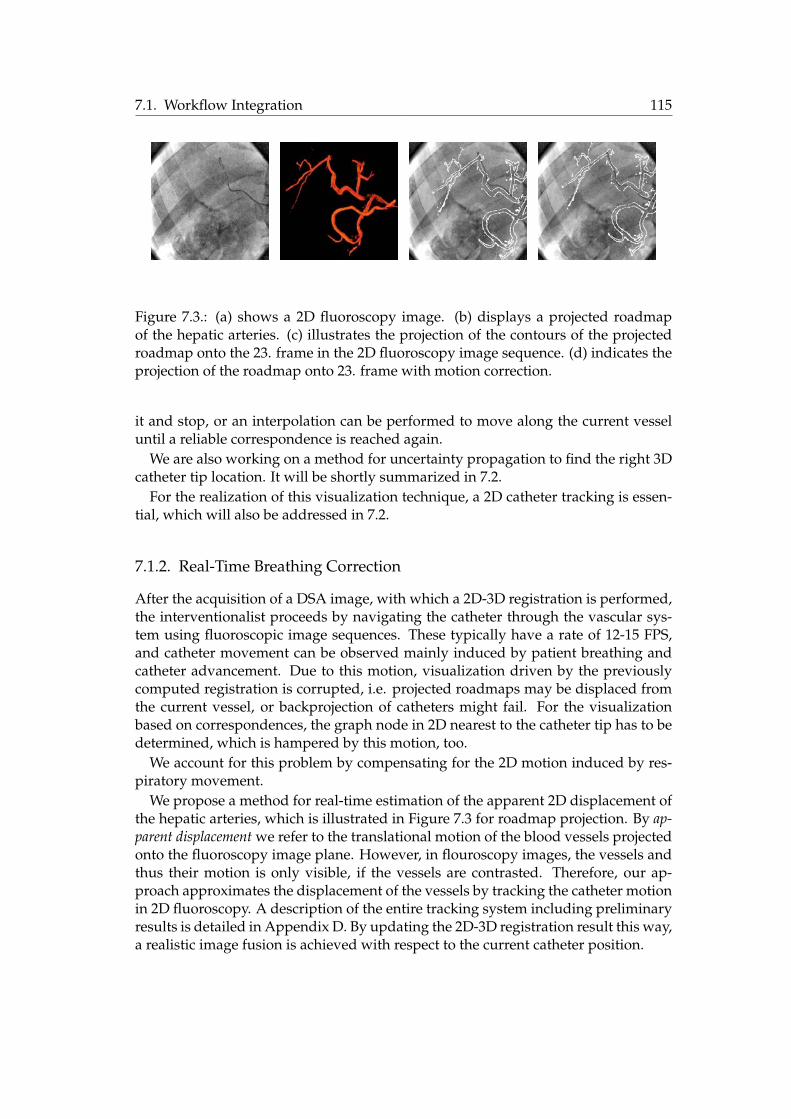
7.1. Workflow Integration 115

Figure 7.3.: (a) shows a 2D fluoroscopy image. (b) displays a projected roadmapof the hepatic arteries. (c) illustrates the projection of the contours of the projectedroadmap onto the 23. frame in the 2D fluoroscopy image sequence. (d) indicates theprojection of the roadmap onto 23. frame with motion correction.

it and stop, or an interpolation can be performed to move along the current vesseluntil a reliable correspondence is reached again.

We are also working on a method for uncertainty propagation to find the right 3Dcatheter tip location. It will be shortly summarized in 7.2.

For the realization of this visualization technique, a 2D catheter tracking is essen-tial, which will also be addressed in 7.2.

7.1.2. Real-Time Breathing Correction

After the acquisition of a DSA image, with which a 2D-3D registration is performed,the interventionalist proceeds by navigating the catheter through the vascular sys-tem using fluoroscopic image sequences. These typically have a rate of 12-15 FPS,and catheter movement can be observed mainly induced by patient breathing andcatheter advancement. Due to this motion, visualization driven by the previouslycomputed registration is corrupted, i.e. projected roadmaps may be displaced fromthe current vessel, or backprojection of catheters might fail. For the visualizationbased on correspondences, the graph node in 2D nearest to the catheter tip has to bedetermined, which is hampered by this motion, too.

We account for this problem by compensating for the 2D motion induced by res-piratory movement.

We propose a method for real-time estimation of the apparent 2D displacement ofthe hepatic arteries, which is illustrated in Figure 7.3 for roadmap projection. By ap-parent displacement we refer to the translational motion of the blood vessels projectedonto the fluoroscopy image plane. However, in flouroscopy images, the vessels andthus their motion is only visible, if the vessels are contrasted. Therefore, our ap-proach approximates the displacement of the vessels by tracking the catheter motionin 2D fluoroscopy. A description of the entire tracking system including preliminaryresults is detailed in Appendix D. By updating the 2D-3D registration result this way,a realistic image fusion is achieved with respect to the current catheter position.

116 7. Conclusion

7.2. Future Work

Catheter Detection and Tracking The correspondence-based visualization providesa tool to visualize any location in a 2D vessel simultaneously in 3D. It would be de-sirable by clinicians to have information about the catheter, in particular its tip, inthe 3D vascular tree. Thus, automatic catheter detection in 2D fluoroscopic images isimportant to fully integrate the benefits of 2D-3D registration into clinical workflow.

This detection is problematic due to the bad SNR of fluoroscopic images. More-over, bone edges that are visible in these images sometimes have the same curvilinearshape as the catheter due to its small size (about 10 pixels in a 1024 × 1024 image).These false positives make extraction algorithms prone to error. Preliminary testswith a detector of curvilinear structures proposed by Steger [137] have not broughtsatisfactory results. An interesting work that will be followed in the future is thesteerable tensor voting algorithm proposed by Franken et al. [49, 48]. A tensor fil-ter is applied to images derived from Hessian analysis to detect a catheter in noisyfluoroscopic images.

If the catheter tip has been detected in a first image, its location has to be tracked inthe following fluoroscopic frames and the tracking information has to be propagatedto 3D. We are working on an integration of results coming from registration andmotion compensation algorithms in order to predict the catheter tip location in 3Dfrom subsequent fluoroscopic frames.

Given the catheter tip location x in the last frame and a displacement d in 2Dcomputed with the apparent breathing correction method. On a sample set {yi},i = 1, . . . , n in the neighborhood of x + d we can determine the CC value CC(yi)in 2D. We get the corresponding points Yi in 3D through backprojection and closestpoint computation to the centerline points.

By randomly altering the rigid transformation parameters R, t for m times, we getnew points Zij together with energies Ej for all the new poses. For all points Yi wecan determine their covariance matrices weighted with the respective energies

Λi =1

�mj=1 E2

j

m�

j=1

Ej(Zij − Zi)�(Zij − Zi), (7.1)

where Zi is the weighted mean of Zij , j = 1, . . . , m.With these covariances, we can determine the location of the most significant sample

mode of the data as described in [33]. By incorporating the CC values CC(yi) frommotion compensation, interpreted as probabilities, into the algorithm’s weights wi,we combine uncertainties of registration and motion compensation to yield the mostprobable 3D location of the catheter. For a thorough explanation of the algorithmand preliminary results on simulated data, refer to [10].

Application and Modalities Up to now, we have applied the registration algo-rithm to data coming from the TACE procedure. On the one hand, this data showsa great variability in terms of vessel shape and deformation making it suitable foralgorithm evaluation. On the other hand, the applicability of the algorithms to other

7.2. Future Work 117

vascular images, e.g. coming from a TIPS surgery, shall be evaluated in the future.The performance of the algorithms when applied to different vessel systems willbe addressed. Moreover, the incorporation of different angiographic images will betested. Instead of preoperative CTA images, MRA data can be used, and it has to beevaluated to which extent the extractable information suffices to compute the rightregistration. Intraoperatively, it has to be evaluated if contrasted 2D fluoroscopic im-ages can also be used for the proposed methods (especially the segmentation-drivenregistration). If a detection of vessels in these images is successful despite the badSNR and the small amount of contrast agent injected, the registration can be up-dated on the fly during the procedure. This could make breathing correction as wellas catheter backprojection easier and more robust.

Tumor Visualization Integrating the tumor into the proposed visualization tech-niques is an issue that should be addressed for TACE procedures. This way, bloodvessels are shown for navigation together with the target region to be reached. Sev-eral steps have to be realized for tumor visualization and fusion with catheter andvessel locations in 3D. Since the tumor is only visible in the arterial dominant phaseof the CTA scan (see 4.4.1), it has to be registered to the angiographic phase of theCTA. This 3D-3D registration can be solved using intensity-based methods. More-over, an adequate tumor visualization has to be developed. Direct volume renderingtechniques will be rather difficult to maintain since tumor structures have a similarHounsfield unit compared to surrounding tissue, even in the arterial dominant CTAscan. Thus, a tumor segmentation from CTA would be vital to successfully illustratethe tumor region.

Intraoperative 3D Imaging Since 3D imaging is provided by C-arms nowadays,fast 3D-3D registration of vascular structures will become more important. In thisthesis, the 3D reconstruction data was used in the evaluation protocol of 2D-3D reg-istration algorithms. However, since many hospitals use intraoperative reconstruc-tions on a regular basis in vascular treatments, it should be promising to developmethods combining a 3D-3D registration with a 2D-3D refinement. The difficultyof deformation has been addressed by researches to align hepatic vessel systems forfollow-up studies [4, 29]. However, the high difference of vessel structures due tolocal and global contrast injection poses an additional difficulty that is worth beingaddressed in the future.

118 7. Conclusion

Appendix

A. Practical Considerations on Images

Computer images are rasterized, i.e. spatial locations are sampled and intensityinformation is only available at discrete points called picture or volume elements(pixel/voxel):

I : Nd0 → R (A.1)

For simplicity, we will not use the term voxel, and indicate in the text if we address2D, 3D, or ND images. We can arrange all the intensity values into a matrix (in 2D)An

m or a tensor (in 3D) Tn,mk . Often, it is necessary to retrieve the intensity value

between pixels, which can be achieved by interpolation from neighboring pixels.The neighborhood of a pixel is defined over adjacent pixels. There exist sev-

eral neighborhoods depending on dimension and integration of diagonally adja-cent pixels. For example, a 4-neighborhood in a 2D image is defined as N4(x) ={Ix−1,y+, Ix+1,y, Ix,y−1, Ix,y+1}, where we placed the locations into the subscript forbetter readability. An 8-neighborhood is defined as

N8(x) = {Ix−1,y, Ix+1,y, Ix,y−1, Ix,y+1,

Ix−1,y−1, Ix−1,y+1, Ix+1,y−1, Ix+1,y+1}.

A.1. Image Filtering

In a discrete setting convolution of two functions f, g is defined as:

(f ∗ g)(m) =�

n

f(n)g(m− n), (A.2)

Due to its frequent application (e.g. in linear scale-space), it is important to statehow the Gaussian filter is created. Usually, we create a Gaussian kernel Gσ withstandard deviation σ without evaluating the constant before ((2πσ2)N/2), but with anormalization factor

Gσ(x) = e−||x||2/2σ2

(A.3)

Gσ(x) =Gσ(x)

�x1· · ·�xn

G(A.4)

Usually we create Gσ symmetric with mean zero, so if a filter size is given by h, weevaluate the kernel at positions −(h − 1)/2 to (h − 1)/2 in each direction. The filtersize should also be adjusted to the chosen σ, a good trade-off between numericalrelevance and accuracy is h = 6 ∗ σ.

122 A. Practical Considerations on Images

A.2. Image Derivatives

On discrete images, building the derivative is a filtering process. We can derivethe image derivative from the difference quotient and image neighborhood. Thequotient should include the surroundings in a symmetrical manner and should beas local as possible. For example, for a 2D image I : N

20 → R we get:

(1) First derivative: The simplest derivative filter is the central difference operator,i.e. the mask [−1, 0, 1] filters the image in each dimension.

∂Ix,y

∂x=Ix+1,y − Ix−1,y

2h, (A.5)

where h is the element spacing between adjacent pixel. The filtering in y isanalogous.

(2) Second derivative: Here, we derive two difference quotients and build theirdifference quotient. Since we want to be symmetric and local, we take themask [−1, 1] for first derivative and [−1, 0, 1] for the second:

∂2Ix,y

∂x2= ((−1) ∗ Ix,y − Ix−1,y

h+ (Ix+1,y − Ix,y

h))/h

=Ix−1,y − 2Ix,y + Ix+1,y

h2. (A.6)

∂2Ix,y

∂y2 is analogous. Mind that due to the minimality criterion, the differencequotient is taken at x+ 1

2h and x− 12h, thus we only have to divide by h instead

of 2h for both derivation steps. The filtering in different direction is achievedby multiplying the central difference term to get a matrix filter:

[−1, 0, 1]�

�−101

��

=

�1 0 −10 0 0−1 0 1

�(A.7)

This assures symmetry again:

∂2Ix,y

∂x∂y=

Ix−1,y+1 − Ix+1,y+1 − Ix−1,y−1 + Ix+1,y−1

4h2(A.8)

Since discrete differential operators are sensitive to noise, a Gaussian smoothing isusually applied together with derivation, whose implementation is described belowtogether with linear scale-space.

A.3. Linear Scale-Space

Moving in linear scale-space is equivalent with applying a Gaussian filter with stan-dard deviation σ to an image. If we want to build first and second derivatives in

A.3. Linear Scale-Space 123

scale-space, we can, due to the commutativity of filtering and derivation, build thefilter derivative and convolve the image with the new filter:

∇Iσ = Gσ ∗ ∇I = ∇Gσ ∗ I, (A.9)

andHIσ = Gσ ∗ HI = HGσ ∗ I. (A.10)

124 A. Practical Considerations on Images

B. Thin Plate Splines

B.1. Special Spline Smoothing Problem

Given x(i) = (x1(i), . . . , xn(i))� ∈ Rn and yi ∈ R, i = 1, . . . , n, and a data model

yi = f(x1(i), · · · , xd(i)) + εi, (B.1)

where εi ∼ N(0, σ2i ) represents measurement noise.

We want to solve the special spline smoothing problem in n-dimensional Euclidean space,i.e. we want to find the minimizing function fλ to the variational problem

1n

n�

i=1

(yi − f(x1(i), · · · , xn(i)))2 + λJdm(f), (B.2)

where Jdm(f) is defined as the thin-plate penalty functional on dimension d and

derivation order m, e.g. for d = 2, m = 2

J2(f) =� ∞

−∞

� ∞

−∞(f2

x1x1+ 2f2

x1x2+ f2

x2x2)dx1dx2, (B.3)

or, for d = 3, m = 2

J2(f) =� ∞

−∞

� ∞

−∞(f2

x1x1+ f2

x2x2+ f2

x3x3+ 2[f2

x1x2+ f2

x1x3+ f2

x2x3])dx1dx2dx3. (B.4)

The solution fλ to (B.2) is given by a combination of M monomial1 coefficients andN radial function (RF) coefficients

fλ(x) =M�

ν=1

dνφν(x) +N�

i=1

ciEm(x,x(i)), (B.5)

where x = (x1, · · · , xn)�, x(i) = (x1(i), · · · , xn(i))�, and Em is Green’s functionfor the m-iterated Laplacian, (see Wahba 90 ([152]), p.30). fλ is called the Thin PlateSpline.

Informally, Em can be thought of as a radial function, i.e. a function whose re-sponse decreases (or increases) monotonically with distance from a central point (Orr96 [110]).

The resulting spline fλ has the following properties:

1A monomial is a product of positive integer powers of a fixed set of variables, for example, x, xy2, orx2y3z. In this case they are of the order < m

126 B. Thin Plate Splines

(1) Natural Spline: fλ must be a natural spline, i.e. a spline f of odd degree k =2l − 1(l ≥ 2), which satisfies

f (l+j)(a) = f (l+j)(b) = 0, j = 0, 1, · · · , l − 2 (B.6)

(2) Interpolating and Approximating Behavior: If λ = 0 we have an interpolatingbehavior, i.e. for all measured points x(i), yi : yi = fλ(x(i)), i = 0, · · · , n. Ifλ = 0 we have an approximating behavior, i.e. for all measured points x(i), yi :yi ≈ fλ(x(i)), i = 0, · · · , n, such that the SSD is minimized:

minf

(yi − f(x(i)))2 (B.7)

(3) Existence of Squared Integral: In order to fulfill the smoothness condition, thesquared integral must exist, i.e.

� ∞

−∞(f (m)(t))2dt < ∞ (B.8)

(4) Smoothness Condition: The thin-plate penalty functional Jdm(f), the integral of

squared derivatives of order m, must be minimized. Thus, the resulting splineis smooth (has low curvature).

B.2. Numerical Solution

We want to find the coefficients dν , ci of fλ. For that, we rewrite the equation as asystem of linear equations in matrix-vector form. For each measurement yi ↔ x(i)we write the constraints

yi =M�

ν=1

dνφν(x(i)) +N�

j=1

cjEm(x(i),x(j)), (B.9)

in matrix-vector form

Kc + Pd = y (B.10)P�c = 0, (B.11)

where K ∈ RN×N , Kij = Em(x(i),x(j)) only consists of the radial functions evalu-

ated at all measured x-vectors x(i) (independent of yi).P ∈ R

N×M , Pij = φj(x(i)) accounts for the coefficients of the monomial partwith all measured points x(i), and y = (y1, · · · , yn) are all measurements in the co-domain.

Equation (B.10) accounts for the constraints given by the function fλ. Equation(B.11) accounts for the square integrability of fλ, and simply forces the derivative ofthe elastic part of fλ, ciEm(x,x(i))(m), to be 0 at infinity.

B.3. TPS for Feature-Based Deformable Registration 127

In the upper equations we require an interpolation behavior, i.e. f(x(i)) = yi.However, we have noisy measurement data and want to have an approximationbehavior, i.e. f(x(i)) ≈ yi, such that the sum of squared differences in equation (B.2)is minimized. This can be achieved by introduction of the regularization parameterλ into the numerical solution:

�K + nλW−1

�c + Pd = y (B.12)

P�c = 0, (B.13)

where W−1 = diag(σ21, . . . , σ

2n) is the matrix of variances of the noise distribution of

the measurements, or W−1 = I if unknown.Altogether, we have to solve for the vector [c d]� in the system of linear equations

�������������

y1

y2...

yn

0...0

�������������

=

K + nλW−1 PP� 0

·

cd

, (B.14)

which can be accomplished using standard numerical solvers, e.g. the Singular ValueDecomposition (SVD).

B.3. TPS for Feature-Based Deformable Registration

The TPS is particularly suitable for the task of feature-based deformable registra-tion as introduced by Bookstein [15] for medical image registration and extensivelystudied by Rohr [126].

Given m points Xi = (xi1, . . . , xin)� ∈ FA and Yi = (yi1, . . . , yin)� ∈ FB repre-senting corresponding point features extracted from images A,B.

We want to find a transformation ϕ that minimizes the squared distance of all cor-responding points. Moreover, we want the transformation to be sufficiently smooth,i.e. no folding or tearing should be introduced. Mathematically, we want to find ϕ,such that

E =n�

i=1

||Xi − ϕ(Yi)||2 + λJ2(ϕ) (B.15)

is minimal. J2 is called the thin-plate penalty functional (see Equations (B.3) and(B.4)) and penalizes the curvature of the transformation ϕ in order to keep it smooth.

The TPS is given by ϕ′ = (ϕ′1, . . . , ϕ′n)�, where ϕ′l models an affine transformationpart (n + 1 monomials), and a local deformation part (m radial functions):

ϕ′l(X) = a0 +n�

j=1

ajxj +m�

k=1

wkU(|Xk −X|), (B.16)

128 B. Thin Plate Splines

where a0, . . . , an are the parameters controlling the affine part and w1, . . . , wm arethe parameters controlling the local non-rigid part. These n(n + 1) affine and nmnon-rigid parameters are determined from the point correspondences {Xi ↔ Yi}.U(.) is a radial function and defined as U(r) = r2ln(r) in 2D and as U(r) = |r| in 3D[146].

TPS registration has advantages and drawbacks. First, it can be computed on ar-bitrary points in space and retrieve a function with global support, i.e. the controlpoints do not have to be uniformly distributed as for functions with local support,e.g., cubic B-splines [63]. Moreover, it is no mere interpolation scheme, but can beused as an approximation scheme, minimizing Equation (B.15) for all points in theimage domains. Doing that, it also penalizes for high variations in curvature of thedisplacement field making sure that it transforms “sufficiently smooth”. And last,but not least, TPS are very easy to implement and, for a smaller number of controlpoints, computationally efficient.

However, TPS-based registration is rather restricted. It cannot minimize otherdistance measures than mono-dimensional Euclidean, or Mahalanobis distance andthus always has to operate on point sets. Due to this rigidity of the formulation,it cannot be extended to 2D-3D deformable registration. Furthermore, it minimizesone particular smoothing term and cannot be extended to other, maybe more con-venient smoothing terms without loosing the theoretical minimizing property. Thefeature point correspondences (control points) have infinite support, i.e. all controlpoints contribute to the deformation of other points. Thus, it is rather difficult topredict or change local behavior using TPS.

As mentioned in section 2.3.2, a local transformation should fulfill the propertiesof a diffeomorphism. Unfortunately, a TPS is no diffeomorphic mapping, but it canbe extended to one as shown by Camion and Younes [24] in the form of geodesicinterpolating splines. They have been successfully applied to Medical Image Analysisby Twining and Marsland [146].

C. Rotation Parameterization

C.1. Euler Angles

A minimal (and maybe the most intuitive) parameterization of a rotation matrix isgiven by three Euler angles, α, β, γ, representing the 3 DOF. These angles representthe rotations around the cartesian coordinate axes in 3D, i.e. x-, y-, and z-axis. Theorder of rotation is important to keep consistent, we choose the ZY X1 order, i.e.first rotate around x-axis (Rx(α)), then around y-axis (Ry(β)), finally around z-axis(Rz(γ)):

X′ = Rz(γ)Ry(β)Rx(α)X, (C.1)

where the respective rotation matrices are given by

Rx(α) =

���

1 0 00 cos α − sin α0 sin α cos α

��� , Ry(β) =

���

cos β 0 sinβ0 1 0

− sin β 0 cos β

��� ,

Rz(γ) =

���

cos γ − sin γ 0sin γ cos γ 0

0 0 1

��� ,

the mutliplication of them gives the rotation matrix

R =

���

cβ cα −cγ sα + sγ sβ cα sγ sα + cγ sβ cαcβ sα cγ cα + sγ sβ sα −sγ cα + cγ sβ sα−sβ sγ cβ cγ cβ

��� , (C.2)

where cα = cos α, sα = sinα, etc.With this equation we can calculate a rotation matrix given three angles and vice

versa.

C.2. Gimbal Lock

A singularity exists, known as Gimbal Lock, which is the ambiguity to determineangles α, γ if β = ±Π/2. In this case, the rotation matrix looks like

R(β = π/2) =

���

0 −cγ sα + sγ cα sγ sα + cγ cα0 cγ cα + sγ sα −sγ cα + cγ sα−1 0 0

��� . (C.3)

1read from right to left, since we do left-sided matrix multiplications

130 C. Rotation Parameterization

Using simple trigonometry, we get

R(β = π/2) =

���

0 sin (γ − α) cos (γ − α)0 cos (γ − α) − sin (γ − α)−1 0 0

��� , (C.4)

which is a rotation with angle δ = γ − α. Since there are many combinations to getthe same δ from γ and α, there is an ambiguity, which has to be considered whenconverting rotation matrices to α, β, γ. For β = −Π/2 there is an analogous calcula-tion. As convention, in both cases (β = ±Π/2) we choose α = 0, thus resolving forthis ambiguity.

C.3. Euler Angles in Rigid Registration

For the task of rigid registration, we usually alter the Euler angles and form a rota-tion matrix to transform an image or point. That is, the Euler representation of therotation is changed during the (non gradient-based) optimization process, the rota-tion matrix just has to be built from the new parameters for energy term evaluation.In this direction, no ambiguity arises. Since we are never converting a rotation ma-trix to Euler angles in the registration process, only for visualization purposes, ourresults are not flawed by the Gimbal Lock.

If we use a gradient-based optimizer, the parameterization has to be used forbuilding the first (and maybe second) derivative of the energy term. In this case,the ambiguity of Euler Angles is important and another parameterization of a rota-tion matrix should be used. Since all our rigid registration algorithms use a directoptimizer, which is not using the gradient of the energy term, we preferred the intu-itive representation of rotations to a rotation reparameterization.

There are other representations of rotations, e.g. unit quaternions, or axis-anglerepresentation (via the Rodriguez formula). However, these representations havefour parameters and are constrained by vector unit length, while the minimal num-ber of parameters for a rotation is three. Thus, if we run a parameter optimization,the parameter space increases by one, which might influence convergence rate andnumerical stability of the registration.

Since we do not have to suffer from the Gimbal Lock (as the Computer Graphicscommunity does) and since Euler Angles are minimal in terms of rotation param-eterization, we use them throughout the thesis and discard other possible rotationparameterizations.

D. Real-Time Respiratory Motion Tracking

We propose a method for real-time estimation of the apparent 2D displacement of thehepatic arteries, which is illustrated in Figure 7.3 for roadmap projection. By apparentdisplacement we refer to the translational motion of the blood vessels projected ontothe fluoroscopy image plane. However, in flouroscopy images, the vessels and thustheir motion is only visible, if the vessels are contrasted. Therefore, our approachapproximates the apparent displacement of the vessels by tracking the catheter mo-tion in 2D fluoroscopy. By updating the 2D-3D registration result this way, a realisticimage fusion is achieved with respect to the current catheter position.

In the following, we will summarize the proposed method and show some prelim-inary results. A extensive study and more details on the numerical implementationto fulfill the real-time constraint are given in [3].

D.1. Method

D.1.1. Motion Model

Clifford et al. [32] present an extensive assessment of respiratory hepatic motionbased on nine previously published studies. All studies agree that the most signif-icant component of liver motion is cranio-caudal translation. There exists disagree-ment in the literature about the significance of liver motion in anterior-posterior andlateral directions. Recent studies, which follow the motion of single or multiplepoints within the liver volume, indicate that respiration causes significant transla-tional motion along both of these axes, whereas earlier studies, which evaluate themotion of liver margins, suggest that clinically significant liver motion can be ap-proximated effectively by cranio-caudal translation alone [32]. The tissue deforma-tion caused by respiration is reported to be 3 mm on average. Rohlfing et al. [124, 125]estimate an average tissue deformation of 6-10 mm by comparison of rigid and non-rigid registration of the liver. However, they report that the rigid motion model i.e.translation and rotation accurately aligned the central area, while residual deforma-tion occurs mostly in the periphery [32]. The same group reports that the rotationsdid not exceed 1.5 degrees. Considering these studies we approximate the apparentdisplacement of vessels due to respiration in 2D fluoroscopy images using a globaltranslational model that covers translations in both x- and y-directions in the imageplane. Our method does not account for local vessel deformations currently.

D.1.2. Approximation of Vessel Motion by Catheter Motion

As non-contrasted hepatic arteries are not visible in 2D fluoroscopy images, our ap-proach approximates their apparent 2D respiratory displacement from catheter mo-

132 D. Real-Time Respiratory Motion Tracking

tion. Since the catheter is located within the vessels, its motion inevitably comprisesthe vessel motion. However, the catheter motion is further complicated by defor-mations. Because of the branched and elastic nature of the vessels a considerabledeformation of the catheter occurs while being advanced by the interventional radi-ologist. For the robustness of the algorithm against these catheter deformations wepropose an appropriate dynamic template update strategy.

D.1.3. Motion Tracking on Enhanced Images

Fluoroscopic images have a high SNR due to the low radiation dose used for acquisi-tion. In order to enhance the catheter and suppress noise, a filtering is applied to theoriginal fluoroscopy images. Regarding the width of a catheter, we apply a modifiedMarr-Hildreth filter, as proposed by Palti-Wasserman et al. [114].

After the filtering step the apparent 2D displacement of the catheter is estimatedby template matching. Thereby, the displacement d = (dx, dy) of a structure betweentwo frames is computed by defining a template T in one frame containing this struc-ture and by finding the region which matches it in the other frame I with respect toa chosen similarity measure. Because of its robustness against noise and linear illu-mination changes we use the Correlation Coefficient (CC) as a similarity measure.For estimating the global translational motion we only consider a small part of thecatheter, which has to contain both a vertical and a horizontal component in orderto avoid the well-known aperture problem. In the initialization step of the trackingalgorithm we ask the interventional radiologist to draw a small rectangle in the firstframe covering such a part of the catheter. Then, a template matching is performedin a search region bigger than the largest expected translation induced by respira-tory motion (up to 9mm in x- and 45 mm in y-direction, refer to Clifford et al. [32]).For tracking the motion between consecutive frames the search region is translatedwith the last computed displacement for each frame and the template matching is in-voked in a smaller search region (up to 17 mm in x- and 25 mm in y-direction provedto be sufficient in our experiments). With this technique, the search region is keptsmall, which provides an acceleration in runtime of the algorithm and also decreasesthe probability of matching the catheter with other line-like structures such as bones.Moreover, the large influence of the catheter within the small template assures a re-liable response of the CC for estimating the motion induced by breathing.

D.1.4. Dynamic Template Update

Using the same template for the entire intervention involves the assumption that theappearance of the catheter part contained in the template does not change over time.As the appearance of the catheter changes due to its deformation induced by theradiologist’s movement, the algorithm will fail in general using only the templatecreated from the first frame. In order to deal with possible catheter deformations weupdate the template if there is a considerable change in the structure contained in thetemplate. We perform the template update if the difference between best CC values

D.2. Results 133

of the initial and current frame becomes too large. As the new template we use theregion that yields the maximum score of CC in the previous frame.

D.2. Results

The accuracy of the algorithm and its robustness against noise and catheter defor-mation is tested using both simulated and clinical image sequences.

D.2.1. Simulation Studies

In order to perform a quantitative analysis with a known ground truth, we generateimage sequences by artificially superimposing a catheter onto real 2D fluoroscopysequences of 15 frames. In these images, the catheter is manually removed and thecorresponding region is inpainted by bilinear interpolation. By using clinical imagesand real catheter intensities, we assure that the simulated images are realistic (Fig.D.2.1). The position of the catheter is changed over the frames by a translation in ydirection, which is to be corrected with our method. Starting with zero displacement,over the first 7 frames, the total displacement is increased by 4.8 mm between singleframes, and in the second 7 frames, it is decreased by the same amount, resulting ina rough approximation of the respiratory motion visible in the images. This resultsin a maximal displacement of 33.6 mm. Using this setting, we perform two tests: onein which the added catheter is deformed, and a second, in which the robustness tonoise is tested.

The accuracy of the algorithm in presence of catheter deformation is tested on thedescribed sequence in 12 tests with different magnitudes of deformation (1.2-14.6mm), resulting in a total of 180 simulated frames. To this end, the artificial catheteris deformed, before adding it to the background sequence. The deformation is per-formed by randomly moving 100 points of a free-form deformation (FFD) modelbased on cubic B-splines.

For all magnitudes of catheter deformation, the mean error of the computed dis-placements remains small (0.26-1.21mm).

The influence of noise is tested by adding different amounts of Gaussian noise tothe sequence presented above in 10 tests, resulting in 150 simulated image frames.In this test, no deformation is added to the catheter. Note that the simulated imagesalso contain the regular amount of signal dependent Poisson noise present in the X-ray beams, since they are created by manipulating clinical image sequences. By anadditional Gaussian noise with variance of between 0.1% and 5% of the maximumimage intensity (Fig. D.2.1) the mean error of the algorithm is between 0.00 mm and0.89 mm.

D.2.2. Patient Studies

In order to evaluate the accuracy of the algorithm on real data we segment thecatheter in 164 frames of a clinical image sequence and measure the fraction of catheter

134 D. Real-Time Respiratory Motion Tracking

Figure D.1.: (a) shows a frame from a simulated image sequence with known catheterdisplacements. (b) displays the effect of additional Gaussian noise in the simulatedimage sequence, whereas the rectangular region is used as template by motion track-ing. (c) and (d) illustrate the average and standard deviation of the error in patientdata study with respect to template size.

contained in the vessel by computing |NC ∩ NR|/|NC |, with NC and NR being thesegmented pixels of the catheter and the roadmap respectively. Our motion correc-tion improves the catheter overlap from 36% to 70%. The influence of template sizeand location on the success of the algorithm is studied on 4 clinical fluoroscopy im-age sequences (with a total of 571 frames). For that, three inexperienced users selectthree points on the catheter for each sequence. Centered at each point 38 templateswith different sizes between 3×3 pixels and 150×150 pixels are created. During thetests the size of the search region is set to the size of the template plus an extension inx and y direction of 20 and 40 pixels, respectively. The algorithm is then performedusing each template. In the absence of an absolute ground truth, we compare the

D.2. Results 135

results to the displacements determined by manually defined motion correction. Foreach user the average and standard deviation of the mean error over all frames isdisplayed in Fig. D.2.1 and D.2.1 respectively. The error in one frame is computed as‖de − (dp1 + dp2 + dp3)/3‖, where de denotes the expected displacement and dp1 ,dp2 , dp3 denote the computed displacements using template centered at points p1,p2 and p3, respectively. For all templates of size between 20 × 20 and 80 × 80 theerror of the algorithm is in average 1.25 mm with a standard deviation less than 0.44mm. Such an error is visually barely noticeable. and admissible for hepatic arterycatheterizations. This study shows that the method still leads to near-optimal resultsfor a large range of template sizes and for different template locations. Thus, we canconclude that the method does not require a precise template creation but involvesjust a simple user interaction, which is admissible for hepatic artery catheterizationsas confirmed by our clinical partners.

136 D. Real-Time Respiratory Motion Tracking

E. List of Symbols

Energies

E the energy term

D the data term

S the regularization term

Graphs

Gd a graph with node set V d and edge set Ed, where d represents the spatialdimension of nodes in V d. The graph consists of bifurcation points B ∈V d

b and sampling points X ∈ V ds . V d = V d

b ∪ V ds , V d

b ∩ V ds = ∅. Sampling

nodes always have two neighbors, i.e. their degree is 2.

Πi,j a segment between two bifurcation nodes Bi,Bj , only consisting ofsampling nodes and edges between them.

Gt a topological graph, only consisting of bifurcation nodes and edges be-tween them, i.e. Gt = (V d

b , Et), where Et ⊂ V db × V d

b .

Images

I an image, i.e. an intensity mapping from a spatial domain to a real num-ber Ω → R

∇I the gradient of image IHI the Hessian matrix (second derivative) of image I

138 E. List of Symbols

Projections

P a projection matrix, i.e. a mapping from P3 to P

2

K the calibration matrix of a pinhole camera

R a rotation matrix

t a translation vector

fP a projection function, i.e. a mapping from R3 to R

2 defined by the pro-jection matrix P

Statistics

X a (multivariate) random variable

X a value of a (multivariate) random variable X

P (X ) the probability of random variable X having the value X (abbreviationto P (X = X )

P (X|Y) the probability of random variable X having the value X given thatvariable Y has the value Y (abbreviation to P (X = X|Y = Y)

G(μ, σ) Gaussian distribution with mean μ and standard deviation σ

Gσ(X ) Gaussian distribution with zero mean and standard deviation σ evalu-ated at X .

Transformations

ϕ a transformation, which is usually a vector-valued function

∇ϕ the first derivative of ϕ

Jϕ the Jacobian matrix of ϕ. This is equal to the first derivative of ϕ, i.e.Jϕ = ∇ϕ.

ϕi the transformation at a particular point xi

Θ a transformation parameter

139

Vectors and Matrices

x some 2D vector, i.e. x = (x, y)�

X some 3D vector, i.e. X = (x, y, z)�

x a homogeneous 2D vector, i.e. x = (x, y, w)� ∈ P2

X a homogeneous 3D vector, i.e. X = (x, y, z, w)� ∈ P3

M a matrix

140 E. List of Symbols

F. List of Abbreviations

Medical Terms

HCC Hepatocellular Carcinoma

ROI Region of Interest

TACE Transarterial Chemoembolization

TIPS Transjugular Intrahepatic Portosystemic Shunt

Medical Imaging Modalities

CT Computed Tomography

CTA Computed Tomography Angiography

DSA Digitally Subtracted Angiography

HU Hounsfield Unit

MR Magnetic Resonance (Imaging/Tomography)

MRA Magnetic Resonance (Imaging/Tomography) Angiography

MRA TOF MRA Time of Flight

MRA PC MRA Phase Contrast

US Ultrasound

Similarity Measures

142 F. List of Abbreviations

CC Correlation Coefficient

ECC Entropy Correlation Coefficient

GD Gradient Difference

GC Gradient Correlation

MI Mutual Information

NCC Normalized Cross Correlation

PI Pattern Intensity

SM Similarity Measure

SSD Sum of Square Differences

(Numerical) Algorithms

ART Algebraic Reconstruction Technique

FBP Filtered Back Projection

HSA Hybrid Simulated Annealing

ICP Iterative Closest Point

IIP Iterative Inverse Perspective

LAP Linear Assignment Problem

SVD Singular Value Decomposition

Deformations

FFD Free Form Deformation

TPS Thin Plate Spline

Projections

CCS Camera Coordinate System

DRR Digitally Reconstructed Radiograph

MIP Maximum Intensity Projection

WCS World Coordinate System

143

Errors

PD projection distance

RMSE Root Mean Square Error

RPD reprojection distance

TRE target registration error

Miscellaneous

FPS frames per second

GPU Graphics Processing Unit

SNR signal-to-noise ratio

144 F. List of Abbreviations

G. List of Publications

International Journals

GROHER, M., JAKOBS, T.F., PADOY, N., AND NAVAB, N. Planning and Intraopera-tive Visualization of Liver Catheterizations: New CTA Protocol and 2D-3D Registra-tion Method. Academic Radiology 14 (11), pp. 1324–1339, 2007.

NAVAB, N., AND GROHER, M. Novel Navigation and Advanced Visualization Tech-niques for Abdominal Catheterization. Hospital Imaging and Radiology Europe 2 (4),pp.29-30, 2008.

GROHER, M., ZIKIC, D., AND NAVAB, N. Deformable Registration of 3D VesselStructures to a Single Projection Image. Submitted to IEEE Transactions on MedicalImaging.

International Conferences

UNGER, C., GROHER, M., AND NAVAB, N. Image Based Rendering for Motion Com-pensation in Angiographic Roadmapping. IEEE Computer Society Conference on Com-puter Vision and Pattern Recognition (CVPR), Anchorage, USA, 2008.

ZIKIC, D., GROHER, M., KHAMENE, A., AND NAVAB, N. Deformable Registrationof 3D Vessel Structures to a Single Projection Image. SPIE Medical Imaging, San Diego,USA, 2008.

ATASOY, S., GROHER, M., ZIKIC, D., GLOCKER, B., WAGGERSHAUSER, T., PFISTER,M., AND NAVAB, N. Real-Time Respiratory Motion Tracking: Roadmap Correctionfor Hepatic Artery Catheterizations. SPIE Medical Imaging, San Diego, USA, 2008.

GROHER, M., BENDER, F., HOFFMANN, R.T., AND NAVAB, N. Segmentation-Driven2D-3D Registration for Abdominal Catheter Interventions. Medical Image Computingand Computer-Assisted Intervention (MICCAI) (2007), pp. 527-535.

GROHER, M., PADOY, N., JAKOBS, T.F., AND NAVAB, N. New CTA Protocol and2D-3D Registration Method for Liver Catheterization. In Medical Image Computingand Computer-Assisted Intervention (MICCAI) (2006), pp. 873–881.

146 G. List of Publications

National Conferences

GROHER, M., HOFFMANN, R.T, ZECH, C.J., REISER, M., NAVAB, N. An EfficientRegistration Algorithm for Advanced Fusion of 2D/3D Angiographic Data. In Bild-verarbeitung fuer die Medizin (BVM) (2007).

KOENIG, L., GROHER, M., KEIL, A., GLASER, CH., REISER, M., NAVAB, N. Semi-Automatic Segmentation of the Patellar Cartilage in MRI. In Bildverarbeitung fuer dieMedizin (BVM) (2007).

GROHER, M., JAKOBS, T.F., REISER, M., NAVAB, N. Advanced 2D-3D Registra-tion Method for Transarterial Chemoembolizations. 5. Jahrestagung der DeutschenGesellschaft fur Computer-und Roboter-Assistierte Chirurgie (CURAC) (2006).

GROHER, M., JAKOBS, T.F., PADOY, N., NAVAB, N. Towards a Feature-based 2D-3DRegistration Method of CTA and 2D Angiograms for Liver Tumor Chemoembolizations.4. Jahrestagung der Deutschen Gesellschaft fur Computer-und Roboter-Assistierte Chirurgie(CURAC) (2005).

BAUERNSCHMITT, R., SCHIRMBECK, E.U., GROHER, M., KEITLER, P., BAUER, M.,NAJAFI, H., KLINKER, G., LANGE, R. Navigierte Platzierung endovaskularer Aorten-stents. Z Kardiologie 93 S3: 116 (2004).

Bibliography

[1] ALPERIN, N., LEVIN, D. N., AND PELIZZARI, C. A. Retrospective registrationof X-ray angiograms with MR images by using vessels as intrinsic landmarks.Journal of Magnetic Resonance Imaging (JMRI) 4 (1994), 139–144.

[2] ALT, H., AND GODAU, M. Computing the Frechet distance between twopolygonal curves. International Journal of Computational Geometry and Appli-cations (IJCGA) 5 (1995), 75–91.

[3] ATASOY, S. Real-time respiratory motion tracking: Roadmap correction forendovascular interventions. Master’s thesis, Technische Universitat Munchen,2007.

[4] AYLWARD, S., AND JOMIER, J. Rigid and deformable vasculature-to-imageregistration: A hierarchical approach. In Proc. Int’l Conf. Medical Image Com-puting and Computer Assisted Intervention (MICCAI) (2004), vol. 3216 of LectureNotes in Computer Science, Springer, pp. 829–836.

[5] AYLWARD, S., JOMIER, J., WEEKS, S., AND BULLITT, E. Registration and anal-ysis of vascular images. Int’l Journal of Computer Vision (IJCV) 55 (2003), 123–138.

[6] AYLWARD, S. R., AND BULLITT, E. Initialization, noise, singularities, and scalein height ridge traversal for tubular object centerline extraction. IEEE Trans. onMedical Imaging (TMI) 21, 2 (2002), 61–75.

[7] BANSAL, R., STAIB, L. H., CHEN, Z., RANGARAJAN, A., KNISELY, J., NATH,R., AND DUNCAN, J. S. Entropy-based, multiple -portal-to-3DCT registrationfor prostate radiotherapy using iteratively estimated segmentation. In Proc.Int’l Conf. Medical Image Computing and Computer Assisted Intervention (MICCAI)(1999), Lecture Notes in Computer Science, Springer, pp. 567–578.

[8] BELONGIE, S., MALIK, J., AND PUZICHA, J. Shape matching and object recog-nition using shape contexts. IEEE Trans. Pattern Anal. Mach. Intell. (PAMI) 24(2002), 509–522.

[9] BENAMEUR, S., MIGNOTTE, M., PARENT, S., LABELLE, H., SKALLI, W., AND

DE GUISE, J. 3D/2D registration and segmentation of scoliotic vertebra usingstatistical models. Computerized Medical Imaging and Graphics 27 (2003), 321–337.

[10] BENDER, F. Segmentation, 2D-3D registration, and uncertainty propagationfor dynamic roadmapping in angiographic interventions. Master’s thesis,Technische Universitat Munchen, 2007.

148 Bibliography

[11] BESL, P. J., AND MCKAY, D. A method for registration of 3-D shapes. IEEETrans. Pattern Anal. Mach. Intell. (PAMI) 14 (1992), 239–256.

[12] BIRKFELLNER, W., SEEMANN, R., FIGL, M., HUMMEL, J., EDE, C., HO-MOLKA, P., YANG, X., NIEDERER, P., AND BERGMANN, H. Fast DRR gen-eration for 2D/3D registration. In Proc. Int’l Conf. Medical Image Computing andComputer Assisted Intervention (MICCAI) (2005), pp. 960–967.

[13] BITTER, I., KAUFMAN, A., AND SATO, M. Penalized-distance volumetricskeleton algorithm. IEEE Trans. on Visualization and Computer Graphics 7, 3(July-Sept. 2001), 195–206.

[14] BLUM, H., AND NAGEL, R. N. Shape description using weighted symmetricaxis features. Pattern Recognition 10, 3 (1978), 167–180.

[15] BOOKSTEIN, F. L. Principal warps: Thin-plate splines and decomposition ofdeformations. IEEE Trans. Pattern Anal. Mach. Intell. (PAMI) 11 (1989), 567–585.

[16] BORGEFORS, G. Distance transformations in digital images. Comput. Vis.,Graph., Image Processing 34 (1986), 344–371.

[17] BOUIX, S., SIDDIQI, K., AND TANNENBAUM, A. Flux driven automatic cen-terline extraction. Medical Image Analysis 9 (2005), 209–221.

[18] BRONSTEIN, I. N., SEMENDJAEV, K. A., MUSIOL, G., AND MUHLIG, H.Taschenbuch der Mathematik, 5 ed. Deutsch, 2000.

[19] BROWN, L. G. A survey of image registration techniques. ACM Comput. Surv.24, 4 (1992), 325–376.

[20] BROX, T., ROSENHAHN, B., AND WEICKERT, J. Three-dimensional shapeknowledge for joint image segmentation and pose estimation. In Pattern recog-nition : 27th DAGM Symposium (2005), Lecture Notes in Computer Science,Springer, pp. 109–116.

[21] BULLITT, E., LIU, A., AYLWARD, S., COFFEY, C., STONE, J., MUKHERJI, S.,AND PIZER, S. Registration of 3D cerebral vessels with 2D digital angiograms:Clinical evaluation. Academic Radiology 6 (1999), 539–546.

[22] BURT, P. Fast filter transforms for image processing. Computer Vision, Graphics,and Image Processing 16 (1981), 20–51.

[23] BYRNE, V., COLOMINAS, C., HIPWELL, J., COX, T., NOBLE, J., PENNEY, G.,AND HAWKES, D. Assessment of a technique for 2D-3D registration of cerebralintra-arterial angiography. British Journal of Radiology 77 (2004), 123–128.

[24] CAMION, V., AND YOUNES, L. Geodesic interpolating splines. In Proc. ofthe 3rd Int’l Workshop on Energy Minimization Methods in Computer Vision andPattern Recognition (EMMCVPR) (London, UK, 2001), Springer, pp. 513–527.

Bibliography 149

[25] CAN, A., SHEN, H., TURNER, J., TANENBAUM, H., AND RAYSAM, B. Rapidautomated tracing and feature extraction from retinal fundusimages usingdirect exploratory algorithms. IEEE Transactions on Information Technology inBiomedicine 3, 2 (1999), 125–138.

[26] CASELLES, V., KIMMEL, R., AND SAPIRO, G. Geodesic active contours. Int’lJournal of Computer Vision (IJCV) 22, 1 (1997), 61–79.

[27] CHAN, H., CHUNG, A., YU, S., AND WELLS, W. 2D-3D vascular registra-tion between digital subtraction angiographic (DSA) and magnetic resonanceangiographic (MRA) images. In Proc. of the IEEE International Symposium onBiomedical Imaging (2004), vol. 1205 of Lecture Notes in Computer Science, IEEE,pp. 708–711.

[28] CHAN, T., AND VESE, L. Active contours without edges. IEEE Trans. on ImageProcessing 10, 2 (Feb. 2001), 266–277.

[29] CHARNOZ, A., AGNUS, V., MALANDAIN, G., NICOLAU, S., TAJINE, M., AND

SOLER, L. Design of robust vascular tree matching: validation on liver. In Proc.Int’l Conf. Information Processing in Medical Imaging (IPMI) (2005), vol. 3565 ofLecture Notes in Computer Science, Springer, pp. 443–455.

[30] CHOI, Y., AND LEE, S. Injectivity conditions of 2D and 3D uniform cubic B-Spline functions. Graphical Models 62, 6 (2000), 411–427.

[31] CHUI, H., AND RANGARAJAN, A. A new point matching algorithm for non-rigid registration. Computer Vision and Image Understanding 89 (2003), 114–141.

[32] CLIFFORD, M., BANOVAC, F., LEVY, E., AND CLEARY, K. Assessment of hep-atic motion secondary to respiration for computer assisted interventions. Com-puter Aided Surgery 7, 5 (2002), 291–299.

[33] COMANICIU, D. Nonparametric information fusion for motion estimation. InProc. Conf. Computer Vision and Pattern Recognition (CVPR) (2003), pp. 59–66.

[34] CONDURACHE, A., AND AACH, T. Vessel segmentation in angiograms usinghysteresis thresholding. In 9th IAPR Conference on Machine Vision Applications(MVA2005) (Tsukuba, May 16–18 2005), IAPR (ISBN: 4-901122-04-5), pp. 269–272.

[35] CONDURACHE, A., AACH, T., GRZYBOWSKI, S., AND MACHENS, H.-G. Ves-sel segmentation and analysis in laboratory skin transplant micro-angiograms.In Proc. 8th IEEE Symposium on Computer-Based Medical Systems (CBMS) (23-24June 2005), pp. 21–26.

[36] CROWLEY, J. L. A Representation for Visual Information. PhD thesis, CarnegieMellon University, 1981.

150 Bibliography

[37] DEMPSTER, A. P., LAIRD, N. M., AND RUBIN, D. B. Maximum likelihoodfrom incomplete data via the EM algorithm. Journal of the Royal Statistical Soci-ety. Series B (Methodological) 39, 1 (1977), 1–38.

[38] DESCHAMPS, T., AND COHEN, L. Fast surface and tree structure extractionof vascular objects in 3D medical images. In Fifth International Conference onCurves and Surfaces (Saint-Malo, France, June 2002), pp. 103–112.

[39] DEY, J., AND NAPEL, S. Targeted 2D/3D registration using ray normalizationand a hybrid optimizer. Medical Physics 33, 12 (2006), 4730–4738.

[40] EBERLY, D. Ridges in Data and Image Analysis. Kluwer, 1996.

[41] FELDMAR, J., AYACHE, N., AND BETTING, F. 3D-2D projective registrationof free-form curves and surfaces. In Proc. Int’l Conf. of Computer Vision (ICCV)(1995), vol. 20-23, IEEE, pp. 549–556.

[42] FISCHER, B., AND MODERSITZKI, J. Curvature based image registration. Jour-nal of Mathematical Imaging and Vision 18, 1 (2003), 81–85.

[43] FISHMAN, E. K. Cardiac CT: Where are we today and where are we going?Applied Radiology Online (Supplement) 35 (2006), 5–9.

[44] FISHMAN, E. K., AND LAWLER, L. P. CT angiography: Principles, tech-niques and study optimization using 16-slice multidetector CT with isotropicdatasets and 3D volume visualization. Critical Reviews in Computed Tomography45 (2004), 355–388.

[45] FLEUTE, M., AND LAVALLEE, S. Nonrigid 3-D/2-D registration of images us-ing statistical models. In Proc. Int’l Conf. Medical Image Computing and ComputerAssisted Intervention (MICCAI) (London, UK, 1999), Springer, pp. 138–147.

[46] FRANGI, A., NIESSEN, W., HOOGEVEEN, R., VAN WALSUM, T., AND

VIERGEVER, M. Model-based quantitation of 3-D magnetic resonance angio-graphic images. IEEE Trans. on Medical Imaging (TMI) 18, 10 (Oct. 1999), 946–956.

[47] FRANGI, A. F., NIESSEN, W. J., VINCKEN, K. L., AND VIERGEVER, M. A.Multiscale vessel enhancement filtering. In Proc. Int’l Conf. Medical Image Com-puting and Computer Assisted Intervention (MICCAI) (1998), vol. 1496 of LectureNotes in Computer Science, Springer, pp. 130–137k.

[48] FRANKEN, E., RONGEN, P., VAN ALMSICK, M., AND TER HAAR ROMENY,B. M. Detection of electrophysiology catheters in noisy fluoroscopy images.In Proc. Int’l Conf. Medical Image Computing and Computer Assisted Interven-tion (MICCAI) (2006), vol. 4191 of Lecture Notes in Computer Science, Springer,pp. 25–32.

Bibliography 151

[49] FRANKEN, E., VAN ALMSICK, M., RONGEN, P., FLORACK, L., AND TER

HAAR ROMENY, B. M. An efficient method for tensor voting using steerablefilters. In Eurp’n Conference of Computer Vision (ECCV) (2006), pp. 228–240.

[50] FRIDMAN, Y., PIZER, S. M., AYLWARD, S., AND BULLITT, E. Extractingbranching tubular object geometry via cores. Medical Image Analysis 8 (2004),169–176.

[51] GOLD, S., AND RANGARAJAN, A. A graduated assignment algorithm forgraph matching. IEEE Trans. Pattern Anal. Mach. Intell. (PAMI) 18, 4 (1996),377–388.

[52] GONZALEZ, R. C., AND WOODS, R. E. Digital Image Processing. Prentice Hall,2002.

[53] GOOYA, A., LIAO, H., MATSUMIYA, K., MASAMUNE, K., AND DOHI, T. Effec-tive statistical edge integration using a flux maximizing scheme for volumet-ric vascular segmentation in MRA. In Proc. Int’l Conf. Information Processing inMedical Imaging (IPMI) (2007).

[54] GORGES, S., KERRIEN, E., BERGER, M.-O., TROUSSET, Y., PESCATORE, J.,ANXIONNAT, R., AND PICARD, L. Model of a vascular C-Arm for 3D aug-mented fluoroscopy in interventional radiology. In Proc. Int’l Conf. MedicalImage Computing and Computer Assisted Intervention (MICCAI) (2005), pp. 214–222.

[55] GRANGER, S., AND PENNEC, X. Multi-scale EM-ICP: A fast and robust ap-proach for surface registration. In Proceedings of the 7th European Conferenceon Computer Vision-Part IV (ECCV’02) (London, UK, 2002), Springer-Verlag,pp. 418–432.

[56] GROCHOW, K., MARTIN, S. L., HERTZMANN, A., AND POPOVIC, Z. Style-based inverse kinematics. In ACM Transactions on Graphics (Proc. of SIGGRAPH2004) (2004).

[57] GROHER, M., BENDER, F., HOFFMANN, R., AND NAVAB, N. Segmentation-driven 2D-3D registration for abdominal catheter interventions. In Proc. Int’lConf. Medical Image Computing and Computer Assisted Intervention (MICCAI)(2007), pp. 527–535.

[58] GROHER, M., JAKOBS, T., PADOY, N., AND NAVAB, N. Planning and intraop-erative visualization of liver catheterizations: New CTA protocol and 2D-3Dregistration method. Academic Radiology 14, 11 (2007), 1324–1339.

[59] GROHER, M., PADOY, N., JAKOBS, T., AND NAVAB, N. New CTA protocoland 2D-3D registration method for liver catheterization. In Proc. Int’l Conf.Medical Image Computing and Computer Assisted Intervention (MICCAI) (2006),pp. 873–882.

152 Bibliography

[60] HADAMARD, J. Sur les problemes aux derivees partielles et leur significationphysique. Princeton University Bulletin (1902), 49–52.

[61] HAJNAL, J., HILL, D., AND HAWKES, D., Eds. Medical Image Registration. CRCPress, 2001.

[62] HAJNAL, J., HILL, D., AND HAWKES, D., Eds. Medical Image Registration. CRCPress, 2001, ch. Registration Methodology: Concepts and Algorithms, pp. 40–70.

[63] HAJNAL, J., HILL, D., AND HAWKES, D., Eds. Medical Image Registration. CRCPress, 2001, ch. Non-Rigid Registration: Concepts, Algorithms and Applica-tions, pp. 281–301.

[64] HAMADEH, A., LAVALLE, S., AND CINQUIN, P. Automated 3-dimensionalcomputed tomographic and fluoroscopic image registration. Computer AidedSurgery 3 (1998), 11–19.

[65] HARALICK, B. M., LEE, C.-N., OTTENBERG, K., AND NOLLE, M. Review andanalysis of solutions of the three point perspective pose estimation problem.Int’l Journal of Computer Vision (IJCV) 13, 3 (1994), 331–356.

[66] HARTLEY, R., AND ZISSERMAN, A. Multiple View Geometry in Computer Vision.Cambrigde University Press, 2003.

[67] HILL, D. L. G., MAURER, C. R., STUDHOLME, C., FITZPATRICK, J. M., AND

HAWKES, D. J. Correcting scaling errors in tomographic images using a ninedegree of freedom registration algorithm. Journal of Computer Assisted Tomog-raphy 22, 2 (1998), 317–323.

[68] HIPWELL, J., PENNEY, G., MCLAUGHLIN, R., RHODE, K., SUMMERS, P., COX,T., BYRNE, J., NOBLE, J., AND HAWKES, D. Intensity based 2D-3D registrationof cerebral angiograms. IEEE Trans. on Medical Imaging (TMI) 22 (2003), 1417–1426.

[69] HORN, B., AND SCHUNK, B. Determining optical flow. Artificial Intelligence 17(1981), 185–203.

[70] JOMIER, J., BULLITT, E., VAN HORN, M., PATHAK, C., AND AYLWARD, S.3D/2D model-to-image registration applied to TIPS surgery. In Proc. Int’l Conf.Medical Image Computing and Computer Assisted Intervention (MICCAI) (2006),pp. 662–670.

[71] KAK, A. C., AND SLANEY, M. Principles of Computerized Tomographic Imaging.IEEE Press, 1999.

[72] KASS, M., WITKIN, A., AND TERZOPOULOS, D. Snakes: Active contour mod-els. In Proc. Int’l Conf. of Computer Vision (ICCV) (1988), pp. 261–268.

Bibliography 153

[73] KERRIEN, E., BERGER, M.-O., MAURINCOMME, E., LAUNAY, L., VAILLANT,R., AND PICARD, L. Fully automatic 3D/2D subtracted angiography regis-tration. In Proc. Int’l Conf. Medical Image Computing and Computer Assisted In-tervention (MICCAI) (Sep 1999), vol. 1679 of Lecture Notes in Computer Science,Springer, pp. 664–671.

[74] KERRIEN, E., VAILLANT, R., LAUNAY, L., BERGER, M.-O., MAURINCOMME,E., AND PICARD, L. Machine precision assessment for 3D/2D digital sub-tracted angiography images registration. In Proc. SPIE Medical Imaging (1998),vol. 3338, pp. 39–49.

[75] KHAMENE, A., BLOCH, P., WEIN, W., SVATOS, M., AND SAUER, F. Auto-matic registration of portal images and volumetric CT for patient positioningin radiation therapy. Medical Image Analysis 10 (2006), 96–112.

[76] KIRBAS, C., AND QUEK, F. A review of vessel extraction techniques and algo-rithms. ACM Computing Surveys 36, 2 (2004), 81–121.

[77] KITA, Y., WILSON, D., AND NOBLE, J. Real-time registration of 3D cerebralvessels to X-ray angiograms. In Proc. Int’l Conf. Medical Image Computing andComputer Assisted Intervention (MICCAI) (1998), vol. 1496 of Lecture Notes inComputer Science, Springer, pp. 1125–1133.

[78] KOENDERINK, J. J. The structure of images. Biological Cybernetics 50 (1984),363–370.

[79] KOLLER, T. M., GERIG, G., SZEKELY, G., AND DETTWILER, D. Multiscaledetection of curvilinear structures in 2-D and 3-D image data. In Proc. Int’lConf. of Computer Vision (ICCV) (1995).

[80] KRISSIAN, K., MALANDAIN, G., AYACHE, N., VAILLANT, R., AND TROUSSET,Y. Model based detection of tubular structures in 3D images. Computer Visionand Image Understanding 80, 2 (2000), 130–171.

[81] KRUGER, R. A. Image data acquisition, processing, storage and display. Car-diovascular and Interventional Radiology 6 (1983), 183–186.

[82] LAM, L., LEE, S.-W., AND SUEN, C. Thinning methodologies-a comprehen-sive survey. IEEE Trans. Pattern Anal. Mach. Intell. (PAMI) 14, 9 (Sept. 1992),869–885.

[83] LANGE, T., WENCKEBACH, T., LAMECKER, H., SEEBASS, M., HUNERBEIN,M., AND SCHLAG, P.-M. Registration of different phases of contrast-enhancedCT/MRI data for computer-assisted liver surgery planning. Int’l Journal ofMedical Robotics and Computer Assisted Surgery 1 (2005), 6–20.

[84] LASHOF, R. The tangent bundle of a topological manifold. The American Math-ematical Monthly 79, 10 (December 1972), 1090–1096.

154 Bibliography

[85] LEPETIT, V., LAGGER, P., AND FUA, P. Randomized trees for real-time key-point recognition. In Proc. Conf. Computer Vision and Pattern Recognition (CVPR)(2005).

[86] LINDEBERG, T. Scale-Space Theory in Computer Vision. Kluwer, 1994.

[87] LINDEBERG, T. Scale-space: A framework for handling image structures atmultiple scales. In CERN School of Computing (1996).

[88] LIU, A., BULLITT, E., AND PIZER, S. 3D/2D registration via skeletal near pro-jective invariance in tubular objects. In Proc. Int’l Conf. Medical Image Computingand Computer Assisted Intervention (MICCAI) (1998), vol. 1496 of Lecture Notesin Computer Science, Springer, pp. 952–963.

[89] LIVYATAN, H., YANIV, Z., AND JOSKOWICZ, L. Robust automatic C-Armcalibration for fluoroscopy-based navigation: A practical approach. In Proc.Int’l Conf. Medical Image Computing and Computer Assisted Intervention (MIC-CAI) (2002).

[90] LORENSEN, W. E., AND CLINE, H. E. Marching cubes: A high resolution3D surface construction algorithm. In SIGGRAPH ’87: Proceedings of the 14thannual conference on Computer graphics and interactive techniques (New York, NY,USA, 1987), ACM Press, pp. 163–169.

[91] LORENZ, C., CARLSEN, I.-C., BUZUG, T., FASSNACHT, C., AND WEESE, J.Multi-scale line segmentation with automatic estimation of width, contrastand tangential direction in 2D and 3D medical images. In CVRMed-MRCAS(1997), pp. 233–242.

[92] LORIGO, L. M., FAUGERAS, O., GRIMSON, W. E. L., R.KERIVEN, KIKINIS,R., AND WESTIN, C. F. Co-dimension 2 geodesic active contours for MRAsegmentation. In IPMI (1999).

[93] LOWE, D. Distinctive image features from scale-invariant keypoints. Proc. Int’lConf. of Computer Vision (ICCV) 20 (2004), 91–110.

[94] MADSEN, K., NIELSEN, H. B., AND TINGLEFF, O. Methods for non-linearleast squares problems (2nd ed.), 2004.

[95] MAINTZ, J., AND VIERGEVER, M. A survey of medical image registration.Medical Image Analysis 2, 1 (1998), 1–36.

[96] MALANDAIN, G. Filtrage, topologie et mise en correspondance d’images medicalesmultidimensionnelles. PhD thesis, Ecole Centrale de Paris, 1992.

[97] MALANDAIN, G., AND BERTRAND, G. Fast characterization of 3D simplepoints. In Int’l Conf. on Pattern Recognition (ICPR) (1992).

Bibliography 155

[98] MANNIESING, R., VIERGEVER, M. A., AND NIESSEN, W. J. Vessel enhanc-ing diffusion a scale space representation of vessel structures. Medical ImageAnalysis 10, 6 (2006), 815–825.

[99] MARQUARDT, D. W. An algorithm for least-squares estimation of nonlinearparameters. Journal of the Society for Industrial and Applied Mathematics 11, 2(1963), 431–441.

[100] MCLAUGHLIN, R., HIPWELL, J., HAWKES, D., NOBLE, J., BYRNE, J., AND

COX, T. A comparison of 2D-3D intensity-based registration and feature-basedregistration for neurointerventions. Proc. Int’l Conf. Medical Image Computingand Computer Assisted Intervention (MICCAI) 22, 11 (2002), 517–24.

[101] MCLAUGHLIN, R. A., HIPWELL, J. H., HAWKES, D. J., NOBLE, J. A., BYRNE,J. V., AND COX, T. C. S. A comparison of a similarity-based and a feature-based 2-D-3-D registration method for neurointerventional use. IEEE Trans. onMedical Imaging (TMI) 24, 8 (2005), 1058–1066.

[102] MEIJERING, E. Image Enhancement in Digital X-Ray Angiography. PhD thesis,University of Utrecht, the Netherlands, 2000.

[103] MODERSITZKI, J. Numerical Methods for Image Registration. Oxford UniversityPress, 2004.

[104] NAIN, D., YEZZI, A., AND TURK, G. Vessel segmentation using a shape drivenflow. In Proc. Int’l Conf. Medical Image Computing and Computer Assisted Interven-tion (MICCAI) (2004), Lecture Notes in Computer Science, Springer, pp. 51–59.

[105] NAVAB, N., BEN-HASHEMI, A., MITSCHKE, M. M., HOLDSWORTH, D. W.,FAHRIG, R., FOX, A., AND GRAUMANN, R. Dynamic geometrical calibrationfor 3d cerebral angiography. In Proc. SPIE Medical Imaging (1996).

[106] NAVAB, N., AND GROHER, M. Novel navigation and advanced visualizationtechniques for abdominal catheterization. Hospital Imaging and Radiology Eu-rope 2, 4 (2008), 29–30.

[107] NELDER, J. A., AND MEAD, R. A. A simplex method for function minimiza-tion. Computer Journal 7 (1965), 308–313.

[108] NICOLAU, S., PENNEC, X., SOLER, L., AND AYACHE, N. An accuracy cer-tified augmented reality system for therapy guidance. In Proc. of the 8th Eu-ropean Conference on Computer Vision (ECCV 04), Part III (Prague, May 2004),vol. LNCS 3023, pp. 79–91.

[109] OLABARRIAGA, S., BREEUWER, M., AND NIESSEN, W. Evaluation of hessian-based filters to enhance the axis of coronary arteries in CT images. In ComputerAssisted Radiology and Surgery (CARS) (2003), pp. 1191–1196.

[110] ORR, M. J. L. Introduction to radial basis function networks. Tech. rep., Centreof Cognitive Science, University of Edinburgh, 1996.

156 Bibliography

[111] OSHER, S., AND SETHIAN, J. A. Fronts propagating with curvature-dependentspeed: Algorithms based on Hamilton-Jacobi formulations. Journal of Compu-tational Physics 79 (1988), 12–49.

[112] PADOY, N. Hepatic vessel extraction for 2D/3D registration. Master’s thesis,Technische Universitat Munchen, 2005.

[113] PALAGYI, K., SORANTIN, E., BALOGH, E., KUBA, A., HALMAI, C.,ERDOHELYI, B., AND HAUSEGGER, K. A sequential 3d thinning algorithmand its medical applications. In Proc. Int’l Conf. Information Processing in MedicalImaging (IPMI) (2001), vol. 2028 of Lecture Notes in Computer Science, Springer,pp. 409–415.

[114] PALTI-WASSERMAN, D., BRUKSTEIN, A., AND BEYAR, R. Identifying andtracking a guide wire in the coronary arteries during angioplasty from x-rayimages. IEEE Trans. on Biomedical Engineering. (TBE) 44, 2 (1997).

[115] PAPADIMITRIOU, C., AND STEIGLITZ, K. Combinatorial Optimization. Prentice-Hall, Inc., Englewood Cliffs, NJ, 1982.

[116] PENNEY, G., EDWARDS, P., KING, A., BLACKALL, J., BATCHELOR, P., , AND

HAWKES, D. A stochastic iterative closest point algorithm (stochastICP). InProc. Int’l Conf. Medical Image Computing and Computer Assisted Intervention(MICCAI) (2001), vol. 2208 of Lecture Notes in Computer Science, pp. 762–769.

[117] PENNEY, G. P. Registration of Tomographic Images to X-ray Projections for Use inImage Guided Interventions. PhD thesis, University of London, 1999.

[118] PENNEY, G. P., WEESE, J., LITTLE, J. A., DESMEDT, P., HILL, D. L. G., AND

HAWKES, D. J. A comparison of similarity measures for use in 2D-3D medicalimage registration. IEEE Trans. on Medical Imaging (TMI) 17, 4 (1998), 586–595.

[119] PERONA, P., AND MALIK, J. Scale-space and edge detection using anisotropicdiffusion. IEEE Trans. Pattern Anal. Mach. Intell. (PAMI) 12 (1990), 629–639.

[120] PHAM, D., XU, C., AND PRINCE, J. Current methods in medical image seg-mentation. Annu. Rev. Biomed. Eng. 2 (2002), 315–337.

[121] PIZER, S. M., EBERLY, D., MORSE, B. S., AND FRITSCH, D. S. Zoom-invariantvision of figural shape: The mathematics of cores. Computer Vision and ImageUnderstanding 69 (1998), 55–71.

[122] POHL, K. M., FISHER, J., GRIMSON, KIKINIS, R., AND WELLS, W. M. Abayesian model for joint segmentation and registration. NeuroImage 31, 1 (May2006), 228–239.

[123] PRESS, W., TEUKOLSKY, S., VETTERLING, W., AND FLANNERY, B. NumericalRecipes in C. Cambridge University Press, New York, 1993.

Bibliography 157

[124] ROHLFING, T., MAURER, C., O’DELL, W., AND ZHENG, J. Modeling liver mo-tion and deformation during the respiratory cycle using intensity-based free-form registration of gated MR images. In Proc. SPIE Medical Imaging (2001).

[125] ROHLFING, T., MAURER, C. R., O’DELL, W. G., AND ZHONG, J. Model-ing liver motion and deformation during the respiratory cycle using intensity-based nonrigid registration of gated MR images. Medical Physics 31, 3 (2004),427–432.

[126] ROHR, K., STIEHL, H. S., SPRENGEL, R., BUZUG, T. M., WEESE, J., AND

KUHN, M. H. Landmark-based elastic registration using approximating thin-plate splines. IEEE Trans. on Medical Imaging (TMI) 20, 6 (2001), 526–534.

[127] RUECKERT, D., ALJABAR, P., HECKEMANN, R., HAJNAL, J., AND HAMMERS,A. Diffeomorphic registration using B-splines. In Proc. Int’l Conf. Medical ImageComputing and Computer Assisted Intervention (MICCAI) (2006), pp. 702–709.

[128] RUECKERT, D., SONODA, L., HAYES, C., HILL, D., LEACH, M., AND

HAWKES, D. Nonrigid registration using free-form deformations: applicationto breast MR images. IEEE Trans. on Medical Imaging (TMI) 18, 8 (Aug. 1999),712–721.

[129] RUSSAKOFF, D. B., ROHLFING, T., RUECKERT, K. M. D., HO, A., ADLER,J. R., AND MAURER, C. R. Fast generation of digitally reconstructed radio-graphs using attenuation fields with application to 2D-3D image registration.IEEE Trans. on Medical Imaging (TMI) 24, 11 (2005), 1441–1454.

[130] SALAZAR, R., AND TORAL, R. Simulated annealing using hybrid monte carlo.Journal of Statistical Physics 89, 5/6 (1997), 1047–1060.

[131] SATO, Y., NAKAJIMA, S., ATSUMI, H., KOLLER, T., GERIG, G., YOSHIDA, S.,AND KIKINIS, R. 3D multi-scale line filter for segmentation and visualizationof curvilinear structures in medical images. Medical Image Analysis 2, 2 (1998),143–168.

[132] SCHAAP, M., SMAL, I., METZ, C., VAN WALSUM, T., AND NIESSEN, W.Bayesian tracking of elongated structures in 3D images. In Proc. Int’l Conf.Information Processing in Medical Imaging (IPMI) (2007).

[133] SEIBERT, J. A. Flat-panel detectors: how much better are they? Pediatric Radi-ology 36, 2 (2006), 173–181.

[134] SELLE, D., PREIM, B., SCHENK, A., AND PEITGEN, H.-O. Analysis of vascu-lature for liver surgery planning. IEEE Trans. on Medical Imaging (TMI) 21, 8(2002), 1344–1357.

[135] SHAPIRO, L., AND HARALICK, R. Structural descriptions and inexact match-ing. IEEE Trans. Pattern Anal. Mach. Intell. (PAMI) 3 (1981), 504–519.

158 Bibliography

[136] SMYTH, J., SUTTON, D., AND HOUSTON, J. Evaluation of the quality of CT-like images obtained using a commercial flat panel detector system. BiomedicalImaging and Intervention Journal 2, 4 (2006), e48.

[137] STEGER, C. An unbiased detector of curvilinear structures. IEEE Trans. PatternAnal. Mach. Intell. (PAMI) 20, 2 (1998), 113–125.

[138] STUDHOLME, C., LITTLE, J. A., PENNEY, G. P., HILL, D. L. G., , AND

HAWKES, D. J. Automated multimodality registration using the full affinetransformation: Application to MR and CT guided skull base surgery. In Proc.4th Int’l Conf. Visualization in Biomedical Computing (VBC’96) (1996), pp. 601–606.

[139] SURI, J. S., LIU, K., REDEN, L., AND LAXMINARAYAN, S. A review on MR vas-cular image processing algorithms: Acquisition and prefiltering: Part I. IEEETrans. on Information Technology in Biomedicine 6, 4 (2002), 324–337.

[140] SURI, J. S., LIU, K., REDEN, L., AND LAXMINARAYAN, S. A review on MRvascular image processing: Skeleton versus nonskeleton approaches: Part II.IEEE Trans. on Information Technology in Biomedicine 6, 4 (2002), 338–350.

[141] TER HAAR ROMENY, B., Ed. Geometry-Driven Diffusion in Computer Vision.Kluwer Academic Publishers, 1994, ch. Linear Scale Space I: Basic Theory,pp. 1–38.

[142] TOMAZEVIC, D., LIKAR, B., AND PERNUS, F. 3-D/2-D registration by inte-grating 2-D information in 3-D. IEEE Trans. on Medical Imaging (TMI) 25 (2006),17–27.

[143] TORY, M. Mental registration of 2D and 3D visualizations (an empirical study).In Procedings of the IEEE Visualization conference (Seattle, Washington, USA, Oc-tober 19-24 2003), p. 49.

[144] TURBELL, H. Cone-Beam Reconstruction Using Filtered Backprojection. PhD the-sis, Linkoping University, Sweden, SE-581 83 Linkoping, Sweden, February2001. Dissertation No. 672, ISBN 91-7219-919-9.

[145] TURGEON, G.-A., LEHMANN, G., GUIRAUDON, G., DRANGOVA, M.,HOLDSWORTH, D., AND PETERS, T. 2D-3D registration of coronary an-giograms for cardiac procedure planning and guidance. Medical Physics 32(2005), 3737–3749.

[146] TWINING, C. J., AND MARSLAND, S. Constructing diffeomorphic representa-tions for the groupwise analysis of non-rigid registrations of medical images.IEEE Trans. on Medical Imaging (TMI) 23, 8 (2004), 413–425.

[147] UMEYAMA, S. Least-squares estimation of transformation parameters betweentwo point patterns. IEEE Trans. Pattern Anal. Mach. Intell. (PAMI) 13, 4 (1991),376–380.

Bibliography 159

[148] VAN DE KRAATS, E., PENNEY, G., TOMAZEVIC, D., VAN WALSUM, T., AND

NIESSEN, W. Standardized evaluation methodology for 2-D-3-D registration.IEEE Trans. on Medical Imaging (TMI) 24, 9 (2005), 1177–1189.

[149] VASILEVSKIY, A., AND SIDDIQI, K. Flux maximizing geometric flows. IEEETrans. Pattern Anal. Mach. Intell. (PAMI) 24, 12 (2002), 1565–1579.

[150] VERMANDEL, M., BETROUNI, N., PALOS, G., GAUVRIT, J.-Y., VASSEUR, C.,AND ROUSSEAU, J. Registration, matching, and data fusion in 2D/3D medicalimaging: Application to DSA and MRA. In Proc. Int’l Conf. Medical Image Com-puting and Computer Assisted Intervention (MICCAI) (2003), vol. 2878 of LectureNotes in Computer Science, Springer, pp. 778–785.

[151] VON SIEBENTHAL, M., SZEKELY, G., GAMPER, U., BOESIGER, P., LOMAX, A.,AND CATTIN, P. 4D MR imaging of respiratory organ motion and its variabil-ity. Phys. Med. Biol. 52 (February 2007), 1547–1564.

[152] WAHBA, G. Spline Models for Observational Data (C B M S - N S F Regional Con-ference Series in Applied Mathematics). Society for Industrial & Applied Mathe-matics, 1990.

[153] WANG, S., ROSENFELD, A., AND WU, A. A medial axis transformation forgrayscale pictures. IEEE Trans. Pattern Anal. Mach. Intell. (PAMI) 4, 4 (July 1982),419–421.

[154] WEICKERT, J., AND SCHNORR, C. A theoretical framework for convex regu-larizers in pde-based computation of image motion. Int’l Journal of ComputerVision (IJCV) 45, 3 (2001), 245–264.

[155] WILSON, D., AND NOBLE, J. An adaptive segmentation algorithm for time-of-flight MRA data. Medical Imaging, IEEE Transactions on 18, 10 (Oct. 1999),938–945.

[156] WITKIN, A. Scale-space filtering. In Int. Joint Conf. Artificial lntelligence (Karl-sruhe. West Germany, 1983), pp. 1019–1021.

[157] WUNSCH, P., AND HIRZINGER, G. Registration of CAD-models to images byiterative inverse perspective matching. In Intn’l Conf. on Pattern Recognition(1996), vol. 1, pp. 78–83.

[158] XU, C., AND PRINCE, J. L. Snakes, shapes, and gradient vector flow. IEEETransactions on Image Processing 7 (1998), 359–369.

[159] YAN, P., AND KASSIM, A. A. MRA image segmentation with capillary activecontours. Medical Image Analysis 10, 3 (2006), 317–329.

[160] YAO, J., AND TAYLOR, R. Assessing accuracy factors in deformable 2D/3Dmedical image registration using a statistical pelvis model. In Proc. Int’l Conf. ofComputer Vision (ICCV) (Washington, DC, USA, 2003), IEEE Computer Society,p. 1329.

160 Bibliography

[161] YAO, J., TAYLOR, R., GOLDBERG, R., KUMAR, R., BZOSTEK, A., VORHIS, R.,KAZANZIDES, P., AND GUEZIEC, A. A C-Arm fluoroscopy-guided progressivecut refinement strategy using a surgical robot. Computer Aided Surgery (CAS)5, 6 (2000), 373–90.

[162] ZAHLTEN, C., JURGENS, H., AND PEITGEN, H.-O. Reconstruction of branch-ing blood vessels from CT-data. In Eurographics Workshop of Visualization inScientific Computing (1994), Springer, pp. 161–168.

[163] ZHANG, Z. Iterative point matching for registration of free-form curves andsurfaces. Int’l Journal of Computer Vision (IJCV) 13 (1994), 119–152.

[164] ZIKIC, D. Variational deformable registration for medical applications. Mas-ter’s thesis, Technische Universitat Munchen, 2006.

[165] ZIKIC, D., GROHER, M., KHAMENE, A., AND NAVAB, N. Deformable registra-tion of 3D vessel structures to a single projection image. In Proc. SPIE MedicalImaging (2008), in press.

Bibliography 161

The End.