2d embankment and slope analysis (numerical)bartlett/cveen7330/2d embankment and slope... ·...

© Steven F. Bartlett, 2011

QUAD4 and QUAD4M

Quake/W

Equivalent Linear Method ( EQL)○

Quake/W

Plaxis?

Nonlinear Finite Element Method○

FLAC

Nonlinear Finite Difference Method○

Lecture Notes○

Reading Assignment

FLAC Manual○

Other Materials

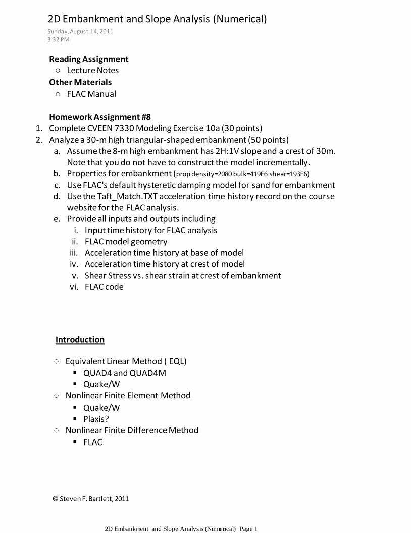
Homework Assignment #8Complete CVEEN 7330 Modeling Exercise 10a (30 points)1.

Assume the 8-m high embankment has 2H:1V slope and a crest of 30m. Note that you do not have to construct the model incrementally.

a.

Properties for embankment (prop density=2080 bulk=419E6 shear=193E6)b.Use FLAC's default hysteretic damping model for sand for embankmentc.Use the Taft_Match.TXT acceleration time history record on the course website for the FLAC analysis.

d.

Input time history for FLAC analysisi.FLAC model geometryii.Acceleration time history at base of modeliii.Acceleration time history at crest of modeliv.Shear Stress vs. shear strain at crest of embankmentv.FLAC codevi.

Provide all inputs and outputs includinge.

Analyze a 30-m high triangular-shaped embankment (50 points)2.

Introduction

2D Embankment and Slope Analysis (Numerical)Sunday, August 14, 2011

3:32 PM

2D Embankment and Slope Analysis (Numerical)


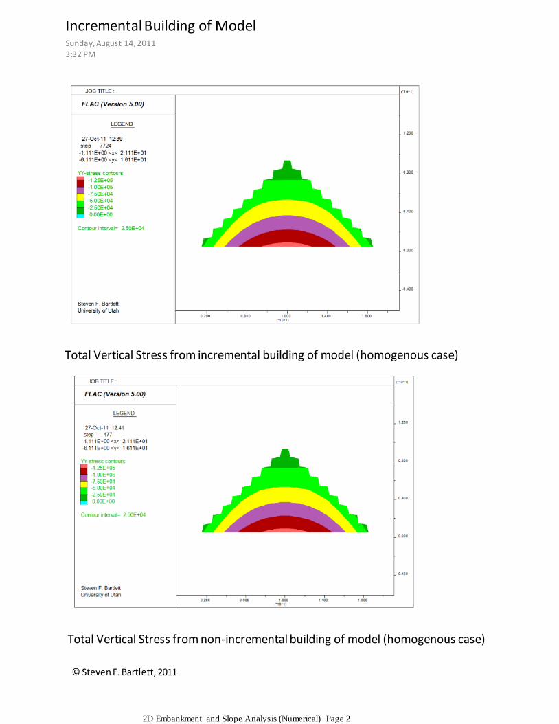
Total Vertical Stress from incremental building of model (homogenous case)

Total Vertical Stress from non-incremental building of model (homogenous case)

Incremental Building of ModelSunday, August 14, 20113:32 PM



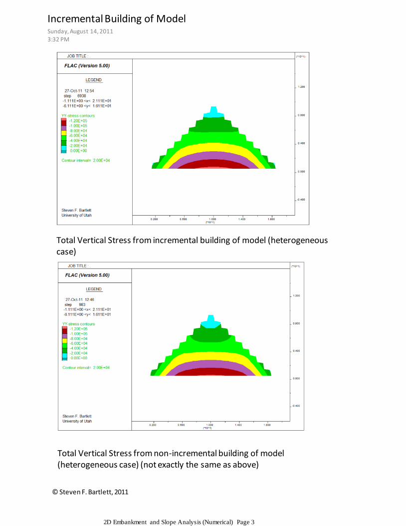
Total Vertical Stress from incremental building of model (heterogeneous case)

Total Vertical Stress from non-incremental building of model (heterogeneous case) (not exactly the same as above)

Incremental Building of ModelSunday, August 14, 2011

3:32 PM



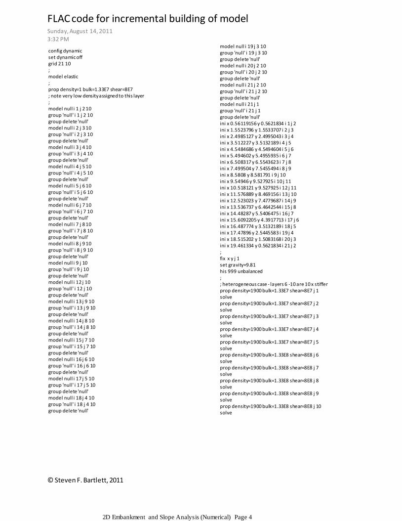
config dynamicset dynamic offgrid 21 10;model elastic;prop density=1 bulk=1.33E7 shear=8E7; note very low density assigned to this layer;model null i 1 j 2 10 group 'null' i 1 j 2 10 group delete 'null'model null i 2 j 3 10 group 'null' i 2 j 3 10 group delete 'null'model null i 3 j 4 10 group 'null' i 3 j 4 10 group delete 'null'model null i 4 j 5 10 group 'null' i 4 j 5 10 group delete 'null'model null i 5 j 6 10 group 'null' i 5 j 6 10 group delete 'null'model null i 6 j 7 10 group 'null' i 6 j 7 10 group delete 'null'model null i 7 j 8 10 group 'null' i 7 j 8 10 group delete 'null'model null i 8 j 9 10 group 'null' i 8 j 9 10 group delete 'null'model null i 9 j 10 group 'null' i 9 j 10 group delete 'null'model null i 12 j 10 group 'null' i 12 j 10 group delete 'null'model null i 13 j 9 10 group 'null' i 13 j 9 10 group delete 'null'model null i 14 j 8 10 group 'null' i 14 j 8 10 group delete 'null'model null i 15 j 7 10 group 'null' i 15 j 7 10 group delete 'null'model null i 16 j 6 10 group 'null' i 16 j 6 10 group delete 'null'model null i 17 j 5 10 group 'null' i 17 j 5 10 group delete 'null'model null i 18 j 4 10 group 'null' i 18 j 4 10 group delete 'null'

model null i 19 j 3 10 group 'null' i 19 j 3 10 group delete 'null'model null i 20 j 2 10 group 'null' i 20 j 2 10 group delete 'null'model null i 21 j 2 10 group 'null' i 21 j 2 10 group delete 'null'model null i 21 j 1 group 'null' i 21 j 1 group delete 'null'ini x 0.56119156 y 0.5621834 i 1 j 2ini x 1.5523796 y 1.5533707 i 2 j 3ini x 2.4985127 y 2.4995043 i 3 j 4ini x 3.512227 y 3.5132189 i 4 j 5ini x 4.5484686 y 4.5494604 i 5 j 6ini x 5.494602 y 5.4955935 i 6 j 7ini x 6.508317 y 6.5543623 i 7 j 8ini x 7.499504 y 7.5455494 i 8 j 9ini x 8.5808 y 8.581791 i 9 j 10ini x 9.54946 y 9.527925 i 10 j 11ini x 10.518121 y 9.527925 i 12 j 11ini x 11.576889 y 8.469156 i 13 j 10ini x 12.523023 y 7.4779687 i 14 j 9ini x 13.536737 y 6.4642544 i 15 j 8ini x 14.48287 y 5.5406475 i 16 j 7ini x 15.6092205 y 4.3917713 i 17 j 6ini x 16.487774 y 3.5132189 i 18 j 5ini x 17.47896 y 2.5445583 i 19 j 4ini x 18.515202 y 1.5083168 i 20 j 3ini x 19.461334 y 0.5621834 i 21 j 2;fix x y j 1set gravity=9.81his 999 unbalanced;; heterogeneous case - layers 6 -10 are 10 x stifferprop density=1900 bulk=1.33E7 shear=8E7 j 1solveprop density=1900 bulk=1.33E7 shear=8E7 j 2solveprop density=1900 bulk=1.33E7 shear=8E7 j 3solveprop density=1900 bulk=1.33E7 shear=8E7 j 4solveprop density=1900 bulk=1.33E7 shear=8E7 j 5solveprop density=1900 bulk=1.33E8 shear=8E8 j 6solveprop density=1900 bulk=1.33E8 shear=8E8 j 7solveprop density=1900 bulk=1.33E8 shear=8E8 j 8solveprop density=1900 bulk=1.33E8 shear=8E8 j 9solveprop density=1900 bulk=1.33E8 shear=8E8 j 10solve

FLAC code for incremental building of modelSunday, August 14, 2011

3:32 PM


Steven F. Bartlett, 2010

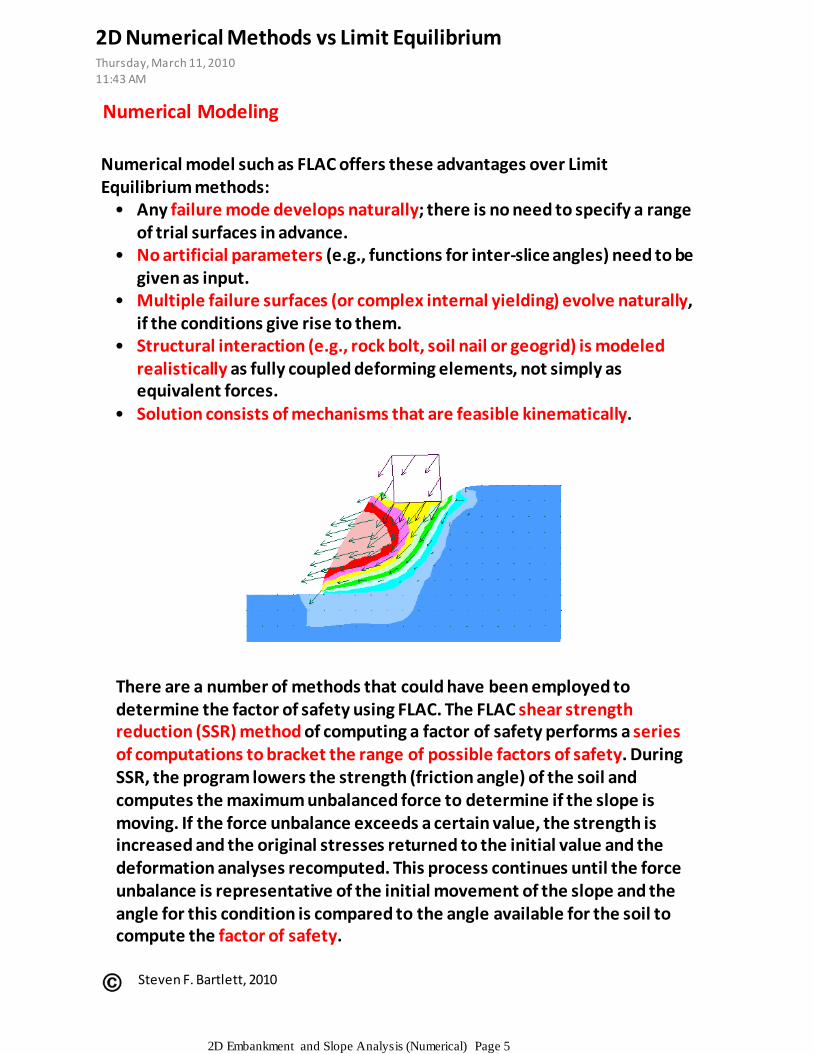
Numerical Modeling

Any failure mode develops naturally; there is no need to specify a range of trial surfaces in advance.

•

No artificial parameters (e.g., functions for inter-slice angles) need to be given as input.

•

Multiple failure surfaces (or complex internal yielding) evolve naturally, if the conditions give rise to them.

•

Structural interaction (e.g., rock bolt, soil nail or geogrid) is modeled realistically as fully coupled deforming elements, not simply as equivalent forces.

•

Solution consists of mechanisms that are feasible kinematically.•

Numerical model such as FLAC offers these advantages over Limit Equilibrium methods:

There are a number of methods that could have been employed to determine the factor of safety using FLAC. The FLAC shear strength reduction (SSR) method of computing a factor of safety performs a series of computations to bracket the range of possible factors of safety. During SSR, the program lowers the strength (friction angle) of the soil and computes the maximum unbalanced force to determine if the slope is moving. If the force unbalance exceeds a certain value, the strength is increased and the original stresses returned to the initial value and the deformation analyses recomputed. This process continues until the force unbalance is representative of the initial movement of the slope and the angle for this condition is compared to the angle available for the soil to compute the factor of safety.

2D Numerical Methods vs Limit EquilibriumThursday, March 11, 201011:43 AM



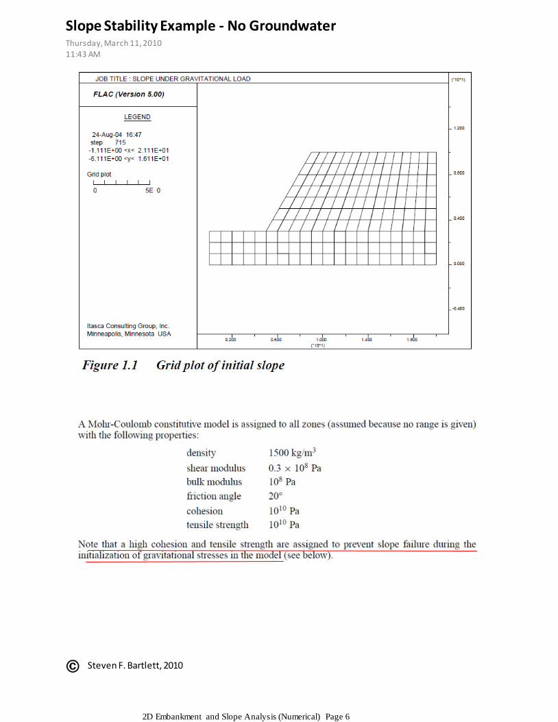
Slope Stability Example - No Groundwater Thursday, March 11, 2010

11:43 AM



Generating the slope

Slope Stability - No Groundwater (cont.)Thursday, March 11, 2010

11:43 AM



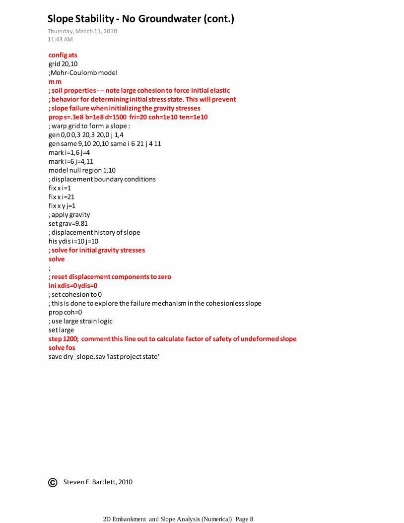
config atsgrid 20,10;Mohr-Coulomb modelm m; soil properties --- note large cohesion to force initial elastic; behavior for determining initial stress state. This will prevent; slope failure when initializing the gravity stressesprop s=.3e8 b=1e8 d=1500 fri=20 coh=1e10 ten=1e10; warp grid to form a slope :gen 0,0 0,3 20,3 20,0 j 1,4gen same 9,10 20,10 same i 6 21 j 4 11mark i=1,6 j=4mark i=6 j=4,11model null region 1,10; displacement boundary conditionsfix x i=1fix x i=21fix x y j=1; apply gravityset grav=9.81; displacement history of slopehis ydis i=10 j=10; solve for initial gravity stressessolve;; reset displacement components to zeroini xdis=0 ydis=0; set cohesion to 0; this is done to explore the failure mechanism in the cohesionless slopeprop coh=0; use large strain logicset largestep 1200; comment this line out to calculate factor of safety of undeformed slopesolve fossave dry_slope.sav 'last project state'


11:43 AM



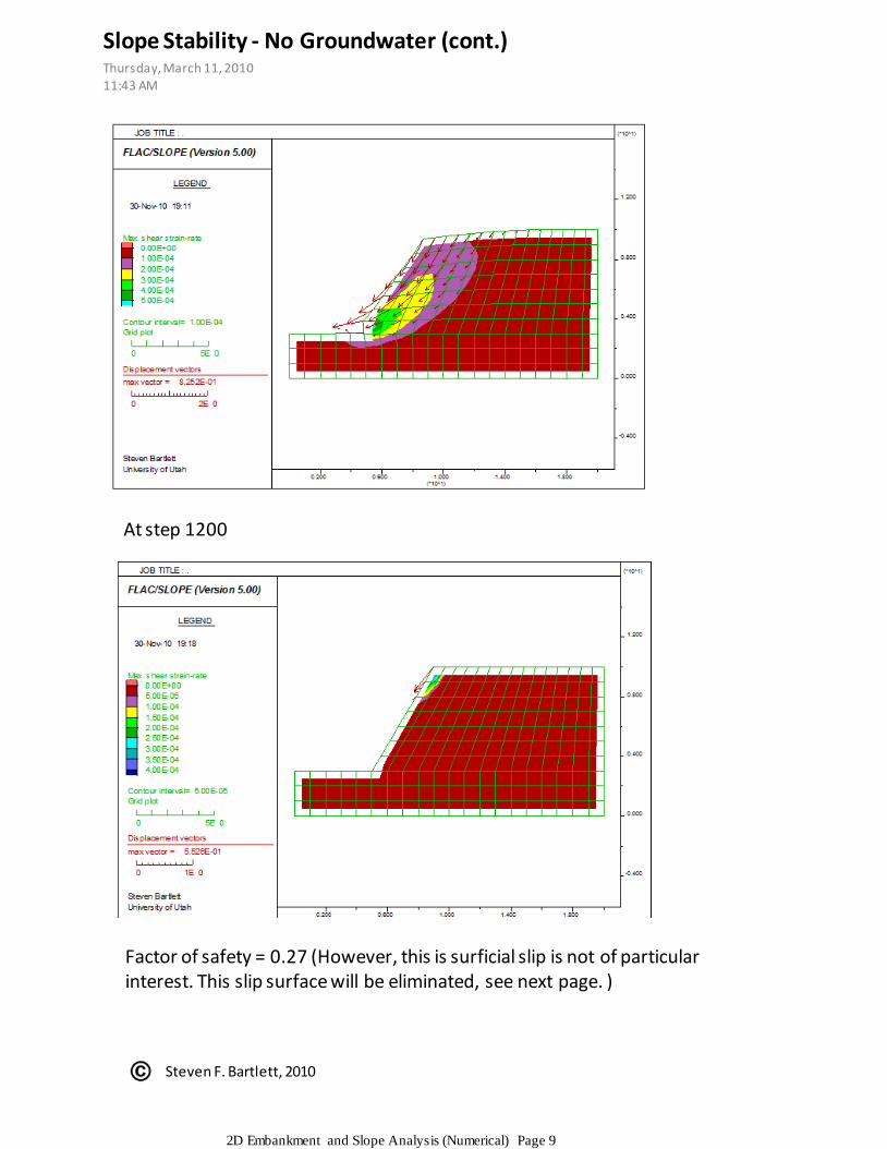
At step 1200

Factor of safety = 0.27 (However, this is surficial slip is not of particular interest. This slip surface will be eliminated, see next page. )

Slope Stability - No Groundwater (cont.)Thursday, March 11, 201011:43 AM



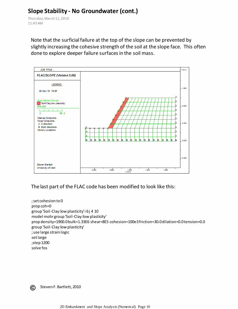
Note that the surficial failure at the top of the slope can be prevented by slightly increasing the cohesive strength of the soil at the slope face. This often done to explore deeper failure surfaces in the soil mass.

The last part of the FLAC code has been modified to look like this:

; set cohesion to 0prop coh=0group 'Soil-Clay:low plasticity' i 6 j 4 10 model mohr group 'Soil-Clay:low plasticity' prop density=1900.0 bulk=1.33E6 shear=8E5 cohesion=100e3 friction=30.0 dilation=0.0 tension=0.0 group 'Soil-Clay:low plasticity'; use large strain logicset large;step 1200solve fos


11:43 AM



Factor of safety = 0.58

(This is the true factor of safety of the slope for a rotation, slump failure.)


11:43 AM



A variety of finite element and finite difference computer programs are available for use in two- dimensional seismic site response analyses. The computer program QUAD4, originally developed by Idriss and his co-workers (Idriss et al., 1973) and recently updated as QUAD4M by Hudson et al. (1994), is among the most commonly used computer programs for two-dimensional site response analysis. QUAD4M uses an equivalent-liner soil model similar to the model used in SHAKE. Basic input to QUAD4M includes the two-dimensional soil profile, equivalent-linear soil properties, and the time history of horizontal ground motion. Time history of vertical ground motion may also be applied at the base of the soil profile. The base can be modeled as a rigid boundary, with design motions input directly at the base, or as a transmitting boundary which enables application of ground motions as hypothetical rock outcrop motions. With respect to the input soil properties, QUAD4M is very similar to SHAKE91. However, the ability to analyze two-dimensional geometry and the option for simultaneous base excitation with horizontal and vertical acceleration components make QUAD4M a more versatile analytical tool than SHAKE91.

A major difference between the QUAD4M and SHAKE91 equivalent-linear models is that the damping ratio in QUAD4M depends on the frequency of excitation or rate of loading. In QUAD4M, the equivalent-linear viscous damping ratio is used to fix the frequency dependent damping curve at the natural frequency of the soil deposit in order to optimize the gap between model damping and the damping ratio. A major drawback of QUAD4M is its limited pre- and post- processing capabilities. These limited capabilities make finite element mesh generation and processing and interpretation of the results difficult and time consuming. QUAD4M is available from the National Information Service for Earthquake Engineering (NISEE) at University Of California at Berkeley for a nominal cost.

Similar software is available commercially and can be purchased such as QUAKE/W. Generalized material property functions allow you to use any laboratory or published data. Three constitutive models are supported: a Linear-Elastic model, an Equivalent Linear model, and an effective stress Non-Linear model.

Pasted from <http://www.geo-slope.com/products/quakew.aspx>

2D Equivalent Linear Methods for Dynamic AnalysisWednesday, March 26, 2014

3:32 PM


http://www.geo-slope.com/products/quakew.aspx


Dynamic Loading and Boundary Conditions

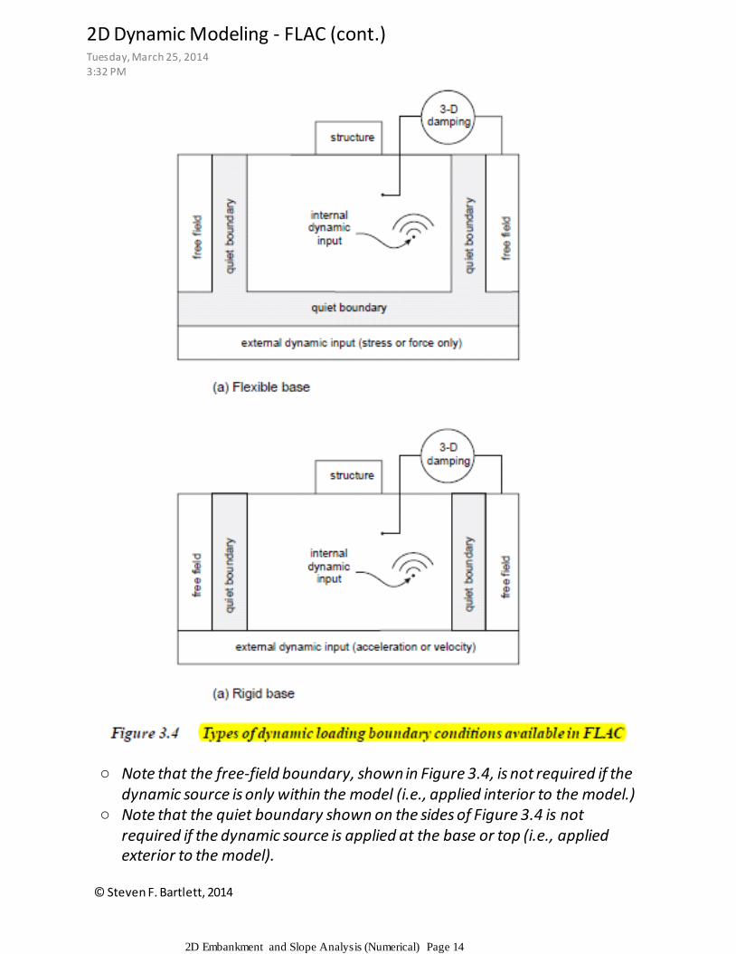
FLAC models a region of material subjected to external and/or internal dynamic loading by applying a dynamic input boundary condition at either the model boundary or at internal gridpoints. Wave reflections at model boundaries are minimized by specifying either quiet (viscous), free-field or three-dimensional radiation-damping boundary conditions. The types of dynamic loading andboundary conditions are shown schematically in Figure 3.4; each condition is discussed in the following sections.

Application of Dynamic Input

In FLAC, the dynamic input can be applied in one of the following ways:

(a) an acceleration history;(b) a velocity history;(c) a stress (or pressure) history; or(d) a force history.

Dynamic input is usually applied to the model boundaries (i.e., exterior) with the APPLY command. Accelerations, velocities and forces can also be applied to interior gridpoints by using the INTERIOR command.

2D Dynamic Modeling - FLAC (cont.)Tuesday, March 25, 2014

3:32 PM



Note that the free-field boundary, shown in Figure 3.4, is not required if the dynamic source is only within the model (i.e., applied interior to the model.)

○

Note that the quiet boundary shown on the sides of Figure 3.4 is not required if the dynamic source is applied at the base or top (i.e., applied exterior to the model).

○


3:32 PM



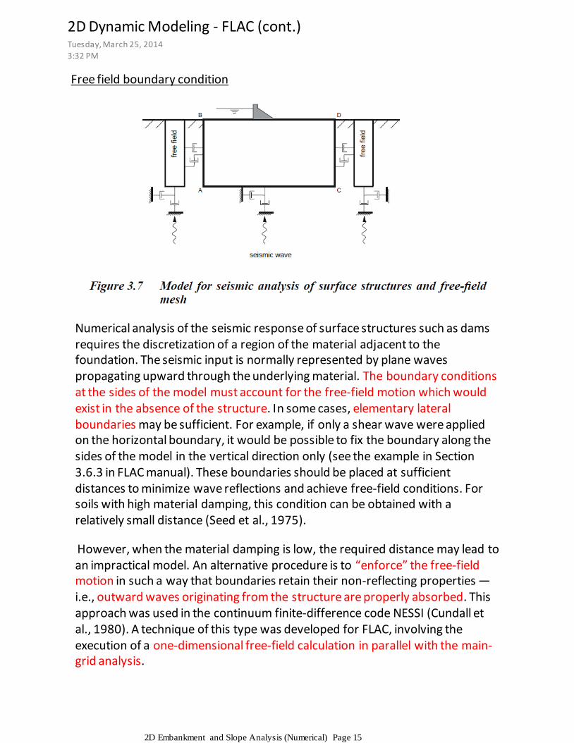
Free field boundary condition

Numerical analysis of the seismic response of surface structures such as dams requires the discretization of a region of the material adjacent to the foundation. The seismic input is normally represented by plane waves propagating upward through the underlying material. The boundary conditions at the sides of the model must account for the free-field motion which would exist in the absence of the structure. In some cases, elementary lateral boundaries may be sufficient. For example, if only a shear wave were applied on the horizontal boundary, it would be possible to fix the boundary along the sides of the model in the vertical direction only (see the example in Section 3.6.3 in FLAC manual). These boundaries should be placed at sufficient distances to minimize wave reflections and achieve free-field conditions. For soils with high material damping, this condition can be obtained with a relatively small distance (Seed et al., 1975).

However, when the material damping is low, the required distance may lead to an impractical model. An alternative procedure is to “enforce” the free-field motion in such a way that boundaries retain their non-reflecting properties —i.e., outward waves originating from the structure are properly absorbed. This approach was used in the continuum finite-difference code NESSI (Cundall et al., 1980). A technique of this type was developed for FLAC, involving the execution of a one-dimensional free-field calculation in parallel with the main-grid analysis.


3:32 PM



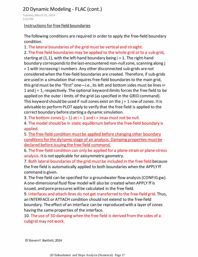
Instructions for free field boundaries

The following conditions are required in order to apply the free-field boundary condition.1. The lateral boundaries of the grid must be vertical and straight.2. The free field boundaries may be applied to the whole grid or to a sub-grid, starting at (1,1), with the left-hand boundary being i = 1. The right-hand boundary corresponds to the last-encountered non-null zone, scanning along j = 1 with increasing i numbers. Any other disconnected sub-grids are not considered when the free-field boundaries are created. Therefore, if sub-grids are used in a simulation that requires free-field boundaries to the main grid, this grid must be the “first” one—i.e., its left and bottom sides must be lines i= 1 and j = 1, respectively. The optional keyword ilimits forces the free field to be applied on the outer i limits of the grid (as specified in the GRID command). This keyword should be used if null zones exist on the j = 1 row of zones. It is advisable to perform PLOT apply to verify that the free field is applied to the correct boundary before starting a dynamic simulation.3. The bottom zones (j = 1) at i = 1 and i = imax must not be null.4. The model should be in static equilibrium before the free-field boundary is applied.5. The free-field condition must be applied before changing other boundary conditions for the dynamic stage of an analysis. Damping properties must be declared before issuing the free field command.6. The free-field condition can only be applied for a plane-strain or plane-stressanalysis. It is not applicable for axisymmetric geometry.7. Both lateral boundaries of the grid must be included in the free field becausethe free field is automatically applied to both boundaries when the APPLY ffcommand is given.8. The free field can be specified for a groundwater flow analysis (CONFIG gw).A one-dimensional fluid flow model will also be created when APPLY ff isissued, and pore pressures will be calculated in the free field.9. Interfaces and attach-lines do not get transferred to the free-field grid. Thus, an INTERFACE or ATTACH condition should not extend to the free-field boundary. The effect of an interface can be reproduced with a layer of zones having the same properties of the interface.10. The use of 3D damping when the free field is derived from the sides of a subgrid may not work.


3:32 PM



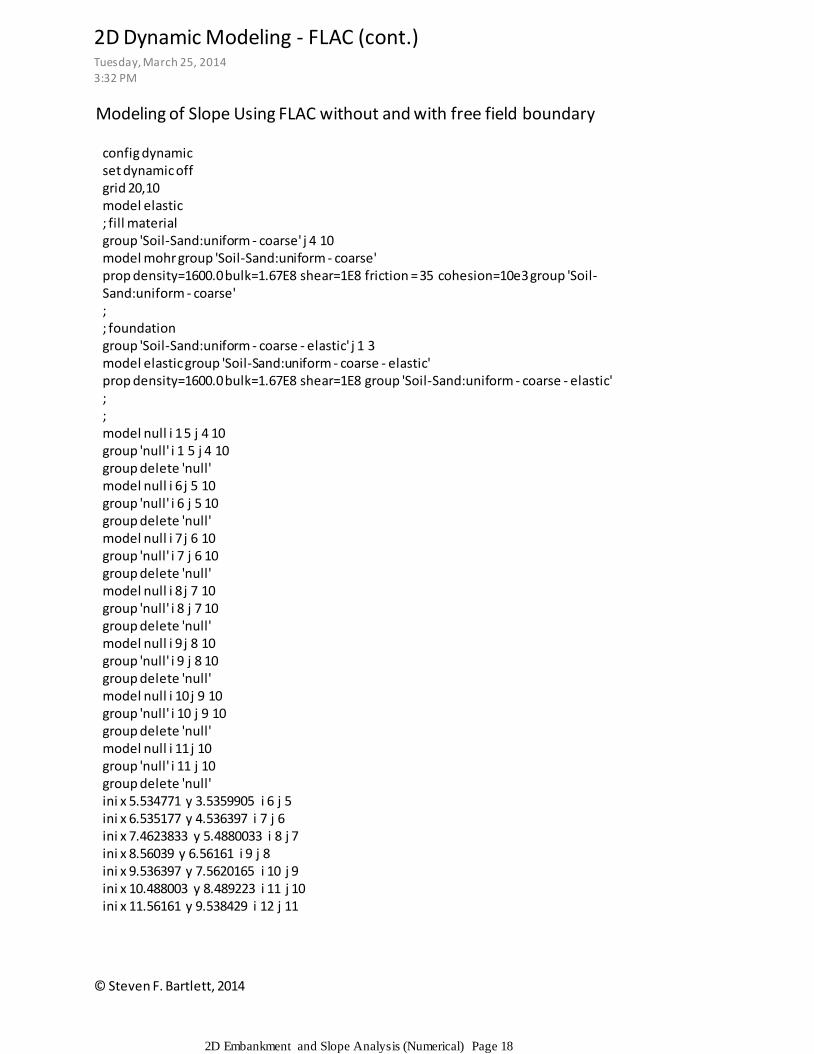
Modeling of Slope Using FLAC without and with free field boundary

config dynamicset dynamic offgrid 20,10model elastic; fill materialgroup 'Soil-Sand:uniform - coarse' j 4 10 model mohr group 'Soil-Sand:uniform - coarse' prop density=1600.0 bulk=1.67E8 shear=1E8 friction = 35 cohesion=10e3 group 'Soil-Sand:uniform - coarse';; foundationgroup 'Soil-Sand:uniform - coarse - elastic' j 1 3 model elastic group 'Soil-Sand:uniform - coarse - elastic' prop density=1600.0 bulk=1.67E8 shear=1E8 group 'Soil-Sand:uniform - coarse - elastic';;model null i 1 5 j 4 10group 'null' i 1 5 j 4 10group delete 'null'model null i 6 j 5 10group 'null' i 6 j 5 10group delete 'null'model null i 7 j 6 10group 'null' i 7 j 6 10group delete 'null'model null i 8 j 7 10group 'null' i 8 j 7 10group delete 'null'model null i 9 j 8 10group 'null' i 9 j 8 10group delete 'null'model null i 10 j 9 10group 'null' i 10 j 9 10group delete 'null'model null i 11 j 10group 'null' i 11 j 10group delete 'null'ini x 5.534771 y 3.5359905 i 6 j 5ini x 6.535177 y 4.536397 i 7 j 6ini x 7.4623833 y 5.4880033 i 8 j 7ini x 8.56039 y 6.56161 i 9 j 8ini x 9.536397 y 7.5620165 i 10 j 9ini x 10.488003 y 8.489223 i 11 j 10ini x 11.56161 y 9.538429 i 12 j 11


3:32 PM



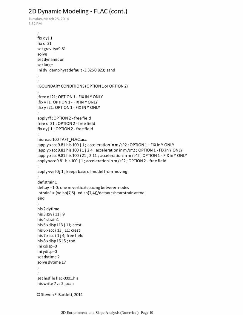
;fix x y j 1fix x i 21 set gravity=9.81solveset dynamic onset largeini dy_damp hyst default -3.325 0.823; sand;;; BOUNDARY CONDITIONS (OPTION 1 or OPTION 2);;free x i 21; OPTION 1 - FIX IN Y ONLY;fix y i 1; OPTION 1 - FIX IN Y ONLY;fix y i 21; OPTION 1 - FIX IN Y ONLY;apply ff ; OPTION 2 - free fieldfree x i 21 ; OPTION 2 - free fieldfix x y j 1 ; OPTION 2 - free field;his read 100 TAFT_FLAC.acc;apply xacc 9.81 his 100 j 1 ; acceleration in m /s^2 ; OPTION 1 - FIX in Y ONLY;apply xacc 9.81 his 100 i 1 j 2 4 ; acceleration in m /s^2 ; OPTION 1 - FIX in Y ONLY;apply xacc 9.81 his 100 i 21 j 2 11 ; acceleration in m /s^2 ; OPTION 1 - FIX in Y ONLYapply xacc 9.81 his 100 j 1 ; acceleration in m /s^2 ; OPTION 2 - free field;apply yvel 0 j 1 ; keeps base of model from moving;def strain1 ;deltay = 1.0; one m vertical spacing between nodes strain1 = (xdisp(7,5) - xdisp(7,4))/deltay ; shear strain at toeend;his 2 dytimehis 3 sxy i 11 j 9his 4 strain1his 5 xdisp i 13 j 11; cresthis 6 xacc i 13 j 11; cresthis 7 xacc i 1 j 4; free fieldhis 8 xdisp i 6 j 5 ; toeini xdisp=0ini ydisp=0set dytime 2solve dytime 17;;set hisfile flac-0001.hishis write 7 vs 2 ;accn


3:32 PM



acceleration applied to sides of model and base

acceleration applied to base with free field boundary on sides


3:32 PM




3:32 PM



BlankSunday, August 14, 2011

3:32 PM


2d embankment and slope analysis (numerical)bartlett/cveen7330/2d embankment and slope... ·...

Documents