2D Geometrical Transformations

• Tr anslation

- Moves points to new locations by adding translation amounts to the coordi-nates of the points

T

P(x,y)

P’ (x’,y’)

.

.

x′ = x + dx, y′ = y + dy or

x′y′

=

x

y

+

dx

dy

P′ = P + T

- To translate an object, translate every point of the object by the same amount

(translate only the endpoints of line segments - redrawing is required)

-2-

• Scaling

- Changes the size of the object by multiplying the coordinates of the points byscaling factors

x′ = x sx, y′ = y sy or

x′y′

=

sx

0

0

sy

x

y

, sx,sy > 0

P′ = S P

- Scale factors affect size as following:

* I f sx = sy uniform scaling

* I f sx ≠ sy nonuniform scaling

* I f sx, sy < 1, size is reduced, object moves closer to origin

* I f sx, sy > 1, size is increased, object moves further from origin

* I f sx = sy = 1, size does not change

-3-

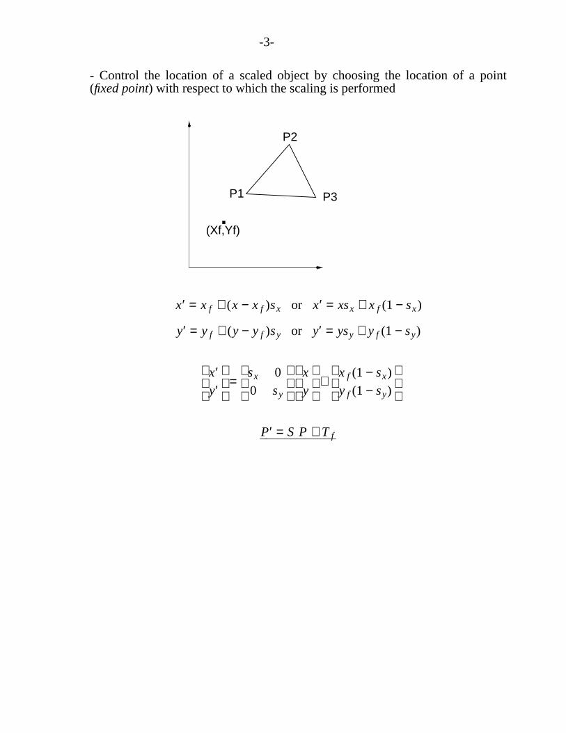
- Control the location of a scaled object by choosing the location of a point(fixed point) with respect to which the scaling is performed

(Xf,Yf)

P1

P2

P3

.

x′ = x f + (x − x f )sx or x′ = xsx + x f (1 − sx)

y′ = y f + (y − y f )sy or y′ = ysy + y f (1 − sy)

x′y′

=

sx

0

0

sy

x

y

+

x f (1 − sx)

y f (1 − sy)

P′ = S P+ T f

-4-

• Rotation

- Rotates points by an angle�

about origin (�>0: counterclockwise rotation)

- From ABP triangle:

cos( � ) = x/r or x = rcos( � )sin( � ) = y/r or y = rsin( � )

- From ACP′ triangle:

cos( � + �) = x′/r or x′ = rcos( � + �

) = rcos( � )cos(�) − rsin( � )sin(

�)

sin( � + �) = y′/r or y′ = rsin( � + �

) = rcos( � )sin(�) + rsin( � )cos(

�)

- From the above equations we have:

x′ = xcos(�) − ysin(

�), y′ = xsin(

�) + ycos(

�) or

x′y′

=

cos(�)

sin(�)

−sin(�)

cos(�)

x

y

P′ = R P

- To rotate an object, rotate every point of the object by the same amount

-5-

(rotate only the endpoints of line segments - redrawing is required)

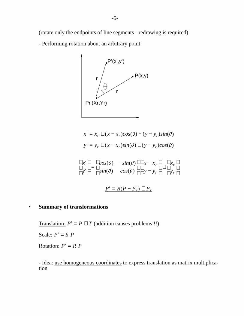
- Performing rotation about an arbitrary point

.r

r

P’(x’,y’)

P(x,y)

(Xr,Yr)Pr

..

x′ = xr + (x − xr )cos( � ) − (y − yr )sin( � )

y′ = yr + (x − xr )sin( � ) + (y − yr )cos( � )

x′y′

=

cos( � )

sin( � )

−sin( � )

cos( � )

x − xr

y − yr

+

xr

yr

P′ = R(P − Pr ) + Pr

• Summary of transformations

Translation:P′ = P + T (addition causes problems !!)

Scale:P′ = S P

Rotation:P′ = R P

- Idea: use homogeneous coordinates to express translation as matrix multiplica-tion

-6-

• Homogeneous coordinates (projective space)

- Idea: add a third coordinate: (x, y) --> (xh, yh, w)

- Homogenize (xh, yh, w):

x =xh

w, y =

yh

w, w ≠ 0

- In general: (x, y) --> (xw, yw, w) (i.e., xh=xw, yh=yw)

- w can assume any value (w ≠ 0), for example,w = 1:

(x, y) − − > (x, y, 1) (no division is required when you homogenize !!)

(x, y) − − > (2x, 2y, 2) (division is required when you homogenize !!)

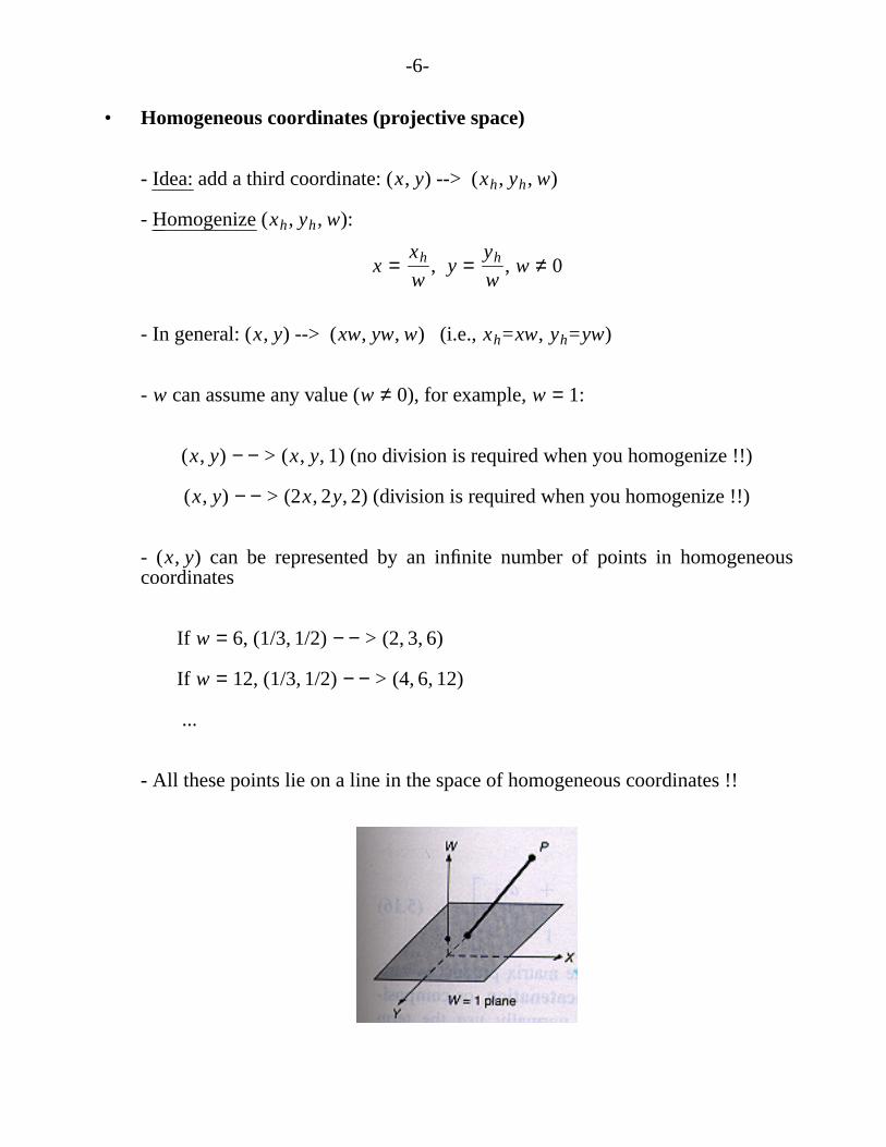
- (x, y) can be represented by an infinite number of points in homogeneouscoordinates

If w = 6, (1/3,1/2) − − > (2, 3, 6)

If w = 12, (1/3,1/2) − − > (4, 6, 12)

...

- All these points lie on a line in the space of homogeneous coordinates !!

-7-

• Tr anslation using homogeneous coordinates

x′y′1

=

1

0

0

0

1

0

dx

dy

1

x

y

1

(Verification:x′ = 1x + 0y + 1dx = x + dx)

(Verification:y′ = 0x + 1y + 1dy = y + dy)

(Homogenize: divide by 1 !!)

P′ = T(dx, dy) P

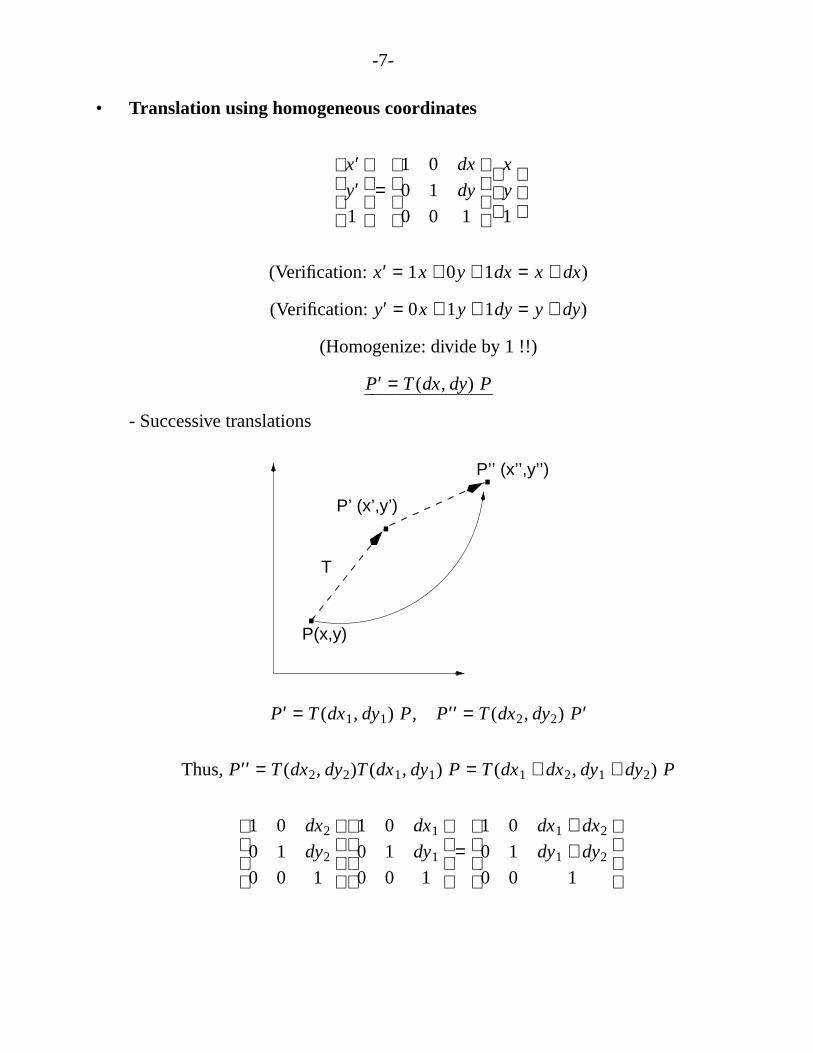
- Successive translations

T

P(x,y).

.P’ (x’,y’)

P’’ (x’’,y’’).

P′ = T(dx1, dy1) P, P′′ = T(dx2, dy2) P′

Thus,P′′ = T(dx2, dy2)T(dx1, dy1) P = T(dx1 + dx2, dy1 + dy2) P

1

0

0

0

1

0

dx2

dy2

1

1

0

0

0

1

0

dx1

dy1

1

=

1

0

0

0

1

0

dx1 + dx2

dy1 + dy2

1

-8-

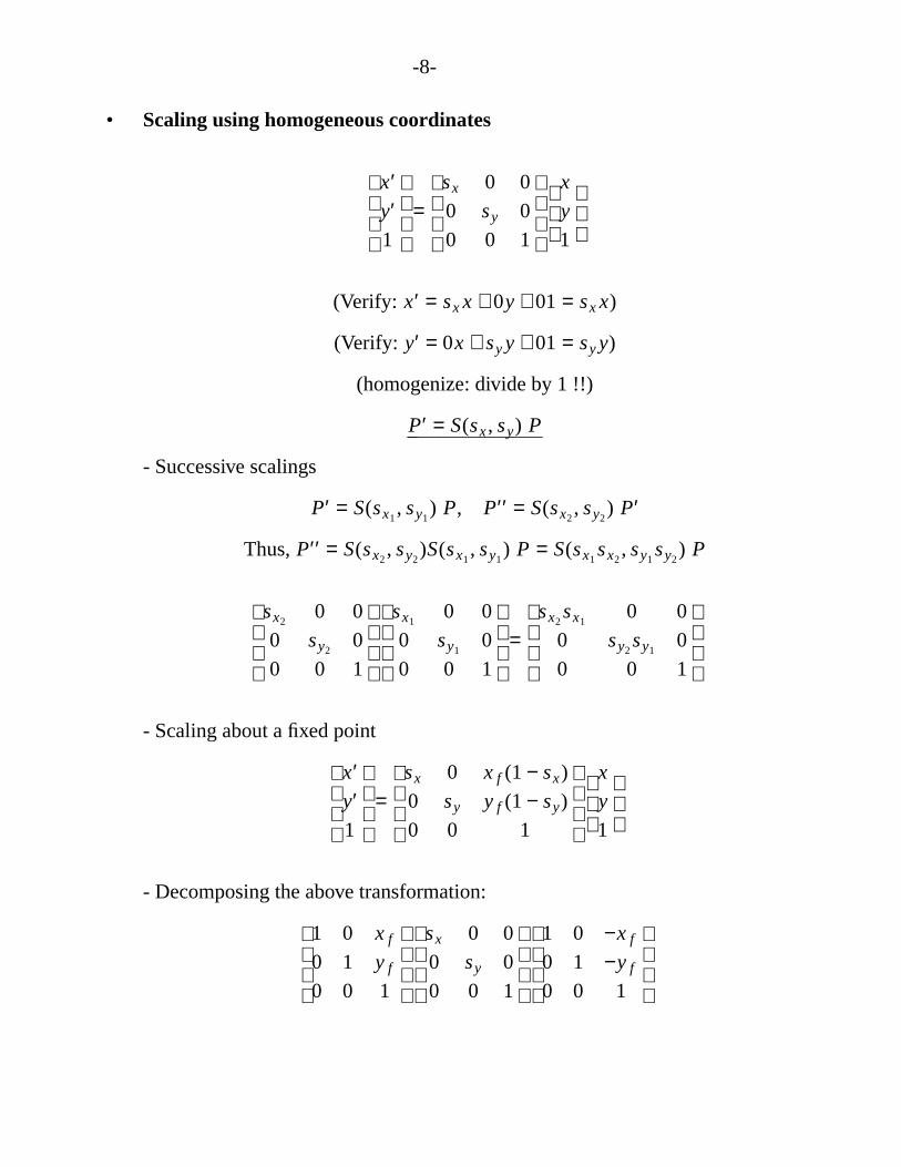
• Scaling using homogeneous coordinates

x′y′1

=

sx

0

0

0

sy

0

0

0

1

x

y

1

(Verify: x′ = sx x + 0y + 01 = sx x)

(Verify: y′ = 0x + syy + 01 = syy)

(homogenize: divide by 1 !!)

P′ = S(sx, sy) P

- Successive scalings

P′ = S(sx1, sy1

) P, P′′ = S(sx2, sy2

) P′

Thus,P′′ = S(sx2, sy2

)S(sx1, sy1

) P = S(sx1sx2

, sy1sy2

) P

sx2

0

0

0

sy2

0

0

0

1

sx1

0

0

0

sy1

0

0

0

1

=

sx2sx1

0

0

0

sy2sy1

0

0

0

1

- Scaling about a fixed point

x′y′1

=

sx

0

0

0

sy

0

x f (1 − sx)

y f (1 − sy)

1

x

y

1

- Decomposing the above transformation:

1

0

0

0

1

0

x f

y f

1

sx

0

0

0

sy

0

0

0

1

1

0

0

0

1

0

−x f

−y f

1

-9-

• Rotation using homogeneous coordinates

x′y′1

=

cos( � )

sin( � )

0

−sin( � )

cos( � )

0

0

0

1

x

y

1

P′ = R( � ) P

- Successive rotations

P′ = R( � 1) P, P′′ = R( � 2) P′

Thus,P′′ = R( � 1)R( � 2) P = R( � 1 + � 2) P

- Rotation about an arbitrary point

x′y′1

=

cos( � )

sin( � )

0

−sin( � )

cos( � )

0

xr (1 − cos( � )) + yr sin( � )

yr (1 − cos( � )) − xr sin( � )

1

x

y

1

- Decomposing the above transformation:

1

0

0

0

1

0

xr

yr

1

cos( � )

sin( � )

0

−sin( � )

cos( � )

0

0

0

1

1

0

0

0

1

0

−xr

−yr

1

-10-

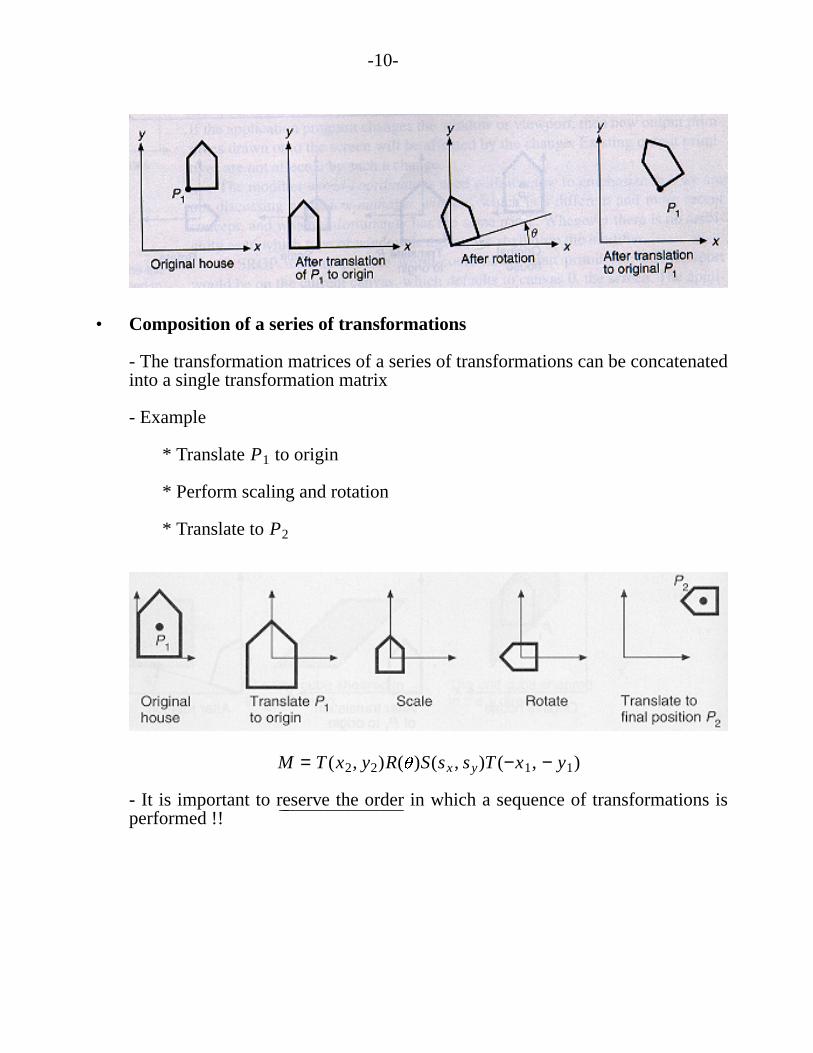
• Composition of a series of transformations

- The transformation matrices of a series of transformations can be concatenatedinto a single transformation matrix

- Example

* TranslateP1 to origin

* Perform scaling and rotation

* Translate toP2

M = T(x2, y2)R( � )S(sx, sy)T(−x1, − y1)

- It is important to reserve the order in which a sequence of transformations isperformed !!

-11-

• General form of transformation matrix

x′y′1

=

a11

a21

0

a12

a22

0

a13

a23

1

x

y

1

- Representing a sequence of transformations as a single transformation matrixis more efficient

x′ = a11x + a12y + a13

y′ = a21x + a22y + a23

only 4 multiplications and 4 additions

• Similarity transf ormations

- Inv olve rotation, translation, scaling

• Rigid-body transformations

- Inv olve only translations and rotations

- Preserve angles and lengths

- General form of a rigid-body transformation matrix

x′y′1

=

r11

r21

0

r12

r22

0

tx

ty

1

x

y

1

-12-

- Properties

* The upper 2x2 submatrix is ortonormal

u1 = (r11, r12), u2 = (r21, r22)

u1. u1 = ||u1||2 = r112 + r12

2 = 1

u2. u2 = ||u2||2 = r212 + r22

2 = 1

u1. u2 = r11r21 + r12r22 = 0

- Example:

cos( � )

sin( � )

0

−sin( � )

cos( � )

0

0

0

1

u1. u1 = cos( � )2 + sin(− � )2 = 1

u2. u2 = cos( � )2 + sin( � )2 = 1

u1. u2 = cos( � )sin( � ) − sin( � )cos( � ) = 0

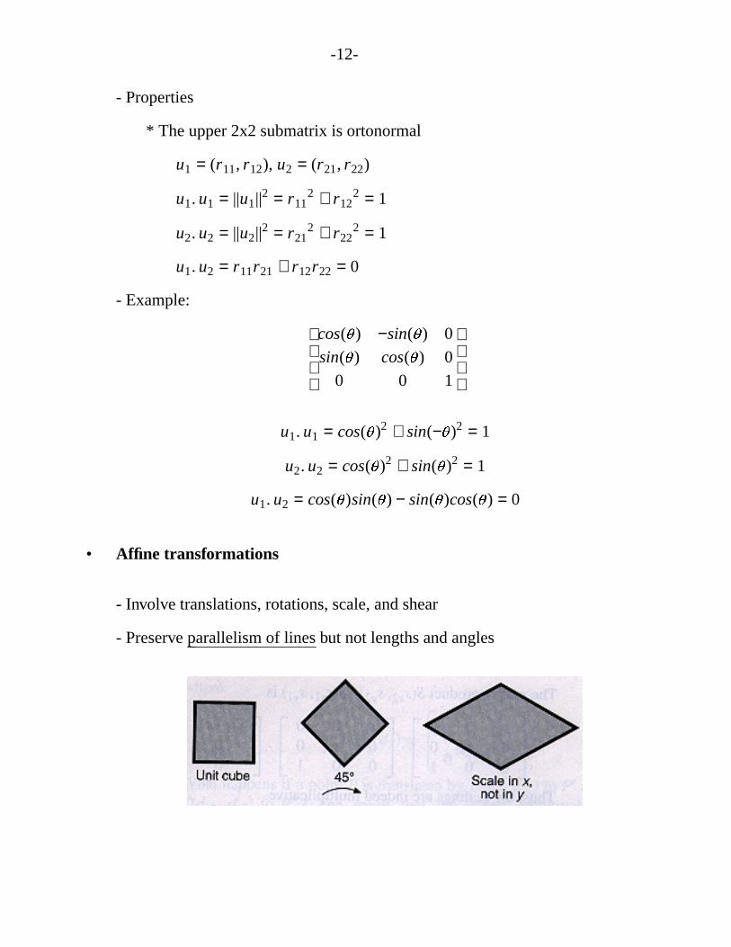
• Affine transformations

- Inv olve translations, rotations, scale, and shear

- Preserve parallelism of lines but not lengths and angles

-13-

• Shear transformations

- Changes the shape of the object.

- Shear along the x-axis:

x′ = x + ay, y′ = y

SHx =

1

0

0

a

1

0

0

0

1

- Shear along the y-axis:

x′ = x, y′ = bx + y

SHy =

1

b

0

0

1

0

0

0

1