Comput Mech (2016) 58:411–422DOI 10.1007/s00466-016-1300-4

ORIGINAL PAPER

2D–3D hybrid stabilized finite element method for tsunami runupsimulations

S. Takase1 · S. Moriguchi2 · K. Terada2 · J. Kato1 ·T. Kyoya1 · K. Kashiyama3 · T. Kotani1

Received: 16 January 2015 / Accepted: 5 May 2016 / Published online: 21 May 2016© Springer-Verlag Berlin Heidelberg 2016

Abstract This paper presents a two-dimensional (2D)–three-dimensional (3D) hybrid stabilized finite elementmethod that enables us to predict a propagation process oftsunami generated in a hypocentral region, which rangesfrom offshore propagation to runup to urban areas, withhigh accuracy and relatively low computational costs. To bemore specific, the 2D shallow water equation is employedto simulate the propagation of offshore waves, while the 3DNavier–Stokes equation is employed for the runup in urbanareas. The stabilized finite element method is utilized fornumerical simulations for both of the 2Dand 3Ddomains thatare independently discretized with unstructured meshes. Themulti-point constraint and transmission methods are appliedto satisfy the continuity of flow velocities and pressures atthe interface between the resulting 2D and 3D meshes, sinceneither their spatial dimensions nor node arrangements areconsistent. Numerical examples are presented to demonstratethe performance of the proposed hybrid method to simulatetsunami behavior, including offshore propagation and runupto urban areas, with substantially lower computation costs incomparison with full 3D computations.

B S. Takasetakase@irides.tohoku.ac.jp

1 Department of Civil and Environmental Engineering,Tohoku University, Aza-Aoba 6-6, Aramaki, Aoba-ku,Sendai 980-0845, Japan

2 International Research Institute of Disaster Science,Tohoku University, Aza-Aoba 468-1, Aramaki, Aoba-ku,Sendai 980-0845, Japan

3 Department of Civil and Environmental Engineering,Chuo University, Kasuga 1-13-27, Bunkyou-ku,Tokyo 112-8521, Japan

Keywords Stabilized finite element method · 2D–3Dhybrid method · MPC · Tsunami

1 Introduction

There is no end to inundation disasters caused by tsunami,storm surges, floods and so on. Since these disasters threatenpeople’s lives and destroy their properties, it is quite impor-tant to accurately predict the flooded areas by some kindof method. Although model experiments were mainly con-ducted in the past, recent years have seen a replacement bynumerical simulation in predicting flooded areas as well asthe extent of damage. This fact is due to both the improvedperformance of computer hardware and accuracy of numer-ical analysis techniques, as well as the development andwidespread use of detailed topographic and residential digitalmaps [1–4].

For simulation of tsunami runup, in particular, whichrequires covering a broad range of tsunami behavior fromoffshore propagation to runup to land, numerical analysismethods based on the shallow water theory with an cartesiangrid are widely used because of their technical simplic-ity and low computation costs [5,6]. However, a tsunamirunup behavior in urban areas reveals three-dimensional(3D) characteristics in general, and involves highly com-plex free-surface flows that are caused by the effects ofstructures and landscapes, it is obviously inappropriate toapply the two-dimensional (2D) shallow water approxima-tion for the purpose of evaluating the fluid force actingon structures. Therefore, numerical analyses based on theNavier–Stokes equation [7], which are applicable for 3Dcomplex free-surface flows, have become common in recentyears. Nonetheless, 3D simulations from offshore to runupareas inevitably require a significant increase in the degree

123

412 Comput Mech (2016) 58:411–422

of freedom (DOF), making this approach seem unrealistic interms of computational costs.

To overcome this problem, several 2D–3Dhybridmethodshave been proposed in the literature [8–11]. Those meth-ods are designed to enable us to perform 3D analyses inthe regions where 2D approximation is impossible, such asaround tsunami breakwaters or buildings, while reflectingshallow water analysis results. However, since most of themethods proposed in the past are on the basis of using carte-sian grids for both the 2D and 3D regions, the exact geometryof structures cannot be reflected in the numerical analysisand, as a result, desired accuracy is not obtained in evalu-ating fluid forces acting on the structures. To evaluate thefluid forces properly, the surrounding flow regimes shouldbe accurately analyzed, and to do this, approaches with anboundary-fitted grid capable of representing the shapes ofstructures must be employed.

In this study, employing the stabilized finite elementmethod (FEM) to accurately evaluate the fluid forces act-ing on structures, we propose its 2D–3D hybrid versionthat enables us predict a propagation process of tsunami,which ranges from offshore propagation to runup to urbanareas, with high accuracy and relatively low computationalcosts. For a numerical analysis of offshore wave propagation,the 2D shallow water equation is used and the StreamlineUpwind Petrov Galerkin (SUPG) method is employed fortheir finite element discretization. For an analysis tsunamirunup, the 3D Navier-Strokes equation is discreteized by theSUPG/pressure stabilizing Petrov Galerkin (PSPG) methodand the VOF method is employed to capture the free-surfaceevolutions. Since the proposed method allows us to utilizeunstructured grids with triangular and tetrahedral elementsfor the 2D and 3D regions, respectively, possible errorscaused by the approximation of shape representation canbe reduced to some extent. For stable numerical analyseswith the stabilized FEM, the implicit scheme is employedfor the temporal discretization of both the 2D shallow waterand 3D Navier–Stokes equations. The respectively deriveddiscretized 2D and 3D equations are solved simultaneouslywith the help of the multiple point constraint (MPC) tech-nique [12] to impose the continuity conditions of both thevelocities and pressures at the interface between the 2D and3D domains. To the best of the authors’ knowledge, therehave been no reports with the same approach. Even if com-mercial software is utilized with MPCs, care is necessary tosatisfy the continuity of the velocity in the vertical direction.Needless to say, the node arrangements at their interface neednot be conformable.

In the subsequent sections, after providing the governingequations and their discretization, we explain in detail theMPC and transmission techniques implemented into the 2D–3D hybrid-type stabilized FEM that is the combination ofthe standard stabilized FEMs for shallow water and Navier–

Stokes flows. A simple numerical example is presented toverify the capability of the implemented MPC function toimpose the continuity conditions at the 2D–3D interface. Theperformance of the proposed method is also demonstratedby estimating the disaster reduction effect of a submergedbreakwater in an urban area attacked by tsunami runup.

2 Stablized finite element method

After the governing equations for the 3DNavier–Stokes flowfield and the 2D shallow water flow field are presented,the stabilized finite element method (FEM) is applied toobtain the corresponding discretized equations. The Crank–Nicolson method is employed for temporal discretization forthese governing equations.TheVOFmethod that is employedto capture the 3D free-surface flow is also outlined.

2.1 Governing equations

Assuming an incompressible viscous fluid, we employ thefollowing set of the Navier–Stokes equation and continuityequation to describe the 3D flow field in an urban area:

ρ(∂u

∂t+ u · ∇u − f

)− ∇ · σ (u, p) = 0 (1)

∇ · u = 0 (2)

where ρ, u = [uns, vns, wns]T, p, f and σ are the fluid massdensity, flow velocity vector, pressure, body force vector, andstress tensor, respectively. Assuming a Newtonian fluid, thestress field is determined by the following constitutive law:

σ = −p I + 2με(u) (3)

Here, μ is the viscosity coefficient and ε(u) is the rate ofdeformation tensor defined in the equation below:

ε(u) = 1

2

(∇u + (∇u)T

)(4)

The shallow water approximation is applied for thetsunami behavior of offshore wave propagations so that the2D shallow water equation can be used up to the onset ofrunup. For the non-conserved system, the set of the shallowwater equation is given as

∂U∂t

+ Aα

∂U∂xα

− ∂

∂xα

(Kαβ

∂U∂xβ

)− R = 0 (5)

where the summation convention is applied for α, β = 1, 2.Here, we have definedU = [h, usw, vsw]T as the set of non-conserved variables, in which h is the total water height, andusw and vsw are the components of the average flow velocity;

123

Comput Mech (2016) 58:411–422 413

zb

h

xy

z

usw

base surface

Fig. 1 Coordinate system for shallow-water problem

see Fig. 1. Also, Aα is the matrix to form the advection termsuch that

A1 =⎡⎣usw h 0g usw 00 0 usw

⎤⎦ , A2 =

⎡⎣

vsw 0 h0 vsw 0g 0 vsw

⎤⎦ (6)

and Kαβ and R are defined respectively as:

K 11 = ν

⎡⎣0 0 00 2 00 0 1

⎤⎦ , K 12 = ν

⎡⎣0 0 00 0 00 1 0

⎤⎦ (7)

K 21 = ν

⎡⎣0 0 00 0 10 0 0

⎤⎦ , K 22 = ν

⎡⎣0 0 00 1 00 0 2

⎤⎦ (8)

R =

⎡⎢⎢⎢⎣

0

−g∂zb∂x

− u∗husw

−g∂zb∂y

− u∗h

vsw

⎤⎥⎥⎥⎦ , u∗ = gn2

√u2sw + v2sw

h1/3(9)

where g, ν, zb, and n respectively represent the accelerationdue to gravity, the eddy viscosity coefficient, the altitude ofthe bottom surface, and theManning’s roughness coefficient.

2.2 Stabilized finite element method

The application of the SUPG/PSPG method [13,14] to thegoverning equations for the 3D flow field, Eqs.(1) and (2),yields the following discretized equation of the stabilizedFEM.

ρ

∫

Ωns

wh · ρ

(∂uh

∂t+ uh · ∇uh − f

)dΩ

+∫

Ωns

ε(wh) : σ (uh, ph) dΩ +∫

�ns

qh∇ · uh dΩ

+nel∑e=1

∫

Ωens

{τ nssupgu

h · ∇wh + τ nspspg1

ρ∇q

}

×{ρ

(∂uh

∂t+ uh · ∇uh − f

)− ∇ · σ (uh, ph)

}dΩ

+nel∑e=1

∫

Ωens

τ nscont∇ · whρ∇ · uh dΩ = 0 (10)

where Ωns ∈ R3 is the 3D analysis domain for the Navier–

Stokes equation. Here, uh and ph respectively represent thefinite element (FE) approximations of the velocity and pres-sure fields, while wh and qh are the approximations of theweighting functions with respect to the momentum equationand the continuity equation, respectively. Also, the fourthterm of this discretized equation arises from the SUPG andPSPG methods, which are respectively introduced to stabi-lize the advection-induced unstable behavior and to suppressthe pressure oscillation, and the fifth term is introduced forshock-capturing [15] to avoid the numerical instability of freesurfaces. These stabilization terms are evaluated element-wise with nel being the number of elements, and τ nssupg, τ

nspspg

and τ nscont involves the stabilization parameters, which arerespectively defined as follows:

τ nssupg =[(

2

t

)2

+(2||uh ||he

)2

+(4ν

h2e

)2]− 1

2

(11)

τ nspspg = τ nssupg (12)

τcont = he2

||uh ||ξ (Ree) (13)

Ree = ||uh ||he2ν

(14)

ξ (Ree) ={ Ree

3, Ree ≤ 3

1, Ree > 3(15)

where t, he, ν, and Ree are the time increment, the char-acteristic element length, the kinematic viscosity coefficient,and the Reynolds number of the element, respectively.

On the other hand, the shallow water Eq. (5) can be dis-cretized with the SUPG method [16] as

∫

Ωsw

Uh∗ ·(

∂Uh

∂t+ Ah

α

∂Uh

∂xα

− Rh

)d�

+∫

Ωsw

(∂Uh∗∂xα

)·(K h

αβ

∂Uh∗∂xβ

)dΩ

+nel∑e=1

∫

Ωesw

τ swsupg

(Ah

β

)T (∂Uh∗∂xβ

)

·(

∂Uh

∂t+ Ah

α

∂Uh

∂xα

− Rh

)dΩ

+nel∑e=1

∫

Ωesw

τ swcont

(∂Uh∗∂xα

)·(

∂Uh

∂xα

)= 0 (16)

123

414 Comput Mech (2016) 58:411–422

where Ωsw ∈ R2 represents the analysis domain of the 2D

shallow water equation. Here,Uh, Ahα, K h

αβ and Rhα (α, β =

1, 2) contain the FE approximations of the velocity fieldsusw and vsw, and Uh∗ is the FE approximation of U∗, whichis theweighting function ofU . The third termof this equationarises from the SUPGmethod to stabilize the unstable behav-ior due to the dominance of advection, and the fourth termis introduced for shock-capturing term [17] to avoid numeri-cal instability of free surfaces. The stabilization parameters,τ swsupg and τ swcont, in these terms are respectively defined as

τ swsupg =⎡⎣

(2

t

)2

+(2||uh ||he

)2

+(4ν

h2e

)2⎤⎦

− 12

(17)

τ swcont = he2

||uh || z (18)

with

z ={ κk

3, κk ≤ 3

1, κk > 3(19)

Here, we have introduced the following definitions: ||uh || =√||uhsw||2 + c2, c = √gh, κk = ||uh ||he/ν and uhsw =

[usw, vsw]T .We impose the MPC on the nodal solutions of the FE

equations, resulting from (10) or (16), so that the continuityconditions of flow velocities and pressures must be satisfiedat the 2D–3D interface. The details are presented in the nextsection.

2.3 VOF method for free-surface capturing

There are two kinds of approaches to determine the geom-etry of a free surface that is an interface between the gas(air) and the liquid (water) whose 3d motions are governedby Eqs. (1) and (2). One of them is the class of interface-capturing approaches that employ the Euler technique witha fixed mesh, and the other is the class of interface-trackingapproaches that take the Lagrange technique with a movingmesh. In this study,we employ theVOFmethod,which is oneof the interface-capturingmethods, since our target problemsinvolve breaking waves that have complex free surfaces.

In the VOF method, the movement of a free-surface isdefined as the time-variation of the VOF or interface functionφ that is governed by the following advection equation:

∂φ

∂t+ u · ∇φ = 0 (20)

where φ takes 0.0 for gas and 1.0 for liquid, while the inter-mediate values represent their interface. With the values ofthe VOF function, the density ρ and the viscosity coefficientμ at any point of the fluid can be expressed as

ρ = ρlφ + ρg(1 − φ) (21)

μ = μlφ + μg(1 − φ) (22)

where ρl and ρg are the densities of liquid (water) and gas(air), and μl and μg are the corresponding viscosity coeffi-cients.

By applying the stabilized FE approximation with theSUPG method [15] to the governing Eq. (20) for the VOFfunction, we obtain the discretized equation as follows:

∫

Ωns

φh∗(

∂φh

∂t+ uh · ∇φ

)dΩ

+nel∑e=1

∫

Ωens

τφ uh · ∇φh∗(

∂φh

∂t+ uh · ∇φh

)dΩ

+n∑

e=1

∫

Ωens

τIC ∇φh∗ · ∇φh dΩ = 0 (23)

where φh and φh∗ are the FE approximations of the VOFfunction φ and its weighting function. Also, τφ and τIC arethe stabilization parameters defined by

τφ =[(

2

t

)2

+(2||uh ||he

)2]− 1

2

(24)

τIC = he2

||uh || (25)

The last term of Eq. (23) is introduced to suppressthe numerical undershoots and overshoots of the inter-face function around the interface. The so-called interface-sharpening/mass-conservation algorithm proposed in [15]enables us to not only sharpen the interface, but also sat-isfy the conservation of mass for the fluids by appropriatelyselecting the stabilization parameter Eq. (25).

On the interface between the 2D and 3D domain, the posi-tion of the free surface on its 3D domain side is equalizedto the water height of its 2D domain side, which is the solu-tion of the shallow water equation. Then, the VOF value ofthe free surface is set at 0.5 so that the VOF values alongthe interface curve are determined accordingly. Note thatthe advection velocity uh in Eq. (23) is the solution of theFE equation obtained by integrating Eqs.(10) or (16) withthe help of MPC method, which is explained the next sec-tion.

123

Comput Mech (2016) 58:411–422 415

3 Techniques for 2D-3D hybrid versionof stabilized FEM

We have to simultaneously solve the 2D shallow water equa-tion for tsunami propagations of offshore areas (Ωsw) andthe 3D Navier–Stokes equation (and continuity equation) fortsunami runup inurban areas (Ωns). Since the implicitmethodis adopted for temporal discretization, the 2D-3D hybrid sta-bilized FEM proposed in this study can be established by theintegration of (10) or (16) with an appropriate way to satisfythe continuity conditions of flow velocities and pressures atthe interface between the 2D and 3D domains. However, if amesh for each domain is generated independently, not onlythe number of DOF at each node but also the node positionscan be different from each other. In this study, in order toensure the continuity, we employ the so-calledMPCmethod,which enables us to keep the original forms of FE equationsfor the 2D and 3D domains as much as possible.

3.1 MPC method

The discretized equation of stabilized FEM is replaced asfollows:

Ax = f (26)

where A is the left-hand side matrix, x is unknown vector,f is right-hand side vector. In order to simplify the descrip-tion of the MPC method, the unknown vector x is givenas x = [u1, u2, u3, u4, u5]T . And the constraint condition(MPC conditions) is defined as:

u5 = u4 (27)

where, we have defined u5 as a slave node and u4 as a mas-ter node. From constraint condition Eq. (27), A new set ofdegrees of freedom x is established by removing all slavefreedoms from x. x is defined in the equation below:

⎧⎪⎪⎪⎪⎨⎪⎪⎪⎪⎩

u1u2u3u4u5

⎫⎪⎪⎪⎪⎬⎪⎪⎪⎪⎭

=

⎡⎢⎢⎢⎢⎣

1 0 0 00 1 0 00 0 1 00 0 0 10 0 0 1

⎤⎥⎥⎥⎥⎦

⎧⎪⎪⎨⎪⎪⎩

u1u2u3u4

⎫⎪⎪⎬⎪⎪⎭

= T x (28)

where T is transformation matrix. By substituting Eq. (26)for Eq. (28), both side of Eq. (26) are multiplied by T T isexpressed by the following equation.

T T AT x = T T f (29)

The MPC condition is satisfied by solving Eq. (29). DetailedMPC condition of the hybrid method is explained in the nextsection.

Fig. 2 Joint region between the 2D and 3D regions

Fig. 3 MPC condition for flow velocities between conforming meshes

3.2 MPC for flow velocities

Let us first consider the case as illustrated in Fig. 2, in whichthe node positions or arrangements in the FE meshes ofthe 2D and 3D domains, Ωsw and Ωns, conform. In thiscase, the flow velocities and pressures must be continuous atthe interface of the two separate meshes. More specifically,regarding the nodes on the interface between the two regions,we impose the following MPC conditions (see Fig. 3):

{ucns (k) = ucsw (k = 1, · · · , N c

z )

vcns (k) = vcsw (k = 1, · · · , N cz )

(30)

to ensure that the flow velocity components in the xand y directions of a certain node of Ωsw are equal tothose of all the nodes of Ωns aligned in the z-direction(water depth direction) that have the same x and y coor-dinates. Here, N c

z is the total number of the nodes onthe interface belonging to Ωns that are aligned in the z-or vertical direction and therefore have the same x andy coordinates. Also, ucns(k) and vcns(k) represent the veloc-ity components of these nodes on the interface of Ωns,

123

416 Comput Mech (2016) 58:411–422

Fig. 4 MPC condition between non-conforming meshes

while ucsw and vcsw are the components of the average flowvelocity of a certain node on the interface belonging toΩsw.

Next, we consider the case as shown in Fig. 4, in whichthe node positions on the interfaces belonging to Ωsw andΩns do not conform with each other. Since the x andy coordinates of these nodes are different, we build thepositional relationships of the nodes on the interfaces belong-ing to Ωsw and Ωns to impose the continuity conditionsfor the velocity components. For example, let us focusour attention to node 2 of Ωns that is located betweennodes 1 and 2 of Ωsw as shown in Fig. 4. Since thisnode of Ωns corresponds to Point A of Ωsw, velocitycomponent uns2 can be interpolated with velocity com-ponents usw1 and usw2 of nodes 1 and 2 of Ωsw suchthat:

uns2 = Ne1 (xA, yA)usw1 + Ne

2 (xA, yA)usw2 (31)

where Ne1 (xA, yA) and Ne

2 (xA, yA) are the shape functionsof the line element on the interface and evaluated at coordi-nates xA and yA of Point A. This relationship is a standardMPC equation and therefore is added to the set of the 2Dand 3D FE equations so that their integration can be real-ized.

3.3 MPC for pressures

The nodal pressures on the interface of Ωns can be deter-mined according to the flow velocity, though the total waterheights at the nodes on the interface belonging to Ωsw haveto be consistent with the pressure values at the nodes onthe interface belonging to the bottom line of Ωns. Therefore,when the 2D and 3D meshes are conforming as illustratedin Fig. 5, the following constraint condition is introduced:

pcb = ρghc (32)

Fig. 5 MPC condition for pressure or water level

where hc is the nodal value of the total water heightin Ωsw and pcb is the nodal value of the pressure inΩns.

When the node arrangements are not conforming, weimpose exactly the same constraint condition as inEq. (31) onthe total water heights at the nodes on the interface belongingto Ωsw and the pressure values at the nodes on the inter-face belonging to the bottom line of Ωns. Here, the waterheight hc of the 2D domain at the interface is obtained fromthe bottom pressure pcb calculated in the 3D domain. Thewater height of the 2D domain is obtained from Eq. (31) sothat the wave propagates from the 3D to 2D domains prop-erly.

3.4 Transmission method for z-component flow(vertical) velocity

In the shallow water approximation, the flow velocity isassumed to be uniformly distributed in the vertical directionand the velocity component in the z-direction, wsw, is notdefined. Therefore, the velocity component in the z-direction,wcns, on the interface belonging to Ωns cannot be predeter-

mined.In order to tackle this problem, we evaluate the veloc-

ity component in the z-direction, wsw, on the boundary ofΩsw located next toΩns, based on the following free-surfacekinematic condition obtained with the equation:

wsw = ∂

∂t(h + zb) + usw

∂

∂x(h + zb) + vsw

∂

∂y(h + zb)

(33)

Setting the FE approximations of the flow velocity compo-nents in the x, y, z-directions and the water depth in thisequation to be uhsw, vhsw, wh

sw and hh , respectively, we obtainthe corresponding FE discretized equation as

123

Comput Mech (2016) 58:411–422 417

∫

ΩLsw

ψhwhswdΩ =

∫

ΩLsw

ψh(

∂

∂t(hh + zhb)

)dΩ

+∫

ΩLsw

ψh(uhsw

∂

∂x(hh + zhb) + vhsw

∂

∂y(hh + zhb)

)dΩ

(34)

where ψh is the FE approximation of the weighting func-tion ψ . ΩL

sw is the domain of elements on the interfacebelonging to Ωsw This FE equation is solved at the sametime step and its solutions, namely the nodal velocitieswhsw, are used as the data for the FE Equation (10) as the

Dirichlet condition on the boundary of Ωns located nextto Ωsw such that wc

ns

∣∣Ωns

= wcsw

∣∣Ωsw

. Since spatially-constant velocity is assumed on the 3D domain side ofthe interface, which is equalized to that of the 2D domainside of the interface, the effects of the vertical veloc-ity cannot be considered. Then, the FE equations (10)and (16) are solved at the same time step with boththis Dirichlet boundary condition and the MPC condi-tions described in the previous subsection. The solutionsset of FE equations, namely the nodal velocities and totalwater height, uhsw, vhsw and hh , are used as the data in theright-hand side of Eq. (34) to be solved at the next timestep.

Figure 6 shows a relationship between variables of shal-low water equation and those of Navier–Stokes equation.The values of the interface has been a value of the mas-ter node for MPC condition. When the flow passes thoughthe interface from 3D domain to 2D domain, the veloci-ties in both the air part and the water part are confinedby the velocity calculated from 2D shallow water equation.Although this condition doesn’t correspond to reality per-fectly, we employ the condition for the purpose of simplecalculation algorithm. This transmission method is be essen-tial to simultaneously solve the shallow-water equation andthe Navier–Stokes equation. In this study, the interface isalways set far away from the region in which we have tobe concerned with the 3D effects so that the assumptionsmade for the 2D shallow water equation are valid aroundthe interface. In this connection, the velocities of the airand the water on the 3D domain side of the interface areequal to the shallow water velocity on the 3D domain sideof the interface. This indicates that the velocity distributionon the 3D domain side of the interface is uniform throughoutthe analysis. Strictly speaking, since this condition is phys-ically incorrect, appropriate boundary conditions should beapplied. However, it is almost impossible to determine theflow velocity of the air at the interface from the 2D shallowwater solution that does not provide any information aboutthe flow in the 3D air domain. Therefore, we advocate theassumption that the effects of this setting are expected to besmall.

Fig. 6 Relationship between SW Eqn. and N–S Eqn

4 Numerical examples

Three simple numerical examples are presented here todemonstrate the capability of the 2D–3D hybrid stabilizedFEM proposed in this study. One of them is the solitary waveproblem. This demonstrates the simple wave propagationtest over a flat bed using the 2D–3D hybrid model. Secondnumerical example is a problem of the wave motion arounda submerged breakwater. The numerical results obtained arecompared with the experimental data so as to verify theaccuracy of the proposed method. The last example is todemonstrate a tsunami runup analysis in an area with somestructures, as a preliminary examination for the applicabil-ity of the proposed 2D–3D hybrid method to actual tsunamiproblems.

4.1 Solitary wave problem

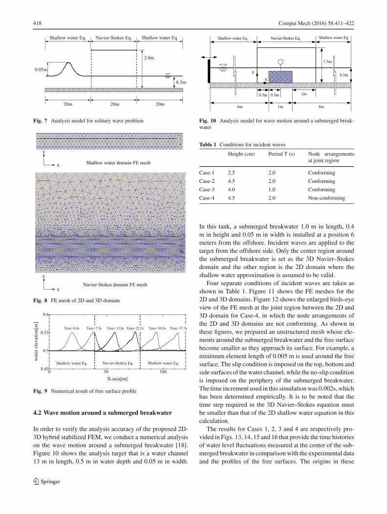
In order to demonstrate the validity of the presentmethod, weconducted a numerical analysis of the solitary wave problem.Figure 7 shows the analysis model that is a water channel 120m in length, 0.5 m in water depth and 0.05 m in width. Theinitial condition of the solitary wave is set at 0.05 m high.The center region is set as the 3D Navier–Stokes domain andthe other regions are the 2D shallow water domains. Figure 8shows the FE meshes for the 2D and 3D domains. The slipcondition is imposed on the top, bottom and side surfaces ofthe water channel. The time increment was set at be 0.01s.Figure 9 shows the obtained free surface profiles at differenttime steps. It can be seen from the result that the wave passedthough the interface between the 3D and the 2D domainswithout any discrepancy.

123

418 Comput Mech (2016) 58:411–422

Fig. 7 Analysis model for solitary wave problem

Fig. 8 FE mesh of 2D and 3D domain

Fig. 9 Numerical result of free surface profile

4.2 Wave motion around a submerged breakwater

In order to verify the analysis accuracy of the proposed 2D-3D hybrid stabilized FEM, we conduct a numerical analysison the wave motion around a submerged breakwater [18].Figure 10 shows the analysis target that is a water channel13 m in length, 0.5 m in water depth and 0.05 m in width.

Fig. 10 Analysis model for wave motion around a submerged break-water

Table 1 Conditions for incident waves

Height (cm) Period T (s) Node arrangementsat joint region

Case-1 2.5 2.0 Conforming

Case-2 4.5 2.0 Conforming

Case-3 4.0 1.0 Conforming

Case-4 4.5 2.0 Non-conforming

In this tank, a submerged breakwater 1.0 m in length, 0.4m in height and 0.05 m in width is installed at a position 6meters from the offshore. Incident waves are applied to thetarget from the offshore side. Only the center region aroundthe submerged breakwater is set as the 3D Navier–Stokesdomain and the other region is the 2D domain where theshallow water approximation is assumed to be valid.

Four separate conditions of incident waves are taken asshown in Table 1. Figure 11 shows the FE meshes for the2D and 3D domains. Figure 12 shows the enlarged birds-eyeview of the FE mesh at the joint region between the 2D and3D domain for Case-4, in which the node arrangements ofthe 2D and 3D domains are not conforming. As shown inthese figures, we prepared an unstructured mesh whose ele-ments around the submerged breakwater and the free surfacebecome smaller as they approach its surface. For example, aminimum element length of 0.005 m is used around the freesurface. The slip condition is imposed on the top, bottom andside surfaces of thewater channel, while the no-slip conditionis imposed on the periphery of the submerged breakwater.The time increment used in this simulationwas 0.002s,whichhas been determined empirically. It is to be noted that thetime step required in the 3D Navier–Stokes equation mustbe smaller than that of the 2D shallow water equation in thiscalculation.

The results for Cases 1, 2, 3 and 4 are respectively pro-vided in Figs. 13, 14, 15 and 16 that provide the time historiesof water level fluctuations measured at the center of the sub-merged breakwater in comparisonwith the experimental dataand the profiles of the free surfaces. The origins in these

123

Comput Mech (2016) 58:411–422 419

Fig. 11 FE mesh of 2D and 3D domain

Fig. 12 Enlarged birds-eye view of the FEmesh at the joint region (forCase-4)

figures are the times when the steady states are realized,respectively. As can be seen from these figures, the numeri-cal results are in agreement with the experimental ones. Also,no disturbance is observed in the profiles of the water sur-faces around both the submerged breakwater and the jointdomain of the 2D–3D domains, demonstrating the stabilityof the proposed numerical method thanks to the performanceof the stabilized FEM.

In order to confirm the capabilities of the MPC and trans-mission methods introduced in the previous section, let usfocus our eyes on Cases-4, where the node arrangement does

Fig. 13 Numerical result: Case-1

Fig. 14 Numerical result: Case-2

not conform at the 2D–3D joint, and Case-2, in which thesame incident wave is used. The result of Case-4 is com-pared with that of Case-2 in Fig. 16, in which the two waveprofiles overlap. It can be confirmed from this comparison

123

420 Comput Mech (2016) 58:411–422

Fig. 15 Numerical result: Case-3

Fig. 16 Numerical result: Case-4 along with the result of Case-2

that the MPC and transmission methods implemented intothe proposed 2D–3D hybrid method function properly.

In order to examine whether or not the 3D effects at theinterfaces between the 2D and 3D domains are negligible in

Fig. 17 Numerical result: Case3 and Case3-w

the above numerical example, we have conducted an addi-tional numerical simulation, of which 3D analysis domainis twice as large as the original setting in the X-direction.The interfaces of this doubled size of the 3D Navier–Stokesdomain with the 2D domains are supposed to have the 3Deffects at less than the original ones. We call this additionalcase Case-3-w and employ the same analysis condition as inCase-3, which achieves the most severe condition in termsof the Froude number. Figure 17 shows the time histories ofwater level fluctuations on the free surface measured directlyabove the center of the submerged breakwater in comparisonwith those of Case-3 and the experiment. As can be seen fromthis figure, the profiles of Case-3-w andCase-3 are almost thesame and in agreement with the experimental result. There-fore, it seems to be safe to conclude that that the 3D effectsaround the interfaces are negligibly small, as the interface isset far enough away from the region where the 3D effects areconsiderable.

The final remark is made about the superiority in terms ofthe computational cost. If we generated the 3D mesh of allthe analysis domain with the same fineness as that around thesubmerged breakwater, including 2D domain in this analysis,the number of DOF would become larger. This provisionalcalculation demonstrates that the proposed method enablesus to simulate the offshore wave propagation and tsunamirunup on a regional scale at relatively low computationalcost.

123

Comput Mech (2016) 58:411–422 421

Fig. 18 Analysis model for tsunami runup problem in an area involv-ing some structures

4.3 Analysis of tsunami runup with structures

As a preliminary examination for the applicability of theproposed method to actual problems we simulate a tsunamirunup involving some structures in a virtual urban area asshown in Fig. 18. Here, the offshore region 400 m in lengthis set for the 2D shallowwater equation,while the 3DNavier–Stokes equation is solved in the remaining region with asubmerged breakwater and onshore structures.

A water column with the width of 80 m and the waterlevel of 10 m is initially located about 300 meters off thecoast and is broken to generate an artificial tsunami wave.The slip condition is imposed on the top, bottom and sidesurfaces and the periphery of the breakwater, while the no-slip condition is imposed on the peripheries of the submergedbreakwater and buildings. A 3D unstructured mesh is gen-erated with a minimum element length of about 0.5 m inthe runup area that ranges from the submerged breakwaterto the region involving the buildings. Figure 19 shows theFE mesh around the onshore structures. The analysis withno submerged breakwater is also carried out for the sake ofcomparison.

Figures 20 and 21 respectively show the runup analysisresults of the cases with and without the submerged break-water. It can be seen from these results that the wave forthe former case spends more time than that of the latter toreach the runup area. It is thus safe to conclude that the pro-posed method can be successfully capture the effect of thesubmerged breakwater on the delay in the arrival time of thetsunami runup.Also, since the unstructuredmeshes conform-

Fig. 19 Mesh around onshore structures

Fig. 20 Numerical result of tsunami runup analysis with submergedbreakwater

Fig. 21 Numerical result of tsunami runup analysiswithout submergedbreakwater

123

422 Comput Mech (2016) 58:411–422

ing to the surface configurations of the onshore structuresare used, the flow regimes around the them are very sta-ble. Based on these results, it is confirmed that the proposedmethod is effective in simulating offshore wave propagationand tsunami runup on a regional scale involving 3D charac-teristics.

5 Conclusions

This study proposes a 2D–3D hybrid stabilized FEM to sim-ulate the offshore wave propagation and tsunami runup on aregional scale with high accuracy and at low computationalcosts. The 2D shallow water equation is employed for theoffshore wave propagation and the 3D Navier–Stokes equa-tion is employed for the runup. The VOF method is appliedto capture free-surface flows in the 3D region. To satisfythe continuity conditions for flow velocities and pressures,the standard MPCmethod is adopted. Also, the transmissionmethod is introduced to approximate the vertical componentof the flow velocity on the boundary of the 3DNavier–Stokesdomain located next to the 2D shallowwater domain. Thanksto theMPC function, the continuity conditions of flow veloc-ities and pressures at the interface can be satisfied even whenunstructuredmeshes, whichmight not conform to each other,are independently generated for 2D and 3D domains.

In the numerical examples, we dealt with the problem ofwave propagations around a submerged breakwater to con-firm the accuracy and stability, and the problem of a tsunamirunup involving submerged and onshore structures to demon-strate the capability and effectiveness of the proposed 2D–3Dhybrid method.

Acknowledgments This study is conducted with support from theGrants-in-Aid for Scientific Research (A) (Research Project No.:25246043) “Multi-scaleNumericalExperiments forEvaluationof Inter-action between Runup Tsunami and Structures”. We are grateful for thesupport.

References

1. KashiyamaK, SaitohK,BehrM,TezduyarTE (1997) Parallel finiteelement methods for large-scale computation of storm surges andtidal flows. Int J Numer Methods in Fluids 24:1371–1389

2. Heniche M, Secretan Y, Boudreau P, Leclerc M (2000) A two-dimensional finite element drying-wetting shallow water modelfor rivers and estuaries. Adv Water Resour 23:360–371

3. Bunya S, Kubotko EJ, Westerink JJ, Dawson C (2009) Wettingand drying treatment for the Runge-Kutta discontinuous Galerkinsolution to the shallow water equations. Comput Methods ApplMech Eng 198:1548–1562

4. Takase S, Kashiyama K, Tanaka S, Tezduyar TE (2011) Space-time SUPGfinite element computation of shallow-water flowswithmoving shorelines. Comput Mech 48:293–306

5. Yamazaki Y, Cheung KF, Kowalik Z (2011) Depth-integrated,non-hydrostatic model with grid nesting for tsunami generation,propagation, and run-up. Int J Numer Methods Fluids 67:2081–2107

6. Guan M, Wright NG, Sleigh PA (2013) A robust 2D shallow watermodel for solving flow over complex topography using homoge-nous flux method. Int J Numer Methods Fluids 73:225–249

7. Aliabadi S, Abedi J, Zellars B, Bota K, Johnson A (2003) Simula-tion technique for wave generation. Commun NumerMethods Eng19:349–359

8. MasamuraK, FujimaK,Goto C, LidaK (2000) Numerical analysisof tsunami by using 2D/3D hybrid model. J. JSCE II 54:49–61 (inJapanese)

9. Masamura K, Fujima K, Goto Shigemura T (2001) Examinationsof fluid forces on the structure by using 2D/3D hybrid model. ProcHydraul Eng JSCE 45:1243–1248 (in Japanese)

10. Fujima K, Masamura K, Goto C (2002) Development of the2D/3D hybrid model for tsunami numerical simulation. Coast EngJ 44(4):373–397

11. Pringle W, Yoneyama N (2013) The application of a hybrid 2D/3Dnumerical tsunami inundation-propagation flow model to the 2011off the pacific coast of Tohoku earthquake tsunami. J JSCE Ser B2(Coastal Engineering) 69(2):I_306–I_310 (in Japanese)

12. Liu GR, Quek SS (2003) The finite element method : a practicalcourse. Butterworth-Heinemann, Oxford

13. Brooks AN, Hughes TJR (1982) Streamline-upwind/Petrov-Galerkin formulations for convection dominated flows with par-ticular emphasis on the incompressible Navier-Stokes equations.Comput Methods Appl Mech Eng 32:199–259

14. Tezduyar TE (1991) Stabilized finite element formulations forincompressible flow computations. Adv Appl Mech 28:1–44

15. Aliabadi S, Tezduyar TE (2000) Stabilized-finite-element/interface-caputuring technique for parallel computationof unsteady flows with interfaces. Comput Methods Appl MechEng 190:243–261

16. Bova SW, Carey GF (1996) A symmetric formulation and SUPGscheme for the shallow-water equations. Adv Water Resour19(3):123–131

17. Matsumoto J, Umetsu T, Kawahara M (2003) Stabilized bubblefunction method for shallow water long wave equation. Int J CompFluid Dyn 17:319–325

18. Sakuraba M, Kashiyama K (2003) Free surface flow using levelsetmethod based on stablized finite element method. Proc Coast EngJSCE 50:16–22 (in Japanese)

123