Estimating the Lifetime Distribution Function Fx(t)

In this section we will see how to use observations from an investigation to obtain an empirical estimate of the distribution function F(t) = P[T ≤t].

The simplest method would be to observe a large no. of new born live and follow them throughout their lifetime. The proportion alive at age t>0 would be an estimate of S(t). The estimate would be a step function, and the larger the sample the closer to a smooth sample we would expect it to be.

Note: this is a non-parametric approach to estimating T - it is the empirical distribution of T.

Problems with this approach:Even if a satisfactory group of lives could be found, the experiment would take about 100 years to complete.In practice we would not be able to observe the deaths of all the lives in the sample. Excluding such lives from the analysis would bias the result. This problem is known as censoring. All we know about censored lives is that they died after a certain age.

1

Censoring Mechanisms

Data are censored if we do not know the exact values of each observation but we do have information about the value of each observation relative to one or more bounds.Censoring is a key feature of survival data and has a profound impact on the estimation procedure. Censoring occurs in a number of different forms:

Right CensoringData are right censored if the censoring mechanism cuts short observations in progress. Eg: the ending of a mortality investigation before all the lives being observed have died. Persons still alive when the investigation ends are right censored – we only know that their lifetimes exceed some value.

Start DeathCensored

t = 0 t T > t

2

Left CensoringData are left censored if the censoring mechanism prevents us from knowing when entry into the state that we wish to observe took place. Eg: medical examinations in which patients are subject to regular examinations. Discovery of a condition tells us inly that the onset fell in the period since the previous examination, the time elapsed since onset has been left censored.

Interval CensoringData are censored if the observational plan only allows us to say that an event of interest fell within some interval of time. Eg: an actuarial investigation where we only know the calendar year of death. Both right and left censoring can be seen as special cases of interval censoring.

Fell ill DeathFound ill

t1 t2 t3

Start DeadDeath

t = 0 t t2

Alive

t1

3

Random CensoringIf the censoring is random then the time Ci at which the observation of the ith lifetime is censored is a random variable. The observation will be censored if Ci < Ti where Ti is the (random) lifetime if the i th life. In such a situation censoring is said to be random.Random censoring is a special case of right censoring.

Non-Informative CensoringCensoring is non-informative if it gives no information about the lifetimes {Ti}. If each member of the pair {Ti, Ci} is independent then censoring is non-informative.

Note: if we are dealing with events that are statistically independent the likelihood function representing all the events is simply the product of the likelihood functions for each individual event. This greatly simplifies the mathematics required in the analysis!

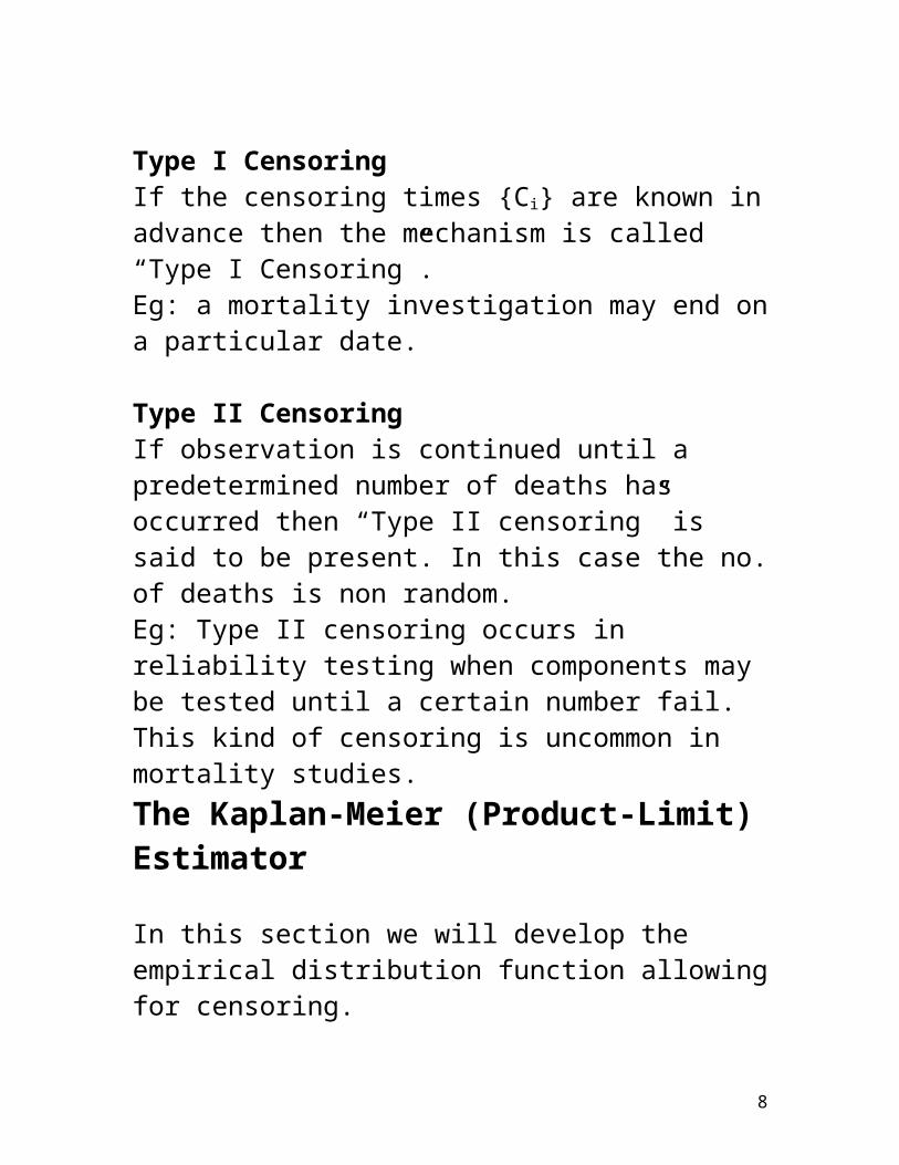
Type I CensoringIf the censoring times {Ci} are known in advance then the mechanism is called “Type I Censoring”.Eg: a mortality investigation may end on a particular date.

Type II CensoringIf observation is continued until a predetermined number of deaths has occurred then “Type II censoring” is said to be present. In this case the no. of deaths is non random.Eg: Type II censoring occurs in reliability testing when components may be tested until a certain number fail. This kind of censoring is uncommon in mortality studies.

4

The Kaplan-Meier (Product-Limit) Estimator

In this section we will develop the empirical distribution function allowing for censoring.

Note: we will consider lifetimes as a function t without mention of a starting age x. The theory can be applied equally to new-born lives, to lives aged x at outset or to lives diagnosed with a medical condition at t = 0.

Assumptions and NotationAssuming non informative censoring consider a population of N lives and suppose we observe m deaths.

Let t1 < t2 < ……< tk be the observed times at which deaths are observed. Note: we do not assume that k = m, so more than one death may be observed at a single failure time.

Suppose that dj deaths are observed at time tj (1<j<k) so that d1 + d2+…+dk = m.

Observation of the remaining N-m lives is censored.

Let cj be the no. of censored lives between times tj and tj+1 (0<j<k). We define t0 = 0 and tk+1 = ∞ to allow for censored observations after the last observed failure time(death) - therfore c0+c1+…+ck = N-m.(In other words cj represents the number of lives that are removed from the investigation between times tj and tj+1 for reasons other than decrement we are investigating.)

5

If cj lives are censored in the interval (tj, tj+1) then the times at which the lives are censored within this interval are tj1, tj2,… .

Finally we define nj to be the number of lives who are alive and at risk at time , that is, just before the j th death time (1 <j<k).

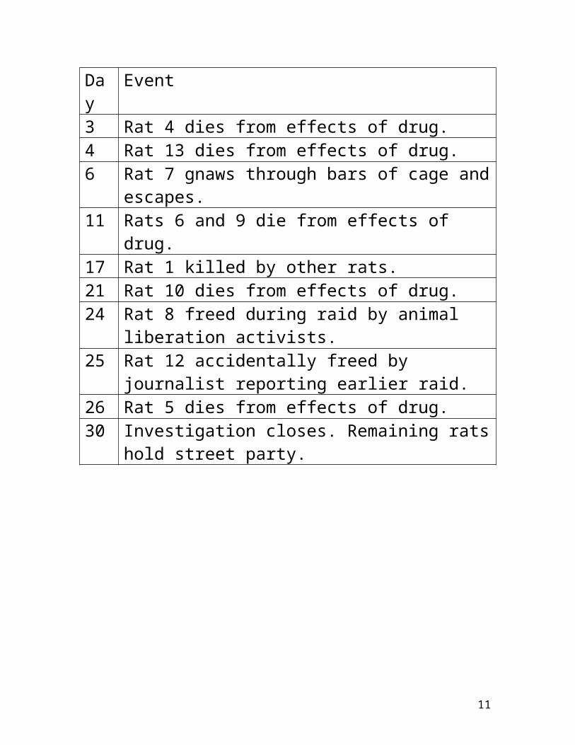
Example A group of 15 laboratory rats are injected with a new drug. They are observed over the next 30 days.

The following events occur:Day Event3 Rat 4 dies from effects of drug.4 Rat 13 dies from effects of drug.6 Rat 7 gnaws through bars of cage and escapes.11 Rats 6 and 9 die from effects of drug.17 Rat 1 killed by other rats.21 Rat 10 dies from effects of drug.24 Rat 8 freed during raid by animal liberation activists.25 Rat 12 accidentally freed by journalist reporting

earlier raid.26 Rat 5 dies from effects of drug.30 Investigation closes. Remaining rats hold street party.

6

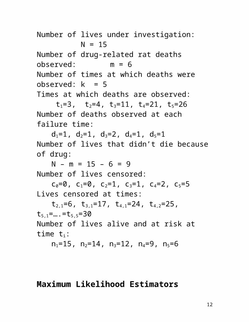
Number of lives under investigation: N = 15Number of drug-related rat deaths observed: m = 6Number of times at which deaths were observed: k = 5Times at which deaths are observed:

t1=3, t2=4, t3=11, t4=21, t5=26Number of deaths observed at each failure time:

d1=1, d2=1, d3=2, d4=1, d5=1Number of lives that didn’t die because of drug:

N – m = 15 – 6 = 9Number of lives censored:

c0=0, c1=0, c2=1, c3=1, c4=2, c5=5Lives censored at times:

t2,1=6, t3,1=17, t4,1=24, t4,2=25, t5,1=….=t5,5=30Number of lives alive and at risk at time ti:

n1=15, n2=14, n3=12, n4=9, n5=6

Maximum Likelihood Estimators

We want to obtain the likelihood of these observations without making any prior assumptions about the form of F(t).

DeathsThe probability of that a death occurs at time tj is .

7

Censored ObservationsThe probability that a life should survive to be censored at time tjl is 1-F(tjl) (assuming non informative censoring).As observed deaths and censored observations are assumed to be independent the total likelihood is:

This can be rewritten as:

The function that maximises this likelihood will be the maximum likelihood estimator of the distribution function.

The factor (1-F(tjl)) is maximised if:1.) F(tjl) = F(tj)

Remember that the distribution function is non-decreasing and that tjl lies in the interval (tj, tj+1). Therefore in order to maximise (1-F(tjl)) = P(T > tjl) we have to minimise F(tjl) = P(T≤tjl). This will be when F(tjl) = F(tj).

2.) F(tj) > F( ) or the likelihood will be zeroTherefore any maximum likelihood estimate of F(t) will be a step function with jumps at each observed lifetime.

Extending the Force of Mortality to Discrete Distributions

8

Suppose F(t) has probability masses at the points t1, t2,…tk. Then:

λj = P[T = tj | T ≥ tj] (1 ≤ j ≤ k)This is called the discrete hazard function.

The Kaplan-Meier Estimate

With the convention that F(0) = 0, d0 = 0, t0=0, tk+1 = ∞ the likelihood can be written:

The first term is the likelihood of observing dj deaths at time tj given that dj lives survived to time .The second term represents the likelihood of :

the dj lives that died at time tj having survived to time and

all censored lives having survived until the times at which the observations were censored (tjl).

As F(t) is a step function that is constant over the interval (tj, tj+1) it follows that: 1-F(tjl) = P(T>tjl)=P(T>tj)=1-F(tj)

Therefore we can write the likelihood as:

This is equivalent to:

9

By definition the first term is just:

Now since we have assumed that T has a discrete distribution and that the only possible value of T are t1,t2,…tk, we can write:

P(T>tj)=P(T≥tj+1) for j=0,1,….kP(T≥t0)=P(T≥t1)=1

So the second term in the likelihood is equal to:

Also, since: for j=1,2,…k

we can write:

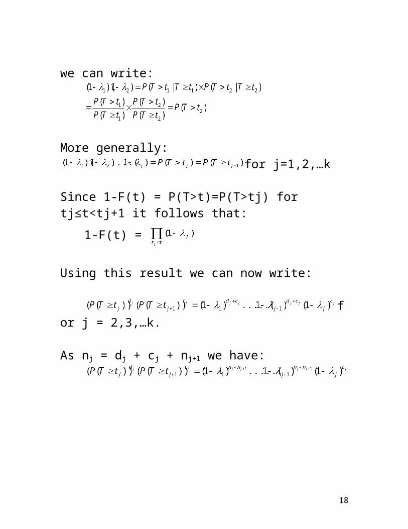
More generally:for j=1,2,…k

Since 1-F(t) = P(T>t)=P(T>tj) for tj≤t<tj+1 it follows that:

10

1-F(t) =

Using this result we can now write:

for j = 2,3,…k.

As nj = dj + cj + nj+1 we have:

11

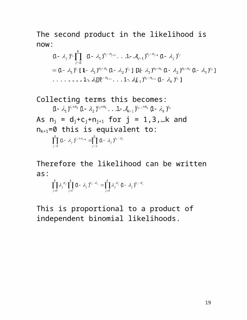
The second product in the likelihood is now:

Collecting terms this becomes:

As nj = dj+cj+nj+1 for j = 1,3,…k and nk+1=0 this is equivalent to:

Therefore the likelihood can be written as:

This is proportional to a product of independent binomial likelihoods.

12

Therefore the maximum likelihood estimator is:

(1 ≤ j ≤ k)

(Proof – on board)

In other words we estimate the discrete hazard function, λj, by dividing the number of deaths observed at time tj by the number of lives at risk at time (1≤j≤k). This is a very intuitive result.

Therefore the Kaplan-Meier (or Product-Limit) estimate of the distribution function of T is:

13

ExampleUsing the data from the observation of laboratory rats, calculate the Kaplan-Meier estimate of F(t).

Solutionj tj dj nj

1 3 1 15 0.06667 0.93333 0.06667

2 4 1 14 0.07143 0.92857 0.13333

3 11 2 12 0.16667 0.83333 0.27778

4 21 1 9 0.11111 0.88889 0.35803

5 26 1 6 0.16667 0.83333 0.46503

Therefore:

14

In calculating the Kaplan-Meier estimate we can divide the time-axis to:

have very short time intervals containing each tj and longer time intervals containing only censored observations.

or alternatively we can choose finer and finer partitions of the time axis and estimate(1-F(t)) as the product of the probabilities of surviving each sub-interval.

Only those at risk of the observed lifetimes {tj} contribute to the estimate therefore it is unnecessary to start observation on all lives at the same time or age – the estimate is valid for data truncated from the left provided the truncation is non-informative.

15

Comparing Lifetime Distributions

Since the Kaplan-Meier estimates are often used to compare the lifetime distributions of two or more populations their statistical properties are important.Greenwood’s formulae approximates the variance of :

and is reasonable over most t but might tend to understate the variance in the tails of the distribution.

Now that we have a measure of the approximate variance of our maximum likelihood estimate of F(t) we can calculate confidence intervals at given value of t.

16

The Nelson-Aalen Estimate

The Nelson-Aalen estimator is another non parametric approach to calculating the empirical distribution function

which is also based on the assumption of non-informative censoring.

The Nelson-Aalen estimate estimates the integrated hazard:

Where the integral deals with the continuous part of the distribution and the sum with the discrete part.

As λj is the proportion of people dying at exact age tj we

can estimate λj using .

In real life hazards (such as death) that we theorise to be operating continuously can only occur discretely. So the continuous part disappears and we are left with

as our estimate of the integrated hazard function.

17

The Nelson-Aalen estimate of the survival function is therefore:

and the distribution function is:

Corresponding to Greenwoods formula the formula for the variance of the Nelson-Aalen estimator is:

18

Relationship between the Kaplan-Meier and Nelson-Aalen Estimates

The Kaplan-Meier estimate can be approximated in terms of .

Where s is the number of times that deaths have occurred before exact time t.

Using the approximation ex ≈ 1+x for small x we have:

ExampleThe following data relate to 12 patients who had an operation – time 0 is the start of the investigation.

Patient

No.

Time of Operation(in weeks)

Time observation ended (in weeks)

Reason observation ended

19

1 0 120 Censored2 0 68 Death3 0 40 Death4 4 120 Censored5 5 35 Censored6 10 40 Death7 20 120 Censored8 44 115 Death9 50 90 Death10 63 98 Death11 70 120 Death12 80 110 DeathYou can assume that the censoring was non informative with regard to the survival of any individual patient.

(i) Compute the Nelson-Aalen estimate of the cumulative hazard function, Λ(t), where t is the time since having the operation.

(ii) Using the result of part (i) deduce an estimate of the survival function for patients who have had this operation.

(iii) Estimate the probability of a patient surviving for at least 70 weeks after undergoing the operation.

20