arX

iv:1

409.

0287

v1 [

astr

o-ph

.CO

] 1

Sep

201

4

Mon. Not. R. Astron. Soc.000, 1–12 () Printed 2 September 2014 (MN LATEX style file v2.2)

2MTF IV. A bulk flow measurement of the local Universe

Tao Hong1,2,3⋆, Christopher M. Springob2,3,4, Lister Staveley-Smith2,3,Morag I. Scrimgeour5,6,2,3, Karen L. Masters7,8, Lucas M. Macri9,Barbel S. Koribalski10, D. Heath Jones11, and Tom H. Jarrett121National Astronomical Observatories, Chinese Academy of Sciences, 20A Datun Road, Chaoyang District, Beijing 100012, China.2International Centre for Radio Astronomy Research, M468, University of Western Australia, Crawley, 35 Stirling Highway, WA 6009, Australia3ARC Centre of Excellence for All-sky Astrophysics (CAASTRO)4 Australian Astronomical Observatory, PO Box 915, North Ryde, NSW 1670, Australia5 Department of Physics and Astronomy, University of Waterloo, Waterloo, ON, N2L 3G1, Canada6 Perimeter Institute for Theoretical Physics, 31 Caroline St. N., Waterloo, ON, N2L 2Y5, Canada7Institute for Cosmology and Gravitation, University of Portsmouth, Dennis Sciama Building, Burnaby Road, PortsmouthPO1 3FX8South East Physics Network (www.sepnet.ac.uk)9George P. and Cynthia Woods Mitchell Institute for Fundamental Physics and Astronomy, Department of Physics and Astronomy, Texas A&M University,4242 TAMU, College Station, TX 77843, USA10CSIRO Astronomy & Space Science, Australia Telescope National Facility, PO Box 76, Epping, NSW 1710, Australia11School of Physics, Monash University, Clayton, VIC 3800, Australia12Astronomy Department, University of Cape Town, Private BagX3. Rondebosch 7701, Republic of South Africa

Accepted ... Received ...

ABSTRACTUsing the 2MASS near-infrared photometry and high signal-to-noise HI 21-cm data from theArecibo, Green Bank, Nancay, and Parkes telescopes, we calculate the redshift-independentdistances and peculiar velocities of 2,018 bright inclinedspiral galaxies over the whole sky.This project is part of the 2MASS Tully-Fisher survey (2MTF), aiming to map the galaxypeculiar velocity field within 100h−1Mpc, with an all-sky coverage apart from Galactic lat-itudes|b| < 5. A χ2 minimization method was adopted to analyze the Tully-Fisher peculiarvelocity field in J, H and K bands, using a Gaussian filter. We combine information from thethree wavebands, to provide bulk flow measurements of310.9± 33.9 km s−1, 280.8± 25.0km s−1, and292.3 ± 27.8 km s−1 at depths of 20h−1Mpc, 30 h−1Mpc and 40h−1Mpc,respectively. Each of these bulk flow vectors points in a direction similar to those found byprevious measurements. At each of the three depths, the bulkflow magnitude is consistentwith predictions made by theΛCDM model at the1σ level. The maximum likelihood andminimum variance method were also used to analyze the 2MTF samples, giving similar re-sults.

Key words: galaxies: distances and redshifts — galaxies: spiral — radio emission lines —catalogs — surveys

1 INTRODUCTION

Galaxy redshifts exhibit deviations from Hubble’s law known as‘peculiar velocities’, which are induced by the gravitational attrac-tion of all surrounding matter. Peculiar velocities thus provide ameans to trace the overall matter density field and detect allgravi-tating matter (both visible and dark).

Peculiar velocities can be measured using redshift-independent distance indicators. Several such indicatorshavebeen used, including Type Ia SNe (Phillips 1993), the Tully-Fisherrelation (TF, Tully & Fisher 1977) and the Fundamental Plane

⋆ E-mail: bartonhongtao@gmail.com

relation (FP, Djorgovski & Davis 1987; Dressler et al. 1987). Thelargest peculiar velocity surveys make use of either the FP orTF relations. One limitation of these, and many other, redshiftindependent distance indicators, however, is that they rely onoptical photometry or spectroscopy. This means that the opticalextinction effects of our Galaxy limit the sky coverage of suchsurveys in the so-called Zone of Avoidance (ZoA).

The 2MASS Tully-Fisher Survey (2MTF, Masters et al. 2008;Hong et al. 2013; Masters et al. 2014) is an all-sky Tully-Fishersurvey aiming to measure the redshift-independent distances ofnearby bright spiral galaxies. All galaxies in the 2MTF sample wereselected from the 2MASS Redshift Survey (2MRS, Huchra et al.2012), which is an extended redshift survey based on the 2 Mi-

2 T. Hong et al.

Figure 1. Sky coverage of the 2,018 2MTF galaxies, in Galactic coordinates with an Aitoff projection.

cron All-Sky Survey Extended Source Catalog (2MASS XSC,Jarrett et al. 2000). By using the near-infrared photometric data andhigh quality 21-cm HI data from the Green Bank Telescope (GBT),Parkes radio telescope, Arecibo telescope, and other archival H I

catalogs, 2MTF provides sky coverage down to Galactic latitude|b| = 5, which significantly reduces the area of the ZoA relativeto previous Tully-Fisher surveys.

One parameter of the peculiar velocity field that benefits fromthe improved sky coverage of 2MTF is the dipole, or ‘bulk flow’.In past measurements of the bulk flow of the local universe, au-thors have largely agreed on the direction of the flow, but dis-agree on its amplitude (Hudson et al. 2004; Feldman et al. 2010;Dai et al. 2011; Ma et al. 2012; Ma & Scott 2013; Rathaus et al.2013; Ma & Pan 2014). Watkins et al. (2009) analyzed a peculiarvelocity sample of 4,481 galaxies with a “Minimum Variance”method, within a Gaussian window of radius 50h−1Mpc. Theyfound a bulk flow with amplitude407 ± 81 km s−1, which theyclaim is inconsistent with theΛCDM model at>98% confidencelevel.

On the other hand, other studies have shown a bulk flowamplitude agreeing with theΛCDM model. By estimating thebulk flow of the SFI++ Tully-Fisher sample (Masters et al. 2006;Springob et al. 2007), Nusser & Davis (2011) derived a bulk flowof 333 ± 38 km s−1 at a depth of 40h−1Mpc, which is consis-tent with theΛCDM model. Turnbull et al. (2012) adopted the bulkflow estimation on a Type Ia SNe sample with 245 peculiar velocitymeasurements, finding a bulk flow of249 ± 76 km s−1, which isalso consistent with the expectation fromΛCDM.

In this paper, we use 2MTF data to measure the bulk flow inthe local Universe. The relatively even sky coverage and uniformsource selection criteria make 2MTF a good sample for bulk flowanalysis. The data collection is described in Section 2. Section 3introduces the calculations of Tully-Fisher distances andpeculiarvelocities. Aχ2 minimization method was adopted to analyze thepeculiar velocity field, which is presented in Section 4. We com-pared our measurements with theΛCDM predictions and previousmeasurements in Section 5. A summary is provided in Section 6.

Throughout this paper, we adopt a spatially flat cosmol-ogy with Ωm = 0.27, ΩΛ = 0.73, ns = 0.96 (WMAP-7yr,

Larson et al. 2011). All distances in this paper are calculated andpublished in units ofh−1Mpc, where the Hubble constant is givenby H0 = 100h km s−1 Mpc−1. The observational results in thispaper are independent of the actual value ofh, though we comparewith aΛCDM model in Section 5 which assumes the WMAP-7yrvalue ofh = 0.71.

2 DATASETS

To build a high quality peculiar velocity sample, all 2MTF targetgalaxies are selected from 2MRS using the following criteria: totalK magnitudes K< 11.25 mag,cz < 10, 000 km s−1, and axis ra-tio b/a < 0.5. There are∼ 6, 000 galaxies that meet these criteria,but many of them are faint in HI, so observing the entire samplewould be very expensive in terms of telescope time. We have com-bined archival HI data with observations from the Arecibo LegacyFast ALFA survey (ALFALFA, Giovanelli et al. 2005) and new ob-servations made with the GBT and Parkes radio telescope. Thenewobservations preferentially targeted late-type spirals deemed likelyto be HI rich, but the archival data includes all spiral subclasses.Accounting for galaxies eliminated from the sample becauseofconfusion, marginal SNR, non-detections, and other problematiccases, as well as cluster galaxies reserved for use in the 2MTF tem-plate (Masters et al. 2008), current peculiar velocity sample from2MTF catalog contains 2,018 galaxies. As shown in Figure 1, thecatalog provides uniform sky coverage down to Galactic latitude|b| = 5, which makes it a good sample for bulk flow and large-scale structure analysis.

We note that the sample of 2,018 galaxies discussed here isseparatefrom the 888 cluster galaxies used to fit the template re-lation for 2MTF in Masters et al. (2008). The relationship betweenthat template sample and the field sample is discussed further inSection 3.1.

2.1 Photometric Data

All 2MTF photometric data are obtained from the 2MRS cat-alog. 2MRS is an all-sky redshift survey based on 2MASS. It

2MTF IV. Bulk flow 3

0.1

0.2

0.3

0.4

0.5

0.6

0.7

0.8

0.9

1

0.1 0.2 0.3 0.4 0.5 0.6 0.7 0.8 0.9 1

2M

AS

S c

o-a

dd

ed a

xis

-rat

io

Axis-ratio used in Masters et al. 2008

Figure 2. The comparison between the axis-ratios adopted by Masters et al.(2008) and the 2MASS co-added axis-ratios. The solid line indicates equal-ity. 888 template galaxies used by Masters et al. (2008) are plotted here.The scatter of these two axis-ratios is 0.096.

provides more than 43,000 redshifts of 2MASS galaxies, withK< 11.75 mag and|b| > 5. The photometric quantities whichare adopted for the Tully-Fisher calculations are the totalmagni-tudes in J, H and K bands, the 2MASS co-added axis-ratiob/a (theaxis-ratio of J+H+K image at the 3σ isophote; for more details seeJarrett et al. 2000) and the morphological type codeT .

Masters et al. (2008) built the 2MTF Tully-Fisher template us-ing the axis-ratio in I-band and J-band. However, the I-bandaxis-ratios are only available for a small fraction of the 2MTF non-template galaxies. Thus, to make the 2MTF non-template samplemore uniform, we chose the 2MASS co-added axis-ratio as our pre-ferred data. As shown in Figure 2, we took the 888 2MTF templategalaxies as a comparison sample and compared the 2MASS co-added axis-ratios with the axis-ratios used in the 2MTF template.A dispersion was found between these two parameters (∼ 0.096),which we expect will introduce a small scatter into the final Tully-Fisher relation, but no significant bias was detected in thiscompar-ison.

Galaxy internal dust extinction andk-correction were donefollowing Masters et al. (2008). The total magnitudes provided bythe 2MRS catalog have already been corrected for Galactic extinc-tion, so no additional such correction was applied here.

2.2 H I Rotation Widths

2.2.1 Archival Data

Before making our new HI observations, we collected high-quality H I width measurements from the literature. The primarysource of 2MTF archival data is the Cornell HI digital archive(Springob et al. 2005). The Cornell HI digital archive providesabout 9,000 HI measurements in the local Universe (−200 <cz < 28, 000 km s−1) observed by single-dish radio telescopes.When cross-matching this HI dataset with the 2MRS catalog, weinclude only the galaxies with quality codes suggesting suitabilityof the measured width for TF studies, G (Good) and F (Fair) in the

nomenclature of Springob et al. (2005). (See Section 4 of that pa-per for details.) 1,038 well-measured galaxies in this dataset whichmeet the 2MTF selection criteria were taken into the final 2MTFcatalog. The HI widths provided by Springob et al. (2005) werecorrected for redshift stretch, instrumental effects and smoothing,we have added the turbulence correction and viewing angle cor-rection to make the corrected widths suitable for the Tully-Fishercalculations.

Besides the Cornell HI digital archive, we also collected HIdata from Theureau et al. (1998, 2005, 2007); Mathewson et al.(1992) and Nancay observed galaxies in Table A.1 of Paturel et al.(2003). The raw observed widths taken from these sources werecorrected for the aforementioned observational effects followingHong et al. (2013).

2.2.2 GBT and Parkes Observations

In addition to the archival HI data, new observations were con-ducted by the Green Bank Telescope (GBT) and the Parkes radiotelescope between 2006 to 2012.

1,193 2MTF target galaxies in the region ofδ > −40 wereobserved by the GBT (Masters et al. 2014) in position-switchedmode, with the spectrometer set at 9 level sampling with 8192channels. After smoothing, the final velocity resolution was 5.15km s−1. The HI line was detected in 727 galaxies, with 483 ofthem considered good enough to be included into the 2MTF cata-log.

The Parkes radio telescope was used to observe the targets inthe declination rangeδ 6 −40 (Hong et al. 2013). We observed305 galaxies which did not already have high quality HI measure-ments in the literature and obtained 152 well detected HI widths(signal-to-noise ratio SNR> 5). Beam-switching mode with 7high-efficiency central beams was used in the Parkes observations.The multibeam correlator produced raw spectra with a velocity res-olution∆v ∼ 1.6 km s−1, while we measured HI widths and otherparameters on the Hanning-smoothed spectra with a velocityreso-lution of ∼ 3.3 km s−1.

All newly-observed spectra from the GBT and Parkes tele-scope were measured by the same IDL routineawv fit.pro, whichbased on the algorithm used by Springob et al. (2005). HI linewidths were measured by five different methods (see Hong et al.2013, Section 2.1.2). We choseWF50 as our preferred width al-gorithm. This fitting method can provide accurate width measure-ments for low S/N spectra. It was adopted as the preferred methodby the Cornell HI digital archive and the ALFALFA blind HI sur-vey.

2.2.3 ALFALFA Data

The GBT observations did not cover the entirety of the sky north ofδ = −40. 7,000 deg2 of the northern (high Galactic latitude) skywere observed by the ALFALFA survey. In this region of the sky,we rely on the ALFALFA observations, rather than making our ownGBT observations. In this region, ALFALFA is expected to detectmore than 30,000 HI sources with HI mass between106 M⊙ and1010.8 M⊙ out to z∼ 0.06. The ALFALFA dataset has not beenfully released yet. Haynes et al. (2011) published theα.40 catalogwhich covers about40% of the final ALFALFA sky. However, theALFALFA team has provided us with an updated catalog of HI

widths, current as of October 2013. The new catalog covers about66% of the ALFALFA sky. From this database, the 2MTF catalog

4 T. Hong et al.

0

20

40

60

80

100

120

0 1000 2000 3000 4000 5000 6000 7000 8000 9000 10000

Co

un

t

cz [km s-1

]

Figure 3. The redshift distribution of the 2MTF sample in the CMB frame.

obtained 576 HI widths. When the final ALFALFA catalog is re-leased, we will correspondingly update the 2MTF catalog, makinguse of the complete dataset.

2.3 Data collecting limit of Tully-Fisher sample

The initial 2MTF catalog includes 2,708 galaxies. An additionalcutoff was employed to improve the data quality. Only the well-measured galaxies were included in the 2MTF peculiar velocitysample. That is, we include those galaxies withcz > 600 km s−1,relative HI width errorǫw/wHI 6 10% and HI spectrum signal-to-noise ratio SNR> 5. 141 galaxies in the template sample ofMasters et al. (2008) were excluded. The current 2MTF peculiarvelocity sample has 2,018 galaxies with good enough data qualityfor the Tully-Fisher distance calculations and further cosmologicalanalysis. The sky coverage and redshift distribution of the2MTFpeculiar velocity sample are plotted in Figure 1 and Figure 3re-spectively.

3 DERIVATION OF TULLY-FISHER DISTANCES ANDPECULIAR VELOCITIES

3.1 Template Relation

Using 888 spiral galaxies in 31 nearby clusters, Masters et al.(2008) built Tully-Fisher template relations in the 2MASS J, Hand K bands, following the approach taken by Masters et al. (2006)for SFI++, which in turn follows the approach of Giovanelli et al.(1997) for SCI. The authors found a dependence of the TF relationon galaxy morphology, with later spirals presenting a steeper slopeand a dimmer zero point on the relation than earlier type spirals.This morphological dependence occurs in all three 2MASS wave-bands. The final template relations were corrected to the Sc type inthe three bands, as was done for in the I-band relation examined byMasters et al. (2006).

We use the revised version of the Masters et al. (2008) Tully-Fisher relation as our template to calculate the distances of the2MTF galaxies:

MK − 5 log h = −22.188 − 10.74(logW − 2.5),

MH − 5 log h = −21.951 − 10.65(logW − 2.5),

MJ − 5 log h = −21.370 − 10.61(logW − 2.5),

(1)

where W is the corrected HI width in units of km s−1, and

MK ,MH , andMJ are the absolute magnitudes in the three bandsseparately.

3.2 TF distance and peculiar velocity calculations

Since the components of the peculiar velocity uncertainties are log-normal, our bulk flow analysis is done in logarithmic space. Themain parameters used in the fitting processes arelog(dTF) andits corresponding logarithmic error. More precisely, rather than ex-press the peculiar velocity in linear units, we work with thecloselyrelated logarithmic quantitylog(dz/dTF), which is the logarithmof the ratio between the galaxy’s redshift distance in the CMBframe and its Tully-Fisher-derived true distance. At this stage, weexpress this aslog(dz/d∗TF), which represents the logarithmic dis-tance ratio before the Malmquist bias correction has been applied(see Section 3.4.) We can then express this as:

log

(dzd∗TF

)=

−∆M

5, (2)

where∆M = Mobs − M(W ) is the difference between the cor-rected absolute magnitudeMobs (calculated using the redshift dis-tance of the galaxy) and the magnitude generated from the TF tem-plate relationM(W ) (for more details on corrected absolute mag-nitudes, see Equation 7 from Masters et al. 2008).

The errors on the logarithmic distance ratio are the sum inquadrature of the HI width error, near-infrared magnitude error,inclination error, and the intrinsic error of the Tully-Fisher re-lation. Instead of using the intrinsic error estimates reported byMasters et al. (2008), we adopted new intrinsic error terms:

ǫint,K = 0.44 − 0.66(logW − 2.5),

ǫint,H = 0.45 − 0.95(logW − 2.5),

ǫint,J = 0.46 − 0.77(logW − 2.5).

(3)

These relations were derived in magnitude units. To transform theerrors into the logarithmic units used forlog(dz/d∗TF), one mustdivide theǫint values by 5. We describe the details of the new in-trinsic error term estimation in Appendix A.

As shown in Figure 2, the difference between the two sourcesof inclination introduces a mean scatter of 0.096, so we adopted auniform scatterσinc = 0.1 as the inclination error. The inclinationuncertainty then introduces errors into the Tully-Fisher distances.For a galaxy with inclinationb/a, we calculated the corrected HIwidth with b/a ± 0.1, and got the corrected widthsWhigh andWlow respectively. Half of the difference between the two widths,∆wid,inc = 0.5(Whigh −Wlow), was then adopted as the error in-troduced by the inclination into the HI corrected width. Finally, theerror introduced to the Tully-Fisher distances by inclination uncer-tainty, ǫinc, was calculated using the same approach undertaken tocalculate the contribution from the HI width uncertainty,ǫwid.

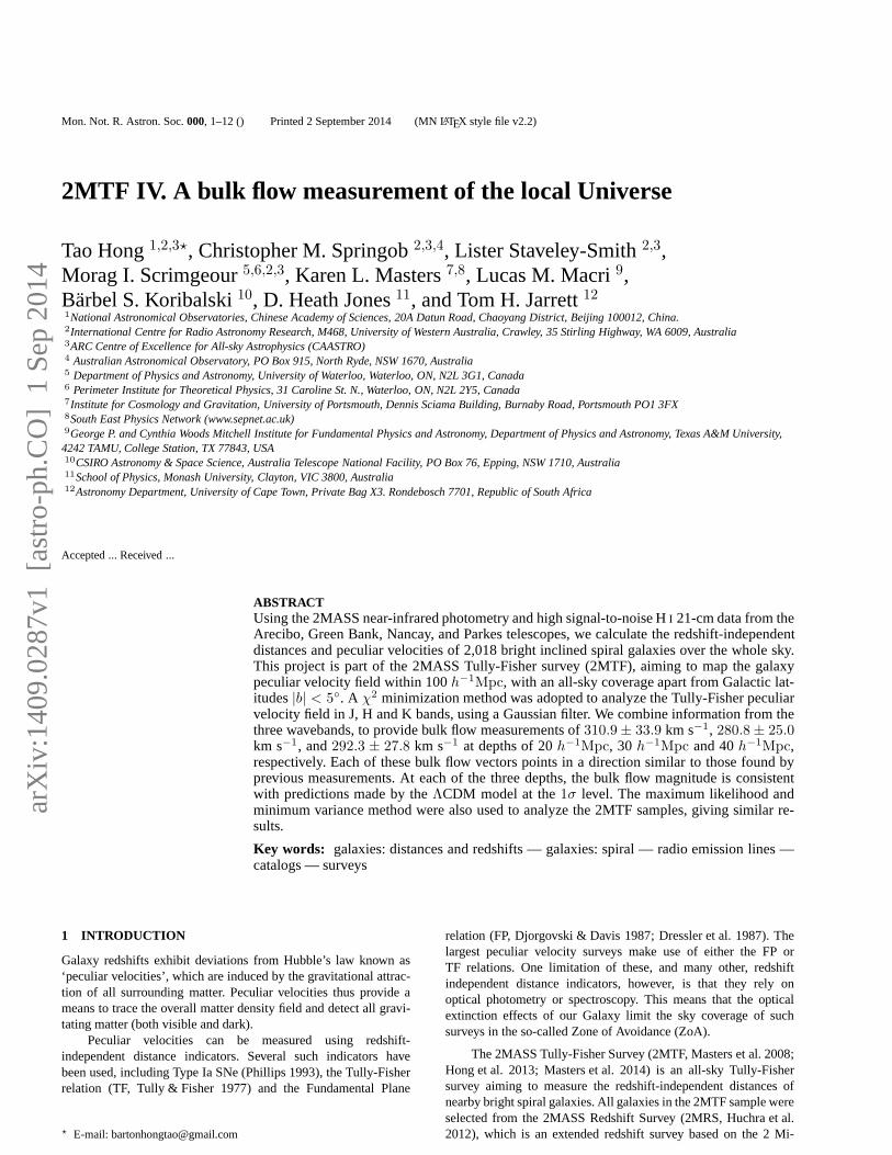
The Tully-Fisher relations in the three bands are shown in Fig-ure 4, along with the template relations. We also show the observa-tional errors for both the HI width and NIR magnitudes.

3.3 Member galaxies of galaxy groups

We cross-matched the 2MTF galaxies with the group list identifiedby Crook et al. (2007). 55 galaxy groups have more than one mem-ber in the 2MTF sample. We assume all member galaxies in a givengroup have the same redshift. That is, when doing the calculation inEquation 2, all member galaxies in a group are assigned the groupredshiftczgroup, while the magnitude offset∆M was still calcu-lated separately for each galaxy.

2MTF IV. Bulk flow 5

-28

-26

-24

-22

-20

-18

-16

-14 1.8 2 2.2 2.4 2.6 2.8 3

MJ

- 5 l

og h

[m

ag]

log (W/km s-1

)

605040302010

-28

-26

-24

-22

-20

-18

-16

-14 1.8 2 2.2 2.4 2.6 2.8 3

MH

- 5

log h

[m

ag]

log (W/km s-1

)

605040302010

-28

-26

-24

-22

-20

-18

-16

-14 1.8 2 2.2 2.4 2.6 2.8 3

MK

- 5

log h

[m

ag]

log (W/km s-1

)

605040302010

Figure 4. Tully-Fisher relations for 2MTF galaxies in the J, H and K bands (left to right). The red solid lines are the TF template relations in the three bands.By making a50 × 50 grid on the Tully-Fisher relation surfacelogW − M , we counted the number of galaxies falling in every grid point, and took thesecounts as the number density of the Tully-Fisher plot, whichare indicated by the color contours.

3.4 Malmquist bias correction

The term ‘Malmquist bias’ describes a set of biases originatingfrom the spatial distribution of objects. There are two types of bi-ases that one may consider. Inhomogeneous Malmquist bias arisesfrom local density variations along the line of sight, and ismuchmore pronounced when one is working in real space. This is be-cause, as explained by Strauss & Willick (1995), the large dis-tance errors cause the observer to measure galaxy distancesscat-tered away from overdense regions in real space. In contrast, themuch smaller redshift errors mean that this effect is insignificantin redshift space. While some other TF catalogs, such as SFI++,included galaxy distances in real space, the fact that we operate inredshift space means that inhomogeneous Malmquist bias is negli-gible. However, we must account for the second type of Malmquistbias, homogeneous Malmquist bias.

Homogeneous Malmquist bias comes about as a consequenceof the selection effects of the survey, which cause galaxiesto bepreferentially included or excluded from the survey, depending ontheir distance. Ideally, the survey selection function is aknown an-alytical function, allowing for a relatively straightforward correc-tion for selection effects. However, galaxy peculiar velocity sur-veys often have complex selection functions, requiring ad hoc ap-proximations in the application of Malmquist bias corrections (e.g.,Springob et al. 2007).

In the case of 2MTF, we used homogeneous criteria in de-termining which galaxies to observe. As explained in Section 2,all 2MRS galaxies with K< 11.25 mag,cz < 10, 000 km/s, andb/a < 0.5 that also met our morphological selection criteria weretargeted for inclusion in the sample. However, many of the targetedgalaxies were not included in the final sample, because therewasno H I detection, the detection was marginal, or there was someother problem with the spectrum that prevented us from making anaccurate Tully-Fisher distance estimate.

We thus adopt the following procedure for correcting forMalmquist bias (explained in more detail by Springob et al. inprep.):

1) Using the stepwise maximum likelihood method(Efstathiou et al. 1988), we derive the K-band luminosityfunction for all galaxies in 2MRS that meet our K-band apparentmagnitude, Galactic latitude, morphological, and axis ratio criteria.For this purpose, we include galaxies beyond the 10,000 km/sredshift limit, to simplify the implementation of the luminosityfunction derivation. For this sample, which we designate the

‘target sample’, we fit a Schechter function (Press & Schechter1974), and findMk∗ = −23.1 andα = −1.10. (The stepwisemaximum likelihood method does not determine the normalizationof the luminosity function, but that is irrelevant for our purposesanyway.) We note that this luminosity function has a steeperfaintend slope than the 2MASS K-band luminosity function derivedbyKochanek et al. (2001), who findα = −0.87.

2) We next assume that the ‘completeness’, which in this casewe take to mean the fraction of the target sample that is includedin our 2MTF peculiar velocity catalog for a given apparent magni-tude bin, is a simple function of apparent magnitude, which is thesame across the sky in a given declination range. We compute thisfunction, simply taking the ratio of observed galaxies to galaxiesin the target sample for K-band apparent magnitude bins of width0.25 mag, separately for two sections of the sky: north and southof δ = −40. This divide in the completeness north and south ofδ = −40 is due to the fact that the GBT’s sky coverage only goesas far south as−40, and the galaxies south of that declinationwere only observed by the somewhat smaller (and therefore lesssensitive) Parkes telescope.

3) Finally, for every galaxy in the 2MTF peculiar velocitysample, we take the uncorrectedlog(dz/d∗TF) value, and the errorǫd, and compute the initial probability distribution oflog(dz/dTF)values, assuming that the errors follow a normal distribution inthese logarithmic units. For each possible value of the loga-rithmic distance ratiolog(dz/dTF,i) within 2σ of the measuredlog(dz/d

∗TF), we weight the probability bywi, where1/wi is the

completeness (as defined in Step 2) integrated across the entireK-band luminosity function (derived in Step 1), evaluated at thelog(dz/dTF,i) in question. Note that this involves converting thecompleteness from a function of apparent magnitude to a functionof absolute magnitude, using the appropriate distance modulus forthe distance in question.

From these newly re-weighted probabilities, we calculatethe mean probability-weighted log(distance), as well as the cor-rected logarithmic distance ratio error. This is our Malmquist bias-corrected logarithmic distance.

The histograms of the logarithmic distance ratioslogdczdTF

with the errors are shown in Figure 5 and Figure 6 respectively.The Tully-Fisher distances plotted here are all Malmquist bias-corrected. A histogram of the relative errors of linear Tully-FisherdistancesdTF is plotted in Figure 7. The mean errors of the Tully-Fisher distances are around22% in all three bands.

6 T. Hong et al.

0

20

40

60

80

100

120

140

160

180

200

-0.4 -0.3 -0.2 -0.1 0 0.1 0.2 0.3 0.4

Co

un

t

log (dcz/dTF)

K-bandH-bandJ-band

Figure 5. The histogram of logarithmic distance ratioslogdcz

dTF

. The K-

band data is shown by the red solid line, H-band data by the green dashedline, and the J-band data by the blue dotted line.

0

50

100

150

200

250

0 0.02 0.04 0.06 0.08 0.1 0.12 0.14 0.16 0.18 0.2

Count

Error of logarithmic distance ratio [dex]

K-bandH-bandJ-band

Figure 6.The histogram of the error of the logarithmic distance ratios, usingthe same color scheme as in Figure 5.

4 BULK FLOW FITTING AND THE RESULTS

4.1 χ2 minimization method

We useχ2 minimization to fit the peculiar velocity field to a simplebulk flow model. As mentioned in Section 3.2, the errors on pecu-liar velocities are log-normally distributed, so we did thefitting inlogarithmic distance space, similarχ2 logarithmic methods wereadopted by Aaronson et al. (1982) and Staveley-Smith & Davies(1989). In the CMB frame, for a bulk flow velocity

−→V , this flow

provides a radial component for each galaxy according to:

vmodel,i =−→V · ri, (4)

whereri is the unit vector pointing to the galaxy. We can also ex-press the model-predicted distance to galaxyi as

dmodel,i =( czi − vmodel,i

100

)h−1Mpc. (5)

In our calculation ofχ2, we apply weights which combinethe measurement errors of the logarithmic distance ratios and theweights generated from both the redshift distribution and the un-even galaxy number density in different sky areas. Ourχ2 value isgiven by:

χ2 =N∑

i=1

[log(dz,i/dmodel,i)− log(dz,i/dTF,i)]2 · wr

iwdi

σ2i ·

∑Ni=1

(wriw

di )

, (6)

0

50

100

150

200

250

10% 15% 20% 25% 30% 35% 40% 45% 50%

Count

Relative error of linear Tully-Fisher distances

K-bandH-bandJ-band

Figure 7. The histogram of the relative errors of linear Tully-Fisherdis-tances, using the same color scheme as in Figure 5.

whereσi is the logarithmic distance ratio error of theith galaxy,wri

is the weight arising from the radial distribution of the sample, andwd

i is the weight weighting for the uneven galaxy number densityin the northern and southern sky.

The weightwri was designed to make the weighted redshift

distribution of the whole sample match the redshift distribution ofan ideal survey. We adopted the Gaussian density profile followingWatkins et al. (2009):

ρ(r) ∝ exp(−r2/2R2I), (7)

with the number distribution

n(r) ∝ r2 exp(−r2/2R2I ), (8)

whereRI indicates the depth of the bulk flow measurement. In thiswork, we adoptRI = 20h−1Mpc, 30h−1Mpc and 40h−1Mpc,in order to show the bulk flow across a range of depths.

Since the 2MTF sample has a denser galaxy distribution in thesky north ofδ = −40, we introduced the weightwd

i to correct theuneven number density in these two sky areas. The regions of thesky north and south of this line contain 1,827 and 191 2MTF galax-ies and subtend 33,885 and 7,368 deg2, respectively. This yields aratio of galaxy number density between the southern and north-ern regions of roughly 1:2.08. We therefore setwd

i = 2.08 for thesouthern objects andwd

i = 1 for the northern ones.To reduce the effect of outliers, we applied two cuts dur-

ing the fitting process. With each successive cut, we did theχ2

minimization first, and compared the difference between thebulkflow-corrected logarithmic distance ratio and the predicted Hub-ble flow logarithmic distance ratio:∆i = log(dz,i/dmodel,i) −log(dz,i/dTF,i). The outliers with∆i > 3σi were then removed.We did the clipping twice, then applied the thirdχ2 minimization,and report the result as the final bulk flow velocity. The totalnum-ber of galaxies removed from the sample is around 60.

The fitting errors were calculated via the jackknife method.We built 50 jackknife subsamples by randomly removing 2% ofthe 2MTF sample, ensuring that each galaxy was removed in onesubsample only. For every jackknife subsample, theχ2 minimiza-tion fitting was adopted, and the error on the bulk flow was takenas:

ǫV =

[N − 1

N

N∑

i=1

(V Ji − V

J)2

]1/2

, (9)

whereN = 50 is the number of jackknife subsamples,V Ji is the

2MTF IV. Bulk flow 7

bulk flow for theith jackknife subsample, andVJ= 1

N

∑Ni=1

V Ji .

The velocity components in three directions (VX , VY , VZ) were es-timated using Equation 9.

To analyze the performance of theχ2 minimization method,we simulated 1,000 mock catalogs and tested the method with thesesimulated data. We built the mock catalogs based on the real 2MTFdata sample, with each catalog containing 2,018 mock galaxies.These galaxies have the same sky position and redshift as thereal2MTF galaxies. In each mock catalog, we set the input bulk flowvelocity equals to the same value as our measurement of the K-banddata sample at the depth ofRI = 30 h−1Mpc, i.e.,VX = 163.4km s−1, VY = −308.3 km s−1 andVZ = 107.7 km s−1. Wesimulated distance errors by using a Gaussian random variable toinduce mock scatter in the TF, with a variance equals to the totallogarithmic distance error for that galaxy. The average value of thislogarithmic distance error is 0.096, as in the real data.

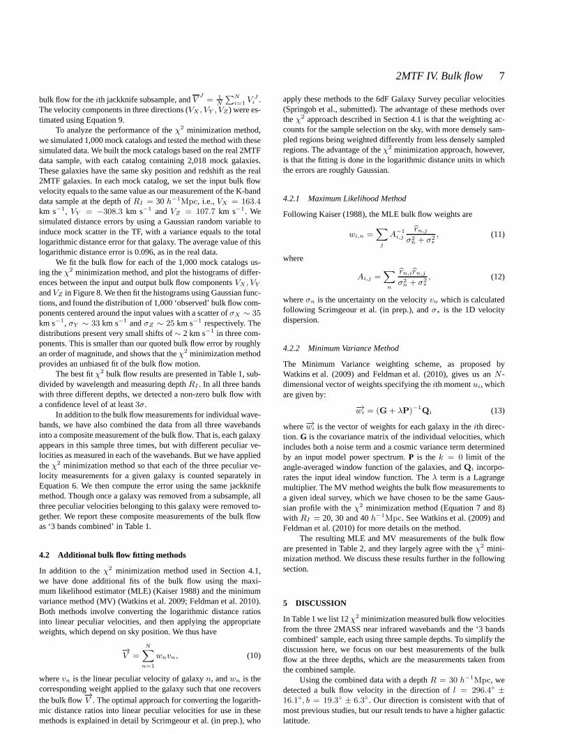
We fit the bulk flow for each of the 1,000 mock catalogs us-ing theχ2 minimization method, and plot the histograms of differ-ences between the input and output bulk flow componentsVX , VY

andVZ in Figure 8. We then fit the histograms using Gaussian func-tions, and found the distribution of 1,000 ‘observed’ bulk flow com-ponents centered around the input values with a scatter ofσX ∼ 35km s−1, σY ∼ 33 km s−1 andσZ ∼ 25 km s−1 respectively. Thedistributions present very small shifts of∼ 2 km s−1 in three com-ponents. This is smaller than our quoted bulk flow error by roughlyan order of magnitude, and shows that theχ2 minimization methodprovides an unbiased fit of the bulk flow motion.

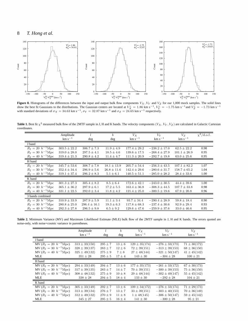
The best fitχ2 bulk flow results are presented in Table 1, sub-divided by wavelength and measuring depthRI . In all three bandswith three different depths, we detected a non-zero bulk flowwitha confidence level of at least3σ.

In addition to the bulk flow measurements for individual wave-bands, we have also combined the data from all three wavebandsinto a composite measurement of the bulk flow. That is, each galaxyappears in this sample three times, but with different peculiar ve-locities as measured in each of the wavebands. But we have appliedtheχ2 minimization method so that each of the three peculiar ve-locity measurements for a given galaxy is counted separately inEquation 6. We then compute the error using the same jackknifemethod. Though once a galaxy was removed from a subsample, allthree peculiar velocities belonging to this galaxy were removed to-gether. We report these composite measurements of the bulk flowas ‘3 bands combined’ in Table 1.

4.2 Additional bulk flow fitting methods

In addition to theχ2 minimization method used in Section 4.1,we have done additional fits of the bulk flow using the maxi-mum likelihood estimator (MLE) (Kaiser 1988) and the minimumvariance method (MV) (Watkins et al. 2009; Feldman et al. 2010).Both methods involve converting the logarithmic distance ratiosinto linear peculiar velocities, and then applying the appropriateweights, which depend on sky position. We thus have

−→V =

N∑

n=1

wnvn, (10)

wherevn is the linear peculiar velocity of galaxyn, andwn is thecorresponding weight applied to the galaxy such that one recoversthe bulk flow

−→V . The optimal approach for converting the logarith-

mic distance ratios into linear peculiar velocities for usein thesemethods is explained in detail by Scrimgeour et al. (in prep.), who

apply these methods to the 6dF Galaxy Survey peculiar velocities(Springob et al., submitted). The advantage of these methods overtheχ2 approach described in Section 4.1 is that the weighting ac-counts for the sample selection on the sky, with more denselysam-pled regions being weighted differently from less densely sampledregions. The advantage of theχ2 minimization approach, however,is that the fitting is done in the logarithmic distance units in whichthe errors are roughly Gaussian.

4.2.1 Maximum Likelihood Method

Following Kaiser (1988), the MLE bulk flow weights are

wi,n =∑

j

A−1i,j

rn,j

σ2n + σ2

∗

, (11)

where

Ai,j =∑

n

rn,irn,j

σ2n + σ2

∗

, (12)

whereσn is the uncertainty on the velocityvn which is calculatedfollowing Scrimgeour et al. (in prep.), andσ∗ is the 1D velocitydispersion.

4.2.2 Minimum Variance Method

The Minimum Variance weighting scheme, as proposed byWatkins et al. (2009) and Feldman et al. (2010), gives us anN -dimensional vector of weights specifying theith momentui, whichare given by:

−→wi = (G+ λP)−1Qi (13)

where−→wi is the vector of weights for each galaxy in theith direc-tion. G is the covariance matrix of the individual velocities, whichincludes both a noise term and a cosmic variance term determinedby an input model power spectrum.P is thek = 0 limit of theangle-averaged window function of the galaxies, andQi incorpo-rates the input ideal window function. Theλ term is a Lagrangemultiplier. The MV method weights the bulk flow measurementstoa given ideal survey, which we have chosen to be the same Gaus-sian profile with theχ2 minimization method (Equation 7 and 8)with RI = 20, 30 and 40h−1Mpc. See Watkins et al. (2009) andFeldman et al. (2010) for more details on the method.

The resulting MLE and MV measurements of the bulk floware presented in Table 2, and they largely agree with theχ2 mini-mization method. We discuss these results further in the followingsection.

5 DISCUSSION

In Table 1 we list 12χ2 minimization measured bulk flow velocitiesfrom the three 2MASS near infrared wavebands and the ‘3 bandscombined’ sample, each using three sample depths. To simplify thediscussion here, we focus on our best measurements of the bulkflow at the three depths, which are the measurements taken fromthe combined sample.

Using the combined data with a depthR = 30 h−1Mpc, wedetected a bulk flow velocity in the direction ofl = 296.4 ±16.1, b = 19.3 ± 6.3. Our direction is consistent with that ofmost previous studies, but our result tends to have a higher galacticlatitude.

8 T. Hong et al.

0

20

40

60

80

100

120

140

-150 -100 -50 0 50 100 150

Count

VXfit

-VXinput

[km s-1

]

VXc = 1.86

σX = 34.63

0

20

40

60

80

100

120

140

-150 -100 -50 0 50 100 150

Count

VYfit

-VYinput

[km s-1

]

VYc = -1.75

σY = 32.87

0

20

40

60

80

100

120

140

160

180

-150 -100 -50 0 50 100 150

Count

VZfit

-VZinput

[km s-1

]

VZc = -1.73

σZ = 24.65

Figure 8. Histograms of the differences between the input and output bulk flow componentsVX , VY andVZ for our 1,000 mock samples. The solid linesshow the best fit Gaussians to the distributions. The Gaussian centers are located atV c

X = 1.86 km s−1, V cY = −1.75 km s−1andV c

Z = −1.73 km s−1

with standard deviations ofσX = 34.63 km s−1, σY = 32.87 km s−1 andσZ = 24.65 km s−1 respectively.

Table 1.Best fitχ2 measured bulk flow of the 2MTF sample in J, H and K bands. The velocity components(VX , VY , VZ ) are calculated in Galactic Cartesiancoordinates.

Amplitude l b VX VY VZ χ2/d.o.f.km s−1 deg deg km s−1 km s−1 km s−1

J bandRI = 20 h−1Mpc 303.5 ± 22.2 306.7± 7.3 11.9± 4.9 177.4 ± 29.2 −238.2 ± 17.0 62.5± 22.2 0.98RI = 30 h−1Mpc 319.0 ± 28.0 297.5± 4.1 18.5± 4.6 139.6 ± 17.5 −268.4 ± 27.9 101.1 ± 26.9 0.95RI = 40 h−1Mpc 319.4 ± 21.3 290.8± 4.2 11.4± 4.7 111.3 ± 20.9 −292.7 ± 19.8 63.0± 25.6 0.95

H bandRI = 20 h−1Mpc 345.7 ± 53.6 308.7± 7.8 18.1 ± 13.9 205.7 ± 54.4 −256.3 ± 43.5 107.1 ± 82.2 1.07RI = 30 h−1Mpc 352.4 ± 34.4 296.9± 5.6 26.8 ± 11.6 142.4 ± 29.6 −280.6 ± 31.7 158.7 ± 65.2 1.04RI = 40 h−1Mpc 319.1 ± 37.4 296.2± 8.3 5.1± 6.1 140.5 ± 51.1 −285.0 ± 28.2 28.4± 33.6 1.00

K bandRI = 20 h−1Mpc 301.3 ± 27.3 305.4± 8.2 8.5± 6.4 172.6 ± 42.1 −243.0 ± 30.5 44.4± 39.6 1.00RI = 30 h−1Mpc 365.1 ± 36.2 297.9± 6.1 17.2± 5.5 163.4 ± 36.8 −308.3 ± 44.5 107.7 ± 33.8 0.98RI = 40 h−1Mpc 331.1 ± 22.5 292.0± 3.4 11.8± 4.2 121.4 ± 25.0 −300.5 ± 19.6 67.9± 20.8 0.96

3 bands combinedRI = 20 h−1Mpc 310.9 ± 33.9 287.9± 5.9 11.1± 3.4 93.7± 34.4 −290.4 ± 28.9 59.8± 18.4 0.90RI = 30 h−1Mpc 280.8 ± 25.0 296.4 ± 16.1 19.3± 6.3 117.8 ± 68.3 −237.4 ± 30.6 92.9± 29.4 0.93RI = 40 h−1Mpc 292.3 ± 27.8 296.5± 9.8 6.5± 9.2 129.6 ± 47.6 −259.9 ± 37.6 33.0± 46.6 0.95

Table 2. Minimum Variance (MV) and Maximum Likelihood Estimate (MLE) bulk flow of the 2MTF sample in J, H and K bands. The errors quoted arenoise-only, with noise+cosmic variance in parentheses.

Amplitude l b VX VY VZ

km s−1 deg deg km s−1 km s−1 km s−1

J bandMV (RI = 20 h−1Mpc) 313± 33(150) 295± 7 13± 6 129± 35(174) −276± 33(173) 71 ± 30(172)MV (RI = 30 h−1Mpc) 328± 39(137) 283± 7 12± 6 72± 39(151) −313± 39(153) 68 ± 36(150)MV (RI = 40 h−1Mpc) 325± 49(132) 275± 9 7± 8 27± 48(144) −321± 50(147) 41 ± 45(142)MLE 351 ± 28 295± 5 17± 4 143± 30 −304± 28 100 ± 21

H bandMV (RI = 20 h−1Mpc) 294± 33(149) 294± 7 13± 6 177± 35(173) −261± 33(172) 67 ± 30(173)MV (RI = 30 h−1Mpc) 317± 39(135) 283± 7 14± 7 70± 39(151) −300± 39(153) 75 ± 36(150)MV (RI = 40 h−1Mpc) 308± 48(132) 275± 9 10± 8 29± 48(144) −302± 49(147) 55 ± 45(142)MLE 338 ± 28 294± 5 18± 4 133± 30 −292± 28 104 ± 21

K bandMV (RI = 20 h−1Mpc) 305± 33(149) 292± 7 13± 6 109± 34(172) −276± 33(174) 71 ± 29(173)MV (RI = 30 h−1Mpc) 313± 39(134) 276± 7 13± 7 33± 39(151) −303± 40(153) 70 ± 36(149)MV (RI = 40 h−1Mpc) 312± 49(132) 270± 9 11± 8 1± 48(145) −306± 50(147) 59 ± 45(142)MLE 345 ± 27 295± 5 16± 4 141± 30 −300± 28 95± 21

2MTF IV. Bulk flow 9

Figure 9. The direction of the measured bulk flow velocities, using an Aitoff projection and Galactic coordinates. The red circle shows the bulk flow directionestimated from ‘3 bands combined’ sample with depthRI = 30 h−1Mpc. The size of the circles indicates the1σ error of the direction. The bulk flowdirections from several previous studies are also plotted for comparison. The references for these literature resultsare listed in Table 3.

Table 3.Bulk flow directions from previous studies

l b Referencedeg deg

2MTF 296.4± 16.1 19.3± 6.3 This workCOMPOSITE 287 ± 9 8± 6 Watkins et al. (2009)FWH10 282± 11 6± 6 Feldman et al. (2010)ND11 276 ± 3 14± 3 Nusser & Davis (2011)DKS11 290+39

−31 20+32−32 Dai et al. (2011)

A1 319± 25 7± 13 Turnbull et al. (2012)MP14 281 ± 7 8+6

−5 Ma & Pan (2014)

We list ourχ2 minimization measured bulk flow directions,along with the results from previous studies in Table 3. An Aitoffprojection of bulk flow directions is also presented in Figure 9.

The expected amplitude of the bulk flow is strongly dependenton the characteristic depth of the galaxies being sampled (Li et al.2012; Ma & Pan 2014). As survey geometry and source selectioncriteria vary greatly between surveys, one must account forthis incomparing the bulk flow amplitude to cosmological expectations.

In theΛCDM model, the variance of the bulk flow velocity ina spherical region R is

v2rms =H2

0f2

2π2

∫W 2(kR)P (k)dk, (14)

wherek is the wavenumber,W (kR) = exp(−k2R2)/2 is theFourier transform of a Gaussian window function,P (k) is the mat-ter power spectrum (we used the matter power spectrum generatedby the CAMB package, Lewis et al. 2000),f = Ω0.55

m is the lineargrowth rate, andH0 is the Hubble constant.

The probability distribution function of the bulk flow V is

(Li et al. 2012)

p(V )dV =

√2

π

(3

v2rms

)3/2

V 2 exp

(−

3V 2

2v2rms

)dV, (15)

The PDF here is normalized. By setting dp(V )/dV = 0, the peakof the distribution can be easily calculated:vpeak =

√2/3vrms.

We adopt this peak velocity as the bulk velocity amplitude pre-dicted by theΛCDM model.

We show the 3 bands combined measurement ofχ2 mini-mization method in Figure 10 together with the model predictedcurve. The1σ variance of the bulk flow velocity is also plottedas a dashed line. Our results agree with the model predicted bulkflow amplitude at the1σ level. Thus, our results support the con-clusions reported by some previous studies (e.g. Dai et al. 2011;Nusser & Davis 2011; Turnbull et al. 2012; Rathaus et al. 2013;Ma & Pan 2014) that the bulk flow detected in the local Universeisconsistent with theΛCDM model.

As a point of comparison, both the MV and MLE results areshown in Table 2. The MV calculation is performed for the same20, 30, and 40 h−1Mpc depths used for theχ2 minimizationmethod, while the MLE method only samples one depth. The mea-surements largely agree with theχ2 minimization results in bothamplitude and direction. A comparison of bulk flow measurementson 2MTF K-band sample is shown in Figures 11 and 12.

6 CONCLUSIONS

The bulk flow motion is the dipole component of the peculiar ve-locity field, thought to be induced by the gravitational attraction oflarge-scale structures. Therefore, its measurement can help to con-strain cosmological models.

10 T. Hong et al.

Figure 11. The direction of the measured bulk flow velocities, using an Aitoff projection and Galactic coordinates. The black, blue, and red circles showthe bulk flow direction determined from the K-band sample by theχ2 minimization (RI = 30 h−1Mpc), Minimum Variance (RI = 30 h−1Mpc), andMaximum Likelihood methods respectively. The size of the circles indicates the1σ error. The literature bulk flow directions are plotted by dashed circles.

0

100

200

300

400

500

600

700

10 20 30 40 50 60

VB

F [

km

s-1

]

R [h-1

Mpc]

Figure 10.The comparison between the bulk flow velocity amplitude fromthe 2MTF sample and theΛCDM prediction using the WMAP-7yr param-eters (Larson et al. 2011). The diamonds with error bars indicate the bulkflow velocity amplitude measured from the 2MTF ‘3 bands combined’ sam-ple using theχ2 minimization method, with the depthRI = 20, 30 and 40h−1Mpc respectively. The solid line shows the theoretical curve and thedashed lines indicate the sample variance at the1σ level.

The 2MTF survey is an all-sky Tully-Fisher survey, using pho-tometric data from the 2MASS catalog and HI data from existingpublished works and new observations. Using this dataset, we havederived peculiar velocities for 2,018 galaxies in the localUniverse(cz 6 10, 000 km s−1). This sample covers all of the sky downto a Galactic latitude|b| = 5, providing better sky-coverage thanprevious surveys.

We applied aχ2 minimization method to the peculiarvelocity catalog to estimate the bulk flow motion. We applied

0

100

200

300

400

500

600

700

10 20 30 40 50 60

VB

F [

km

s-1

]

R [h-1

Mpc]

χ2 minimization

Minimum Variance

Figure 12. The comparison between the bulk flow amplitudes measuredby χ2 minimization method (diamonds) and minimum variance method(squares) on 2MTF K-band sample. The minimum variance method resultsare shifted 1h−1Mpc right to make the comparison clear. The solid lineshows the theoretical curve and the dashed lines indicate the variance at the1σ level.

three Gaussian window functions located at three differentdepths(RI = 20h−1Mpc, 30h−1Mpc, and 40h−1Mpc) to the catalogsgenerated by three near-infrared bands (J, H & K). Our tightestconstraints came from combining the data in all three bands,whichgave us bulk flow amplitudes ofV = 310.9 ± 33.9 km s−1,V = 280.8 ± 25.0 km s−1, andV = 292.3 ± 27.8 km s−1

for RI = 20 h−1Mpc, 30 h−1Mpc and 40h−1Mpc respec-tively. Similar results are found when we apply the maximumlikelihood and minimum variance methods of Kaiser (1988) andWatkins et al. (2009) respectively. We find that these amplitudes

2MTF IV. Bulk flow 11

all agree with theΛCDM model prediction at the1σ level. Thedirections of our estimated bulk flow are also consistent withprevious probes.

The authors gratefully acknowledge Martha Haynes, RiccardoGiovanelli, and the ALFALFA team for supplying the latest AL-FALFA survey data. We thank Yin-zhe Ma for useful commentsand discussions.

The authors wish to acknowledge the contributions of JohnHuchra (1948 - 2010) to this work. The 2MTF survey was initiatedwhile KLM was a post-doc working with John at Harvard, and itsdesign owes much to his advice and insight. This work was partiallysupported by NSF grant AST- 0406906 to PI John Huchra.

Parts of this research were conducted by the Australian Re-search Council Centre of Excellence for All-sky Astrophysics(CAASTRO), through project number CE110001020. TH was sup-ported by the National Natural Science Foundation (NNSF) ofChina (11103032 and 11303035) and the Young Researcher Grantof National Astronomical Observatories, Chinese Academy of Sci-ences.

REFERENCES

Aaronson, M., Huchra, J., Mould, J., Schechter, P. L., & Tully,R. B. 1982, ApJ, 258, 64

Crook, A. C., Huchra, J. P., Martimbeau, N., et al. 2007, ApJ,655,790

Dai, D.-C., Kinney, W. H., & Stojkovic, D. 2011, J. Cosmology& Astroparticle Phys., 4, 15

Djorgovski, S., & Davis, M. 1987, ApJ, 313, 59Dressler, A., Lynden-Bell, D., Burstein, D., et al. 1987, ApJ, 313,42

Efstathiou, G., Ellis, R. S., & Peterson, B. A. 1988, MNRAS, 232,431

Feldman, H. A., Watkins, R., & Hudson, M. J. 2010, MNRAS,407, 2328

Giovanelli, R., Haynes, M. P., Herter, T., et al. 1997, AJ, 113, 53Giovanelli, R., Haynes, M. P., Kent, B. R., et al. 2005, AJ, 130,2598

Haynes, M. P., Giovanelli, R., Martin, A. M., et al. 2011, AJ,142,170

Hong, T., Staveley-Smith, L., Masters, K. L., et al. 2013, MNRAS,432, 1178

Huchra, J. P., Macri, L. M., Masters, K. L., et al. 2012, ApJS,199,26

Hudson, M. J., Smith, R. J., Lucey, J. R., & Branchini, E. 2004,MNRAS, 352, 61

Jarrett, T. H., Chester, T., Cutri, R., et al. 2000, AJ, 119, 2498Kaiser, N. 1988, MNRAS, 231, 149Kochanek, C. S., Pahre, M. A., Falco, E. E., et al. 2001, ApJ, 560,566

Larson, D., Dunkley, J., Hinshaw, G., et al. 2011, ApJS, 192,16Lewis, A., Challinor, A., & Lasenby, A. 2000, ApJ, 538, 473Li, M., Pan, J., Gao, L., et al. 2012, ApJ, 761, 151Ma, Y.-Z., Branchini, E., & Scott, D. 2012, MNRAS, 425, 2880Ma, Y.-Z., & Pan, J. 2014, MNRAS, 437, 1996Ma, Y.-Z., & Scott, D. 2013, MNRAS, 428, 2017Masters, K. L., Crook, A., Hong, T., et al. 2014, MNRAS, 443,1044

Masters, K. L., Springob, C. M., Haynes, M. P., & Giovanelli,R.2006, ApJ, 653, 861

Masters, K. L., Springob, C. M., & Huchra, J. P. 2008, AJ, 135,1738

Mathewson, D. S., Ford, V. L., & Buchhorn, M. 1992, ApJS, 81,413

Nusser, A., & Davis, M. 2011, ApJ, 736, 93Paturel, G., Theureau, G., Bottinelli, L., et al. 2003, A&A,412,57

Phillips, M. M. 1993, ApJL, 413, L105Press, W. H., & Schechter, P. 1974, ApJ, 187, 425Rathaus, B., Kovetz, E. D., & Itzhaki, N. 2013, MNRAS, 431,3678

Springob, C. M., Haynes, M. P., Giovanelli, R., & Kent, B. R.2005, ApJS, 160, 149

Springob, C. M., Masters, K. L., Haynes, M. P., Giovanelli, R., &Marinoni, C. 2007, ApJS, 172, 599

Staveley-Smith, L., & Davies, R. D. 1989, MNRAS, 241, 787Strauss, M. A., & Willick, J. A. 1995, Phys. Rep., 261, 271Theureau, G., Bottinelli, L., Coudreau-Durand, N., et al. 1998,A&AS, 130, 333

Theureau, G., Hanski, M. O., Coudreau, N., Hallet, N., & Martin,J.-M. 2007, A&A, 465, 71

Theureau, G., Coudreau, N., Hallet, N., et al. 2005, A&A, 430,373

Tully, R. B., & Fisher, J. R. 1977, A&A, 54, 661Turnbull, S. J., Hudson, M. J., Feldman, H. A., et al. 2012, MN-RAS, 420, 447

Watkins, R., Feldman, H. A., & Hudson, M. J. 2009, MNRAS,392, 743

APPENDIX A: NEW INTRINSIC ERROR ESTIMATION

As described in section 2.1, Masters et al. (2008) estimatedthe in-trinsic errors of the Tully-Fisher relation using the 888-galaxy tem-plate sample with I-band axis-ratios. However, we have adopted the2MASS co-added axis-ratio for the 2MTF sample. Thus, we mustmake a new estimate of the intrinsic scatter in the TF relation, ap-propriate for the co-added axis ratios. We have calculated the newintrinsic errors by subtracting the observed error components fromthe total scatter of the distribution.

We assume that a proper error estimation should approxi-mately match the total scatter of the data sample:

σ2 ∼ ǫ2total = ǫ2wid + ǫ2ran + ǫ2mag + ǫ2inc + ǫ2int, (A1)

whereσ is the scatter of the data points related to the Tully-Fishertemplate,ǫwid is the error of the HI widths,ǫran = 268 km s−1 isthe assumed mean rms of velocities for field galaxies (see detailsin Appendix B),ǫmag is the error on the 2MASS magnitudes,ǫincis the error introduced by the 2MASS co-added inclinations,ǫint isthe intrinsic error of the Tully-Fisher relation. All errors and scatterin Equation A1 are in logarithmic units.

The residual component or intrinsic error is

ǫ2int ∼ σ2 −(ǫ2wid + ǫ2ran + ǫ2mag + ǫ2inc

). (A2)

We assume a linear relation between the intrinsic error andlogarithmic HI widths logW

ǫint = a logW + b, (A3)

wherea andb are free parameters.The final results are the intrinsic error terms reported by Equa-

tion 3. We show the error components along with the total scatter of

12 T. Hong et al.

0

0.1

0.2

0.3

0.4

0.5

0.6

0.7

0.8

0.9

1

2.1 2.2 2.3 2.4 2.5 2.6 2.7 2.8 2.9

Err

or/

Sca

tter

[m

ag]

log (W/km s-1

)

scattertotal

magnituderandom motion

widthinclination

intrinsic-new

Figure A1. A plot of different error components of the K-band data as afunction of the logarithmic HI width. The blue dashed line indicates thenew intrinsic error term. The red line shows our estimate of the final totalerror in the data, which matches the observed scatter of the sample well.

the K-band sample in the Figure A1. Using the new intrinsic error,the total error closely matches the total scatter.

APPENDIX B: THE RANDOM MOTION OF GALAXIES

Ideally, the intrinsic error of the Tully-Fisher relation would be esti-mated using a galaxy cluster sample. All of the galaxies in the samecluster are assumed to be at the same distance, thus subtracting outthe individual motions of the galaxies themselves. However, whenestimating the new intrinsic error term, we used the data of 2,018field galaxies. The uncorrected random motions of these galaxieswould introduce a spurious component into the scatter of theTully-Fisher relation.

To remove this effect, we need to estimate the mean randommotion of galaxies in our sample. We start by calculating thepe-culiar velocity of the field galaxies using the Tully-Fisherrela-tion template from Equation 1. Instead of the logarithmic quantitylog(dz/dTF), a linear low redshift approximation

vpec = cz(1− 10

∆M

5

), (B1)

is adopted to generate the peculiar velocities of galaxies.We thenplace the galaxies onto the redshift - peculiar velocity diagram Fig-ure B1, and calculate peculiar velocity scatter in redshiftbins ofwidth 1000 km s−1. As expected, the scatter increases with red-shift, owing to the fact that most of the observational errors scalewith distance. To find the pure random motion velocity of the galax-ies, we do a linear fit to the scatter as a function of redshift,andextended the linear relation tocz = 0 km s−1. We adopt this zeropoint as the underlying rms of our velocities. As shown in Fig-ure B2, we foundvran = 268 km s−1, which is close to the com-monly used value ofvran = 300 km s−1(e.g., Strauss & Willick1995; Masters et al. 2006).

-5000

-4000

-3000

-2000

-1000

0

1000

2000

3000

4000

0 2000 4000 6000 8000 10000

Pec

uli

ar V

elo

city

[k

m s

-1]

cz [km s-1

]

Figure B1. Peculiar velocities vs. redshift for the 2,018 2MTF field galax-ies.

200

400

600

800

1000

1200

1400

1600

1800

0 2000 4000 6000 8000 10000

Sca

tter

[k

m s

-1]

cz [km s-1

]

y = a + b*xa = 268.0540 ± 1.1582b = 0.1401 ± 0.0002

Figure B2. Mean scatter of peculiar velocity as a function of redshift,withthe best fit linear relation superimposed.