3-cash flow, interest and equivalence€¦ · a cash flow diagram is created by first drawing a...

Chapter – 2 : Cash Flow, Interest and Equivalence

Economics for Engineers (3140911)

What is cash flow?

Word “cash” in economics represent the cash on hand i.e. liquidity. It is sterile (harmless) asset but

ideally it does not generate any wealth.

When cash is invested in some non-cash asset i.e. material, equipment, gold, shares, land,

infrastructure, fixed deposit etc. then use of asset or increased price of asset generates wealth.

Thus one can say profitability and liquidity are inversely proportional in relation i.e. high liquidity,

low profitability.

For any engineering project cash on hand is life of business but profitability is also the main

component.

Hence cash – non cash – cash cycle i.e. circulation of cash is an important and unavoidable need of

project/business.

For any cash flow analysis, bank balance is considered as “near cash” balance. Thus both the

balances cash on hand and cash balance in bank is considered jointly.Economics for Engineers (3140911)

Types of cash flow

Cash flow is basically classified as

o Cash Inflows

It is the cash receipts i.e. increase the cash on hand.

It has further two sub classification

Recurring cash inflow i.e. daily cash sales, monthly income, rent of property

Non recurring cash inflow i.e. salvage value of machine, insurance settlement, business separation

o Cash Outflows

It is the cash payment i.e. reduces the cash on hand

It has further two sub classification

Recurring cash outflow i.e. purchase of raw material, salary of employee, electricity bill

Non recurring cash outflow i.e. purchase of assets, machinery, equipment, vehicle, infrastructure,

land


Cash flow diagram

It is financial tool that represents the cash flow at different time interval. It characterizes the cash

inflows and cash outflow for short term revenue transactions and long term capital transactions.

The costs and benefits of engineering projects occur over time and are summarized on a cash flow

diagram (CFD). It illustrates the size, sign, and timing of individual cash flows.

A cash flow diagram is created by first drawing a segmented time-based horizontal line, divided into

time units. The time units on the CFD can be years, months, quarters, or any other consistent time

unit.

Then at each time at which a cash flow will occur, a vertical arrow is added pointing down for costs

and up for revenues or benefits. These cash flows are drawn to scale.

Unless otherwise stated, cash flows are assumed to occur at time 0 or at the end of each period.

Visually cash flow diagram represents the cash income and cash expenses over the time interval i.e.

one year.


Cash flow diagram

Particulars t0 t1 t2 t3 tn

Non – Recurring Initial Investment (↓) ---- ---- ---- Terminal Revenue (↑)

Recurring ---- Sales (↑) Sales (↑) Sales (↑) Sales (↑)

---- Deprecation (↑) Deprecation (↑) Deprecation (↑) Deprecation (↑)

Expenses (↓) Expenses (↓) Expenses (↓) Expenses (↓)

Tax (↓) Tax (↓) Tax (↓) Tax (↓)

FD Interest (↑) FD Interest (↑) FD Interest (↑) FD Interest (↑)

Loan Installment (↓) Loan Installment (↓) ---- ----

Total

% Discount

Net discounted

cash flow


Cash flow diagram

Example – 1

Develop a cash-flow diagram for five year life of the project proposed by a firm where an investment of

INR 10,000 can be made that will produce uniform annual revenue of INR 5,310 for five years and then

have a market (recovery) value of INR 2,000 at the end of year (EOY) five. Annual expenses will be INR

3,000 at the end of each year for operating and maintaining the project. Draw a cash-flow diagram for

the five-year life of the project.

Year Amount (INR)

1 10,000 (↓)

2 5,310 (↑) 3000 (↓)

3 5,310 (↑) 3000 (↓)

4 5,310 (↑) 3000 (↓)

5 5,310 (↑) 3,000 (↓) 2,000 (↑)

1 2 30 4 5

10,000

3,000

2,000

5,310


Cash flow diagram

Example – 2

Develop a cash-flow diagram for nine year life of the project proposed by a firm where an initial project

cost is of INR 80,000. annual operating cost is INR 15,000. major repair cost at the end of 5th year is INR

16,000 and salvage value at the end of project life is INR 8,000.Draw a cash-flow diagram at end-of year

(EOY) of the project.

Year Amount (INR)

1 80,000 (↓)

2 15,000 (↓)

3 15,000 (↓)

4 15,000 (↓)

5 15,000 (↓) 16,000 (↓)

6 15,000 (↓)

7 15,000 (↓)

8 15,000 (↓)

9 15,000 (↓) 8,000 (↑)

1 2 30 4 5 6 7 8 9

80,000 16,000

15,000

8,000


Cash flow diagram

The transactions in any engineering projects are

o Initial investment

o Periodic maintenance expenses

o Earning and savings

o Salvage or resale of equipment

Hence cash flow diagram helps to determine

o Breakeven point

o Scheduling of contractual payment like interest and principal amount

o Cash profit


Categories of cash flows

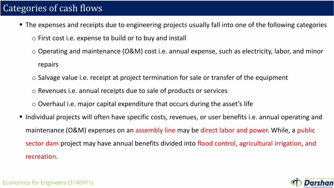
The expenses and receipts due to engineering projects usually fall into one of the following categories

o First cost i.e. expense to build or to buy and install

o Operating and maintenance (O&M) cost i.e. annual expense, such as electricity, labor, and minor

repairs

o Salvage value i.e. receipt at project termination for sale or transfer of the equipment

o Revenues i.e. annual receipts due to sale of products or services

o Overhaul i.e. major capital expenditure that occurs during the asset’s life

Individual projects will often have specific costs, revenues, or user benefits i.e. annual operating and

maintenance (O&M) expenses on an assembly line may be direct labor and power. While, a public

sector dam project may have annual benefits divided into flood control, agricultural irrigation, and

recreation.


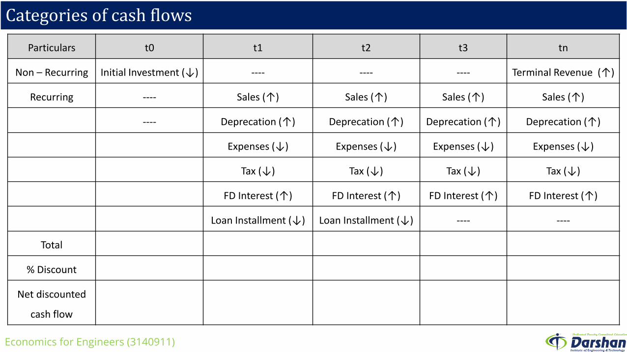
Categories of cash flows

Particulars t0 t1 t2 t3 tn

Non – Recurring Initial Investment (↓) ---- ---- ---- Terminal Revenue (↑)

Recurring ---- Sales (↑) Sales (↑) Sales (↑) Sales (↑)

---- Deprecation (↑) Deprecation (↑) Deprecation (↑) Deprecation (↑)

Expenses (↓) Expenses (↓) Expenses (↓) Expenses (↓)

Tax (↓) Tax (↓) Tax (↓) Tax (↓)

FD Interest (↑) FD Interest (↑) FD Interest (↑) FD Interest (↑)

Loan Installment (↓) Loan Installment (↓) ---- ----

Total

% Discount

Net discounted

cash flow


Why money has a time value ?

The majority of engineering economy involves commitment of capital i.e. wealth in the form of

money or property that is used to produce more wealth for extended periods of time, so the

effect of time is an integral part of any engineering investment.

In this regard, it is recognized that a INR today is worth more than a INR one or more years from

now due to the interest or profit it can earn.

Therefore, money has a time value.

If money remains un-invested i.e. in a closet, value is lost. Money changes in value not only

because of interest rates, inflation or deflation but currency exchange rates also cause money to

change in value.

We often find financial flashes of any alternative occur over a large period or short period of time.

One can simply add up the various sums of money and obtain a net result for short period of

time. But for long period of time money can not be treated this way.


Why money has a time value ?

For example

Which would one can prefer, INR 100 cash today or the assurance of receiving INR 100 a year

from now?

One may decide to have INR 100 now because that is one way to be certain of receiving it. But

suppose one may be convinced to receive the INR 100 one year later, then also it is more

desirable to receive the INR 100 now rather than a year.

Because one can have use of money for an extra year i.e. deposit in a bank.

If the current interest rate is 9% per year and one put INR 100 into the bank for one year. After

one year one will get original INR 100 + interest INR 9 = Total INR 109.

Hence it is proven that money has time value in the form of the willingness of banks, businesses

and people who can pay interest for the use of money.

The importance of interest is confirmed by banks and savings institutions continuously offering to

pay for the use of people’s money.


Why consider return to capital?

Money is such a valuable asset that people are willing to pay to have money available for their

use. It can be rented in roughly the same way one can rents an apartment. In case of money, the

charge is called interest or profit instead of rent.

In engineering economics return to capital in the form of interest and profit is an essential

ingredient.

An interest and profit pays to the providers of capital for previous its use during the time the

capital is being used. A return on capital is an incentive to accumulate capital by savings, thus

postponing immediate consumption in favor of creating wealth in the future.

An interest and profit are payments for the risk the investor takes in permitting another person

or an organization to use his or her capital.

Whenever capital is required in engineering and other business projects and ventures, it is

essential that proper consideration be given to its cost i.e. time value.


Why consider return to capital?

For example

In typical situations, investors must decide whether the expected return on their capital is

sufficient to justify business into a proposed project or venture.

If capital is invested in a project, investors may expect, minimum return to capital at least equal

to the amount they have sacrificed by not using it in some other available opportunity of

comparable risk.

This interest or profit available from an alternative investment is the opportunity cost of using

capital in the proposed undertaking.

Thus, whether borrowed capital or equity capital is involved, there is a cost for the capital

invested in the sense that the project and venture must provide a sufficient financially attractive

return to suppliers of money or property.


The origins of interest

Like taxes, interest has existed from earliest recorded human history in Babylon in 2000 B.C.

Earliest instances, interest was paid in money for the use of grain or other commodities that were

borrowed; it was also paid in the form of grain or other goods.

Many existing interest practices branch from early customs in the borrowing and repayment of

grain and other crops.

History also reveals that the idea of interest became so well established that a firm of international

bankers existed in 575 B.C. with home offices in Babylon.

The firm’s income was derived from the high interest rates it charged for the use of its money for

financing international trade.

In early history, typical annual rates of interest on loans of money were 6% to 25%, and legally

sanctioned rates as high as 40% were permitted in some instances.

The charging of exorbitant interest rates on loans was termed moneylending, and prohibition of

moneylending is found in the Bible.Economics for Engineers (3140911)

The origins of interest

In early history, typical annual rates of interest on loans of money were 6% to 25%, and legally

sanctioned rates as high as 40% were permitted in some instances.

During the middle ages, interest taking on loans of money was generally banned on holy

grounds.

In 1536, the protestant theory of moneylending was established by John Calvin, and it disproved

the idea that interest was unlawful .

Consequently, interest taking again became viewed as an essential and legal part of doing

business and published interest tables became available to the public.

Now a days for return to capital in terms of interest is calculated by means of

o Simple Interest

o Compound Interest


Simple Interest

It is the interest that is computed only on the original sum, not on accrued interest. If

P = Loan a present sum of money

i = Simple annual interest rate

N = Period in years

I = Total interest earned at the end of N year

F= Amount of money payable at the end of N year

I= P i N

F=P + I = P +(P i N)= P(1+i N)

Simple interest is not used in modern commercial practice because cumulative amount of

interest owed is a linear function of time until the principal and interest is repaid, usually not

until the end of period N. So, lenders seldom agree to make simple interest loans.


Simple Interest

Example : 1

If INR 1,000 were loaned for three years at a simple interest rate of 10% per year. Calculate (i)

Simple interest earned (ii) Amount of money payable at the end of three year

P = 1000 INR

i = 10 % = 0.1

N = 03

I= P i N = 1000 0.1 03 = 300 INR

F=P + I = 1000 + 300 = 1300 INR


Simple Interest

Example : 2

If a someone is agreed to loan a friend INR 5000 for 5 years at a simple interest rate of 8% per

year. How much simple interest will he receive from the loan? How much will a friend pay him

at the end of 5 years?

P = 5000 INR

i = 8 % = 0.08

N = 05

I= P i N = 5000 0.08 05 = 2000 INR

F=P + I = 5000 + 2000 = 7000 INR


Compound Interest

Whenever the interest charge for any interest period i.e. a year is based on the remaining

principal amount plus any accumulated interest charges up to the beginning of that period, the

interest is said to be compound. In this way, compound interest can be thought of as interest on

top of interest.

Difference of amount of money payable at the end of N year will be much greater for larger

amounts of money, higher interest rates, or greater numbers of interest periods. Compound

interest is much more common in practice than simple interest.

If


i = Compound annual interest rate

N = Period in years F= P(1+i) N

I = Total interest earned at the end of N year

F= Amount of money payable at the end of N year


Compound Interest

Period (Years)

Amount Owed at Beginning of Period (INR)

Interest Amount for Period (INR)

Amount Owed at End of Period (INR)

1 P1 I 1= P 1 i F1 = P1 + I1

2 F1 I 2= F 1 i F2 = F1 + I2

3 F2 I 3= F 2 i F3 = F2 + I3

N FN-1 I N= F N-1 i FN = FN-1 + IN


Compound Interest

Example : 1

If INR 1,000 were loaned for three years at a simple interest rate of 10% per year. Calculate (i)

Compound interest earned (ii) Amount of money payable at the end of three year

P = 1000 INR F= P(1+i) N= 1000 (1+0.1)3= 1331

i = 10 % = 0.1

N = 03

Period (Years)




1 1000 I 1= 1000 0.1 = 100 F1 = 1100

2 1100 I 2= 1100 0.1 = 110 F2 = 1210

3 1210 I 3= 1210 0.1 = 121 F3 = 1331


Compound Interest

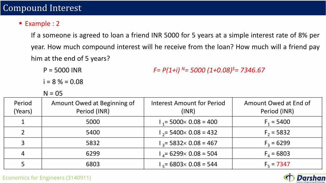
Example : 2

If a someone is agreed to loan a friend INR 5000 for 5 years at a simple interest rate of 8% per

year. How much compound interest will he receive from the loan? How much will a friend pay

him at the end of 5 years?

P = 5000 INR F= P(1+i) N= 5000 (1+0.08)5= 7346.67

i = 8 % = 0.08

N = 05

Period (Years)




1 5000 I 1= 5000 0.08 = 400 F1 = 5400

2 5400 I 2= 5400 0.08 = 432 F2 = 5832

3 5832 I 3= 5832 0.08 = 467 F3 = 6299

4 6299 I 4= 6299 0.08 = 504 F4 = 6803

5 6803 I 5= 6803 0.08 = 544 F5 = 7347


Repaying a Debt

Debt fund is contractual amount raised by the borrowers at a committed interest rate and the

debt repayments of principal amount along with the outstanding interest.

Debt funds are invested in certain typical projects having different type of cash flow. But cash

flow from project investments are uncertain so, borrower agrees to make debt repayment as per

cash flow pattern suitable for the debt payment.

There are a many ways in which debts are repaid

1. Single debt situation

2. Multiple debts situation

3. Equity conversion method

4. Call option method for debenture redemption

5. Purchase of own debentures from market for cancellations


Repaying a Debt - Single Debt Situation

There are certain huge and costly products where in the single debt is raised under one

contracting involving huge repayment amount along with interest.

This kind of funds are usually raised by bank or consortium (group) lending.

One main bank correlates other banks for the loan amount. One head bank negotiates with the

borrower. The mode of repayment in single debt situation can be made under following ways.

a) Sinking fund method

b) Serial repayment of debt

Constant Principal

Interest Only

Constant Payment

All at Maturity


Repaying a Debt - Single Debt Situation (Sinking fund method)

Engineering projects has long development period i.e. power plant, dam, highway etc. The cash

inflow starts after a long lapse of time. Hence debt financing for this kind of projects are done

under sinking (falling) fund method.

In this method, a fixed depreciation charges are made every year and interest compounded on it

annually.

The constant depreciation charges are such that total of annual instalment plus the interest

accumulations equal to the cost of replacement of equipment after its useful life.

If


i = Annual interest rate

N = Period in years

S = Scrap value after useful life

q = Amount set aside as depreciation charge every year

P-S = Cost of replacement

Rate of depreciation and interest are selected such that amount (P-S) is available after N year.Economics for Engineers (3140911)

Repaying a Debt - Single Debt Situation (Sinking Fund Method)

Amount q at annual interest rate i becomes Q= q(1+i) N at the end of n year.

Proof:

At the end of first year, amount = q + iq = q(1+i)

At the end of second year, amount = q(1+i) + iq(1+i) = q(1+i)(1+i)=q(1+i)2

At the end of third year, amount = q(1+i)2 + iq(1+i)2 = q(1+i)2(1+i)=q(1+i)3

At the end of n year, amount = q(1+i)n-1 + iq(1+i)n-1 = q(1+i)n-1(1+i)=q(1+i)N

In another words,

Amount q deposited at the end of first year will earn compound interest for n-1 year and becomes q(1+i)N-1

Amount q deposited at the end of second year will earn compound interest for n-2 year and becomes q(1+i)N-2

Amount q deposited at the end of third year will earn compound interest for n-3 year and becomes q(1+i)N-3

Amount q deposited at the end of n-1 year will earn compound interest for 1 year and becomes q(1+i)N-(N-1)= q(1+i)

Total fund after n years

𝐶 = 𝑞 1 + 𝑖 𝑁−1+𝑞 1 + 𝑖 𝑁−2+ ----------+𝑞 1 + 𝑖 =𝑞 1+𝑖 𝑁−1

𝑖



This total fund must be equal to the cost of replacement of equipment

Hence sinking fund

The value of q gives the uniform annual depreciation charge.

Sinking fund factor

This method does not find frequent application in practical depreciation accounting, it is the

fundamental method in making economy studies.

𝑃 − 𝑆 =𝑞 1 + 𝑖 𝑁 − 1

𝑖

𝑞 = 𝑃 − 𝑆𝑖

1 + 𝑖 𝑁 − 1

=𝑖

1 + 𝑖 𝑁 − 1



Example : 1

If INR 15,60,000 is owned and has a salvage value of INR 60,000 at the end of 25 years. Annual

compound interest rate is 5%. What will be depreciated value of the equipment at the end of 20

Year

Sinking fund,

Sinking fund at the end of 20 years,

Value of plant after 20 years = 15,60,000 – 10,39,362 = 5,20,638

𝑞 = 𝑃 − 𝑆𝑖

1+𝑖 𝑁−1= 1560000 − 60000

0.05

1+0.05 25−1= 31,433

C = q 1+i N−1

i=

31,433 1+0.05 20−1

0.05=10,39,362


Repaying a Debt - Serial Repayment of Debt (Constant principal)

In this plan, 1/nth of the principal plus interest due at the end of the year for the use of money to

that point is paid each year. The series of payments continues each year until the loan is fully

repaid at the end of the defined period.

Example : 1

If INR 5,000 is owned and it is to be paid in five years together with 8% interest rate.

Period (Years)

Amount Owed at Beginning of Period

(a)

Interest Owed forthat Year

(b)

Total Owed at End of Period

(c) = (a) + (b)

Principal Payment(d) = P/N

Total End of Period Payment

(e) = (b) + (d)

1 5000 5000 0.08 = 400 5400 1000 1400

2 4000 4000 0.08 = 320 4320 1000 1320

3 3000 3000 0.08 = 240 3240 1000 1240

4 2000 2000 0.08 = 160 2160 1000 1160

5 1000 1000 0.08 = 80 1080 1000 1080

Total 1200 5000 6200


Repaying a Debt - Serial Repayment of Debt (Interest only)

In this plan only the interest due is paid each year, with no principal payment

Example : 1


Period (Years)


(a)


(b)


(c) = (a) + (b)

Principal Payment(d)


(e) = (b) + (d)

1 5000 5000 0.08 = 400 5400 0 400

2 5000 5000 0.08 = 400 5400 0 400

3 5000 5000 0.08 = 400 5400 0 400

4 5000 5000 0.08 = 400 5400 0 400

5 5000 5000 0.08 = 400 5400 5000 5400

Total 2000 5000 7000


Repaying a Debt - Serial Repayment of Debt (Constant Payment)

In this plan equal end-of-year payments are made i.e. INR 1252.

Example : 1


Period (Years)


(a)


(b)


(c) = (a) + (b)

Principal Payment(d)


(e) = (b) + (d)

1 5000 5000 0.08 = 400 5400 852 1252

2 4148 4148 0.08 = 331 4479 921 1252

3 3227 3227 0.08 = 258 4385 994 1252

4 2233 2233 0.08 = 178 2411 1074 1252

5 1159 1159 0.08 = 93 1252 1159 1252

Total 1260 5000 6260


Repaying a Debt - Serial Repayment of Debt (All at Maturity)

In this plan, no payment is made until the end of Year 5, when the loan is completely repaid.

Example : 1


Period (Years)


(a)


(b)


(c) = (a) + (b)

Principal Payment(d) = P/N


(e) = (b) + (d)

1 5000 5000 0.08 = 400 5400 0 400

2 5400 5400 0.08 = 432 5832 0 432

3 5832 5832 0.08 = 467 6299 0 467

4 6299 6299 0.08 = 504 6803 0 504

5 6803 6803 0.08 = 544 7347 5000 5544

Total 2347 5000 7347


Repaying a Debt - Multiple Debts Situation

When dozes of multiple debts (use of credit card) are raised with different interest rate and different

maturity amount, then debts are classified for the organization of repayment.

Usually methods used for repayment of multiple debts situation are

Avalanche Method

In this method various category of debts are arranged in descending (downward) order of interest rate.

Highest interest rate is put first and then various debt with its interest rates are arranged from high to low.

First highest interest rate debts are repaid. Various interest rates are arranged in sequence so sometimes

this method is called Staking Method.

Snow Ball Method

In this method various category of debts are arranged in ascending (upward) order of total dozes of diverse

debt.

Lowest debt amount is put first and then various debt with sequential higher amount are arranged from

low to high. Debt staking is made on the basis of amount payable.

The debt with least amount is paid first and then debt with next higher order is repaid sequentially.


Repaying a Debt - Equity Conversion Method

In this method debt are not actually repaid in cash but they are converted into some other attractive form

of investment.

Private sector companies uses this method through the issue of convertible debentures i.e. treasure bonds

or treasure bill.

Convertible debentures are issued in equity (parity) share after lapse of certain time. Conversion ratio and

conversion price are specified at the time of issue.

Equity share capital is permanent funding to the business. Once the debentures are converted into shares

they need not to be repaid.

This is a specialized method of debt redemption. Such debentures are issued by the companies by calling

debentures back when company has comfortable liquidity (enough cash) and prevailing market price is

favorable.

Usually call option period is after lapse of the issues date, any time after completion of 3th year till

maturity. Call option is always clarified at the time of issue. Company’s debt is repaid when call option is

exercised.


Repaying a Debt – Call Option of Debenture Redemption

Convertible debentures are either partly convertible or fully convertible.

In case of partly convertible debentures, non convertible part remains in debt form and need to

repay in cash.

Example : 1

If company issued 10% debentures each of INR 500, they are convertible into equity share at

price of INR 125 per share any time after 3rd year before 5th year.

Convertible debentures issued by good companies carry little lower rate of interests before

conversion they are traded at premium as per the rise in market price of the equity share in stock

market.

Usually IT companies have issued convertible debentures. Reliance Industries Limited is the

pioneer company in India to make this method of debt repayment.


Repaying a Debt – Purchase of Own Debenture from Market

In India and some other countries, the debenture issuing company whose debenture are traded

in stock market are allowed to buy its own debenture from market if market price of bond is

favorable.

Example : 1

If INR 100, 12% bonds are traded at INR 80 per debenture, then for company it is beneficial to

buy it from market and cancel them.

Thus the company will be benefited through buying and cancelling rather than repaying them on

maturity.

It is the popular method of debt repaying.


Nominal interest rate

Interest is the financial service charge, charged by lender from the borrower for using the money for

the contractual period. Initial money provided is called principal amount and service charge is called

interest charge.

If as fix percentage interest 12% which signifies that borrower have to pay INR 12 as financial service

charge on INR 100 principal amount for 1 year. Hence, usual interest rate in the market on the date of

transaction is called nominal interest rate.

Nominal interest rates are usual rates prevailing the country’s economy. It is guided by RBI periodic

monetary policy. It is linked to bank rate i.e. interest charged by RBI from scheduled banks for RBI

lending made to them.

Example - 1

If bank pays 21

2% interest every 6 months. What will be the nominal interest rate par year?

r = Duration of interest payment in a year x interest rate = 2 x 2.5% = 5%



Nominal interest rate differences are caused due to

Term structure : Nominal interest rate is higher on long term security i.e. 12% on 10 year while

lower on short term 6% on 182 days on commercial paper.

Brand Image : Government treasure bond has 9% rate for 10 year while private company

debenture has 12% rate for 10 years.

Risk Involved in Borrower’s Project: High risk project lending has little higher nominal interest

rate i.e. 15% compared to usual rate i.e. 12%. Difference in nominal interest rate is called risk

premium i.e. 3%.

Current Economic Condition : Booms and depression in market governs the interest rate. In

the boom period, nominal interest rate are higher and in the depression it tend to be lower.



The nominal interest charges are fixed and they are classified under different financial

transactions such as

a) Bank lending charge

Bank’s main function is to borrow and/or land the money. For each transaction, the nominal

interest rates are defined contract.

Bank lands money in terms of

• Long term bank loan

• Short term overdraft

• Cash-credit

• Bill discount

• Factoring



b) Issue of debt instrument by government or company

Debt instrument is financial instruments issued by borrower with the fixed face value (INR

100, INR 1000, INR 25000 etc.), terms in year ( 1 year, 5 year, 10 year etc.) and nominal

interest rate printed on it.

Long term debt instruments issued by private company is known as debentures.

Long term fund raised by government from public by issuing debt instrument is known as

Treasury Bond. Government bond has specified nominal interest rate, face value of treasury

bond and term structure in year printed on it.

Nominal interest rate is contemporary (current) interest rate and remains fixed till maturity

period of financial contract.


Effective interest rate

Effective interest rate is calculated on the basis of nominal interest rate, that has tendency to be

a fixed contractual rate.

For dynamic business condition, effective rate are to be little higher or lower than nominal

interest rate. Variation in nominal interest rate and effective interest rate are caused by issue

cost, redemption premium, tax advantages and yield rate.

If

r = Nominal interest rate per interest period (usually one year)

i = Effective interest rate per interest period

m = Number of compounding sub periods per time period

Effective annual interest rate, Ia= 1 +𝑟

𝑚

𝑚

− 1 = 1 + 𝑖 𝑚 − 1



The difference between nominal interest and effective interest rate are due to some factors as

mentioned below.

a) Issue cost to borrower

A one time issue cost is incurred by the borrower on the time of issue of financial debt for

example processing fees taken by bank at the time of issue of term loan.

This increases the borrowing nominal interest rate to the borrower.

Example : 1

If a debentures of INR 1,00,000 each of INR 100 with 12% coupon rate redeemable after 10 years

and incurred INR 8000 issue or floatation (promotion) costs. What will be the effective interest

rate?

% Increase =Floatation Cost

Debentures Cost×

1

n× 100=

8000

100000×

1

10× 100 = 0.8%

% Effective Interest Rate = Nominal Interest Rate +% Increase = 12 + 0.8 = 12.8%



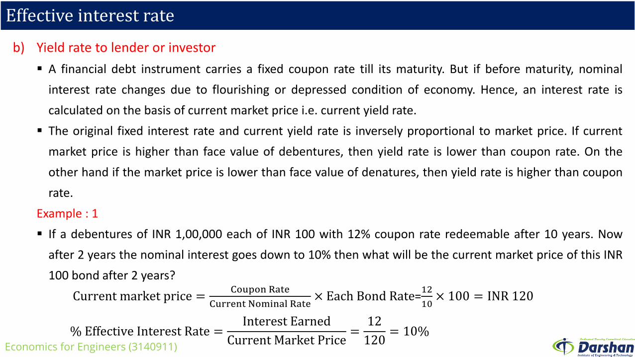
b) Yield rate to lender or investor

A financial debt instrument carries a fixed coupon rate till its maturity. But if before maturity, nominal

interest rate changes due to flourishing or depressed condition of economy. Hence, an interest rate is

calculated on the basis of current market price i.e. current yield rate.

The original fixed interest rate and current yield rate is inversely proportional to market price. If current

market price is higher than face value of debentures, then yield rate is lower than coupon rate. On the

other hand if the market price is lower than face value of denatures, then yield rate is higher than coupon

rate.

Example : 1

If a debentures of INR 1,00,000 each of INR 100 with 12% coupon rate redeemable after 10 years. Now

after 2 years the nominal interest goes down to 10% then what will be the current market price of this INR

100 bond after 2 years?

Current market price =Coupon Rate

Current Nominal Rate× Each Bond Rate=

12

10× 100 = INR 120

% Effective Interest Rate =Interest Earned

Current Market Price=

12

120= 10%



c) Tax advantages to the borrower

Interest on debt is allowed as deductible expenses for income tax payers. So the effective cost of

borrowing to the borrower is reduced by tax advantages on debt funding.

Example : 1

If a debentures of INR 1,00,000 each of INR 100 with 12% coupon rate redeemable after 10

years. Company falls under 30% tax slab. What will be effective interest rate?

% Effective Interest Rate = Coupon Rate (1- Tax Rate) = 0.12 (1-0.3) = 0.084 = 8.4%


3-cash flow, interest and equivalence€¦ · a cash flow diagram is created by first drawing a...

Documents