3 chapter 2: mitigation pathways compatible with 1.5°c in ... · 1 in comparison to a 2°c limit,...
TRANSCRIPT
Approval Session Chapter 2 IPCC SR1.5
Do Not Cite, Quote or Distribute 2-1 Total pages: 112
1
2
Chapter 2: Mitigation pathways compatible with 1.5°C in the context of sustainable 3
development 4
5
6
Coordinating Lead Authors: Joeri Rogelj (Belgium/Austria), Drew Shindell (USA), Kejun Jiang (China) 7
8
Lead Authors: Solomone Fifita (Fiji), Piers Forster (UK), Veronika Ginzburg (Russia), Collins Handa 9
(Kenya), Haroon Kheshgi (USA), Shigeki Kobayashi (Japan), Elmar Kriegler (Germany), Luis Mundaca 10
(Chile/Sweden), Roland Séférian (France), Maria Virginia Vilariño (Argentina) 11
12
Contributing Authors: Katherine Calvin (USA), Oreane Edelenbosch (Netherlands), Johannes Emmerling 13
(Germany/Italy), Sabine Fuss (Germany), Thomas Gasser (France/Austria), Nathan Gillet (Canada), 14
Chenmin He (China), Edgar Hertwich (Austria/USA), Lena Höglund-Isaksson (Sweden/Austria), Daniel 15
Huppmann (Austria), Gunnar Luderer (Germany), Anil Markandya (UK/Spain), David L. McCollum 16
(USA/Austria), Richard Millar (UK), Malte Meinshausen (Germany/Australia), Alexander Popp (Germany), 17
Joana Correia de Oliveira de Portugal Pereira (Portugal/UK), Pallav Purohit (India/Austria), Keywan Riahi 18
(Austria), Aurélien Ribes (France), Harry Saunders (Canada/USA), Christina Schädel (Switzerland/USA), 19
Chris Smith (UK), Pete Smith (UK), Evelina Trutnevyte (Lithuania/Switzerland), Yang Xiu (China), Kirsten 20
Zickfeld (Germany/Canada), Wenji Zhou (China/Austria) 21
22
Chapter Scientist: Daniel Huppmann (Austria), Chris Smith (UK) 23
24
Review Editors: Greg Flato (Canada), Jan Fuglestvedt (Norway), Rachid Mrabet (Morocco), Roberto 25
Schaeffer (Brazil) 26
27
Date of Draft: 4 June 2018 28
29
Notes: TSU compiled version. Copy editing not done. 30
31
32
Approval Session Chapter 2 IPCC SR1.5
Do Not Cite, Quote or Distribute 2-2 Total pages: 112
EXECUTIVE SUMMARY ................................................................................................................................................ 4 1
2.1 INTRODUCTION TO MITIGATION PATHWAYS AND THE SUSTAINABLE DEVELOPMENT CONTEXT ................... 8 2
2.1.1 MITIGATION PATHWAYS CONSISTENT WITH 1.5°C ........................................................................................................ 8 3 2.1.2 THE USE OF SCENARIOS ........................................................................................................................................... 9 4 2.1.3 NEW SCENARIO INFORMATION SINCE AR5 .................................................................................................................. 9 5 2.1.4 UTILITY OF INTEGRATED ASSESSMENT MODELS (IAMS) IN THE CONTEXT OF THIS REPORT .................................................... 11 6
2.2 GEOPHYSICAL RELATIONSHIPS AND CONSTRAINTS ...................................................................................... 13 7
2.2.1 GEOPHYSICAL CHARACTERISTICS OF MITIGATION PATHWAYS.......................................................................................... 13 8 Geophysical uncertainties: non-CO2 forcing agents ............................................................................... 15 9 Geophysical uncertainties: climate and Earth-system feedbacks ........................................................... 16 10
2.2.2 THE REMAINING 1.5°C CARBON BUDGET .................................................................................................................. 17 11 Carbon budget estimates ....................................................................................................................... 17 12 CO2 and non-CO2 contributions to the remaining carbon budget .......................................................... 19 13
2.3 OVERVIEW OF 1.5°C MITIGATION PATHWAYS ............................................................................................. 23 14
2.3.1 RANGE OF ASSUMPTIONS UNDERLYING 1.5°C PATHWAYS ............................................................................................ 23 15 Socio-economic drivers and the demand for energy and land in 1.5°C-consistent pathways ................ 24 16 Mitigation options in 1.5°C-consistent pathways ................................................................................... 27 17 Policy assumptions in 1.5°C-consistent pathways .................................................................................. 28 18
2.3.2 KEY CHARACTERISTICS OF 1.5°C-CONSISTENT PATHWAYS ............................................................................................. 28 19 Variation in system transformations underlying 1.5°C-consistent pathways ......................................... 28 20 Pathways keeping warming below 1.5°C or temporarily overshooting it .............................................. 30 21
2.3.3 EMISSIONS EVOLUTION IN 1.5°C PATHWAYS .............................................................................................................. 31 22 Emissions of long-lived climate forcers ................................................................................................... 33 23 Emissions of short-lived climate forcers and fluorinated gases .............................................................. 36 24
2.3.4 CDR IN 1.5°C-CONSISTENT PATHWAYS .................................................................................................................... 39 25 CDR technologies and deployment levels in 1.5°C-consistent pathways ................................................ 39 26
BOX 2.1: BIOENERGY AND BECCS DEPLOYMENT IN INTEGRATED ASSESSMENT MODELLING ............................. 43 27
Sustainability implications of CDR deployment in 1.5°C-consistent pathways ....................................... 44 28 2.3.5 IMPLICATIONS OF NEAR-TERM ACTION IN 1.5°C-CONSISTENT PATHWAYS ........................................................................ 46 29
2.4 DISENTANGLING THE WHOLE-SYSTEM TRANSFORMATION .......................................................................... 50 30
2.4.1 ENERGY SYSTEM TRANSFORMATION ........................................................................................................................ 50 31 2.4.2 ENERGY SUPPLY ................................................................................................................................................... 51 32
Evolution of primary energy contributions over time ............................................................................. 51 33 Evolution of electricity supply over time ................................................................................................. 55 34 Deployment of Carbon Capture and Storage .......................................................................................... 56 35
2.4.3 ENERGY END-USE SECTORS ..................................................................................................................................... 57 36 Industry ................................................................................................................................................... 60 37 Buildings ................................................................................................................................................. 63 38 Transport ................................................................................................................................................ 65 39
2.4.4 LAND-USE TRANSITIONS AND CHANGES IN THE AGRICULTURAL SECTOR ............................................................................ 67 40
2.5 CHALLENGES, OPPORTUNITIES AND CO-IMPACTS OF TRANSFORMATIVE MITIGATION PATHWAYS ............. 74 41
2.5.1 POLICY FRAMEWORKS AND ENABLING CONDITIONS ..................................................................................................... 74 42
CROSS-CHAPTER BOX 5: ECONOMICS OF 1.5°C PATHWAYS AND THE SOCIAL COST OF CARBON ........................... 76 43
2.5.2 ECONOMIC AND FINANCIAL IMPLICATIONS OF 1.5°C PATHWAYS .................................................................................... 78 44 Price of carbon emissions ....................................................................................................................... 78 45 Investments ............................................................................................................................................ 81 46
2.5.3 SUSTAINABLE DEVELOPMENT FEATURES OF 1.5°C PATHWAYS ....................................................................................... 84 47
2.6 KNOWLEDGE GAPS....................................................................................................................................... 86 48
2.6.1 GEOPHYSICAL UNDERSTANDING .............................................................................................................................. 86 49 2.6.2 INTEGRATED ASSESSMENT APPROACHES .................................................................................................................... 86 50
Approval Session Chapter 2 IPCC SR1.5
Do Not Cite, Quote or Distribute 2-3 Total pages: 112
2.6.3 CARBON DIOXIDE REMOVAL (CDR) ......................................................................................................................... 87 1
FREQUENTLY ASKED QUESTIONS .............................................................................................................................. 89 2
FAQ 2.1: WHAT KIND OF PATHWAYS LIMIT WARMING TO 1.5°C AND ARE WE ON TRACK? ....................................................... 89 3 FAQ 2.2: WHAT DO ENERGY SUPPLY AND DEMAND HAVE TO DO WITH LIMITING WARMING TO 1.5°C? ...................................... 91 4
REFERENCES ............................................................................................................................................................. 93 5
6
7
Approval Session Chapter 2 IPCC SR1.5
Do Not Cite, Quote or Distribute 2-4 Total pages: 112
Executive Summary 1 2
This chapter assesses mitigation pathways consistent with limiting warming to 1.5°C above preindustrial 3
levels. In doing so, it explores the following key questions: What role do CO2 and non-CO2 emissions play? 4
{2.2, 2.3, 2.4, 2.6} To what extent do 1.5°C pathways involve overshooting and returning below 1.5°C 5
during the 21st century? {2.2, 2.3} What are the implications for transitions in energy, land use and 6
sustainable development? {2.3, 2.4, 2.5} How do policy frameworks affect the ability to limit warming to 7
1.5°C? {2.3, 2.5} What are the associated knowledge gaps? {2.6} 8
9
The assessed pathways describe integrated, quantitative evolutions of all emissions over the 21st 10 century associated with global energy and land use, and the world economy. The assessment is 11
contingent upon available integrated assessment literature and model assumptions, and is complemented by 12
other studies with different scope, for example those focusing on individual sectors. In recent years, 13
integrated mitigation studies have improved the characterizations of mitigation pathways. However, 14
limitations remain, as climate damages, avoided impacts, or societal co-benefits of the modelled 15
transformations remain largely unaccounted for, while concurrent rapid technological changes, behavioural 16
aspects, and uncertainties about input data present continuous challenges. (high confidence) {2.1.3, 2.3, 17
2.5.1, 2.6, Technical Annex 2} 18
19
The chances of limiting warming to 1.5°C and the requirements for urgent action 20 21
1.5°C-consistent pathways can be identified under a range of assumptions about economic growth, 22 technology developments and lifestyles. However, lack of global cooperation, lack of governance of the 23
energy and land transformation, and growing resource-intensive consumption are key impediments for 24
achieving 1.5°C-consistent pathways. Governance challenges have been related to scenarios with high 25
inequality and high population growth in the 1.5°C pathway literature. {2.3.1, 2.3.2, 2.5} 26
27
Under emissions in line with current pledges under the Paris Agreement (known as Nationally-28
Determined Contributions or NDCs), global warming is expected to surpass 1.5°C, even if they are 29
supplemented with very challenging increases in the scale and ambition of mitigation after 2030 (high 30 confidence). This increased action would need to achieve net zero CO2 emissions in less than 15 years. Even 31
if this is achieved, temperatures remaining below 1.5°C would depend on the geophysical response being 32
towards the low end of the currently-estimated uncertainty range. Transition challenges as well as identified 33
trade-offs can be reduced if global emissions peak before 2030 and already achieve marked emissions 34
reductions by 2030 compared to today.1 {2.2, 2.3.5, Cross-Chapter Box 9 in Chapter 4} 35
36
Limiting warming to 1.5°C depends on greenhouse gas (GHG) emissions over the next decades, where 37
lower GHG emissions in 2030 lead to a higher chance of peak warming being kept to 1.5°C (high 38 confidence). Available pathways that aim for no or limited (0–0.2°C) overshoot of 1.5°C keep GHG 39
emissions in 2030 to 25–30 GtCO2e yr-1 in 2030 (interquartile range). This contrasts with median estimates 40
for current NDCs of 50–58 GtCO2e yr-1 in 2030. Pathways that aim for limiting warming to 1.5°C by 2100 41
after a temporary temperature overshoot rely on large-scale deployment of Carbon Dioxide Removal (CDR) 42
measures, which are uncertain and entail clear risks. {2.2, 2.3.3, 2.3.5, 2.5.3, Cross-Chapter Boxes 6 in 43
Chapter 3 and 9 in Chapter 4, 4.3.7} 44
45
Limiting warming to 1.5°C implies reaching net zero CO2 emissions globally around 2050 and 46
concurrent deep reductions in emissions of non-CO2 forcers, particularly methane (high confidence). 47 Such mitigation pathways are characterized by energy-demand reductions, decarbonisation of electricity and 48
other fuels, electrification of energy end use, deep reductions in agricultural emissions, and some form of 49
CDR with carbon storage on land or sequestration in geological reservoirs. Low energy demand and low 50
demand for land- and GHG-intensive consumption goods facilitate limiting warming to as close as possible 51
to 1.5°C. {2.2.2, 2.3.1, 2.3.5, 2.5.1, Cross-Chapter Box 9 in Chapter 4}. 52
53
54
1 Kyoto-GHG emissions in this statement are aggregated with GWP-100 values of the IPCC Second Assessment Report.

Approval Session Chapter 2 IPCC SR1.5
Do Not Cite, Quote or Distribute 2-5 Total pages: 112
In comparison to a 2°C limit, required transformations to limit warming to 1.5°C are qualitatively 1 similar but more pronounced and rapid over the next decades (high confidence). 1.5°C implies very 2
ambitious, internationally cooperative policy environments that transform both supply and demand (high 3
confidence). {2.3, 2.4, 2.5} 4
5
Policies reflecting a high price on emissions are necessary in models to achieve cost-effective 1.5°C-6 consistent pathways (high confidence). Other things being equal, modelling suggests the price of emissions 7
for limiting warming to 1.5°C being about three four times higher compared to 2°C, with large variations 8
across models and socioeconomic assumptions. A price on carbon can be imposed directly by carbon pricing 9
or implicitly by regulatory policies. Other policy instruments, like technology policies or performance 10
standards, can complement carbon pricing in specific areas. {2.5.1, 2.5.2, 4.4.5} 11
12
Limiting warming to 1.5°C requires a marked shift in investment patterns (limited evidence, high 13 agreement). Investments in low-carbon energy technologies and energy efficiency would need to 14
approximately double in the next 20 years, while investment in fossil-fuel extraction and conversion 15
decrease by about a quarter. Uncertainties and strategic mitigation portfolio choices affect the magnitude and 16
focus of required investments. {2.5.2} 17
18
Future emissions in 1.5°C-consistent pathways 19
20
Mitigation requirements can be quantified using carbon budget approaches that relate cumulative 21 CO2 emissions to global-mean temperature increase. Robust physical understanding underpins this 22
relationship, but uncertainties become increasingly relevant as a specific temperature limit is approached. 23
These uncertainties relate to the transient climate response to cumulative carbon emissions (TCRE), non-CO2 24
emissions, radiative forcing and response, potential additional Earth-system feedbacks (such as permafrost 25
thawing), and historical emissions and temperature. {2.2.2, 2.6.1} 26
27
Cumulative CO2 emissions are kept within a budget by reducing global annual CO2 emissions to net-28
zero. This assessment suggests a remaining budget for limiting warming to 1.5°C with a two-thirds 29 chance of about 550 GtCO2, and of about 750 GtCO2 for an even chance (medium confidence). The 30
remaining carbon budget is defined here as cumulative CO2 emissions from the start of 2018 until the time of 31
net-zero global emissions. Remaining budgets applicable to 2100, would approximately be 100 GtCO2 lower 32
than this to account for permafrost thawing and potential methane release from wetlands in the future. These 33
estimates come with an additional geophysical uncertainty of at least ±50%, related to non-CO2 response and 34
TCRE distribution. In addition, they can vary by ±250 GtCO2 depending on non-CO2 mitigation strategies as 35
found in available pathways. {2.2.2, 2.6.1} 36
37
Staying within a remaining carbon budget of 750 GtCO2 implies that CO2 emissions reach carbon 38
neutrality in about 35 years, reduced to 25 years for a 550 GtCO2 remaining carbon budget (high 39 confidence). The ±50% geophysical uncertainty range surrounding a carbon budget translates into a 40
variation of this timing of carbon neutrality of roughly ±15–20 years. If emissions do not start declining in 41
the next decade, the point of carbon neutrality would need to be reached at least two decades earlier to 42
remain within the same carbon budget. {2.2.2, 2.3.5} 43
44
Non-CO2 emissions contribute to peak warming and thus affect the remaining carbon budget. The 45
evolution of methane and sulphur dioxide emissions strongly influences the chances of limiting 46
warming to 1.5°C. In the near-term, a weakening of aerosol cooling would add to future warming, but 47 can be tempered by reductions in methane emissions (high confidence). Uncertainty in radiative forcing 48
estimates (particularly aerosol) affects carbon budgets and the certainty of pathway categorizations. Some 49
non-CO2 forcers are emitted alongside CO2, particularly in the energy and transport sectors, and can be 50
largely addressed through CO2 mitigation. Others require specific measures, for example to target 51
agricultural N2O and CH4, some sources of black carbon, or hydrofluorocarbons (high confidence). In many 52
cases, non-CO2 emissions reductions are similar in 2°C pathways, indicating reductions near their assumed 53
maximum potential by integrated assessment models. Emissions of N2O and NH3 increase in some pathways 54
with strongly increased bioenergy demand. {2.2.2, 2.3.1, 2.4.2, 2.5.3} 55
56
Approval Session Chapter 2 IPCC SR1.5
Do Not Cite, Quote or Distribute 2-6 Total pages: 112
1
2
3
The role of Carbon-Dioxide Removal (CDR) 4
5
All analysed 1.5°C-consistent pathways use CDR to some extent to neutralize emissions from sources 6
for which no mitigation measures have been identified and, in most cases, also to achieve net-negative 7
emissions that allow temperature to return to 1.5°C following an overshoot (high confidence). The 8
longer the delay in reducing CO2 emissions towards zero, the larger the likelihood of exceeding 1.5°C, 9
and the heavier the implied reliance on net-negative emissions after mid-century to return warming to 10 1.5°C (high confidence). The faster reduction of net CO2 emissions in 1.5°C- compared to 2°C-consistent 11
pathways is predominantly achieved by measures that result in less CO2 being produced and emitted, and 12
only to a smaller degree through additional CDR. Limitations on the speed, scale, and societal acceptability 13
of CDR deployment also limit the conceivable extent of temperature overshoot. Limits to our understanding 14
of how the carbon cycle responds to net negative emissions increase the uncertainty about the effectiveness 15
of CDR to decline temperatures after a peak. {2.2, 2.3, 2.6, 4.3.7} 16
17
CDR deployed at scale is unproven and reliance on such technology is a major risk in the ability to 18
limit warming to 1.5°C. CDR is needed less in pathways with particularly strong emphasis on energy 19
efficiency and low demand. The scale and type of CDR deployment varies widely across 1.5°C-20
consistent pathways, with different consequences for achieving sustainable development objectives 21 (high confidence). Some pathways rely more on bioenergy with carbon capture and storage (BECCS), while 22
others rely more on afforestation, which are the two CDR methods most often included in integrated 23
pathways. Trade-offs with other sustainability objectives occur predominantly through increased land, 24
energy, water and investment demand. Bioenergy use is substantial in 1.5°C-consistent pathways with or 25
without BECCS due to its multiple roles in decarbonizing energy use. {2.3.1, 2.5.3, 2.6, 4.3.7} 26
27
Properties of energy transitions in 1.5°C-consistent pathways 28
29
The share of primary energy from renewables increases while coal usage decreases across 1.5°C-30 consistent pathways (high confidence). By 2050, renewables (including bioenergy, hydro, wind and solar, 31
with direct-equivalence method) supply a share of 49–67% (interquartile range) of primary energy in 1.5°C-32
consistent pathways; while the share from coal decreases to 1–7% (interquartile range), with a large fraction 33
of this coal use combined with Carbon Capture and Storage (CCS). From 2020 to 2050 the primary energy 34
supplied by oil declines in most pathways (–32 to –74% interquartile range). Natural gas changes by –13% to 35
–60% (interquartile range), but some pathways show a marked increase albeit with widespread deployment 36
of CCS. The overall deployment of CCS varies widely across 1.5°C-consistent pathways with cumulative 37
CO2 stored through 2050 ranging from zero up to 460 GtCO2 (minimum-maximum range), of which zero up 38
to 190 GtCO2 stored from biomass. Primary energy supplied by bioenergy ranges from 40–310 EJ yr-1 in 39
2050 (minimum-maximum range), and nuclear from 3–120 EJ/yr (minimum-maximum range). These ranges 40
reflect both uncertainties in technological development and strategic mitigation portfolio choices. {2.4.2} 41
42
1.5°C-consistent pathways include a rapid decline in the carbon intensity of electricity and an increase 43 in electrification of energy end use (high confidence). By 2050, the carbon intensity of electricity 44
decreases to -92 to +11 gCO2/MJ (minimum-maximum range) from about 140 gCO2/MJ in 2020, and 45
electricity covers 34–71% (minimum-maximum range) of final energy across 1.5°C-consistent pathways 46
from about 20% in 2020. By 2050, the share of electricity supplied by renewables increases to 36–97% 47
(minimum-maximum range) across 1.5°C-consistent pathways. Pathways with higher chances of holding 48
warming to below 1.5°C generally show a faster decline in the carbon intensity of electricity by 2030 than 49
pathways that temporarily overshoot 1.5°C. {2.4.1, 2.4.2, 2.4.3} 50
51
Demand-side mitigation and behavioural changes 52
53
Demand-side measures are key elements of 1.5°C-consistent pathways. Lifestyle choices lowering 54
energy demand and the land- and GHG-intensity of food consumption can further support 55 achievement of 1.5°C-consistent pathways (high confidence). By 2030 and 2050, all end-use sectors 56
Approval Session Chapter 2 IPCC SR1.5
Do Not Cite, Quote or Distribute 2-7 Total pages: 112
(including building, transport, and industry) show marked energy demand reductions in modelled 1.5°C-1
consistent pathways, comparable and beyond those projected in 2°C-consistent pathways. Sectorial models 2
support the scale of these reductions. {2.3.4, 2.4.3} 3
4 Links between 1.5°C-consistent pathways and sustainable development 5
6
Choices about mitigation portfolios for limiting warming to 1.5°C can positively or negatively impact 7
the achievement of other societal objectives, such as sustainable development (high confidence). In 8
particular, demand-side and efficiency measures, and lifestyle choices that limit energy, resource, and 9 GHG-intensive food demand support sustainable development (medium confidence). Limiting warming 10
to 1.5°C can be achieved synergistically with poverty alleviation and improved energy security and can 11
provide large public health benefits through improved air quality, preventing millions of premature deaths. 12
However, specific mitigation measures, such as bioenergy, may result in trade-offs that require 13
consideration. {2.5.1, 2.5.2, 2.5.3} 14
15
Approval Session Chapter 2 IPCC SR1.5
Do Not Cite, Quote or Distribute 2-8 Total pages: 112
2.1 Introduction to Mitigation Pathways and the Sustainable Development Context 1
2
This chapter assesses the literature on mitigation pathways to limit or return global mean warming to 1.5°C 3
(relative to the preindustrial base period 1850–1900). Key questions addressed are: What types of mitigation 4
pathways have been developed that could be consistent with 1.5°C? What changes in emissions, energy and 5
land use do they entail? What do they imply for climate policy and implementation, and what impacts do 6
they have on sustainable development? In terms of feasibility (see Cross-Chapter Box 3 in Chapter 1), this 7
chapter focuses on geophysical dimensions and technological and economic enabling factors, with social and 8
institutional dimensions as well as additional aspects of technical feasibility covered in Chapter 4. 9
10
Mitigation pathways are typically designed to reach a pre-defined climate target alone. Minimization of 11
mitigation expenditures, but not climate-related damages or sustainable development impacts, is often the 12
basis for these pathways to the desired climate target (see Cross-Chapter Box 5 in Chapter 2 for additional 13
discussion). However, there are interactions between mitigation and multiple other sustainable development 14
goals (see Sections 1.1 and 5.4) that provide both challenges and opportunities for climate action. Hence 15
there are substantial efforts to evaluate the effects of the various mitigation pathways on sustainable 16
development, focusing in particular on aspects for which Integrated Assessment Models (IAMs) provide 17
relevant information (e.g., land-use changes and biodiversity, food security, and air quality). More broadly, 18
there are efforts to incorporate climate change mitigation as one of multiple objectives that in general reflect 19
societal concerns more completely and could potentially provide benefits at lower costs than simultaneous 20
single objective policies (e.g., Clarke et al., 2014). For example, with carefully selected policies, universal 21
energy access can be achieved while simultaneously reducing air pollution and mitigating climate change 22
(McCollum et al., 2011; Riahi et al., 2012; IEA, 2017d). This chapter thus presents both the pathways and an 23
initial discussion of their context within sustainable development objectives (Section 2.5), with the latter 24
along with equity and ethical issues discussed in more detail in Chapter 5. 25
26
As described in Cross-Chapter Box 1 in Chapter 1, scenarios are comprehensive, plausible, integrated 27
descriptions of possible futures based on specified, internally consistent underlying assumptions, with 28
pathways often used to describe the clear temporal evolution of specific scenario aspects or goal-oriented 29
scenarios. We include both these usages of ‘pathways’ here. 30
31 32 2.1.1 Mitigation pathways consistent with 1.5°C 33
34
Emissions scenarios need to cover all sectors and regions over the 21st century to be associated with a 35
climate change projection out to 2100. Assumptions regarding future trends in population, consumption of 36
goods and services (including food), economic growth, behaviour, technology, policies and institutions are 37
all required to generate scenarios (Section 2.3.1). These societal choices must then be linked to the drivers of 38
climate change, including emissions of well-mixed greenhouse gases and aerosol and ozone precursors, and 39
land-use and land-cover changes. Deliberate solar radiation modification is not included in these scenarios 40
(see Cross-Chapter Box 10 in Chapter 4). 41
42
Plausible developments need to be anticipated in many facets of the key sectors of energy and land use. 43
Within energy, these consider energy resources like biofuels, energy supply and conversion technologies, 44
energy consumption, and supply and end-use efficiency. Within land use, agricultural productivity, food 45
demand, terrestrial carbon management, and biofuel production are all considered. Climate policies are also 46
considered, including carbon pricing and technology policies such as research and development funding and 47
subsidies. The scenarios incorporate regional differentiation in sectoral and policy development. The climate 48
changes resulting from such scenarios are derived using models that typically incorporate physical 49
understanding of the carbon-cycle and climate response derived from complex geophysical models evaluated 50
against observations (Sections 2.2 and 2.6). 51
52
The temperature response to a given emission pathway is uncertain and therefore quantified in terms of a 53
probabilistic outcome. Chapter 1 assesses the climate objectives of the Paris agreement in terms of human-54
induced warming, thus excluding potential impacts of natural forcing such as volcanic eruptions or solar 55
output changes or unforced internal variability. Temperature responses in this chapter are assessed using 56
Approval Session Chapter 2 IPCC SR1.5
Do Not Cite, Quote or Distribute 2-9 Total pages: 112
simple geophysically-based models that evaluate the anthropogenic component of future temperature change 1
and do not incorporate internal natural variations and are thus fit for purpose in the context of this assessment 2
(Section 2.2.1). Hence a scenario that is consistent with 1.5°C may in fact lead to either a higher or lower 3
temperature change, but within quantified and generally well-understood bounds (see also Section 1.2.3). 4
Consistency with avoiding a human-induced temperature change limit must therefore also be defined 5
probabilistically, with likelihood values selected based on risk avoidance preferences. Responses beyond 6
global mean temperature are not typically evaluated in such models and are assessed in Chapter 3. 7
8
9
2.1.2 The Use of Scenarios 10
11
Variations in scenario assumptions and design define to a large degree which questions can be addressed 12
with a specific scenario set, for example, the exploration of implications of delayed climate mitigation 13
action. In this assessment, the following classes of 1.5°C – and 2°C – consistent scenarios are of particular 14
interest to the topics addressed in this chapter: (a) scenarios with the same climate target over the 21st 15
century but varying socio-economic assumptions (Sections 2.3 and 2.4); (b) pairs of scenarios with similar 16
socio-economic assumptions but with forcing targets aimed at 1.5°C and 2°C (Section 2.3); (c) scenarios that 17
follow the Nationally Determined Contributions or NDCs2 until 2030 with much more stringent mitigation 18
action thereafter (Section 2.3.5). 19
20
Characteristics of these pathways such as emissions reduction rates, time of peaking, and low-carbon energy 21
deployment rates can be assessed as being consistent with 1.5°C. However, they cannot be assessed as 22
‘requirements’ for 1.5°C, unless a targeted analysis is available that specifically asked whether there could 23
be pathways without the characteristics in question. AR5 already assessed such targeted analyses, for 24
example asking which technologies are important to keep open the possibility to limit warming to 2°C 25
(Clarke et al., 2014). By now, several such targeted analyses are also available for questions related to 1.5°C 26
(Luderer et al., 2013; Rogelj et al., 2013b; Bauer et al., 2018; Strefler et al., 2018b; van Vuuren et al., 2018). 27
This assessment distinguishes between consistent and the much stronger concept of required characteristics 28
of 1.5°C pathways wherever possible. 29
30
Ultimately, society will adjust as new information becomes available and technical learning progresses, and 31
these adjustments can be in either direction. Earlier scenario studies have shown, however, that deeper 32
emissions reductions in the near term hedge against the uncertainty of both climate response and future 33
technology availability (Luderer et al., 2013; Rogelj et al., 2013b; Clarke et al., 2014). Not knowing what 34
adaptations might be put in place in the future, and due to limited studies, this chapter examines prospective 35
rather than iteratively adaptive mitigation pathways (Cross-Chapter Box 1 in Chapter 1). Societal choices 36
illustrated by scenarios may also influence what futures are envisioned as possible or desirable and hence 37
whether those come into being (Beck and Mahony, 2017). 38
39
40
2.1.3 New scenario information since AR5 41
42
In this chapter, we extend the AR5 mitigation pathway assessment based on new scenario literature. Updates 43
in understanding of climate sensitivity, transient climate response, radiative forcing, and the cumulative 44 carbon budget consistent with 1.5°C are discussed in Sections 2.2. 45
46
Mitigation pathways developed with detailed process-based IAMs covering all sectors and regions over the 47
21st century describe an internally consistent and calibrated (to historical trends) way to get from current 48
developments to meeting long-term climate targets like 1.5°C (Clarke et al., 2014). The overwhelming 49
majority of available 1.5°C pathways were generated by such IAMs and these can be directly linked to 50
climate outcomes and their consistency with the 1.5°C goal evaluated. The AR5 similarly relied upon such 51
studies, which were mainly discussed in Chapter 6 of Working Group III (WGIII) (Clarke et al., 2014). 52
53
Since the AR5, several new integrated multi-model studies have appeared in the literature that explore 54
2: Current pledges include those from the US although they have stated their intention to withdraw in the future.
Approval Session Chapter 2 IPCC SR1.5
Do Not Cite, Quote or Distribute 2-10 Total pages: 112
specific characteristics of scenarios more stringent than the lowest scenario category assessed in AR5 that 1
was assessed to limit warming below 2°C with greater that 66% likelihood (Rogelj et al., 2015b, 2018; 2
Akimoto et al., 2017; Su et al., 2017; Liu et al., 2017; Marcucci et al., 2017; Bauer et al., 2018; Strefler et al., 3
2018a; van Vuuren et al., 2018; Vrontisi et al., 2018; Zhang et al., 2018; Bertram et al., 2018; Grubler et al., 4
2018; Kriegler et al., 2018b; Luderer et al., 2018). Those scenarios explore 1.5°C-consistent pathways from 5
multiple perspectives (see Supplementary Material 2.SM.1.3), examining sensitivity to assumptions 6
regarding: 7
socio-economic drivers and developments including energy and food demand as, for example, 8
characterized by the shared socio-economic pathways (SSPs; Cross-Chapter Box 1 in Chapter 1) 9
near-term climate policies describing different levels of strengthening the NDCs 10
the use of bioenergy and availability and desirability of carbon-dioxide-removal (CDR) technologies 11
A large number of these scenarios were collected in a scenario database established for the assessment of this 12
Special Report (Supplementary Material 2.SM.1.3). Mitigation pathways were classified by four factors: 13
consistency with a temperature limit (as defined by Chapter 1), whether they temporarily overshoot that 14
limit, the extent of this potential overshoot, and the likelihood of falling within these bounds. Specifically, 15
they were put into classes that either kept surface temperatures below a given threshold throughout the 21st 16
century or returned to a value below 1.5°C at some point before 2100 after temporarily exceeding that level 17
earlier, referred to as an overshoot (OS). Both groups were further separated based on the probability of 18
being below the threshold and the degree of overshoot, respectively (Table 2.1). Pathways are uniquely 19
classified, with 1.5°C-related classes given higher priority than 2°C classes in cases where a pathway would 20
be applicable to either class. 21
22
The probability assessment used in the scenario classification are based on simulations using two reduced 23
complexity carbon-cycle, atmospheric composition and climate models: the ‘Model for the Assessment of 24
Greenhouse Gas Induced Climate Change’ (MAGICC) (Meinshausen et al., 2011a), and the ‘Finite 25
Amplitude Impulse Response’ (FAIRv1.3) model (Smith et al., 2018). For the purpose of this report, and to 26
facilitate comparison with AR5, the range of the key carbon-cycle and climate parameters for MAGICC and 27
its setup are identical to those used in AR5 WGIII (Clarke et al., 2014). For each mitigation pathway, 28
MAGICC and FAIR simulations provide probabilistic estimates of atmospheric concentrations, radiative 29
forcing and global temperature outcomes until 2100. However, the classification uses MAGICC probabilities 30
directly for traceability with AR5 and since this model is more established in the literature. Nevertheless, the 31
overall uncertainty assessment is based on results from both models, which are considered in the context of 32
the latest radiative forcing estimates and observed temperatures (Etminan et al., 2016; Smith et al., 2018) 33
(Section 2.2 and Supplementary Material 2.SM.1.1). The comparison of these lines of evidence shows high 34
agreement in the relative temperature response of pathways, with medium agreement on the precise absolute 35
magnitude of warming, introducing a level of imprecision in these attributes. Consideration of the combined 36
evidence here leads to medium confidence in the overall geophysical characteristics of the pathways reported 37
here. 38
39

Approval Session Chapter 2 IPCC SR1.5
Do Not Cite, Quote or Distribute 2-11 Total pages: 112
Table 2.1: Classification of pathways this chapter draws upon along with the number of available pathways in 1 each class. The definition of each class is based on probabilities derived from the MAGICC model in a 2 setup identical to AR5 WGIII (Clarke et al., 2014), as detailed in Supplementary Material 2.SM.1.4. 3 4
Pathway Group Pathway Class Pathway selection criteria and description Number of
scenarios
Number of
scenarios
1.5°C or
1.5°C-consistent
Below-1.5°C Pathways limiting peak warming to below 1.5°C during
the entire 21st century with 50-66% likelihood* 9
90
1.5°C-low-OS
Pathways limiting median warming to below 1.5°C in
2100 and with a 50-67% probability of temporarily
overshooting that level earlier, generally implying less
than 0.1°C higher peak warming than Below-1.5°C
pathways
44
1.5°C-high-OS
Pathways limiting median warming to below 1.5°C in
2100 and with a greater than 67% probability of
temporarily overshooting that level earlier, generally
implying 0.1–0.4°C higher peak warming than Below-
1.5°C pathways
37
2°C or
2°C-consistent
Lower-2°C Pathways limiting peak warming to below 2°C during the
entire 21st century with greater than 66% likelihood 74
132
Higher-2°C Pathways assessed to keep peak warming to below 2°C
during the entire 21st century with 50-66% likelihood 58
* No pathways were available that achieve a greater than 66% probability of limiting warming below 1.5°C during the entire 21st
century based on the MAGICC model projections.
5 In addition to the characteristics of the above-mentioned classes, four illustrative pathway archetypes have 6
been selected and are used throughout this chapter to highlight specific features of and variations across 7
1.5°C pathways. These are chosen in particular to illustrate the spectrum of CO2 emissions reduction patterns 8
consistent with 1.5°C, ranging from very rapid and deep near-term decreases facilitated by efficiency and 9
demand-side measures that lead to limited CDR requirements to relatively slower but still rapid emissions 10
reductions that lead to a temperature overshoot and necessitate large CDR deployment later in the century 11
(Section 2.3). 12
13
14
2.1.4 Utility of integrated assessment models (IAMs) in the context of this report 15
16
IAMs lie at the basis of the assessment of mitigation pathways in this chapter as much of the quantitative 17
global scenario literature is derived with such models. IAMs combine insights from various disciplines in a 18
single framework resulting in a dynamic description of the coupled energy-economy-land-climate system 19
that cover the largest sources of anthropogenic greenhouse gas (GHG) emissions from different sectors. 20
Many of the IAMs that contributed mitigation scenarios to this assessment include a process-based 21
description of the land system in addition to the energy system (e.g., Popp et al., 2017), and several have 22
been extended to cover air pollutants (Rao et al., 2017) and water use (Hejazi et al., 2014; Fricko et al., 2016; 23
Mouratiadou et al., 2016). Such integrated pathways hence allow the exploration of the whole-system 24
transformation, as well as the interactions, synergies, and trade-offs between sectors, and increasing with 25
questions beyond climate mitigation (von Stechow et al., 2015). The models do not, however, fully account 26
for all constraints that could affect realization of pathways (see Chapter 4). 27
28
Section 2.3 assesses the overall characteristics of 1.5°C pathways based on fully integrated pathways, while 29
Sections 2.4 and 2.5 describe underlying sectorial transformations, including insights from sector-specific 30
assessment models and pathways that are not derived from IAMs. Such models provide detail in their 31
domain of application and make exogenous assumptions about cross-sectoral or global factors. They often 32
focus on a specific sector, such as the energy (Bruckner et al., 2014; IEA, 2017a; Jacobson, 2017; 33
OECD/IEA and IRENA, 2017), buildings (Lucon et al., 2014) or transport (Sims et al., 2014) sector, or a 34
specific country or region (Giannakidis et al., 2018). Sector-specific pathways are assessed in relation to 35
integrated pathways because they cannot be directly linked to 1.5°C by themselves if they do not extend to 36
2100 or do not include all GHGs or aerosols from all sectors. 37
38
AR5 found sectorial 2°C decarbonisation strategies from IAMs to be consistent with sector-specific studies 39
(Clarke et al., 2014). A growing body of literature on 100%-renewable energy scenarios has emerged (e.g., 40
Approval Session Chapter 2 IPCC SR1.5
Do Not Cite, Quote or Distribute 2-12 Total pages: 112
see Creutzig et al., 2017; Jacobson et al., 2017), which goes beyond the wide range of IAM projections of 1
renewable energy shares in 1.5°C and 2°C pathways. While the representation of renewable energy resource 2
potentials, technology costs and system integration in IAMs has been updated since AR5, leading to higher 3
renewable energy deployments in many cases (Luderer et al., 2017; Pietzcker et al., 2017), none of the IAM 4
projections identify 100% renewable energy solutions for the global energy system as part of cost-effective 5
mitigation pathways (Section 2.4.2). Bottom-up studies find higher mitigation potentials in the industry, 6
buildings, and transport sector in 2030 than realized in selected 2°C pathways from IAMs (UNEP 2017), 7
indicating the possibility to strengthen sectorial decarbonisation strategies until 2030 beyond the integrated 8
1.5°C pathways assessed in this chapter (Luderer et al., 2018). 9
10
Detailed process-based IAMs are a diverse set of models ranging from partial equilibrium energy-land 11
models to computable general equilibrium models of the global economy, from myopic to perfect foresight 12
models, and from models with to models without endogenous technological change (Supplementary 13
Material 2.SM.1.2). The IAMs used in this chapter have limited to no coverage of climate impacts. They 14
typically use GHG pricing mechanisms to induce emissions reductions and associated changes in energy and 15
land uses consistent with the imposed climate goal. The scenarios generated by these models are defined by 16
the choice of climate goals and assumptions about near-term climate policy developments. They are also 17
shaped by assumptions about mitigation potentials and technologies as well as baseline developments such 18
as, for example, those represented by different Shared Socioeconomic Pathways (SSPs), especially those 19
pertaining to energy and food demand (Riahi et al., 2017). See Section 2.3.1 for discussion of these 20
assumptions. Since the AR5, the scenario literature has greatly expanded the exploration of these 21
dimensions. This includes low demand scenarios (Grubler et al., 2018; van Vuuren et al., 2018), scenarios 22
taking into account a larger set of sustainable development goals (Bertram et al., 2018), scenarios with 23
restricted availability of CDR technologies (Bauer et al., 2018; Grubler et al., 2018; Holz et al., 2018b; 24
Kriegler et al., 2018b; Strefler et al., 2018b; van Vuuren et al., 2018), scenarios with near-term action 25
dominated by regulatory policies (Kriegler et al., 2018b) and scenario variations across the Shared 26
Socioeconomic Pathways (Riahi et al., 2017; Rogelj et al., 2018). IAM results depend upon multiple 27
underlying assumptions, for example the extent to which global markets and economies are assumed to 28
operate frictionless and policies are cost-optimised, assumptions about technological progress and 29
availability and costs of mitigation and CDR measures, assumptions about underlying socio-economic 30
developments and future energy, food and materials demand, and assumptions about the geographic and 31
temporal pattern of future regulatory and carbon pricing policies (see Supplementary Material 2.SM.1.2 for 32
additional discussion on IAMs and their limitations). 33
34
Approval Session Chapter 2 IPCC SR1.5
Do Not Cite, Quote or Distribute 2-13 Total pages: 112
2.2 Geophysical relationships and constraints 1
2
Emissions pathways can be characterised by various geophysical characteristics such as radiative forcing 3
(Masui et al., 2011; Riahi et al., 2011; Thomson et al., 2011; van Vuuren et al., 2011b), atmospheric 4
concentrations (van Vuuren et al., 2007, 2011a; Clarke et al., 2014) or associated temperature outcomes 5
(Meinshausen et al., 2009; Rogelj et al., 2011; Luderer et al., 2013). These attributes can be used to derive 6
geophysical relationships for specific pathway classes, such as cumulative CO2 emissions compatible with a 7
specific level of warming also known as ‘carbon budgets’ (Meinshausen et al., 2009; Rogelj et al., 2011; 8
Stocker et al., 2013; Friedlingstein et al., 2014a), the consistent contributions of non-CO2 GHGs and aerosols 9
to the remaining carbon budget (Bowerman et al., 2011; Rogelj et al., 2015a, 2016b) or to temperature 10
outcomes (Lamarque et al., 2011; Bowerman et al., 2013; Rogelj et al., 2014b). This section assesses 11
geophysical relationships for both CO2 and non-CO2 emissions. 12
13
14
2.2.1 Geophysical characteristics of mitigation pathways 15
16
This section employs the pathway classification introduced in Section 2.1, with geophysical characteristics 17
derived from simulations with the MAGICC reduced-complexity carbon-cycle and climate model and 18
supported by simulations with the FAIR reduced-complexity model (Section 2.1). Within a specific category 19
and between models, there remains a large degree of variance. Most pathways exhibit a temperature 20
overshoot which has been highlighted in several studies focusing on stringent mitigation pathways 21
(Huntingford and Lowe, 2007; Wigley et al., 2007; Nohara et al., 2015; Rogelj et al., 2015d; Zickfeld and 22
Herrington, 2015; Schleussner et al., 2016; Xu and Ramanathan, 2017). Only very few of the scenarios 23
collected in the database for this report hold the average future warming projected by MAGICC below 1.5°C 24
during the entire 21st century (Table 2.1, Figure 2.1). Most 1.5°C-consistent pathways available in the 25
database overshoot 1.5°C around mid-century before peaking and then reducing temperatures so as to return 26
below that level in 2100. However, because of numerous geophysical uncertainties and model dependencies 27
(Section 2.2.1.1, Supplementary Material 2.SM.1.1), absolute temperature characteristics of the various 28
pathway categories are more difficult to distinguish than relative features (Figure 2.1, Supplementary 29
Material 2.SM.1.1) and actual probabilities of overshoot are imprecise. However, all lines of evidence 30
available for temperature projections indicate a probability greater than 50% of overshooting 1.5°C by mid-31
century in all but the most stringent pathways currently available (Supplementary Material 2.SM.1.1, 32
2.SM.1.4). 33 34 Most 1.5°C-consistent pathways exhibit a peak in temperature by mid-century whereas 2°C-consistent 35
pathways generally peak after 2050 (Supplementary Material 2.SM.1..4). The peak in median temperature 36
in the various pathway categories occurs about ten years before reaching net zero CO2 emissions due to 37
strongly reduced annual CO2 emissions and deep reductions in CH4 emissions (Section 2.3.3). The two 38
reduced-complexity climate models used in this assessment suggest that virtually all available 1.5°C-39
consistent pathways peak and decline global-mean temperature rise, but with varying rates of temperature 40
decline after the peak (Figure 2.1). The estimated decadal rates of temperature change by the end of the 41
century are smaller than the amplitude of the climate variability as assessed in AR5 (1σ of about ±0.1°C), 42
which hence complicates the detection of a global peak and decline of warming in observations on 43
timescales of on to two decades (Bindoff et al., 2013). In comparison, many pathways limiting warming to 44
2°C or higher by 2100 still have noticeable increasing trends at the end of the century, and thus imply 45
continued warming. 46
47
By 2100, the difference between 1.5°C- and 2°C-consistent pathways becomes clearer compared to mid-48
century, and not only for the temperature response (Figure 2.1) but also for atmospheric CO2 concentrations. 49
In 2100, the median CO2 concentration in 1.5°C-consistent pathways is below 2016 levels (Le Quéré et al., 50
2018), whereas it remains higher by about 5-10% compared to 2016 in the 2°C-consistent pathways. 51
52
Approval Session Chapter 2 IPCC SR1.5
Do Not Cite, Quote or Distribute 2-14 Total pages: 112
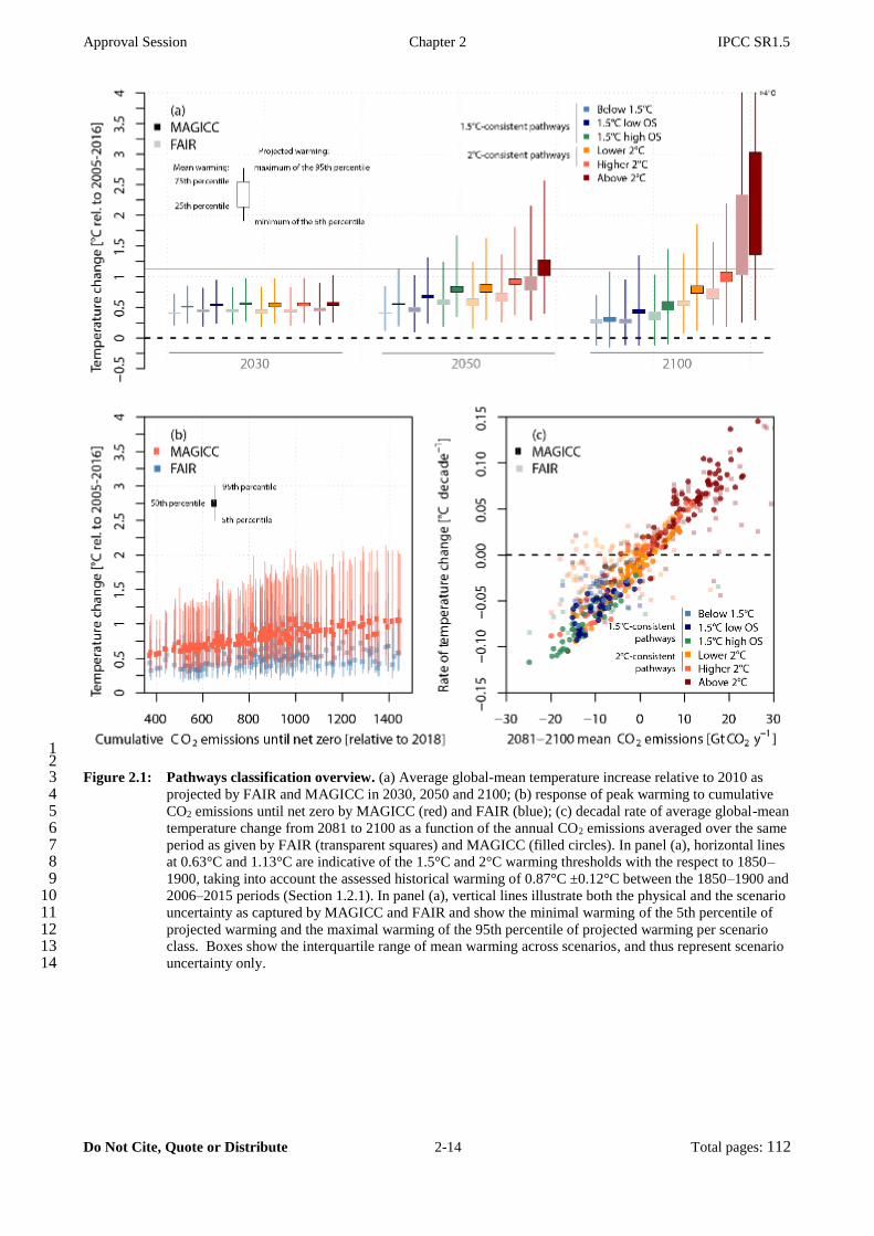
1 2 Figure 2.1: Pathways classification overview. (a) Average global-mean temperature increase relative to 2010 as 3
projected by FAIR and MAGICC in 2030, 2050 and 2100; (b) response of peak warming to cumulative 4 CO2 emissions until net zero by MAGICC (red) and FAIR (blue); (c) decadal rate of average global-mean 5 temperature change from 2081 to 2100 as a function of the annual CO2 emissions averaged over the same 6 period as given by FAIR (transparent squares) and MAGICC (filled circles). In panel (a), horizontal lines 7 at 0.63°C and 1.13°C are indicative of the 1.5°C and 2°C warming thresholds with the respect to 1850–8 1900, taking into account the assessed historical warming of 0.87°C ±0.12°C between the 1850–1900 and 9 2006–2015 periods (Section 1.2.1). In panel (a), vertical lines illustrate both the physical and the scenario 10 uncertainty as captured by MAGICC and FAIR and show the minimal warming of the 5th percentile of 11 projected warming and the maximal warming of the 95th percentile of projected warming per scenario 12 class. Boxes show the interquartile range of mean warming across scenarios, and thus represent scenario 13 uncertainty only.14
Final Government Draft Chapter 2 IPCC SR1.5
Do Not Cite, Quote or Distribute 2-15 Total pages: 112
Geophysical uncertainties: non-CO2 forcing agents 1
2
Impacts of non-CO2 climate forcers on temperature outcomes are particularly important when evaluating 3
stringent mitigation pathways (Weyant et al., 2006; Shindell et al., 2012; Rogelj et al., 2014b, 2015a; Samset 4
et al., 2018). However, many uncertainties affect the role of non-CO2 climate forcers in stringent mitigation 5
pathways. 6
7
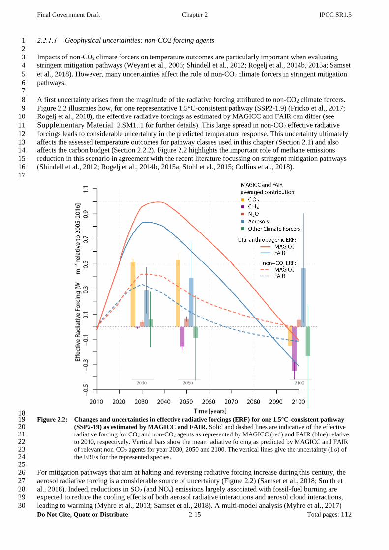
A first uncertainty arises from the magnitude of the radiative forcing attributed to non-CO2 climate forcers. 8
Figure 2.2 illustrates how, for one representative 1.5°C-consistent pathway (SSP2-1.9) (Fricko et al., 2017; 9
Rogelj et al., 2018), the effective radiative forcings as estimated by MAGICC and FAIR can differ (see 10
Supplementary Material 2.SM1..1 for further details). This large spread in non-CO2 effective radiative 11
forcings leads to considerable uncertainty in the predicted temperature response. This uncertainty ultimately 12
affects the assessed temperature outcomes for pathway classes used in this chapter (Section 2.1) and also 13
affects the carbon budget (Section 2.2.2). Figure 2.2 highlights the important role of methane emissions 14
reduction in this scenario in agreement with the recent literature focussing on stringent mitigation pathways 15
(Shindell et al., 2012; Rogelj et al., 2014b, 2015a; Stohl et al., 2015; Collins et al., 2018). 16
17
18 Figure 2.2: Changes and uncertainties in effective radiative forcings (ERF) for one 1.5°C-consistent pathway 19
(SSP2-19) as estimated by MAGICC and FAIR. Solid and dashed lines are indicative of the effective 20 radiative forcing for CO2 and non-CO2 agents as represented by MAGICC (red) and FAIR (blue) relative 21 to 2010, respectively. Vertical bars show the mean radiative forcing as predicted by MAGICC and FAIR 22 of relevant non-CO2 agents for year 2030, 2050 and 2100. The vertical lines give the uncertainty (1σ) of 23 the ERFs for the represented species. 24
25 For mitigation pathways that aim at halting and reversing radiative forcing increase during this century, the 26
aerosol radiative forcing is a considerable source of uncertainty (Figure 2.2) (Samset et al., 2018; Smith et 27
al., 2018). Indeed, reductions in SO2 (and NOx) emissions largely associated with fossil-fuel burning are 28
expected to reduce the cooling effects of both aerosol radiative interactions and aerosol cloud interactions, 29
leading to warming (Myhre et al., 2013; Samset et al., 2018). A multi-model analysis (Myhre et al., 2017) 30
Final Government Draft Chapter 2 IPCC SR1.5
Do Not Cite, Quote or Distribute 2-16 Total pages: 112
and a study based on observational constraints (Malavelle et al., 2017) largely support the AR5 best estimate 1
and uncertainty range of aerosol forcing. The partitioning of total aerosol radiative forcing between aerosol 2
precursor emissions is important (Ghan et al., 2013; Jones et al., 2018; Smith et al., 2018) as this affects the 3
estimate of the mitigation potential from different sectors that have aerosol precursor emission sources. The 4
total aerosol effective radiative forcing change in stringent mitigation pathways is expected to be dominated 5
by the effects from the phase-out of SO2, although the magnitude of this aerosol-warming effect depends on 6
how much of the present-day aerosol cooling is attributable to SO2, particularly the cooling associated with 7
aerosol-cloud interaction (Figure 2.2). Regional differences in the linearity of aerosol-cloud interaction 8
(Carslaw et al., 2013; Kretzschmar et al., 2017) make it difficult to separate the role of individual precursors. 9
Precursors that are not fully mitigated will continue to affect the Earth system. If, for example, the role of 10
nitrate aerosol cooling is at the strongest end of the assessed IPCC AR5 uncertainty range, future 11
temperature increases may be more modest if ammonia emissions continue to rise (Hauglustaine et al., 12
2014). 13
14
Figure 2.2 shows that there are substantial differences in the evolution of estimated effective radiative 15
forcing of non-CO2 forcers between MAGICC and FAIR. These forcing differences result in MAGICC 16
simulating a larger warming trend in the near term compared to both the FAIR model and the recent 17
observed trends of 0.2°C per decade reported in Chapter 1 (Figure 2.1, Supplementary Material 2.SM.1.1, 18
Section 1.2.1.3). The aerosol effective forcing is stronger in MAGICC compared to either FAIR or the AR5 19
best estimate, though it is still well within the AR5 uncertainty range (Supplementary 20
Material 2.SM.1.1.1). A recent revision (Etminan et al., 2016) increases the methane forcing by 25%. This 21
revision is used in the FAIR but not in the AR5 setup of MAGICC that is applied here. Other structural 22
differences exist in how the two models relate emissions to concentrations that contribute to differences in 23
forcing (see Supplementary Material 2.SM.1.1.1). 24
25
Non-CO2 climate forcers exhibit a greater geographical variation in radiative forcings than CO2, which lead 26
to important uncertainties in the temperature response (Myhre et al., 2013). This uncertainty increases the 27
relative uncertainty of the temperature pathways associated with low emission scenarios compared to high 28
emission scenarios (Clarke et al., 2014). It is also important to note that geographical patterns of temperature 29
change and other climate responses, especially those related to precipitation, depend significantly on the 30
forcing mechanism (Myhre et al., 2013; Shindell et al., 2015; Marvel et al., 2016; Samset et al., 2016) (see 31
also Section 3.6.2.2). 32
33
34
Geophysical uncertainties: climate and Earth-system feedbacks 35
36
Climate sensitivity uncertainty impacts future projections as well as carbon-budget estimates (Schneider et 37
al., 2017). AR5 assessed the equilibrium climate sensitivity (ECS) to be likely in the 1.5–4.5°C range, 38
extremely unlikely less than 1°C and very unlikely greater than 6°C. The lower bound of this estimate is 39
lower than the range of CMIP5 models (Collins et al., 2013). The evidence for the 1.5°C lower bound on 40
ECS in AR5 was based on analysis of energy-budget changes over the historical period. Work since AR5 has 41
suggested that the climate sensitivity inferred from such changes has been lower than the 2xCO2 climate 42
sensitivity for known reasons (Forster, 2016; Gregory and Andrews, 2016; Rugenstein et al., 2016; Armour, 43
2017; Ceppi and Gregory, 2017; Knutti et al., 2017; Proistosescu and Huybers, 2017). Both a revised 44
interpretation of historical estimates and other lines of evidence based on analysis of climate models with the 45
best representation of today’s climate (Sherwood et al., 2014; Zhai et al., 2015; Tan et al., 2016; Brown and 46
Caldeira, 2017; Knutti et al., 2017) suggest that the lower bound of ECS could be revised upwards which 47
would decrease the chances of limiting warming below 1.5°C in assessed pathways. However, such a 48
reassessment has been challenged (Lewis and Curry, 2018), albeit from a single line of evidence. 49
Nevertheless, it is premature to make a major revision to the lower bound. The evidence for a possible 50
revision of the upper bound on ECS is less clear with cases argued from different lines of evidence for both 51
decreasing (Lewis and Curry, 2015, 2018; Cox et al., 2018) and increasing (Brown and Caldeira, 2017) the 52
bound presented in the literature. The tools used in this chapter employ ECS ranges consistent with the AR5 53
assessment. The MAGICC ECS distribution has not been selected to explicitly reflect this but is nevertheless 54
consistent (Rogelj et al., 2014a). The FAIR model used here to estimate carbon budgets explicitly constructs 55
log-normal distributions of ECS and transient climate response based on a multi parameter fit to the AR5 56
Final Government Draft Chapter 2 IPCC SR1.5
Do Not Cite, Quote or Distribute 2-17 Total pages: 112
assessed ranges of climate sensitivity and individual historic effective radiative forcings (Smith et al., 2018) 1
(Supplementary Material 2.SM.1.1.1). 2
3
Several feedbacks of the Earth system, involving the carbon cycle, non-CO2 GHGs and/or aerosols, may also 4
impact the future dynamics of the coupled carbon-climate system’s response to anthropogenic emissions. 5
These feedbacks are caused by the effects of nutrient limitation (Duce et al., 2008; Mahowald et al., 2017), 6
ozone exposure (de Vries et al., 2017), fire emissions (Narayan et al., 2007) and changes associated with 7
natural aerosols (Cadule et al., 2009; Scott et al., 2017). Among these Earth-system feedbacks, the 8
importance of the permafrost feedback’s influence has been highlighted in recent studies. Combined 9
evidence from both models (MacDougall et al., 2015; Burke et al., 2017; Lowe and Bernie, 2018) and field 10
studies (like Schädel et al., 2014; Schuur et al., 2015) shows high agreement that permafrost thawing will 11
release both CO2 and CH4 as the Earth warms, amplifying global warming. This thawing could also release 12
N2O (Voigt et al., 2017a, 2017b). Field, laboratory and modelling studies estimate that the vulnerable 13
fraction in permafrost is about 5–15% of the permafrost soil carbon (~5300–5600 GtCO2 in Schuur et al., 14
2015) and that carbon emissions are expected to occur beyond 2100 because of system inertia and the large 15
proportion of slowly decomposing carbon in permafrost (Schädel et al., 2014). Published model studies 16
suggest that a large part of the carbon release to the atmosphere is in the form of CO2 (Schädel et al., 2016), 17
while the amount of CH4 released by permafrost thawing is estimated to be much smaller than that CO2. 18
Cumulative CH4 release by 2100 under RCP2.6 ranges from 0.13 to 0.45 Gt of methane (Burke et al., 2012; 19
Schneider von Deimling et al., 2012, 2015) with fluxes being the highest in the middle of the century 20
because of maximum thermokarst lake extent by mid-century (Schneider von Deimling et al., 2015). 21
22
The reduced complexity climate models employed in this assessment do not take into account permafrost or 23
non-CO2 Earth-system feedbacks, although the MAGICC model has a permafrost module that can be 24
enabled. Taking the current climate and Earth-system feedbacks understanding together, there is a possibility 25
that these models would underestimate the longer-term future temperature response to stringent emission 26
pathways (Section 2.2.2). 27
28
29
2.2.2 The remaining 1.5°C carbon budget 30
31
Carbon budget estimates 32
33
Since the AR5, several approaches have been proposed to estimate carbon budgets compatible with 1.5°C or 34
2°C. Most of these approaches indirectly rely on the approximate linear relationship between peak global-35
mean temperature and cumulative emissions of carbon (the transient climate response to cumulative 36
emissions of carbon, TCRE (Collins et al., 2013; Friedlingstein et al., 2014a; Rogelj et al., 2016b) whereas 37
others base their estimates on equilibrium climate sensitivity (Schneider et al., 2017). The AR5 employed 38
two approaches to determine carbon budgets. Working Group I (WGI) computed carbon budgets from 2011 39
onwards for various levels of warming relative to the 1861–1880 period using RCP8.5 (Meinshausen et al., 40
2011b; Stocker et al., 2013) whereas WGIII estimated their budgets from a set of available pathways that 41
were assessed to have a >50% probability to exceed 1.5°C by mid-century, and return to 1.5°C or below in 42
2100 with greater than 66% probability (Clarke et al., 2014). These differences made AR5 WGI and WGIII 43
carbon budgets difficult to compare as they are calculated over different time periods, derived from a 44
different sets of multi-gas and aerosol emission scenarios and use different concepts of carbon budgets 45
(exceedance for WGI, avoidance for WGIII) (Rogelj et al., 2016b; Matthews et al., 2017). 46
47
Carbon budgets can be derived from CO2-only experiments as well as from multi-gas and aerosol scenarios. 48
Some published estimates of carbon budgets compatible with 1.5°C or 2°C refer to budgets for CO2-induced 49
warming only, and hence do not take into account the contribution of non-CO2 climate forcers (Allen et al., 50
2009; Matthews et al., 2009; Zickfeld et al., 2009; IPCC, 2013a). However, because the projected changes in 51
non-CO2 climate forcers tend to amplify future warming, CO2-only carbon budgets overestimate the total net 52
cumulative carbon emissions compatible with 1.5°C or 2°C (Friedlingstein et al., 2014a; Rogelj et al., 2016b; 53
Matthews et al., 2017; Mengis et al., 2018; Tokarska et al., 2018). 54
55
Since the AR5, many estimates of the remaining carbon budget for 1.5°C have been published 56
(Friedlingstein et al., 2014a; MacDougall et al., 2015; Peters, 2016; Rogelj et al., 2016b; Matthews et al., 57

Final Government Draft Chapter 2 IPCC SR1.5
Do Not Cite, Quote or Distribute 2-18 Total pages: 112
2017; Millar et al., 2017; Goodwin et al., 2018b; Kriegler et al., 2018a; Lowe and Bernie, 2018; Mengis et 1
al., 2018; Millar and Friedlingstein, 2018; Rogelj et al., 2018; Schurer et al., 2018; Séférian et al., 2018; 2
Tokarska et al., 2018; Tokarska and Gillett, 2018). These estimates cover a wide range as a result of 3
differences in the models used, and of methodological choices, as well as physical uncertainties. Some 4
estimates are exclusively model-based while others are based on observations or on a combination of both. 5
Remaining carbon budgets limiting warming below 1.5°C or 2°C that are derived from Earth-system models 6
of intermediate complexity (MacDougall et al., 2015; Goodwin et al., 2018a), IAMs (Luderer et al., 2018; 7
Rogelj et al., 2018), or based on Earth-system model results (Lowe and Bernie, 2018; Séférian et al., 2018; 8
Tokarska and Gillett, 2018) give remaining carbon budgets of the same order of magnitude than the IPCC 9
AR5 Synthesis Report (SYR) estimates (IPCC, 2014a). This is unsurprising as similar sets of models were 10
used for the AR5 (IPCC, 2013b). The range of variation across models stems mainly from either the 11
inclusion or exclusion of specific Earth-system feedbacks (MacDougall et al., 2015; Burke et al., 2017; 12
Lowe and Bernie, 2018) or different budget definitions (Rogelj et al., 2018). 13
14
In contrast to the model-only estimates discussed above and employed in the AR5, this report additionally 15
uses observations to inform its evaluation of the remaining carbon budget. Table 2.2 shows that the assessed 16
range of remaining carbon budgets consistent with 1.5°C or 2°C is larger than the AR5 SYR estimate and is 17
part way towards estimates constrained by recent observations (Millar et al., 2017; Goodwin et al., 2018a; 18
Tokarska and Gillett, 2018). Figure 2.3 illustrates that the change since AR5 is, in very large part, due to the 19
application of a more recent observed baseline to the historic temperature change and cumulative emissions; 20
here adopting the baseline period of 2006-2015 (see Section 1.2.1). AR5 SYR Figures SPM.10 and 2.3 21
already illustrated the discrepancy between models and observations, but did not apply this as a correction to 22
the carbon budget because they were being used to illustrate the overall linear relationship between warming 23
and cumulative carbon emissions in the CMIP5 models since 1870, and were not specifically designed to 24
quantify residual carbon budgets relative to the present for ambitious temperature goals. The AR5 SYR 25
estimate was also dependent on a subset of Earth-system models illustrated in Figure 2.3 of this report. 26
Although, as outlined below and in Table 2.2, considerably uncertainties remain, there is high agreement 27
across various lines of evidence assessed in this report that the remaining carbon budget for 1.5°C or 2°C 28
would be larger than the estimates at the time of the AR5. However, the overall remaining budget for 2100 is 29
assessed to be smaller than that derived from the recent observational-informed estimates, as Earth-system 30
feedbacks such as permafrost thawing reduce the budget applicable to centennial scales (see Section 2.2.2.2). 31
32
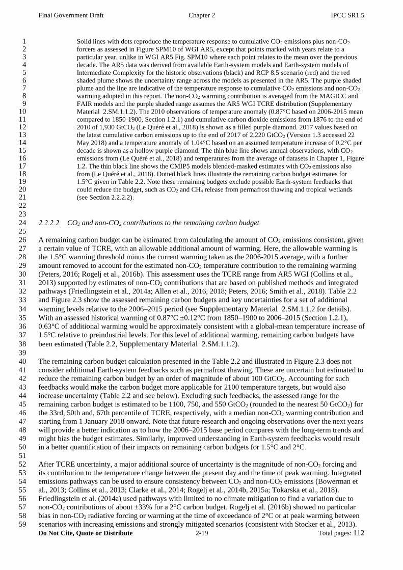
33 Figure 2.3: Temperature changes from 1850-1900 versus cumulative CO2 emissions since 1st January 1876. 34
Final Government Draft Chapter 2 IPCC SR1.5
Do Not Cite, Quote or Distribute 2-19 Total pages: 112
Solid lines with dots reproduce the temperature response to cumulative CO2 emissions plus non-CO2 1 forcers as assessed in Figure SPM10 of WGI AR5, except that points marked with years relate to a 2 particular year, unlike in WGI AR5 Fig. SPM10 where each point relates to the mean over the previous 3 decade. The AR5 data was derived from available Earth-system models and Earth-system models of 4 Intermediate Complexity for the historic observations (black) and RCP 8.5 scenario (red) and the red 5 shaded plume shows the uncertainty range across the models as presented in the AR5. The purple shaded 6 plume and the line are indicative of the temperature response to cumulative CO2 emissions and non-CO2 7 warming adopted in this report. The non-CO2 warming contribution is averaged from the MAGICC and 8 FAIR models and the purple shaded range assumes the AR5 WGI TCRE distribution (Supplementary 9 Material 2.SM.1.1.2). The 2010 observations of temperature anomaly (0.87°C based on 2006-2015 mean 10 compared to 1850-1900, Section 1.2.1) and cumulative carbon dioxide emissions from 1876 to the end of 11 2010 of 1,930 GtCO2 (Le Quéré et al., 2018) is shown as a filled purple diamond. 2017 values based on 12 the latest cumulative carbon emissions up to the end of 2017 of 2,220 GtCO2 (Version 1.3 accessed 22 13 May 2018) and a temperature anomaly of 1.04°C based on an assumed temperature increase of 0.2°C per 14 decade is shown as a hollow purple diamond. The thin blue line shows annual observations, with CO2 15 emissions from (Le Quéré et al., 2018) and temperatures from the average of datasets in Chapter 1, Figure 16 1.2. The thin black line shows the CMIP5 models blended-masked estimates with CO2 emissions also 17 from (Le Quéré et al., 2018). Dotted black lines illustrate the remaining carbon budget estimates for 18 1.5°C given in Table 2.2. Note these remaining budgets exclude possible Earth-system feedbacks that 19 could reduce the budget, such as CO2 and CH4 release from permafrost thawing and tropical wetlands 20 (see Section 2.2.2.2). 21
22
23
CO2 and non-CO2 contributions to the remaining carbon budget 24
25
A remaining carbon budget can be estimated from calculating the amount of CO2 emissions consistent, given 26
a certain value of TCRE, with an allowable additional amount of warming. Here, the allowable warming is 27
the 1.5°C warming threshold minus the current warming taken as the 2006-2015 average, with a further 28
amount removed to account for the estimated non-CO2 temperature contribution to the remaining warming 29
(Peters, 2016; Rogelj et al., 2016b). This assessment uses the TCRE range from AR5 WGI (Collins et al., 30
2013) supported by estimates of non-CO2 contributions that are based on published methods and integrated 31
pathways (Friedlingstein et al., 2014a; Allen et al., 2016, 2018; Peters, 2016; Smith et al., 2018). Table 2.2 32
and Figure 2.3 show the assessed remaining carbon budgets and key uncertainties for a set of additional 33
warming levels relative to the 2006–2015 period (see Supplementary Material 2.SM.1.1.2 for details). 34
With an assessed historical warming of 0.87°C ±0.12°C from 1850–1900 to 2006–2015 (Section 1.2.1), 35
0.63°C of additional warming would be approximately consistent with a global-mean temperature increase of 36
1.5°C relative to preindustrial levels. For this level of additional warming, remaining carbon budgets have 37
been estimated (Table 2.2, Supplementary Material 2.SM.1.1.2). 38
39
The remaining carbon budget calculation presented in the Table 2.2 and illustrated in Figure 2.3 does not 40
consider additional Earth-system feedbacks such as permafrost thawing. These are uncertain but estimated to 41
reduce the remaining carbon budget by an order of magnitude of about 100 GtCO2. Accounting for such 42
feedbacks would make the carbon budget more applicable for 2100 temperature targets, but would also 43
increase uncertainty (Table 2.2 and see below). Excluding such feedbacks, the assessed range for the 44
remaining carbon budget is estimated to be 1100, 750, and 550 GtCO2 (rounded to the nearest 50 GtCO2) for 45
the 33rd, 50th and, 67th percentile of TCRE, respectively, with a median non-CO2 warming contribution and 46
starting from 1 January 2018 onward. Note that future research and ongoing observations over the next years 47
will provide a better indication as to how the 2006–2015 base period compares with the long-term trends and 48
might bias the budget estimates. Similarly, improved understanding in Earth-system feedbacks would result 49
in a better quantification of their impacts on remaining carbon budgets for 1.5°C and 2°C. 50
51
After TCRE uncertainty, a major additional source of uncertainty is the magnitude of non-CO2 forcing and 52
its contribution to the temperature change between the present day and the time of peak warming. Integrated 53
emissions pathways can be used to ensure consistency between CO2 and non-CO2 emissions (Bowerman et 54
al., 2013; Collins et al., 2013; Clarke et al., 2014; Rogelj et al., 2014b, 2015a; Tokarska et al., 2018). 55
Friedlingstein et al. (2014a) used pathways with limited to no climate mitigation to find a variation due to 56
non-CO2 contributions of about ±33% for a 2°C carbon budget. Rogelj et al. (2016b) showed no particular 57
bias in non-CO2 radiative forcing or warming at the time of exceedance of 2°C or at peak warming between 58
scenarios with increasing emissions and strongly mitigated scenarios (consistent with Stocker et al., 2013). 59

Final Government Draft Chapter 2 IPCC SR1.5
Do Not Cite, Quote or Distribute 2-20 Total pages: 112
However, clear differences of the non-CO2 warming contribution at the time of deriving a 2°C-consistent 1
carbon budget were reported for the four RCPs. Although the spread in non-CO2 forcing across scenarios can 2
be smaller in absolute terms at lower levels of cumulative emissions, it can be larger in relative terms 3
compared to the remaining carbon budget (Stocker et al., 2013; Friedlingstein et al., 2014a; Rogelj et al., 4
2016b). Tokarska and Gillett (2018) find no statistically significant differences in 1.5°C-consistent 5
cumulative emissions budgets when calculated for different RCPs from consistent sets of CMIP5 6
simulations. 7
8
The mitigation pathways assessed in this report indicate that emissions of non-CO2 forcers contribute an 9
average additional warming of around 0.15°C relative to 2006–2015 at the time of net zero CO2 emissions, 10
reducing the remaining carbon budget by roughly 320 GtCO2. This arises from a weakening of aerosol 11
cooling and continued emissions of non-CO2 GHGs (Sections 2.2.1, 2.3.3). This non-CO2 contribution at the 12
time of net zero CO2 emissions varies by about ±0.1°C across scenarios resulting in a carbon budget 13
uncertainty of about ±250 GtCO2 and takes into account marked reductions in methane emissions (Section 14
2.3.3). In case these would not be achieved, remaining carbon budgets are further reduced. Uncertainties in 15
the non-CO2 forcing and temperature response are asymmetric and can influence the remaining carbon 16
budget by -400 to +200 GtCO2 with the uncertainty in aerosol radiative forcing being the largest contributing 17
factor (Table 2.2). The MAGICC and FAIR models in their respective parameter setups and model versions 18
used to assess the non-CO2 warming contribution give noticeable different non-CO2 effective radiative 19
forcing and warming for the same scenarios while both being within plausible ranges of future response (Fig. 20
2.2 and Supplementary Material 2.SM.1.1, 2.SM.1.2). For this assessment, it is premature to assess the 21
accuracy of their results, so it is assumed that both are equally representative of possible futures. Their non-22
CO2 warming estimates are therefore averaged for the carbon budget assessment and their differences used to 23
guide the uncertainty assessment of the role of non-CO2 forcers. Nevertheless, the findings are robust enough 24
to give high confidence that the changing emissions non-CO2 forcers (particularly the reduction in cooling 25
aerosol precursors) cause additional near-term warming and reduce the remaining carbon budget compared 26
to the CO2 only budget. 27
28
TCRE uncertainty directly impacts carbon budget estimates (Peters, 2016; Matthews et al., 2017; Millar and 29
Friedlingstein, 2018). Based on multiple lines of evidence, AR5 WGI assessed a likely range for TCRE of 30
0.2–0.7°C per 1000 GtCO2 (Collins et al., 2013). The TCRE of the CMIP5 Earth-system models ranges from 31
0.23 to 0.66°C per 1000 GtCO2 (Gillett et al., 2013). At the same time, studies using observational 32
constraints find best estimates of TCRE of 0.35–0.41°C per 1000 GtCO2 (Matthews et al., 2009; Gillett et 33
al., 2013; Tachiiri et al., 2015; Millar and Friedlingstein, 2018). This assessment continues to use the 34
assessed AR5 TCRE range under the working assumption that TCRE is normally distributed (Stocker et al., 35
2013). Observation-based estimates have reported log-normal distributions of TCRE (Millar and 36
Friedlingstein, 2018). Assuming a log-normal instead of normal distribution of the assessed AR5 TCRE 37
range would result in about a 200 GtCO2 increase for the median budget estimates but only about half at the 38
67th percentile, while historical temperature uncertainty and uncertainty in recent emissions contribute ±150 39
and ±50 GtCO2 to the uncertainty, respectively (Table 2.2). 40
41
Calculating carbon budgets from the TCRE requires the assumption that the instantaneous warming in 42
response to cumulative CO2 emissions equals the long-term warming or, equivalently, that the residual 43
warming after CO2 emissions cease is negligible. The magnitude of this residual warming, referred to as the 44
zero-emission commitment, ranges from slightly negative (i.e., a slight cooling) to slightly positive for CO2 45
emissions up to present-day (Section 1.2.4) (Lowe et al., 2009; Frölicher and Joos, 2010; Gillett et al., 2011; 46
Matthews and Zickfeld, 2012). The delayed temperature change from a pulse CO2 emission introduces 47
uncertainties in emission budgets, which have not been quantified in the literature for budgets consistent with 48
limiting warming to 1.5°C. As a consequence, this uncertainty does not affect our carbon budget estimates 49
directly but it is included as an additional factor in the assessed Earth-system feedback uncertainty (as 50
detailed below) of roughly 100 GtCO2 on decadal timescales presented in Table 2.2. 51
52
Remaining carbon budgets are further influenced by Earth-system feedbacks not accounted for in CMIP5 53
models, such as the permafrost carbon feedback (Friedlingstein et al., 2014b; MacDougall et al., 2015; Burke 54
et al., 2017; Lowe and Bernie, 2018), and their influence on the TCRE. Lowe and Bernie (2018) used a 55
simple climate sensitivity scaling approach to estimate that Earth-system feedbacks (such as CO2 released by 56
permafrost thawing or methane released by wetlands) could reduce carbon budgets for 1.5°C and 2°C by 57
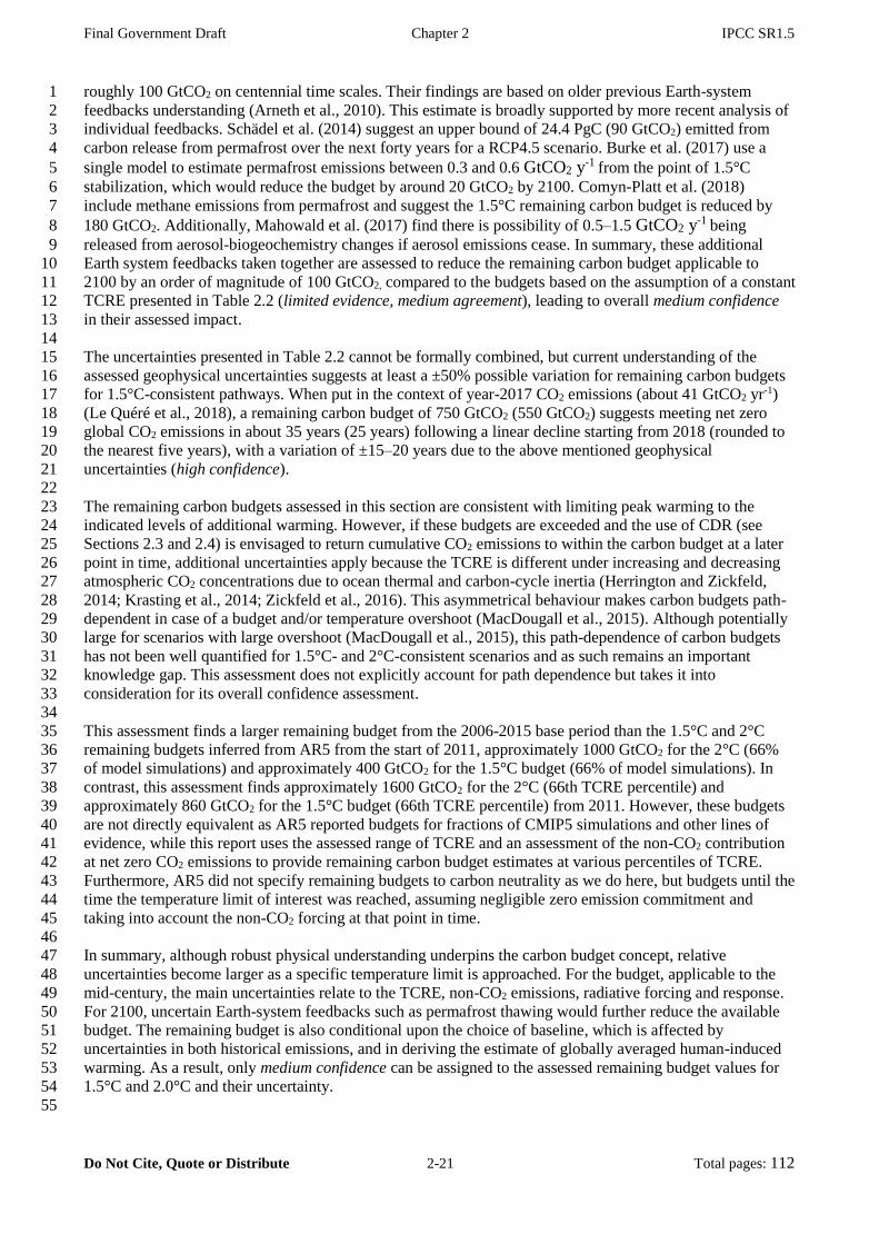
Final Government Draft Chapter 2 IPCC SR1.5
Do Not Cite, Quote or Distribute 2-21 Total pages: 112
roughly 100 GtCO2 on centennial time scales. Their findings are based on older previous Earth-system 1
feedbacks understanding (Arneth et al., 2010). This estimate is broadly supported by more recent analysis of 2
individual feedbacks. Schädel et al. (2014) suggest an upper bound of 24.4 PgC (90 GtCO2) emitted from 3
carbon release from permafrost over the next forty years for a RCP4.5 scenario. Burke et al. (2017) use a 4
single model to estimate permafrost emissions between 0.3 and 0.6 GtCO2 y-1 from the point of 1.5°C 5
stabilization, which would reduce the budget by around 20 GtCO2 by 2100. Comyn-Platt et al. (2018) 6
include methane emissions from permafrost and suggest the 1.5°C remaining carbon budget is reduced by 7
180 GtCO2. Additionally, Mahowald et al. (2017) find there is possibility of 0.5–1.5 GtCO2 y-1 being 8
released from aerosol-biogeochemistry changes if aerosol emissions cease. In summary, these additional 9
Earth system feedbacks taken together are assessed to reduce the remaining carbon budget applicable to 10
2100 by an order of magnitude of 100 GtCO2, compared to the budgets based on the assumption of a constant 11
TCRE presented in Table 2.2 (limited evidence, medium agreement), leading to overall medium confidence 12
in their assessed impact. 13
14
The uncertainties presented in Table 2.2 cannot be formally combined, but current understanding of the 15
assessed geophysical uncertainties suggests at least a ±50% possible variation for remaining carbon budgets 16
for 1.5°C-consistent pathways. When put in the context of year-2017 CO2 emissions (about 41 GtCO2 yr-1) 17
(Le Quéré et al., 2018), a remaining carbon budget of 750 GtCO2 (550 GtCO2) suggests meeting net zero 18
global CO2 emissions in about 35 years (25 years) following a linear decline starting from 2018 (rounded to 19
the nearest five years), with a variation of ±15–20 years due to the above mentioned geophysical 20
uncertainties (high confidence). 21
22
The remaining carbon budgets assessed in this section are consistent with limiting peak warming to the 23
indicated levels of additional warming. However, if these budgets are exceeded and the use of CDR (see 24
Sections 2.3 and 2.4) is envisaged to return cumulative CO2 emissions to within the carbon budget at a later 25
point in time, additional uncertainties apply because the TCRE is different under increasing and decreasing 26
atmospheric CO2 concentrations due to ocean thermal and carbon-cycle inertia (Herrington and Zickfeld, 27
2014; Krasting et al., 2014; Zickfeld et al., 2016). This asymmetrical behaviour makes carbon budgets path-28
dependent in case of a budget and/or temperature overshoot (MacDougall et al., 2015). Although potentially 29
large for scenarios with large overshoot (MacDougall et al., 2015), this path-dependence of carbon budgets 30
has not been well quantified for 1.5°C- and 2°C-consistent scenarios and as such remains an important 31
knowledge gap. This assessment does not explicitly account for path dependence but takes it into 32
consideration for its overall confidence assessment. 33
34
This assessment finds a larger remaining budget from the 2006-2015 base period than the 1.5°C and 2°C 35
remaining budgets inferred from AR5 from the start of 2011, approximately 1000 GtCO2 for the 2°C (66% 36
of model simulations) and approximately 400 GtCO2 for the 1.5°C budget (66% of model simulations). In 37
contrast, this assessment finds approximately 1600 GtCO2 for the 2°C (66th TCRE percentile) and 38
approximately 860 GtCO2 for the 1.5°C budget (66th TCRE percentile) from 2011. However, these budgets 39
are not directly equivalent as AR5 reported budgets for fractions of CMIP5 simulations and other lines of 40
evidence, while this report uses the assessed range of TCRE and an assessment of the non-CO2 contribution 41
at net zero CO2 emissions to provide remaining carbon budget estimates at various percentiles of TCRE. 42
Furthermore, AR5 did not specify remaining budgets to carbon neutrality as we do here, but budgets until the 43
time the temperature limit of interest was reached, assuming negligible zero emission commitment and 44
taking into account the non-CO2 forcing at that point in time. 45
46
In summary, although robust physical understanding underpins the carbon budget concept, relative 47
uncertainties become larger as a specific temperature limit is approached. For the budget, applicable to the 48
mid-century, the main uncertainties relate to the TCRE, non-CO2 emissions, radiative forcing and response. 49
For 2100, uncertain Earth-system feedbacks such as permafrost thawing would further reduce the available 50
budget. The remaining budget is also conditional upon the choice of baseline, which is affected by 51
uncertainties in both historical emissions, and in deriving the estimate of globally averaged human-induced 52
warming. As a result, only medium confidence can be assigned to the assessed remaining budget values for 53
1.5°C and 2.0°C and their uncertainty. 54
55
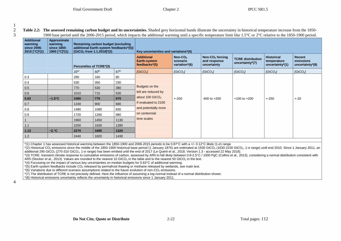
Final Government Draft Chapter 2 IPCC SR1.5
Do Not Cite, Quote or Distribute 2-22 Total pages: 112
1 Table 2.2: The assessed remaining carbon budget and its uncertainties. Shaded grey horizontal bands illustrate the uncertainty in historical temperature increase from the 1850-2
1900 base period until the 2006-2015 period, which impacts the additional warming until a specific temperature limit like 1.5°C or 2°C relative to the 1850-1900 period. 3 Additional warming since 2006-2015 [°C]*(1)
Approximate warming since 1850-1900 [°C]*(1)
Remaining carbon budget (excluding additional Earth-system feedbacks*(5)) [GtCO2 from 1.1.2018]*(2) Key uncertainties and variations*(4)
Percentiles of TCRE*(3)
Additional Earth-system feedbacks*(5)
Non-CO2 scenario variation*(6)
Non-CO2 forcing and response uncertainty
TCRE distribution uncertainty*(7)
Historical temperature uncertainty*(1)
Recent emissions uncertainty*(8)
33rd 50th 67th [GtCO2] [GtCO2] [GtCO2] [GtCO2] [GtCO2] [GtCO2]
0.3 290 160 80
0.4 530 350 230
0.5 770 530 380 Budgets on the
0.6 1010 710 530 left are reduced by
0.63 ~1.5°C 1080 770 570 about 100 GtCO2 +-250 -400 to +200 +100 to +200 +-250 +-20
0.7 1240 900 680 If evaluated to 2100
0.8 1480 1080 830 and potentially more
0.9 1720 1260 980 on centennial
1 1960 1450 1130 time scales
1.1 2200 1630 1280
1.13 ~2.°C 2270 1690 1320
1.2 2440 1820 1430
*(1) Chapter 1 has assessed historical warming between the 1850-1900 and 2006-2015 periods to be 0.87°C with a +/- 0.12°C likely (1-σ) range *(2) Historical CO2 emissions since the middle of the 1850-1900 historical base period (1 January 1876) are estimated at 1930 GtCO2 (1630-2230 GtCO2, 1-σ range) until end 2010. Since 1 January 2011, an additional 290 GtCO2 (270-310 GtCO2, 1-σ range) has been emitted until the end of 2017 (Le Quéré et al., 2018, Version 1.3 - accessed 22 May 2018). *(3) TCRE: transient climate response to cumulative emissions of carbon, assessed by AR5 to fall likely between 0.8-2.5°C / 1000 PgC (Collins et al., 2013), considering a normal distribution consistent with AR5 (Stocker et al., 2013). Values are rounded to the nearest 10 GtCO2 in the table and to the nearest 50 GtCO2 in the text. *(4) Focussing on the impact of various key uncertainties on median budgets for 0.63°C of additional warming. *(5) Earth system feedbacks include CO2 released by permafrost thawing or methane released by wetlands, see main text. *(6) Variations due to different scenario assumptions related to the future evolution of non-CO2 emissions. *(7) The distribution of TCRE is not precisely defined. Here the influence of assuming a log-normal instead of a normal distribution shown. *(8) Historical emissions uncertainty reflects the uncertainty in historical emissions since 1 January 2011.
4

Final Government Draft Chapter 2 IPCC SR1.5
Do Not Cite, Quote or Distribute 2-23 Total pages: 112
2.3 Overview of 1.5°C mitigation pathways 1
2
Limiting global mean temperature increase at any level requires global CO2 emissions to become net zero at 3
some point in the future (Zickfeld et al., 2009; Collins et al., 2013). At the same time, limiting the residual 4
warming of short-lived non-CO2 emissions, can be achieved by reducing their annual emissions as far as 5
possible (Section 2.2, Cross-Chapter Box 2 in Chapter 1). This will require large-scale transformations of the 6
global energy-agriculture-land-economy system, affecting the way in which energy is produced, agricultural 7
systems are organised, and food, energy and materials are consumed (Clarke et al., 2014). This section 8
assesses key properties of pathways consistent with limiting global mean temperature to 1.5°C relative to 9
pre-industrial levels, including their underlying assumptions and variations. 10
11
Since the AR5, an extensive body of literature has appeared on integrated pathways consistent with 1.5°C ( 12
Rogelj et al., 2015b; Akimoto et al., 2017; Liu et al., 2017; Löffler et al., 2017; Marcucci et al., 2017; Su et 13
al., 2017; Bauer et al., 2018; Bertram et al., 2018; Grubler et al., 2018; Kriegler et al., 2018b; Luderer et al., 14
2018; Rogelj et al., 2018; Strefler et al., 2018a; van Vuuren et al., 2018; Vrontisi et al., 2018; Zhang et al., 15
2018) (Section 2.1). These pathways have global coverage and represent all GHG-emitting sectors and their 16
interactions. Such integrated pathways allow the exploration of the whole-system transformation, and hence 17
provide the context in which the detailed sectorial transformations assessed in Section 2.4 of this chapter are 18
taking place. 19
20
The overwhelming majority of published integrated pathways have been developed by global IAMs that 21
represent key societal systems and their interactions, like the energy system, agriculture and land use, and the 22
economy (see Section 6.2 in Clarke et al., 2014). Very often these models also include interactions with a 23
representation of the geophysical system, for example, by including spatially explicit land models or carbon-24
cycle and climate models. The complex features of these subsystems are approximated and simplified in 25
these models. IAMs are briefly introduced in Section 2.1 and important knowledge gaps identified in Section 26
2.6. An overview to the use, scope and limitations of IAMs is provided in Supplementary 27
Material 2.SM.1.2. 28
29
The pathway literature is assessed in two ways in this section. First, various insights on specific questions 30
reported by studies can be assessed to identify robust or divergent findings. Second, the combined body of 31
scenarios can be assessed to identify salient features of pathways in line with a specific climate goal across a 32
wide range of models. The latter can be achieved by assessing pathways available in the database to this 33
assessment (Section 2.1, Supplementary Material 2.SM.1.2–4). The ensemble of scenarios available to this 34
assessment is an ensemble of opportunity: it is a collection of scenarios from a diverse set of studies that was 35
not developed with a common set of questions and a statistical analysis of outcomes in mind. This means 36
that ranges can be useful to identify robust and sensitive features across available scenarios and contributing 37
modelling frameworks, but do not lend themselves to a statistical interpretation. To understand the reasons 38
underlying the ranges, an assessment of the underlying scenarios and studies is required. To this end, this 39
section highlights illustrative pathway archetypes that help to clarify the variation in assessed ranges for 40
1.5°C-consistent pathways. 41
42
43
2.3.1 Range of assumptions underlying 1.5°C pathways 44
45
Earlier assessments have highlighted that there is no single pathway to achieve a specific climate objective 46
(e.g., Clarke et al., 2014). Pathways depend on the underlying development processes, and societal choices, 47
which affect the drivers of projected future baseline emissions. Furthermore, societal choices also affect 48
climate change solutions in pathways, like the technologies that are deployed, the scale at which they are 49
deployed, or whether solutions are globally coordinated. A key finding is that 1.5°C-consistent pathways 50
could be identified under a considerable range of assumptions in model studies despite the tightness of the 51
1.5°C emissions budget (Figures 2.4, 2.5) (Rogelj et al., 2018). 52
53
The AR5 provided an overview of how differences in model structure and assumptions can influence the 54
outcome of transformation pathways (Section 6.2 in Clarke et al., 2014, as well as Table A.II.14 in Krey et 55
al., 2014b) and this was further explored by the modelling community in recent years with regard to, e.g., 56
socio-economic drivers (Kriegler et al., 2016; Marangoni et al., 2017; Riahi et al., 2017), technology 57
Final Government Draft Chapter 2 IPCC SR1.5
Do Not Cite, Quote or Distribute 2-24 Total pages: 112
assumptions (Bosetti et al., 2015; Creutzig et al., 2017; Pietzcker et al., 2017), and behavioural factors (van 1
Sluisveld et al., 2016; McCollum et al., 2017). 2
3
4
Socio-economic drivers and the demand for energy and land in 1.5°C-consistent pathways 5
6
There is deep uncertainty about the ways humankind will use energy and land in the 21st century. These 7
ways are intricately linked to future population levels, secular trends in economic growth and income 8
convergence, behavioural change and technological progress. These dimensions have been recently explored 9
in the context of the Shared Socioeconomic Pathways (SSP) (Kriegler et al., 2012; O’Neill et al., 2014) 10
which provide narratives (O’Neill et al., 2017) and quantifications (Crespo Cuaresma, 2017; Dellink et al., 11
2017; KC and Lutz, 2017; Leimbach et al., 2017; Riahi et al., 2017) of different future worlds in which 12
scenario dimensions are varied to explore differential challenges to adaptation and mitigation (Cross-Chapter 13
Box 1 in Chapter 1). This framework is increasingly adopted by IAMs to systematically explore the impact 14
of socio-economic assumptions on mitigation pathways (Riahi et al., 2017), including 1.5°C-consistent 15
pathways (Rogelj et al., 2018). The narratives describe five worlds (SSP1–5) with different socio-economic 16
predispositions to mitigate and adapt to climate change (Table 2.3). As a result, population and economic 17
growth projections can vary strongly across integrated scenarios, including available 1.5°C-consistent 18
pathways (Fig. 2.4). For example, based on alternative future fertility, mortality, migration and educational 19
assumptions, population projections vary between 8.5-10.0 billion people by 2050, and 6.9–12.6 billion 20
people by 2100 across the SSPs. An important factor for these differences is future female educational 21
attainment, with higher attainment leading to lower fertility rates and therewith decreased population growth 22
up to a level of 1 billion people by 2050 (Lutz and KC, 2011; Snopkowski et al., 2016; KC and Lutz, 2017). 23
Consistent with population development, GDP per capita also varies strongly in SSP baselines varying about 24
20 to more than 50 thousand USD2010 per capita in 2050 (in power purchasing parity values, PPP), in part 25
driven by assumptions on human development, technological progress and development convergence 26
between and within regions (Crespo Cuaresma, 2017; Dellink et al., 2017; Leimbach et al., 2017). 27
Importantly, none of the GDP projections in the mitigation pathway literature assessed in this chapter 28
included the feedback of climate damages on economic growth (Hsiang et al., 2017). 29
30
Baseline projections for energy-related GHG emissions are sensitive to economic growth assumptions, while 31
baseline projections for land-use emissions are more directly affected by population growth (assuming 32
unchanged land productivity and per capita demand for agricultural products) (Kriegler et al., 2016). SSP-33
based modelling studies of mitigation pathways have identified high challenges to mitigation for worlds with 34
a focus on domestic issues and regional security combined with high population growth (SSP3), and for 35
worlds with rapidly growing resource and fossil-fuel intensive consumption (SSP5) (Riahi et al., 2017). No 36
model could identify a 2°C-consistent pathway for SSP3, and high mitigation costs were found for SSP5. 37
This picture translates to 1.5°C-consistent pathways that have to remain within even tighter emissions 38
constraints (Rogelj et al., 2018). No model found a 1.5°C-consistent pathway for SSP3 and some models 39
could not identify 1.5°C-consistent pathways for SSP5 (2 of 4 models, compared to 1 of 4 models for 2°C-40
consistent pathways). The modelling analysis also found that the effective control of land-use emissions 41
becomes even more critical in 1.5°C-consistent pathways. Due to high inequality levels in SSP4, land use 42
can be less well managed. This caused 2 of 3 models to no longer find an SSP4-based 1.5°C-consistent 43
pathway even though they identified SSP4-based 2°C-consistent pathways at relatively moderate mitigation 44
costs (Riahi et al., 2017). Rogelj et al. (2018) further reported that all six participating models identified 45
1.5°C-consistent pathways in a sustainability oriented world (SSP1) and four of six models found 1.5°C-46
consistent pathways for middle-of-the-road developments (SSP2). These results show that 1.5°C-consistent 47
pathways can be identified under a broad range of assumptions, but that lack of global cooperation (SSP3), 48
high inequality (SSP4) and/or high population growth (SSP3) that limit the ability to control land use 49
emissions, and rapidly growing resource-intensive consumption (SSP5) are key impediments. 50

Final Government Draft Chapter 2 IPCC SR1.5
Do Not Cite, Quote or Distribute 2-25 Total pages: 112
Table 2.3: Key characteristics of the five Shared Socio-economic Pathways (O’Neill et al., 2017). 1 Socio-economic challenges to mitigation
Socio-economic challenges to adaptation
Low Medium High
High
SSP5: Fossil-fuelled development
low population
very high economic growth per capita
high human development
high technological progress
ample fossil fuel resources
resource intensive lifestyles
high energy and food demand per capita
convergence and global cooperation
SSP3: Regional rivalry
high population
low economic growth per capita
low human development
low technological progress
resource intensive lifestyles
resource constrained energy and food demand per
capita
focus on regional food and energy security
regionalization and lack of global cooperation
Medium
SSP2: Middle of the road
medium population
medium and uneven economic growth
medium and uneven human development
medium and uneven technological progress
resource intensive lifestyles
medium and uneven energy and food demand per
capita
limited global cooperation and convergence
Low
SSP1: Sustainable development
low population
high economic growth per capita
high human development
high technological progress
environmentally oriented technological and
behavioural change
resource efficient lifestyles
low energy and food demand per capita
convergence and global cooperation
SSP4: Inequality
Medium to high population
Unequal low to medium economic growth per capita
Unequal low to medium human development
unequal technological progress: high in globalized
high tech sectors, slow in domestic sectors
unequal lifestyles and energy / food consumption:
resource intensity depending on income
Globally connected elite, disconnected domestic
work forces
2

Final Government Draft Chapter 2 IPCC SR1.5
Do Not Cite, Quote or Distribute 2-26 Total pages: 112
1
2 Figure 2.4: Range of assumptions about socio-economic drivers and projections for energy and food demand in 3
the pathways available to this assessment. 1.5°C-consistent pathways are pink, other pathways grey. 4 Trajectories for the illustrative 1.5°C-consistent archetypes used in this Chapter (S1, S2, S3, LED) are 5 highlighted. Population assumptions in S2 and LED are identical. 6
7
Figure 2.4 compares the range of underlying socio-economic developments as well as energy and food 8
demand in available 1.5°C-consistent pathways with the full set of published scenarios that were submitted 9
to this assessment. While 1.5°C-consistent pathways broadly cover the full range of population and 10
economic growth developments (except of the high population development in SSP3-based scenarios), they 11
tend to cluster on the lower end for energy and food demand. They still encompass, however, a wide range of 12
developments from decreasing to increasing demand levels relative to today. For the purpose of this 13
assessment, a set of four illustrative 1.5°C-consistent pathway archetypes were selected to show the variety 14
of underlying assumptions and characteristics (Fig. 2.4). They comprise three 1.5°C-consistent pathways 15
based on the SSPs (Rogelj et al., 2018): a sustainability oriented scenario (S1 based on SSP1) developed with 16
the AIM model (Fujimori, 2017), a fossil-fuel intensive and high energy demand scenario (S5, based on 17
SSP5) developed with the REMIND-MAgPIE model (Kriegler et al., 2017), and a middle-of-the-road 18
scenario (S2, based on SSP2) developed with the MESSAGE-GLOBIOM model (Fricko et al., 2017). In 19
addition, we include a scenario with low energy demand (LED) (Grubler et al., 2018), which reflects recent 20
literature with a stronger focus on demand-side measures (Liu et al., 2017; Bertram et al., 2018; Grubler et 21
al., 2018; van Vuuren et al., 2018). 22

Final Government Draft Chapter 2 IPCC SR1.5
Do Not Cite, Quote or Distribute 2-27 Total pages: 112
Mitigation options in 1.5°C-consistent pathways 1
In the context of 1.5°C-consistent pathways, the portfolio of mitigation options available to the model 2
becomes an increasingly important factor. IAMs include a wide variety of mitigation options, as well as 3
measures that achieve CDR from the atmosphere (Krey et al., 2014a, 2014b) (see Section 4.3 for a broad 4
assessment of available mitigation measures). For the purpose of this assessment, we elicited technology 5
availability in models that submitted scenarios to the database as summarized in Supplementary 6
Material 2.SM.1.2, where a detailed picture of the technology variety underlying available 1.5°C-consistent 7
pathways is provided. Modelling choices on whether a particular mitigation measure is included are 8
influenced by an assessment of its global mitigation potential, the availability of data and literature 9
describing its techno-economic characteristics and future prospects, and computational challenge to represent 10
the measure, e.g., in terms of required spatio-temporal and process detail. 11
12
This elicitation (Supplementary Material 2.SM.1.2) confirms that IAMs cover most supply-side mitigation 13
options on the process level, while many demand-side options are treated as part of underlying assumptions, 14
which can be varied (Clarke et al., 2014). In recent years, there has been increasing attention on improving 15
the modelling of integrating variable renewable energy into the power system (Creutzig et al., 2017; Luderer 16
et al., 2017; Pietzcker et al., 2017) and of behavioural change and other factors influencing future demand 17
for energy and food (van Sluisveld et al., 2016; McCollum et al., 2017; Weindl et al., 2017), including in the 18
context of 1.5°C-consistent pathways (Grubler et al., 2018; van Vuuren et al., 2018). The literature on the 19
many diverse CDR options only recently started to develop strongly (Minx et al., 2017) (see Section 4.3.7 20
for a detailed assessment), and hence these options are only partially included in IAM analyses. IAMs mostly 21
incorporate afforestation and bioenergy with carbon capture and storage (BECCS) and only in few cases also 22
include direct air capture with CCS (DACCS) (Chen and Tavoni, 2013; Marcucci et al., 2017; Strefler et al., 23
2018b). 24
25
Several studies have either directly or indirectly explored the dependence of 1.5°C-consistent pathways on 26
specific (sets of) mitigation and CDR technologies (Liu et al., 2017; Bauer et al., 2018; Grubler et al., 2018; 27
Holz et al., 2018b; Kriegler et al., 2018b; Rogelj et al., 2018; Strefler et al., 2018b; van Vuuren et al., 2018). 28
However, there are a few potentially disruptive technologies that are typically not yet well covered in IAMs 29
and that have the potential to alter the shape of mitigation pathways beyond the ranges in the IAM-based 30
literature. Those are also included in Supplementary Material 2.SM.1.2. The configuration of carbon-neutral 31
energy systems projected in mitigation pathways can vary widely, but they all share a substantial reliance on 32
bioenergy under the assumption of effective land-use emissions control. There are other configurations with 33
less reliance on bioenergy that are not yet comprehensively covered by global mitigation pathway modelling. 34
One approach is to dramatically reduce and electrify energy demand for transportation and manufacturing to 35
levels that make residual non-electric fuel use negligible or replaceable by limited amounts of electrolytic 36
hydrogen. Such an approach is presented in a first-of-its kind low energy demand scenario (Grubler et al., 37
2018) which is part of this assessment. Other approaches rely less on energy demand reductions, but employ 38
cheap renewable electricity to push the boundaries of electrification in the industry and transport sectors 39
(Breyer et al., 2017; Jacobson, 2017). In addition, these approaches deploy renewable-based Power-2-X 40
(read: Power to “x”) technologies to substitute residual fossil-fuel use (Brynolf et al., 2018). An important 41
element of carbon-neutral Power-2-X applications is the combination of hydrogen generated from renewable 42
electricity and CO2 captured from the atmosphere (Zeman and Keith, 2008). Alternatively, algae are 43
considered as a bioenergy source with more limited implications for land use and agricultural systems than 44
energy crops (Williams and Laurens, 2010; Walsh et al., 2016; Greene et al., 2017). 45
46
Furthermore, a range of measures could radically reduce agricultural and land-use emissions and are not yet 47
well-covered in IAM modelling. This includes plant-based proteins (Joshi and Kumar, 2015) and cultured 48
meat (Post, 2012) with the potential to substitute for livestock products at much lower GHG footprints 49
(Tuomisto and Teixeira de Mattos, 2011). Large-scale use of synthetic or algae-based proteins for animal 50
feed could free pasture land for other uses (Madeira et al., 2017; Pikaar et al., 2018). Novel technologies 51
such as methanogen inhibitors and vaccines (Wedlock et al., 2013; Hristov et al., 2015; Herrero et al., 2016; 52
Subharat et al., 2016) as well as synthetic and biological nitrification inhibitors (Subbarao et al., 2013; Jie Di 53
and Cameron, 2016) could substantially reduce future non-CO2 emissions from agriculture if commercialised 54
successfully. Enhancing carbon sequestration in soils (Paustian et al., 2016; Frank et al., 2017; Zomer et al., 55
2017) can provide the dual benefit of CDR and improved soil quality. A range of conservation, restoration 56

Final Government Draft Chapter 2 IPCC SR1.5
Do Not Cite, Quote or Distribute 2-28 Total pages: 112
and land management options can also increase terrestrial carbon uptake (Griscom et al., 2017). In addition, 1
the literature discusses CDR measures to permanently sequester atmospheric carbon in rocks (mineralisation 2
and enhanced weathering, see Section 4.3.7) as well as carbon capture and usage in long-lived products like 3
plastics and carbon fibres (Mazzotti et al., 2005; Hartmann et al., 2013). Progress in the understanding of the 4
technical viability, economics, and sustainability of these ways to achieve and maintain carbon neutral 5
energy and land use can affect the characteristics, costs and feasibility of 1.5°C-consistent pathways 6
significantly. 7
8
9
Policy assumptions in 1.5°C-consistent pathways 10
11
Besides assumptions related to socio-economic drivers and mitigation technology, scenarios are also subject 12
to assumptions about the mitigation policies that can be put in place. Mitigation policies can either be applied 13
immediately in scenarios or follow staged or delayed approaches. Policies can span many sectors (e.g., 14
economy-wide carbon pricing), or policies can be applicable to specific sectors only (like the energy sector) 15
with other sectors (e.g., the agricultural or the land-use sector) treated differently. These variations can have 16
an important impact on the ability of models to generate scenarios compatible with stringent climate targets 17
like 1.5°C (Luderer et al., 2013; Rogelj et al., 2013; Bertram et al., 2015b; Kriegler et al., 2018b; 18
Michaelowa et al., 2018). In the scenario ensemble available to this assessment, several variations of near-19
term mitigation policy implementation can be found: immediate and cross-sectorial global cooperation from 20
2020 onward towards a global climate objective, a phase-in of globally coordinated mitigation policy from 21
2020 to 2040, and a more short-term oriented and regionally diverse global mitigation policy, following 22
NDCs until 2030 (Kriegler et al., 2018b; Luderer et al., 2018; McCollum et al., 2018; Rogelj et al., 2018; 23
Strefler et al., 2018b). For example, above-mentioned SSP quantifications assume regionally scattered 24
mitigation policies until 2020, and vary in global convergence thereafter (Kriegler et al., 2014a; Riahi et al., 25
2017). The impact of near-term policy choices on 1.5°C-consistent pathways is discussed in Section 2.3.5. 26
The literature has also explored 1.5°C-consistent pathways building on a portfolio of policy approaches until 27
2030, including the combination of regulatory policies and carbon pricing (Kriegler et al., 2018b) and a 28
variety of ancillary policies to safeguard other sustainable development goals (Bertram et al., 2018; van 29
Vuuren et al., 2018). A further discussion of policy implications of 1.5°C-consistent pathways is provided in 30
Section 2.5.1, while a general discussion of policies and options to strengthen action are subject of Section 31
4.4. 32
33
34
2.3.2 Key characteristics of 1.5°C-consistent pathways 35
36
1.5°C-consistent pathways are characterised by a rapid phase out of CO2 emissions and deep emissions 37
reductions in other GHGs and climate forcers (Section 2.2.2 and 2.3.3). This is achieved by broad 38
transformations in the energy, industry, transport, buildings, Agriculture, Forestry and Other Land-Use 39
(AFOLU) sectors (Section 2.4) (Liu et al., 2017; Bauer et al., 2018; Grubler et al., 2018; Holz et al., 2018b; 40
Kriegler et al., 2018a; Luderer et al., 2018; Rogelj et al., 2018; van Vuuren et al., 2018; Zhang et al., 2018). 41
Here we assess 1.5°C-consistent pathways with and without overshoot during the 21st century. One study 42
also explores pathways overshooting 1.5°C for longer than the 21st century (Akimoto et al., 2017), but these 43
are not considered 1.5°C-consistent pathways in this report (Section 1.1.3). This subsection summarizes 44
robust and varying properties of 1.5°C-consistent pathways regarding system transformations, emission 45
reductions and overshoot. It aims to provide an introduction to the detailed assessment of the emissions 46
evolution (Section 2.3.3), CDR deployment (Section 2.3.4), energy (Section 2.4.1, 2.4.2), industry (2.4.3.1), 47
buildings (2.4.3.2), transport (2.4.3.3) and land-use transformations (Section 2.4.4) in 1.5°C-consistent 48
pathways. Throughout Sections 2.3 and 2.4, pathway properties are highlighted with four 1.5°C-consistent 49
pathway archetypes (S1, S2, S5, LED) covering a wide range of different socio-economic and technology 50
assumptions (Fig. 2.5, Section 2.3.1). 51
52
53
Variation in system transformations underlying 1.5°C-consistent pathways 54
55
Be it for the energy, transport, buildings, industry, or AFOLU sector, the literature shows that multiple 56
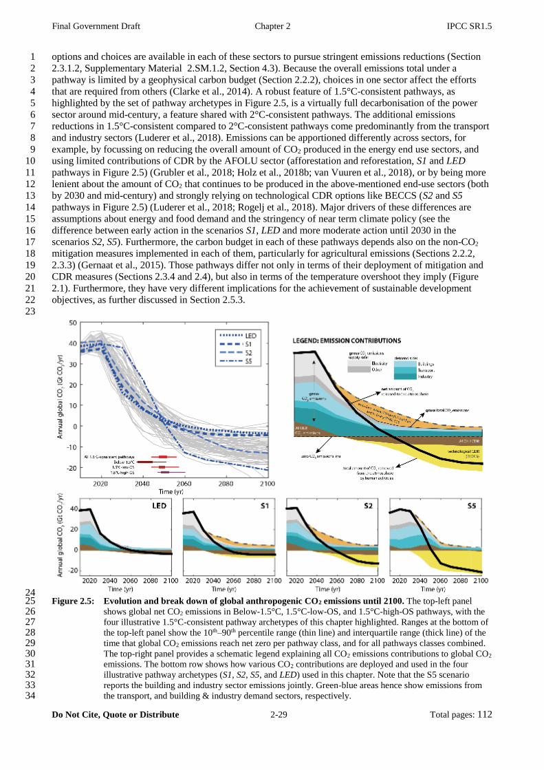
Final Government Draft Chapter 2 IPCC SR1.5
Do Not Cite, Quote or Distribute 2-29 Total pages: 112
options and choices are available in each of these sectors to pursue stringent emissions reductions (Section 1
2.3.1.2, Supplementary Material 2.SM.1.2, Section 4.3). Because the overall emissions total under a 2
pathway is limited by a geophysical carbon budget (Section 2.2.2), choices in one sector affect the efforts 3
that are required from others (Clarke et al., 2014). A robust feature of 1.5°C-consistent pathways, as 4
highlighted by the set of pathway archetypes in Figure 2.5, is a virtually full decarbonisation of the power 5
sector around mid-century, a feature shared with 2°C-consistent pathways. The additional emissions 6
reductions in 1.5°C-consistent compared to 2°C-consistent pathways come predominantly from the transport 7
and industry sectors (Luderer et al., 2018). Emissions can be apportioned differently across sectors, for 8
example, by focussing on reducing the overall amount of CO2 produced in the energy end use sectors, and 9
using limited contributions of CDR by the AFOLU sector (afforestation and reforestation, S1 and LED 10
pathways in Figure 2.5) (Grubler et al., 2018; Holz et al., 2018b; van Vuuren et al., 2018), or by being more 11
lenient about the amount of CO2 that continues to be produced in the above-mentioned end-use sectors (both 12
by 2030 and mid-century) and strongly relying on technological CDR options like BECCS (S2 and S5 13
pathways in Figure 2.5) (Luderer et al., 2018; Rogelj et al., 2018). Major drivers of these differences are 14
assumptions about energy and food demand and the stringency of near term climate policy (see the 15
difference between early action in the scenarios S1, LED and more moderate action until 2030 in the 16
scenarios S2, S5). Furthermore, the carbon budget in each of these pathways depends also on the non-CO2 17
mitigation measures implemented in each of them, particularly for agricultural emissions (Sections 2.2.2, 18
2.3.3) (Gernaat et al., 2015). Those pathways differ not only in terms of their deployment of mitigation and 19
CDR measures (Sections 2.3.4 and 2.4), but also in terms of the temperature overshoot they imply (Figure 20
2.1). Furthermore, they have very different implications for the achievement of sustainable development 21
objectives, as further discussed in Section 2.5.3. 22
23
24 Figure 2.5: Evolution and break down of global anthropogenic CO2 emissions until 2100. The top-left panel 25
shows global net CO2 emissions in Below-1.5°C, 1.5°C-low-OS, and 1.5°C-high-OS pathways, with the 26 four illustrative 1.5°C-consistent pathway archetypes of this chapter highlighted. Ranges at the bottom of 27 the top-left panel show the 10th–90th percentile range (thin line) and interquartile range (thick line) of the 28 time that global CO2 emissions reach net zero per pathway class, and for all pathways classes combined. 29 The top-right panel provides a schematic legend explaining all CO2 emissions contributions to global CO2 30 emissions. The bottom row shows how various CO2 contributions are deployed and used in the four 31 illustrative pathway archetypes (S1, S2, S5, and LED) used in this chapter. Note that the S5 scenario 32 reports the building and industry sector emissions jointly. Green-blue areas hence show emissions from 33 the transport, and building & industry demand sectors, respectively. 34
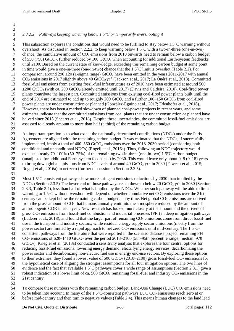
Final Government Draft Chapter 2 IPCC SR1.5
Do Not Cite, Quote or Distribute 2-30 Total pages: 112
1
2
Pathways keeping warming below 1.5°C or temporarily overshooting it 3
4
This subsection explores the conditions that would need to be fulfilled to stay below 1.5°C warming without 5
overshoot. As discussed in Section 2.2.2, to keep warming below 1.5°C with a two-in-three (one-in-two) 6
chance, the cumulative amount of CO2 emissions from 2018 onwards need to remain below a carbon budget 7
of 550 (750) GtCO2, further reduced by 100 GtCO2 when accounting for additional Earth-system feedbacks 8
until 2100. Based on the current state of knowledge, exceeding this remaining carbon budget at some point 9
in time would give a one-in-three (one-in-two) chance that the 1.5°C limit is overshot (Table 2.2). For 10
comparison, around 290 ±20 (1-sigma range) GtCO2 have been emitted in the years 2011-2017 with annual 11
CO2 emissions in 2017 slightly above 40 GtCO2 yr-1 (Jackson et al., 2017; Le Quéré et al., 2018). Committed 12
fossil-fuel emissions from existing fossil-fuel infrastructure as of 2010 have been estimated at around 500 13
±200 GtCO2 (with ca. 200 GtCO2 already emitted until 2017) (Davis and Caldeira, 2010). Coal-fired power 14
plants contribute the largest part. Committed emissions from existing coal-fired power plants built until the 15
end of 2016 are estimated to add up to roughly 200 GtCO2 and a further 100–150 GtCO2 from coal-fired 16
power plants are under construction or planned (González-Eguino et al., 2017; Edenhofer et al., 2018). 17
However, there has been a marked slowdown of planned coal-power projects in recent years, and some 18
estimates indicate that the committed emissions from coal plants that are under construction or planned have 19
halved since 2015 (Shearer et al., 2018). Despite these uncertainties, the committed fossil-fuel emissions are 20
assessed to already amount to more than half (a third) of the remaining carbon budget. 21
22
An important question is to what extent the nationally determined contributions (NDCs) under the Paris 23
Agreement are aligned with the remaining carbon budget. It was estimated that the NDCs, if successfully 24
implemented, imply a total of 400–560 GtCO2 emissions over the 2018–2030 period (considering both 25
conditional and unconditional NDCs) (Rogelj et al., 2016a). Thus, following an NDC trajectory would 26
exhaust already 70–100% (50–75%) of the remaining two-in-three (one-in-two) 1.5°C carbon budget 27
(unadjusted for additional Earth-system feedbacks) by 2030. This would leave only about 0–8 (9–18) years 28
to bring down global emissions from NDC levels of around 40 GtCO2 yr-1 in 2030 (Fawcett et al., 2015; 29
Rogelj et al., 2016a) to net zero (further discussion in Section 2.3.5). 30
31
Most 1.5°C-consistent pathways show more stringent emissions reductions by 2030 than implied by the 32
NDCs (Section 2.3.5) The lower end of those pathways reach down to below 20 GtCO2 yr-1 in 2030 (Section 33
2.3.3, Table 2.4), less than half of what is implied by the NDCs. Whether such pathway will be able to limit 34
warming to 1.5°C without overshoot will depend on whether cumulative net CO2 emissions over the 21st 35
century can be kept below the remaining carbon budget at any time. Net global CO2 emissions are derived 36
from the gross amount of CO2 that humans annually emit into the atmosphere reduced by the amount of 37
anthropogenic CDR in each year. New research has looked more closely at the amount and the drivers of 38
gross CO2 emissions from fossil-fuel combustion and industrial processes (FFI) in deep mitigation pathways 39
(Luderer et al., 2018), and found that the larger part of remaining CO2 emissions come from direct fossil-fuel 40
use in the transport and industry sectors, while residual energy supply sector emissions (mostly from the 41
power sector) are limited by a rapid approach to net zero CO2 emissions until mid-century. The 1.5°C-42
consistent pathways from the literature that were reported in the scenario database project remaining FFI 43
CO2 emissions of 620–1410 GtCO2 over the period 2018–2100 (5th–95th percentile range; median: 970 44
GtCO2). Kriegler et al. (2018a) conducted a sensitivity analysis that explores the four central options for 45
reducing fossil-fuel emissions: lowering energy demand, electrifying energy services, decarbonizing the 46
power sector and decarbonizing non-electric fuel use in energy end-use sectors. By exploring these options 47
to their extremes, they found a lowest value of 500 GtCO2 (2018–2100) gross fossil-fuel CO2 emissions for 48
the hypothetical case of aligning the strongest assumptions for all four mitigation options. The two lines of 49
evidence and the fact that available 1.5°C pathways cover a wide range of assumptions (Section 2.3.1) give a 50
robust indication of a lower limit of ca. 500 GtCO2 remaining fossil-fuel and industry CO2 emissions in the 51
21st century. 52
53
To compare these numbers with the remaining carbon budget, Land-Use Change (LUC) CO2 emissions need 54
to be taken into account. In many of the 1.5°C-consistent pathways LUC CO2 emissions reach zero at or 55
before mid-century and then turn to negative values (Table 2.4). This means human changes to the land lead 56

Final Government Draft Chapter 2 IPCC SR1.5
Do Not Cite, Quote or Distribute 2-31 Total pages: 112
to atmospheric carbon being stored in plants and soils. This needs to be distinguished from the natural CO2 1
uptake by land which is not accounted for in the anthropogenic LUC CO2 emissions reported in the 2
pathways. Given the difference in estimating the ‘anthropogenic’ sink between countries and the global 3
integrated assessment and carbon modelling community (Grassi et al., 2017), the LUC CO2 estimates 4
included here are not necessarily directly comparable with countries' estimates at global level. The 5
cumulated amount of LUC CO2 emissions until the time they reach zero combine with the fossil-fuel and 6
industry CO2 emissions to a total amount of gross emissions of 670–1430 GtCO2 for the period 2018–2100 7
(5th–95th percentile; median 1040 GtCO2). The lower end of the range is similar to what emerges from a 8
scenario of transformative change that halves CO2 emissions every decade from 2020 to 2050 (Rockström et 9
al., 2017). All these estimates are above the remaining carbon budget for a two-in-three chance of limiting 10
warming below 1.5°C without overshoot, including the low end of the hypothetical sensitivity analysis of 11
Kriegler et al. (2018a), who assumes 75 GtCO2 LUC emissions adding to a total of 575 GtCO2 gross CO2 12
emissions. As only limited, highly idealized cases have been identified that keep gross CO2 emissions within 13
the 1.5°C carbon budget and based on current understanding of the geophysical response and its 14
uncertainties, the available evidence indicates that avoiding overshoot will require some type of CDR in a 15
broad sense, e.g., via negative LUC CO2 emissions. (medium confidence) (Table 2.2). 16
17
Net CO2 emissions can fall below gross CO2 emissions, if CDR is brought into the mix. Studies have looked 18
at mitigation and CDR in combination to identify strategies for limiting warming to 1.5°C (Sanderson et al., 19
2016; Ricke et al., 2017). CDR and/or negative LUC CO2 emissions are deployed by all 1.5°C-consistent 20
pathways available to this assessment, but the scale of deployment and choice of CDR measure varies widely 21
(Section 2.3.4). Furthermore, no CDR technology has been deployed at scale yet, and all come with concerns 22
about their potential (Fuss et al., 2018), feasibility (Nemet et al., 2018) and/or sustainability (Smith et al., 23
2015; Fuss et al., 2018) (see Sections 2.3.4, 4.3.2 and 4.3.7 and Cross-Chapter Box 7 in Chapter3 for further 24
discussion). CDR can have two very different functions in 1.5°C-consistent pathways. If deployed in the first 25
half of the century, before net zero CO2 emissions are reached, it neutralizes some of the remaining CO2 26
emissions year by year and thus slows the accumulation of CO2 in the atmosphere. In this first function it can 27
be used to remain within the carbon budget and avoid overshoot. If CDR is deployed in the second half of 28
the century after carbon neutrality has been established, it can still be used to neutralize some residual 29
emissions from other sectors, but also to create net negative emissions that actively draw down the 30
cumulative amount of CO2 emissions to return below a 1.5°C warming level. In the second function, CDR 31
enables temporary overshoot. The literature points to strong limitations to upscaling CDR (limiting its first 32
abovementioned function) and to sustainability constraints (limiting both abovementioned functions) (Fuss et 33
al., 2018; Minx et al., 2018; Nemet et al., 2018). Large uncertainty hence exists about what amount of CDR 34
could actually be available before mid-century. Kriegler et al. (2018a) explore a case limiting CDR to 100 35
GtCO2 until 2050, and the 1.5°C-consistent pathways available in the report’s database project 40–260 36
GtCO2 CDR until the point of carbon neutrality (5th to 95th percentile; median 120 GtCO2). Because gross 37
CO2 emissions in most cases exceed the remaining carbon budget by several hundred GtCO2 and given the 38
limits to CDR deployment until 2050, most of the 1.5°C-consistent pathways available to this assessment are 39
overshoot pathways. However, the scenario database also contains nine non-overshoot pathways that remain 40
below 1.5°C throughout the 21st century and that are assessed in the chapter. 41
42
43
2.3.3 Emissions evolution in 1.5°C pathways 44
45
This section assesses the salient temporal evolutions of climate forcers over the 21st century. It uses the 46
classification of 1.5°C-consisten pathways presented in Section 2.1, which includes a Below-1.5°C class, as 47
well as other classes with varying levels of projected overshoot (1.5°C-low-OS and 1.5°C-high-OS). First, 48
aggregate-GHG benchmarks for 2030 are assessed. Subsequent sections assess long-lived climate forcers 49
(LLCF) and short-lived climate forcers (SLCF) separately because they contribute in different ways to near-50
term, peak and long-term warming (Section 2.2, Cross-Chapter Box 2 in Chapter 1). 51
52
Estimates of aggregated GHG emissions in line with specific policy choices are often compared to near-term 53
benchmark values from mitigation pathways to explore their consistency with long-term climate goals 54
(Clarke et al., 2014; UNEP, 2016, 2017; UNFCCC, 2016). Benchmark emissions or estimates of peak years 55
derived from IAMs provide guidelines or milestones that are consistent with achieving a given temperature 56
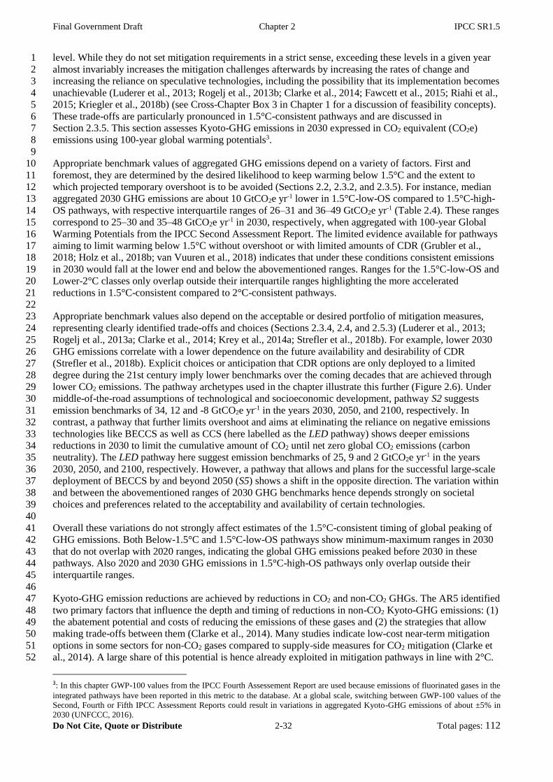
Final Government Draft Chapter 2 IPCC SR1.5
Do Not Cite, Quote or Distribute 2-32 Total pages: 112
level. While they do not set mitigation requirements in a strict sense, exceeding these levels in a given year 1
almost invariably increases the mitigation challenges afterwards by increasing the rates of change and 2
increasing the reliance on speculative technologies, including the possibility that its implementation becomes 3
unachievable (Luderer et al., 2013; Rogelj et al., 2013b; Clarke et al., 2014; Fawcett et al., 2015; Riahi et al., 4
2015; Kriegler et al., 2018b) (see Cross-Chapter Box 3 in Chapter 1 for a discussion of feasibility concepts). 5
These trade-offs are particularly pronounced in 1.5°C-consistent pathways and are discussed in 6
Section 2.3.5. This section assesses Kyoto-GHG emissions in 2030 expressed in CO2 equivalent (CO2e) 7
emissions using 100-year global warming potentials3. 8
9
Appropriate benchmark values of aggregated GHG emissions depend on a variety of factors. First and 10
foremost, they are determined by the desired likelihood to keep warming below 1.5°C and the extent to 11
which projected temporary overshoot is to be avoided (Sections 2.2, 2.3.2, and 2.3.5). For instance, median 12
aggregated 2030 GHG emissions are about 10 GtCO2e yr-1 lower in 1.5°C-low-OS compared to 1.5°C-high-13
OS pathways, with respective interquartile ranges of 26–31 and 36–49 GtCO2e yr-1 (Table 2.4). These ranges 14
correspond to 25–30 and 35–48 GtCO2e yr-1 in 2030, respectively, when aggregated with 100-year Global 15
Warming Potentials from the IPCC Second Assessment Report. The limited evidence available for pathways 16
aiming to limit warming below 1.5°C without overshoot or with limited amounts of CDR (Grubler et al., 17
2018; Holz et al., 2018b; van Vuuren et al., 2018) indicates that under these conditions consistent emissions 18
in 2030 would fall at the lower end and below the abovementioned ranges. Ranges for the 1.5°C-low-OS and 19
Lower-2°C classes only overlap outside their interquartile ranges highlighting the more accelerated 20
reductions in 1.5°C-consistent compared to 2°C-consistent pathways. 21
22
Appropriate benchmark values also depend on the acceptable or desired portfolio of mitigation measures, 23
representing clearly identified trade-offs and choices (Sections 2.3.4, 2.4, and 2.5.3) (Luderer et al., 2013; 24
Rogelj et al., 2013a; Clarke et al., 2014; Krey et al., 2014a; Strefler et al., 2018b). For example, lower 2030 25
GHG emissions correlate with a lower dependence on the future availability and desirability of CDR 26
(Strefler et al., 2018b). Explicit choices or anticipation that CDR options are only deployed to a limited 27
degree during the 21st century imply lower benchmarks over the coming decades that are achieved through 28
lower CO2 emissions. The pathway archetypes used in the chapter illustrate this further (Figure 2.6). Under 29
middle-of-the-road assumptions of technological and socioeconomic development, pathway S2 suggests 30
emission benchmarks of 34, 12 and -8 GtCO2e yr-1 in the years 2030, 2050, and 2100, respectively. In 31
contrast, a pathway that further limits overshoot and aims at eliminating the reliance on negative emissions 32
technologies like BECCS as well as CCS (here labelled as the LED pathway) shows deeper emissions 33
reductions in 2030 to limit the cumulative amount of CO2 until net zero global CO2 emissions (carbon 34
neutrality). The LED pathway here suggest emission benchmarks of 25, 9 and 2 GtCO2e yr-1 in the years 35
2030, 2050, and 2100, respectively. However, a pathway that allows and plans for the successful large-scale 36
deployment of BECCS by and beyond 2050 (S5) shows a shift in the opposite direction. The variation within 37
and between the abovementioned ranges of 2030 GHG benchmarks hence depends strongly on societal 38
choices and preferences related to the acceptability and availability of certain technologies. 39
40
Overall these variations do not strongly affect estimates of the 1.5°C-consistent timing of global peaking of 41
GHG emissions. Both Below-1.5°C and 1.5°C-low-OS pathways show minimum-maximum ranges in 2030 42
that do not overlap with 2020 ranges, indicating the global GHG emissions peaked before 2030 in these 43
pathways. Also 2020 and 2030 GHG emissions in 1.5°C-high-OS pathways only overlap outside their 44
interquartile ranges. 45
46
Kyoto-GHG emission reductions are achieved by reductions in CO2 and non-CO2 GHGs. The AR5 identified 47
two primary factors that influence the depth and timing of reductions in non-CO2 Kyoto-GHG emissions: (1) 48
the abatement potential and costs of reducing the emissions of these gases and (2) the strategies that allow 49
making trade-offs between them (Clarke et al., 2014). Many studies indicate low-cost near-term mitigation 50
options in some sectors for non-CO2 gases compared to supply-side measures for CO2 mitigation (Clarke et 51
al., 2014). A large share of this potential is hence already exploited in mitigation pathways in line with 2°C. 52
3: In this chapter GWP-100 values from the IPCC Fourth Assessement Report are used because emissions of fluorinated gases in the
integrated pathways have been reported in this metric to the database. At a global scale, switching between GWP-100 values of the
Second, Fourth or Fifth IPCC Assessment Reports could result in variations in aggregated Kyoto-GHG emissions of about ±5% in
2030 (UNFCCC, 2016).
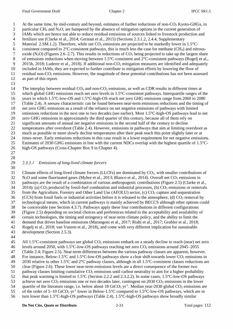
Final Government Draft Chapter 2 IPCC SR1.5
Do Not Cite, Quote or Distribute 2-33 Total pages: 112
At the same time, by mid-century and beyond, estimates of further reductions of non-CO2 Kyoto-GHGs, in 1
particular CH4 and N2O, are hampered by the absence of mitigation options in the current generation of 2
IAMs which are hence not able to reduce residual emissions of sources linked to livestock production and 3
fertilizer use (Clarke et al., 2014; Gernaat et al., 2015) (Sections 2.3.1.2, 2.4.4, Supplementary 4
Material 2.SM.1.2). Therefore, while net CO2 emissions are projected to be markedly lower in 1.5°C-5
consistent compared to 2°C-consistent pathways, this is much less the case for methane (CH4) and nitrous-6
oxide (N2O) (Figures 2.6–2.7). This results in reductions of CO2 being projected to take up the largest share 7
of emissions reductions when moving between 1.5°C-consistent and 2°C-consistent pathways (Rogelj et al., 8
2015b, 2018; Luderer et al., 2018). If additional non-CO2 mitigation measures are identified and adequately 9
included in IAMs, they are expected to further contribute to mitigation efforts by lowering the floor of 10
residual non-CO2 emissions. However, the magnitude of these potential contributions has not been assessed 11
as part of this report. 12
13
The interplay between residual CO2 and non-CO2 emissions, as well as CDR results in different times at 14
which global GHG emissions reach net zero levels in 1.5°C-consistent pathways. Interquartile ranges of the 15
years in which 1.5°C-low-OS and 1.5°C-high-OS reach net zero GHG emissions range from 2060 to 2080 16
(Table 2.4). A seesaw characteristic can be found between near-term emissions reductions and the timing of 17
net zero GHG emissions as a result of the reliance on net negative emissions of pathways with limited 18
emissions reductions in the next one to two decades (see earlier). Most 1.5°C-high-OS pathways lead to net 19
zero GHG emissions in approximately the third quarter of this century, because all of them rely on 20
significant amounts of annual net negative emissions in the second half of the century to decline 21
temperatures after overshoot (Table 2.4). However, emissions in pathways that aim at limiting overshoot as 22
much as possible or more slowly decline temperatures after their peak reach this point slightly later or at 23
times never. Early emissions reductions in this case result in a lower requirement for net negative emissions. 24
Estimates of 2030 GHG emissions in line with the current NDCs overlap with the highest quartile of 1.5°C-25
high-OS pathways (Cross-Chapter Box 9 in Chapter 4). 26
27
28
Emissions of long-lived climate forcers 29
30
Climate effects of long-lived climate forcers (LLCFs) are dominated by CO2, with smaller contributions of 31
N2O and some fluorinated gases (Myhre et al., 2013; Blanco et al., 2014). Overall net CO2 emissions in 32
pathways are the result of a combination of various anthropogenic contributions (Figure 2.5) (Clarke et al., 33
2014): (a) CO2 produced by fossil-fuel combustion and industrial processes, (b) CO2 emissions or removals 34
from the Agriculture, Forestry and Other Land Use (AFOLU) sector, (c) CO2 capture and sequestration 35
(CCS) from fossil fuels or industrial activities before it is released to the atmosphere, (d) CO2 removal by 36
technological means, which in current pathways is mainly achieved by BECCS although other options could 37
be conceivable (see Section 4.3.7). Pathways apply these four contributions in different configurations 38
(Figure 2.5) depending on societal choices and preferences related to the acceptability and availability of 39
certain technologies, the timing and stringency of near-term climate policy, and the ability to limit the 40
demand that drives baseline emissions (Marangoni et al., 2017; Riahi et al., 2017; Grubler et al., 2018; 41
Rogelj et al., 2018; van Vuuren et al., 2018), and come with very different implication for sustainable 42
development (Section 2.5.3). 43
44
All 1.5°C-consistent pathways see global CO2 emissions embark on a steady decline to reach (near) net zero 45
levels around 2050, with 1.5°C-low-OS pathways reaching net zero CO2 emissions around 2045–2055 46
(Table 2.4; Figure 2.5). Near-term differences between the various pathway classes are apparent, however. 47
For instance, Below-1.5°C and 1.5°C-low-OS pathways show a clear shift towards lower CO2 emissions in 48
2030 relative to other 1.5°C and 2°C pathway classes, although in all 1.5°C-consistent classes reductions are 49
clear (Figure 2.6). These lower near-term emissions levels are a direct consequence of the former two 50
pathway classes limiting cumulative CO2 emissions until carbon neutrality to aim for a higher probability 51
that peak warming is limited to 1.5°C (Section 2.2.2 and 2.3.2.2). In some cases, 1.5°C-low-OS pathways 52
achieve net zero CO2 emissions one or two decades later, contingent on 2030 CO2 emissions in the lower 53
quartile of the literature range, i.e. below about 18 GtCO2 yr-1. Median year-2030 global CO2 emissions are 54
of the order of 5–10 GtCO2 yr-1 lower in Below-1.5°C compared to 1.5°C-low-OS pathways, which are in 55
turn lower than 1.5°C-high-OS pathways (Table 2.4). 1.5°C-high-OS pathways show broadly similar 56

Final Government Draft Chapter 2 IPCC SR1.5
Do Not Cite, Quote or Distribute 2-34 Total pages: 112
emissions levels than the 2°C-consistent pathways in 2030. 1
2
The development of CO2 emissions in the second half of the century in 1.5°C pathways is characterised by 3
the need to stay or return within a carbon budget. Figure 2.6 shows net CO2 and N2O emissions from various 4
sources in 2050 and 2100 in 1.5°C-consistent pathways in the literature. Virtually all 1.5°C pathways obtain 5
net negative CO2 emissions at some point during the 21st century but the extent to which net negative 6
emissions are relied upon varies substantially (Figure 2.6, Table 2.4). This net withdrawal of CO2 from the 7
atmosphere compensates for residual long-lived non-CO2 GHG emissions that also accumulate in the 8
atmosphere (like N2O) or to cancel some of the build-up of CO2 due to earlier emissions to achieve 9
increasingly higher likelihoods that warming stays or returns below 1.5°C (see Section 2.3.4 for a discussion 10
of various uses of CDR). Even non-overshoot pathways that aim at achieving temperature stabilisation 11
would hence deploy a certain amount of net negative emissions to offset any accumulating long-lived non-12
CO2 GHGs. 1.5°C overshoot pathways display significantly larger amounts of annual net negative emissions 13
in the second half of the century. The larger the overshoot the more net negative emissions are required to 14
return temperatures to 1.5°C by the end of the century (Table 2.4, Figure 2.1). 15
16
N2O emissions decline to a much lesser extent than CO2 in currently available 1.5°C-consistent pathways 17
(Figure 2.6). Current IAMs have limited emissions reduction potentials (Gernaat et al., 2015) (Sections 18
2.3.1.2, 2.4.4, Supplementary Material 2.SM.1.2), reflecting the difficulty of eliminating N2O emission from 19
agriculture (Bodirsky et al., 2014). Moreover, the reliance of some pathways on significant amounts of 20
bioenergy after mid-century (Section 2.4.2) coupled to a substantial use of nitrogen fertilizer (Popp et al., 21
2017) also makes reducing N2O emissions harder (for example, see pathway S5 in Figure 2.6). As a result, 22
sizeable residual N2O emissions are currently projected to continue throughout the century, and measures to 23
effectively mitigate them will be of continued relevance for 1.5°C societies. Finally, the reduction of 24
nitrogen use and N2O emissions from agriculture is already a present-day concern due to unsustainable levels 25
of nitrogen pollution (Bodirsky et al., 2012). Section 2.4.4 provides a further assessment of the agricultural 26
non-CO2 emissions reduction potential. 27

Final Government Draft Chapter 2 IPCC SR1.5
Do Not Cite, Quote or Distribute 2-35 Total pages: 112
Figure 2.6: Annual global emissions characteristics for 2020, 2030, 2050, 2100. Data are shown for Kyoto-GHG 1
emissions (top panel), and total CO2 emissions, CO2 emissions from the AFOLU sector, global N2O 2 emissions, and CO2 emissions from fossil-fuel use and industrial processes. The latter is also split into 3 emissions from the energy supply sector (electricity sector and refineries), and direct emissions from 4 fossil-fuel use in energy demand sectors (industry, buildings, transport) (bottom row). Horizontal black 5 lines show the median, boxes show the interquartile range, and whiskers the minimum-maximum range. 6 Icons indicate the four pathway archetypes used in this chapter. In case less than 7 data points are 7 available in a class, the minimum-maximum range and single data points are shown. Kyoto-GHG, 8 emissions in the top panel are aggregated with AR4 GWP-100 and contain CO2, CH4, N2O, HFCs, PFCs, 9 and SF6. NF3 is typically not reported by IAMs. Scenarios with year-2010 Kyoto-GHG emissions outside 10

Final Government Draft Chapter 2 IPCC SR1.5
Do Not Cite, Quote or Distribute 2-36 Total pages: 112
the range assessed by IPCC AR5 WGIII assessed are excluded (IPCC, 2014b).. 1 2 3
Emissions of short-lived climate forcers and fluorinated gases 4
5
SLCFs include shorter-lived GHGs like CH4 and some HFCs, as well as particles (aerosols), their precursors 6
and ozone precursors. SLCFs are strongly mitigated in 1.5°C pathways as is the case for 2°C pathways 7
(Figure 2.7). SLCF emissions ranges of 1.5°C and 2°C pathway classes strongly overlap, indicating that the 8
main incremental mitigation contribution between 1.5°C and 2°C pathways comes from CO2 (Luderer et al., 9
2018; Rogelj et al., 2018). CO2 and SLCF emissions reductions are connected in situations where SLCF and 10
CO2 are co-emitted by the same process, for example, with coal-fired power plants (Shindell and Faluvegi, 11
2010) or within the transport sector (Fuglestvedt et al., 2010). Many CO2-targeted mitigation measures in 12
industry, transport and agriculture (Sections 2.4.3–4) hence also reduce non-CO2 forcing (Rogelj et al., 13
2014b; Shindell et al., 2016). 14
15
Despite having a strong warming effect (Myhre et al., 2013; Etminan et al., 2016), current 1.5°C-consistent 16
pathways still project significant emissions of CH4 by 2050, indicating that only limited mitigation options 17
are included and identified in IAM analyses (Gernaat et al., 2015) (Sections 2.3.1.2, 2.4.4, Table 2.SM.2). 18
The AFOLU sector contributes an important share of the residual CH4 emissions until mid-century, with its 19
relative share increasing from slightly below 50% in 2010 to roughly around 55–70% in 2030, and 60–80% 20
in 2050 in 1.5°C-consistent pathways (interquartile range across 1.5°C-consistent pathways for projections). 21
Many of the proposed measures to target CH4 (Shindell et al., 2012; Stohl et al., 2015) are included in 1.5°C-22
consistent pathways (Figure 2.7), though not all (Sections 2.3.1.2, 2.4.4, Table 2.SM.2). A detailed 23
assessment of measures to further reduce AFOLU CH4 emissions has not been conducted. 24
25
Overall reductions of SLCFs can have effects of either sign on temperature depending on the balance 26
between cooling and warming agents. The reduction in SO2 emissions is the dominant single effect as it 27
weakens the negative total aerosol forcing. This means that reducing all SLCF emissions to zero would result 28
in a short-term warming, although this warming is unlikely to be more than 0.5°C (Section 2.2 and Figure 29
1.5 (Samset et al., 2018)). Because of this effect, suggestions have been proposed that target the warming 30
agents only (referred to as short-lived climate pollutants or SLCPs instead of the more general short-lived 31
climate forcers; e.g., Shindell et al., 2012) though aerosols are often emitted in varying mixtures of warming 32
and cooling species (Bond et al., 2013). Black Carbon (BC) emissions reach similar levels across 1.5°C-33
consistent and 2°C-consistent pathways available in the literature, with interquartile ranges of emissions 34
reductions across pathways of 16–34% and 48–58% in 2030 and 2050, respectively, relative to 2010 (Figure 35
2.7). Recent studies have identified further reduction potentials for the near term, with global reductions of 36
about 80% being suggested (Stohl et al., 2015; Klimont et al., 2017). Because the dominant sources of 37
certain aerosol mixtures are emitted during the combustion of fossil fuels, the rapid phase-out of unabated 38
fossil-fuels to avoid CO2 emissions would also result in removal of these either warming or cooling SLCF 39
air-pollutant species. Furthermore, they are also reduced by efforts to reduce particulate air pollution. For 40
example, year-2050 SO2 emissions, precursor of sulphate aerosol, in 1.5°C-consistent pathways are about 41
75–85% lower than their 2010 levels. Some caveats apply, for example, if residential biomass use would be 42
encouraged in industrialised countries in stringent mitigation pathways without appropriate pollution control 43
measures, aerosol concentrations could also increase (Sand et al., 2015; Stohl et al., 2015). 44

Final Government Draft Chapter 2 IPCC SR1.5
Do Not Cite, Quote or Distribute 2-37 Total pages: 112
Table 2.4: Emissions in 2030, 2050 and 2100 in 1.5°C and 2°C scenario classes and absolute annual rates of change between 2010–2030, 2020–2030 and 2030–2050, 1 respectively. Values show: median (25th and 75th percentile), across available scenarios. If less than seven scenarios are available (*), the minimum-maximum range is 2 given instead. For the timing of global zero of total net CO2 and Kyoto-GHG emissions, the interquartile range is given. Kyoto-GHG emissions are aggregated with 3 GWP-100 values from IPCC AR4. 2010 emissions for total net CO2, CO2 from fossil-fuel use & industry, and AFOLU CO2 are estimated at 38.5, 33.4, and 5 GtCO2/yr, 4 respectively (Le Quéré et al., 2018). A difference is reported in estimating the "anthropogenic" sink by countries or the global carbon modelling community (Grassi et 5 al., 2017), and AFOLU CO2 estimates reported here are thus not necessarily comparable with countries' estimates. Scenarios with year-2010 Kyoto-GHG emissions 6 outside the range assessed by IPCC AR5 WGIII are excluded (IPCC, 2014b). 7
type Absolute annual change (GtCO2/yr) Timing of global zero
name category count 2030 2050 2100 2010-2030 2020-2030 2030-2050 year
Total CO2 (net) Below-1.5°C 5 13 (11 15) -3 (-11 2) -8 (-14 -3) -1.2 (-1.3 -1.0) -2.5 (-2.8 -1.8) -0.8 (-1.2 -0.7) (2037 2054)
1.5°C-low-OS 37 21 (18 22) 0 (-2 3) -11 (-14 -8) -0.8 (-1 -0.7) -1.7 (-2.3 -1.4) -1 (-1.2 -0.8) (2047 2055)
1.5°C-high-OS 36 29 (26 36) 1 (-1 6) -14 (-16 -11) -0.4 (-0.6 0) -1.1 (-1.5 -0.5) -1.3 (-1.8 -1.1) (2049 2059)
Lower-2°C 67 27 (22 30) 9 (7 13) -4 (-9 0) -0.5 (-0.7 -0.3) -1.2 (-1.9 -0.9) -0.8 (-1 -0.6) (2065 2096)
Higher-2°C 54 33 (31 35) 18 (12 19) -3 (-11 1) -0.2 (-0.4 0) -0.7 (-0.9 -0.5) -0.8 (-1 -0.6) (2070 post-2100)
CO2 from fossil
fuels and industry
(gross)
Below-1.5°C 5 18 (14 21) 10 (0 21) 8 (0 12) -0.7 (-1.0 -0.6) -1.5 (-2.2 -0.9) -0.4 (-0.7 -0.0) -
1.5°C-low-OS 37 22 (19 24) 10 (8 14) 6 (3 8) -0.5 (-0.6 -0.4) -1.3 (-1.7 -0.9) -0.6 (-0.7 -0.5) -
1.5°C-high-OS 36 28 (26 37) 13 (12 17) 7 (3 9) -0.2 (-0.3 0.2) -0.8 (-1.1 -0.2) -0.7 (-1 -0.6) -
Lower-2°C 67 26 (21 31) 14 (11 18) 8 (4 10) -0.3 (-0.6 -0.1) -0.9 (-1.4 -0.6) -0.6 (-0.7 -0.4) -
Higher-2°C 54 31 (29 33) 19 (17 23) 8 (5 11) -0.1 (-0.2 0.1) -0.5 (-0.7 -0.2) -0.6 (-0.7 -0.5) -
CO2 from fossil
fuels and industry
(net)
Below-1.5°C 5 16 (13 18) 1 (0 7) -3 (-10 0) -0.8 (-1.0 -0.7) -1.8 (-2.2 -1.2) -0.6 (-0.9 -0.5) -
1.5°C-low-OS 37 21 (18 22) 3 (-1 6) -9 (-12 -4) -0.6 (-0.7 -0.5) -1.4 (-1.8 -1.1) -0.8 (-1.1 -0.7) -
1.5°C-high-OS 36 27 (25 35) 4 (1 10) -11 (-13 -7) -0.3 (-0.3 0.1) -0.9 (-1.2 -0.3) -1.2 (-1.5 -0.9) -
Lower-2°C 67 26 (21 30) 11 (8 14) -2 (-5 2) -0.3 (-0.6 -0.1) -1 (-1.4 -0.6) -0.7 (-1 -0.4) -
Higher-2°C 54 31 (29 33) 17 (13 19) -3 (-8 3) -0.1 (-0.2 0.1) -0.5 (-0.7 -0.2) -0.7 (-1 -0.5) -
CO2 from AFOLU Below-1.5°C 5 -2 (-5 0) -4 (-11 -1) -4 (-5 -3) -0.3 (-0.4 -0.2) -0.5 (-0.8 -0.4) -0.1 (-0.4 0) -
1.5°C-low-OS 37 0 (-1 1) -2 (-4 -1) -2 (-4 -1) -0.2 (-0.3 -0.2) -0.4 (-0.5 -0.3) -0.1 (-0.2 -0.1) -
1.5°C-high-OS 36 1 (0 3) -2 (-5 0) -2 (-5 -1) -0.1 (-0.3 -0.1) -0.2 (-0.5 -0.1) -0.2 (-0.3 0) -
Lower-2°C 67 1 (0 2) -2 (-3 -1) -2 (-4 -1) -0.2 (-0.3 -0.1) -0.3 (-0.4 -0.2) -0.2 (-0.2 -0.1) -
Higher-2°C 54 2 (1 3) 0 (-2 2) -1 (-4 0) -0.2 (-0.2 -0.1) -0.2 (-0.4 -0.1) -0.1 (-0.1 0) -
Bioenergy
combined with
carbon capture and
storage (BECCS)
Below-1.5°C 5 0 (-1 0) -3 (-8 0) -6 (-13 0) 0 (-0.1 0) 0 (-0.1 0) -0.2 (-0.4 0) -
1.5°C-low-OS 37 0 (-1 0) -5 (-6 -4) -12 (-16 -7) 0 (-0.1 0) 0 (-0.1 0) -0.2 (-0.3 -0.2) -
1.5°C-high-OS 36 0 (0 0) -7 (-9 -4) -15 (-16 -12) 0 (0 0) 0 (0 0) -0.3 (-0.4 -0.2) -
Lower-2°C 54 0 (0 0) -4 (-5 -2) -10 (-12 -7) 0 (0 0) 0 (0 0) -0.2 (-0.2 -0.1) -
Higher-2°C 47 0 (0 0) -3 (-5 -2) -11 (-15 -8) 0 (0 0) 0 (0 0) -0.1 (-0.2 -0.1) -
Kyoto GHG (AR4)
[GtCO2e]
Below-1.5°C 5 22 (21 23) 3 (-3 8) -3 (-11 3) -1.4 (-1.5 -1.3) -2.9 (-3.3 -2.1) -0.9 (-1.3 -0.7) (2044 post-2100)
1.5°C-low-OS 31 28 (26 31) 7 (5 10) -4 (-8 -2) -1.1 (-1.2 -0.9) -2.3 (-2.8 -1.8) -1.1 (-1.2 -0.9) (2061 2080)
1.5°C-high-OS 32 40 (36 49) 8 (6 12) -9 (-11 -6) -0.5 (-0.7 0) -1.3 (-1.8 -0.6) -1.5 (-2.1 -1.3) (2058 2067)
Lower-2°C 59 38 (31 43) 17 (14 20) 3 (0 7) -0.6 (-1 -0.3) -1.8 (-2.4 -1.1) -1 (-1.1 -0.6) (2099 post-2100)
Higher-2°C 42 45 (39 49) 26 (23 28) 5 (-5 11) -0.2 (-0.6 0) -1 (-1.2 -0.6) -1 (-1.2 -0.7) (2085 post-2100)
8

Final Government Draft Chapter 2 IPCC SR1.5
Do Not Cite, Quote or Distribute 2-38 Total pages: 112
Emissions of fluorinated gases (IPCC/TEAP, 2005; US EPA, 2013; Velders et al., 2015; Purohit and 1
Höglund-Isaksson, 2017) in 1.5°C-consistent pathways are reduced by roughly 75–80% relative to 2010 2
levels (interquartile range across 1.5°C-consistent pathways) in 2050, with no clear differences between the 3
classes. Although unabated HFC evolutions have been projected to increase (Velders et al., 2015), the Kigali 4
Amendment recently added HFCs to the basket of gases controlled under the Montreal Protocol (Höglund-5
Isaksson et al., 2017). As part of the larger group of fluorinated gases, HFCs are also assumed to decline in 6
1.5°C-consistent pathways. Projected reductions by 2050 of fluorinated gases under 1.5°C-consistent 7
pathways are deeper than published estimates of what a full implementation of the Montreal Protocol’s 8
Kigali Amendment would achieve (Höglund-Isaksson et al., 2017), which project roughly a halving of 9
fluorinated gas emissions in 2050 compared to 2010. Assuming the application of technologies that are 10
currently commercially available and at least to a limited extent already tested and implemented, potential 11
fluorinated gas emissions reductions of more than 90% have been estimated (Höglund-Isaksson et al., 2017). 12
13
There is a general agreement across 1.5°C-consistent pathways that until 2030 forcing from the warming 14
SLCFs is reduced less strongly than the net cooling forcing from aerosol effects, compared to 2010. As a 15
result, the net forcing contributions from all SLCFs combined are projected to increase slightly by about 0.2–16
0.4 W/m2, compared to 2010. Also, by the end of the century, about 0.1–0.3 W/m2 of SLCF forcing is 17
generally currently projected to remain in 1.5°C-consistent scenarios (Figure 2.8). This is similar to 18
developments in 2°C-consistent pathways (Rose et al., 2014b; Riahi et al., 2017) which show median forcing 19
contributions from these forcing agents that are generally no more than 0.1 W/m2 higher. Nevertheless, there 20
can be additional gains from targeted deeper reductions of CH4 emissions and tropospheric ozone precursors, 21
with some scenarios projecting less than 0.1 W/m2 forcing from SLCFs by 2100. 22
23
24
Figure 2.7: Global characteristics of a selection of short-lived non-CO2 emissions until mid-century for five 25 pathway classes used in this chapter. Data are shown for methane (CH4), fluorinated gases (F-gas), 26 black carbon (BC), and sulphur dioxide (SO2) emissions. Boxes with different colours refer to different 27 scenario classes. Icons on top the ranges show four illustrative pathway archetypes that apply different 28 mitigation strategies for limiting warming to 1.5°C. Boxes show the interquartile range, horizontal black 29 lines the median, while whiskers the minimum-maximum range. F-gases are expressed in units of CO2-30 equivalence computed with 100-year Global Warming Potentials reported in IPCC AR4. 31
32 33

Final Government Draft Chapter 2 IPCC SR1.5
Do Not Cite, Quote or Distribute 2-39 Total pages: 112
1 Figure 2.8: Estimated aggregated effective radiative forcing of SLCFs for 1.5°C and 2°C pathway classes in 2
2010, 2030, 2050, and 2100, as estimated by the FAIR model (Smith et al., 2018). Aggregated SLCF 3 radiative forcing is estimated as the difference between total anthropogenic radiative forcing the sum of 4 CO2 and N2O radiative forcing over time and expressed relative to 1750. Symbols indicate the four 5 pathways archetype used in this chapter. Horizontal black lines indicate the median, boxes the 6 interquartile range, and whiskers the minimum-maximum range per pathway class. Due to very few 7 pathways falling into the Below-1.5°C class, only the minimum-maximum is provided here. 8
9
10
2.3.4 CDR in 1.5°C-consistent pathways 11
12
Deep mitigation pathways assessed in AR5 showed significant deployment of CDR, in particular through 13
BECCS (Clarke et al., 2014). This has led to increased debate about the necessity, feasibility and desirability 14
of large-scale CDR deployment, sometimes also called ‘negative emissions technologies’ in the literature 15
(Fuss et al., 2014; Anderson and Peters, 2016; Williamson, 2016; van Vuuren et al., 2017a; Obersteiner et 16
al., 2018). Most CDR technologies remain largely unproven to date and raise substantial concerns about 17
adverse side-effects on environmental and social sustainability (Smith et al., 2015; Dooley and Kartha, 18
2018). A set of key questions emerge: how strongly do 1.5°C-consistent pathways rely on CDR deployment 19
and what types of CDR measures are deployed at which scale? How does this vary across available 1.5°C-20
consistent pathways and on which factors does it depend? How does CDR deployment compare between 21
1.5°C and 2°C-consistent pathways and how does it compare with the findings at the time of the AR5? How 22
does CDR deployment in 1.5°C-consistent pathways relate to questions about availability, policy 23
implementation, and sustainable development implications that have been raised about CDR technologies? 24
The first three questions are assessed in this section with the goal to provide an overview and assessment of 25
CDR deployment in the 1.5°C-consistent pathway literature. The fourth question is only touched upon here 26
and is addressed in greater depth in Section 4.3.7, which assesses the rapidly growing literature on costs, 27
potentials, availability, and sustainability implications of individual CDR measures (Minx et al., 2017, 2018; 28
Fuss et al., 2018; Nemet et al., 2018). In addition, Section 2.3.5 assesses the relationship between delayed 29
mitigation action and increased CDR reliance. CDR deployment is intricately linked to the land-use 30
transformation in 1.5°C-consistent pathways. This transformation is assessed in Section 2.4.4. Bioenergy and 31
BECCS impacts on sustainable land management are further assessed in Section 3.6.2 and Cross-Chapter 32
Box 7 in Chapter 3. Ultimately, a comprehensive assessment of the land implication of land-based CDR 33
measures will be provided in the IPCC AR6 Special Report on Climate Change and Land (SRCCL). 34
35
36
CDR technologies and deployment levels in 1.5°C-consistent pathways 37
38
A number of approaches to actively remove carbon-dioxide from the atmosphere are increasingly discussed 39
in the literature (Minx et al., 2018) (see also Section 4.3.7). Approaches under consideration include the 40

Final Government Draft Chapter 2 IPCC SR1.5
Do Not Cite, Quote or Distribute 2-40 Total pages: 112
enhancement of terrestrial and coastal carbon storage in plants and soils such as afforestation and 1
reforestation (Canadell and Raupach, 2008), soil carbon enhancement (Paustian et al., 2016; Frank et al., 2
2017; Zomer et al., 2017), and other conservation, restoration, and management options for natural and 3
managed land (Griscom et al., 2017) and coastal ecosystems (McLeod et al., 2011). Biochar sequestration 4
(Woolf et al., 2010; Smith, 2016; Werner et al., 2018) provides an additional route for terrestrial carbon 5
storage. Other approaches are concerned with storing atmospheric carbon dioxide in geological formations. 6
They include the combination of biomass use for energy production with carbon capture and storage 7
(BECCS) (Obersteiner et al., 2001; Keith and Rhodes, 2002; Gough and Upham, 2011) and direct air capture 8
with storage (DACCS) using chemical solvents and sorbents (Zeman and Lackner, 2004; Keith et al., 2006; 9
Socolow et al., 2011). Further approaches investigate the mineralisation of atmospheric carbon dioxide 10
(Mazzotti et al., 2005; Matter et al., 2016) including enhanced weathering of rocks (Schuiling and 11
Krijgsman, 2006; Hartmann et al., 2013; Strefler et al., 2018a). A fourth group of approaches is concerned 12
with the sequestration of carbon dioxide in the oceans, for example by means of ocean alkalinisation 13
(Kheshgi, 1995; Rau, 2011; Ilyina et al., 2013; Lenton et al., 2018). The costs, CDR potential and 14
environmental side effects of several of these measures are increasingly investigated and compared in the 15
literature, but large uncertainties remain, in particular concerning the feasibility and impact of large-scale 16
deployment of CDR measures (The Royal Society, 2009; Smith et al., 2015; Psarras et al., 2017; Fuss et al., 17
2018) (see Chapter 4.3.7). There are also proposals to remove methane, nitrous oxide and halocarbons via 18
photocatalysis from the atmosphere (Boucher and Folberth, 2010; de Richter et al., 2017), but a broader 19
assessment of their effectiveness, cost, and sustainability impacts is lacking to date. 20
21
Only some of these approaches have so far been considered in IAMs (see Section 2.3.1.2). The mitigation 22
scenario literature up to AR5 mostly included BECCS and to a more limited extent afforestation and 23
reforestation (Clarke et al., 2014). Since then, some 2°C and 1.5°C-consistent pathways including additional 24
CDR measures such as DACCS (Chen and Tavoni, 2013; Marcucci et al., 2017; Lehtilä and Koljonen, 2018; 25
Strefler et al., 2018b) and soil carbon sequestration (Frank et al., 2017) have become available. Other, more 26
speculative approaches, in particular ocean-based CDR and removal of non-CO2 gases, have not yet been 27
taken up by the literature on mitigation pathways. See Supplementary Material 2.SM.1.2 for an overview on 28
the coverage of CDR measures in models which contributed pathways to this assessment. Chapter 4.3.7 29
assesses the potential, costs, and sustainability implications of the full range of CDR measures. 30
31
Integrated assessment modelling has not yet explored land conservation, restoration and management options 32
to remove carbon dioxide from the atmosphere in sufficient depth, despite land management having a 33
potentially considerable impact on the terrestrial carbon stock (Erb et al., 2018). Moreover, associated CDR 34
measures have low technological requirements, and come with potential environmental and social co-35
benefits (Griscom et al., 2017). Despite the evolving capabilities of IAMs in accounting for a wider range of 36
CDR measures, 1.5°C-consistent pathways assessed here continue to predominantly rely on BECCS and 37
afforestation / reforestation (See Supplementary Material 2.SM.1.2). However, IAMs with spatially explicit 38
land-use modelling include a full accounting of land-use change emissions comprising carbon stored in the 39
terrestrial biosphere and soils. Net CDR in the AFOLU sector, including but not restricted to afforestation 40
and reforestation, can thus in principle be inferred by comparing AFOLU CO2 emissions between a baseline 41
scenario and a 1.5°C-consistent pathway from the same model and study. However, baseline LUC emissions 42
cannot only be reduced by CDR in the AFOLU sector, but also by measures to reduce deforestation and 43
preserve land carbon stocks. The pathway literature and pathway data available to this assessment do not yet 44
allow to separate the two contributions. As a conservative approximation, the additional net negative 45
AFOLU CO2 emissions below the baseline are taken as a proxy for AFOLU CDR in this assessment. 46
Because this does not include CDR that was deployed before reaching net zero AFOLU emissions, this 47
approximation is a lower-bound for terrestrial CDR in the AFOLU sector (including the factors that lead to 48
net negative LUC emissions). 49
50
The scale and type of CDR deployment in 1.5°C-consistent pathways varies widely (Figure 2.9 and 2.10). 51
Overall CDR deployment over the 21st century is substantial in most of the pathways, and deployment levels 52
cover a wide range (770 [260-1170] GtCO2, for median and 5th–95th percentile range). Both BECCS (560 [0 53
to 1000] GtCO2) and AFOLU CDR measures including afforestation and reforestation (200 [0-550] GtCO2) 54
can play a major role4, but for both cases pathways exist where they play no role at all. This shows the 55
4: The median and percentiles of the sum of two quantities is in general not equal to the sum of the medians of the two quantitites.

Final Government Draft Chapter 2 IPCC SR1.5
Do Not Cite, Quote or Distribute 2-41 Total pages: 112
flexibility in substituting between individual CDR measures, once a portfolio of options becomes available. 1
The high end of the CDR deployment range is populated by high overshoot pathways, as illustrated by 2
pathway archetype S5 based on SSP5 (fossil-fuelled development, see Section 2.3.1.1) and characterized by 3
very large BECCS deployment to return warming to 1.5°C by 2100 (Kriegler et al., 2017). In contrast, the 4
low end is populated with pathways with no or limited overshoot that limit CDR to in the order of 100–200 5
GtCO2 over the 21st century coming entirely from terrestrial CDR measures with no or small use of BECCS. 6
These are pathways with very low energy demand facilitating the rapid phase-out of fossil fuels and process 7
emissions that exclude BECCS and CCS use (Grubler et al., 2018) and/or pathways with rapid shifts to 8
sustainable food consumption freeing up sufficient land areas for afforestation and reforestation (Haberl et 9
al., 2011; van Vuuren et al., 2018). Some pathways uses neither BECCS nor afforestation but still rely on 10
CDR through considerable net negative emissions in the AFOLU sector around mid-century (Holz et al., 11
2018b). We conclude that the role of BECCS as dominant CDR measure in deep mitigation pathways has 12
been reduced since the time of the AR5. This is related to three factors: a larger variation of underlying 13
assumptions about socio-economic drivers (Riahi et al., 2017; Rogelj et al., 2018) and associated energy 14
(Grubler et al., 2018) and food demand (van Vuuren et al., 2018); the incorporation of a larger portfolio of 15
mitigation and CDR options (Liu et al., 2017; Marcucci et al., 2017; Grubler et al., 2018; Lehtilä and 16
Koljonen, 2018; van Vuuren et al., 2018); and targeted analysis of deployment limits for (specific) CDR 17
measures (Holz et al., 2018b; Kriegler et al., 2018b; Strefler et al., 2018b) including on the availability of 18
bioenergy (Bauer et al., 2018), CCS (Krey et al., 2014a; Grubler et al., 2018) and afforestation (Popp et al., 19
2014b, 2017). As additional CDR measures are being built into IAMs, the prevalence of BECCS is expected 20
to be further reduced. 21
22
23 Figure 2.9: Cumulative CDR deployment in 1.5°C-consistent pathways in the literature as reported in the 24
database collected for this assessment. Total CDR comprises all forms of CDR, including AFOLU 25 CDR and BECCS, and in a few pathways other CDR measures like DACCS. It does not include CCS 26 combined with fossil fuels (which is not a CDR technology as it does not result in active removal of CO2 27 from the atmosphere). AFOLU CDR has not been reported directly and is hence represented by means of 28 a proxy: the additional amount of net negative CO2 emissions in the AFOLU sector compared to a 29 baseline scenario (see text for a discussion). ‘Compensate CO2’ depicts the cumulative amount of CDR 30 that is used to neutralize concurrent residual CO2 emissions. ‘Net negative CO2’ describes the additional 31 amount of CDR that is used to produce net negative emissions, once residual CO2 emissions are 32 neutralized. The two quantities add up to total CDR for individual pathways (not for percentiles and 33 medians, see Footnote 4). 34
35
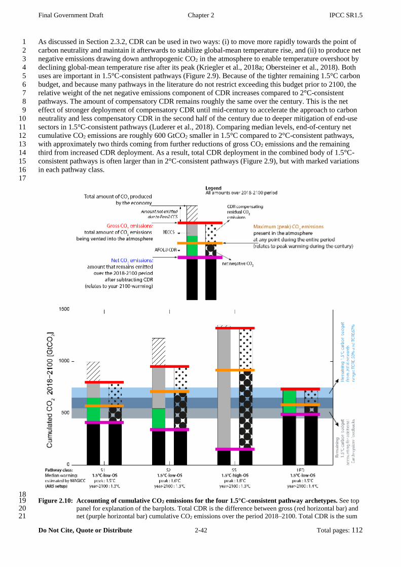
Final Government Draft Chapter 2 IPCC SR1.5
Do Not Cite, Quote or Distribute 2-42 Total pages: 112
As discussed in Section 2.3.2, CDR can be used in two ways: (i) to move more rapidly towards the point of 1
carbon neutrality and maintain it afterwards to stabilize global-mean temperature rise, and (ii) to produce net 2
negative emissions drawing down anthropogenic CO2 in the atmosphere to enable temperature overshoot by 3
declining global-mean temperature rise after its peak (Kriegler et al., 2018a; Obersteiner et al., 2018). Both 4
uses are important in 1.5°C-consistent pathways (Figure 2.9). Because of the tighter remaining 1.5°C carbon 5
budget, and because many pathways in the literature do not restrict exceeding this budget prior to 2100, the 6
relative weight of the net negative emissions component of CDR increases compared to 2°C-consistent 7
pathways. The amount of compensatory CDR remains roughly the same over the century. This is the net 8
effect of stronger deployment of compensatory CDR until mid-century to accelerate the approach to carbon 9
neutrality and less compensatory CDR in the second half of the century due to deeper mitigation of end-use 10
sectors in 1.5°C-consistent pathways (Luderer et al., 2018). Comparing median levels, end-of-century net 11
cumulative CO2 emissions are roughly 600 GtCO2 smaller in 1.5°C compared to 2°C-consistent pathways, 12
with approximately two thirds coming from further reductions of gross CO2 emissions and the remaining 13
third from increased CDR deployment. As a result, total CDR deployment in the combined body of 1.5°C-14
consistent pathways is often larger than in 2°C-consistent pathways (Figure 2.9), but with marked variations 15
in each pathway class. 16
17
18 Figure 2.10: Accounting of cumulative CO2 emissions for the four 1.5°C-consistent pathway archetypes. See top 19
panel for explanation of the barplots. Total CDR is the difference between gross (red horizontal bar) and 20 net (purple horizontal bar) cumulative CO2 emissions over the period 2018–2100. Total CDR is the sum 21
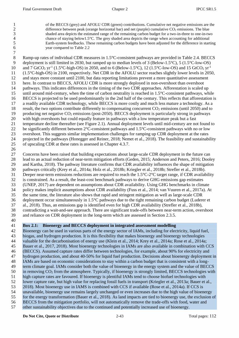
Final Government Draft Chapter 2 IPCC SR1.5
Do Not Cite, Quote or Distribute 2-43 Total pages: 112
of the BECCS (grey) and AFOLU CDR (green) contributions. Cumulative net negative emissions are the 1 difference between peak (orange horizontal bar) and net (purple) cumulative CO2 emissions. The blue 2 shaded area depicts the estimated range of the remaining carbon budget for a two-in-three to one-in-two 3 chance of staying below1.5°C. The grey shaded area depicts the range when accounting for additional 4 Earth-system feedbacks. These remaining carbon budgets have been adjusted for the difference in starting 5 year compared to Table 2.2 6
7 Ramp-up rates of individual CDR measures in 1.5°C-consistent pathways are provided in Table 2.4. BECCS 8
deployment is still limited in 2030, but ramped up to median levels of 3 (Below-1.5°C), 5 (1.5°C-low-OS) 9
and 7 GtCO2 yr-1 (1.5°C-high-OS) in 2050, and to 6 (Below-1.5°C), 12 (1.5°C-low-OS) and 15 GtCO2 yr-1 10
(1.5°C-high-OS) in 2100, respectively. Net CDR in the AFOLU sector reaches slightly lower levels in 2050, 11
and stays more constant until 2100, but data reporting limitations prevent a more quantitative assessment 12
here. In contrast to BECCS, AFOLU CDR is more strongly deployed in non-overshoot than overshoot 13
pathways. This indicates differences in the timing of the two CDR approaches. Afforestation is scaled up 14
until around mid-century, when the time of carbon neutrality is reached in 1.5°C-consistent pathways, while 15
BECCS is projected to be used predominantly in the 2nd half of the century. This reflects that afforestation is 16
a readily available CDR technology, while BECCS is more costly and much less mature a technology. As a 17
result, the two options contribute differently to compensating concurrent CO2 emissions (until 2050) and to 18
producing net negative CO2 emissions (post-2050). BECCS deployment is particularly strong in pathways 19
with high overshoots but could equally feature in pathways with a low temperature peak but a fast 20
temperature decline thereafter (see Figure 2.1). Annual deployment levels until mid-century are not found to 21
be significantly different between 2°C-consistent pathways and 1.5°C-consistent pathways with no or low 22
overshoot. This suggests similar implementation challenges for ramping up CDR deployment at the rates 23
projected in the pathways (Honegger and Reiner, 2018; Nemet et al., 2018). The feasibility and sustainability 24
of upscaling CDR at these rates is assessed in Chapter 4.3.7. 25
26
Concerns have been raised that building expectations about large-scale CDR deployment in the future can 27
lead to an actual reduction of near-term mitigation efforts (Geden, 2015; Anderson and Peters, 2016; Dooley 28
and Kartha, 2018). The pathway literature confirms that CDR availability influences the shape of mitigation 29
pathways critically (Krey et al., 2014a; Holz et al., 2018b; Kriegler et al., 2018b; Strefler et al., 2018b). 30
Deeper near-term emissions reductions are required to reach the 1.5°C-2°C target range, if CDR availability 31
is constrained. As a result, the least-cost benchmark pathways to derive GHG emissions gap estimates 32
(UNEP, 2017) are dependent on assumptions about CDR availability. Using GHG benchmarks in climate 33
policy makes implicit assumptions about CDR availability (Fuss et al., 2014; van Vuuren et al., 2017a). At 34
the same time, the literature also shows that rapid and stringent mitigation as well as large-scale CDR 35
deployment occur simultaneously in 1.5°C pathways due to the tight remaining carbon budget (Luderer et 36
al., 2018). Thus, an emissions gap is identified even for high CDR availability (Strefler et al., 2018b), 37
contradicting a wait-and-see approach. There are significant trade-offs between near-term action, overshoot 38
and reliance on CDR deployment in the long-term which are assessed in Section 2.3.5. 39
40
Box 2.1: Bioenergy and BECCS deployment in integrated assessment modelling 41
Bioenergy can be used in various parts of the energy sector of IAMs, including for electricity, liquid fuel, 42
biogas, and hydrogen production. It is this flexibility that makes bioenergy and bioenergy technologies 43
valuable for the decarbonisation of energy use (Klein et al., 2014; Krey et al., 2014a; Rose et al., 2014a; 44
Bauer et al., 2017, 2018). Most bioenergy technologies in IAMs are also available in combination with CCS 45
(BECCS). Assumed capture rates differ between technologies, for example, about 90% for electricity and 46
hydrogen production, and about 40-50% for liquid fuel production. Decisions about bioenergy deployment in 47
IAMs are based on economic considerations to stay within a carbon budget that is consistent with a long-48
term climate goal. IAMs consider both the value of bioenergy in the energy system and the value of BECCS 49
in removing CO2 from the atmosphere. Typically, if bioenergy is strongly limited, BECCS technologies with 50
high capture rates are favoured. If bioenergy is plentiful IAMs tend to choose biofuel technologies with 51
lower capture rate, but high value for replacing fossil fuels in transport (Kriegler et al., 2013a; Bauer et al., 52
2018). Most bioenergy use in IAMS is combined with CCS if available (Rose et al., 2014a). If CCS is 53
unavailable, bioenergy use remains largely unchanged or even increases due to the high value of bioenergy 54
for the energy transformation (Bauer et al., 2018). As land impacts are tied to bioenergy use, the exclusion of 55
BECCS from the mitigation portfolio, will not automatically remove the trade-offs with food, water and 56
other sustainability objectives due to the continued and potentially increased use of bioenergy. 57
Final Government Draft Chapter 2 IPCC SR1.5
Do Not Cite, Quote or Distribute 2-44 Total pages: 112
1
IAMs assume bioenergy to be supplied mostly from second generation biomass feedstocks such as dedicated 2
cellulosic crops (for example Miscanthus or Poplar) as well as agricultural and forest residues. Detailed 3
process IAMs include land-use models that capture competition for land for different uses (food, feed, fiber, 4
bioenergy, carbon storage, biodiversity protection) under a range of dynamic factors including socio-5
economic drivers, productivity increases in crop and livestock systems, food demand, and land, 6
environmental, biodiversity, and carbon policies. Assumptions about these factors can vary widely between 7
different scenarios (Calvin et al., 2014; Popp et al., 2017; van Vuuren et al., 2018). IAMs capture a number 8
of potential environmental impacts from bioenergy production, in particular indirect land-use change 9
emissions from land conversion and nitrogen and water use for bioenergy production (Kraxner et al., 2013; 10
Bodirsky et al., 2014; Bonsch et al., 2014; Obersteiner et al., 2016; Humpenöder et al., 2017). Especially the 11
impact of bioenergy production on soil degradation is an area of active IAM development and was not 12
comprehensively accounted for in the mitigation pathways assessed in this report (but is, for example, in 13
(Frank et al., 2017)). Whether bioenergy has large adverse impacts on environmental and societal goals 14
depends in large parts on the governance of land use (Haberl et al., 2013; Erb et al., 2016b; Obersteiner et al., 15
2016; Humpenöder et al., 2017). Here IAMs often make idealized assumptions about effective land 16
management such as full protection of the land carbon stock by conservation measures and a global carbon 17
price, respectively, but also variations on these assumptions have been explored (Calvin et al., 2014; Popp et 18
al., 2014a)). 19
20
21
Sustainability implications of CDR deployment in 1.5°C-consistent pathways 22
23
Strong concerns about the sustainability implications of large-scale CDR deployment in deep mitigation 24
pathways have been raised in the literature (Williamson and Bodle, 2016; Boysen et al., 2017b; Dooley and 25
Kartha, 2018; Heck et al., 2018), and a number of important knowledge gaps have been identified (Fuss et 26
al., 2016). An assessment of the literature on implementation constraints and sustainable development 27
implications of CDR measures is provided in Section 4.3.7 and the Cross-chapter Box 7 in Chapter 3. 28
Potential environmental side effects as initial context for the discussion of CDR deployment in 1.5°C-29
consistent pathways are provided in this section. Section 4.3.7 then contrasts CDR deployment in 1.5°C-30
consistent pathways with other branches of literature on limitations of CDR. Integrated modelling aims to 31
explore a range of developments compatible with specific climate goals and often does not include the full 32
set of broader environmental and societal concerns beyond climate change. This has given rise to the concept 33
of sustainable development pathways (van Vuuren et al., 2015) (Cross-Chapter Box 1 in Chapter 1), and 34
there is an increasing body of work to extend integrated modelling to cover a broader range of sustainable 35
development goals (Section 2.6). However, only some of the available 1.5°C-consistent pathways were 36
developed within a larger sustainable development context (Bertram et al., 2018; Grubler et al., 2018; 37
Rogelj et al., 2018; van Vuuren et al., 2018). As discussed in Section 2.3.4.1, those pathways are 38
characterized by low energy and/or food demand effectively limiting fossil-fuel substitution and alleviating 39
land competition, respectively. They also include regulatory policies for deepening early action and ensuring 40
environmental protection (Bertram et al., 2018). Overall sustainability implications of 1.5°C-consistent 41
pathways are assessed in Section 2.5.3 and Section 5.4. 42
43
Individual CDR measures have different characteristics and therefore would carry different risks for their 44
sustainable deployment at scale (Smith et al., 2015). Terrestrial CDR measures, BECCS and enhanced 45
weathering of rock powder distributed on agricultural lands require land. Those land-based measures could 46
have substantial impacts on environmental services and ecosystems (Smith and Torn, 2013; Boysen et al., 47
2016; Heck et al., 2016; Krause et al., 2017) (Cross-Chapter Box 7 in Chapter 3). Measures like afforestation 48
and bioenergy with and without CCS that directly compete with other land uses could have significant 49
impacts on agricultural and food systems (Creutzig et al., 2012, 2015; Calvin et al., 2014; Popp et al., 2014b, 50
2017; Kreidenweis et al., 2016; Boysen et al., 2017a; Frank et al., 2017; Humpenöder et al., 2017; 51
Stevanović et al., 2017; Strapasson et al., 2017). BECCS using dedicated bioenergy crops could substantially 52
increase agricultural water demand (Bonsch et al., 2014; Séférian et al., 2018) and nitrogen fertilizer use 53
(Bodirsky et al., 2014). DACCS and BECCS rely on CCS and would require safe storage space in geological 54
formations, including management of leakage risks (Pawar et al., 2015) and induced seismicity (Nicol et al., 55
2013). Some approaches like DACCS have high energy demand (Socolow et al., 2011). Most of the CDR 56
measures currently discussed could have significant impacts on either land, energy, water, or nutrients if 57

Final Government Draft Chapter 2 IPCC SR1.5
Do Not Cite, Quote or Distribute 2-45 Total pages: 112
deployed at scale (Smith et al., 2015). However, actual trade-offs depend on a multitude factors (Haberl et 1
al., 2011; Erb et al., 2012; Humpenöder et al., 2017), including the modalities of CDR deployment (e.g., on 2
marginal vs. productive land) (Bauer et al., 2018), socio-economic developments (Popp et al., 2017), dietary 3
choices (Stehfest et al., 2009; Popp et al., 2010; van Sluisveld et al., 2016; Weindl et al., 2017; van Vuuren et 4
al., 2018), yield increases, livestock productivity and other advances in agricultural technology (Havlik et al., 5
2013; Valin et al., 2013; Havlík et al., 2014; Weindl et al., 2015; Erb et al., 2016b), land policies (Schmitz et 6
al., 2012; Calvin et al., 2014; Popp et al., 2014a) and governance of land use (Unruh, 2011; Buck, 2016; 7
Honegger and Reiner, 2018). 8
9
Figure 2.11 shows the land requirements for BECCS and afforestation in the selected 1.5°C-consistent 10
pathway archetypes, including the LED (Grubler et al., 2018) and S1 pathways (Fujimori, 2017; Rogelj et 11
al., 2018) following a sustainable development paradigm. As discussed, these land-use patterns are heavily 12
influenced by assumptions about, inter alia, future population levels, crop yields, livestock production 13
systems, and food and livestock demand, which all vary between the pathways (Popp et al., 2017) (Section 14
2.3.1.1). In pathways that allow for large-scale afforestation in addition to BECCS, land demand for 15
afforestation can be larger than for BECCS (Humpenöder et al., 2014). This follows from the assumption in 16
the modelled pathways that, unlike bioenergy crops, forests are not harvested to allow unabated carbon 17
storage on the same patch of land. If wood harvest and subsequent processing or burial are taken into 18
account, this finding can change. There are also synergies between the various uses of land, which are not 19
reflected in the depicted pathways. Trees can grow on agricultural land (Zomer et al., 2016) and harvested 20
wood can be used with BECCS and pyrolysis systems (Werner et al., 2018). The pathways show a very 21
substantial land demand for the two CDR measures combined, up to the magnitude of the current global 22
cropland area. This is achieved in IAMs in particular by a conversion of pasture land freed by intensification 23
of livestock production systems, pasture intensification and/or demand changes (Weindl et al., 2017), and to 24
more limited extent cropland for food production, as well as expansion into natural land. However, pursuing 25
such large scale changes in land use would pose significant food supply, environmental and governance 26
challenges, concerning both land management and tenure (Unruh, 2011; Erb et al., 2012, 2016b; Haberl et 27
al., 2013; Haberl, 2015; Buck, 2016), particularly if synergies between land uses, the relevance of dietary 28
changes for reducing land demand, and co-benefits with other sustainable development objectives are not 29
fully recognized. A general discussion of the land-use transformation in 1.5°C-consistent pathways is 30
provided in Section 2.4.4. 31
32
An important consideration for CDR which moves carbon from the atmosphere to the geological, oceanic or 33
terrestrial carbon pools is the permanence of carbon stored in these different pools (Matthews and Caldeira, 34
2008; NRC, 2015; Fuss et al., 2016; Jones et al., 2016) (see also Section 4.3.7 for a discussion). Terrestrial 35
carbon can be returned to the atmosphere on decadal timescales by a variety of mechanisms such as soil 36
degradation, forest pest outbreaks and forest fires, and therefore requires careful consideration of policy 37
frameworks to manage carbon storage, e.g., in forests (Gren and Aklilu, 2016). There are similar concerns 38
about outgassing of CO2 from ocean storage (Herzog et al., 2003), unless it is transformed to a substance that 39
does not easily exchange with the atmosphere, e.g., ocean alkalinity or buried marine biomass (Rau, 2011). 40
Understanding of the assessment and management of the potential risk of CO2 release from geological 41
storage of CO2 has improved since the IPCC Special Report on Carbon Dioxide Capture and Storage (IPCC, 42
2005) with experience and the development of management practices in geological storage projects, 43
including risk management to prevent sustentative leakage (Pawar et al., 2015). Estimates of leakage risk 44
have been updated to include scenarios of unregulated drilling and limited wellbore integrity (Choi et al., 45
2013), finding ca. 70% of stored CO2 still retained after 10,000 years in these circumstances (Alcalde et al., 46
2018). The literature on the potential environmental impacts from the leakage of CO2 – and approaches to 47
minimize these impacts should a leak occur – has also grown and is reviewed by Jones et al. (2015). To the 48
extent non-permanence of terrestrial and geological carbon storage is driven by socio-economic and political 49
factors, it has parallels to questions of fossil-fuel reservoirs remaining in the ground (Scott et al., 2015). 50
51
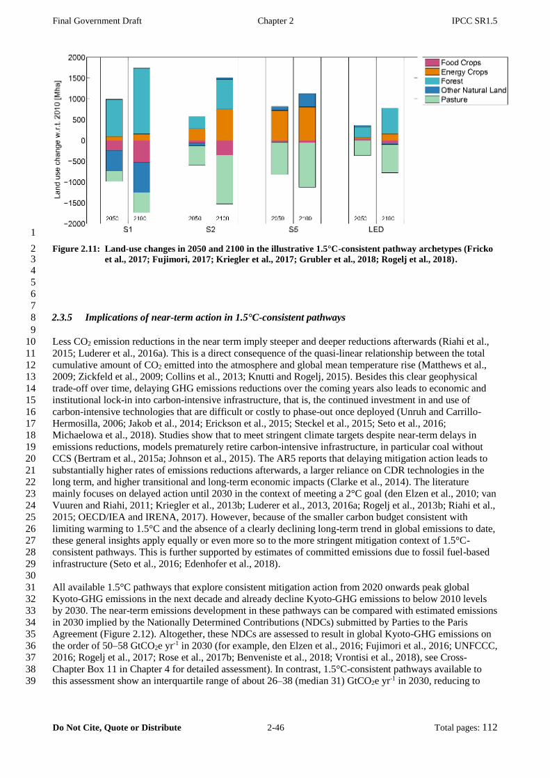
Final Government Draft Chapter 2 IPCC SR1.5
Do Not Cite, Quote or Distribute 2-46 Total pages: 112
1
Figure 2.11: Land-use changes in 2050 and 2100 in the illustrative 1.5°C-consistent pathway archetypes (Fricko 2 et al., 2017; Fujimori, 2017; Kriegler et al., 2017; Grubler et al., 2018; Rogelj et al., 2018). 3
4
5
6
7
2.3.5 Implications of near-term action in 1.5°C-consistent pathways 8
9
Less CO2 emission reductions in the near term imply steeper and deeper reductions afterwards (Riahi et al., 10
2015; Luderer et al., 2016a). This is a direct consequence of the quasi-linear relationship between the total 11
cumulative amount of CO2 emitted into the atmosphere and global mean temperature rise (Matthews et al., 12
2009; Zickfeld et al., 2009; Collins et al., 2013; Knutti and Rogelj, 2015). Besides this clear geophysical 13
trade-off over time, delaying GHG emissions reductions over the coming years also leads to economic and 14
institutional lock-in into carbon-intensive infrastructure, that is, the continued investment in and use of 15
carbon-intensive technologies that are difficult or costly to phase-out once deployed (Unruh and Carrillo-16
Hermosilla, 2006; Jakob et al., 2014; Erickson et al., 2015; Steckel et al., 2015; Seto et al., 2016; 17
Michaelowa et al., 2018). Studies show that to meet stringent climate targets despite near-term delays in 18
emissions reductions, models prematurely retire carbon-intensive infrastructure, in particular coal without 19
CCS (Bertram et al., 2015a; Johnson et al., 2015). The AR5 reports that delaying mitigation action leads to 20
substantially higher rates of emissions reductions afterwards, a larger reliance on CDR technologies in the 21
long term, and higher transitional and long-term economic impacts (Clarke et al., 2014). The literature 22
mainly focuses on delayed action until 2030 in the context of meeting a 2°C goal (den Elzen et al., 2010; van 23
Vuuren and Riahi, 2011; Kriegler et al., 2013b; Luderer et al., 2013, 2016a; Rogelj et al., 2013b; Riahi et al., 24
2015; OECD/IEA and IRENA, 2017). However, because of the smaller carbon budget consistent with 25
limiting warming to 1.5°C and the absence of a clearly declining long-term trend in global emissions to date, 26
these general insights apply equally or even more so to the more stringent mitigation context of 1.5°C-27
consistent pathways. This is further supported by estimates of committed emissions due to fossil fuel-based 28
infrastructure (Seto et al., 2016; Edenhofer et al., 2018). 29
30
All available 1.5°C pathways that explore consistent mitigation action from 2020 onwards peak global 31
Kyoto-GHG emissions in the next decade and already decline Kyoto-GHG emissions to below 2010 levels 32
by 2030. The near-term emissions development in these pathways can be compared with estimated emissions 33
in 2030 implied by the Nationally Determined Contributions (NDCs) submitted by Parties to the Paris 34
Agreement (Figure 2.12). Altogether, these NDCs are assessed to result in global Kyoto-GHG emissions on 35
the order of 50–58 GtCO2e yr-1 in 2030 (for example, den Elzen et al., 2016; Fujimori et al., 2016; UNFCCC, 36
2016; Rogelj et al., 2017; Rose et al., 2017b; Benveniste et al., 2018; Vrontisi et al., 2018), see Cross-37
Chapter Box 11 in Chapter 4 for detailed assessment). In contrast, 1.5°C-consistent pathways available to 38
this assessment show an interquartile range of about 26–38 (median 31) GtCO2e yr-1 in 2030, reducing to 39

Final Government Draft Chapter 2 IPCC SR1.5
Do Not Cite, Quote or Distribute 2-47 Total pages: 112
26–31 (median 28) GtCO2e yr-1 if only pathways with low overshoot are taken into account5, and still lower 1
if pathways without overshoot are considered (Table 2.4, Section 2.3.3). Published estimates of the 2
emissions gap between conditional NDCs and 1.5°C-consistent pathways in 2030 range from 16 (14–22) 3
GtCO2e yr-1 (UNEP, 2017) for a greater than one-in-to chance of limiting warming below 1.5°C in 2100 to 4
25 (19–29) GtCO2e yr-1 (Vrontisi et al., 2018) for a greater than two-in-three chance of meeting the 1.5°C 5
limit. 6
7
The later emissions peak and decline, the more CO2 will have accumulated in the atmosphere. Peak 8
cumulated CO2 emissions and consequently also peak temperatures increase with 2030 emissions levels 9
(Figure 2.12). Current NDCs (Cross-Chapter Box 11 in Chapter 4) are estimated to lead to CO2 emissions of 10
about 400–560 GtCO2 from 2018 to 2030 (Rogelj et al., 2016a). Available 1.5°C- and 2°C-consistent 11
pathways with 2030 emissions in the range estimated for the NDCs rely on an assumed swift and widespread 12
deployment of CDR after 2030, and show peak cumulative CO2 emissions from 2018 of about 800–1000 13
GtCO2, above the remaining carbon budget for a one-in-two chance of remaining below 1.5°C. These 14
emissions reflect that no pathway is able to project a phase out of CO2 emissions starting from year-2030 15
NDC levels of about 40 GtCO2 yr-1 (Fawcett et al., 2015; Rogelj et al., 2016a) to net zero in less than ca. 15 16
years. Based on the implied emissions until 2030, the high challenges of the assumed post-2030 transition, 17
and the assessment of carbon budgets in Section 2.2.2, global warming is assessed to exceed 1.5°C if 18
emissions stay at the levels implied by the NDCs until 2030 (Figure 2.12). The chances of remaining below 19
1.5°C in these circumstances remain conditional upon geophysical properties that are uncertain, but these 20
Earth system response uncertainties would have to serendipitously align beyond current median estimates in 21
order for current NDCs to become consistent with limiting warming to 1.5°C. 22
23
24 Figure 2.12: Median global warming estimated by MAGICC (left panel) and peak cumulative CO2 emissions 25
(right panel) in 1.5°C-consistent pathways in the SR1.5 scenario database as a function of CO2-26 equivalent emissions (based on AR4 GWP-100) of Kyoto-GHGs in 2030. Pathways that were forced 27 to go through the NDCs or a similarly high emissions point in 2030 by design are highlighted by yellow 28 marker edges (see caption of Figure 2.13 and text for further details on the design of these pathways). The 29 NDC range of global Kyoto-GHG emissions in 2030 assessed in Cross-Chapter Box 11 in Chapter 4 is 30 shown by black dotted lines (adjusted to AR4 GWPs for comparison). As a second line of evidence, peak 31 cumulative CO2 emissions derived from a 1.5°C pathway sensitivity analysis (Kriegler et al., 2018a) are 32 shown by grey circles in the right-hand panel. Numbers show gross fossil-fuel and industry emissions of 33
5: Note that aggregated Kyoto-GHG emissions implied by the NDCs from Cross-Chapter Box 4.3 and Kyoto-GHG ranges from the pathway classes in
Chapter 2 are only approximately comparable, because this chapter applies GWP-100 values from the IPCC Fourth Assessment Report while the NDC Cross-Chapter Box 4.3 applies GWP-100 values from the IPCC Second Assessment Report. At a global scale, switching between GWP-100 values of
the Second to the Fourth IPCC Assessment Report would result in an increase in estimated aggregated Kyoto-GHG emissions of about no more than
3% in 2030 (UNFCCC, 2016).

Final Government Draft Chapter 2 IPCC SR1.5
Do Not Cite, Quote or Distribute 2-48 Total pages: 112
the sensitivity cases increased by assumptions about the contributions from AFOLU (5 GtCO2 yr-1 until 1 2020, followed by a linear phase out until 2040) and non-CO2 Kyoto-GHGs (median non-CO2 2 contribution from 1.5°C-consistent pathways available in the database: 10 GtCO2e yr-1 in 2030), and 3 reduced by assumptions about CDR deployment until the time of net zero CO2 emissions (limiting case 4 for CDR deployment assumed in (Kriegler et al., 2018a) (logistic growth to 1, 4, 10 GtCO2 yr-1 in 2030, 5 2040, and 2050, respectively, leading to approx. 100 GtCO2 CDR by mid-century). 6
7
It is unclear whether following NDCs until 2030 would still allow global mean temperature to return to 8
1.5°C by 2100 after a temporary overshoot, due to the uncertainty associated with the Earth system response 9
to net negative emissions after a peak (Section 2.2). Available IAM studies are working with reduced-form 10
carbon cycle-climate models like MAGICC which assume a largely symmetric Earth-system response to 11
positive and net negative CO2 emissions. The IAM findings on returning warming to 1.5°C from NDCs after 12
a temporary temperature overshoot are hence all conditional on this assumption. Two types of pathways with 13
1.5°C-consistent action starting in 2030 have been considered in the literature (Luderer et al., 2018) (Figure 14
2.13): pathways aiming to obtain the same end-of-century carbon budget despite higher emissions until 2030, 15
and pathways assuming the same mitigation stringency after 2030 (approximated by using the same global 16
price of emissions as found in least-cost pathways starting from 2020). An IAM comparison study found 17
increasing challenges to implement pathways with the same end-of-century 1.5°C-consistent carbon budgets 18
after following NDCs until 2030 (ADVANCE) (Luderer et al., 2018). The majority of model experiments 19
(four out of seven) failed to produce NDC pathways that would return cumulative CO2 emissions over the 20
2016–2100 period to 200 GtCO2, indicating limitations to the availability and timing of CDR. The few such 21
pathways that were identified show highly disruptive features in 2030 (including abrupt transitions from 22
moderate to very large emissions reduction and low carbon energy deployment rates) indicating a high risk 23
that the required post-2030 transformations are too steep and abrupt to be achieved by the mitigation 24
measures in the models (high confidence). NDC pathways aiming for a cumulative 2016–2100 CO2 25
emissions budget of 800 GtCO2 were more readily obtained (Luderer et al., 2018), and some were classified 26
as 1.5°C-high-OS pathways in this assessment (Section 2.1). 27
28
NDC pathways that apply a post-2030 price of emissions after 2030 as found in least-cost pathways starting 29
from 2020 show infrastructural carbon lock-in as a result of following NDCs instead of least-cost action until 30
2030. A key finding is that carbon lock-ins persist long after 2030, with the majority of additional CO2 31
emissions occurring during the 2030–2050 period. Luderer et al. (2018) find 90 (80–120) GtCO2 additional 32
emissions until 2030, growing to 240 (190–260) GtCO2 by 2050 and 290 (200–200) GtCO2 by 2100. As a 33
result, peak warming is about 0.2°C higher and not all of the modelled pathways return warming to 1.5°C by 34
the end of the century. There is a four sided trade-off between (i) near-term ambition, (ii) degree of 35
overshoot, (iii) transitional challenges during the 2030–2050 period, and (iv) the amount of CDR deployment 36
required during the century (Figure 2.13) (Holz et al., 2018b; Strefler et al., 2018b). Transition challenges, 37
overshoot, and CDR requirements can be significantly reduced if global emissions peak before 2030 and fall 38
below levels in line with current NDCs by 2030. For example, Strefler et al. (2018b) find that CDR 39
deployment levels in the second half of the century can be halved in 1.5°C-consistent pathways with similar 40
CO2 emissions reductions rates during the 2030–2050 period if CO2 emissions by 2030 are reduced by an 41
additional 30% compared to NDC levels. Kriegler et al. (2018b) investigate a global roll out of selected 42
regulatory policies and moderate carbon pricing policies. They show that additional reductions of ca. 43
10 GtCO2e yr-1 can be achieved in 2030 compared to the current NDCs. Such 20% reduction of year-2030 44
emissions compared to current NDCs would effectively lower the disruptiveness of post-2030 action. 45
Strengthening of short-term policies in deep mitigation pathways has hence been identified as bridging 46
options to keep the Paris climate goals within reach (Bertram et al., 2015b; IEA, 2015a; Spencer et al., 2015; 47
Kriegler et al., 2018b). 48
49
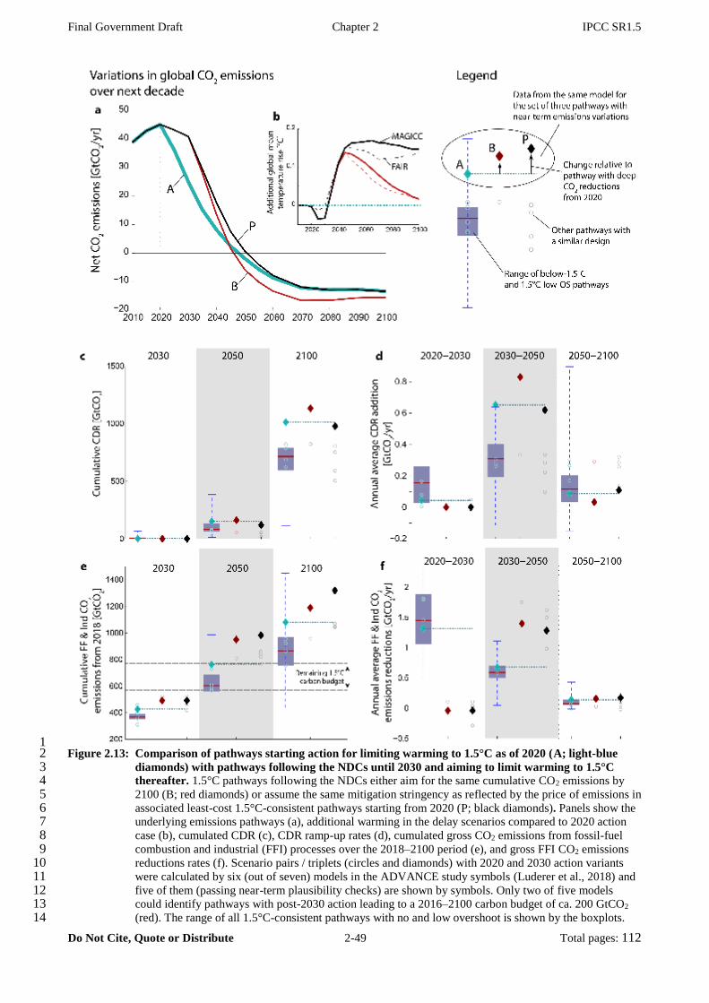
Final Government Draft Chapter 2 IPCC SR1.5
Do Not Cite, Quote or Distribute 2-49 Total pages: 112
1 Figure 2.13: Comparison of pathways starting action for limiting warming to 1.5°C as of 2020 (A; light-blue 2
diamonds) with pathways following the NDCs until 2030 and aiming to limit warming to 1.5°C 3 thereafter. 1.5°C pathways following the NDCs either aim for the same cumulative CO2 emissions by 4 2100 (B; red diamonds) or assume the same mitigation stringency as reflected by the price of emissions in 5 associated least-cost 1.5°C-consistent pathways starting from 2020 (P; black diamonds). Panels show the 6 underlying emissions pathways (a), additional warming in the delay scenarios compared to 2020 action 7 case (b), cumulated CDR (c), CDR ramp-up rates (d), cumulated gross CO2 emissions from fossil-fuel 8 combustion and industrial (FFI) processes over the 2018–2100 period (e), and gross FFI CO2 emissions 9 reductions rates (f). Scenario pairs / triplets (circles and diamonds) with 2020 and 2030 action variants 10 were calculated by six (out of seven) models in the ADVANCE study symbols (Luderer et al., 2018) and 11 five of them (passing near-term plausibility checks) are shown by symbols. Only two of five models 12 could identify pathways with post-2030 action leading to a 2016–2100 carbon budget of ca. 200 GtCO2 13 (red). The range of all 1.5°C-consistent pathways with no and low overshoot is shown by the boxplots. 14

Final Government Draft Chapter 2 IPCC SR1.5
Do Not Cite, Quote or Distribute 2-50 Total pages: 112
2.4 Disentangling the whole-system transformation 1
2
Mitigation pathways map out prospective transformations of the energy, land and economic systems over 3
this century (Clarke et al., 2014). There is a diversity of potential pathways consistent with 1.5°C, yet they 4
share some key characteristics summarized in Table 2.5. To explore characteristics of 1.5°C pathways in 5
greater detail, this section focuses on changes in energy supply and demand, and changes in the AFOLU 6
sector. 7
8
9 Table 2.5: Overview of key characteristics of 1.5°C pathways. 10
11 1.5°C pathway characteristic Supporting information Reference
Rapid and profound near-term decarbonisation of energy supply
Strong upscaling of renewables and sustainable biomass and reduction of unabated (no CCS) fossil fuels, along with the rapid deployment of CCS lead to a zero-emission energy supply system by mid-century.
Section 2.4.1 Section 2.4.2
Greater mitigation efforts on the demand side
All end-use sectors show marked demand reductions beyond the reductions projected for 2°C pathways. Demand reductions from IAMs for 2030 and 2050 lie within the potential assessed by detailed sectorial bottom-up assessments.
Section 2.4.3
Switching from fossil fuels to electricity in end-use sectors
Both in the transport and the residential sector, electricity covers marked larger shares of total demand by mid-century.
Section 2.4.3.2 Section 2.4.3.3
Comprehensive emission reductions are implemented in the coming decade
Virtually all 1.5°C-consistent pathways decline net annual CO2 emissions between 2020 and 2030, reaching carbon neutrality around mid-century. Below-1.5°C and 1.5°C-low-OS show maximum net CO2 emissions in 2030 of 18 and 28 GtCO2 yr-1, respectively. GHG emissions in these scenarios are not higher than 34 GtCO2e yr–1 in 2030.
Section 2.3.4
Additional reductions, on top of reductions from both CO2 and non-CO2 required for 2°C, are mainly from CO2
Both CO2 and the non-CO2 GHGs and aerosols are strongly reduced by 2030 and until 2050 in 1.5°C pathways. The greatest difference to 2°C pathways, however, lies in additional reductions of CO2, as the non-CO2 mitigation potential that is currently included in integrated pathways is mostly already fully deployed for reaching a 2°C pathway.
Section 2.3.1.2
Considerable shifts in investment patterns
Low-carbon investments in the energy supply side (energy production and refineries) are projected to average 1.6-3.8 trillion 2010USD yr–1 globally to 2050. Investments in fossil fuels decline, with investments in unabated coal halted by 2030 in most available 1.5°C-consistent projections, while the literature is less conclusive for investments in unabated gas and oil. Energy demand investments are a critical factor for which total estimates are uncertain.
Section 2.5.2
Options are available to align 1.5°C pathways with sustainable development
Synergies can be maximized, and risks of trade-offs limited or avoided through an informed choice of mitigation strategies. Particularly pathways that focus on a lowering of demand show many synergies and few trade-offs.
Section 2.5.3
CDR at scale before mid-century
By 2050, 1.5°C pathways project deployment of BECCS at a scale of 3–7 GtCO2yr–1 (range of medians across 1.5°C pathway classes), depending on the level of energy demand reductions and mitigation in other sectors. Some 1.5°C pathways are available that do not use BECCS, but only focus terrestrial CDR in the AFOLU sector.
Section 2.3.3, 2.3.4.1
12 13
2.4.1 Energy System Transformation 14
15
The energy system links energy supply (Section 2.4.2) with energy demand (Section 2.4.3) through final 16
energy carriers including electricity and liquid, solid or gaseous fuels that are tailored to their end-uses. To 17
chart energy-system transformations in mitigation pathways, four macro-level decarbonisation indicators 18
associated with final energy are useful: limits to the increase of final energy demand, reductions in the 19
carbon intensity of electricity, increases in the share of final energy provided by electricity, and reductions in 20
the carbon intensity of final energy other than electricity (referred to in this section as the carbon intensity of 21
the residual fuel mix). Figure 2.14 shows changes of these four indicators for the pathways in the scenario 22
database (Section 2.1.3 and Supplementary Material 2.SM.1.3) for 1.5°C and 2°C pathways (Table 2.1). 23
24
Pathways in both the 1.5°C and 2°C classes (Figure 2.14) generally show rapid transitions until mid-century 25

Final Government Draft Chapter 2 IPCC SR1.5
Do Not Cite, Quote or Distribute 2-51 Total pages: 112
with a sustained but slower evolution thereafter. Both show an increasing share of electricity accompanied 1
by a rapid decline in the carbon intensity of electricity. Both also show a generally slower decline in the 2
carbon intensity of the residual fuel mix, which arises from the decarbonisation of liquids, gases and solids 3
provided to industry, residential and commercial activities, and the transport sector. 4
5
The largest differences between 1.5°C and 2°C pathways are seen in the first half of the century (Figure 6
2.14), where 1.5°C pathways generally show lower energy demand, a faster electrification of energy end-use, 7
and a faster decarbonisation of the carbon intensity of electricity and the residual fuel mix. There are very 8
few pathways in the Below-1.5°C class (Figure 2.14). Those scenarios that are available, however, show a 9
faster decline in the carbon intensity of electricity generation and residual fuel mix by 2030 than most 10
pathways that are projected to temporarily overshoot 1.5°C and return by 2100 (or 2°C pathways), and also 11
appear to distinguish themselves already by 2030 by reductions in final energy demand and an increased 12
electricity share (Figure 2.14). 13
14 15
Figure 2.14: Decomposition of transformation pathways into energy demand (top left), carbon intensity of 16
electricity (top right), the electricity share in final energy (bottom left), and the carbon intensity of 17 the residual (non-electricity) fuel mix (bottom right). Boxplots show median, interquartile range and 18 full range of pathways. Pathway temperature classes (Table 2.1) and illustrative pathway archetypes are 19 indicated in the legend. Values following the class labels give the number of available pathways in each 20 class. 21
22 23
2.4.2 Energy supply 24
25
Several energy supply characteristics are evident in 1.5°C pathways assessed in this section: i) growth in the 26
share of energy derived from low carbon-emitting sources (including renewables, nuclear, and fossil fuel 27
with CCS) and a decline in the overall share of fossil fuels without CCS (Section 2.4.2.1), ii) rapid decline in 28
the carbon intensity of electricity generation simultaneous with further electrification of energy end-use 29
(Section 2.4.2.2), and iii) the growth in the use of CCS applied to fossil and biomass carbon in most 1.5°C 30
pathways (Section 2.4.2.3). 31
32
33
Evolution of primary energy contributions over time 34
35
By mid-century, the majority of primary energy comes from non-fossil-fuels (i.e., renewables and nuclear 36

Final Government Draft Chapter 2 IPCC SR1.5
Do Not Cite, Quote or Distribute 2-52 Total pages: 112
energy) in most 1.5°C pathways (Table 2.6). Figure 2.15 shows the evolution of primary energy supply over 1
this century across 1.5°C pathways, and in detail for the four illustrative pathway archetypes highlighted in 2
this chapter. Note that this section reports primary energy using the direct equivalent method on a lower 3
heating values basis (Bruckner et al., 2014). 4
5
Renewable energy (including biomass, hydro, solar, wind, and geothermal) increases across all 1.5°C 6
pathways with the renewable energy share of primary energy reaching 28–88% in 2050 (Table 2.6) with an 7
interquartile range of 49–67%. The magnitude and split between bioenergy, wind, solar, and hydro differ 8
between pathways, as can be seen in the illustrative pathway archetypes in Figure 2.15. Bioenergy is a major 9
supplier of primary energy, contributing to both electricity and other forms of final energy such as liquid 10
fuels for transportation (Bauer et al., 2018). In 1.5°C pathways, there is a significant growth in bioenergy 11
used in combination with CCS for pathways where it is included (Figure 2.15). 12
13
Nuclear power increases its share in most 1.5°C pathways by 2050, but in some pathways both the absolute 14
capacity and share of power from nuclear generators declines (Table 2.15). There are large differences in 15
nuclear power between models and across pathways (Kim et al., 2014; Rogelj et al., 2018). One of the 16
reasons for this variation is that the future deployment of nuclear can be constrained by societal preferences 17
assumed in narratives underlying the pathways (O’Neill et al., 2017; van Vuuren et al., 2017b). Some 1.5°C 18
pathways no longer see a role for nuclear fission by the end of the century, while others project over 200 EJ 19
yr–1 of nuclear power in 2100 (Figure 2.15). 20
21
The share of primary energy provided by total fossil fuels decreases from 2020 to 2050 in all 1.5°C 22
pathways, however, trends for oil, gas and coal differ (Table 2.6). By 2050, the share of primary energy from 23
coal decreases to 0–13% across 1.5°C pathways with an interquartile range of 1–7%. From 2020 to 2050 the 24
primary energy supplied by oil changes by –93 to +6% (interquartile range –75 to –32%); natural gas 25
changes by –88 to +99% (interquartile range –60 to –13%), with varying levels of CCS. Pathways with 26
higher use of coal and gas tend to deploy CCS to control their carbon emissions (see Section 2.4.2.3). As the 27
energy transition is accelerated by several decades in 1.5°C pathways compared to 2°C pathways, residual 28
fossil-fuel use (i.e., fossil fuels not used for electricity generation) without CCS is generally lower in 2050 29
than in 2°C pathways, while combined hydro, solar, and wind power deployment is generally higher than in 30
2°C pathways (Figure 2.15). 31
32
In addition to the 1.5°C pathways included in the scenario database (Supplementary Material 2.SM.1.3), 33
there are other analyses in the literature including, for example, sector-based analyses of energy demand and 34
supply options. Even though not necessarily developed in the context of the 1.5°C target, they explore in 35
greater detail some options for deep reductions in GHG emissions. For example, there are analyses of 36
transition to up to 100% renewable energy by 2050 (Creutzig et al., 2017; Jacobson et al., 2017), which 37
describe what is entailed for a renewable energy share largely from solar and wind (and electrification) that 38
is above the range of 1.5°C pathways available in the database, although there have been challenges to the 39
assumptions used in high renewable analyses (e.g., Clack et al., 2017). There are also analyses that result in a 40
large role for nuclear energy in mitigation of GHGs (Hong et al., 2015; Berger et al., 2017a, 2017b; Xiao and 41
Jiang, 2017). BECCS could also contribute a larger share, but faces challenges related to its land use and 42
impact on food supply (Burns and Nicholson, 2017) (assessed in greater detail in Sections 2.3.4.2, 4.3.7 and 43
5.4). These analyses could, provided their assumptions prove plausible, expand the range of 1.5°C pathways. 44
45
In summary, the share of primary energy from renewables increases while that from coal decreases across 46
1.5°C pathways (high confidence). This statement is true for all 1.5°C pathways in the scenario database and 47
associated literature (Supplementary Material 2.SM.1.3), and is consistent with the additional studies 48
mentioned above, an increase in energy supply from lower-carbon-intensity energy supply, and a decrease in 49
energy supply from higher-carbon-intensity energy supply. 50
51
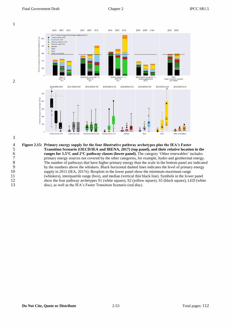
Final Government Draft Chapter 2 IPCC SR1.5
Do Not Cite, Quote or Distribute 2-53 Total pages: 112
1
2
3
Figure 2.15: Primary energy supply for the four illustrative pathway archetypes plus the IEA’s Faster 4 Transition Scenario (OECD/IEA and IRENA, 2017) (top panel), and their relative location in the 5 ranges for 1.5°C and 2°C pathway classes (lower panel). The category ‘Other renewables’ includes 6 primary energy sources not covered by the other categories, for example, hydro and geothermal energy. 7 The number of pathways that have higher primary energy than the scale in the bottom panel are indicated 8 by the numbers above the whiskers. Black horizontal dashed lines indicates the level of primary energy 9 supply in 2015 (IEA, 2017e). Boxplots in the lower panel show the minimum-maximum range 10 (whiskers), interquartile range (box), and median (vertical thin black line). Symbols in the lower panel 11 show the four pathway archetypes S1 (white square), S2 (yellow square), S5 (black square), LED (white 12 disc), as well as the IEA’s Faster Transition Scenario (red disc). 13

Final Government Draft Chapter 2 IPCC SR1.5
Do Not Cite, Quote or Distribute 2-54 Total pages: 112
1
2 Table 2.6: Global primary energy supply of 1.5°C pathways from the scenario database (Supplementary Material 2.SM.1.3). Values given for the median (maximum, 3
minimum) across the full range of 85 available 1.5°C pathways. Growth Factor = [(primary energy supply in 2050)/(primary energy supply in 2020) – 1]. 4 5
Primary energy supply [EJ] Share of primary energy [%] Growth Factor 2020 2030 2050 2020 2050 2020-2050
total primary 582.12 (636.98, 483.22) 502.81 (749.05, 237.37) 580.78 (1012.50, 289.02) 0.03 (0.59, -0.51)
renewables 87.70 (101.60, 60.16) 139.48 (203.90, 87.75) 293.80 (584.78, 176.77) 15.03 (20.39, 10.60) 60.80 (87.89, 28.47) 2.62 (6.71, 0.91) biomass 61.35 (73.03, 40.54) 75.28 (113.02, 44.42) 154.13 (311.72, 40.36) 10.27 (14.23, 7.14) 26.38 (54.10, 10.29) 1.71 (5.56, -0.42) non-biomass 26.35 (36.58, 17.60) 61.60 (114.41, 25.79) 157.37 (409.94, 53.79) 4.40 (7.19, 2.84) 28.60 (61.61, 9.87) 4.63 (13.46, 1.38)
nuclear 10.93 (18.55, 8.52) 16.22 (41.73, 6.80) 24.48 (115.80, 3.09) 1.97 (3.37, 1.45) 4.22 (13.60, 0.43) 1.34 (7.22, -0.64)
fossil 493.44 (638.04, 376.30) 347.62 (605.68, 70.14) 199.63 (608.39, 43.87) 83.56 (114.75, 77.73) 33.58 (74.63, 7.70) -0.58 (0.12, -0.91) coal 147.09 (193.55, 83.23) 49.46 (176.99, 5.97) 23.84 (134.69, 0.36) 25.72 (30.82, 17.19) 4.99 (13.30, 0.05) -0.85 (-0.30, -1.00) gas 135.58 (169.50, 105.01) 127.99 (208.55, 17.30) 88.97 (265.66, 14.92) 23.28 (28.39, 18.09) 13.46 (34.83, 2.80) -0.37 (0.99, -0.88) oil 195.02 (245.15, 151.02) 175.69 (319.80, 38.94) 93.48 (208.04, 15.07) 33.79 (42.24, 28.07) 16.22 (27.30, 2.89) -0.54 (0.06, -0.93)
6
7
8 Table 2.7: Global electricity generation of 1.5°C pathways from the scenarios database (Supplementary Material 2.SM.1.3). Values given for the median (maximum, 9
minimum) values across the full range across 89 available 1.5°C pathways. Growth Factor = [(primary energy supply in 2050)/(primary energy supply in 2020) – 1]. 10 11
Electricty generation [EJ] Share of electricity generation [%] Growth Factor 2020 2030 2050 2020 2050 2020-2050
total electricity 100.09 (113.98, 83.53) 120.01 (177.51, 81.28) 224.78 (363.10, 126.96) 1.31 (2.55, 0.28)
renewables 26.38 (41.80, 18.26) 59.50 (111.70, 30.06) 153.72 (324.26, 84.69) 27.95 (41.84, 17.38) 77.52 (96.65, 35.58) 5.08 (10.88, 2.37) biomass 1.52 (7.00, 0.66) 3.55 (11.96, 0.79) 16.32 (40.32, 0.21) 1.55 (7.30, 0.63) 8.02 (30.28, 0.08) 6.53 (38.14, -0.93) non-biomass 24.48 (35.72, 17.60) 55.68 (101.90, 25.79) 136.40 (323.91, 53.79) 25.00 (40.43, 16.75) 66.75 (96.46, 27.51) 4.75 (10.64, 1.38)
nuclear 10.84 (18.55, 8.52) 15.49 (41.73, 6.80) 22.64 (115.80, 3.09) 10.91 (18.34, 8.62) 8.87 (39.61, 1.02) 1.21 (7.22, -0.64)
fossil 61.35 (76.76, 39.48) 38.41 (87.54, 2.25) 14.10 (118.12, 0.00) 61.55 (71.03, 47.26) 8.05 (33.19, 0.00) -0.76 (0.54, -1.00) coal 32.37 (46.20, 14.40) 10.41 (43.12, 0.00) 1.29 (46.72, 0.00) 32.39 (40.88, 17.23) 0.59 (12.87, 0.00) -0.96 (0.01, -1.00) gas 24.70 (41.20, 13.44) 25.00 (51.99, 2.01) 11.92 (67.94, 0.00) 24.71 (39.20, 11.80) 6.78 (32.59, 0.00) -0.52 (1.63, -1.00) oil 1.82 (13.36, 1.12) 0.92 (7.56, 0.24) 0.08 (8.78, 0.00) 2.04 (11.73, 1.01) 0.04 (3.80, 0.00) -0.97 (0.98, -1.00)
12
13
14
15
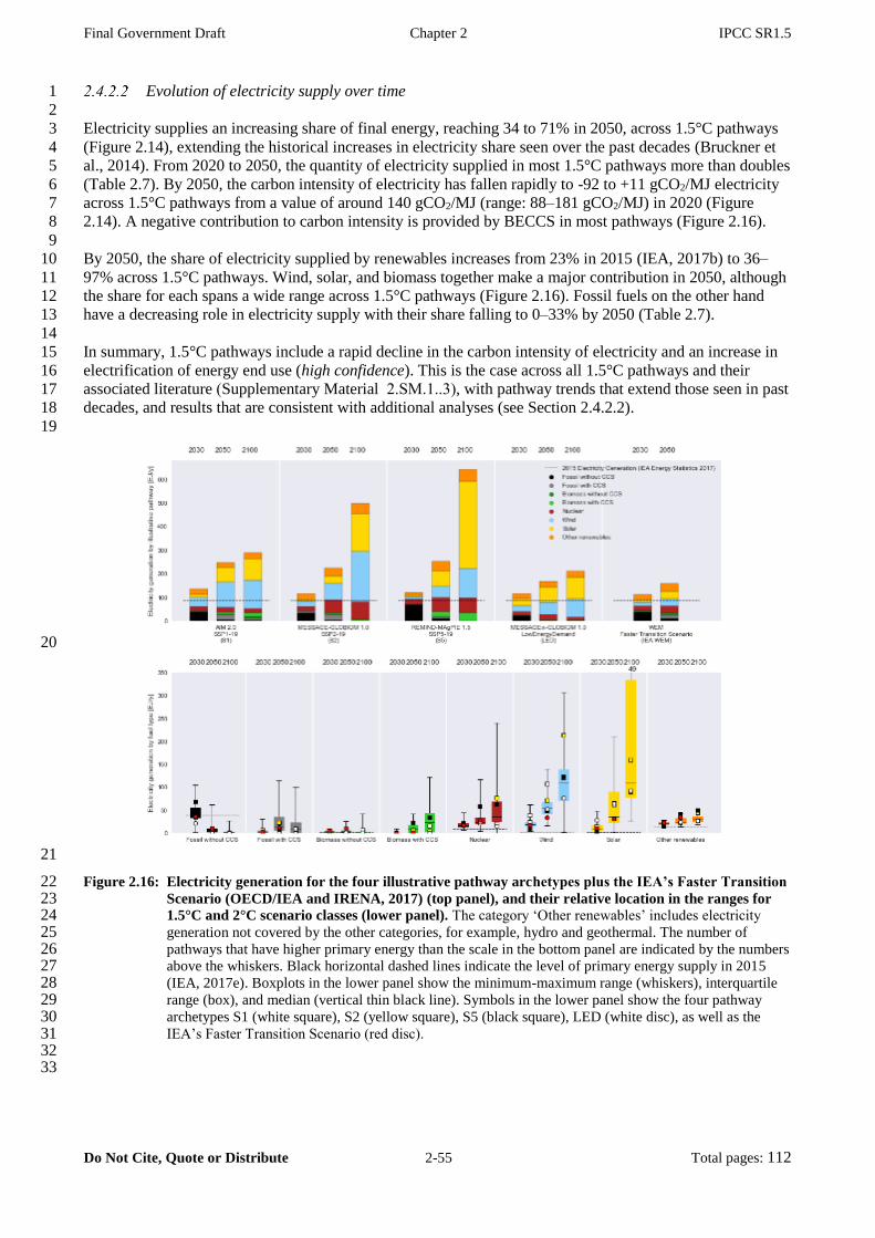
Final Government Draft Chapter 2 IPCC SR1.5
Do Not Cite, Quote or Distribute 2-55 Total pages: 112
Evolution of electricity supply over time 1
2
Electricity supplies an increasing share of final energy, reaching 34 to 71% in 2050, across 1.5°C pathways 3
(Figure 2.14), extending the historical increases in electricity share seen over the past decades (Bruckner et 4
al., 2014). From 2020 to 2050, the quantity of electricity supplied in most 1.5°C pathways more than doubles 5
(Table 2.7). By 2050, the carbon intensity of electricity has fallen rapidly to -92 to +11 gCO2/MJ electricity 6
across 1.5°C pathways from a value of around 140 gCO2/MJ (range: 88–181 gCO2/MJ) in 2020 (Figure 7
2.14). A negative contribution to carbon intensity is provided by BECCS in most pathways (Figure 2.16). 8
9
By 2050, the share of electricity supplied by renewables increases from 23% in 2015 (IEA, 2017b) to 36–10
97% across 1.5°C pathways. Wind, solar, and biomass together make a major contribution in 2050, although 11
the share for each spans a wide range across 1.5°C pathways (Figure 2.16). Fossil fuels on the other hand 12
have a decreasing role in electricity supply with their share falling to 0–33% by 2050 (Table 2.7). 13
14
In summary, 1.5°C pathways include a rapid decline in the carbon intensity of electricity and an increase in 15
electrification of energy end use (high confidence). This is the case across all 1.5°C pathways and their 16
associated literature (Supplementary Material 2.SM.1..3), with pathway trends that extend those seen in past 17
decades, and results that are consistent with additional analyses (see Section 2.4.2.2). 18
19
20
21
Figure 2.16: Electricity generation for the four illustrative pathway archetypes plus the IEA’s Faster Transition 22 Scenario (OECD/IEA and IRENA, 2017) (top panel), and their relative location in the ranges for 23 1.5°C and 2°C scenario classes (lower panel). The category ‘Other renewables’ includes electricity 24 generation not covered by the other categories, for example, hydro and geothermal. The number of 25 pathways that have higher primary energy than the scale in the bottom panel are indicated by the numbers 26 above the whiskers. Black horizontal dashed lines indicate the level of primary energy supply in 2015 27 (IEA, 2017e). Boxplots in the lower panel show the minimum-maximum range (whiskers), interquartile 28 range (box), and median (vertical thin black line). Symbols in the lower panel show the four pathway 29 archetypes S1 (white square), S2 (yellow square), S5 (black square), LED (white disc), as well as the 30 IEA’s Faster Transition Scenario (red disc). 31
32 33
Final Government Draft Chapter 2 IPCC SR1.5
Do Not Cite, Quote or Distribute 2-56 Total pages: 112
Deployment of Carbon Capture and Storage 1
2
Studies have shown the importance of CCS for deep mitigation pathways (Krey et al., 2014a; Kriegler et al., 3
2014b), based on its multiple roles to limit fossil-fuel emissions in electricity generation, liquids production, 4
and industry applications along with the projected ability to remove CO2 from the atmosphere when 5
combined with bioenergy. This remains a valid finding for those 1.5°C and 2°C pathways that do not 6
radically reduce energy demand nor offer carbon-neutral alternatives to liquids and gases that do not rely on 7
bioenergy. 8
9
There is a wide range of CCS that is deployed across 1.5°C pathways (Figure 2.17). A few 1.5°C pathways 10
with very low energy demand do not include CCS at all (Grubler et al., 2018). For example, the LED 11
pathway has no CCS, whereas other pathways like the S5 pathway rely on a large amount of BECCS to get 12
to net-zero carbon emissions. The cumulative fossil and biomass CO2 stored through 2050 ranges from zero 13
to 460 GtCO2 across 1.5°C pathways, with zero up to 190 GtCO2 from biomass captured and stored. Some 14
pathways have very low fossil-fuel use overall, and consequently little CCS applied to fossil fuels. In 1.5°C 15
pathways where the 2050 coal use remains above 20 EJ yr-1 in 2050, 33–100% is combined with CCS. 16
While deployment of CCS for natural gas and coal vary widely across pathways, there is greater natural gas 17
primary energy connected to CCS than coal primary energy connected to CCS in many pathways (Figure 18
2.17). 19
20
CCS combined with fossil-fuel use remains limited in some 1.5°C pathways (Rogelj et al., 2018) as the 21
limited 1.5°C carbon budget penalizes CCS if it is assumed to have incomplete capture rates or if fossil fuels 22
are assumed to continue to have significant lifecycle GHG emissions (Pehl et al., 2017). However, high 23
capture rates are technically achievable now at higher cost, although effort to date have focussed on cost 24
reduction of capture (IEAGHG, 2006; DOE/NETL, 2013). 25
26
The quantity of CO2 stored via CCS over this century in 1.5°C pathways ranges from zero to 1,900 GtCO2, 27
(Figure 2.17). The IPCC Special Report on on Carbon Dioxide Capture and Storage (IPCC, 2005) found that 28
that, worldwide, it is likely that there is a technical potential of at least about 2,000 GtCO2 of storage capacity 29
in geological formations. Furthermore the IPCC (2005) recognised that there could be a much larger 30
potential for geological storage in saline formations, but the upper limit estimates are uncertain due to lack of 31
information and an agreed methodology. Since IPCC (2005), understanding has improved and there have 32
been detailed regional surveys of storage capacity (Vangkilde-Pedersen et al., 2009; Ogawa et al., 2011; Wei 33
et al., 2013; Bentham et al., 2014; Riis and Halland, 2014; Warwick et al., 2014; NETL, 2015) and 34
improvement and standardisation of methodologies (e.g., Bachu et al. 2007a, b). Dooley (2013) synthesised 35
published literature on both the global geological storage resource as well as the potential demand for 36
geologic storage in mitigation pathways, and found that the cumulative demand for CO2 storage was small 37
compared to a practical storage capacity estimate (as defined by Bachu et al., 2007a) of 3,900 GtCO2 38
worldwide. Differences, however, remain in estimates of storage capacity due to, e.g. the potential storage 39
limitations of subsurface pressure build-up (Szulczewski et al., 2014) and assumptions on practices that 40
could manage such issues (Bachu, 2015). Kearns et al. (2017) constructed estimates of global storage 41
capacity of 8,000 to 55,000 GtCO2 (accounting for differences in detailed regional and local estimates), 42
which is sufficient at a global level for this century, but found that at a regional level, robust demand for CO2 43
storage exceeds their lower estimate of regional storage available for some regions. However, storage 44
capacity is not solely determined by the geological setting, and Bachu (2015) describes storage engineering 45
practices that could further extend storage capacity estimates. In summary, the storage capacity of all of 46
these global estimates is larger than the cumulative CO2 stored via CCS of 1.5°C pathways over this century. 47
48
There is uncertainty in the future deployment of CCS given the limited pace of current deployment, the 49
evolution of CCS technology that would be associated with deployment, and the current lack of incentives 50
for large-scale implementation of CCS (Bruckner et al., 2014; Clarke et al., 2014; Riahi et al., 2017). Given 51
the importance of CCS in most mitigation pathways and its current slow pace of improvement, the large-52
scale deployment of CCS as an option depends on the further development of the technology in the near 53
term. Chapter 4 discusses how progress on CCS might be accelerated. 54
55 56

Final Government Draft Chapter 2 IPCC SR1.5
Do Not Cite, Quote or Distribute 2-57 Total pages: 112
1 Figure 2.17: CCS deployment in 1.5°C and 2°C pathways for biomass, coal and natural gas (EJ of primary 2
energy) and the cumulative quantity of fossil (including from, e.g., cement production) and biomass 3 CO2 stored via CCS (lower right in GtCO2 stored). Boxplots show median, interquartile range and full 4 range of pathways in each temperature class. Pathway temperature classes (Table 2.1), illustrative 5 pathway archetypes, and the IEA’s Faster Transition Scenario (IEA WEM) (OECD/IEA and IRENA, 6 2017) are indicated in the legend. 7
8
9
2.4.3 Energy end-use sectors 10
11
Since the power sector is almost decarbonized by mid-century in both 1.5°C and 2°C pathways, major 12
differences come from CO2 emission reductions in end-use sectors. Energy-demand reductions are key and 13
common features in 1.5˚C-consistent pathways, which can be achieved by efficiency improvements and 14
various specific demand-reduction measures. Another important feature is end-use decarbonisation including 15
by electrification, although the potential and challenges in each end-use sector vary significantly. 16
17
In the following sections, the potential and challenges of CO2 emission reductions towards 1.5°C and 2°C- 18
consistent pathways are discussed for each end-use energy sector (industry, buildings, and transport sectors). 19
For this purpose, two types of pathways are analysed and compared: IAM (integrated assessment modelling) 20
studies and sectoral (detailed) studies. IAM data are extracted from the database that was compiled for this 21
assessment (see Supplementary Material 2.SM.1.3), and the sectoral data are taken from a recent series of 22
publications; ‘Energy Technology Perspectives’ (ETP) (IEA, 2014, 2015b, 2016a, 2017a), the IEA/IRENA 23
report (OECD/IEA and IRENA, 2017), and the Shell Sky report (Shell International B.V., 2018). The IAM 24
pathways are categorized according to their temperature rise in 2100 and the overshoot of temperature during 25
the century (see Table 2.1 in Section 2.1). Since the number of Below-1.5°C pathways is small, the 26
following analyses focus only on the featured of the 1.5°C-low-OS and 1.5°C-high-OS pathways (hereafter 27
denoted together as 1.5°C overshoot pathways or IAM-1.5DS-OS) and 2°C-consistent pathways (IAM-2DS). 28
In order to show the diversity of IAM pathways, we again show specific data from the four illustrative 29
pathways archetypes used throughout this chapter (see Sections 2.1 and 2.3). 30
31
IEA ETP-B2DS (‘Beyond 2 Degrees’) and ETP-2DS are pathways with a 50% chance of limiting 32
temperature rise below 1.75°C and 2°C by 2100, respectively (IEA, 2017a). The IEA-66%2DS pathway 33

Final Government Draft Chapter 2 IPCC SR1.5
Do Not Cite, Quote or Distribute 2-58 Total pages: 112
keeps global-mean temperature rise below 2°C not just in 2100 but also over the course of the 21st century 1
with a 66% chance of being below 2°C by 2100 (OECD/IEA and IRENA, 2017). The comparison of CO2 2
emission trajectories between ETP-B2DS and IAM-1.5DS-OS show that these are consistent up to 2060 3
(Figure 2.18). IEA scenarios assume that only a very low level of BECCS is deployed to help offset 4
emissions in difficult-to-decarbonize sectors, and that global energy-related CO2 emissions cannot turn net-5
negative at any time and stay zero from 2060 to 2100 (IEA, 2017a). Therefore, although its temperature rise 6
in 2100 is below 1.75°C rather than below 1.5°C, this scenario can give information related to 1.5°C-7
consistent overshoot pathway up to 2050. The trajectory of IEA-66%2DS (also referred to in other 8
publications as IEA’s ‘Faster Transition Scenario’) lies between IAM-1.5DS-OS and IAM-2DS pathway 9
ranges, and IEA-2DS stays in the range of 2°C-consistent IAM pathways. The Shell-Sky scenario aims to 10
hold the temperature rise to well-below 2°C, but it is a delayed action pathway relative to others, as can be 11
seen in Figure 2.18. 12
13
Energy-demand reduction measures are key to reduce CO2 emissions from end-use sectors for low-carbon 14
pathways. The up-stream energy reductions can be several times to an order of magnitude larger than the 15
initial end-use demand reduction. There are interdependencies among the end-use sectors and also between 16
energy-supply and end-use sectors, which raise the importance of a wide, systematic approach. As shown in 17
Figure 2.19, global final-energy consumption grows by 30% and 10% from 2010 to 2050 for 2°C-consistent 18
and 1.5°C overshoot pathways from IAMs, respectively, while much higher growth of 75% is projected for 19
reference scenarios. The ranges within a specific pathway class are due to a variety of factors as introduced 20
in Section 2.3.1, as well as differences between modelling frameworks. The important energy efficiency 21
improvements and energy conservation that facilitate many of the 1.5°C pathways raise the issue of potential 22
rebound effects (Saunders, 2015), which, while promoting development, can make the achievement of low-23
energy demand futures more difficult than modelling studies anticipate (see Sections 2.5 and 2.6). 24
25
26 Figure 2.18: Comparison of CO2 emission trajectories of sectoral pathways (IEA ETP-B2DS, ETP-2DS, IEA-27
66%2DS, Shell-Sky) with the ranges of IAM pathway (2DS are 2°C-consistent pathways and 1.5DS-OS 28 are1.5°C-consistent overshoot pathways). The CO2 emissions shown here are the energy-related 29 emissions including industrial process emissions. 30
31

Final Government Draft Chapter 2 IPCC SR1.5
Do Not Cite, Quote or Distribute 2-59 Total pages: 112
1 Figure 2.19: (a) Global final energy, (b) direct CO2 emissions from the all energy demand sectors, (c) carbon 2
intensity, and (d) structure of final energy (electricity, liquid fuel, coal, and biomass). The squares 3 and circles indicate the IAM archetype pathways and diamonds the data of sectoral scenarios. The red 4 dotted line indicates the 2010 level. H2DS: Higher-2°C, L2DS: Lower-2°C, 1.5DS-H: 1.5°C-high-OS, 5 1.5DS-L: 1.5°C-low-OS, 1.5DS = 1.5DS-OS: 1.5°C-consistent pathways with overshoot. Section 2.1 for 6 descriptions. 7
8
Final-energy demand is driven by demand in energy services for mobility, residential and commercial 9
activities (buildings), and manufacturing. This heavily depends on assumptions about socio-economic 10
futures as represented by the SSPs (Bauer et al., 2017) (see Sections 2.1, 2.3 and 2.5). The structure of this 11
demand drives the composition of final energy use in terms of energy carriers (electricity, liquids, gases, 12
solids, hydrogen etc.). 13
14
Figure 2.19 shows the structure of global final energy demand in 2030 and 2050, indicating the trend toward 15
electrification and fossil fuel usage reduction. This trend is more significant in 1.5°C pathways than 2°C 16
pathways. Electrification continues throughout the second half of the century leading to a 3.5 to 6-fold 17
increase in electricity demand (interquartile range; median 4.5) by the end of the century relative to today 18
(Grubler et al., 2018; Luderer et al., 2018). Since the electricity sector is completely decarbonised by mid-19
century in 1.5°C pathways (see Figure 2.20), electrification is the primary means to decarbonize energy end-20
use sectors. 21
22
The CO2 emissions6 of end-use sectors and carbon intensity are shown in Figure 2.20. The projections of 23
IAMs and IEA studies show rather different trends, especially in the carbon intensity. These differences 24
come from various factors, including the deployment of CCS, the level of fuel switching and efficiency 25
6: This section reports “direct” CO2 emissions as reported for pathways in the database for the report. As shown below, the emissions
from electricity are nearly zero around 2050, so the impact of indirect emissions on the whole emission contributions of each sector
is very small in 2050.

Final Government Draft Chapter 2 IPCC SR1.5
Do Not Cite, Quote or Distribute 2-60 Total pages: 112
improvements, and the effect of structural and behavioural changes. IAM projections are generally optimistic 1
for the industry sectors, but not for buildings and transport sectors. Although GDP increases by a factor of 2
3.4 from 2010 to 2050, the total energy consumption of end-use sectors grows by only about 30% and 20% 3
in 1.5°C overshoot and 2°C-consistent pathways, respectively. However, CO2 emissions would need to be 4
reduced further to achieve the stringent temperature limits. Fig. 2.20 shows that the reduction in CO2 5
emissions of end-use sectors is larger and more rapid in 1.5°C overshoot than 2°C-consistent pathways, 6
while emissions from the power sector are already almost zero in 2050 in both sets of pathways indicating 7
that supply-side emissions reductions are almost fully exploited already in 2°C-consistent pathways (see 8
Figure 2.20) (Rogelj et al., 2015b, 2018; Luderer et al., 2016b). The emission reductions in end-use sectors is 9
largely made possible due to efficiency improvements, demand reduction measures and electrification, but 10
its level differs among end-use sectors. While the carbon intensity of industry and the buildings sector 11
decreases to a very low level of around 10 gCO2 MJ-1, the carbon intensity of transport becomes the highest 12
of any sector by 2040 due to its higher reliance on oil-based fuels. In the following subsections, the potential 13
and challenges of CO2 emission reduction in each end-use sector are discussed in detail. 14
15
16 Figure 2.20: Comparison of (a) direct CO2 emissions and (b) carbon intensity of the power and energy end-use 17
sectors (industry, buildings, and transport sectors) between IAMs and sectoral studies (IEA-ETP 18 and IEA/IRENA). Diamond markers in panel (b) show data for IEA-ETP scenarios (2DS and B2DS), 19 and IEA/IRENA scenario (66%2DS). Note: for the data of IAM studies, there is rather large variation of 20 projections for each indicator. Please see the details in the following figures in each end-use sector 21 section. 22
23
24
Industry 25
26
The industry sector is the largest end-use sector both in terms of final-energy demand and GHG emissions. 27
Its direct CO2 emissions currently account for about 25% of total energy-related and process CO2 emissions, 28
and have increased with an average annual rate of 3.4% between 2000 and 2014, significantly faster than 29
total CO2 emissions (Hoesly et al., 2018). In addition to emissions from the combustion of fossil fuels, non-30
energy uses of fossil fuels in the petro-chemical industry and metal smelting, as well as non-fossil fuel 31
process emissions (e.g., from cement production) contribute a small amount (~5%) to the sector’s CO2 32
emissions inventory. Material industries are particularly energy and emissions intensive: steel, non-ferrous 33
metals, chemicals, non-metallic minerals, and pulp and paper alone accounted for close to 66% of final-34
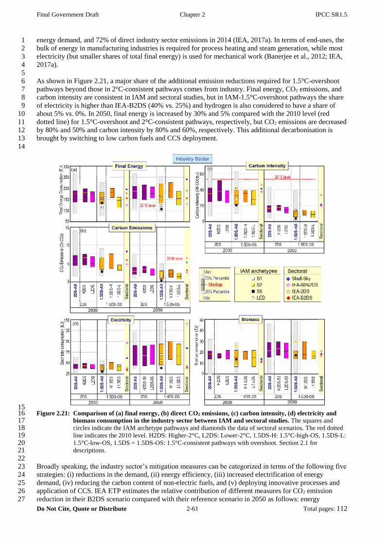
Final Government Draft Chapter 2 IPCC SR1.5
Do Not Cite, Quote or Distribute 2-61 Total pages: 112
energy demand, and 72% of direct industry sector emissions in 2014 (IEA, 2017a). In terms of end-uses, the 1
bulk of energy in manufacturing industries is required for process heating and steam generation, while most 2
electricity (but smaller shares of total final energy) is used for mechanical work (Banerjee et al., 2012; IEA, 3
2017a). 4
5
As shown in Figure 2.21, a major share of the additional emission reductions required for 1.5°C-overshoot 6
pathways beyond those in 2°C-consistent pathways comes from industry. Final energy, CO2 emissions, and 7
carbon intensity are consistent in IAM and sectoral studies, but in IAM-1.5°C-overshoot pathways the share 8
of electricity is higher than IEA-B2DS (40% vs. 25%) and hydrogen is also considered to have a share of 9
about 5% vs. 0%. In 2050, final energy is increased by 30% and 5% compared with the 2010 level (red 10
dotted line) for 1.5°C-overshoot and 2°C-consistent pathways, respectively, but CO2 emissions are decreased 11
by 80% and 50% and carbon intensity by 80% and 60%, respectively. This additional decarbonisation is 12
brought by switching to low carbon fuels and CCS deployment. 13
14
15 Figure 2.21: Comparison of (a) final energy, (b) direct CO2 emissions, (c) carbon intensity, (d) electricity and 16
biomass consumption in the industry sector between IAM and sectoral studies. The squares and 17 circles indicate the IAM archetype pathways and diamonds the data of sectoral scenarios. The red dotted 18 line indicates the 2010 level. H2DS: Higher-2°C, L2DS: Lower-2°C, 1.5DS-H: 1.5°C-high-OS, 1.5DS-L: 19 1.5°C-low-OS, 1.5DS = 1.5DS-OS: 1.5°C-consistent pathways with overshoot. Section 2.1 for 20 descriptions. 21
22
Broadly speaking, the industry sector’s mitigation measures can be categorized in terms of the following five 23
strategies: (i) reductions in the demand, (ii) energy efficiency, (iii) increased electrification of energy 24
demand, (iv) reducing the carbon content of non-electric fuels, and (v) deploying innovative processes and 25
application of CCS. IEA ETP estimates the relative contribution of different measures for CO2 emission 26
reduction in their B2DS scenario compared with their reference scenario in 2050 as follows: energy 27
Final Government Draft Chapter 2 IPCC SR1.5
Do Not Cite, Quote or Distribute 2-62 Total pages: 112
efficiency 42%, innovative process and CCS 37%, switching to low carbon fuels and feed-stocks 13% and 1
material efficiency (include efficient production and use to contribute to demand reduction) 8%. The 2
remainder of this section delves more deeply into the potential mitigation contributions of these strategies as 3
well as their limitations. 4
5
Reduction in the use of industrial materials, while delivering similar services, or improving the quality of 6
products could help to reduce energy demand and overall system-level CO2 emissions. Strategies include 7
using materials more intensively, extension of product lifetimes, increasing recycling, and increasing inter-8
industry material synergies, such as clinker substitution in cement production (Allwood et al., 2013; IEA, 9
2017a). Related to material efficiency, use of fossil-fuel feed-stocks could shift to lower-carbon feed-stocks 10
such as oil to natural gas and biomass and end-uses could shift to more sustainable materials such as 11
biomass-based materials, reducing the demand for energy-intensive materials (IEA, 2017a). 12
13
Reaping energy efficiency potentials hinges critically on advanced management practices in industrial 14
facilities such as energy management systems, as well as targeted policies to accelerate adoption of best 15
available technology (see Section 2.5). Although excess energy, usually as waste heat, is inevitable, 16
recovering and reusing this waste heat under economically and technically viable conditions benefits the 17
overall energy system. Furthermore, demand-side management strategies could modulate the level of 18
industrial activity in line with the availability of resources in the power system. This could imply a shift 19
away from peak demand and as power supply decarbonizes, this demand-shaping potential could shift some 20
load to times with high portions of low-carbon electricity generation (IEA, 2017a). 21
22
In the industry sector, energy demand increases more than 40% between 2010 and 2050 in baseline 23
scenarios. However, in the 1.5°C-overshoot and 2°C-consistent pathways from IAMs, the increase is only 24
30% and 5%, respectively (Figure 2.21). These energy demand reductions encompass both efficiency 25
improvements in production as well as reductions in material demand, as most IAMs do not discern these 26
two factors. 27
28
CO2 emissions from industry increase by 30% in 2050 compared to 2010 in baseline scenarios. By contrast, 29
these emissions are reduced by 80% and 50% relative to 2010 levels in 1.5°C-overshoot and 2°C-consistent 30
pathways from IAMs, respectively (Figure 2.21). By mid-century, CO2 emissions per unit electricity are 31
projected to decrease to near zero in both sets of pathways (see Figure 2.20). An accelerated electrification of 32
the industry sector thus becomes an increasingly powerful mitigation option. In the IAM pathways, the share 33
of electricity increases up to 30% by 2050 in 1.5°C-overshoot pathways (Figure 2.21) from 20% in 2010. 34
Some industrial fuel uses are substantially more difficult to electrify than others, and electrification would 35
have other effects on the process, including impacts on plant design, cost and available process integration 36
options (IEA, 2017a)7. 37
38
In 1.5°C-overshoot pathways, the carbon intensity of non-electric fuels consumed by industry decreases to 39
16 gCO2 MJ-1 by 2050, compared to 25 gCO2 MJ-1 in 2°C-consistent pathways. Considerable carbon 40
intensity reductions are already achieved by 2030, largely via a rapid phase-out of coal. Biomass becomes an 41
increasingly important energy carrier in the industry sector in deep-decarbonisation pathways, but primarily 42
in the longer term (in 2050, biomass accounts for only 10% of final energy consumption even in 1.5°C-43
overshoot pathways). In addition, hydrogen plays a considerable role as a substitute for fossil-based non-44
electric energy demands in some pathways. 45
46
Without major deployment of new sustainability-oriented low-carbon industrial processes, the 1.5°C-47
overshoot target is difficult to achieve. Bringing such technologies and processes to commercial deployment 48
requires significant investment in research and development. Some examples of innovative low-carbon 49
process routes include: new steelmaking processes such as upgraded smelt reduction and upgraded direct 50
reduced iron, inert anodes for aluminium smelting, and full oxy-fuelling kilns for clinker production in 51
cement manufacturing (IEA, 2017a). 52
7: Electrification can be linked with the heating and drying process by electric boilers and electro-thermal processes, and also low-
temperature heat demand by heat pumps. In iron and steel industry, hydrogen produced by electrolysis can be used as a reduction
agent of iron instead of coke. Excess resources, such as black liquor will provide the opportunity to increase the systematic efficiency
to use for electricity generation.

Final Government Draft Chapter 2 IPCC SR1.5
Do Not Cite, Quote or Distribute 2-63 Total pages: 112
1
CCS plays a major role in decarbonizing the industry sector in the context of 1.5°C and 2°C pathways, 2
especially in industries with higher process emissions, such as cement, iron and steel industries. In 1.5°C-3
overshoot pathways, CCS in industry reaches 3 GtCO2 yr-1 by 2050, albeit with strong variations across 4
pathways. Given project long-lead times and the need for technological innovation, early scale-up of industry 5
CCS is essential to achieve the stringent temperature target. Development and demonstration of such projects 6
has been slow, however. Currently, only two large-scale industrial CCS projects outside of oil and gas 7
processing are in operation (Global CCS Institute, 2016). The estimated current cost8 of CO2 avoided (in 8
2015-US$) ranges from $20-27 tCO2-1 for gas processing and bio-ethanol production, and $60-138 tCO2
-1 for 9
fossil fuel-fired power generation up to $104-188 tCO2-1 for cement production (Irlam, 2017). 10
11
12
Buildings 13
14
In 2014, the buildings sector accounted for 31% of total global final-energy use, 54% of final-electricity 15
demand, and 8% of energy-related CO2 emissions (excluding indirect emission due to electricity). When 16
upstream electricity generation is taken into account, buildings were responsible for 23% of global energy-17
related CO2 emissions, with one-third of those from direct fossil fuel consumption (IEA, 2017a). 18
19
Past growth of energy consumption has been mainly driven by population and economic growth, with 20
improved access to electricity, and higher use of electrical appliances and space cooling resulting from 21
increasing living standards, especially in developing countries (Lucon et al., 2014). These trends will 22
continue in the future and in 2050, energy consumption is projected to increase by 20% (50%) compared to 23
2010 in IAM-1.5°C-overshoot (2°C-consistent) pathways (Figure 2.22). However, sectoral studies (IEA-ETP 24
scenarios) show different trends. Energy consumption in 2050 decreases compared to 2010 in ETP-B2DS, 25
and the reduction rate of CO2 emissions is higher than in IAM pathways (Figure 2.22). Mitigation options 26
are often more widely covered in sectoral studies (Lucon et al., 2014), leading to greater reductions in energy 27
consumption and CO2 emissions. 28
29
Emissions reductions are driven by a clear tempering of energy demand and a strong electrification of the 30
buildings sector. The share of electricity in 2050 is 60% in 1.5°C-overshoot pathways, compared with 50% 31
in 2°C-consistent pathways (Figure 2.22). Electrification contributes to the reduction of direct CO2 emissions 32
by replacing carbon-intensive fuels, like oil and coal. Furthermore, when combined with a rapid 33
decarbonisation of the power system (see Section 2.4.1) it also enables further reduction of indirect CO2 34
emissions from electricity. Sectoral bottom-up models in general estimate lower electrification potentials for 35
the buildings sector in comparison to global IAMs (see Figure 2.22). Besides CO2 emissions, increasing 36
global demand for air conditioning in buildings may also lead to increased emissions of HFCs in this sector 37
over the next few decades. Although these gases are currently a relatively small proportion of annual GHG 38
emissions, their use in the air conditioning sector is expected to grow rapidly over the next few decades if 39
alternatives are not adopted. However, their projected future impact can be significantly mitigated through 40
better servicing and maintenance of equipment and switching of cooling gases (Shah et al., 2015; Purohit and 41
Höglund-Isaksson, 2017). 42
43
IEA-ETP (IEA, 2017a) analysed the relative importance of various technology measures toward the 44
reduction of energy and CO2 emissions in the buildings sector. The largest energy savings potential is in 45
heating and cooling demand largely due to building envelope improvements and high efficiency and 46
renewable equipment. In the ETP-B2DS, energy demand for space heating and cooling is 33% lower in 2050 47
than the reference scenario and these reductions account for 54% of total reductions from the reference 48
scenario. Energy savings from shifts to high-performance lighting, appliances, and water heating equipment 49
account for a further 24% of the total reduction. The long-term, strategic shift away from fossil-fuel use in 50
buildings, alongside the rapid uptake of energy efficient, integrated and renewable energy technologies (with 51
clean power generation), leads to a drastic reduction of CO2 emissions. In ETP-B2DS, the direct CO2 52
emissions are 79% lower than the reference scenario in 2050 and the remaining emissions come mainly from 53
the continued use of natural gas. 54
55
8: These are first-of-a-kind (FOAK) cost data.

Final Government Draft Chapter 2 IPCC SR1.5
Do Not Cite, Quote or Distribute 2-64 Total pages: 112
The buildings sector is characterized by very long-living infrastructure and immediate steps are hence 1
important to avoid lock-in of inefficient carbon and energy-intensive buildings. This applies both to new 2
buildings in developing countries where substantial new construction is expected in the near future and to 3
retrofits of existing building stock in developed regions. This represents both a significant risk and 4
opportunity for mitigation9. A recent study highlights the benefits of deploying the most advanced 5
renovation technologies, which would avoid lock-in into less efficient measures (Güneralp et al., 2017). 6
Aside from the effect of building envelope measures, adoption of energy-efficient technologies such as heat 7
pumps and more recently light-emitting diodes is also important for the reduction of energy and CO2 8
emissions (IEA, 2017a). Consumer choices, behaviour and building operation can also significantly affect 9
energy consumption (see Section 4.3). 10
11
12 Figure 2.22: Comparison of (a) final energy, (b) direct CO2 emissions, (c) carbon intensity, (d) electricity and 13
biomass consumption in the buildings sector between IAM and sectoral studies. The squares and 14 circles indicate the IAM archetype pathways and diamonds the data of sectoral scenarios. The red dotted 15 line indicates the 2010 level. H2DS: Higher-2°C, L2DS: Lower-2°C, 1.5DS-H: 1.5°C-high-OS, 1.5DS-L: 16 1.5°C-low-OS, 1.5DS = 1.5DS-OS: 1.5°C-consistent pathways with overshoot. Section 2.1 for 17 descriptions. 18
19
20
21
9: In this section, we only discuss the direct emissions from the sector, but the selection of building materials have a significant
impact on the reduction of energy and emissions during the production, such as shift from the steel and concrete to wood-based
materials.
Final Government Draft Chapter 2 IPCC SR1.5
Do Not Cite, Quote or Distribute 2-65 Total pages: 112
Transport 1
2
Transport accounted for 28% of global final-energy demand and 23% of global energy-related CO2 3
emissions in 2014. Emissions increased by 2.5% annually between 2010 and 2015, and over the past half 4
century the sector has witnessed faster emissions growth than any other. The transport sector is the least 5
diversified energy end-use sector; the sector consumed 65% of global oil final-energy demand, with 92% of 6
transport final-energy demand consisting of oil products (IEA, 2017a), suggesting major challenges for deep 7
decarbonisation. 8
9
Final energy, CO2 emissions, and carbon intensity for the transport sector are shown in Figure 2.23. The 10
projections of IAMs are more pessimistic than IEA-ETP scenarios, though both clearly project deep cuts in 11
energy consumption and CO2 emissions by 2050. For example, 1.5°C-overshoot pathways from IAMs 12
project a reduction of 15% in energy consumption between 2015 and 2050, while ETP-B2DS projects a 13
reduction of 30% (Figure 2.23). Furthermore, IAM pathways are generally more pessimistic in the 14
projections of CO2 emissions and carbon intensity reductions. In AR5 (Clarke et al., 2014; Sims et al., 2014), 15
similar comparisons between IAMs and sectoral studies were performed and these were in good agreement 16
with each other. Since the AR5, two important changes can be identified; rapid growth of electric vehicle 17
sales in passenger cars, and more attention towards structural changes in this sector. The former contributes 18
to reduction of CO2 emissions and the latter reduction of energy consumption. 19
20
Deep emissions reductions in the transport sector would be achieved by several means. Technology focused 21
measures such as energy efficiency and fuel-switching are two of these. Structural changes that avoid or shift 22
transport activity are also important. While the former solutions (technologies) always tend to figure into 23
deep decarbonisation pathways in a major way, this is not always the case with the latter, especially in IAM 24
pathways. Comparing different types of global transport models, Yeh et al. (2016) find that sectoral 25
(intensive) studies generally envision greater mitigation potential from structural changes in transport 26
activity and modal choice. Though, even there, it is primarily the switching of passengers and freight from 27
less- to more-efficient travel modes (e.g., cars, trucks and airplanes to buses and trains) that is the main 28
strategy; other actions, such as increasing vehicle load factors (occupancy rates) and outright reductions in 29
travel demand (e.g., as a result of integrated transport, land-use and urban planning), figure much less 30
prominently. Whether these dynamics accurately reflect the actual mitigation potential of structural changes 31
in transport activity and modal choice is a point of investigation. According to the recent IEA-ETP scenarios, 32
the share of avoid (reduction of mobility demand) and shift (shifting to more efficient modes) measures in 33
the reduction of CO2 emissions from the reference to B2DS scenarios in 2050 amounts to 20% (IEA, 2017a). 34
35
The potential and strategies to reduce energy consumption and CO2 emissions differ significantly among 36
transport modes. In ETP-B2DS, the shares of energy consumption and CO2 emissions in 2050 for each mode 37
are rather different (see Table 2.8), indicating the challenge of decarbonizing heavy-duty vehicles (HDV, 38
trucks), aviation, and shipping. The reduction of CO2 emissions in the whole sector from the reference 39
scenario to ETP-B2DS is 60% in 2050, with varying contributions per mode (Table 2.8). Since there is no 40
silver bullet for this deep decarbonisation, every possible measure would be required to achieve this stringent 41
emissions outcome. The contribution of various measures for the CO2 emission reduction from the reference 42
scenario to the IEA-B2DS in 2050 can be decomposed to efficiency improvement (29%), biofuels (36%), 43
electrification (15%), and avoid/shift (20%) (IEA, 2017a). It is noted that the share of electrification becomes 44
larger compared with older studies, reflected by the recent growth of electric vehicle sales worldwide. 45
Another new trend is the allocation of biofuels to each mode of transport. In IEA-B2DS, the total amount of 46
biofuels consumed in the transport sector is 24EJ10 in 2060, and allocated to LDV (light-duty vehicles, 17%), 47
HDV (35%), aviation (28%), and shipping (21%), that is, more biofuels is allocated to the difficult-to-48
decarbonize modes (see Table 2.8). 49
50
51
10: This is estimated for the biofuels produced in a "sustainable manner" from non-food crop feed-stocks, which are capable of
delivering significant lifecycle GHG emissions savings compared with fossil fuel alternatives, and which do not directly compete
with food and feed crops for agricultural land or cause adverse sustainability impacts.

Final Government Draft Chapter 2 IPCC SR1.5
Do Not Cite, Quote or Distribute 2-66 Total pages: 112
Table 2.8: Transport sector indicators by mode in 2050 (IEA, 2017a). Share of Energy consumption, biofuel 1 consumption, CO2 emissions, and reduction of energy consumption and CO2 emissions from 2014. (CO2 2 emissions are Well-to-Wheel emissions, including the emission during the fuel production.), LDV: Light 3 Duty Vehicle, HDV: Heavy Duty Vehicle 4
5 Share of each mode (%) Reduction from 2014 (%)
Energy Biofuel CO2 Energy CO2
LDV 36 17 30 51 81
HDV 33 35 36 8 56
Rail 6 -1 -136 107
Aviation 12 28 14 14 56
Shipping 17 21 21 26 29
6
In road transport, incremental vehicle improvements (including engines) are relevant, especially in the short 7
to medium term. Hybrid electric vehicles (HEVs) are also instrumental to enabling the transition from ICEs 8
(internal combustion engine vehicles) to electric vehicles, especially plug-in hybrid electric vehicles 9
(PHEVs). Electrification is a powerful measure to decarbonize short-distance vehicles (passenger cars and 10
two and three wheelers) and the rail sector. In road freight transport (trucks), systemic improvements (e.g., in 11
supply chains, logistics, and routing) would be effective measures with efficiency improvement of vehicles. 12
Shipping and aviation are more challenging to decarbonize, while their demand growth is projected to be 13
higher than other transport modes. Both modes would need to pursue highly ambitious efficiency 14
improvements and use of low-carbon fuels. In the near and medium term, this would be advanced biofuels 15
while in the long term it could be hydrogen as direct use for shipping or an intermediate product for synthetic 16
fuels for both modes (IEA, 2017a). 17
18
The share of low-carbon fuels in the total transport fuel mix increases to 10% (16%) by 2030 and to 40% 19
(58%) by 2050 in 1.5°C-overshoot pathways from IAMs. The IEA-B2DS scenario is on the more ambitious 20
side, especially in the share of electricity. Hence, there is wide variation among scenarios, including the IAM 21
pathways, regarding changes in the transport fuel mix over the first half of the century. As seen in Figure 22
2.23, the projections of energy consumption, CO2 emissions, and carbon intensity are quite different between 23
IAM and ETP scenarios. These differences can be explained by more weight on efficiency improvements 24
and avoid/shift decreasing energy consumption, and the higher share of biofuels and electricity accelerating 25
the speed of decarbonisation in ETP scenarios. Although biofuel consumption and electric vehicle sales have 26
increased significantly in recent years, the growth rates projected in these pathways would be unprecedented 27
and far higher than has been experienced to date. 28
29

Final Government Draft Chapter 2 IPCC SR1.5
Do Not Cite, Quote or Distribute 2-67 Total pages: 112
1 Figure 2.23: Comparison of (a) final energy, (b) direct CO2 emissions, (c) carbon intensity, (d) electricity and 2
biofuel consumption in the transport sector between IAM and sectoral studies. The squares and 3 circles indicate the IAM archetype pathways and diamonds the data of sectoral scenarios. The red dotted 4 line indicates the 2010 level. H2DS: Higher-2°C, L2DS: Lower-2°C, 1.5DS-H: 1.5°C-high-OS, 1.5DS-L: 5 1.5°C-low-OS, 1.5DS = 1.5DS-OS: 1.5°C-consistent pathways with overshoot. Section 2.1 for 6 descriptions. 7
8
1.5°C pathways require an acceleration of the mitigation solutions already featured in 2°C-consistent 9
pathways (e.g., more efficient vehicle technologies operating on lower-carbon fuels), as well as those having 10
received lesser attention in most global transport decarbonisation pathways up to now (e.g., mode-shifting 11
and travel demand management). Current-generation, global pathways generally do not include these newer 12
transport sector developments, whereby technological solutions are related to shifts in traveller’s behaviour. 13
14
15
2.4.4 Land-use transitions and changes in the agricultural sector 16
17
The agricultural and land system described together under the umbrella of the AFOLU (Agriculture, 18
Forestry, and Other Land Use) sector plays an important role in 1.5°C pathways (Clarke et al., 2014; Smith 19
and Bustamante, 2014; Popp et al., 2017). On the one hand, its emissions need to be limited over the course 20
of this century to be in line with pathways limiting warming to 1.5°C (see Sections 2.2-3). On the other hand, 21
the AFOLU system is responsible for food and feed production, for wood production for pulp and 22
construction, for the production of biomass that is used for energy, CDR or other uses, and for the supply of 23
non-provisioning (ecosystem) services (Smith and Bustamante, 2014). Meeting all demands together 24
requires changes in land use, as well as in agricultural and forestry practices, for which a multitude of 25
Final Government Draft Chapter 2 IPCC SR1.5
Do Not Cite, Quote or Distribute 2-68 Total pages: 112
potential options have been identified (Smith and Bustamante, 2014; Popp et al., 2017) (see also 1
Supplementary Material 2.SM.1.2 and Chapter 4, Section 4.3.1, 4.3.2 and 4.3.7). 2
3
This section assesses the transformation of the AFOLU system, mainly making use of pathways from IAMs 4
(see Section 2.1) that are based on quantifications of the SSPs and that report distinct land-use evolutions in 5
line with limiting warming to 1.5°C (Calvin et al., 2017; Fricko et al., 2017; Fujimori, 2017; Kriegler et al., 6
2017; Popp et al., 2017; Riahi et al., 2017; van Vuuren et al., 2017b; Doelman et al., 2018; Rogelj et al., 7
2018). The SSPs were designed to vary mitigation challenges (O’Neill et al., 2014) (Cross-Chapter Box 1.1), 8
including for the AFOLU sector (Popp et al., 2017; Riahi et al., 2017). The SSP pathway ensemble hence 9
allows for a structured exploration of AFOLU transitions in the context of climate change mitigation in line 10
with 1.5°C, taking into account technological and socio-economic aspects. Other considerations, like food 11
security, livelihoods and biodiversity, are also of importance when identifying AFOLU strategies. These are 12
at present only tangentially explored by the SSPs. Further assessments of AFOLU mitigation options are 13
provided in other parts of this report and in the IPCC AR6 Special Report on Climate Change and Land 14
(SRCCL). Chapter 4 provides an assessment of bioenergy (including feedstocks, see Section 4.3.1), livestock 15
management (Section 4.3.1), reducing rates of deforestation and other land-based mitigation options (as 16
mitigation and adaptation option, see Section 4.3.2), and BECCS, Afforestation and Reforestation options 17
(including the bottom-up literature of their sustainable potential, mitigation cost and side effects, Section 18
4.3.7). Chapter 3 discusses impacts land-based CDR (Cross-Chapter Box 7 in Chapter 3). Chapter 5 assesses 19
the sustainable development implications of AFOLU mitigation, including impacts on biodiversity (Section 20
5.4). Finally, the SRCCL will undertake a more comprehensive assessment of land and climate change 21
aspects. For the sake of complementarity, this section focusses on the magnitude and pace of land transitions 22
in 1.5°C pathways, as well as on the implications of different AFOLU mitigation strategies for different land 23
types. The interactions with other societal objectives and potential limitations of identified AFOLU measures 24
link to these large-scale evolutions, but these are assessed elsewhere (see above). 25
26
Land-use changes until mid-century occur in the large majority of SSP pathways, both under stringent and in 27
absence of mitigation (Figure 2.24). In the latter case, changes are mainly due to socio-economic drivers like 28
growing demands for food, feed and wood products. General transition trends can be identified for many 29
land types in 1.5°C pathways, which differ from those in baseline scenarios and depend on the interplay with 30
mitigation in other sectors (Figure 2.24) (Popp et al., 2017; Riahi et al., 2017; Rogelj et al., 2018). Mitigation 31
that demands land mainly occurs at the expense of agricultural land for food and feed production. 32
Additionally, some biomass is projected to be grown on marginal land or supplied from residues and waste, 33
but at lower shares. Land for second generation energy crops (such as miscanthus or poplar) expands by 34
2030 and 2050 in all available pathways that assume a cost-effective achievement of a 1.5°C temperature 35
goal in 2100 (Figure 2.24), but the scale depends strongly on underlying socioeconomic assumptions (see 36
later discussion of land pathway archetypes). Reducing rates of deforestation restricts agricultural expansion 37
and forest cover can expand strongly in 1.5°C and 2°C pathways alike compared to its extent in no-climate 38
policy baselines due to reduced deforestation, afforestation and reforestation measures. However, the extent 39
to which forest cover expands varies highly across models in the literature, with some models projecting 40
forest cover to stay virtually constant or decline slightly. This is due to whether afforestation and 41
reforestation is included as a mitigation technology in these pathways and interactions with other sectors. 42
43
As a consequence of other land use changes, pasture land is generally projected to be reduced compared to 44
both baselines in which no climate change mitigation action is undertaken and 2°C-consistent pathways. 45
Furthermore, cropland for food and feed production decreases in most 1.5°C pathways, both compared to a 46
no-climate baseline and relative to 2010. These reductions in agricultural land for food and feed production 47
are facilitated by intensification on agricultural land and in livestock production systems (Popp et al., 2017), 48
as well as changes in consumption patterns (Frank et al., 2017; Fujimori, 2017) (see also 4.3.2 for an 49
assessment of these mitigation options). For example, in a scenario based on rapid technological progress 50
(Kriegler et al., 2017), global average cereal crop yields in 2100 are assumed to be above 5 tDM/ha.yr in 51
mitigation scenarios aiming at limiting end-of-century radiative forcing to 4.5 or 2.6 W/m2, compared to 4 52
tDM/ha.yr in the SSP5 baseline to ensure the same food production. Similar improvements are present in 53
1.5°C variants of such scenarios. Historically, cereal crop yields are estimated at 1 tDM/ha.yr and ca. 3 54
tDM/ha.yr in 1965 and 2010, respectively (calculations based on FAOSTAT, 2017). For aggregate energy 55
crops, models assume 4.2-8.9 tDM/ha.yr in 2010, increasing to about 6.9-17.4 tDM/ha.yr in 2050, which fall 56
within the range found in the bottom-up literature yet depend on crop, climatic zone, land quality, and plot 57

Final Government Draft Chapter 2 IPCC SR1.5
Do Not Cite, Quote or Distribute 2-69 Total pages: 112
size (Searle and Malins, 2014). 1
2
3 Figure 2.24: Overview of land-use change transitions in 2030 and 2050, relative to 2010 based on pathways 4
based on the Shared Socioeconomic Pathways (SSP) (Popp et al., 2017; Riahi et al., 2017; Rogelj et 5 al., 2018). Grey: no-climate-policy baseline; green: 2.6 W/m2 pathways; blue: 1.9 W/m2 pathways. Pink: 6 1.9 W/m2 pathways grouped per underlying socioeconomic assumption (from left to right: SSP1 7 sustainability, SSP2 middle-of-the-road, SSP5 fossil-fuelled development). Ranges show the minimum-8 maximum range across the SSPs. Single pathways are shown with plus signs. Illustrative archetype 9 pathways are highlighted with distinct icons. Each panel shows the changes for a different land type. 1.9 10 and 2.6 W/m2 are taken as proxies for 1.5°C and 2°C pathways, respectively. 2.6 W/m2 pathways are 11 mostly consistent with the Lower-2°C and Higher-2°C pathway classes. 1.9 W/m2 pathways are 12 consistent with the 1.5°C-low-OS (mostly SSP1 and SSP2) and 1.5°C-high-OS (SSP5) pathway classes. 13 In 2010, pasture was estimated to cover about 3-3.5 103 Mha, food and feed crops about 1.5-1.6 103 Mha, 14 energy crops about 0-14 Mha and forest about 3.7-4.2 103 Mha, across the models that reported SSP 15 pathways (Popp et al., 2017). 16
17
The pace of projected land transitions over the coming decades can differ strongly between 1.5°C and 18
baseline scenarios without climate change mitigation and from historical trends (Table 2.9). However, there 19
is uncertainty in the sign and magnitude of these future land-use changes (Prestele et al., 2016; Popp et al., 20
2017; Doelman et al., 2018). The pace of projected cropland changes overlaps with historical trends over the 21
past four decades, but in several cases also goes well beyond this range. By the 2030-2050 period, the 22
projected reductions in pasture and potentially strong increases in forest cover imply a reversed dynamic 23
compared to historical and baseline trends. For forest increases, this suggests that distinct policy and 24
government measures would be needed to achieve this, particularly in a context of projected increased 25
bioenergy use. 26
27
28
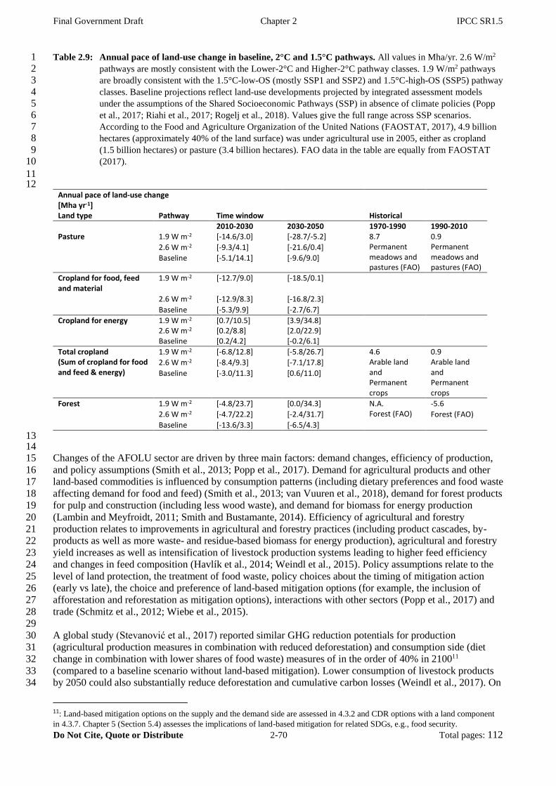
Final Government Draft Chapter 2 IPCC SR1.5
Do Not Cite, Quote or Distribute 2-70 Total pages: 112
Table 2.9: Annual pace of land-use change in baseline, 2°C and 1.5°C pathways. All values in Mha/yr. 2.6 W/m2 1 pathways are mostly consistent with the Lower-2°C and Higher-2°C pathway classes. 1.9 W/m2 pathways 2 are broadly consistent with the 1.5°C-low-OS (mostly SSP1 and SSP2) and 1.5°C-high-OS (SSP5) pathway 3 classes. Baseline projections reflect land-use developments projected by integrated assessment models 4 under the assumptions of the Shared Socioeconomic Pathways (SSP) in absence of climate policies (Popp 5 et al., 2017; Riahi et al., 2017; Rogelj et al., 2018). Values give the full range across SSP scenarios. 6 According to the Food and Agriculture Organization of the United Nations (FAOSTAT, 2017), 4.9 billion 7 hectares (approximately 40% of the land surface) was under agricultural use in 2005, either as cropland 8 (1.5 billion hectares) or pasture (3.4 billion hectares). FAO data in the table are equally from FAOSTAT 9 (2017). 10
11 12
Annual pace of land-use change [Mha yr-1]
Land type Pathway Time window Historical
2010-2030 2030-2050 1970-1990 1990-2010 Pasture 1.9 W m-2 [-14.6/3.0] [-28.7/-5.2] 8.7
Permanent meadows and pastures (FAO)
0.9 Permanent meadows and pastures (FAO)
2.6 W m-2 [-9.3/4.1] [-21.6/0.4]
Baseline [-5.1/14.1] [-9.6/9.0]
Cropland for food, feed and material
1.9 W m-2 [-12.7/9.0] [-18.5/0.1]
2.6 W m-2 [-12.9/8.3] [-16.8/2.3]
Baseline [-5.3/9.9] [-2.7/6.7]
Cropland for energy 1.9 W m-2 [0.7/10.5] [3.9/34.8] 2.6 W m-2 [0.2/8.8] [2.0/22.9] Baseline [0.2/4.2] [-0.2/6.1]
Total cropland (Sum of cropland for food and feed & energy)
1.9 W m-2 [-6.8/12.8] [-5.8/26.7] 4.6 Arable land and Permanent crops
0.9 Arable land and Permanent crops
2.6 W m-2 [-8.4/9.3] [-7.1/17.8]
Baseline [-3.0/11.3] [0.6/11.0]
Forest 1.9 W m-2 [-4.8/23.7] [0.0/34.3] N.A. Forest (FAO)
-5.6
2.6 W m-2 [-4.7/22.2] [-2.4/31.7] Forest (FAO)
Baseline [-13.6/3.3] [-6.5/4.3]
13 14 Changes of the AFOLU sector are driven by three main factors: demand changes, efficiency of production, 15
and policy assumptions (Smith et al., 2013; Popp et al., 2017). Demand for agricultural products and other 16
land-based commodities is influenced by consumption patterns (including dietary preferences and food waste 17
affecting demand for food and feed) (Smith et al., 2013; van Vuuren et al., 2018), demand for forest products 18
for pulp and construction (including less wood waste), and demand for biomass for energy production 19
(Lambin and Meyfroidt, 2011; Smith and Bustamante, 2014). Efficiency of agricultural and forestry 20
production relates to improvements in agricultural and forestry practices (including product cascades, by-21
products as well as more waste- and residue-based biomass for energy production), agricultural and forestry 22
yield increases as well as intensification of livestock production systems leading to higher feed efficiency 23
and changes in feed composition (Havlík et al., 2014; Weindl et al., 2015). Policy assumptions relate to the 24
level of land protection, the treatment of food waste, policy choices about the timing of mitigation action 25
(early vs late), the choice and preference of land-based mitigation options (for example, the inclusion of 26
afforestation and reforestation as mitigation options), interactions with other sectors (Popp et al., 2017) and 27
trade (Schmitz et al., 2012; Wiebe et al., 2015). 28
29
A global study (Stevanović et al., 2017) reported similar GHG reduction potentials for production 30
(agricultural production measures in combination with reduced deforestation) and consumption side (diet 31
change in combination with lower shares of food waste) measures of in the order of 40% in 210011 32
(compared to a baseline scenario without land-based mitigation). Lower consumption of livestock products 33
by 2050 could also substantially reduce deforestation and cumulative carbon losses (Weindl et al., 2017). On 34
11: Land-based mitigation options on the supply and the demand side are assessed in 4.3.2 and CDR options with a land component
in 4.3.7. Chapter 5 (Section 5.4) assesses the implications of land-based mitigation for related SDGs, e.g., food security.
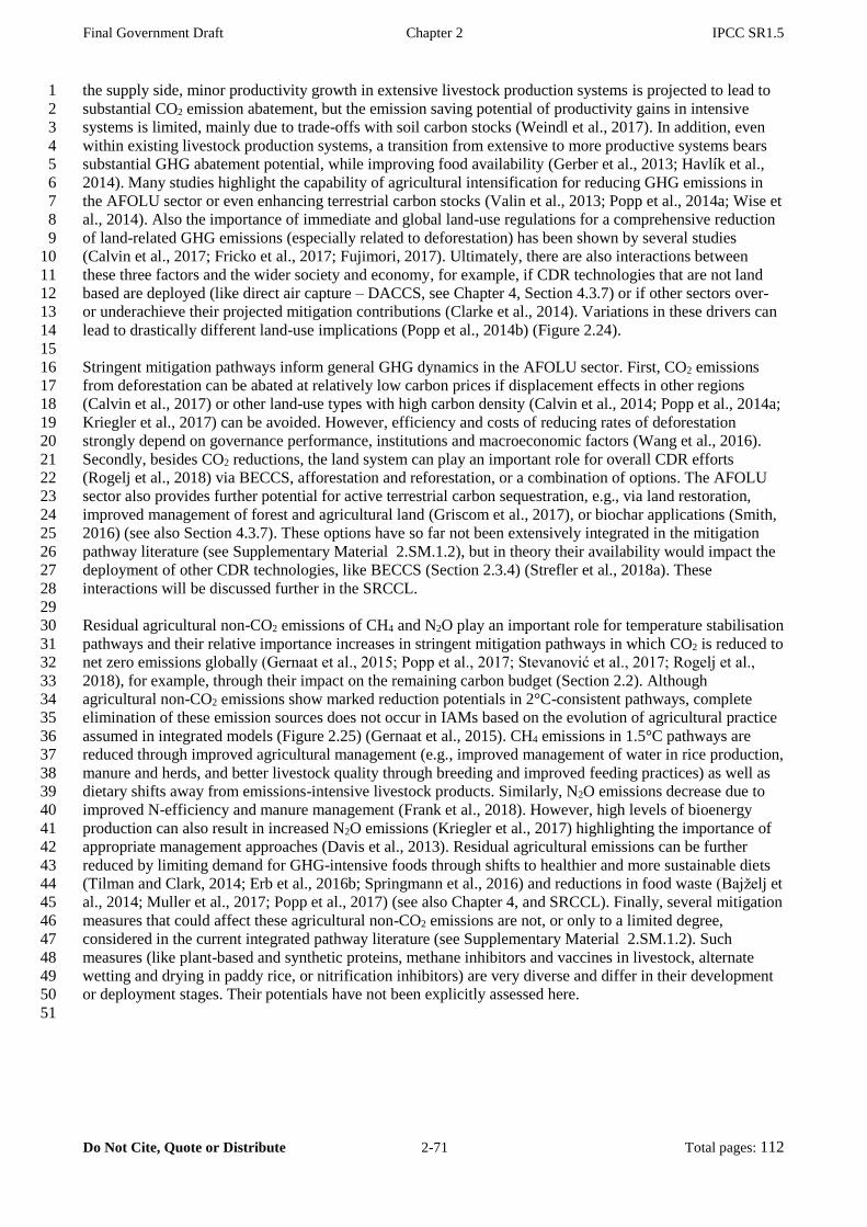
Final Government Draft Chapter 2 IPCC SR1.5
Do Not Cite, Quote or Distribute 2-71 Total pages: 112
the supply side, minor productivity growth in extensive livestock production systems is projected to lead to 1
substantial CO2 emission abatement, but the emission saving potential of productivity gains in intensive 2
systems is limited, mainly due to trade-offs with soil carbon stocks (Weindl et al., 2017). In addition, even 3
within existing livestock production systems, a transition from extensive to more productive systems bears 4
substantial GHG abatement potential, while improving food availability (Gerber et al., 2013; Havlík et al., 5
2014). Many studies highlight the capability of agricultural intensification for reducing GHG emissions in 6
the AFOLU sector or even enhancing terrestrial carbon stocks (Valin et al., 2013; Popp et al., 2014a; Wise et 7
al., 2014). Also the importance of immediate and global land-use regulations for a comprehensive reduction 8
of land-related GHG emissions (especially related to deforestation) has been shown by several studies 9
(Calvin et al., 2017; Fricko et al., 2017; Fujimori, 2017). Ultimately, there are also interactions between 10
these three factors and the wider society and economy, for example, if CDR technologies that are not land 11
based are deployed (like direct air capture – DACCS, see Chapter 4, Section 4.3.7) or if other sectors over- 12
or underachieve their projected mitigation contributions (Clarke et al., 2014). Variations in these drivers can 13
lead to drastically different land-use implications (Popp et al., 2014b) (Figure 2.24). 14
15
Stringent mitigation pathways inform general GHG dynamics in the AFOLU sector. First, CO2 emissions 16
from deforestation can be abated at relatively low carbon prices if displacement effects in other regions 17
(Calvin et al., 2017) or other land-use types with high carbon density (Calvin et al., 2014; Popp et al., 2014a; 18
Kriegler et al., 2017) can be avoided. However, efficiency and costs of reducing rates of deforestation 19
strongly depend on governance performance, institutions and macroeconomic factors (Wang et al., 2016). 20
Secondly, besides CO2 reductions, the land system can play an important role for overall CDR efforts 21
(Rogelj et al., 2018) via BECCS, afforestation and reforestation, or a combination of options. The AFOLU 22
sector also provides further potential for active terrestrial carbon sequestration, e.g., via land restoration, 23
improved management of forest and agricultural land (Griscom et al., 2017), or biochar applications (Smith, 24
2016) (see also Section 4.3.7). These options have so far not been extensively integrated in the mitigation 25
pathway literature (see Supplementary Material 2.SM.1.2), but in theory their availability would impact the 26
deployment of other CDR technologies, like BECCS (Section 2.3.4) (Strefler et al., 2018a). These 27
interactions will be discussed further in the SRCCL. 28
29
Residual agricultural non-CO2 emissions of CH4 and N2O play an important role for temperature stabilisation 30
pathways and their relative importance increases in stringent mitigation pathways in which CO2 is reduced to 31
net zero emissions globally (Gernaat et al., 2015; Popp et al., 2017; Stevanović et al., 2017; Rogelj et al., 32
2018), for example, through their impact on the remaining carbon budget (Section 2.2). Although 33
agricultural non-CO2 emissions show marked reduction potentials in 2°C-consistent pathways, complete 34
elimination of these emission sources does not occur in IAMs based on the evolution of agricultural practice 35
assumed in integrated models (Figure 2.25) (Gernaat et al., 2015). CH4 emissions in 1.5°C pathways are 36
reduced through improved agricultural management (e.g., improved management of water in rice production, 37
manure and herds, and better livestock quality through breeding and improved feeding practices) as well as 38
dietary shifts away from emissions-intensive livestock products. Similarly, N2O emissions decrease due to 39
improved N-efficiency and manure management (Frank et al., 2018). However, high levels of bioenergy 40
production can also result in increased N2O emissions (Kriegler et al., 2017) highlighting the importance of 41
appropriate management approaches (Davis et al., 2013). Residual agricultural emissions can be further 42
reduced by limiting demand for GHG-intensive foods through shifts to healthier and more sustainable diets 43
(Tilman and Clark, 2014; Erb et al., 2016b; Springmann et al., 2016) and reductions in food waste (Bajželj et 44
al., 2014; Muller et al., 2017; Popp et al., 2017) (see also Chapter 4, and SRCCL). Finally, several mitigation 45
measures that could affect these agricultural non-CO2 emissions are not, or only to a limited degree, 46
considered in the current integrated pathway literature (see Supplementary Material 2.SM.1.2). Such 47
measures (like plant-based and synthetic proteins, methane inhibitors and vaccines in livestock, alternate 48
wetting and drying in paddy rice, or nitrification inhibitors) are very diverse and differ in their development 49
or deployment stages. Their potentials have not been explicitly assessed here. 50
51
Final Government Draft Chapter 2 IPCC SR1.5
Do Not Cite, Quote or Distribute 2-72 Total pages: 112
1 Figure 2.25: Agricultural emissions in transformation pathways. Global agricultural CH4 (left) and N2O (right) 2
emissions. Boxplots show median, interquartile range and full range. Classes are defined in Section 2.1. 3 4
Pathways consistent with 1.5°C rely on one or more of the three strategies highlighted above (demand 5
changes, efficiency gains, and policy assumptions), and can apply these in different configurations. For 6
example, among the four illustrative archetypes used in this chapter (Section 2.1) the LED and S1 pathways 7
focus on generally low resource and energy consumption (including healthy diets with low animal-calorie 8
shares and low food waste) as well as significant agricultural intensification in combination with high levels 9
of nature protection. Under such assumptions, comparably small amounts of land are needed for land 10
demanding mitigation activities such as BECCS and afforestation and reforestation, leaving the land 11
footprint for energy crops in 2050 virtually the same compared to 2010 levels for the LED pathway. In 12
contrast, future land-use developments can look very differently under the resource- and energy-intensive S5 13
pathway that includes unhealthy diets with high animal shares and high shares of food waste (Tilman and 14
Clark, 2014; Springmann et al., 2016) combined with a strong orientation towards technology solutions to 15
compensate for high reliance on fossil-fuel resources and associated high levels of GHG emissions in the 16
baseline. In such pathways, climate change mitigation strategies strongly depend on the availability of CDR 17
through BECCS (Humpenöder et al., 2014). As a consequence, the S5 pathway sources significant amounts 18
of biomass through bioenergy crop expansion in combination with agricultural intensification. Also, further 19
policy assumptions can strongly affect land-use developments, highlighting the importance for land use of 20
making appropriate policy choices. For example, within the SSP set, some pathways rely strongly on a 21
policy to incentivise afforestation and reforestation for CDR together with BECCS, which results in an 22
expansion of forest area and a corresponding increase in terrestrial carbon stock. Finally, the variety of 23
pathways illustrates how policy choices in the AFOLU and other sectors strongly affect land-use 24
developments and associated sustainable development interactions (Section 5.4) in 1.5°C pathways. 25
26
The choice of strategy or mitigation portfolio impacts the GHG dynamics of the land system and other 27
sectors (see Section 2.3), as well as the synergies and trade-offs with other environmental and societal 28
objectives (see Section 2.5.3 and Section 5.4). For example, AFOLU developments in 1.5°C pathways range 29
from strategies that differ almost an order of magnitude in their projected land requirements for bioenergy 30
(Figure 2.24), and some strategies would allow an increase in forest cover over the 21st century compared to 31
strategies under which forest cover remains approximately constant. High agricultural yields and application 32
of intensified animal husbandry, implementation of best-available technologies for reducing non-CO2 33
emissions, or lifestyle changes including a less-meat-intensive diet and less CO2-intensive transport modes, 34
have been identified to allow for such a forest expansion and reduced footprints from bioenergy without 35
compromising food security (Frank et al., 2017; Doelman et al., 2018; van Vuuren et al., 2018). 36
37
The IAMs used in the pathways underlying this assessment (Popp et al., 2017; Riahi et al., 2017; Rogelj et 38
al., 2018) do not include all potential land-based mitigation options and side-effects, and their results are 39
hence subject to uncertainty. For example, recent research has highlighted the potential impact of forest 40
management practices on land carbon content (Erb et al., 2016a; Naudts et al., 2016) and the uncertainty 41
surrounding future crop yields (Haberl et al., 2013; Searle and Malins, 2014), and water availability (Liu et 42
al., 2014). These aspects are included in IAMs in varying degrees, but were not assessed in this report. 43
Furthermore, land-use modules of some IAMs can depict spatially resolved climate damages to agriculture 44
(Nelson et al., 2014), but this option was not used in the SSP quantifications (Riahi et al., 2017). Damages 45
(e.g., due to ozone exposure or varying indirect fertilization due to atmospheric N and Fe deposition (e.g., 46
Final Government Draft Chapter 2 IPCC SR1.5
Do Not Cite, Quote or Distribute 2-73 Total pages: 112
Shindell et al., 2012; Mahowald et al., 2017) are also not included. Finally, this assessment did not look into 1
the literature of agricultural sector models which could provide important additional detail and granularity to 2
the here presented discussion12. This limits their ability to capture the full mitigation potentials and benefits 3
between scenarios. An in-depth assessment of these aspects lies outside the scope of this Special Report. 4
However, their existence affects the confidence assessment of the AFOLU transition in 1.5°C pathways. 5
6
Despite the limitations of current modelling approaches, there is high agreement and robust evidence across 7
models and studies that the AFOLU sector plays an important role in stringent mitigation pathways. The 8
findings from these multiple lines of evidence also result in high confidence that AFOLU mitigation 9
strategies can vary significantly based on preferences and policy choices, facilitating the exploration of 10
strategies that can achieve multiple societal objectives simultaneously (see also Section 2.5.3). At the same 11
time, given the many uncertainties and limitations, only low to medium confidence can be attributed by this 12
assessment to the more extreme AFOLU developments found in the pathway literature, and low to medium 13
confidence to the level of residual non-CO2 emissions. 14
12: For example, the GLEAM (http://www.fao.org/gleam/en/) model from the UN Food and Agricultural Organisation (FAO).
Final Government Draft Chapter 2 IPCC SR1.5
Do Not Cite, Quote or Distribute 2-74 Total pages: 112
2.5 Challenges, opportunities and co-impacts of transformative mitigation pathways 1
2
This section examines aspects other than climate outcomes of 1.5°C mitigation pathways. Focus is given to 3
challenges and opportunities related to policy regimes, price of carbon and co-impacts, including sustainable 4
development issues, which can be derived from the existing integrated pathway literature. Attention is also 5
given to uncertainties and critical assumptions underpinning mitigation pathways. The challenges and 6
opportunities identified in this section are further elaborated Chapter 4 (e.g., policy choice and 7
implementation) and Chapter 5 (e.g., sustainable development). The assessment indicates unprecedented 8
policy and geopolitical challenges. 9
10
11
2.5.1 Policy frameworks and enabling conditions 12
13
Moving from a 2°C to a 1.5°C pathway implies bold integrated policies that enable higher socio-technical 14
transition speeds, larger deployment scales, and the phase-out of existing systems that may lock in emissions 15
for decades (Geels et al., 2017; Kuramochi et al., 2017; Rockström et al., 2017; Vogt-Schilb and Hallegatte, 16
2017; Kriegler et al., 2018b; Michaelowa et al., 2018) (high confidence). This requires higher levels of 17
transformative policy regimes in the near term, which allow deep decarbonisation pathways to emerge and a 18
net zero carbon energy-economy system to emerge in the 2040–2060 period (Rogelj et al., 2015b; Bataille et 19
al., 2016b). This enables accelerated levels of technological deployment and innovation (Geels et al., 2017; 20
IEA, 2017a; Grubler et al., 2018) and assumes more profound behavioural, economic and political 21
transformation (Sections 2.3, 2.4 and 4.4). Despite inherent levels of uncertainty attached to modelling 22
studies (e.g., related to climate and carbon-cycle response), studies stress the urgency for transformative 23
policy efforts to reduce emissions in the short term (Riahi et al., 2015; Kuramochi et al., 2017; Rogelj et al., 24
2018). 25
26
The available literature indicates that mitigation pathways in line with 1.5°C-consistent pathways would 27
require stringent and integrated policy interventions (very high confidence). Higher policy ambition often 28
takes the form of stringent economy-wide emission targets (and resulting peak-and-decline of emissions), 29
larger coverage of NDCs to more gases and sectors (e.g., land-use, international aviation), much lower 30
energy and carbon intensity rates than historically seen, carbon prices much higher than the ones observed in 31
real markets, increased climate finance, global coordinated policy action, and implementation of additional 32
initiatives (e.g., by non-state actors) (Sections 2.3, 2.4 and 2.5.2). The diversity (beyond carbon pricing) and 33
effectiveness of policy portfolios are of prime importance, particularly in the short-term (Mundaca and 34
Markandya, 2016; Kuramochi et al., 2017; OECD, 2017; Kriegler et al., 2018b; Michaelowa et al., 2018). 35
For instance, deep decarbonisation pathways in line with a 2˚C target (covering 74% of global energy-system 36
emissions) include a mix of stringent regulation (e.g., building codes, minimum performance standards), 37
carbon pricing mechanisms and R&D (research and development) innovation policies (Bataille et al., 2016a). 38
Carbon pricing, direct regulation and public investment to enable innovation are critical for deep 39
decarbonisation pathways (Grubb et al., 2014). Effective planning (including compact city measures) and 40
integrated regulatory frameworks are also key drivers in the IEA-ETP B2DS study for the transport sector 41
(IEA, 2017a). Effective urban planning can reduce GHG emissions from urban transport between 20% and 42
50% (Creutzig, 2016). Comprehensive policy frameworks would be needed if the decarbonisation of the 43
power system is pursued while increasing end-use electrification (including transport) (IEA, 2017a). 44
Technology policies (e.g., feed-in-tariffs), financing instruments, carbon pricing and system integration 45
management driving the rapid adoption of renewable energy technologies are critical for the decarbonisation 46
of electricity generation (Bruckner et al., 2014; Luderer et al., 2014; Creutzig et al., 2017; Pietzcker et al., 47
2017). Likewise, low-carbon and resilient investments are facilitated by a mix of coherent policies including 48
fiscal and structural reforms (e.g., labour markets), public procurement, carbon pricing, stringent standards, 49
information schemes, technology policies, fossil-fuel subsidy removal, climate risk disclosure, and land-use 50
and transport planning (OECD, 2017). Pathways in which CDR options are restricted emphasise the 51
strengthening of near-term policy mixes (Luderer et al., 2013; Kriegler et al., 2018b). Together with the 52
decarbonisation of the supply side, ambitious policies targeting fuel switching and energy efficiency 53
improvements on the demand side play a major role across mitigation pathways (Clarke et al., 2014; Kriegler 54
et al., 2014b; Riahi et al., 2015; Kuramochi et al., 2017; Brown and Li, 2018; Rogelj et al., 2018; 55
Wachsmuth and Duscha, 2018). 56
57

Final Government Draft Chapter 2 IPCC SR1.5
Do Not Cite, Quote or Distribute 2-75 Total pages: 112
The combined evidence suggests that aggressive policies addressing energy efficiency are central in keeping 1
1.5°C within reach and lowering energy system and mitigation costs (Luderer et al., 2013; Rogelj et al., 2
2013b, 2015b; Grubler et al., 2018) (high confidence). Demand-side policies that increase energy efficiency 3
or limit energy demand at a higher rate than historically observed are critical enabling factors reducing 4
mitigation costs for stringent mitigation pathways across the board (Luderer et al., 2013; Rogelj et al., 2013b, 5
2015b; Clarke et al., 2014; Bertram et al., 2015a; Bataille et al., 2016b). Ambitious sector-specific mitigation 6
policies in industry, transportation and residential sectors are needed in the short run for emissions to peak in 7
2030 (Méjean et al., 2018). Stringent demand-side policies (e.g., tightened efficiency standards for buildings 8
and appliances) driving the expansion, efficiency and provision of high-quality energy services are essential 9
to meet a 1.5˚C mitigation target while avoiding the need of CDR (Grubler et al., 2018). A 1.5˚C pathway for 10
the transport sector is possible using a mix of additional and stringent policy actions preventing (or reducing) 11
the need for transport, encouraging shifts towards efficient modes of transport, and improving vehicle-fuel 12
efficiency (Ghota et al., 2018). Stringent demand-side policies also reduce the need for CCS (Wachsmuth 13
and Duscha, 2018). Even in the presence of weak-near term policy frameworks, increased energy efficiency 14
lowers mitigation costs noticeably compared to pathways with reference energy intensity (Bertram et al., 15
2015a). Horizontal issues in the literature relate to the rebound effect, the potential overestimation of the 16
effectiveness of energy efficiency policy, and policies to counteract the rebound (Saunders, 2015; van den 17
Bergh, 2017; Grubler et al., 2018) (Sections 2.4 and 4.4). 18
19
SSP-based modelling studies underline that socio-economic and climate policy assumptions strongly 20
influence mitigation pathway characteristics and the economics of achieving a specific climate target (Bauer 21
et al., 2017; Guivarch and Rogelj, 2017; Riahi et al., 2017; Rogelj et al., 2018) (very high confidence). SSP 22
assumptions related to economic growth and energy intensity are critical determinants of projected CO2 23
emissions (Marangoni et al., 2017). A multi-model inter-comparison study found that mitigation challenges 24
in line with a 1.5˚C target vary substantially across SSPs and policy assumptions (Rogelj et al., 2018). Under 25
SSP1-SPA1 (sustainability) and SSP2-SPA2 (middle-of-the-road), the majority of IAMs were capable of 26
producing 1.5˚C pathways. On the contrary, none of the IAMs contained in the SR1.5 database could 27
produce a 1.5°C pathway under SSP3-SPA3 assumptions. Preventing elements include, for instance, climate 28
policy fragmentation, limited control of land-use emissions, heavy reliance on fossil fuels, unsustainable 29
consumption and marked inequalities (Rogelj et al., 2018). Dietary aspects of the SSPs are also critical: 30
climate-friendly diets were contained in ‘sustainability’ (SSP1) and meat-intensive diets in SSP3 and SSP5 31
(Popp et al., 2017). CDR requirements are reduced under ‘sustainability’ related assumptions (Strefler et al., 32
2018b). These are major policy-related factors for why SSP1-SPA1 translates into relatively low mitigation 33
challenges whereas SSP3-SPA3 and SSP5-SPA5 entail futures that pose the highest socio-technical and 34
economic challenges. SSPs/SPAs assumptions indicate that policy-driven pathways that encompass 35
accelerated change away from fossil fuels, large-scale deployment of low-carbon energy supplies, improved 36
energy efficiency and sustainable consumption lifestyles reduce the risks of climate targets becoming 37
unreachable (Clarke et al., 2014; Riahi et al., 2015, 2017; Marangoni et al., 2017; Rogelj et al., 2017, 2018; 38
Strefler et al., 2018b). 39
40
Policy assumptions that lead to weak or delayed mitigation action from what would be possible in a fully 41
cooperative world, strongly influence the achievability of mitigation targets (Luderer et al., 2013; Rogelj et 42
al., 2013; OECD, 2017; Holz et al., 2018a; Strefler et al., 2018b) (high confidence). Such regimes also 43
include current NDCs (Fawcett et al., 2015; Aldy et al., 2016; Rogelj et al., 2016a, 2017; Hof et al., 2017; 44
van Soest et al., 2017), which have been reported to make achieving a 2°C pathway unattainable without 45
CDR (Strefler et al., 2018b). Not strengthening NDCs make it very challenging to keep 1.5°C within reach 46
(see Section 2.3 and Cross-Chapter Box 11 in Chapter 4). One multi-model inter-comparison study (Luderer 47
et al., 2016b, 2018) explored the effects on 1.5°C pathways assuming the implementation of current NDCs 48
until 2030 and stringent reductions thereafter. It finds that delays in globally coordinated actions leads to 49
various models reaching no 1.5°C-consistent pathways during the 21st century. Transnational emission 50
reduction initiatives (TERIs) outside the UNFCCC have also been assessed and found to overlap (70–80%) 51
with NDCs and be inadequate to bridge the gap between NDCs and a 2˚C pathway (Roelfsema et al., 2018). 52
Weak and fragmented short-term policy efforts use up a large share of the long-term carbon budget before 53
2030–2050 (Bertram et al., 2015a; van Vuuren et al., 2016) and increase the need for the full portfolio of 54
mitigation measures, including CDR (Clarke et al., 2014; Riahi et al., 2015; Xu and Ramanathan, 2017). 55
Furthermore, fragmented policy scenarios also exhibit ‘carbon leakage’ via energy and capital markets 56
(Arroyo-Currás et al., 2015; Kriegler et al., 2015b). A lack of integrated policy portfolios can increase the 57

Final Government Draft Chapter 2 IPCC SR1.5
Do Not Cite, Quote or Distribute 2-76 Total pages: 112
risks of trade-offs between mitigation approaches and sustainable development objectives (see Sections 2.5.3 1
and 5.4). However, more detailed analysis is needed about realistic (less disruptive) policy trajectories until 2
2030 that can strengthen near-term mitigation action and meaningfully decrease post-2030 challenges (see 3
Section 4.4). 4
5
Whereas the policy frameworks and enabling conditions identified above pertain to the ‘idealised’ dimension 6
of mitigation pathways, aspects related to 1.5°C mitigation pathways in practice are of prime importance. For 7
example, issues related to second-best stringency levels, international cooperation, public acceptance, 8
distributional consequences, multi-level governance, non-state actions, compliance levels, capacity building, 9
rebound effects, linkages across highly heterogeneous policies, sustained behavioural change, finance and 10
intra- and inter-generational issues need to be considered (Somanthan et al., 2014; Bataille et al., 2016a; 11
Mundaca and Markandya, 2016; Baranzini et al., 2017; van den Bergh, 2017; Vogt-Schilb and Hallegatte, 12
2017; Chan et al., 2018; Holz et al., 2018a; Klinsky and Winkler, 2018; Michaelowa et al., 2018; Patterson et 13
al., 2018) (see Section 4.4). Furthermore, policies interact with a wide portfolio of pre-existing policy 14
instruments that address multiple areas (e.g., technology markets, economic growth, poverty alleviation, 15
climate adaptation) and deal with various market failures (e.g., information asymmetries) and behavioural 16
aspects (e.g., heuristics) that prevent or hinder mitigation actions (Kolstad et al., 2014; Mehling and 17
Tvinnereim, 2018). The socio-technical transition literature points to multiple complexities in real-world 18
settings that prevent reaching ‘idealised’ policy conditions but at the same time can still accelerate 19
transformative change through other co-evolutionary processes of technology and society (Geels et al., 2017; 20
Rockström et al., 2017). Such co-processes are complex and go beyond the role of policy (including carbon 21
pricing) and comprise the role of citizens, businesses, stakeholder groups or governments, as well as the 22
interplay of institutional and socio-political dimensions (Michaelowa et al., 2018; Veland et al., 2018). It is 23
argued that large system transformations, similar to those in 1.5°C pathways, require prioritizing an 24
evolutionary and behavioural framework in economic theory rather than an optimization or equilibrium 25
framework as is common in current IAMs (Grubb et al., 2014; Patt, 2017). Accumulated know-how, 26
accelerated innovation and public investment play a key role in (rapid) transitions (Geels et al., 2017; 27
Michaelowa et al., 2018) (see Sections 4.2 and 4.4). 28
29
In summary, the emerging literature supports the AR5 on the need for integrated, robust and stringent policy 30
frameworks targeting both the supply and demand-side of energy-economy systems (high confidence). 31
Continuous ex-ante policy assessments provide learning opportunities for both policy makers and 32
stakeholders. 33
34
[START CROSS CHAPTER BOX 5 HERE] 35
Cross-Chapter Box 5: Economics of 1.5°C Pathways and the Social Cost of Carbon 36
37
Luis Mundaca (Sweden/Chile), Mustafa Babiker (Sudan), Johannes Emmerling (Germany/Italy), Sabine 38
Fuss (Germany), Jean-Charles Hourcade (France), Elmar Kriegler (Germany), Anil Markandya (UK/Spain), 39
Joyashree Roy (India), Drew Shindell (USA) 40
41
Two approaches have been commonly used to assess alternative emissions pathways: cost-effectiveness 42
analysis (CEA) and cost-benefit analysis (CBA). CEA aims at identifying emissions pathways minimising 43
the total mitigation costs of achieving a given warming or GHG limit (Clarke et al., 2014). CBA has the goal 44
to identify the optimal emissions trajectory minimising the discounted flows of abatement expenditures and 45
monetised climate change damages (Boardman, 2006; Stern, 2007). A third concept, the Social Cost of 46
Carbon (SCC) measures the total net damages of an extra metric ton of CO2 emissions due to the associated 47
climate change (Nordhaus, 2014; Pizer et al., 2014; Rose et al., 2017a). Negative and positive impacts are 48
monetised, discounted and the net value is expressed as an equivalent loss of consumption today. The SCC 49
can be evaluated for any emissions pathway under policy consideration (Rose, 2012; NASEM, 2016, 2017). 50
51
Along the optimal trajectory determined by CBA, the SCC equals the discounted value of the marginal 52
abatement cost of a metric ton of CO2 emissions. Equating the present value of future damages and marginal 53
abatement costs includes a number of critical value judgments in the formulation of the social welfare 54
function (SWF), particularly in how non-market damages and the distribution of damages across countries 55
and individuals and between current and future generations are valued (Kolstad et al., 2014). For example, 56
since climate damages accrue to a larger extent in the farther future and can persist for many years, 57
Final Government Draft Chapter 2 IPCC SR1.5
Do Not Cite, Quote or Distribute 2-77 Total pages: 112
assumptions and approaches to determine the social discount rate (normative ‘prescriptive’ vs. positive 1
‘descriptive’) and social welfare function (e.g., discounted utilitarian SWF vs. undiscounted prioritarian 2
SWF) can heavily influence CBA outcomes and associated estimates of SCC (Kolstad et al., 2014; Pizer et 3
al., 2014; Adler and Treich, 2015; Adler et al., 2017; NASEM, 2017; Nordhaus, 2017; Rose et al., 2017a). 4
5
In CEA, the marginal abatement cost of carbon is determined by the climate goal under consideration. It 6
equals the shadow price of carbon associated with the goal which in turn can be interpreted as the 7
willingness to pay for imposing the goal as a political constraint. Emissions prices are usually expressed in 8
carbon (equivalent) prices using the GWP-100 metric as the exchange rate for pricing emissions of non-CO2 9
GHGs controlled under internationally climate agreements (like CH4, N2O and fluorinated gases, see Cross-10
Chapter Box 1.2)13. Since policy goals like the goals of limiting warming to 1.5°C or well below 2°C do not 11
directly result from a money metric trade-off between mitigation and damages, associated shadow prices can 12
differ from the SCC in a CBA. In CEA, value judgments are to a large extent concentrated in the choice of 13
climate goal and related implications, while more explicit assumptions about social values are required to 14
perform CBA. For example, assumptions about the social discount rate no longer affect the overall 15
abatement levels now set by the climate goal, but the choice and timing of investments in individual 16
measures to reach these levels. 17
18
Although CBA-based and CEA-based assessment are both subject to large uncertainty about socio-techno-19
economic trends, policy developments and climate response, the range of estimates for the SCC along an 20
optimal trajectory determined by CBA is far higher than for estimates of the shadow price of carbon in CEA-21
based approaches. In CBA, the value judgments about inter- and intra-generational equity combined with 22
uncertainties in the climate damage functions assumed, including their empirical basis, are important 23
(Pindyck, 2013; Stern, 2013; Revesz et al., 2014). In a CEA-based approach, the value judgments about the 24
aggregate welfare function matter less and uncertainty about climate response and impacts can be tied into 25
various climate targets and related emissions budgets (Clarke et al., 2014). 26
27
The CEA- and CBA-based carbon cost estimates are derived with a different set of tools. They are all 28
summarised as integrated assessment models (IAMs) but in fact are of very different nature (Weyant, 2017). 29
Detailed process IAMs such as AIM (Fujimori, 2017), GCAM (Thomson et al., 2011; Calvin et al., 2017), 30
IMAGE (van Vuuren et al., 2011b, 2017b), MESSAGE-GLOBIOM (Riahi et al., 2011; Havlík et al., 2014; 31
Fricko et al., 2017), REMIND-MAgPIE (Popp et al., 2010; Luderer et al., 2013; Kriegler et al., 2017) and 32
WITCH (Bosetti et al., 2006, 2008, 2009) include a process-based representation of energy and land systems, 33
but in most cases lack a comprehensive representation of climate damages, and are typically used for CEA. 34
Diagnostic analyses across CBA-IAMs indicate important dissimilarities in modelling assembly, 35
implementation issues and behaviour (e.g., parametric uncertainty, damage responses, income sensitivity) 36
that need to be recognised to better understand SCC estimates (Rose et al., 2017a). 37
38
CBA-IAMs such as DICE (Nordhaus and Boyer, 2000; Nordhaus, 2013, 2017), PAGE (Hope, 2006) and 39
FUND (Tol, 1999; Anthoff and Tol, 2009) attempt to capture the full feedback from climate response to 40
socio-economic damages in an aggregated manner, but are usually much more stylised than detailed process 41
IAMs. In a nutshell, the methodological framework for estimating SCC involves projections of population 42
growth, economic activity and resulting emissions; computations of atmospheric composition and global-43
mean temperatures as a result of emissions; estimations of physical impacts of climate changes; monetisation 44
of impacts (positive and negative) on human welfare; and the discounting of the future monetary value of 45
impacts to year of emission (Kolstad et al., 2014; Revesz et al., 2014; NASEM, 2017; Rose et al., 2017a). 46
There has been a discussion in the literature to what extent CBA-IAMs underestimate the SCC due to, for 47
example, a limited treatment or difficulties in addressing damages to human well-being, labour productivity, 48
value of capital stock, ecosystem services and the risks of catastrophic climate change for future generations 49
(Ackerman and Stanton, 2012; Revesz et al., 2014; Moore and Diaz, 2015; Stern, 2016). However, there has 50
been progress in ‘bottom-up’ empirical analyses of climate damages (Hsiang et al., 2017), the insights of 51
which could be integrated into these models (Dell et al., 2014). Most of the models used in Chapter 2 on 52
1.5°C mitigation pathways are detailed process IAMs and thus deal with CEA. 53
54
13: Also other metrics to compare emissions have been suggested and adopted by governments nationally (Kandlikar, 1995; Marten
et al., 2015; Shindell, 2015; Interagency Working Group on Social Cost of Greenhouse Gases, 2016).

Final Government Draft Chapter 2 IPCC SR1.5
Do Not Cite, Quote or Distribute 2-78 Total pages: 112
An important question is how results from CEA- and CBA-type approaches can be compared and 1
synthesised. Such synthesis needs to be done with care, since estimates of the shadow price of carbon under 2
the climate goal and SCC estimates from CBA might not be directly comparable due to different tools, 3
approaches and assumptions used to derive them. Acknowledging this caveat, the SCC literature has 4
identified a range of factors, assumptions and value judgements that support SCC values above $100 tCO2–1 5
that are also found as net present values of the shadow price of carbon in 1.5°C pathways. These factors 6
include accounting for tipping points in the climate system (Lemoine and Traeger, 2014; Cai et al., 2015; 7
Lontzek et al., 2015), a low social discount rate (Nordhaus, 2005; Stern, 2007) and inequality aversion 8
(Schmidt et al., 2013; Dennig et al., 2015; Adler et al., 2017). 9
10
The SCC and the shadow price of carbon are not merely theoretical concepts but used in regulation (Pizer et 11
al., 2014; Revesz et al., 2014; Stiglitz et al., 2017). As stated by the report of the High-Level Commission on 12
Carbon Pricing (Stiglitz et al., 2017), in the real world there is a distinction to be made between the 13
implementable and efficient explicit carbon prices and the implicit (notional) carbon prices to be retained for 14
policy appraisal and the evaluation of public investments, as is already done in some jurisdictions such as the 15
USA, UK and France. Since 2008, the U.S. government has used SCC estimates to assess the benefits and 16
costs related to CO2 emissions resulting from federal policymaking (NASEM, 2017; Rose et al., 2017a). 17
18
The use of the SCC for policy appraisals is however not straightforward in an SDG context. There are 19
suggestions that a broader range of polluting activities than only CO2 emissions, for example emissions of air 20
pollutants, and a broader range of impacts than only climate change, such as impacts on air quality, health 21
and sustainable development in general (see Chapter 5 for a detailed discussion), would need to be included 22
in social costs (Sarofim et al., 2017; Shindell et al., 2017a). Most importantly, a consistent valuation of the 23
SCC in a sustainable development framework would require accounting for the SDGs in the social welfare 24
formulation (see Chapter 5). 25
[END CROSS CHAPTER BOX 5 HERE] 26 27
28
2.5.2 Economic and financial implications of 1.5°C Pathways 29
30
Price of carbon emissions 31
32
The price of carbon assessed here is fundamentally different from the concepts of optimal carbon price in a 33
cost-benefit analysis, or the social cost of carbon (see Cross-Chapter Box 5 in this Chapter and Section 34
3.5.2). Under a cost-effective analysis (CEA) modelling framework, prices for carbon (mitigation costs) 35
reflect the stringency of mitigation requirements at the margin (i.e., cost of mitigating one extra unit of 36
emission). 37
38
Based on data available for this special report, the price of carbon varies substantially across models and 39
scenarios, and their value increase with mitigation efforts (see Figure 2.26) (high confidence). For instance, 40
undiscounted values under a Higher-2˚C pathway range from 10–200 USD2010 tCO2-eq–1 in 2030, 45–960 41
USD2010 tCO2-eq –1 in 2050, 120–1000 USD2010 tCO2-eq
–1 in 2070 and 160–2125 USD2010 tCO2-eq –1 in 2100. 42
On the contrary, estimates for a Below-1.5˚C pathway range from 135–5500 USD2010 tCO2-eq –1 in 2030, 245–43
13000 USD2010 tCO2-eq –1 in 2050, 420–17500 USD2010 tCO2-eq
–1 in 2070 and 690–27000 USD2010 tCO2-eq –1 in 44
2100. One can also observe that values for 1.5°C-low-OS pathway are relatively higher than 1.5°C-high-OS 45
pathway in 2030, but the difference decreases over time. This is because in 1.5°C-high-OS pathways there is 46
relatively less mitigation activity in the first half of the century, but more in the second half. LED exhibits 47
the lowest values across the illustrative pathway archetypes. As a whole, the average discounted price of 48
emissions across 1.5˚C- and 2˚C pathways differs by a factor of four across models (assuming a 5% annual 49
discount rate). If values from 1.5˚C-high-OS pathways (with peak warming 0.1–0.4°C higher than 1.5°C) or 50
pathways with very large land-use sinks are kept in the 1.5˚C pathway superclass, the differential value is 51
reduced to a limited degree, from a factor 4 to a factor 3. The increase in carbon prices between 1.5°C- and 52
2°C-consistent pathways is based on a direct comparison of pathway pairs from the same model and the 53
same study in which the 1.5°C-consistent pathway assumes a significantly smaller carbon budget compared 54
to the 2°C-consistent pathway (e.g., 600 GtCO2 smaller in the CD-LINKS and ADVANCE studies). This 55
assumption is the main driver behind the increase in the price of carbon (Luderer et al., 2018; McCollum et 56

Final Government Draft Chapter 2 IPCC SR1.5
Do Not Cite, Quote or Distribute 2-79 Total pages: 112
al., 2018).14 Considering incomplete and uncertain information, an optimal price of carbon of the magnitude 1
estimated in modelling studies needs to be compared with what is politically and institutionally feasible (see 2
Section 4.4.5.2). 3
4
The wide range of values depends on numerous aspects, including methodologies, projected energy service 5
demands, mitigation targets, fuel prices and technology availability (Clarke et al., 2014; Kriegler et al., 6
2015b; Rogelj et al., 2015c; Riahi et al., 2017; Stiglitz et al., 2017) (high confidence). The characteristics of 7
the technology portfolio, particularly in terms of investment costs and deployment rates play a key role 8
(Luderer et al., 2013, 2016a; Clarke et al., 2014; Bertram et al., 2015a; Riahi et al., 2015; Rogelj et al., 9
2015c). Models that encompass a higher degree of technology granularity and that entail more flexibility 10
regarding mitigation response, often produce relatively lower mitigation costs than those that show less 11
flexibility from a technology perspective (Bertram et al., 2015a; Kriegler et al., 2015a). Pathways providing 12
high estimates often have limited flexibility of substituting fossil fuels with low-carbon technologies and the 13
associated need to compensate fossil-fuel emissions with CDR. Emission prices are also sensitive to the non-14
availability of BECCS (Bauer et al., 2018). Furthermore, and due to the treatment of future price 15
anticipation, recursive-dynamic modelling approaches (with ‘myopic anticipation’) exhibit higher prices in 16
the short term but modest increases in the long term compared to optimisation modelling frameworks with 17
‘perfect foresight’ that show exponential pricing trajectories (Guivarch and Rogelj, 2017). The chosen social 18
discount rate in CEA studies (range of 2–8% per year in the reported data, varying over time and sectors) can 19
also affect the choice and timing of investments in mitigation measures (Clarke et al., 2014; Kriegler et al., 20
2015b; Weyant, 2017). However, the impacts of varying discount rates on 1.5°C (and 2˚C) mitigation 21
strategies can only be assessed to a limited degree. The above highlights the importance of sampling bias in 22
pathway analysis ensembles towards outcomes derived from models which are more flexible, have more 23
mitigation options and cheaper cost assumptions and thus can provide feasible pathways in contrast to other 24
who are unable to do so (Tavoni and Tol, 2010; Clarke et al., 2014; Bertram et al., 2015a; Kriegler et al., 25
2015a; Guivarch and Rogelj, 2017). All CEA-based IAM studies reveal no unique carbon pricing path 26
(Bertram et al., 2015a; Kriegler et al., 2015b; Akimoto et al., 2017; Riahi et al., 2017). 27
28
Socio-economic conditions and policy assumptions also influence the price of carbon (Bauer et al., 2017; 29
Guivarch and Rogelj, 2017; Hof et al., 2017; Riahi et al., 2017; Rogelj et al., 2018) (very high confidence). A 30
multi-model study (Riahi et al., 2017) estimated the average discounted price of carbon (2010-2100, 5% 31
discount rate) for a 2˚C target to be nearly three times higher in the SSP5 marker than in the SSP1 marker. 32
Another multi-model study (Rogelj et al., 2018) estimated average discounted carbon prices (2020-2100, 33
5%) to be 35–65% lower in SSP1 compared to SSP2 in 1.5˚C pathways. Delayed near-term mitigation 34
policies and measures, including the limited extent of international global cooperation, increases total 35
economic mitigation costs, and corresponding prices of carbon (Luderer et al., 2013; Clarke et al., 2014). 36
This is because stronger efforts are required in the period after the delay to counterbalance the higher 37
emissions in the near term. Staged accession scenarios also produce higher carbon prices than immediate 38
action mitigation scenarios under the same stringency level of emissions (Kriegler et al., 2015b). In addition, 39
the revenue recycling effect of carbon pricing can reduce mitigation costs by displacing distortionary taxes 40
(Baranzini et al., 2017; OECD, 2017; McFarland et al., 2018; Sands, 2018; Siegmeier et al., 2018) and the 41
reduction of capital tax (compared to a labour tax) can yield greater savings in welfare costs (Sands, 2018). 42
The effect on public budgets is particularly important in the near term, however it can decline in the long 43
term as carbon neutrality is achieved (Sands, 2018). 44
45
It has been long argued that carbon pricing (whether via a tax or cap-and-trade scheme) can theoretically 46
achieve cost-effective emission reductions (Nordhaus, 2007; Stern, 2007; Aldy and Stavins, 2012; Goulder 47
and Schein, 2013; Somanthan et al., 2014; Weitzman, 2014; Tol, 2017). Whereas the integrated assessment 48
literature is mostly focused on the role of carbon pricing to reduce emissions (Clarke et al., 2014; Riahi et al., 49
2017; Weyant, 2017) there is an emerging body of studies (including bottom-up approaches) that focuses on 50
the interaction and performance of various policy mixes (e.g., regulation, subsidies, standards). Assuming 51
global implementation of a mix of regionally existing best practice policies (mostly regulatory policies in the 52
electricity, industry, buildings, transport and agricultural sectors) and moderate carbon pricing (between 5–53
14: Unlike AR5, which only included cost-effective scenarios for estimating discounted average carbon prices for 2015-2100 (also
using a 5% discount rate) (see Clarke et al., 2014, p.450), please note that values shown in Figure 2.26 (panel b) include delays or
technology constraint cases (see Sections 2.1 and 2.3).

Final Government Draft Chapter 2 IPCC SR1.5
Do Not Cite, Quote or Distribute 2-80 Total pages: 112
20 USD2010 tCO2–1 in 2025 in most world regions and average prices around 25 USD2010 tCO2
–1 in 2030), 1
early action mitigation pathways are generated that reduce global CO2 emissions by an additional 10 GtCO2e 2
in 2030 compared to the NDCs (Kriegler et al., 2018b) (see Section 2.3.5). Furthermore, a mix of stringent 3
energy efficiency policies (e.g., minimum performance standards, building codes) combined with a carbon 4
tax (rising from 10 USD2010 tCO2–1 in 2020 to 27 USD2010 tCO2
–1 in 2040) is more cost-effective than a 5
carbon tax alone (from 20 to 53 USD2010 tCO2–1) to generate a 1.5˚C pathway for the U.S. electric sector 6
(Brown and Li, 2018). Likewise, a policy mix encompassing a moderate carbon price (7 USD2010 tCO2–1 in 7
2015) combined with a ban on new coal-based power plants and dedicated policies addressing renewable 8
electricity generation capacity and electric vehicles reduces efficiency losses compared with an optimal 9
carbon pricing in 2030 (Bertram et al., 2015b). One study estimates the price of carbon in high energy-10
intensive pathways to be 25–50% higher than in low energy-intensive pathways that assume ambitious 11
regulatory instruments, economic incentives (in addition to a carbon price) and voluntary initiatives (Méjean 12
et al., 2018). A bottom-up approach shows that stringent minimum performance standards (MEPS) for 13
appliances (e.g., refrigerators) can effectively complement carbon pricing, as tightened MEPS can achieve 14
ambitious efficiency improvements that cannot be assured by carbon prices of 100 USD2010 tCO2–1 or higher 15
(Sonnenschein et al., 2018). The literature indicates that the pricing of emissions is relevant but needs to be 16
complemented with other policies to drive the required changes in line with 1.5°C-consistent cost-effective 17
pathways (Stiglitz et al., 2017; Mehling and Tvinnereim, 2018; Méjean et al., 2018; Michaelowa et al., 2018) 18
(low to medium evidence, high agreement) (see Section 4.4.5). 19
20
In summary, new analyses are consistent with the AR5 and show that the price of carbon would need to 21
increase significantly when a higher level of stringency is pursued (high confidence). Values vary 22
substantially across models, scenarios and socio-economic, technology and policy assumptions. While the 23
price of carbon is central to prompt mitigation pathways compatible with 1.5°C-consistent pathways, a 24
complementary mix of stringent policies is required. 25
26
27 28

Final Government Draft Chapter 2 IPCC SR1.5
Do Not Cite, Quote or Distribute 2-81 Total pages: 112
1 2 Figure 2.26: Global price of carbon emissions consistent with mitigation pathways. Panels show undiscounted 3
price of carbon (2030-2100) (top panel) and average price of carbon (2030-2100) discounted at a 5% 4 discount rate (lower panel). AC: Annually compounded. NPV: Net present value. Median values in 5 floating black line. The number of pathways included in boxplots is indicated in the legend. Number of 6 pathways outside the figure range is noted at the top. 7
8
9
Investments 10
11
Realising the transformations towards a 1.5°C world requires a major shift in investment patterns 12
(McCollum et al., 2018). Literature on global climate-change mitigation investments is relatively sparse, 13
with most detailed literature having focused on 2°C pathways (McCollum et al., 2013; Bowen et al., 2014; 14
Gupta and Harnisch, 2014; Marangoni and Tavoni, 2014; OECD/IEA and IRENA, 2017). 15
16
Global energy-system investments in the year 2016 are estimated at approximately 1.7 trillion USD2010 17
(approximately 2.2% of global GDP and 10% of gross capital formation), of which 0.23 trillion USD2010 was 18
for incremental end-use energy efficiency and the remainder for supply-side capacity installations (IEA, 19
2017c). There is some uncertainty surrounding this number because not all entities making investments 20
report them publicly, and model-based estimates show an uncertainty range of about ± 15% (McCollum et 21
al., 2018). Notwithstanding, the trend for global energy investments has been generally upward over the last 22
two decades: increasing about threefold between 2000 and 2012, then levelling off for three years before 23
declining in both 2015 and 2016 as a result of the oil price collapse and simultaneous capital cost reductions 24
for renewables (IEA, 2017c). 25
26
Estimates of demand-side investments, either in total or for incremental efficiency efforts, are more 27
uncertain, mainly due to a lack of reliable statistics and definitional issues about what exactly is counted 28
towards a demand-side investment and what the reference should be for estimating incremental efficiency 29
(McCollum et al., 2013). Grubler and Wilson (2014) use two working definitions (a broader and a narrower 30
one) to provide a first-order estimate of historical end-use technology investments in total. The broad 31
definition defines end-use technologies as the technological systems purchasable by final consumers in order 32
to provide a useful service, for example, heating and air conditioning systems, cars, freezers, or aircraft. The 33
narrow definition sets the boundary at the specific energy-using components or subsystems of the larger end-34
use technologies (e.g., compressor, car engine, heating element). Based on these two definitions, demand-35
side energy investments for the year 2005 were estimated about 1–3.5 trillion USD2010 (central estimate 36
1.7 trillion USD2010) using the broad definition and 0.1–0.6 trillion USD2010 (central estimate 0.3 trillion 37
USD2010) using the narrower definition. Due to these definitional issues, demand-side investment projections 38
are uncertain, often underreported, and difficult to compare. Global IAMs often do not fully and explicitly 39
represent all the various measures that could improve end-use efficiency. 40
Final Government Draft Chapter 2 IPCC SR1.5
Do Not Cite, Quote or Distribute 2-82 Total pages: 112
1
Research carried out by six global IAM teams found that 1.5°C-consistent climate policies would require a 2
marked upscaling of energy system supply-side investments (resource extraction, power generation, fuel 3
conversion, pipelines/transmission, and energy storage) between now and mid-century, reaching levels of 4
between 1.6–3.8 trillion USD2010 yr–1 globally on average over the 2016-2050 timeframe (McCollum et al., 5
2018) (Figure 2.27). How these investment needs compare to those in a policy baseline scenario is uncertain: 6
they could be higher, much higher, or lower. Investments in the policy baselines from these same models are 7
1.6–2.7 trillion USD2010 yr–1. Much hinges on the reductions in energy demand growth embodied in the 8
1.5°C pathways, which require investing in energy efficiency. Studies suggest that annual supply-side 9
investments by mid-century could be lowered by around 10% (McCollum et al., 2018) and in some cases up 10
to 50% (Grubler et al., 2018) if strong policies to limit energy demand growth are successfully implemented. 11
However, the degree to which these supply-side reductions would be partially offset by an increase in 12
demand-side investments is unclear. 13
14
Some trends are robust across scenarios (Figure 2.27). First, pursuing 1.5°C mitigation efforts requires a 15
major reallocation of the investment portfolio, implying a financial system aligned to mitigation challenges. 16
The path laid out by countries’ current NDCs until 2030 will not drive these structural changes; and despite 17
increasing low-carbon investments in recent years (IEA, 2016b; Frankfurt School-UNEP Centre/BNEF, 18
2017), these are not yet aligned with 1.5°C. Specifically, annual investments in low-carbon energy are 19
projected to average 0.8–2.9 trillion USD2010 yr–1 globally to 2050 in 1.5 °C pathways, overtaking fossil 20
investments globally already by around 2025 (McCollum et al., 2018). The bulk of these investments are 21
projected to be for clean electricity generation, particularly solar and wind power (0.09–1.0 trillion USD2010 22
yr–1 and 0.1–0.35 trillion USD2010 yr–1, respectively) as well as nuclear power (0.1–0.25 trillion USD2010 yr–1). 23
The precise apportioning of these investments depends on model assumptions and societal preferences 24
related to mitigation strategies and policy choices (see Sections 2.1 and 2.3). Investments for electricity 25
transmission and distribution and storage are also scaled up in 1.5°C pathways (0.3–1.3 trillion USD2010 yr–1), 26
given their widespread electrification of the end-use sectors (see Section 2.4). Meanwhile, 1.5°C pathways 27
see a reduction in annual investments for fossil-fuel extraction and unabated fossil electricity generation (to 28
0.3–0.85 trillion USD2010 yr–1 on average over the 2016–2050 period). Investments in unabated coal are 29
halted by 2030 in most 1.5°C projections, while the literature is less conclusive for investments in unabated 30
gas (McCollum et al., 2018). This illustrates how mitigation strategies vary between models, but in the real 31
world should be considered in terms of their societal desirability (see Section 2.5.3). Furthermore, some 32
fossil investments made over the next few years – or those made in the last few – will likely need to be 33
retired prior to fully recovering their capital investment or before the end of their operational lifetime 34
(Bertram et al., 2015a; Johnson et al., 2015; OECD/IEA and IRENA, 2017). How the pace of the energy 35
transition will be affected by such dynamics, namely with respect to politics and society, is not well captured 36
by global IAMs at present. Modelling studies have, however, shown how the reliability of institutions 37
influences investment risks and hence climate mitigation investment decisions (Iyer et al., 2015), finding that 38
a lack of regulatory credibility or policy commitment fails to stimulate low-carbon investments (Bosetti and 39
Victor, 2011; Faehn and Isaksen, 2016). 40
41
Low-carbon supply-side investment needs are projected to be largest in OECD countries and those of 42
developing Asia. The regional distribution of investments in 1.5°C pathways estimated by the multiple 43
models in (McCollum et al., 2018) are the following (average over 2016-2050 timeframe): 0.30-1.3 trillion 44
USD2010 yr-1(ASIA), 0.35–0.85 trillion USD2010 yr–1 (OECD), 0.08–0.55 trillion USD2010 yr–1 (MAF), 0.07–45
0.25 trillion USD2010 yr–1 (LAM), and 0.05–0.15 trillion USD2010 yr-1 (REF) (regions are defined consistent 46
with their use in AR5 WGIII, see Table A.II.8 in Krey et al., 2014b). 47
48
Until now, IAM investment analyses of 1.5 °C pathways have focused on middle-of-the-road socioeconomic 49
and technological development futures (SSP2) (Fricko et al., 2017). Consideration of a broader range of 50
development futures would yield different outcomes in terms of the magnitudes of the projected investment 51
levels. Sensitivity analyses indicate that the magnitude of supply-side investments as well as the investment 52
portfolio do not change strongly across the SSPs for a given level of climate policy stringency (McCollum et 53
al., 2018). With only one dedicated multi-model comparison study published, there is limited to medium 54
evidence available. For some features, there is high agreement across modelling frameworks leading, for 55
example, to medium to high confidence that limiting global temperature increase to 1.5°C will require a 56
major reallocation of the investment portfolio. Given the limited amount of sensitivity cases available 57
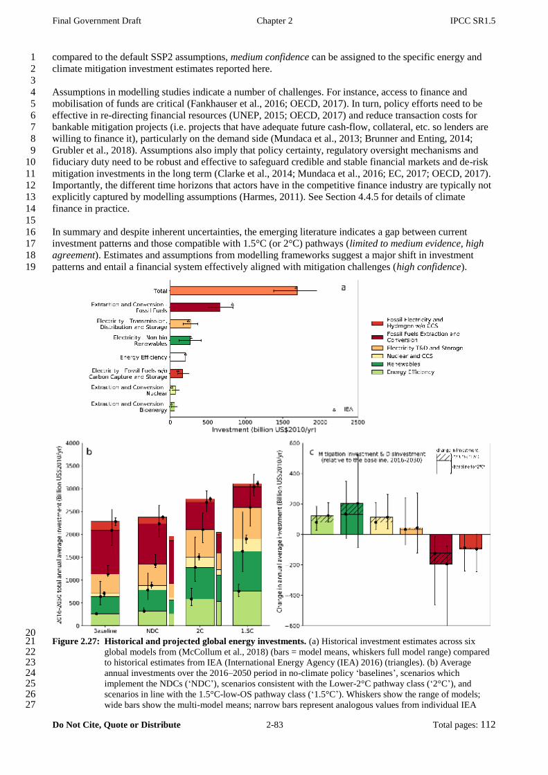
Final Government Draft Chapter 2 IPCC SR1.5
Do Not Cite, Quote or Distribute 2-83 Total pages: 112
compared to the default SSP2 assumptions, medium confidence can be assigned to the specific energy and 1
climate mitigation investment estimates reported here. 2
3
Assumptions in modelling studies indicate a number of challenges. For instance, access to finance and 4
mobilisation of funds are critical (Fankhauser et al., 2016; OECD, 2017). In turn, policy efforts need to be 5
effective in re-directing financial resources (UNEP, 2015; OECD, 2017) and reduce transaction costs for 6
bankable mitigation projects (i.e. projects that have adequate future cash-flow, collateral, etc. so lenders are 7
willing to finance it), particularly on the demand side (Mundaca et al., 2013; Brunner and Enting, 2014; 8
Grubler et al., 2018). Assumptions also imply that policy certainty, regulatory oversight mechanisms and 9
fiduciary duty need to be robust and effective to safeguard credible and stable financial markets and de-risk 10
mitigation investments in the long term (Clarke et al., 2014; Mundaca et al., 2016; EC, 2017; OECD, 2017). 11
Importantly, the different time horizons that actors have in the competitive finance industry are typically not 12
explicitly captured by modelling assumptions (Harmes, 2011). See Section 4.4.5 for details of climate 13
finance in practice. 14
15
In summary and despite inherent uncertainties, the emerging literature indicates a gap between current 16
investment patterns and those compatible with 1.5°C (or 2°C) pathways (limited to medium evidence, high 17
agreement). Estimates and assumptions from modelling frameworks suggest a major shift in investment 18
patterns and entail a financial system effectively aligned with mitigation challenges (high confidence). 19
20 Figure 2.27: Historical and projected global energy investments. (a) Historical investment estimates across six 21
global models from (McCollum et al., 2018) (bars = model means, whiskers full model range) compared 22 to historical estimates from IEA (International Energy Agency (IEA) 2016) (triangles). (b) Average 23 annual investments over the 2016–2050 period in no-climate policy ‘baselines’, scenarios which 24 implement the NDCs (‘NDC’), scenarios consistent with the Lower-2°C pathway class (‘2°C’), and 25 scenarios in line with the 1.5°C-low-OS pathway class (‘1.5°C’). Whiskers show the range of models; 26 wide bars show the multi-model means; narrow bars represent analogous values from individual IEA 27
Final Government Draft Chapter 2 IPCC SR1.5
Do Not Cite, Quote or Distribute 2-84 Total pages: 112
scenarios (OECD/IEA and IRENA, 2017). (c) Average annual mitigation investments and disinvestments 1 for the 2016–2030 periods relative to the baseline. The solid bars show the values for ‘2°C’ pathways, 2 while the hatched areas show the additional investments for the pathways labelled with ‘1.5°C’. Whiskers 3 show the full range around the multi-model means. T&D stands for transmission and distribution, and 4 CCS stands for carbon capture and storage. Global cumulative carbon dioxide emissions, from fossil fuels 5 and industrial processes (FF&I) but excluding land use, over the 2016-2100 timeframe range from 880 to 6 1074 GtCO2 (multi-model mean: 952 GtCO2) in the ‘2°C’ pathway and from 206 to 525 GtCO2 (mean: 7 390 GtCO2) in the ‘1.5°C’ pathway. 8
9
10
2.5.3 Sustainable development features of 1.5°C pathways 11
12
Potential synergies and trade-offs between 1.5°C mitigation pathways and different sustainable development 13
(SD) dimensions (see Cross-Chapter Box 4) are an emerging field of research. Section 5.4 assesses 14
interactions between individual mitigation measures with other societal objectives, as well as the Sustainable 15
Development Goals (SGDs) (Table 5.1). This section synthesized the Chapter 5 insights to assess how these 16
interactions play out in integrated 1.5°C pathways, and the four illustrative pathway archetypes of this 17
chapter in particular (see Section 2.1). Information from integrated pathways is combined with the 18
interactions assessed in Chapter 5 and aggregated for each SDG, with a level of confidence attributed to each 19
interaction based on the amount and agreement of the scientific evidence (see Chapter 5). 20
21
Figure 2.28 shows how the scale and combination of individual mitigation measures (i.e., their mitigation 22
portfolios) influence the extent of synergies and trade-offs with other societal objectives. All pathways 23
generate multiple synergies with SD dimensions and can advance several other SDGs simultaneously. Some, 24
however, show higher risks for trade-offs. An example is increased biomass production and its potential to 25
increase pressure on land and water resources, food production, biodiversity, and reduced air-quality when 26
combusted inefficiently. At the same time, mitigation actions in energy-demand sectors and behavioural 27
response options with appropriate management of rebound effects can advance multiple SDGs 28
simultaneously, more so than energy supply-side mitigation actions (see Section 5.4, Table 5.1 and Figure 29
5.3 for more examples). Of the four pathway archetypes used in this chapter (S1, S2, S5, and LED), the S1 30
and LED pathways show the largest number of synergies and least number of potential trade-offs, while for 31
the S5 pathway most potential trade-offs are identified. In general, pathways with emphasis on demand 32
reductions, with policies that incentivise behavioural change, sustainable consumption patterns, healthy diets 33
and relatively low use of CDR (or only afforestation) show relatively more synergies with individual SDGs 34
than others. 35
36
There is robust evidence and high agreement in the pathway literature that multiple strategies can be 37
considered to limit warming to 1.5°C (see Sections 2.1.3, 2.3 and 2.4). Together with the extensive evidence 38
on the existence of interactions of mitigation measures with other societal objectives (Section 5.4), this 39
results in high confidence that the choice of mitigation portfolio or strategy can markedly affect the 40
achievement of other societal objectives. For instance, action on SLCFs has been suggested to facilitate the 41
achievement of SDGs (Shindell et al., 2017b) and to reduce regional impacts, e.g., from black carbon sources 42
on snow and ice loss in the Arctic and alpine regions (Painter et al., 2013), with particular focus on the 43
warming sub-set of SLCFs. Reductions in both surface aerosols and ozone through methane reductions 44
provide health and ecosystem co-benefits (Jacobson, 2002, 2010; Anenberg et al., 2012; Shindell et al., 45
2012; Stohl et al., 2015; Collins et al., 2018). Public health benefits of stringent mitigation pathways in line 46
with 1.5°C-consistent pathways can be sizeable. For instance, a study examining a more rapid reduction of 47
fossil-fuel usage to achieve 1.5°C relative to 2°C, similar to that of other recent studies (Grubler et al., 2018; 48
van Vuuren et al., 2018), found that improved air quality would lead to more than 100 million avoided 49
premature deaths over the 21st century (Shindell et al., 2018). These benefits are assumed to be in addition to 50
those occurring under 2°C pathways (e.g., Silva et al., 2016), and could in monetary terms offset a large 51
portion to all of the initial mitigation costs (West et al., 2013; Shindell et al., 2018). However, some sources 52
of SLCFs with important impacts for public health (e.g., traditional biomass burning) are only mildly 53
affected by climate policy in the available integrated pathways and are more strongly impacted by baseline 54
assumptions about future societal development and preferences, and technologies instead (Rao et al., 2016, 55
2017). 56
At the same time, the literature on climate-SDG interactions is still an emergent field of research and hence 57
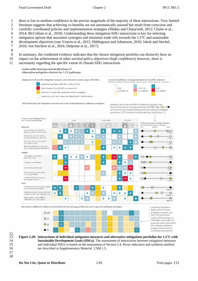
Final Government Draft Chapter 2 IPCC SR1.5
Do Not Cite, Quote or Distribute 2-85 Total pages: 112
there is low to medium confidence in the precise magnitude of the majority of these interactions. Very limited 1
literature suggests that achieving co-benefits are not automatically assured but result from conscious and 2
carefully coordinated policies and implementation strategies (Shukla and Chaturvedi, 2012; Clarke et al., 3
2014; McCollum et al., 2018). Understanding these mitigation-SDG interactions is key for selecting 4
mitigation options that maximise synergies and minimize trade-offs towards the 1.5°C and sustainable 5
development objectives (van Vuuren et al., 2015; Hildingsson and Johansson, 2016; Jakob and Steckel, 6
2016; von Stechow et al., 2016; Delponte et al., 2017). 7
8
In summary, the combined evidence indicates that the chosen mitigation portfolio can distinctly have an 9
impact on the achievement of other societal policy objectives (high confidence); however, there is 10
uncertainty regarding the specific extent of climate-SDG interactions. 11
12 Figure 2.28: Interactions of individual mitigation measures and alternative mitigations portfolios for 1.5°C with 13
Sustainable Development Goals (SDGs). The assessment of interactions between mitigation measures 14 and individual SDGs is based on the assessment of Section 5.4. Proxy indicators and synthesis method 15 are described in Supplementary Material 2.SM.1.5. 16
17 18
Final Government Draft Chapter 2 IPCC SR1.5
Do Not Cite, Quote or Distribute 2-86 Total pages: 112
2.6 Knowledge gaps 1
2
This section summarises the knowledge gaps articulated in earlier sections of the chapter. 3
4
5
2.6.1 Geophysical understanding 6
7
Knowledge gaps are associated with the carbon-cycle response, the role of non-CO2 emissions and on the 8
evaluation of an appropriate historic baseline. 9
10
Quantifying how the carbon cycle responds to negative emissions is an important knowledge gap for strong 11
mitigation pathways (Section 2.2). Earth-system feedback uncertainties are important to consider for the 12
longer-term response, particularly in how permafrost melting might affect the carbon budget (Section 2.2). 13
Future research and ongoing observations over the next years will provide a better indication as to how the 14
2006-2015 base period compares with the long-term trends and might at present bias the carbon budget 15
estimates. 16
17
The future emissions of short-lived climate forcers and their temperature response are a large source of 18
uncertainty in 1.5°C pathways, having a greater relative uncertainty than in higher CO2 emission pathways. 19
Their global emissions, their sectorial and regional disaggregation and their climate response are generally 20
less well quantified than for CO2 (Sections 2.2 and 2.3). Emissions from the agricultural sector including 21
land-use based mitigation options in 1.5°C pathways constitute the main source of uncertainty here and are 22
an important gap in understanding the potential achievement of stringent mitigation scenarios (Sections 2.3 23
and 2.4). This also includes uncertainties surrounding the mitigation potential of the long-lived GHG nitrous 24
oxide. (Sections 2.3 and 2.4) 25
26
There is considerable uncertainty in how future emissions of aerosol precursors will affect the effective 27
radiative forcing from aerosol-cloud interaction. The potential future warming from mitigation of these 28
emissions reduces remaining carbon budgets and increases peak temperatures (Section 2.2). The potential 29
co-benefits of mitigating air pollutants and how the reduction in air pollution may affect the carbon sink are 30
also important sources of uncertainty (Sections 2.2 and 2.5). 31
32
The pathway classification employed in this Chapter employs results from the MAGICC model with its AR5 33
parameter sets. The alternative representation of the relationship between emissions and effective radiative 34
forcing and response in the FAIR model would lead to a different classification that would make 1.5°C 35
targets more achievable (Section 2.2 and Supplementary Material 2.SM.1.1). Such a revision would 36
significantly alter the temperature outcomes for the pathways and, if the result is found to be robust, future 37
research and assessments would need to adjust their classifications accordingly. Any possible high bias in the 38
MAGICC response may be partly or entirely offset by missing Earth system feedbacks that are not 39
represented in either climate emulator that would act to increase the temperature response (Section 2.2). For 40
this assessment report, any possible bias in MAGICC setup applied in this and earlier reports is not 41
established enough in the literature to change the classification approach. However, we only place medium 42
confidence in the classification adopted by the chapter. 43
44
45
2.6.2 Integrated assessment approaches 46
47
IAMs attempt to be as broad as possible in order to explore interactions between various societal subsystems, 48
like the economy, land, and energy system. They hence include stylised and simplified representations of 49
these subsystems. Climate damages, avoided impacts and societal co-benefits of the modelled 50
transformations remain largely unaccounted for and are important knowledge gaps. Furthermore, rapid 51
technological changes and uncertainties about input data present continuous challenges. 52
53
The IAMs used in this report do not account for climate impacts (Section 2.1), and similarly, none of the 54
Gross Domestic Product (GDP) projections in the mitigation pathway literature assessed in this chapter 55
included the feedback of climate damages on economic growth (Section 2.3). Although some IAMs do allow 56
for climate impact feedbacks in their modelling frameworks, particularly in their land components, such 57
Final Government Draft Chapter 2 IPCC SR1.5
Do Not Cite, Quote or Distribute 2-87 Total pages: 112
feedbacks were by design excluded in pathways developed in the context of the SSP framework. The SSP 1
framework aims at providing an integrative framework for the assessment of climate change adaptation and 2
mitigation. IAMs are typically developed to inform the mitigation component of this question, while the 3
assessment of impacts is carried out by specialized impact models. However, the use of a consistent set of 4
socio-economic drivers embodied by the SSPs allows for an integrated assessment of climate change impacts 5
and mitigation challenges at a later stage. Further integration of these two strands of research will allow a 6
better understanding of climate impacts on mitigation studies. 7
8
Many of the IAMs that contributed mitigation pathways to this assessment include a process-based 9
description of the land system in addition to the energy system and several have been extended to cover air 10
pollutants and water use. These features make them increasingly fit to explore questions beyond those that 11
touch upon climate mitigation only. The models do not, however, fully account for all constraints that could 12
affect realization of pathways (Section 2.1). 13
14
While the representation of renewable energy resource potentials, technology costs and system integration in 15
IAMs has been updated since AR5, bottom-up studies find higher mitigation potentials in the industry, 16
buildings, and transport sector in that realized by selected pathways from IAMs, indicating the possibility to 17
strengthen sectorial decarbonisation strategies compared to the IAM 1.5°C pathways assessed in this chapter 18
(Section 2.1). 19
20
Studies indicate that a major shift in investment patterns is required to limit global warming to 1.5°C. This 21
assessment would benefit from a more explicit representation and understanding of the financial sector 22
within the modelling approaches. Assumptions in modelling studies imply low-to-zero transaction costs for 23
market agents and that regulatory oversight mechanisms and fiduciary duty need to be highly robust to 24
guarantee stable and credible financial markets in the long term. This area can be subject to high uncertainty, 25
however. The heterogeneity of actors (e.g., banks, insurance companies, asset managers, or credit rating 26
agencies) and financial products also needs to be taken into account, as does the mobilisation of capital and 27
financial flows between countries and regions (Section 2.5). 28
29
The literature on interactions between 1.5˚C mitigation pathways and SDGs is an emergent field of research 30
(Section 2.3.5, 2.5 and Chapter 5). Whereas the choice of mitigation strategies can noticeably affect the 31
attainment of various societal objectives, there is uncertainty regarding the extent of the majority of 32
identified interactions. Understanding climate-SDG interactions helps the choice of mitigation options that 33
minimize trade-offs and risks and maximise synergies towards sustainable development objectives and the 34
1.5°C goal (Section 2.5). 35
36
37
2.6.3 Carbon Dioxide Removal (CDR) 38
39
Most 1.5°C and 2°C pathways are heavily reliant on CDR at a speculatively large scale before mid-century. 40
There are a number of knowledge gaps associated which such technologies. Chapter 4 performs a detailed 41
assessment of CDR technologies. 42
43
There is uncertainty in the future deployment of CCS given the limited pace of current deployment, the 44
evolution of CCS technology that would be associated with deployment, and the current lack of incentives 45
for large-scale implementation of CCS (Section 4.2.7). Technologies other than BECCS and afforestation 46
have yet to be comprehensively assessed in integrated assessment approaches. No proposed technology is 47
close to deployment at scale and regulatory frameworks are not established. This limits how they can be 48
realistically implemented within IAMs. (Section 2.3) 49
50
Evaluating the potential from BECCS is problematic due to large uncertainties in future land projections due 51
to differences in modelling approaches in current land-use models which are at least as great as the 52
differences attributed to climate scenario variations. (Section 2.3) 53
54
There is substantial uncertainty about the adverse effects of large-scale CDR deployment on the environment 55
and societal sustainable development goals. It is not fully understood how land use and land management 56
choices for large-scale BECCS will affect various ecosystem services and sustainable development, and 57
Final Government Draft Chapter 2 IPCC SR1.5
Do Not Cite, Quote or Distribute 2-88 Total pages: 112
further translate into indirect impacts on climate including GHG emissions other than CO2. (Section 2.3, 1
Section 2.5.3) 2
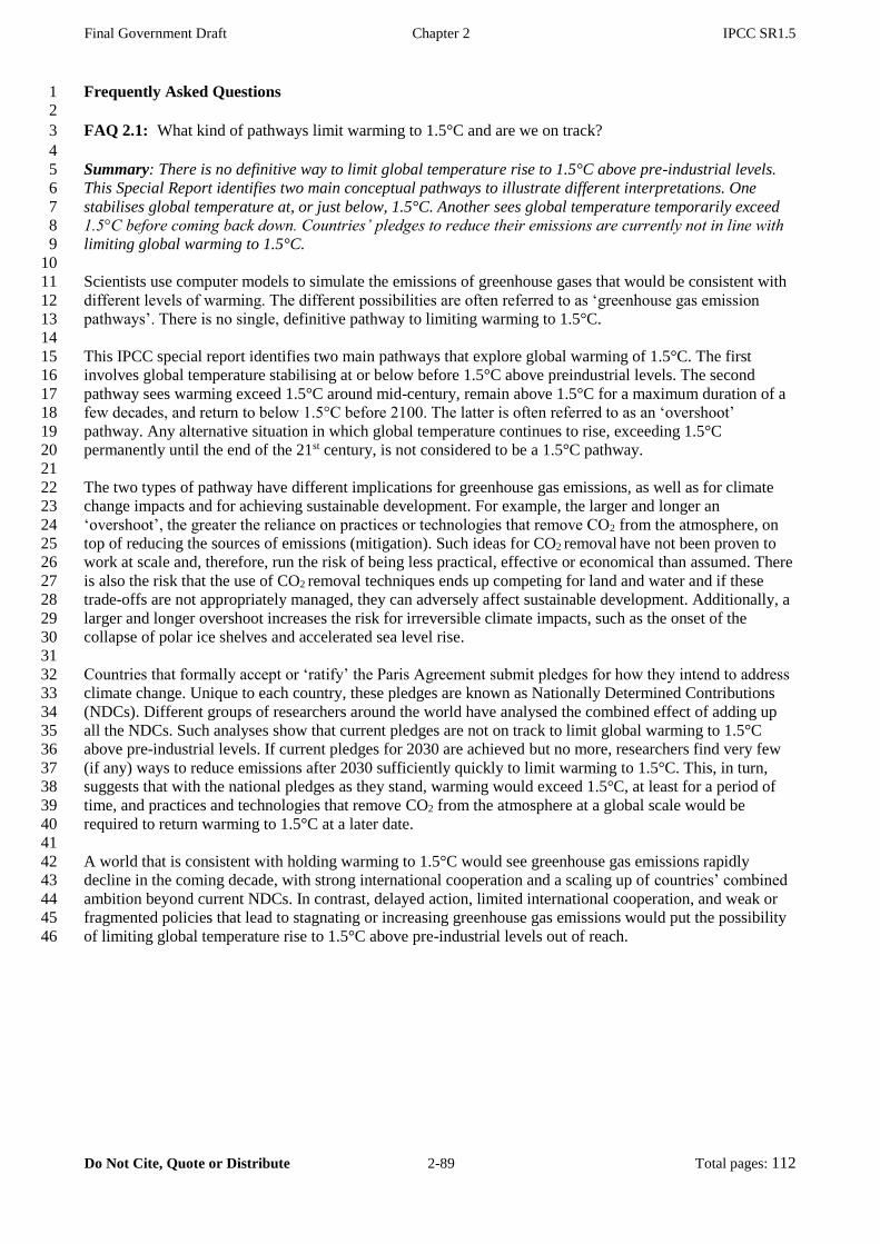
Final Government Draft Chapter 2 IPCC SR1.5
Do Not Cite, Quote or Distribute 2-89 Total pages: 112
Frequently Asked Questions 1 2
FAQ 2.1: What kind of pathways limit warming to 1.5°C and are we on track? 3
4
Summary: There is no definitive way to limit global temperature rise to 1.5°C above pre-industrial levels. 5
This Special Report identifies two main conceptual pathways to illustrate different interpretations. One 6
stabilises global temperature at, or just below, 1.5°C. Another sees global temperature temporarily exceed 7
1.5°C before coming back down. Countries’ pledges to reduce their emissions are currently not in line with 8
limiting global warming to 1.5°C. 9
10
Scientists use computer models to simulate the emissions of greenhouse gases that would be consistent with 11
different levels of warming. The different possibilities are often referred to as ‘greenhouse gas emission 12
pathways’. There is no single, definitive pathway to limiting warming to 1.5°C. 13
14
This IPCC special report identifies two main pathways that explore global warming of 1.5°C. The first 15
involves global temperature stabilising at or below before 1.5°C above preindustrial levels. The second 16
pathway sees warming exceed 1.5°C around mid-century, remain above 1.5°C for a maximum duration of a 17
few decades, and return to below 1.5°C before 2100. The latter is often referred to as an ‘overshoot’ 18
pathway. Any alternative situation in which global temperature continues to rise, exceeding 1.5°C 19
permanently until the end of the 21st century, is not considered to be a 1.5°C pathway. 20
21
The two types of pathway have different implications for greenhouse gas emissions, as well as for climate 22
change impacts and for achieving sustainable development. For example, the larger and longer an 23
‘overshoot’, the greater the reliance on practices or technologies that remove CO2 from the atmosphere, on 24
top of reducing the sources of emissions (mitigation). Such ideas for CO2 removal have not been proven to 25
work at scale and, therefore, run the risk of being less practical, effective or economical than assumed. There 26
is also the risk that the use of CO2 removal techniques ends up competing for land and water and if these 27
trade-offs are not appropriately managed, they can adversely affect sustainable development. Additionally, a 28
larger and longer overshoot increases the risk for irreversible climate impacts, such as the onset of the 29
collapse of polar ice shelves and accelerated sea level rise. 30
31
Countries that formally accept or ‘ratify’ the Paris Agreement submit pledges for how they intend to address 32
climate change. Unique to each country, these pledges are known as Nationally Determined Contributions 33
(NDCs). Different groups of researchers around the world have analysed the combined effect of adding up 34
all the NDCs. Such analyses show that current pledges are not on track to limit global warming to 1.5°C 35
above pre-industrial levels. If current pledges for 2030 are achieved but no more, researchers find very few 36
(if any) ways to reduce emissions after 2030 sufficiently quickly to limit warming to 1.5°C. This, in turn, 37
suggests that with the national pledges as they stand, warming would exceed 1.5°C, at least for a period of 38
time, and practices and technologies that remove CO2 from the atmosphere at a global scale would be 39
required to return warming to 1.5°C at a later date. 40
41
A world that is consistent with holding warming to 1.5°C would see greenhouse gas emissions rapidly 42
decline in the coming decade, with strong international cooperation and a scaling up of countries’ combined 43
ambition beyond current NDCs. In contrast, delayed action, limited international cooperation, and weak or 44
fragmented policies that lead to stagnating or increasing greenhouse gas emissions would put the possibility 45
of limiting global temperature rise to 1.5°C above pre-industrial levels out of reach. 46
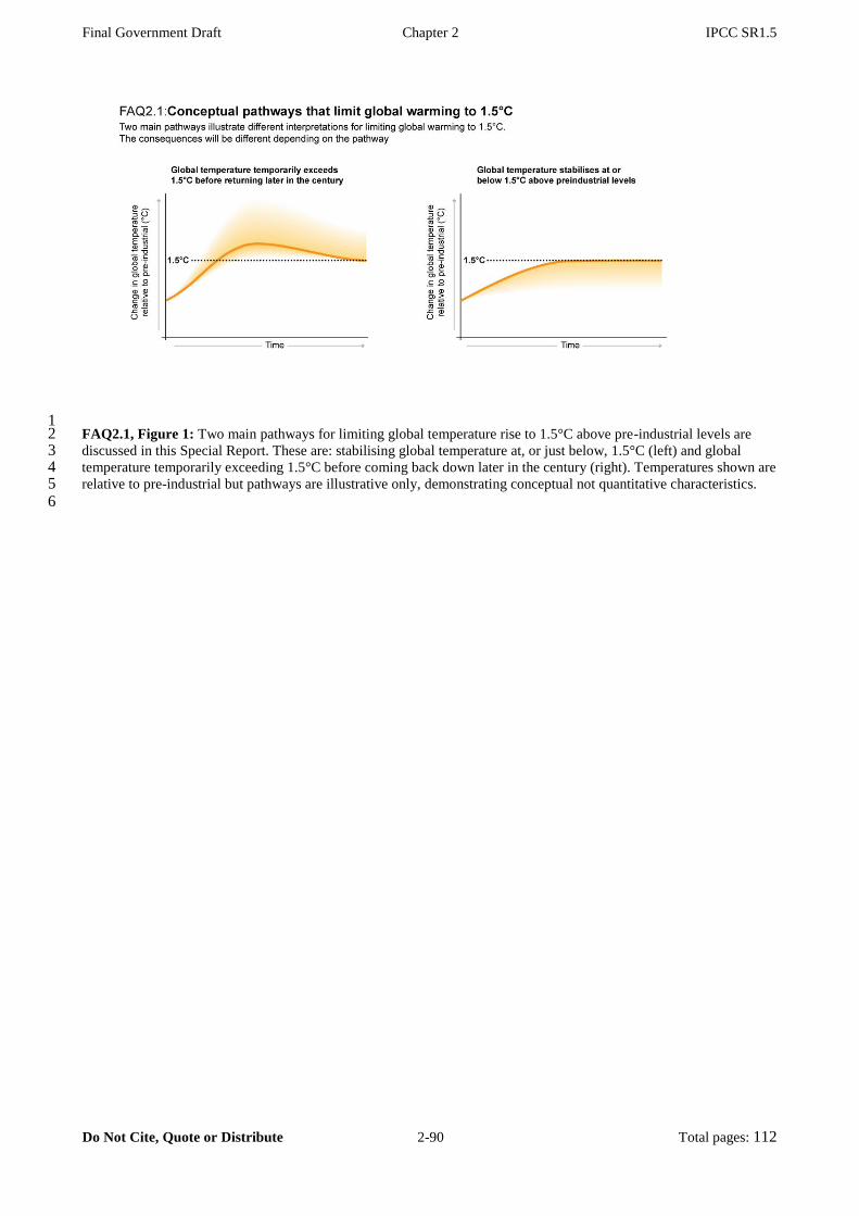
Final Government Draft Chapter 2 IPCC SR1.5
Do Not Cite, Quote or Distribute 2-90 Total pages: 112
1 FAQ2.1, Figure 1: Two main pathways for limiting global temperature rise to 1.5°C above pre-industrial levels are 2 discussed in this Special Report. These are: stabilising global temperature at, or just below, 1.5°C (left) and global 3 temperature temporarily exceeding 1.5°C before coming back down later in the century (right). Temperatures shown are 4 relative to pre-industrial but pathways are illustrative only, demonstrating conceptual not quantitative characteristics. 5 6

Final Government Draft Chapter 2 IPCC SR1.5
Do Not Cite, Quote or Distribute 2-91 Total pages: 112
1
FAQ 2.2: What do energy supply and demand have to do with limiting warming to 1.5°C? 2
3
Summary: Limiting global warming to 1.5°C above pre-industrial levels would require major reductions in 4
greenhouse gas emissions in all sectors. But different sectors are not independent of each other and making 5
changes in one can have implications for another. For example, if we as a society use a lot of energy, then 6
this could mean we have less flexibility in the choice of mitigation options available to limit warming to 7
1.5°C. If we use less energy, the choice of possible actions is greater. For example we could be less reliant 8
on technologies that remove carbon dioxide (CO2) from the atmosphere. 9
10
To stabilise global temperature at any level, ‘net’ CO2 emissions would need to be reduced to zero. This 11
means the amount of CO2 entering the atmosphere must equal the amount that is removed. Achieving a 12
balance between CO2 ‘sources’ and ‘sinks’ is often referred to as ‘net zero’ emissions or ‘carbon neutrality’. 13
The implication of net zero emissions is that the concentration of CO2 in the atmosphere would slowly 14
decline over time until a new equilibrium is reached, as CO2 emissions from human activity are redistributed 15
and taken up by the oceans and the land biosphere. This would lead to a near-constant global temperature 16
over many centuries. 17
18
Warming will not be limited to 1.5°C or 2°C unless transformations in a number of areas achieve the 19
required greenhouse gas emissions reductions. Emissions would need to decline rapidly across all of 20
society’s main sectors, including buildings, industry, transport, energy, and agriculture, forestry and other 21
land use (AFOLU). Actions that can reduce emissions include, for example, phasing out coal in the energy 22
sector, increasing the amount of energy produced from renewable sources, electrifying transport, and 23
reducing the ‘carbon footprint’ of the food we consume. 24
25
The above are examples of ‘supply-side’ actions. Broadly speaking, these are actions that can reduce 26
greenhouse gas emissions through the use of low-carbon solutions. A different type of action can reduce how 27
much energy human society uses, while still ensuring increasing levels of development and well-being. 28
Known as ‘demand-side’ actions, this category includes improving energy efficiency in buildings and 29
reducing consumption of energy- and greenhouse-gas intensive products through behavioural and lifestyle 30
changes, for example. Demand and supply-side measures are not an either-or question, they work in parallel 31
with each other. But emphasis can be given to one or the other. 32
33
Making changes in one sector can have consequences for another, as they are not independent of each other. 34
In other words, the choices that we make now as a society in one sector can either restrict or expand our 35
options later on. For example, a high demand for energy could mean we would need to deploy almost all 36
known options to reduce emissions in order to limit global temperature rise to 1.5°C above pre-industrial 37
levels, with the potential for adverse side-effects. For example, a high-demand pathway increases our 38
reliance on practices and technologies that remove CO2 from the atmosphere. As of yet, such techniques 39
have not been proven to work on a large scale and, depending on how they are implemented, could compete 40
for land and water. By leading to lower overall energy demand, effective demand-side measures could allow 41
for greater flexibility in how we structure our energy system. However, demand-side measures are not easy 42
to implement and barriers have prevented the most efficient practices being used in the past. 43
44
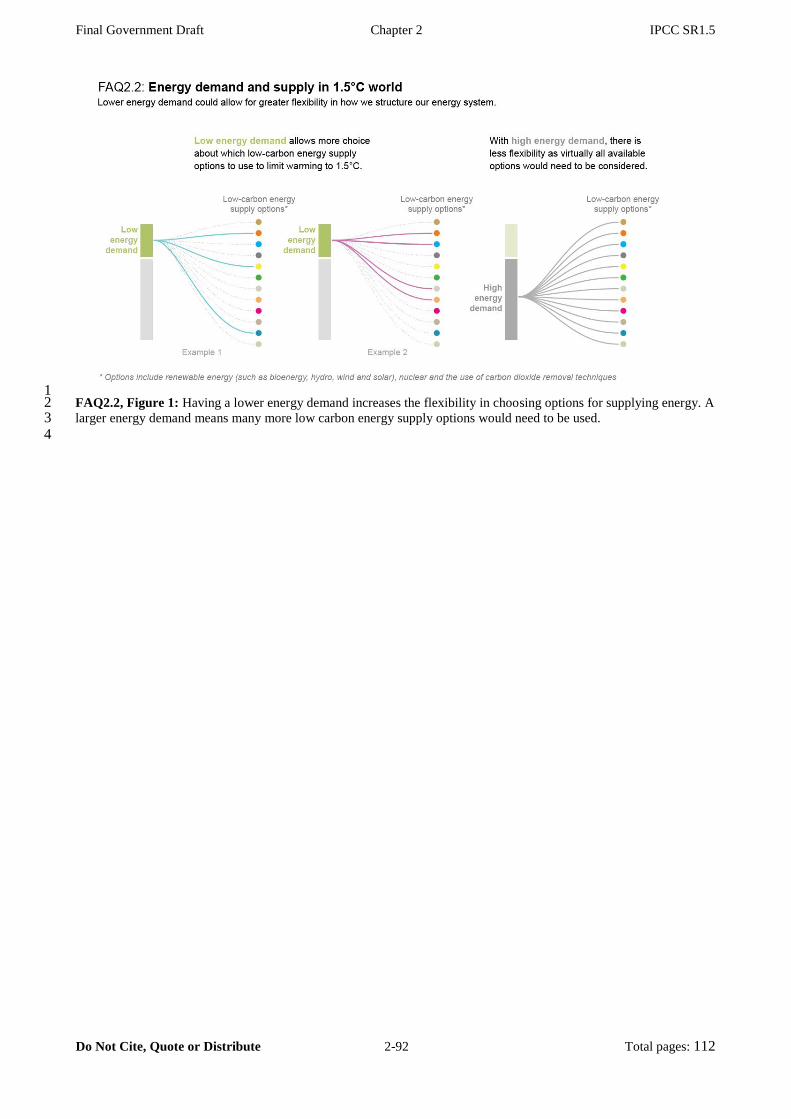
Final Government Draft Chapter 2 IPCC SR1.5
Do Not Cite, Quote or Distribute 2-92 Total pages: 112
1 FAQ2.2, Figure 1: Having a lower energy demand increases the flexibility in choosing options for supplying energy. A 2 larger energy demand means many more low carbon energy supply options would need to be used. 3 4
Final Government Draft Chapter 2 IPCC SR1.5
Do Not Cite, Quote or Distribute 2-93 Total pages: 112
References 1 2 Ackerman, F. and E.A. Stanton, 2012: Climate Risks and Carbon Prices: Revising the Social Cost of Carbon. 3
Economics: The Open-Access, Open-Assessment E-Journal, 6(2012-10), 1, doi:10.5018/economics-4 ejournal.ja.2012-10. 5
Adler, M.D. and N. Treich, 2015: Prioritarianism and Climate Change. Environmental and Resource Economics, 62(2), 6 279-308, doi:10.1007/s10640-015-9960-7. 7
Adler, M.D. et al., 2017: Priority for the worse-off and the social cost of carbon. Nature Clim. Change, 7(6), 443-449, 8 doi:10.1038/nclimate3298. 9
Akimoto, K., F. Sano, and T. Tomoda, 2017: GHG emission pathways until 2300 for the 1.5 °C temperature rise target 10 and the mitigation costs achieving the pathways. Mitigation and Adaptation Strategies for Global Change, 1-11 14, doi:10.1007/s11027-017-9762-z. 12
Alcalde, J. et al., 2018: Estimating geological CO2 storage security to deliver on climate mitigation. Nature 13 Communications (in press), doi:10.1038/s41467-018-04423-1. 14
Aldy, J.E. and R.N. Stavins, 2012: The Promise and Problems of Pricing Carbon. The Journal of Environment & 15 Development, 21(2), 152-180, doi:10.1177/1070496512442508. 16
Aldy, J.E. et al., 2016: Economic tools to promote transparency and comparability in the Paris Agreement. Nature 17 Climate Change, 6(11), 1000-1004, doi:10.1038/nclimate3106. 18
Allen, M.R. et al., 2009: Warming caused by cumulative carbon emissions towards the trillionth tonne. Nature, 19 458(7242), 1163-1166, doi:10.1038/nature08019. 20
Allen, M.R. et al., 2016: New use of global warming potentials to compare cumulative and short-lived climate 21 pollutants. Nature Climate Change, 6(May), 1-5, doi:10.1038/nclimate2998. 22
Allen, M.R. et al., 2018: A solution to the misrepresentations of CO2-equivalent emissions of short-lived climate 23 pollutants under ambitious mitigation. npj Climate and Atmospheric Science (in press). 24
Allwood, J.M., M.F. Ashby, T.G. Gutowski, and E. Worrell, 2013: Material efficiency: providing material services with 25 less material production. Phil. Trans. R. Soc. A, 371(1986), 20120496, doi:10.1098/rsta.2012.0496. 26
Anderson, K. and G. Peters, 2016: The trouble with negative emissions. Science, 354(6309), 182-183, 27 doi:10.1126/science.aah4567. 28
Anenberg, S.C. et al., 2012: Global Air Quality and Health Co-benefits of Mitigating Near-Term Climate Change 29 through Methane and Black Carbon Emission Controls. Environmental Health Perspectives, 120(6), 831-839, 30 doi:10.1289/ehp.1104301. 31
Anthoff, D. and R.S.J. Tol, 2009: The impact of climate change on the balanced growth equivalent: An application of 32 FUND. Environmental and Resource Economics, 43(3), 351-367, doi:10.1007/s10640-009-9269-5. 33
Armour, K.C., 2017: Energy budget constraints on climate sensitivity in light of inconstant climate feedbacks. Nature 34 Clim. Change, 7(5), 331-335, doi:10.1038/nclimate3278. 35
Arneth, A. et al., 2010: Terrestrial biogeochemical feedbacks in the climate system. Nature Geoscience, 3(8), 525-532, 36 doi:10.1038/ngeo905. 37
Arroyo-Currás, T. et al., 2015: Carbon leakage in a fragmented climate regime: The dynamic response of global energy 38 markets. Technological Forecasting & Social Change, 90, 192-203, doi:10.1016/j.techfore.2013.10.002. 39
Bachu, S., 2015: Review of CO2 storage efficiency in deep saline aquifers. International Journal of Greenhouse Gas 40 Control, 40, 188-202, doi:10.1016/j.ijggc.2015.01.007. 41
Bachu, S. et al., 2007a: Phase II Final Report from the Task Force for Review and Identification of Standards for CO2 42 Storage Capacity Estimation. Estimation of CO2 Storage Capacity in Geological Media - Phase 2, 43 pp. 43
Bachu, S. et al., 2007b: CO2 storage capacity estimation: Methodology and gaps. International Journal of Greenhouse 44 Gas Control, 1(4), 430-443, doi:10.1016/S1750-5836(07)00086-2. 45
Bajželj, B. et al., 2014: Importance of food-demand management for climate mitigation. Nature Climate Change, 4(10), 46 924-929, doi:10.1038/nclimate2353. 47
Banerjee, R. et al., 2012: GEA Chapter 8 - Energy End Use: Industry. In: Global Energy Assessment - Toward a 48 Sustainable Future. Cambridge University Press, Cambridge, UK and New York, NY, USA and the 49 International Institute for Applied Systems Analysis, Laxenburg, Austria, pp. 513-574. 50
Baranzini, A. et al., 2017: Carbon pricing in climate policy: seven reasons, complementary instruments, and political 51 economy considerations. Wiley Interdisciplinary Reviews: Climate Change, 8(4), e462, doi:10.1002/wcc.462. 52
Bataille, C., H. Waisman, M. Colombier, L. Segafredo, and J. Williams, 2016a: The Deep Decarbonization Pathways 53 Project (DDPP): insights and emerging issues. Climate Policy, 16(sup1), S1-S6, 54 doi:10.1080/14693062.2016.1179620. 55
Bataille, C. et al., 2016b: The need for national deep decarbonization pathways for effective climate policy. Climate 56 Policy, 16(sup1), S7-S26, doi:10.1080/14693062.2016.1173005. 57
Bauer, N. et al., 2017: Shared Socio-Economic Pathways of the Energy Sector - Quantifying the Narratives. Global 58 Environmental Change, 42, 316-330, doi:10.1016/j.gloenvcha.2016.07.006. 59
Bauer, N. et al., 2018: Global energy sector emission reductions and bioenergy use: overview of the bioenergy demand 60 phase of the EMF 33 model comparison. Climatic Change (in press), doi:10.1007/s10584-018-2226-y. 61
Beck, S. and M. Mahony, 2017: The IPCC and the politics of anticipation. Nature Climate Change, 7(5), 311-313, 62
Final Government Draft Chapter 2 IPCC SR1.5
Do Not Cite, Quote or Distribute 2-94 Total pages: 112
doi:10.1038/nclimate3264. 1 Bentham, M., T. Mallows, J. Lowndes, and A. Green, 2014: CO2 STORage evaluation database (CO2 Stored). The UK's 2
online storage atlas. Energy Procedia, 63, 5103-5113, doi:10.1016/j.egypro.2014.11.540. 3 Benveniste, H. et al., 2018: Impacts of nationally determined contributions on 2030 global greenhouse gas emissions: 4
Uncertainty analysis and distribution of emissions. Environmental Research Letters, 13(1), 014022, 5 doi:10.1088/1748-9326/aaa0b9. 6
Berger, A. et al., 2017a: Nuclear energy and bio energy carbon capture and storage, keys for obtaining 1.5°C mean 7 surface temperature limit. International Journal of Global Energy Issues, 40(3/4), 240, 8 doi:10.1504/IJGEI.2017.086622. 9
Berger, A. et al., 2017b: How much can nuclear energy do about global warming? International Journal of Global 10 Energy Issues, 40(1/2), 43, doi:10.1504/IJGEI.2017.080766. 11
Bertram, C., G. Luderer, A. Popp, J.C. Minx, and W. Lamb, 2018: Targeted policies can compensate most of the 12 increased sustainability risks in 1.5°C mitigation scenarios. Environ. Res. Lett (in press), doi: 10.1088/1748-13 9326/aac3ec. 14
Bertram, C. et al., 2015a: Carbon lock-in through capital stock inertia associated with weak near-term climate policies. 15 Technological Forecasting and Social Change, 90(PA), 62-72, doi:10.1016/j.techfore.2013.10.001. 16
Bertram, C. et al., 2015b: Complementing carbon prices with technology policies to keep climate targets within reach. 17 Nature Climate Change, 5(3), 235-239, doi:10.1038/nclimate2514. 18
Bindoff, N. et al., 2013: Detection and Attribution of Climate Change: from Global to Regional. In: Climate Change 19 2013: The Physical Science Basis. Contribution of Working Group I to the Fifth Assessment Report of the 20 Intergovernmental Panel on Climate Change [Stocker, T.F., D. Qin, G.K. Plattner, M. Tignor, S.K. Allen, J. 21 Boschung, A. Nauels, Y. Xia, V. Bex, and P.M. Midgley (eds.)]. Cambridge University Press, Cambridge, 22 United Kingdom and New York, NY, USA, pp. 867-952. 23
Blanco, G. et al., 2014: Drivers, Trends and Mitigation. In: Climate Change 2014: Mitigation of Climate Change. 24 Contribution of Working Group III to the Fifth Assessment Report of the Intergovernmental Panel on Climate 25 Change [Edenhofer, O., R. Pichs-Madruga, Y. Sokona, E. Farahani, S. Kadner, K. Seyboth, A. Adler, I. Baum, 26 S. Brunner, P. Eickemeier, B. Kriemann, J. Savolainen, S. Schlömer, C. von Stechow, T. Zwickel, and J.C. 27 Minx (eds.)]. Cambridge University Press, Cambridge, United Kingdom and New York, NY, USA, pp. 351-28 412. 29
Boardman, A.E., 2006: Cost-Benefit Analysis: Concepts and Practice. Pearson/Prentice Hall, 560 pp. 30 Bodirsky, B.L. et al., 2012: N2O emissions from the global agricultural nitrogen cycle-current state and future 31
scenarios. Biogeosciences, 9(10), 4169-4197, doi:10.5194/bg-9-4169-2012. 32 Bodirsky, B.L. et al., 2014: Reactive nitrogen requirements to feed the world in 2050 and potential to mitigate nitrogen 33
pollution. Nature Communications, 5, doi:10.1038/ncomms4858. 34 Bond, T.C. et al., 2013: Bounding the role of black carbon in the climate system: A scientific assessment. Journal of 35
Geophysical Research: Atmospheres, 118(11), 5380-5552, doi:10.1002/jgrd.50171. 36 Bonsch, M. et al., 2014: Trade-offs between land and water requirements for large-scale bioenergy production. GCB 37
Bioenergy, 8(1), 11-24, doi:10.1111/gcbb.12226. 38 Bosetti, V. and D.G. Victor, 2011: Politics and Economics of Second-Best Regulation of Greenhouse Gases: The 39
Importance of Regulatory Credibility. The Energy Journal, 32(1), 1-24. 40 Bosetti, V., C. Carraro, E. Massetti, and M. Tavoni, 2008: International energy R&D spillovers and the economics of 41
greenhouse gas atmospheric stabilization. Energy Economics, 30(6), 2912-2929, 42 doi:10.1016/j.eneco.2008.04.008. 43
Bosetti, V., C. Carraro, A. Sgobbi, and M. Tavoni, 2009: Delayed action and uncertain stabilisation targets. How much 44 will the delay cost? Climatic Change, 96(3), 299-312, doi:10.1007/s10584-009-9630-2. 45
Bosetti, V., C. Carraro, M. Galeotti, E. Massetti, and M. Tavoni, 2006: WITCH - A world induced technical change 46 hybrid model. The Energy Journal, Special Issue. Hybrid Modeling of Energy-Environment Policies: 47 Reconciling Bottom-up and Top-down, 13-38. 48
Bosetti, V. et al., 2015: Sensitivity to energy technology costs: A multi-model comparison analysis. Energy Policy, 80, 49 244-263, doi:10.1016/j.enpol.2014.12.012. 50
Boucher, O. and G.A. Folberth, 2010: New Directions: Atmospheric methane removal as a way to mitigate climate 51 change? Atmospheric Environment, 44(27), 3343-3345, doi:10.1016/J.ATMOSENV.2010.04.032. 52
Bowen, A., E. Campiglio, and M. Tavoni, 2014: A macroeconomic perspective on climate change mitigation: Meeting 53 the financing challenge. Climate Change Economics, 05(01), 1440005, doi:10.1142/S2010007814400053. 54
Bowerman, N.H.A., D.J. Frame, C. Huntingford, J.A. Lowe, and M.R. Allen, 2011: Cumulative carbon emissions, 55 emissions floors and short-term rates of warming: implications for policy. Philosophical Transactions of the 56 Royal Society A: Mathematical, Physical and Engineering Sciences, 369(1934), 45-66, 57 doi:10.1098/rsta.2010.0288. 58
Bowerman, N.H.A. et al., 2013: The role of short-lived climate pollutants in meeting temperature goals. Nature Climate 59 Change, 3(12), 1021-1024, doi:10.1038/nclimate2034. 60
Boysen, L.R., W. Lucht, and D. Gerten, 2017a: Trade-offs for food production, nature conservation and climate limit 61 the terrestrial carbon dioxide removal potential. Global Change Biology, 23(10), 4303-4317, 62 doi:doi:10.1111/gcb.13745. 63

Final Government Draft Chapter 2 IPCC SR1.5
Do Not Cite, Quote or Distribute 2-95 Total pages: 112
Boysen, L.R., W. Lucht, D. Gerten, and V. Heck, 2016: Impacts devalue the potential of large-scale terrestrial CO2 1 removal through biomass plantations. Environmental Research Letters, 11(9), 1-10, doi:10.1088/1748-2 9326/11/9/095010. 3
Boysen, L.R. et al., 2017b: The limits to global-warming mitigation by terrestrial carbon removal. Earth's Future, 5(5), 4 463-474, doi:10.1002/2016EF000469. 5
Breyer, C. et al., 2017: On the role of solar photovoltaics in global energy transition scenarios. Progress in 6 Photovoltaics: Research and Applications, 25(8), 727-745, doi:10.1002/pip.2885. 7
Brown, M.A. and Y. Li, 2018: Carbon Pricing and Energy Efficiency: Pathways to Deep Decarbonization of the U.S. 8 Electric Sector. Energy Efficiency (in press), doi:10.1007/s12053-018-9686-9. 9
Brown, P.T. and K. Caldeira, 2017: Greater future global warming inferred from Earth's recent energy budget. Nature, 10 552(7683), 45-50, doi:10.1038/nature24672. 11
Bruckner, T., I.A. Bashmakov, and Y. Mulugetta, 2014: Energy Systems. Climate Change 2014: Mitigation of Climate 12 Change. Contribution of Working Group III to the Fifth Assessment Report of the Intergovernmental Panel on 13 Climate Change, 511-598. 14
Brunner, S. and K. Enting, 2014: Climate finance: A transaction cost perspective on the structure of state-to-state 15 transfers. Global Environmental Change, 27, 138-143. 16
Brynolf, S., M. Taljegard, M. Grahn, and J. Hansson, 2018: Electrofuels for the transport sector: A review of production 17 costs. Renewable and Sustainable Energy Reviews, 81, 1887-1905, 18 doi:https://doi.org/10.1016/j.rser.2017.05.288. 19
Buck, H.J., 2016: Rapid scale-up of negative emissions technologies: social barriers and social implications. Climatic 20 Change, 1-13, doi:10.1007/s10584-016-1770-6. 21
Burke, E.J., I.P. Hartley, and C.D. Jones, 2012: Uncertainties in the global temperature change caused by carbon release 22 from permafrost thawing. Cryosphere, 6(5), 1063-1076, doi:10.5194/tc-6-1063-2012. 23
Burke, E.J. et al., 2017: Quantifying uncertainties of permafrost carbon-climate feedbacks. Biogeosciences, 14(12), 24 3051-3066, doi:10.5194/bg-14-3051-2017. 25
Burns, W. and S. Nicholson, 2017: Bioenergy and carbon capture with storage (BECCS): the prospects and challenges 26 of an emerging climate policy response. Journal of Environmental Studies and Sciences, 7(4), 527-534, 27 doi:10.1007/s13412-017-0445-6. 28
Cadule, P., L. Bopp, and P. Friedlingstein, 2009: A revised estimate of the processes contributing to global warming 29 due to climate-carbon feedback. Geophysical Research Letters, 36(14), doi:10.1029/2009GL038681. 30
Cai, Y., K.L. Judd, T.M. Lenton, T.S. Lontzek, and D. Narita, 2015: Environmental tipping points significantly affect 31 the cost-benefit assessment of climate policies. Proceedings of the National Academy of Sciences, 112(15), 32 4606-4611, doi:10.1073/pnas.1503890112. 33
Calvin, K. et al., 2014: Trade-offs of different land and bioenergy policies on the path to achieving climate targets. 34 Climatic Change, 123(3-4), 691-704, doi:10.1007/s10584-013-0897-y. 35
Calvin, K. et al., 2017: The SSP4: A world of deepening inequality. Global Environmental Change, 42, 284-296, 36 doi:10.1016/j.gloenvcha.2016.06.010. 37
Canadell, J.G. and M.R. Raupach, 2008: Managing Forests for Climate Change Mitigation. Science, 320(5882), 1456-38 1457, doi:10.1126/SCIENCE.1155458. 39
Carslaw, K.S. et al., 2013: Large contribution of natural aerosols to uncertainty in indirect forcing. Nature, 503(7474), 40 doi:10.1038/nature12674. 41
Ceppi, P. and J.M. Gregory, 2017: Relationship of tropospheric stability to climate sensitivity and Earth's observed 42 radiation budget. Proceedings of the National Academy of Sciences of the United States of America, 43 201714308, doi:10.1073/pnas.1714308114. 44
Chan, S., P. Ellinger, and O. Widerberg, 2018: Exploring national and regional orchestration of non-state action for a < 45 1.5 °C world. International Environmental Agreements: Politics, Law and Economics, 18(1), 135-152, 46 doi:10.1007/s10784-018-9384-2. 47
Chen, C. and M. Tavoni, 2013: Direct air capture of CO2 and climate stabilization: A model based assessment. Climatic 48 Change, 118(1), 59-72, doi:10.1007/s10584-013-0714-7. 49
Choi, Y.S., D. Young, S. Nešić, and L.G.S. Gray, 2013: Wellbore integrity and corrosion of carbon steel in CO2 50 geologic storage environments: A literature review. International Journal of Greenhouse Gas Control, 16, S70 51 - S77, doi:https://doi.org/10.1016/j.ijggc.2012.12.028. 52
Clack, C.T.M. et al., 2017: Evaluation of a proposal for reliable low-cost grid power with 100% wind, water, and solar.. 53 Proceedings of the National Academy of Sciences of the United States of America, 114(26), 6722-6727, 54 doi:10.1073/pnas.1610381114. 55
Clarke, L. et al., 2014: Assessing transformation pathways. In: Climate Change 2014: Mitigation of Climate Change. 56 Contribution of Working Group III to the Fifth Assessment Report of the Intergovernmental Panel on Climate 57 Change [Edenhofer, O., R. Pichs-Madruga, Y. Sokona, E. Farahani, S. Kadner, K. Seyboth, A. Adler, I. Baum, 58 S. Brunner, P. Eickemeier, B. Kriemann, J. Savolainen, S. Schlömer, C. von Stechow, T. Zwickel, and J.C. 59 Minx (eds.)]. Cambridge University Press, Cambridge, United Kingdom and New York, NY, USA, pp. 413-60 510. 61
Collins, M. et al., 2013: Long-term Climate Change: Projections, Commitments and Irreversibility. In: Climate Change 62 2013: The Physical Science Basis. Contribution of Working Group I to the Fifth Assessment Report of the 63

Final Government Draft Chapter 2 IPCC SR1.5
Do Not Cite, Quote or Distribute 2-96 Total pages: 112
Intergovernmental Panel on Climate Change [Stocker, T.F., D. Qin, G.K. Plattner, M. Tignor, S.K. Allen, J. 1 Boschung, A. Nauels, Y. Xia, V. Bex, and P.M. Midgley (eds.)]. Cambridge University Press, Cambridge, 2 United Kingdom and New York, NY, USA, pp. 1029-1136. 3
Collins, W.J. et al., 2018: Increased importance of methane reduction for a 1.5 degree target. Environmental Research 4 Letters, 13(5), 054003, doi:10.1088/1748-9326/aab89c. 5
Comyn-Platt, E. et al., 2018: Natural CH4 release and permafrost thaw lower CO2 emissions to achieve 1.5 and 2°C 6 targets. Nat. Geosci. (in press). 7
Cox, P.M., C. Huntingford, and M.S. Williamson, 2018: Emergent constraint on equilibrium climate sensitivity from 8 global temperature variability. Nature, 553(7688), 319-322, doi:10.1038/nature25450. 9
Crespo Cuaresma, J., 2017: Income projections for climate change research: A framework based on human capital 10 dynamics. Global Environmental Change, 42, 226-236, doi:10.1016/j.gloenvcha.2015.02.012. 11
Creutzig, F., 2016: Evolving Narratives of Low-Carbon Futures in Transportation. Transport Reviews, 36(3), 341-360, 12 doi:10.1080/01441647.2015.1079277. 13
Creutzig, F. et al., 2012: Reconciling top-down and bottom-up modelling on future bioenergy deployment. Nature 14 Climate Change, 2(5), 320-327, doi:10.1038/nclimate1416. 15
Creutzig, F. et al., 2015: Bioenergy and climate change mitigation: an assessment. GCB Bioenergy, 7(5), 916-944, 16 doi:10.1111/gcbb.12205. 17
Creutzig, F. et al., 2017: The underestimated potential of solar energy to mitigate climate change. Nature Energy, 2(9), 18 17140, doi:10.1038/nenergy.2017.140. 19
Davis, S.C. et al., 2013: Management swing potential for bioenergy crops. GCB Bioenergy, 5(6), 623-638, 20 doi:10.1111/gcbb.12042. 21
Davis, S.J. and K. Caldeira, 2010: Consumption-based accounting of CO2 emissions. Proceedings of the National 22 Academy of Sciences of the United States of America, 107(12), 5687-92, doi:10.1073/pnas.0906974107. 23
de Richter, R., T. Ming, P. Davies, W. Liu, and S. Caillol, 2017: Removal of non-CO2 greenhouse gases by large-scale 24 atmospheric solar photocatalysis. Progress in Energy and Combustion Science, 60, 68-96, 25 doi:10.1016/j.pecs.2017.01.001. 26
de Vries, W., M. Posch, D. Simpson, and G.J. Reinds, 2017: Modelling long-term impacts of changes in climate, 27 nitrogen deposition and ozone exposure on carbon sequestration of European forest ecosystems. Science of the 28 Total Environment, 605-606, 1097-1116, doi:10.1016/j.scitotenv.2017.06.132. 29
Dell, M., B.F. Jones, and B.A. Olken, 2014: What Do We Learn from the Weather ? The New Climate-Economy 30 Literature. Journal of Economic Literature, 52(3), 740-798. 31
Dellink, R., J. Chateau, E. Lanzi, and B. Magné, 2017: Long-term economic growth projections in the Shared 32 Socioeconomic Pathways. Global Environmental Change, 42, 1-15, doi:10.1016/j.gloenvcha.2015.06.004. 33
Delponte, I., I. Pittaluga, and C. Schenone, 2017: Monitoring and evaluation of Sustainable Energy Action Plan: 34 Practice and perspective. Energy Policy, 100, 9-17, doi:10.1016/j.enpol.2016.10.003. 35
den Elzen, M.G.J., D.P. van Vuuren, and J. van Vliet, 2010: Postponing emission reductions from 2020 to 2030 36 increases climate risks and long-term costs. Climatic Change, 99(1), 313-320, doi:10.1007/s10584-010-9798-37 5. 38
den Elzen, M.G.J. et al., 2016: Contribution of the G20 economies to the global impact of the Paris agreement climate 39 proposals. Climatic Change, 137(3-4), 655-665, doi:10.1007/s10584-016-1700-7. 40
Dennig, F., M.B. Budolfson, M. Fleurbaey, A. Siebert, and R.H. Socolow, 2015: Inequality, climate impacts on the 41 future poor, and carbon prices. Proceedings of the National Academy of Sciences, 112(52), 15827-15832, 42 doi:10.1073/pnas.1513967112. 43
DOE/NETL, 2013: Cost and performance of PC and IGCC plants for a range of carbon dioxide capture: revision 1. 44 DOE/NETL-2011/1498, National Energy Technology Laboratory (NETL), 518 pp. 45
Doelman, J.C. et al., 2018: Exploring SSP land-use dynamics using the IMAGE model: Regional and gridded scenarios 46 of land-use change and land-based climate change mitigation. Global Environmental Change, 48, 119-135, 47 doi:https://doi.org/10.1016/j.gloenvcha.2017.11.014. 48
Dooley, J.J., 2013: Estimating the supply and demand for deep geologic CO2 storage capacity over the course of the 49 21st century: A meta-analysis of the literature. Energy Procedia, 37, 5141-5150, 50 doi:10.1016/j.egypro.2013.06.429. 51
Dooley, K. and S. Kartha, 2018: Land-based negative emissions: risks for climate mitigation and impacts on sustainable 52 development. International Environmental Agreements: Politics, Law and Economics, 18(1), 79-98, 53 doi:10.1007/s10784-017-9382-9. 54
Duce, R.A. et al., 2008: Impacts of Atmospheric Anthropogenic Nitrogen on the Open Ocean. Science, 320(5878), 893-55 897. 56
EC, 2017: High-Level Expert Group on Sustainable Finance interim report - Financing a sustainable European 57 economy. European Commission, Brussels, Belgium, 72 pp. 58
Edenhofer, O., J.C. Steckel, M. Jakob, and C. Bertram, 2018: Reports of coal's terminal decline may be exaggerated. 59 Environ. Res. Lett, 13, 024019. 60
Erb, K.H., H. Haberl, and C. Plutzar, 2012: Dependency of global primary bioenergy crop potentials in 2050 on food 61 systems, yields, biodiversity conservation and political stability. Energy Policy, 47, 260-269, 62 doi:10.1016/j.enpol.2012.04.066. 63
Final Government Draft Chapter 2 IPCC SR1.5
Do Not Cite, Quote or Distribute 2-97 Total pages: 112
Erb, K.H. et al., 2016a: Biomass turnover time in terrestrial ecosystems halved by land use. Nature Geoscience, 9(9), 1 674-678, doi:10.1038/ngeo2782. 2
Erb, K.H. et al., 2016b: Exploring the biophysical option space for feeding the world without deforestation. Nature 3 Communications, 7, 11382, doi:10.1038/ncomms11382. 4
Erb, K.H. et al., 2018: Unexpectedly large impact of forest management and grazing on global vegetation biomass. 5 Nature, 553, 73-76. 6
Erickson, P., S. Kartha, M. Lazarus, and K. Tempest, 2015: Assessing carbon lock-in. Environmental Research Letters, 7 10(8), 84023. 8
Etminan, M., G. Myhre, E.J. Highwood, and K.P. Shine, 2016: Radiative forcing of carbon dioxide, methane, and 9 nitrous oxide: A significant revision of the methane radiative forcing. Geophysical Research Letters, 43(24), 10 12,614-12,623, doi:10.1002/2016GL071930. 11
Faehn, T. and E. Isaksen, 2016: Diffusion of Climate Technologies in the Presence of Commitment Problems. The 12 Energy Journal, 37(2), 155-180, doi:10.5547/01956574.37.2.tfae. 13
Fankhauser, S., A. Sahni, A. Savvas, and J. Ward, 2016: Where are the gaps in climate finance? Climate and 14 Development, 8(3), 203-206, doi:10.1080/17565529.2015.1064811. 15
FAOSTAT, 2017: Database Collection of the Food and Agriculture Organization of the United Nations. 16 http://www.fao.org/faostat 17
Fawcett, A.A. et al., 2015: Can Paris pledges avert severe climate change? Science, 350(6265), 1168-1169, 18 doi:10.1126/science.aad5761. 19
Forster, P.M., 2016: Inference of Climate Sensitivity from Analysis of Earth's Energy Budget. Annual Review of Earth 20 and Planetary Sciences, 44(1), 85-106, doi:10.1146/annurev-earth-060614-105156. 21
Frank, S. et al., 2017: Reducing greenhouse gas emissions in agriculture without compromising food security? 22 Environmental Research Letters, 12(10), 105004, doi:10.1088/1748-9326/aa8c83. 23
Frank, S. et al., 2018: Structural change as a key component for agricultural non-CO2 mitigation efforts. Nature 24 Communications, 9(1), 1060, doi:10.1038/s41467-018-03489-1. 25
Frankfurt School-UNEP Centre/BNEF, 2017: Global Trends in Renewable Energy Investment 2017. , 90. 26 Fricko, O. et al., 2016: Energy sector water use implications of a 2 °C climate policy. Environmental Research Letters, 27
11(3), 034011, doi:10.1088/1748-9326/11/3/034011. 28 Fricko, O. et al., 2017: The marker quantification of the Shared Socioeconomic Pathway 2: A middle-of-the-road 29
scenario for the 21st century. Global Environmental Change, 42, 251-267, 30 doi:10.1016/j.gloenvcha.2016.06.004. 31
Friedlingstein, P. et al., 2014a: Persistent growth of CO2 emissions and implications for reaching climate targets. Nature 32 Geoscience, 7(10), 709-715, doi:10.1038/ngeo2248. 33
Friedlingstein, P. et al., 2014b: Uncertainties in CMIP5 climate projections due to carbon cycle feedbacks. Journal of 34 Climate, 27(2), 511-526, doi:10.1175/JCLI-D-12-00579.1. 35
Frölicher, T.L. and F. Joos, 2010: Reversible and irreversible impacts of greenhouse gas emissions in multi-century 36 projections with the NCAR global coupled carbon cycle-climate model. Climate Dynamics, 35(7), 1439-1459, 37 doi:10.1007/s00382-009-0727-0. 38
Fuglestvedt, J.S. et al., 2010: Transport impacts on atmosphere and climate: Metrics. Atmospheric Environment, 44(37), 39 4648-4677, doi:10.1016/j.atmosenv.2009.04.044. 40
Fujimori, S., 2017: SSP3: AIM Implementation of Shared Socioeconomic Pathways. Global Environmental Change, 41 42, 268-283, doi:10.1016/j.gloenvcha.2016.06.009. 42
Fujimori, S. et al., 2016: Implication of Paris Agreement in the context of long-term climate mitigation goals. 43 SpringerPlus, 5(1), 1620, doi:10.1186/s40064-016-3235-9. 44
Fuss, S. et al., 2014: Betting on negative emissions. Nature Climate Change, 4(10), 850-853, 45 doi:10.1038/nclimate2392. 46
Fuss, S. et al., 2016: Research priorities for negative emissions. Environmental Research Letters, 11(11), 47 doi:10.1088/1748-9326/11/11/115007. 48
Fuss, S. et al., 2018: Negative emissions - Part 2: Costs, potentials and side effects. Environmental Research Reviews 49 (in press), doi:10.1088/1748-9326/aabf9f. 50
Geden, O., 2015: Policy: Climate advisers must maintain integrity. Nature, 521(7550), 27-28, doi:10.1038/521027a. 51 Geels, F.W., B.K. Sovacool, T. Schwanen, and S. Sorrell, 2017: Sociotechnical transitions for deep decarbonization. 52
Science, 357(6357). 53 Gerber, P.J. et al., 2013: Tackling Climate Change through Livestock: A global assessment of emissions and mitigation 54
opportunities. 115 pp. 55 Gernaat, D.E.H.J. et al., 2015: Understanding the contribution of non-carbon dioxide gases in deep mitigation scenarios. 56
Global Environmental Change, 33, 142-153, doi:10.1016/j.gloenvcha.2015.04.010. 57 Ghan, S.J. et al., 2013: A simple model of global aerosol indirect effects. Journal of Geophysical Research: 58
Atmospheres, 118(12), 6688-6707, doi:10.1002/jgrd.50567. 59 Ghota, S., C. Huizenga, K. Peet, N. Medimorec, and S. Bakker, 2018: Decarbonising Transport to Achieve Paris 60
Agreement Targets. Energy Efficiency (in press). 61 Giannakidis, G., K. Karlsson, M. Labriet, and B. Ó Gallachóir (eds.), 2018: Limiting Global Warming to Well Below 2 62
°C: Energy System Modelling and Policy Development. Springer International Publishing, 423 pp. 63
Final Government Draft Chapter 2 IPCC SR1.5
Do Not Cite, Quote or Distribute 2-98 Total pages: 112
Gillett, N.P., V.K. Arora, D. Matthews, and M.R. Allen, 2013: Constraining the Ratio of Global Warming to 1 Cumulative CO2 Emissions Using CMIP5 Simulations. Journal of Climate, 26(18), 6844-6858, 2 doi:10.1175/JCLI-D-12-00476.1. 3
Gillett, N.P., V.K. Arora, K. Zickfeld, S.J. Marshall, and W.J. Merryfield, 2011: Ongoing climate change following a 4 complete cessation of carbon dioxide emissions. Nature Geoscience, 4(2), 83-87, doi:10.1038/ngeo1047. 5
Global CCS Institute, 2016: The Global Status of CCS: 2016 Summary Report. 28 pp. 6 González-Eguino, M., A. Olabe, and T. Ribera, 2017: New Coal-Fired Plants Jeopardise Paris Agreement. 7
Sustainability, 9(2). 8 Goodwin, P., S. Brown, I.D. Haigh, R.J. Nicholls, and J.M. Matter, 2018a: Adjusting Mitigation Pathways to Stabilize 9
Climate at 1.5°C and 2.0°C Rise in Global Temperatures to Year 2300. Earth's Future, 0-3, 10 doi:10.1002/2017EF000732. 11
Goodwin, P. et al., 2018b: Pathways to 1.5 and 2 °C warming based on observational and geological constraints. Nature 12 Geoscience, 11(1), 1-22, doi:10.1038/s41561-017-0054-8. 13
Gough, C. and P. Upham, 2011: Biomass energy with carbon capture and storage (BECCS or Bio-CCS). Greenhouse 14 Gases: Science and Technology, 1(4), 324-334, doi:10.1002/ghg.34. 15
Goulder, L. and A. Schein, 2013: Carbon Taxes vs. Cap and Trade: A Critical Review. Climate Change Economics, 16 04(03), 1350010, doi:10.1142/S2010007813500103. 17
Grassi, G. et al., 2017: The key role of forests in meeting climate targets requires science for credible mitigation. Nature 18 Climate Change, 7(3), 220-226, doi:10.1038/nclimate3227. 19
Greene, C.H. et al., 2017: Geoengineering, Marine Microalgae, and Climate Stabilization in the 21st Century. Earth's 20 Future, doi:10.1002/2016EF000486. 21
Gregory, J.M. and T. Andrews, 2016: Variation in climate sensitivity and feedback parameters during the historical 22 period. Geophysical Research Letters, 43(8), 3911-3920, doi:10.1002/2016GL068406. 23
Gren, I.M. and A.Z. Aklilu, 2016: Policy design for forest carbon sequestration: A review of the literature. Forest 24 Policy and Economics, 70, 128-136, doi:https://doi.org/10.1016/j.forpol.2016.06.008. 25
Griscom, B.W. et al., 2017: Natural climate solutions. Proceedings of the National Academy of Sciences of the United 26 States of America, 114(44), 11645-11650, doi:10.1073/pnas.1710465114. 27
Grubb, M., J.C. Hourcade, and K. Neuhoff, 2014: Planetary economics: energy, climate change and the three domains 28 of sustainable development. Routledge Earthscan, Oxon, New York, 520 pp. 29
Grubler, A. and C. Wilson, 2014: Energy Technology Innovation - Learning from Historical Succeses and Failures. 30 Cambridge University Press, Cambridge, UK and New York, NY, USA and the International Institute for 31 Applied Systems Analysis, Laxenburg, Austria, 400 pp. 32
Grubler, A. et al., 2018: A Global Scenario of Low Energy Demand for Sustainable Development below 1.5°C without 33 Negative Emission Technologies. Nature Energy (in press). 34
Guivarch, C. and J. Rogelj, 2017: Carbon price variations in 2°C scenarios explored. 15 pp. 35 Güneralp, B. et al., 2017: Global scenarios of urban density and its impacts on building energy use through 2050. 36
Proceedings of the National Academy of Sciences, 114(34), 8945-8950, doi:10.1073/pnas.1606035114. 37 Gupta, S. and J. Harnisch, 2014: Cross-cutting Investment and Finance Issues. In: Climate Change 2014: Mitigation of 38
Climate Change. Contribution of Working Group III to the Fifth Assessment Report of the Inter- governmental 39 Panel on Climate Change [Edenhofer, O., R. Pichs-Madruga, Y. Sokona, E. Farahani, S. Kadner, K. Seyboth, 40 A. Adler, I. Baum, S. Brunner, P. Eickemeier, B. Kriemann, J. Savolainen, S. Schlömer, C. von Stechow, T. 41 Zwickel, and J.C. Minx (eds.)]. Cambridge University Press, Cambridge, United Kingdom and New York, 42 NY, USA, pp. 1207-1246. 43
Haberl, H., 2015: Competition for land: A sociometabolic perspective. Ecological Economics, 119, 424-431, 44 doi:https://doi.org/10.1016/j.ecolecon.2014.10.002. 45
Haberl, H. et al., 2011: Global bioenergy potentials from agricultural land in 2050: Sensitivity to climate change, diets 46 and yields. Biomass and Bioenergy, 35(12), 4753-4769, doi:https://doi.org/10.1016/j.biombioe.2011.04.035. 47
Haberl, H. et al., 2013: Bioenergy: how much can we expect for 2050? Environmental Research Letters, 8(3), 031004, 48 doi:10.1088/1748-9326/8/3/031004. 49
Harmes, A., 2011: The Limits of Carbon Disclosure: Theorizing the Business Case for Investor Environmentalism. 50 Global Environmental Politics, 11(2), 98-119. 51
Hartmann, J. et al., 2013: Enhanced chemical weathering as a geoengineering strategy to reduce atmospheric carbon 52 dioxide, supply nutrients, and mitigate ocean acidification. Reviews of Geophysics, 51(2), 113-149, 53 doi:10.1002/rog.20004. 54
Hauglustaine, D.A., Y. Balkanski, and M. Schulz, 2014: A global model simulation of present and future nitrate 55 aerosols and their direct radiative forcing of climate. Atmos. Chem. Phys, 14, 11031-11063, doi:10.5194/acp-56 14-11031-2014. 57
Havlik, P. et al., 2013: Crop Productivity and the Global Livestock Sector: Implications for Land Use Change and 58 Greenhouse Gas Emissions. American Journal of Agricultural Economics, 95(2), 442-448, 59 doi:10.1093/ajae/aas085. 60
Havlík, P. et al., 2014: Climate change mitigation through livestock system transitions. Proceedings of the National 61 Academy of Sciences of the United States of America, 111(10), 3709-14, doi:10.1073/pnas.1308044111. 62
Heck, V., D. Gerten, W. Lucht, and L.R. Boysen, 2016: Is extensive terrestrial carbon dioxide removal a 'green' form of 63
Final Government Draft Chapter 2 IPCC SR1.5
Do Not Cite, Quote or Distribute 2-99 Total pages: 112
geoengineering? A global modelling study. Global and Planetary Change, 137, 123-130, 1 doi:10.1016/j.gloplacha.2015.12.008. 2
Heck, V., D. Gerten, W. Lucht, and A. Popp, 2018: Biomass-based negative emissions difficult to reconcile with 3 planetary boundaries. Nature Climate Change, 8(2), 151-155, doi:10.1038/s41558-017-0064-y. 4
Hejazi, M. et al., 2014: Long-term global water projections using six socioeconomic scenarios in an integrated 5 assessment modeling framework. Technological Forecasting and Social Change, 81, 205-226, 6 doi:10.1016/j.techfore.2013.05.006. 7
Herrero, M. et al., 2016: Greenhouse gas mitigation potentials in the livestock sector. Nature Climate Change, 6(5), 8 452-461, doi:10.1038/nclimate2925. 9
Herrington, T. and K. Zickfeld, 2014: Path independence of climate and carbon cycle response over a broad range of 10 cumulative carbon emissions. Earth System Dynamics, 5, 409-422, doi:10.5194/esd-5-409-2014. 11
Herzog, H., K. Caldeira, and J. Reilly, 2003: An Issue of Permanence: Assessing the Effectiveness of Temporary 12 Carbon Storage. Climate Change, 59, 293-310. 13
Hildingsson, R. and B. Johansson, 2016: Governing low-carbon energy transitions in sustainable ways: Potential 14 synergies and conflicts between climate and environmental policy objectives. Energy Policy, 88, 245-252, 15 doi:10.1016/J.ENPOL.2015.10.029. 16
Hoesly, R.M. et al., 2018: Historical (1750-2014) anthropogenic emissions of reactive gases and aerosols from the 17 Community Emissions Data System (CEDS). Geoscientific Model Development, 11(1), 369-408, 18 doi:10.5194/gmd-11-369-2018. 19
Hof, A.F. et al., 2017: Global and regional abatement costs of Nationally Determined Contributions (NDCs) and of 20 enhanced action to levels well below 2 °C and 1.5 °C. Environmental Science & Policy, 71, 30-40, 21 doi:10.1016/j.envsci.2017.02.008. 22
Höglund-Isaksson, L. et al., 2017: Cost estimates of the Kigali Amendment to phase-down hydrofluorocarbons. 23 Environmental Science & Policy, 75, 138-147, doi:10.1016/j.envsci.2017.05.006. 24
Holz, C., S. Kartha, and T. Athanasiou, 2018a: Fairly sharing 1.5: national fair shares of a 1.5C-compliant global 25 mitigation effort. International Environmental Agreements: Politics, Law and Economics, 18(1), 117-134, 26 doi:10.1007/s10784-017-9371-z. 27
Holz, C., L. Siegel, E. Johnston, A.P. Jones, and J. Sterman, 2018b: Ratcheting ambition to limit warming to 1.5°C - 28 trade-offs between emission reductions and carbon dioxide removal. Environmental Research Letters (in 29 press), doi:10.1088/1748-9326/aac0c1. 30
Honegger, M. and D. Reiner, 2018: The political economy of negative emissions technologies: consequences for 31 international policy design. Climate Policy, 18(3), 306-321, doi:10.1080/14693062.2017.1413322. 32
Hong, S., C.J.A. Bradshaw, and B.W. Brook, 2015: Global zero-carbon energy pathways using viable mixes of nuclear 33 and renewables. Applied Energy, 143, 451-459, doi:10.1016/J.APENERGY.2015.01.006. 34
Hope, C., 2006: The Marginal Impact of CO2 from PAGE2002: An Integrated Assessment Model Incorporating the 35 IPCC's Five Reasons for Concern. The Integrated Assessment Journal, 6(1), 16-56. 36
Hristov, A.N. et al., 2015: An inhibitor persistently decreased enteric methane emission from dairy cows with no 37 negative effect on milk production.. Proceedings of the National Academy of Sciences of the United States of 38 America, 112(34), 10663-8, doi:10.1073/pnas.1504124112. 39
Hsiang, S. et al., 2017: Estimating economic damage from climate change in the United States. Science, 356(6345), 40 1362 LP - 1369. 41
Humpenöder, F. et al., 2014: Investigating afforestation and bioenergy CCS as climate change mitigation strategies. 42 Environmental Research Letters, 9(6), 64029, doi:10.1088/1748-9326/9/6/064029. 43
Humpenöder, F. et al., 2017: Large-scale bioenergy production: How to resolve sustainability trade-offs? 44 Environmental Research Letters, doi:10.1088/1748-9326/aa9e3b. 45
Huntingford, C. and J. Lowe, 2007: "Overshoot" Scenarios and Climate Change. Science, 316(5826), 829, 46 doi:10.1126/science.316.5826.829b. 47
IEA, 2014: Energy Technology Perspectives 2014. International Energy Agency (IEA), Paris, France, 382 pp. 48 IEA, 2015a: Energy and Climate Change. World Energy Outlook Special Report. International Energy Agency (IEA), 49
200 pp. 50 IEA, 2015b: Energy Technology Perspectives 2015. International Energy Agency (IEA), Paris, France, 418 pp. 51 IEA, 2016a: Energy Technology Perspectives 2016. International Energy Agency (IEA), Paris, France, 418 pp. 52 IEA, 2016b: World Energy Investment 2016. IEA/OECD, Paris, 177 pp. 53 IEA, 2017a: Energy Technology Perspectives 2017: Catalyzing Energy Technology Transformations. International 54
Energy Agency (IEA), Paris, France, France, 443 pp. 55 IEA, 2017b: Renewables Information - Overview (2017 edition). International Energy Agency (IEA), Paris, 11 pp. 56 IEA, 2017c: World Energy Investment 2017. International Energy Agency (IEA), Paris, France, 191 pp. 57 IEA, 2017d: World Energy Outlook 2017. , 782. 58 IEA, 2017e: World Energy Statistics 2017. International Energy Agency (IEA). 59 IEAGHG, 2006: Near zero emission technology for CO2 capture from power plant. IEA Greenhouse Gas R&D 60
Programme, Cheltenham, UK, 114 pp. 61 Ilyina, T., D. Wolf-Gladrow, G. Munhoven, and C. Heinze, 2013: Assessing the potential of calcium-based artificial 62
ocean alkalinization to mitigate rising atmospheric CO2 and ocean acidification. Geophysical Research Letters, 63
Final Government Draft Chapter 2 IPCC SR1.5
Do Not Cite, Quote or Distribute 2-100 Total pages: 112
40(22), 5909-5914, doi:10.1002/2013GL057981. 1 Interagency Working Group on Social Cost of Greenhouse Gases, 2016: Technical Support Document: Technical 2
Update of the Social Cost of Carbon for Regulatory Impact Analysis Under Executive Order 12866. 35 pp. 3 IPCC, 2005: IPCC Special Report on Carbon Dioxide Capture and Storage. Prepared by Working Group III of the 4
Intergovernmental Panel on Climate Change. [Metz, B., O. Davidson, H.C. de Coninck, M. Loos, and L.A. 5 Meyer (eds.)]. Cambridge University Press, Cambridge, United Kingdom and New York, NY, USA, 442 pp. 6
IPCC, 2013a: Climate Change 2013: The Physical Science Basis. Contribution of Working Group I to the Fifth 7 Assessment Report of the Intergovernmental Panel on Climate Change. [Stocker, T.F., D. Qin, G.K. Plattner, 8 M. Tignor, S.K. Allen, J. Boschung, A. Nauels, Y. Xia, V. Bex, and P.M. Midgley (eds.)]. Cambirdge 9 University Press, Cambride, United Kingdom and New York, USA, 1535 pp. 10
IPCC, 2013b: Climate Change 2013: The Physical Science Basis. Working Group I Contribution to the Fifth 11 Assessment Report of the Intergovernmental Panel on Climate Change. [Stocker, T.F., D. Qin, G.K. Plattner, 12 M. Tignor, S.K. Allen, J. Boschung, A. Nauels, Y. Xia, V. Bex, and P.M. Midgley (eds.)]. Cambridge 13 University Press, Cambridge, United Kingdom and New York, NY, USA, 1535 pp. 14
IPCC, 2014a: Climate Change 2014: Synthesis Report. Contribution of Working Groups I, II and III to the Fifth 15 Assessment Report of the Intergovernmental Panel on Climate Change. [Core Writing Team, R.K. Pachauri, 16 and L.A. Meyer (eds.)]. 151 pp. 17
IPCC, 2014b: Summary for Policymakers. In: Climate Change 2014: Mitigation of climate change. Contribution of 18 Working Group III to the Fifth Assessment Report of the Intergovernmental Panel on Climate Change 19 [Edenhofer, O., R. Pichs-Madruga, Y. Sokona, E. Farahani, S. Kadne, K. Seyboth, A. Adler, I. Baum, S. 20 Brunner, P. Eickemeier, B. Kriemann, J. Savolainen, S. Schlömer, C. Stechow, T. Zwickel, and J.C. Minx 21 (eds.)]. Cambridge University Press, Cambridge, United Kingdom and New York, NY, USA, pp. 1-30. 22
IPCC/TEAP, 2005: Special Report on Safeguarding the Ozone Layer and the Global Climate System: Issues Related to 23 Hydrofluorocarbons and Perfluorocarbons. Cambridge University Press, Cambridge, UK and New York, NY, 24 USA, 485 pp. 25
Irlam, L., 2017: Global Costs of Carbon Capture and Storage. Global CCS Institute, 14 pp. 26 Iyer, G.C. et al., 2015: Improved representation of investment decisions in assessments of CO2 mitigation. Nature 27
Climate Change, 5(5), 436-440, doi:10.1038/nclimate2553. 28 Jackson, R.B. et al., 2017: Warning signs for stabilizing global CO 2 emissions. Environmental Research Letters, 29
12(11), 110202, doi:10.1088/1748-9326/aa9662. 30 Jacobson, M.Z., 2002: Control of fossil-fuel particulate black carbon and organic matter, possibly the most effective 31
method of slowing global warming. Journal of Geophysical Research, 107(D19), 4410, 32 doi:10.1029/2001JD001376. 33
Jacobson, M.Z., 2010: Short-term effects of controlling fossil-fuel soot, biofuel soot and gases, and methane on climate, 34 Arctic ice, and air pollution health. Journal of Geophysical Research, 115(D14), D14209, 35 doi:10.1029/2009JD013795. 36
Jacobson, M.Z., 2017: Roadmaps to Transition Countries to 100% Clean, Renewable Energy for All Purposes to Curtail 37 Global Warming, Air Pollution, and Energy Risk. Earth's Future, 5(10), 948-952, doi:10.1002/2017EF000672. 38
Jacobson, M.Z. et al., 2017: 100% Clean and Renewable Wind, Water, and Sunlight All-Sector Energy Roadmaps for 39 139 Countries of the World. Joule, 1(1), 108-121, doi:10.1016/j.joule.2017.07.005. 40
Jakob, M. and J.C. Steckel, 2016: Implications of climate change mitigation for sustainable development. 41 Environmental Research Letters, 11(10), 104010, doi:10.1088/1748-9326/11/10/104010. 42
Jakob, M. et al., 2014: Feasible mitigation actions in developing countries. Nature Climate Change, 4(11), 961-968, 43 doi:10.1038/nclimate2370. 44
Jie Di, H. and K. Cameron, 2016: Inhibition of nitrification to mitigate nitrate leaching and nitrous oxide emissions in 45 grazed grassland: A review. Journal of Soils and Sediments, 16, 1401-1420, doi:10.1007/s11368-016-1403-8. 46
Johnson, N. et al., 2015: Stranded on a low-carbon planet: Implications of climate policy for the phase-out of coal-based 47 power plants. Technological Forecasting and Social Change, 90, 89-102, doi:10.1016/j.techfore.2014.02.028. 48
Jones, A., J.M. Haywood, and C.D. Jones, 2018: Can reducing black carbon and methane below RCP2.6 levels keep 49 global warming below 1.5 °C? Atmospheric Science Letters, doi:10.1002/asl.821. 50
Jones, C.D. et al., 2016: Simulating the Earth system response to negative emissions. Environmental Research Letters, 51 11(9), 95012, doi:10.1088/1748-9326/11/9/095012. 52
Jones, D.G. et al., 2015: Developments since 2005 in understanding potential environmental impacts of CO2 leakage 53 from geological storage. International Journal of Greenhouse Gas Control, 40, 350-377, 54 doi:10.1016/J.IJGGC.2015.05.032. 55
Joshi, V. and S. Kumar, 2015: Meat Analogues: Plant based alternatives to meat products- A review. International 56 journal of food fermentation and technology, 5(2), 107-119. 57
Kandlikar, M., 1995: The relative role of trace gas emissions in greenhouse abatement policies. Energy Policy, 23(10), 58 879-883, doi:10.1016/0301-4215(95)00108-U. 59
KC, S. and W. Lutz, 2017: The human core of the shared socioeconomic pathways: Population scenarios by age, sex 60 and level of education for all countries to 2100. Global Environmental Change, 42, 181-192, 61 doi:10.1016/j.gloenvcha.2014.06.004. 62
Kearns, J. et al., 2017: Developing a consistent database for regional geologic CO2 storage capacity worldwide. Energy 63

Final Government Draft Chapter 2 IPCC SR1.5
Do Not Cite, Quote or Distribute 2-101 Total pages: 112
Procedia, 114, 4697-4709, doi:10.1016/j.egypro.2017.03.1603. 1 Keith, D.W. and J.S. Rhodes, 2002: Bury, Burn or Both: A Two-for-One Deal on Biomass Carbon and Energy. 2
Climatic Change, 54(3), 375-377, doi:10.1023/A:1016187420442. 3 Keith, D.W., M. Ha-Duong, and J.K. Stolaroff, 2006: Climate Strategy with CO2 Capture from the Air. Climatic 4
Change, 74(1-3), 17-45, doi:10.1007/s10584-005-9026-x. 5 Kheshgi, H.S., 1995: Sequestering atmospheric carbon dioxide by increasing ocean alkalinity. Energy, 20(9), 915-922, 6
doi:10.1016/0360-5442(95)00035-F. 7 Kim, S.H., K. Wada, A. Kurosawa, and M. Roberts, 2014: Nuclear energy response in the EMF27 study. Climatic 8
Change, 123(3-4), 443-460, doi:10.1007/s10584-014-1098-z. 9 Klein, D. et al., 2014: The value of bioenergy in low stabilization scenarios: An assessment using REMIND-MAgPIE. 10
Climatic Change, 123(3-4), 705-718, doi:10.1007/s10584-013-0940-z. 11 Klimont, Z. et al., 2017: Global anthropogenic emissions of particulate matter including black carbon. Atmospheric 12
Chemistry and Physics, 17(14), 8681-8723, doi:10.5194/acp-17-8681-2017. 13 Klinsky, S. and H. Winkler, 2018: Building equity in: strategies for integrating equity into modelling for a 1.5°C world, 14
Philosophical Transactions of the Royal Society A: Mathematical, Physical and Engineering Sciences, 15 doi:10.1098/rsta.2016.0461. 16
Knutti, R. and J. Rogelj, 2015: The legacy of our CO2 emissions: a clash of scientific facts, politics and ethics. Climatic 17 Change, 133(3), 361-373, doi:10.1007/s10584-015-1340-3. 18
Knutti, R., M.A.A. Rugenstein, and G.C. Hegerl, 2017: Beyond equilibrium climate sensitivity. Nature Geoscience, 19 10(10), 727-736, doi:10.1038/ngeo3017. 20
Kolstad, C. et al., 2014: Social, Economic and Ethical Concepts and Methods. In: Climate Change 2014: Mitigation of 21 climate change. Contribution of Working Group III to the Fifth Assessment Report of the Intergovernmental 22 Panel on Climate Change [Edenhofer, O., R. Pichs-Madruga, Y. Sokona, E. Farahani, S. Kadne, K. Seyboth, 23 A. Adler, I. Baum, S. Brunner, P. Eickemeier, B. Kriemann, J. Savolainen, S. Schlömer, C. von Stechow, T. 24 Zwickel, and J.C. Minx (eds.)]. Cambridge Univeristy Press, Cambridge, United Kingdom and New York, 25 NY, USA, pp. 207-282. 26
Krasting, J.P., J.P. Dunne, E. Shevliakova, and R.J. Stouffer, 2014: Trajectory sensitivity of the transient climate 27 response to cumulative carbon emissions. Geophysical Research Letters, 41(7), 2520-2527, 28 doi:10.1002/(ISSN)1944-8007. 29
Krause, A. et al., 2017: Global consequences of afforestation and bioenergy cultivation on ecosystem service indicators. 30 Biogeosciences, 14(21), 4829-4850, doi:10.5194/bg-14-4829-2017. 31
Kraxner, F. et al., 2013: Global bioenergy scenarios - Future forest development, land-use implications, and trade-offs. 32 Biomass and Bioenergy, 57, 86-96, doi:10.1016/j.biombioe.2013.02.003. 33
Kreidenweis, U. et al., 2016: Afforestation to mitigate climate change: impacts on food prices under consideration of 34 albedo effects. Environmental Research Letters, 11(8), 85001, doi:10.1088/1748-9326/11/8/085001. 35
Kretzschmar, J. et al., 2017: Comment on "Rethinking the Lower Bound on Aerosol Radiative Forcing". Journal of 36 Climate, 30(16), 6579-6584, doi:10.1175/JCLI-D-16-0668.1. 37
Krey, V., G. Luderer, L. Clarke, and E. Kriegler, 2014a: Getting from here to there - energy technology transformation 38 pathways in the EMF27 scenarios. Climatic Change, 123, 369-382, doi:10.1007/s10584-013-0947-5. 39
Krey, V. et al., 2014b: Annex II: Metrics & Methodology. In: Climate Change 2014: Mitigation of Climate Change. 40 Contribution of Working Group III to the Fifth Assessment Report of the Intergovernmental Panel on Climate 41 Change [Edenhofer, O., R. Pichs-Madruga, Y. Sokona, E. Farahani, S. Kadner, K. Seyboth, A. Adler, I. Baum, 42 S. Brunner, P. Eickemeier, B. Kriemann, J. Savolainen, S. Schlömer, C. von Stechow, T. Zwickel, and J.C. 43 Minx (eds.)]. Cambridge University Press, Cambridge, United Kingdom and New York, NY, USA, pp. 1281-44 1328. 45
Kriegler, E., O. Edenhofer, L. Reuster, G. Luderer, and D. Klein, 2013a: Is atmospheric carbon dioxide removal a game 46 changer for climate change mitigation? Climatic Change, 118(1), doi:10.1007/s10584-012-0681-4. 47
Kriegler, E. et al., 2012: The need for and use of socio-economic scenarios for climate change analysis: A new 48 approach based on shared socio-economic pathways. Global Environmental Change, 22(4), 807-822, 49 doi:10.1016/j.gloenvcha.2012.05.005. 50
Kriegler, E. et al., 2013b: What Does the 2°C Target Imply for a Global Climate Agreement in 2020? The Limits Study 51 on Durban Platform Scenarios. Climate Change Economics, 04(04), 1340008, 52 doi:10.1142/S2010007813400083. 53
Kriegler, E. et al., 2014a: A new scenario framework for climate change research: the concept of shared climate policy 54 assumptions. Climatic Change, 122(3), 401-414, doi:10.1007/s10584-013-0971-5. 55
Kriegler, E. et al., 2014b: The role of technology for achieving climate policy objectives: Overview of the EMF 27 56 study on global technology and climate policy strategies. Climatic Change, 123(3-4), 353-367, 57 doi:10.1007/s10584-013-0953-7. 58
Kriegler, E. et al., 2015a: Diagnostic indicators for integrated assessment models of climate policy. Technological 59 Forecasting and Social Change, 90(PA), 45-61, doi:10.1016/j.techfore.2013.09.020. 60
Kriegler, E. et al., 2015b: Making or breaking climate targets: The AMPERE study on staged accession scenarios for 61 climate policy. Technological Forecasting and Social Change, 90(PA), 24-44, 62 doi:10.1016/j.techfore.2013.09.021. 63

Final Government Draft Chapter 2 IPCC SR1.5
Do Not Cite, Quote or Distribute 2-102 Total pages: 112
Kriegler, E. et al., 2016: Will economic growth and fossil fuel scarcity help or hinder climate stabilization?: Overview 1 of the RoSE multi-model study. Climatic Change, 136(1), 7-22, doi:10.1007/s10584-016-1668-3. 2
Kriegler, E. et al., 2017: Fossil-fueled development (SSP5): An energy and resource intensive scenario for the 21st 3 century. Global Environmental Change, 42, 297-315, doi:10.1016/j.gloenvcha.2016.05.015. 4
Kriegler, E. et al., 2018a: Pathways limiting warming to 1.5°C: A tale of turning around in no time? Philosophical 5 Transactions of the Royal Society A - Mathematical Physical and Engineering Sciences, 376, 20160457. 6
Kriegler, E. et al., 2018b: Short term policies to keep the door open for Paris climate goals. Environ. Res. Lett (in press), 7 doi:10.1088/1748-9326/aac4f1. 8
Kuramochi, T. et al., 2017: Ten key short-term sectoral benchmarks to limit warming to 1.5°C. Climate Policy, 18(3), 9 1-19, doi:10.1080/14693062.2017.1397495. 10
Lamarque, J.F. et al., 2011: Global and regional evolution of short-lived radiatively-active gases and aerosols in the 11 Representative Concentration Pathways. Climatic Change, 109(1-2), 191-212, doi:10.1007/s10584-011-0155-12 0. 13
Lambin, E.F. and P. Meyfroidt, 2011: Global land use change, economic globalization, and the looming land scarcity. 14 Proceedings of the National Academy of Sciences of the United States of America, 108(9), 3465-72, 15 doi:10.1073/pnas.1100480108. 16
Le Quéré, C. et al., 2018: Global Carbon Budget 2017. Earth System Science Data, 10(1), 405-448, doi:10.5194/essd-17 10-405-2018. 18
Lehtilä, A. and T. Koljonen, 2018: Pathways to Post-fossil Economy in a Well Below 2 ℃ World. In: Limiting Global 19 Warming to Well Below 2 °C: Energy System Modelling and Policy Development [Giannakidis, G., K. 20 Karlsson, M. Labriet, and B. Gallachóir (eds.)]. Springer International Publishing, Cham, pp. 33-49. 21
Leimbach, M., E. Kriegler, N. Roming, and J. Schwanitz, 2017: Future growth patterns of world regions - A GDP 22 scenario approach. Global Environmental Change, 42, 215-225, doi:10.1016/j.gloenvcha.2015.02.005. 23
Lemoine, D. and C. Traeger, 2014: Watch Your Step: Optimal Policy in a Tipping Climate. American Economic 24 Journal: Economic Policy, 6(1), 137-166, doi:10.1257/pol.6.1.137. 25
Lenton, A., R.J. Matear, D.P. Keller, V. Scott, and N.E. Vaughan, 2018: Assessing carbon dioxide removal through 26 global and regional ocean alkalinization under high and low emission pathways. Earth System Dynamics, 9(2), 27 339-357, doi:10.5194/esd-9-339-2018. 28
Lewis, N. and J.A. Curry, 2015: The implications for climate sensitivity of AR5 forcing and heat uptake estimates. 29 Climate Dynamics, 45(3-4), 1009-1023, doi:10.1007/s00382-014-2342-y. 30
Lewis, N. and J. Curry, 2018: The impact of recent forcing and ocean heat uptake data on estimates of climate 31 sensitivity. Journal of Climate, JCLI-D-17-0667.1, doi:10.1175/JCLI-D-17-0667.1. 32
Liu, J., T.W. Hertel, F. Taheripour, T. Zhu, and C. Ringler, 2014: International trade buffers the impact of future 33 irrigation shortfalls. Global Environmental Change, 29, 22-31, doi:10.1016/J.GLOENVCHA.2014.07.010. 34
Liu, J.Y. et al., 2017: Socio-economic factors and future challenges of the goal of limiting the increase in global average 35 temperature to 1.5°C. Carbon Management (in press). 36
Löffler, K. et al., 2017: Designing a Model for the Global Energy System-GENeSYS-MOD: An Application of the 37 Open-Source Energy Modeling System (OSeMOSYS). Energies, 10(10), 1468, doi:10.3390/en10101468. 38
Lontzek, T.S., Y. Cai, K.L. Judd, and T.M. Lenton, 2015: Stochastic integrated assessment of climate tipping points 39 indicates the need for strict climate policy. Nature Climate Change, 5(5), 441-444. 40
Lowe, J.A. and D. Bernie, 2018: The impact of Earth system feedbacks on carbon budgets and climate response. 41 Philosophical Transactions of the Royal Society A - Mathematical Physical and Engineering Sciences, 42 doi:10.1098/rsta.2017.0263. 43
Lowe, J.A. et al., 2009: How difficult is it to recover from dangerous levels of global warming? Environmental 44 Research Letters, 4(1), 014012, doi:10.1088/1748-9326/4/1/014012. 45
Lucon, O. et al., 2014: Buildings. In: Climate Change 2014: Mitigation of Climate Change. Contribution of Working 46 Group III to the Fifth Assessment Report of the Intergovernmental Panel on Climate Change [Edenhofer, O., 47 R. Pichs-Madruga, Y. Sokona, E. Farahani, S. Kadner, K. Seyboth, A. Adler, I. Baum, S. Brunner, P. 48 Eickemeier, B. Kriemann, J. Savolainen, S. Schlömer, C. von Stechow, T. Zwickel, and J.C. Minx (eds.)]. 49 Cambridge University Press, Cambridge, United Kingdom and New York, NY, USA, pp. 671-738. 50
Luderer, G., C. Bertram, K. Calvin, E. De Cian, and E. Kriegler, 2016a: Implications of weak near-term climate policies 51 on long-term mitigation pathways. Climatic Change, 136(1), 127-140, doi:10.1007/s10584-013-0899-9. 52
Luderer, G. et al., 2013: Economic mitigation challenges: how further delay closes the door for achieving climate 53 targets. Environmental Research Letters, 8(3), 034033, doi:10.1088/1748-9326/8/3/034033. 54
Luderer, G. et al., 2014: The role of renewable energy in climate stabilization: results from the {EMF}27 scenarios. 55 Climatic Change, 123(3-4), 427-441, doi:10.1007/s10584-013-0924-z. 56
Luderer, G. et al., 2016b: Deep Decarbonization towards 1.5°C - 2°C stabilization: Policy findings from the ADVANCE 57 project. 42 pp. 58
Luderer, G. et al., 2017: Assessment of wind and solar power in global low-carbon energy scenarios: An introduction. 59 Energy Economics, 64, 542-551, doi:10.1016/J.ENECO.2017.03.027. 60
Luderer, G. et al., 2018: Residual fossil CO2 emissions in 1.5-2°C pathways. Nature Climate Change (in press), 61 doi:10.1038/s41558-018-0198-6. 62

Final Government Draft Chapter 2 IPCC SR1.5
Do Not Cite, Quote or Distribute 2-103 Total pages: 112
Lutz, W. and S. KC, 2011: Global Human Capital: Integrating Education and Population. Science, 333(6042), 587-592, 1 doi:10.1126/science.1206964. 2
MacDougall, A.H., K. Zickfeld, R. Knutti, and H.D. Matthews, 2015: Sensitivity of carbon budgets to permafrost 3 carbon feedbacks and non-CO 2 forcings. Environmental Research Letters, 10(12), 125003, doi:10.1088/1748-4 9326/10/12/125003. 5
Madeira, M.S. et al., 2017: Microalgae as feed ingredients for livestock production and meat quality: A review. 6 Livestock Science, 205, 111-121, doi:10.1016/j.livsci.2017.09.020. 7
Mahowald, N.M. et al., 2017: Aerosol Deposition Impacts on Land and Ocean Carbon Cycles. Current Climate Change 8 Reports, 3(1), 16-31, doi:10.1007/s40641-017-0056-z. 9
Malavelle, F.F. et al., 2017: Strong constraints on aerosol-cloud interactions from volcanic eruptions. Nature, 10 546(7659), 485-491, doi:10.1038/nature22974. 11
Marangoni, G. and M. Tavoni, 2014: The Clean Energy R&D Strategy for 2°C. Climate Change Economics, 05(01), 12 1440003, doi:10.1142/S201000781440003X. 13
Marangoni, G. et al., 2017: Sensitivity of projected long-term CO2 emissions across the Shared Socioeconomic 14 Pathways. Nature Climate Change, 7(January), 113-119, doi:10.1038/nclimate3199. 15
Marcucci, A., S. Kypreos, and E. Panos, 2017: The road to achieving the long-term Paris targets: Energy transition and 16 the role of direct air capture. Climatic Change, 144(2), 181-193, doi:10.1007/s10584-017-2051-8. 17
Marten, A.L., E.A. Kopits, C.W. Griffiths, S.C. Newbold, and A. Wolverton, 2015: Incremental CH4 and N2O 18 mitigation benefits consistent with the US Government's SC-CO2 estimates. Climate Policy, 15(2), 272-298, 19 doi:10.1080/14693062.2014.912981. 20
Marvel, K., G.A. Schmidt, R.L. Miller, and L.S. Nazarenko, 2016: Implications for climate sensitivity from the 21 response to individual forcings. Nature Clim. Change, 6(4), 386-389, doi:10.1038/NCLIMATE2888. 22
Masui, T. et al., 2011: An emission pathway for stabilization at 6 Wm-2 radiative forcing. Climatic Change, 109(1), 59-23 76, doi:10.1007/s10584-011-0150-5. 24
Matter, J.M. et al., 2016: Rapid carbon mineralization for permanent disposal of anthropogenic carbon dioxide 25 emissions. Science, 352(6291), 1312 LP - 1314. 26
Matthews, H.D. and K. Caldeira, 2008: Stabilizing climate requires near-zero emissions. Geophysical Research Letters, 27 35(4), 1-5, doi:10.1029/2007GL032388. 28
Matthews, H.D. and K. Zickfeld, 2012: Climate response to zeroed emissions of greenhouse gases and aerosols. Nature 29 Climate Change, 2(5), 338-341, doi:10.1038/NCLIMATE1424. 30
Matthews, H.D., N.P. Gillett, P.A. Stott, and K. Zickfeld, 2009: The proportionality of global warming to cumulative 31 carbon emissions. Nature, 459(7248), 829-832, doi:10.1038/nature08047. 32
Matthews, H.D. et al., 2017: Estimating Carbon Budgets for Ambitious Climate Targets. Current Climate Change 33 Reports, 3, 69-77, doi:10.1007/s40641-017-0055-0. 34
Mazzotti, M. et al., 2005: Mineral carbonation and industrial uses of carbon dioxide. In: IPCC Special Report on 35 Carbon dioxide Capture and Storage [Metz, B., O. Davidson, H.C. de Coninck, M. Loos, and L.A. Meyer 36 (eds.)]. Cambridge University Press, Cambridge, United Kingdom and New York, NY, USA, pp. 319-338. 37
McCollum, D.L., V. Krey, and K. Riahi, 2011: An integrated approach to energy sustainability. Nature Climate 38 Change, 1(9), 428-429, doi:10.1038/nclimate1297. 39
McCollum, D.L., W. Zhou, C. Bertram, H.S. de Boer, and V. Bosetti, 2018: Energy investment needs for fulfilling the 40 Paris Agreement and achieving the Sustainable Development Goals. Nature Energy, doi:10.1038/s41560-018-41 0179-z. 42
McCollum, D.L. et al., 2013: Energy Investments Under Climate Policy: A Comparison of Global Models. Clim. 43 Change Econ., 4(4), doi:10.1142/s2010007813400101. 44
McCollum, D.L. et al., 2017: Improving the behavioral realism of global integrated assessment models: An application 45 to consumers' vehicle choices. Transportation Research Part D: Transport and Environment, 55, 322-342, 46 doi:10.1016/j.trd.2016.04.003. 47
McFarland, J.R., A.A. Fawcett, A.C. Morris, J.M. Reilly, and P.J. Wilcoxen, 2018: Overview of the EMF 32 Study on 48 U.S. Carbon Tax Scenarios. Climate Change Economics, 09(01), 1840002, doi:10.1142/S201000781840002X. 49
McLeod, E. et al., 2011: A blueprint for blue carbon: Toward an improved understanding of the role of vegetated 50 coastal habitats in sequestering CO2. Frontiers in Ecology and the Environment, 9(10), 552-560, 51 doi:10.1890/110004. 52
Mehling, M. and E. Tvinnereim, 2018: Carbon Pricing and the 1.5°C Target: Near-Term Decarbonisation and the 53 Importance of an Instrument Mix. Carbon & Climate Law Review, 12(1), 50-61, 54 doi:https://doi.org/10.21552/cclr/2018/1/9. 55
Meinshausen, M., S.C.B. Raper, and T.M.L. Wigley, 2011a: Emulating coupled atmosphere-ocean and carbon cycle 56 models with a simpler model, MAGICC6 - Part 1: Model description and calibration. Atmospheric Chemistry 57 and Physics, 11(4), 1417-1456, doi:10.5194/acp-11-1417-2011. 58
Meinshausen, M. et al., 2009: Greenhouse-gas emission targets for limiting global warming to 2 °C. Nature, 458(7242), 59 1158-1162, doi:10.1038/nature08017. 60
Meinshausen, M. et al., 2011b: The RCP greenhouse gas concentrations and their extensions from 1765 to 2300. 61 Climatic Change, 109(1-2), 213-241, doi:10.1007/s10584-011-0156-z. 62
Méjean, A., C. Guivarch, J. Lefèvre, and M. Hamdi-Cherif, 2018: The transition in energy demand sectors to limit 63
Final Government Draft Chapter 2 IPCC SR1.5
Do Not Cite, Quote or Distribute 2-104 Total pages: 112
global warming to 1.5°C. Energy Efficiency (in press), doi: 10.1007/s12053-018-9682-0. 1 Mengis, N., A. Partanen, J. Jalbert, and H.D. Matthews, 2018: 1.5 °C carbon budget dependent on carbon cycle 2
uncertainty and future non-CO2 forcing. Scientific Reports, 8(1), 5831, doi:10.1038/s41598-018-24241-1. 3 Michaelowa, A., M. Allen, and F. Sha, 2018: Policy instruments for limiting global temperature rise to 1.5°C - can 4
humanity rise to the challenge? Climate Policy, 18(3), 275-286, doi:10.1080/14693062.2018.1426977. 5 Millar, R.J. and P. Friedlingstein, 2018: The utility of the historical record for assessing the transient climate response 6
to cumulative emissions. Philosophical Transactions of the Royal Society A: Mathematical, Physical and 7 Engineering Sciences, 376(2119), 20160449, doi:10.1098/rsta.2016.0449. 8
Millar, R.J. et al., 2017: Emission budgets and pathways consistent with limiting warming to 1.5 °C. Nature 9 Geoscience, 10(10), 741-747, doi:10.1038/ngeo3031. 10
Minx, J.C., W.F. Lamb, M.W. Callaghan, L. Bornmann, and S. Fuss, 2017: Fast growing research on negative 11 emissions. Environmental Research Letters, 12(3), 035007, doi:10.1088/1748-9326/aa5ee5. 12
Minx, J.C., W.F. Lamb, M.W. Callaghan, S. Fuss, and J. Hilaire, 2018: Negative emissions: Part 1 - research landscape 13 and synthesis. Environmental Research Reviews (in press), doi:doi.org/10.1088/1748-9326/aabf9b. 14
Moore, F.C. and D.B. Diaz, 2015: Temperature impacts on economic growth warrant stringent mitigation policy. 15 Nature Climate Change, 5(January), 127-132, doi:10.1038/nclimate2481. 16
Mouratiadou, I. et al., 2016: The impact of climate change mitigation on water demand for energy and food: An 17 integrated analysis based on the Shared Socioeconomic Pathways. Environmental Science and Policy, 64, 48-18 58, doi:10.1016/j.envsci.2016.06.007. 19
Muller, A. et al., 2017: Strategies for feeding the world more sustainably with organic agriculture. Nature 20 Communications, 8(1), 1290, doi:10.1038/s41467-017-01410-w. 21
Mundaca, L. and A. Markandya, 2016: Assessing regional progress towards a Green Energy Economy. Applied Energy, 22 179, 1372-1394, doi:10.1016/j.apenergy.2015.10.098. 23
Mundaca, L., M. Mansoz, L. Neij, and G. Timilsina, 2013: Transaction costs analysis of low-carbon technologies. 24 Climate Policy, 13(4), 490-513, doi:10.1080/14693062.2013.781452. 25
Mundaca, L., L. Neij, A. Markandya, P. Hennicke, and J. Yan, 2016: Towards a Green Energy Economy? Assessing 26 policy choices, strategies and transitional pathways. Applied Energy, 179, 1283-1292, 27 doi:10.1016/j.apenergy.2016.08.086. 28
Myhre, G. et al., 2013: Anthropogenic and Natural Radiative Forcing. In: Climate Change 2013: The Physical Science 29 Basis. Contribution of Working Group I to the Fifth Assessment Report of the Intergovernmental Panel on 30 Climate Change [Stocker, T.F., D. Qin, G.K. Plattner, M. Tignor, S.K. Allen, J. Boschung, A. Nauels, Y. Xia, 31 V. Bex, and P.M. Midgley (eds.)]. Cambridge University Press, Cambridge, United Kingdom and New York, 32 NY, USA, pp. 659-740. 33
Myhre, G. et al., 2017: Multi-model simulations of aerosol and ozone radiative forcing due to anthropogenic emission 34 changes during the period 1990-2015. Atmospheric Chemistry and Physics, 17(4), 2709-2720, 35 doi:10.5194/acp-17-2709-2017. 36
Narayan, C., P.M. Fernandes, J. van Brusselen, and A. Schuck, 2007: Potential for CO2 emissions mitigation in Europe 37 through prescribed burning in the context of the Kyoto Protocol. Forest Ecology and Management, 251(3), 38 164-173, doi:10.1016/j.foreco.2007.06.042. 39
NASEM, 2016: Assessment of Approaches to Updating the Social Cost of Carbon: Phase 1 Report on a Near-Term 40 Update. The National Academies Press, Washington DC, USA. 41
NASEM, 2017: Valuing Climate Damages: Updating estimation of the social costs of carbon dioxide. National 42 Academies of Sciences, Engineering, and Medicine (NASEM), The National Academies Press, Washington 43 DC, USA. 44
Naudts, K. et al., 2016: Europe's forest management did not mitigate climate warming. Science, 351(6273), 597-600, 45 doi:10.1126/science.aad7270. 46
Nelson, G.C. et al., 2014: Climate change effects on agriculture: economic responses to biophysical shocks.. 47 Proceedings of the National Academy of Sciences of the United States of America, 111(9), 3274-9, 48 doi:10.1073/pnas.1222465110. 49
Nemet, G.F. et al., 2018: Negative emissions - Part 3: Innovation and upscaling. Environmental Research Letters (in 50 press), 1-51, doi:10.1088/1748-9326/aabff4. 51
NETL, 2015: Carbon Storage Atlas - Fifth Edition (Atlas V). U.S. Department of Energy (DOE) National Energy 52 Technology Laboratory (NETL). 53
Nicol, A. et al., 2013: Induced seismicity; observations, risks and mitigation measures at CO2 storage sites. Energy 54 Procedia, 37, 4749-4756, doi:10.1016/j.egypro.2013.06.384. 55
Nohara, D. et al., 2015: Examination of a climate stabilization pathway via zero-emissions using Earth system models. 56 Environmental Research Letters, 10(9), 095005, doi:10.1088/1748-9326/10/9/095005. 57
Nordhaus, W.D., 2005: A Review of The Stern Review on the Economics of Climate Change. Journal of Economic 58 Literature, XLV, 686-702. 59
Nordhaus, W.D., 2007: To Tax or Not to Tax: Alternative Approaches to Slowing Global Warming. Review of 60 Environmental Economics and Policy, 1(1), 26-44, doi:10.1093/reep/rem008. 61
Nordhaus, W.D., 2013: The Climate Casino: Risk, Uncertainty, and Economics for a Warming World. Yale University 62 Press, 392 pp. 63
Final Government Draft Chapter 2 IPCC SR1.5
Do Not Cite, Quote or Distribute 2-105 Total pages: 112
Nordhaus, W.D., 2014: Estimates of the Social Cost of Carbon: Concepts and Results from the DICE-2013R Model and 1 Alternative Approaches. Journal of the Association of Environmental and Resource Economists, 1(1-2), 273-2 312, doi:10.1086/676035. 3
Nordhaus, W.D., 2017: Revisiting the social cost of carbon. Proceedings of the National Academy of Sciences, 114(7), 4 1518-1523, doi:10.1073/pnas.1609244114. 5
Nordhaus, W.D. and J. Boyer, 2000: Warming the World: Economic Models of Global Warming. MIT Press, 6 Cambridge, MA, USA and London, UK, 244 pp. 7
NRC, 2015: Climate Intervention: Carbon Dioxide Removal and Reliable Sequestration. The National Academies 8 Press, Washington, DC. 9
Obersteiner, M. et al., 2001: Managing Climate Risk. Science, 294(5543), 786-787, 10 doi:10.1126/science.294.5543.786b. 11
Obersteiner, M. et al., 2016: Assessing the land resource-food price nexus of the Sustainable Development Goals. 12 Science Advances, 2(9), doi:10.1126/sciadv.1501499. 13
Obersteiner, M. et al., 2018: How to spend a dwindling greenhouse gas budget. Nature Climate Change, 8(1), 7-10, 14 doi:10.1038/s41558-017-0045-1. 15
OECD, 2017: Investing in Climate, Investing in Growth. OECD Publishing, Paris, France, 314 pp. 16 OECD/IEA and IRENA, 2017: Perspectives for the Energy Transition: Investment Needs for a Low-Carbon Energy 17
System. OECD/IEA and IRENA, 204 pp. 18 Ogawa, T., S. Nakanishi, T. Shidahara, T. Okumura, and E. Hayashi, 2011: Saline-aquifer CO2 sequestration in Japan-19
methodology of storage capacity assessment. International Journal of Greenhouse Gas Control, 5(2), 318-326, 20 doi:10.1016/j.ijggc.2010.09.009. 21
O'Neill, B.C. et al., 2014: A new scenario framework for climate change research: The concept of shared 22 socioeconomic pathways. Climatic Change, 122(3), 387-400, doi:10.1007/s10584-013-0905-2. 23
O'Neill, B.C. et al., 2017: The roads ahead: Narratives for shared socioeconomic pathways describing world futures in 24 the 21st century. Global Environmental Change, 42, 169-180, doi:10.1016/j.gloenvcha.2015.01.004. 25
Painter, T.H. et al., 2013: End of the Little Ice Age in the Alps forced by industrial black carbon. Proceedings of the 26 National Academy of Sciences of the United States of America, 110(38), 15216-21, 27 doi:10.1073/pnas.1302570110. 28
Patt, A., 2017: Beyond the tragedy of the commons: Reframing effective climate change governance. Energy Research 29 & Social Science, 34, 1-3, doi:10.1016/J.ERSS.2017.05.023. 30
Patterson, J.J. et al., 2018: Political feasibility of 1.5°C societal transformations: the role of social justice. Current 31 Opinion in Environmental Sustainability, 31, 1-9, doi:10.1016/j.cosust.2017.11.002. 32
Paustian, K. et al., 2016: Climate-smart soils. Nature, 532, 49, doi:10.1038/nature17174. 33 Pawar, R.J. et al., 2015: Recent advances in risk assessment and risk management of geologic CO2 storage. 34
International Journal of Greenhouse Gas Control, 40, 292-311, doi:10.1016/J.IJGGC.2015.06.014. 35 Pehl, M. et al., 2017: Understanding future emissions from low-carbon power systems by integration of life-cycle 36
assessment and integrated energy modelling. Nature Energy, 2(12), 939-945, doi:10.1038/s41560-017-0032-9. 37 Peters, G.P., 2016: The 'best available science' to inform 1.5 °C policy choices. Nature Climate Change, 6(7), 646-649, 38
doi:10.1038/nclimate3000. 39 Pietzcker, R.C. et al., 2017: System integration of wind and solar power in integrated assessment models: A cross-40
model evaluation of new approaches. Energy Economics, 64, 583-599, doi:10.1016/j.eneco.2016.11.018. 41 Pikaar, I. et al., 2018: Decoupling livestock from land use through industrial feed production pathways. Environmental 42
Science & Technology (in press). 43 Pindyck, R.S., 2013: Climate Change Policy: What Do the Models Tell Us? Journal of Economic Literature, 51(3), 1-44
23, doi:10.1257/jel.51.3.860. 45 Pizer, W. et al., 2014: Using and improving the social cost of carbon. Science, 346(6214), 1189-1190, 46
doi:10.1126/science.1259774. 47 Popp, A., H. Lotze-Campen, and B. Bodirsky, 2010: Food consumption, diet shifts and associated non-CO2 greenhouse 48
gases from agricultural production. Global Environmental Change, 20(3), 451-462, 49 doi:10.1016/j.gloenvcha.2010.02.001. 50
Popp, A. et al., 2014a: Land-use protection for climate change mitigation. Nature Climate Change, 4(12), 1095-1098, 51 doi:10.1038/nclimate2444. 52
Popp, A. et al., 2014b: Land-use transition for bioenergy and climate stabilization: Model comparison of drivers, 53 impacts and interactions with other land use based mitigation options. Climatic Change, 123(3-4), 495-509, 54 doi:10.1007/s10584-013-0926-x. 55
Popp, A. et al., 2017: Land-use futures in the shared socio-economic pathways. Global Environmental Change, 42, 331-56 345, doi:10.1016/j.gloenvcha.2016.10.002. 57
Post, M.J., 2012: Cultured meat from stem cells: Challenges and prospects. Meat Science, 92(3), 297-301, 58 doi:https://doi.org/10.1016/j.meatsci.2012.04.008. 59
Prestele, R. et al., 2016: Hotspots of uncertainty in land-use and land-cover change projections: a global-scale model 60 comparison. Global Change Biology, 22(12), 3967-3983, doi:10.1111/gcb.13337. 61
Proistosescu, C. and P.J. Huybers, 2017: Slow climate mode reconciles historical and model-based estimates of climate 62 sensitivity. Science Advances, 3(7). 63

Final Government Draft Chapter 2 IPCC SR1.5
Do Not Cite, Quote or Distribute 2-106 Total pages: 112
Psarras, P. et al., 2017: Slicing the pie: how big could carbon dioxide removal be? Wiley Interdisciplinary Reviews: 1 Energy and Environment, 6(5), e253, doi:10.1002/wene.253. 2
Purohit, P. and L. Höglund-Isaksson, 2017: Global emissions of fluorinated greenhouse gases 2005-2050 with 3 abatement potentials and costs. Atmospheric Chemistry and Physics, 17(4), 2795-2816, doi:10.5194/acp-17-4 2795-2017. 5
Rao, S. et al., 2016: A multi-model assessment of the co-benefits of climate mitigation for global air quality. 6 Environmental Research Letters, 11(12), 124013, doi:10.1088/1748-9326/11/12/124013. 7
Rao, S. et al., 2017: Future air pollution in the Shared Socio-economic Pathways. Global Environmental Change, 42, 8 346-358, doi:10.1016/j.gloenvcha.2016.05.012. 9
Rau, G.H., 2011: CO2 Mitigation via Capture and Chemical Conversion in Seawater. Environmental Science & 10 Technology, 45(3), 1088-1092, doi:10.1021/es102671x. 11
Revesz, R. et al., 2014: Global warming: Improve economic models of climate change. Nature, 508(7495), 173-175, 12 doi:10.1038/508173a. 13
Riahi, K. et al., 2011: RCP 8.5 - A scenario of comparatively high greenhouse gas emissions. Climatic Change, 109(1), 14 33, doi:10.1007/s10584-011-0149-y. 15
Riahi, K. et al., 2012: Chapter 17 - Energy Pathways for Sustainable Development. In: Global Energy Assessment - 16 Toward a Sustainable Future. pp. 1203-1306. 17
Riahi, K. et al., 2015: Locked into Copenhagen pledges - Implications of short-term emission targets for the cost and 18 feasibility of long-term climate goals. Technological Forecasting and Social Change, 90(PA), 8-23, 19 doi:10.1016/j.techfore.2013.09.016. 20
Riahi, K. et al., 2017: The Shared Socioeconomic Pathways and their energy, land use, and greenhouse gas emissions 21 implications: An overview. Global Environmental Change, 42, 153-168, doi:10.1016/j.gloenvcha.2016.05.009. 22
Ricke, K.L., R.J. Millar, and D.G. MacMartin, 2017: Constraints on global temperature target overshoot. Scientific 23 Reports, 7(1), 1-7, doi:10.1038/s41598-017-14503-9. 24
Riis, F. and E. Halland, 2014: CO2 storage atlas of the Norwegian Continental shelf: Methods used to evaluate capacity 25 and maturity of the CO2 storage potential. Energy Procedia, 63, 5258-5265, doi:10.1016/j.egypro.2014.11.557. 26
Rockström, J. et al., 2017: A roadmap for rapid decarbonization. Science, 355(6331), 1269-1271, 27 doi:10.1126/science.aah3443. 28
Roelfsema, M., M. Harmsen, J.J.G. Olivier, A.F. Hof, and D.P. van Vuuren, 2018: Integrated assessment of 29 international climate mitigation commitments outside the UNFCCC. Global Environmental Change, 48, 67-30 75, doi:10.1016/J.GLOENVCHA.2017.11.001. 31
Rogelj, J., D.L. McCollum, B.C. O'Neill, and K. Riahi, 2013a: 2020 emissions levels required to limit warming to 32 below 2 C. Nature Climate Change, 3(4), 405-412, doi:10.1038/nclimate1758. 33
Rogelj, J., M. Meinshausen, J. Sedláček, and R. Knutti, 2014a: Implications of potentially lower climate sensitivity on 34 climate projections and policy. Environmental Research Letters, 9(3), 031003, doi:10.1088/1748-35 9326/9/3/031003. 36
Rogelj, J., D.L. McCollum, A. Reisinger, M. Meinshausen, and K. Riahi, 2013b: Probabilistic cost estimates for climate 37 change mitigation. Nature, 493(7430), 79-83, doi:10.1038/nature11787. 38
Rogelj, J., M. Meinshausen, M. Schaeffer, R. Knutti, and K. Riahi, 2015a: Impact of short-lived non-CO2 mitigation on 39 carbon budgets for stabilizing global warming. Environmental Research Letters, 10(7), 075001, 40 doi:10.1088/1748-9326/10/7/075001. 41
Rogelj, J. et al., 2011: Emission pathways consistent with a 2 °C global temperature limit. Nature Climate Change, 42 1(8), 413-418, doi:10.1038/nclimate1258. 43
Rogelj, J. et al., 2014b: Disentangling the effects of CO2 and short-lived climate forcer mitigation. Proceedings of the 44 National Academy of Sciences, 111(46), 16325-16330, doi:10.1073/pnas.1415631111. 45
Rogelj, J. et al., 2015b: Energy system transformations for limiting end-of-century warming to below 1.5 °C. Nature 46 Climate Change, 5(6), 519-527, doi:10.1038/nclimate2572. 47
Rogelj, J. et al., 2015c: Mitigation choices impact carbon budget size compatible with low temperature goals. 48 Environmental Research Letters, 10(7), 075003, doi:10.1088/1748-9326/10/7/075003. 49
Rogelj, J. et al., 2015d: Zero emission targets as long-term global goals for climate protection. Environmental Research 50 Letters, 10(10), 105007, doi:10.1088/1748-9326/10/10/105007. 51
Rogelj, J. et al., 2016a: Paris Agreement climate proposals need a boost to keep warming well below 2 °C. Nature, 52 534(7609), 631-639, doi:10.1038/nature18307. 53
Rogelj, J. et al., 2016b: Differences between carbon budget estimates unravelled. Nature Climate Change, 6(3), 245-54 252, doi:10.1038/nclimate2868. 55
Rogelj, J. et al., 2017: Understanding the origin of Paris Agreement emission uncertainties. Nature Communications, 8, 56 15748, doi:10.1038/ncomms15748. 57
Rogelj, J. et al., 2018: Scenarios towards limiting global mean temperature increase below 1.5 °C. Nature Climate 58 Change, 8(4), 325-332, doi:10.1038/s41558-018-0091-3. 59
Rose, S.K., 2012: The role of the social cost of carbon in policy. Wiley Interdisciplinary Reviews: Climate Change, 60 3(2), 195-212, doi:10.1002/wcc.163. 61
Rose, S.K., D.B. Diza, and G.J. Blanford, 2017a: Undesterstanding the Social Cost of Carbon: A Model diagnostic and 62 Inter-comparison Study. Climate Change Economics, 08(02), 1750009, doi:10.1142/S2010007817500099. 63
Final Government Draft Chapter 2 IPCC SR1.5
Do Not Cite, Quote or Distribute 2-107 Total pages: 112
Rose, S.K., R. Richels, G. Blanford, and T. Rutherford, 2017b: The Paris Agreement and next steps in limiting global 1 warming. Climatic Change, 142(1-2), 1-16, doi:10.1007/s10584-017-1935-y. 2
Rose, S.K. et al., 2014a: Bioenergy in energy transformation and climate management. Climatic Change, 123(3-4), 477-3 493, doi:10.1007/s10584-013-0965-3. 4
Rose, S.K. et al., 2014b: Non-Kyoto radiative forcing in long-run greenhouse gas emissions and climate change 5 scenarios. Climatic Change, 123(3-4), 511-525, doi:10.1007/s10584-013-0955-5. 6
Rugenstein, M.A.A. et al., 2016: Multiannual Ocean-Atmosphere Adjustments to Radiative Forcing. Journal of 7 Climate, 29(15), 5643-5659, doi:10.1175/JCLI-D-16-0312.1. 8
Samset, B.H. et al., 2016: Fast and slow precipitation responses to individual climate forcers: A PDRMIP multimodel 9 study. Geophysical Research Letters, 43(6), 2782-2791, doi:10.1002/2016GL068064. 10
Samset, B.H. et al., 2018: Climate Impacts From a Removal of Anthropogenic Aerosol Emissions. Geophysical 11 Research Letters, 45(2), 1020-1029, doi:10.1002/2017GL076079. 12
Sand, M. et al., 2015: Response of Arctic temperature to changes in emissions of short-lived climate forcers. Nature 13 Climate Change, 6(3), 286-289, doi:10.1038/nclimate2880. 14
Sanderson, B.M., B.C. O'Neill, and C. Tebaldi, 2016: What would it take to achieve the Paris temperature targets? 15 Geophysical Research Letters, 43(13), 7133-7142, doi:10.1002/2016GL069563. 16
Sands, R.D., 2018: U.S. Carbon Tax Scenarios and Bioenergy. Climate Change Economics, 09(01), 1840010, 17 doi:10.1142/S2010007818400109. 18
Sarofim, M.C., S.T. Waldhoff, and S.C. Anenberg, 2017: Valuing the Ozone-Related Health Benefits of Methane 19 Emission Controls. Environmental and Resource Economics, 66(1), 45-63, doi:10.1007/s10640-015-9937-6. 20
Saunders, H.D., 2015: Recent Evidence for Large Rebound: Elucidating the Drivers and their Implications for Climate 21 Change Models. The Energy Journal, 36(1), 23-48. 22
Schädel, C. et al., 2014: Circumpolar assessment of permafrost C quality and its vulnerability over time using long-term 23 incubation data. Global Change Biology, 20(2), 641-652, doi:10.1111/gcb.12417. 24
Schädel, C. et al., 2016: Potential carbon emissions dominated by carbon dioxide from thawed permafrost soils. Nature 25 Climate Change, 6(10), 950-953, doi:10.1038/nclimate3054. 26
Schleussner, C.F. et al., 2016: Science and policy characteristics of the Paris Agreement temperature goal. Nature 27 Climate Change, 6, 827-835, doi:10.1038/nclimate3096. 28
Schmidt, M.G.W., H. Held, E. Kriegler, and A. Lorenz, 2013: Climate Policy Under Uncertain and Heterogeneous 29 Climate Damages. Environmental and Resource Economics, 54(1), 79-99, doi:10.1007/s10640-012-9582-2. 30
Schmitz, C. et al., 2012: Trading more food: Implications for land use, greenhouse gas emissions, and the food system. 31 Global Environmental Change, 22(1), 189-209, doi:10.1016/J.GLOENVCHA.2011.09.013. 32
Schneider, T. et al., 2017: Climate goals and computing the future of clouds. Nature Climate Change, 7(1), 3-5, 33 doi:10.1038/nclimate3190. 34
Schneider von Deimling, T. et al., 2012: Estimating the near-surface permafrost-carbon feedback on global warming. 35 Biogeosciences, 9(2), 649-665, doi:10.5194/bg-9-649-2012. 36
Schneider von Deimling, T. et al., 2015: Observation-based modelling of permafrost carbon fluxes with accounting for 37 deep carbon deposits and thermokarst activity. Biogeosciences, 12(11), 3469-3488, doi:10.5194/bg-12-3469-38 2015. 39
Schuiling, R.D. and P. Krijgsman, 2006: Enhanced Weathering: An Effective and Cheap Tool to Sequester CO2. 40 Climatic Change, 74(1-3), 349-354, doi:10.1007/s10584-005-3485-y. 41
Schurer, A.P. et al., 2018: Interpretations of the Paris climate target. Nature Geoscience, 11(4), 220-221, 42 doi:10.1038/s41561-018-0086-8. 43
Schuur, E.A.G. et al., 2015: Climate change and the permafrost carbon feedback. Nature, 520(7546), 171-179, 44 doi:10.1038/nature14338. 45
Scott, C.E. et al., 2017: Substantial large-scale feedbacks between natural aerosols and climate. Nature Geoscience, 1, 46 doi:10.1038/s41561-017-0020-5. 47
Scott, V., R.S. Haszeldine, S.F.B. Tett, and A. Oschlies, 2015: Fossil fuels in a trillion tonne world. Nature Climate 48 Change, 5(5), 419-423, doi:10.1038/nclimate2578. 49
Searle, S.Y. and C.J. Malins, 2014: Will energy crop yields meet expectations? Biomass and Bioenergy, 65, 3-12, 50 doi:10.1016/J.BIOMBIOE.2014.01.001. 51
Séférian, R., M. Rocher, C. Guivarch, and J. Colin, 2018: Constraints on biomass energy deployment in mitigation 52 pathways: the case of water limitation. Environmental Research Letters, 1-32, doi:10.1088/1748-9326/aabcd7. 53
Seto, K.C. et al., 2016: Carbon lock-in: Types, causes, and policy implications. Annual Review of Environment and 54 Resources, 41, 425-452. 55
Shah, N., M. Wei, V. Letschert, and A. Phadke, 2015: Benefits of Leapfrogging to Superefficiency and Low Global 56 Warming Potential Refrigerants in Room Air Conditioning. LBNL-1003671, 58 pp. 57
Shearer, C., N. Mathew-Shah, L. Myllyvirta, A. Yu, and T. Nace, 2018: Boom and Bust 2018: Tracking the global coal 58 plant pipeline. Coalswarm, Sierra Club, Greenpeace, 16 pp. 59
Shell International B.V., 2018: Shell Scenarios: Sky - Meeting the Goals of the Paris Agreement. Shell International 60 B.V. 36 pp. 61
Sherwood, S.C., S. Bony, and J.L. Dufresne, 2014: Spread in model climate sensitivity traced to atmospheric 62 convective mixing. Nature, 505(7481), 37-42, doi:10.1038/nature12829. 63
Final Government Draft Chapter 2 IPCC SR1.5
Do Not Cite, Quote or Distribute 2-108 Total pages: 112
Shindell, D.T., 2015: The social cost of atmospheric release. Climatic Change, 130(2), 313-326, doi:10.1007/s10584-1 015-1343-0. 2
Shindell, D.T. and G. Faluvegi, 2010: The net climate impact of coal-fired power plant emissions. Atmospheric 3 Chemistry and Physics, 10(7), 3247-3260, doi:10.5194/acp-10-3247-2010. 4
Shindell, D.T., Y. Lee, and G. Faluvegi, 2016: Climate and health impacts of US emissions reductions consistent with 5 2C. Nature Climate Change, 6, 503-509. 6
Shindell, D.T., J.S. Fuglestvedt, and W.J. Collins, 2017a: The social cost of methane: theory and applications. Faraday 7 Discussions, 200, 429-451, doi:10.1039/C7FD00009J. 8
Shindell, D.T., G. Faluvegi, L. Rotstayn, and G. Milly, 2015: Spatial patterns of radiative forcing and surface 9 temperature response. Journal of Geophysical Research: Atmospheres, 120(11), 5385-5403, 10 doi:10.1002/2014JD022752. 11
Shindell, D.T., G. Faluvegi, K. Seltzer, and C. Shindell, 2018: Quantified, localized health benefits of accelerated 12 carbon dioxide emissions reductions. Nature Climate Change, 8(4), 291-295, doi:10.1038/s41558-018-0108-y. 13
Shindell, D.T. et al., 2012: Simultaneously Mitigating Near-Term Climate Change and Improving Human Health and 14 Food Security. Science, 335(6065), 183-189, doi:10.1126/science.1210026. 15
Shindell, D.T. et al., 2017b: A climate policy pathway for near- and long-term benefits. Science, 356(6337), 493-494, 16 doi:10.1126/science.aak9521. 17
Shukla, P.R. and V. Chaturvedi, 2012: Low carbon and clean energy scenarios for India: Analysis of targets approach. 18 Energy Economics, 34(Suppl.3), S487-S495, doi:10.1016/j.eneco.2012.05.002. 19
Siegmeier, J. et al., 2018: The fiscal benefits of stringent climate change mitigation: an overview. Climate Policy, 18(3), 20 352-367, doi:10.1080/14693062.2017.1400943. 21
Silva, R.A. et al., 2016: The effect of future ambient air pollution on human premature mortality to 2100 using output 22 from the ACCMIP model ensemble. Atmospheric Chemistry and Physics, doi:10.5194/acp-16-9847-2016. 23
Sims, R. et al., 2014: Transport. In: Climate Change 2014: Mitigation of Climate Change. Contribution of Working 24 Group III to the Fifth Assessment Report of the Intergovernmental Panel on Climate Change [Edenhofer, O., 25 R. Pichs-Madruga, Y. Sokona, E. Farahani, S. Kadne, K. Seyboth, A. Adler, I. Baum, S. Brunner, P. 26 Eickemeier, B. Kriemann, J. Savolainen, S. Schlömer, C. Stechow, T. Zwickel, and J.C. Minx (eds.)]. 27 Cambridge University Press, Cambridge, United Kingdom and New York, NY, USA, pp. 599-670. 28
Smith, C.J. et al., 2018: FAIR v1.3: A simple emissions-based impulse response and carbon cycle model. Geoscientific 29 Model Development (in press), doi:10.5194/gmd-2017-266. 30
Smith, L.J. and M.S. Torn, 2013: Ecological limits to terrestrial biological carbon dioxide removal. Climatic Change, 31 118(1), 89-103, doi:10.1007/s10584-012-0682-3. 32
Smith, P., 2016: Soil carbon sequestration and biochar as negative emission technologies. Global Change Biology, 33 22(3), 1315-1324, doi:10.1111/gcb.13178. 34
Smith, P. and M. Bustamante, 2014: Agriculture, Forestry and Other Land Use (AFOLU). In: Climate Change 2014: 35 Mitigation of Climate Change. Contribution of Working Group III to the Fifth Assessment Report of the 36 Intergovernmental Panel on Climate Change [Edenhofer, O., R. Pichs-Madruga, Y. Sokona, E. Farahani, S. 37 Kadner, K. Seyboth, A. Adler, I. Baum, S. Brunner, P. Eickemeier, B. Kriemann, J. Savolainen, S. Schlömer, 38 C. von Stechow, T. Zwickel, and J.C. Minx (eds.)]. Cambridge University Press, Cambridge, United Kingdom 39 and New York, NY, USA, pp. 811-922. 40
Smith, P. et al., 2013: How much land-based greenhouse gas mitigation can be achieved without compromising food 41 security and environmental goals? Global Change Biology, 19(8), 2285-2302, doi:10.1111/gcb.12160. 42
Smith, P. et al., 2015: Biophysical and economic limits to negative CO2 emissions. Nature Climate Change, 6(1), 42-43 50, doi:10.1038/nclimate2870. 44
Snopkowski, K., M.C. Towner, M.K. Shenk, and H. Colleran, 2016: Pathways from education to fertility decline: a 45 multi-site comparative study. Philosophical transactions of the Royal Society of London. Series B, Biological 46 sciences, 371(1692), 20150156, doi:10.1098/rstb.2015.0156. 47
Socolow, R. et al., 2011: Direct Air Capture of CO2 with Chemicals: A Technology Assessment for the APS Panel on 48 Public Affairs. American Physical Society, 100 pp. 49
Somanthan, E. et al., 2014: National and Sub-national Policies and Institutions. In: Climate Change 2014: Mitigation of 50 Climate Change. Contribution of Working Group III to the Fifth Assessment Report of the Intergovernmental 51 Panel on Climate Change [Edenhofer, O., R. Pichs-Madruga, Y. Sokona, E. Farahani, S. Kadner, K. Seyboth, 52 A. Adler, I. Baum, S. Brunner, P. Eickemeier, B. Kriemann, J. Savolainen, S. Schlömer, C. von Stechow, T. 53 Zwickel, and J.C. Minx (eds.)]. Cambridge University Press, Cambridge, United Kingdom and New York, 54 NY, USA, pp. 1141-1206. 55
Sonnenschein, J., R. van Buskirk, J. Luth Richter, and C. Dalhammar, 2018: Minimum energy performance standards 56 for the 1.5°C target: an effective complement to carbon pricing? Energy Efficiency (in press), 57 doi:10.1007/s12053-018-9669-x. 58
Spencer, T., R. Pierfederici, H. Waisman, and M. Colombier, 2015: Beyond the Numbers. Understanding the 59 Transformation Induced by INDCs. Study N°05/15, MILES Project Consortium, Paris, 80 pp. 60
Springmann, M., H.C.J. Godfray, M. Rayner, and P. Scarborough, 2016: Analysis and valuation of the health and 61 climate change cobenefits of dietary change. Proceedings of the National Academy of Sciences of the United 62 States of America, 113(15), 4146-4151, doi:10.1073/pnas.1523119113. 63
Final Government Draft Chapter 2 IPCC SR1.5
Do Not Cite, Quote or Distribute 2-109 Total pages: 112
Steckel, J.C., O. Edenhofer, and M. Jakob, 2015: Drivers for the renaissance of coal. Proceedings of the National 1 Academy of Sciences, 112(29), E3775--E3781, doi:10.1073/pnas.1422722112. 2
Stehfest, E. et al., 2009: Climate benefits of changing diet. Climatic Change, 95(1-2), 83-102, doi:10.1007/s10584-008-3 9534-6. 4
Stern, N., 2007: The Economics of Climate Change: The Stern Review. Cambridge University Press, Cambridge, United 5 Kingdom, 692 pp. 6
Stern, N., 2013: The Structure of Economic Modeling of the Potential Impacts of Climate Change: Grafting Gross 7 Underestimation of Risk onto Already Narrow Science Models. Journal of Economic Literature, 51(3), 838-8 859, doi:10.1257/jel.51.3.838. 9
Stern, N., 2016: Current climate models are grossly misleading. Nature, 530, 407-409, doi:10.1038/530407a. 10 Stevanović, M. et al., 2017: Mitigation Strategies for Greenhouse Gas Emissions from Agriculture and Land-Use 11
Change: Consequences for Food Prices. Environmental Science & Technology, 51(1), 365-374, 12 doi:10.1021/acs.est.6b04291. 13
Stiglitz, J.E. et al., 2017: Report of the High-Level Commission on Carbon Prices. Carbon Pricing Leadership Coalition, 14 68 pp. 15
Stocker, T.F. et al., 2013: Technical Summary. In: Climate Change 2013: The Physical Science Basis. Contribution of 16 Working Group I to the Fifth Assessment Report of the Intergovernmental Panel on Climate Change [Stocker, 17 T.F., D. Qin, G.K. Plattner, M. Tignor, S.K. Allen, J. Boschung, A. Nauels, Y. Xia, V. Bex, and P.M. Midgley 18 (eds.)]. Cambridge University Press, Cambridge, United Kingdom and New York, NY, USA, pp. 33-115. 19
Stohl, A. et al., 2015: Evaluating the climate and air quality impacts of short-lived pollutants. Atmospheric Chemistry 20 and Physics, 15(18), 10529-10566, doi:10.5194/acp-15-10529-2015. 21
Strapasson, A. et al., 2017: On the global limits of bioenergy and land use for climate change mitigation. GCB 22 Bioenergy, 9(12), 1721-1735, doi:10.1111/gcbb.12456. 23
Strefler, J., T. Amann, N. Bauer, E. Kriegler, and J. Hartmann, 2018a: Potential and costs of carbon dioxide removal by 24 enhanced weathering of rocks. Environmental Research Letters, 13(3), 034010, doi:10.1088/1748-25 9326/aaa9c4. 26
Strefler, J., N. Bauer, E. Kriegler, A. Popp, and O. Giannousakis, Anastasis Edenhofer, 2018b: Between Scylla and 27 Charybdis: Delayed mitigation narrows the passage between large-scale CDR and high costs. Environ. Res. 28 Lett, 13, 044015. 29
Su, X. et al., 2017: Emission pathways to achieve 2.0°C and 1.5°C climate targets. Earth's Future, 5(6), 592-604, 30 doi:10.1002/2016EF000492. 31
Subbarao, G. et al., 2013: Potential for biological nitrification inhibition to reduce nitrification and N2O emissions in 32 pasture crop-livestock systems. animal, 7(s2), 322-332, doi:10.1017/S1751731113000761. 33
Subharat, S. et al., 2016: Vaccination of Sheep with a Methanogen Protein Provides Insight into Levels of Antibody in 34 Saliva Needed to Target Ruminal Methanogens. PLOS ONE, 11(7), e0159861, 35 doi:10.1371/journal.pone.0159861. 36
Szulczewski, M.L., C.W. MacMinn, and R. Juanes, 2014: Theoretical analysis of how pressure buildup and CO2 37 migration can both constrain storage capacity in deep saline aquifers. International Journal of Greenhouse Gas 38 Control, 23, 113-118, doi:10.1016/j.ijggc.2014.02.006. 39
Tachiiri, K., T. Hajima, and M. Kawamiya, 2015: Increase of uncertainty in transient climate response to cumulative 40 carbon emissions after stabilization of atmospheric CO2 concentration. Environmental Research Letters, 41 10(12), 125018, doi:10.1088/1748-9326/10/12/125018. 42
Tan, I., T. Storelvmo, and M.D. Zelinka, 2016: Observational constraints on mixed-phase clouds imply higher climate 43 sensitivity. Science, 352(6282), 224-227, doi:10.1126/science.aad5300. 44
Tavoni, M. and R.S.J. Tol, 2010: Counting only the hits? The risk of underestimating the costs of stringent climate 45 policy. Climatic Change, 100(3-4), 769-778, doi:10.1007/s10584-010-9867-9. 46
The Royal Society, 2009: Geoengineering the climate: science, governance and uncertainty. 47 Thomson, A.M. et al., 2011: RCP4.5: a pathway for stabilization of radiative forcing by 2100. Climatic Change, 109(1-48
2), 77-94, doi:10.1007/s10584-011-0151-4. 49 Tilman, D. and M. Clark, 2014: Global diets link environmental sustainability and human health. Nature, 515(7528), 50
518-522, doi:10.1038/nature13959. 51 Tokarska, K.B. and N.P. Gillett, 2018: Cumulative carbon emissions budgets consistent with 1.5 °C global warming. 52
Nature Climate Change, 8(4), 296-299, doi:10.1038/s41558-018-0118-9. 53 Tokarska, K.B., N.P. Gillett, V.K. Arora, W.G. Lee, and K. Zickfeld, 2018: The influence of non-CO2 forcings on 54
cumulative carbon emissions budgets. Environmental Research Letters, 13(3), 034039, doi:10.1088/1748-55 9326/aaafdd. 56
Tol, R.S.J., 1999: Spatial and Temporal Efficiency in Climate Policy: Applications of FUND. Environmental and 57 Resource Economics, 14(1), 33-49. 58
Tol, R.S.J., 2017: The structure of the climate debate. Energy Policy, 104, 431-438, 59 doi:10.1016/J.ENPOL.2017.01.005. 60
Tuomisto, H.L. and M.J. Teixeira de Mattos, 2011: Environmental Impacts of Cultured Meat Production. 61 Environmental Science & Technology, 45(14), 6117-6123, doi:10.1021/es200130u. 62
UNEP, 2015: Aligning the Financial System with Sustainable Development: Pathways to Scale. United Nations 63
Final Government Draft Chapter 2 IPCC SR1.5
Do Not Cite, Quote or Distribute 2-110 Total pages: 112
Environment Programme (UNEP), Geneva, 26 pp. 1 UNEP, 2016: The Emissions Gap Report 2016: A UNEP Synthesis Report. United Nations Environment Programme 2
(UNEP), Nairobi, Kenya, 85 pp. 3 UNEP, 2017: The Emissions Gap Report 2017: A UN Environment Synthesis Report. 116 pp. 4 UNFCCC, 2016: Aggregate effect of the intended nationally determined contributions: an update. FCCC/CP/2016/2, 5
The Secretariat of the United Nations Framework Convention on Climate Change (UNFCCC), Bonn, 6 Germany, 75 pp. 7
Unruh, G.C. and J. Carrillo-Hermosilla, 2006: Globalizing carbon lock-in. Energy Policy, 34(10), 1185-1197, 8 doi:10.1016/j.enpol.2004.10.013. 9
Unruh, J.D., 2011: Tree-Based Carbon Storage in Developing Countries: Neglect of the Social Sciences. Society & 10 Natural Resources, 24(2), 185-192, doi:10.1080/08941920903410136. 11
US EPA, 2013: Global Mitigation of Non-CO2 Greenhouse Gases: 2010-2030. Report No. EPA-430-R-13-011. United 12 States Environmental Protection Agency (US EPA), Washington DC, USA, 410 pp. 13
Valin, H. et al., 2013: Agricultural productivity and greenhouse gas emissions: trade-offs or synergies between 14 mitigation and food security? Environmental Research Letters, 8(3), 035019, doi:10.1088/1748-15 9326/8/3/035019. 16
van den Bergh, J.C.J.M., 2017: Rebound policy in the Paris Agreement: instrument comparison and climate-club 17 revenue offsets. Climate Policy, 17(6), 801-813, doi:10.1080/14693062.2016.1169499. 18
van Sluisveld, M.A.E., S.H. Martínez, V. Daioglou, and D.P. van Vuuren, 2016: Exploring the implications of lifestyle 19 change in 2 °C mitigation scenarios using the IMAGE integrated assessment model. Technological 20 Forecasting and Social Change, 102, 309-319, doi:10.1016/J.TECHFORE.2015.08.013. 21
van Soest, H.L. et al., 2017: Low-emission pathways in 11 major economies: comparison of cost-optimal pathways and 22 Paris climate proposals. Climatic Change, 142(3-4), 491-504, doi:10.1007/s10584-017-1964-6. 23
van Vuuren, D.P. and K. Riahi, 2011: The relationship between short-term emissions and long-term concentration 24 targets. Climatic Change, 104(3), 793-801, doi:10.1007/s10584-010-0004-6. 25
van Vuuren, D.P., A.F. Hof, M.A.E. van Sluisveld, and K. Riahi, 2017a: Open discussion of negative emissions is 26 urgently needed. Nature Energy, 2(12), 902-904, doi:10.1038/s41560-017-0055-2. 27
van Vuuren, D.P. et al., 2007: Stabilizing greenhouse gas concentrations at low levels: An assessment of reduction 28 strategies and costs. Climatic Change, 81(2), 119-159, doi:10.1007/s10584-006-9172-9. 29
van Vuuren, D.P. et al., 2011a: The representative concentration pathways: An overview. Climatic Change, 109(1), 5-30 31, doi:10.1007/s10584-011-0148-z. 31
van Vuuren, D.P. et al., 2011b: RCP2.6: Exploring the possibility to keep global mean temperature increase below 2°C. 32 Climatic Change, 109(1), 95-116, doi:10.1007/s10584-011-0152-3. 33
van Vuuren, D.P. et al., 2015: Pathways to achieve a set of ambitious global sustainability objectives by 2050: 34 Explorations using the IMAGE integrated assessment model. Technological Forecasting and Social Change, 35 98, 303-323, doi:10.1016/J.TECHFORE.2015.03.005. 36
van Vuuren, D.P. et al., 2016: Carbon budgets and energy transition pathways. Environmental Research Letters, 11(7), 37 075002, doi:10.1088/1748-9326/11/7/075002. 38
van Vuuren, D.P. et al., 2017b: Energy, land-use and greenhouse gas emissions trajectories under a green growth 39 paradigm. Global Environmental Change, 42, 237-250, doi:10.1016/j.gloenvcha.2016.05.008. 40
van Vuuren, D.P. et al., 2018: Alternative pathways to the 1.5 °C target reduce the need for negative emission 41 technologies. Nature Climate Change, 8(5), 391-397, doi:10.1038/s41558-018-0119-8. 42
Vangkilde-Pedersen, T. et al., 2009: Assessing European capacity for geological storage of carbon dioxide-the EU 43 GeoCapacity project. Energy Procedia, 1(1), 2663-2670, doi:10.1016/j.egypro.2009.02.034. 44
Veland, S. et al., 2018: Narrative matters for sustainability: the transformative role of storytelling in realizing 1.5°C 45 futures. Current Opinion in Environmental Sustainability, 31, 41-47, doi:10.1016/J.COSUST.2017.12.005. 46
Velders, G.J.M., D.W. Fahey, J.S. Daniel, S.O. Andersen, and M. McFarland, 2015: Future atmospheric abundances 47 and climate forcings from scenarios of global and regional hydrofluorocarbon (HFC) emissions. Atmospheric 48 Environment, 123, 200-209, doi:10.1016/j.atmosenv.2015.10.071. 49
Vogt-Schilb, A. and S. Hallegatte, 2017: Climate policies and nationally determined contributions: reconciling the 50 needed ambition with the political economy. Wiley Interdisciplinary Reviews: Energy and Environment, 6(6), 51 1-23, doi:10.1002/wene.256. 52
Voigt, C. et al., 2017a: Warming of subarctic tundra increases emissions of all three important greenhouse gases - 53 carbon dioxide, methane, and nitrous oxide. Global Change Biology, 23(8), 3121-3138, 54 doi:10.1111/gcb.13563. 55
Voigt, C. et al., 2017b: Increased nitrous oxide emissions from Arctic peatlands after permafrost thaw. Proceedings of 56 the National Academy of Sciences, 114(24), 6238-6243, doi:10.1073/pnas.1702902114. 57
von Stechow, C. et al., 2015: Integrating Global Climate Change Mitigation Goals with Other Sustainability Objectives: 58 A Synthesis. Annual Review of Environment and Resources, 40(1), 363-394, doi:10.1146/annurev-environ-59 021113-095626. 60
von Stechow, C. et al., 2016: 2 °C and SDGs: united they stand, divided they fall? Environmental Research Letters, 61 11(3), 034022, doi:10.1088/1748-9326/11/3/034022. 62
Vrontisi, Z., G. Luderer, B. Saveyn, K. Keramidas, and L.A. Reis, 2018: Enhancing global climate policy ambition 63
Final Government Draft Chapter 2 IPCC SR1.5
Do Not Cite, Quote or Distribute 2-111 Total pages: 112
towards a 1.5°C stabilization: a short-term multi-model assessment. Environ. Res. Lett, 13, 044039. 1 Wachsmuth, J. and V. Duscha, 2018: Achievability of the Paris targets in the EU-the role of demand-side-driven 2
mitigation in different types of scenarios. Energy Efficiency, 1-19, doi:10.1007/s12053-018-9670-4. 3 Walsh, M.J. et al., 2016: Algal food and fuel coproduction can mitigate greenhouse gas emissions while improving land 4
and water-use efficiency. Environmental Research Letters, 11(11), 114006. 5 Wang, X. et al., 2016: Taking account of governance: Implications for land-use dynamics, food prices, and trade 6
patterns. Ecological Economics, 122, 12-24, doi:10.1016/J.ECOLECON.2015.11.018. 7 Warwick, P.D., M.K. Verma, P.A. Freeman, M.D. Corum, and S.H. Hickman, 2014: U.S. geological survey carbon 8
sequestration - geologic research and assessments. Energy Procedia, 63, 5305-5309, 9 doi:10.1016/j.egypro.2014.11.561. 10
Wedlock, D.N., P.H. Janssen, S.C. Leahy, D. Shu, and B.M. Buddle, 2013: Progress in the development of vaccines 11 against rumen methanogens. animal, 7(s2), 244-252, doi:10.1017/S1751731113000682. 12
Wei, N. et al., 2013: A preliminary sub-basin scale evaluation framework of site suitability for onshore aquifer-based 13 CO2 storage in China. International Journal of Greenhouse Gas Control, 12, 231-246, 14 doi:10.1016/j.ijggc.2012.10.012. 15
Weindl, I. et al., 2015: Livestock in a changing climate: production system transitions as an adaptation strategy for 16 agriculture. Environmental Research Letters, 10(9), 094021, doi:10.1088/1748-9326/10/9/094021. 17
Weindl, I. et al., 2017: Livestock and human use of land: Productivity trends and dietary choices as drivers of future 18 land and carbon dynamics. Global and Planetary Change, 159, 1-10, doi:10.1016/j.gloplacha.2017.10.002. 19
Weitzman, M.L., 2014: Can Negotiating a Uniform Carbon Price Help to Internalize the Global Warming Externality? 20 Journal of the Association of Environmental and Resource Economists, 1(1/2), 29-49, doi:10.1086/676039. 21
Werner, C., H.P. Schmidt, D. Gerten, W. Lucht, and C. Kammann, 2018: Biogeochemical potential of biomass 22 pyrolysis systems for limiting global warming to 1.5 °C. Environmental Research Letters, 13(4), 044036, 23 doi:10.1088/1748-9326/aabb0e. 24
West, J.J. et al., 2013: Co-benefits of mitigating global greenhouse gas emissions for future air quality and human 25 health. Nature Climate Change, 3(10), 885-889, doi:10.1038/nclimate2009. 26
Weyant, J., 2017: Some Contributions of Integrated Assessment Models of Global Climate Change. Review of 27 Environmental Economics and Policy, 11(1), 115-137, doi:10.1093/reep/rew018. 28
Weyant, J.P., F.C. Chesnaye, and G.J. Blanford, 2006: Overview of EMF-21: Multigas Mitigation and Climate Policy. 29 The Energy Journal, 27, 1-32, doi:10.5547/ISSN0195-6574-EJ-VolSI2006-NoSI3-1. 30
Wiebe, K. et al., 2015: Climate change impacts on agriculture in 2050 under a range of plausible socioeconomic and 31 emissions scenarios. Environmental Research Letters, 10(8), 085010, doi:10.1088/1748-9326/10/8/085010. 32
Wigley, T.M.L., R. Richels, and J. Edmonds, 2007: Overshoot Pathways to CO2 stabilization in a multi-gas context. In: 33 Human Induced Climate Change: An Interdisciplinary Perspective [Schlesinger, M.E., H.S. Kheshgi, J. Smith, 34 F.C. de la Chesnaye, J.M. Reilly, T. Wilson, and C. Kolstad (eds.)]. Cambridge University Press, Cambridge, 35 pp. 84-92. 36
Williams, P.J.L.B. and L.M.L. Laurens, 2010: Microalgae as biodiesel & biomass feedstocks: Review & analysis of the 37 biochemistry, energetics & economics. Energy & Environmental Science, 3(5), 554, doi:10.1039/b924978h. 38
Williamson, P., 2016: Emissions reduction: Scrutinize CO2 removal methods. Nature, 530(153), 153-155, 39 doi:10.1038/530153a. 40
Williamson, P. and R. Bodle, 2016: Update on Climate Geoengineering in Relation to the Convention on Biological 41 Diversity: Potential Impacts and Regulatory Framework. CBD Technical Series No. 84, Secretariat of the 42 Convention on Biological Diversity, Montreal, QC, Canada, 158 pp. 43
Wise, M., K. Calvin, P. Kyle, P. Luckow, and J. Edmonds, 2014: Economic and physical modeling of land use in 44 GCAM 3.0 and an application to agricultural productivity, land, and terrestrial carbon. Climate Change 45 Economics, 05(02), 1450003, doi:10.1142/S2010007814500031. 46
Woolf, D., J.E. Amonette, F.A. Street-Perrott, J. Lehmann, and S. Joseph, 2010: Sustainable biochar to mitigate global 47 climate change. Nature Communications, 1(5), 1-9, doi:10.1038/ncomms1053. 48
Xiao, X. and K. Jiang, 2017: Prospect of and preliminary feasibility study on China's nuclear power under the Global 49 1.5°C Target. Advances in Climate Change Research (in press), doi:10.1016/j.accre.2018.05.002. 50
Xu, Y. and V. Ramanathan, 2017: Well below 2 °C: Mitigation strategies for avoiding dangerous to catastrophic 51 climate changes. Proceedings of the National Academy of Sciences of the United States of America, 114(39), 52 10315-10323, doi:10.1073/pnas.1618481114. 53
Yeh, S. et al., 2016: Detailed assessment of global transport-energy models' structures and projections. Transportation 54 Research Part D: Transport and Environment, 55, 294-309, doi:10.1016/j.trd.2016.11.001. 55
Zeman, F.S. and K. Lackner, 2004: Capturing carbon dioxide directly from the atmosphere. World Resource Review, 56 16(2), 157-172. 57
Zeman, F.S. and D.W. Keith, 2008: Carbon Neutral Hydrocarbons. Philosophical Transactions of the Royal Society a-58 Mathematical Physical and Engineering Sciences, 366(1882), 3901-3918, doi:10.1098/rsta.2008.0143. 59
Zhai, C., J.H. Jiang, and H. Su, 2015: Long-term cloud change imprinted in seasonal cloud variation: More evidence of 60 high climate sensitivity. Geophysical Research Letters, 42(20), 8729-8737, doi:10.1002/2015GL065911. 61
Zhang, R., S. Fujimori, and T. Hanaoka, 2018: The contribution of transport policies to the mitigation potential and cost 62 of 2°C and 1.5°C goals. Environmental Research Letters, 13(5), 054008. 63

Final Government Draft Chapter 2 IPCC SR1.5
Do Not Cite, Quote or Distribute 2-112 Total pages: 112
Zickfeld, K. and T. Herrington, 2015: The time lag between a carbon dioxide emission and maximum warming 1 increases with the size of the emission. Environmental Research Letters, 10(3), 031001, doi:10.1088/1748-2 9326/10/3/031001. 3
Zickfeld, K., A.H. MacDougall, and H.D. Matthews, 2016: On the proportionality between global temperature change 4 and cumulative CO2 emissions during periods of net negative CO2 emissions. Environmental Research Letters, 5 11(5), 055006, doi:10.1088/1748-9326/11/5/055006. 6
Zickfeld, K., M. Eby, H.D. Matthews, and A.J. Weaver, 2009: Setting cumulative emissions targets to reduce the risk of 7 dangerous climate change. Proceedings of the National Academy of Sciences of the United States of America, 8 106(38), 16129-16134, doi:10.1073/pnas.0805800106. 9
Zomer, R.J., D.A. Bossio, R. Sommer, and L.V. Verchot, 2017: Global Sequestration Potential of Increased Organic 10 Carbon in Cropland Soils. Scientific Reports, 7(1), 15554. 11
Zomer, R.J. et al., 2016: Global Tree Cover and Biomass Carbon on Agricultural Land: The contribution of agroforestry 12 to global and national carbon budgets. Scientific Reports, 6, 29987. 13
14