The authors are solely responsible for the content of this technical presentation. The technical presentation does not necessarily reflect the official position of the American Society of Agricultural and Biological Engineers (ASABE), and its printing and distribution does not constitute an endorsement of views which may be expressed. Technical presentations are not subject to the formal peer review process by ASABE editorial committees; therefore, they are not to be presented as refereed publications. Citation of this work should state that it is from an ASABE meeting paper. EXAMPLE: Author's Last Name, Initials. 2010. Title of Presentation. ASABE Paper No. 10----. St. Joseph, Mich.: ASABE. For information about securing permission to reprint or reproduce a technical presentation, please contact ASABE at rutter@asabe.org or 269-429-0300 (2950 Niles Road, St. Joseph, MI 49085-9659 USA).

An ASABE Meeting Presentation Paper Number: 1009152

3-D AND QUASI-2-D DISCRETE ELEMENT MODELING OF GRAIN COMMINGLING IN A BUCKET ELEVATOR BOOT SYSTEM

Josephine M. Boac, Ph.D., Research Associate

Kansas State University, 129 Seaton Hall, Manhattan, Kansas, jmboac@ksu.edu. Mark E. Casada, Ph.D., P.E., Agricultural Engineer

USDA-ARS CGAHR EWERU, 1515 College Ave., Manhattan, Kansas, casada@ksu.edu. Ronaldo G. Maghirang, Ph.D., Professor

Kansas State University, 129 Seaton Hall, Manhattan, Kansas, rmaghir@ksu.edu. Joseph P. Harner III, Ph.D., Professor and Department Head

Kansas State University, 129 Seaton Hall, Manhattan, Kansas, jharner@ksu.edu.

Written for presentation at the 2010 ASABE Annual International Meeting

Sponsored by ASABE David L. Lawrence Convention Center

Pittsburgh, Pennsylvania June 20 – June 23, 2010

Abstract. Unwanted grain commingling impedes new quality-based grain handling systems and has proven to be an expensive and time consuming issue to study experimentally. Experimentally validated models may reduce the time and expense of studying grain commingling while providing additional insight into details of the particle flow. In this study, grain commingling in a pilot-scale bucket elevator boot was first modeled in three-dimensional (3-D) discrete element method (DEM) simulations. Experiments on the pilot-scale boot were performed using red and clear soybeans to validate the 3-D DEM model. Predicted results from the 3-D boot model generally followed the experimental data but tended to under predict commingling early in the process. To reduce computational time, quasi-two-dimensional (quasi-2-D) DEM simulations were also evaluated. Comparison of predicted average commingling of five quasi-2-D boot models with reduced control volumes (i.e., with boot widths from four to seven times the mean particle diameter) led to the selection of the quasi-2-D model with boot width of 5.6 times the mean particle diameter (i.e., 5.6d) to reduce computation time. In addition, the 3-D and quasi-2-D (5.6d) models were refined by accounting for the initial surge of particles at the beginning of each test and correcting for the effective dynamic gap between the bucket cups and the boot wall. The quasi-2-D (5.6d) models reduced simulation run time by approximately 70% compared to the 3-D model of the pilot-scale boot. Results of this study will be used to accurately predict impurity levels and improve grain handling, which can help farmers and grain handlers reduce costs and maintain grain purity during transport and export of grain.

Keywords. Bucket elevator boot, Discrete element method, Grain commingling, Soybeans, Three-dimensional and quasi-two-dimensional simulations.

(The ASABE disclaimer is on a footer on this page, and will show in Print Preview or Page Layout view.)

The authors are solely responsible for the content of this technical presentation. The technical presentation does not necessarily reflect the official position of the American Society of Agricultural and Biological Engineers (ASABE), and its printing and distribution does not constitute an endorsement of views which may be expressed. Technical presentations are not subject to the formal peer review process by ASABE editorial committees; therefore, they are not to be presented as refereed publications. Citation of this work should state that it is from an ASABE meeting paper. EXAMPLE: Author's Last Name, Initials. 2010. Title of Presentation. ASABE Paper No. 10----. St. Joseph, Mich.: ASABE. For information about securing permission to reprint or reproduce a technical presentation, please contact ASABE at rutter@asabe.org or 269-429-0300 (2950 Niles Road, St. Joseph, MI 49085-9659 USA).

3

INTRODUCTION1 Identity preservation programs are aimed at maintaining the genetic and physical purity of

grain. Segregation of grain with specific attributes has been increasing in the grain industry in recent years and is anticipated to grow. The introduction of genetically modified (also called transgenic or biotech) crops for feed, pharmaceutical, and industrial uses into the U.S. grain handling system has shown the infrastructure is often unable to identity-preserve the grains to the desired level of purity (Ingles et al., 2006). This was exemplified by the incidents of Starlink corn (Bucchini and Goldman, 2002) and GT200-containing canola seed (Kilman and Carroll, 2002).

Grain commingling involves unintentional introduction of other grains or impurities that directly reduces the level of purity in grain entering an elevator facility. There are three approaches for addressing commingling during grain handling: (1) ignore it; (2) containerize the identity-preserved grain or handle it only in dedicated facilities and transportation equipment; or (3) segregate in non-dedicated facilities. The first two are the most common and the latter method has limited scientific data for evaluating its effectiveness. The latter method is the subject of this study.

In addition to unintentional and natural threats to grain purity, intentional introduction of contaminants is also possible. The Strategic Partnership Program Agroterrorism (SPPA) Initiative listed grain elevator and storage facilities as sites that are critical nodes for assessment because of vulnerability to terrorist attack with biological weapons (US FDA, 2006).

For both intentional and unintentional commingling, previous research in grain elevators (Ingles, et al., 2003; 2006) and farm equipment (Greenlees and Shouse, 2000; Hirai et al., 2006; Hanna et al., 2006) showed large variation in grain commingling between and within facilities. These large variations can greatly increase the number of experiments necessary to make widely-applicable inferences. However, the inference space can also be greatly increased by using theoretical modeling, generally known as mechanistic modeling, to add extensive information from established laws of motion. A mechanistic model of grain movement in the bucket elevator leg could enhance prediction capabilities on grain commingling.

Both continuum models and discrete element method (DEM) have been used to model the motion of particles (Wightman et al., 1998), including grain in bucket elevator legs. Because of its ability to track individual particles, the DEM can simulate discrete objects like grain kernels and predict their movement and commingling in a bucket elevator equipment. Previous simulations with DEM have involved two-dimensional (2-D) (Fillot et al., 2004; Fazekas et al., 2005; Sykut et al., 2008); three-dimensional (3-D) (Hart et al., 1988; Sudah et al., 2005; Goda and Ebert, 2005; Takeuchi et al., 2008); or quasi-2-D (Kawaguchi et al., 2000; Samadani and Kudrolli, 2001; Li et al., 2005; Kamrin et al., 2007; Ketterhagen et al., 2008) models depending on the type of application. Quasi-2-D (sometimes referred to as quasi-3-D) modeling uses 2-D system but with added depth or width usually equivalent to a given number of particle diameters. A quasi-2-D model is usually preferable to 3-D model because it reduces computational time. It is also preferable to a 2-D model because unlike a 2-D model, it can capture the 3-D effects of interacting spheres (Boac et al., 2010).

1 Mention of trade names or commercial products in this article is solely for the purpose of providing specific information and does not imply recommendation or endorsement by the U.S. Department of Agriculture.

4

The objectives of this study were to: (1) simulate grain commingling in a pilot-scale boot using DEM models and evaluate the tradeoffs of computational speed versus accuracy for 3-D and quasi-2-D boot models, and (2) validate the models using soybeans as the test grain.

DISCRETE ELEMENT METHOD DEM is a numerical modeling technique that simulates the dynamic motion and mechanical

interaction of each particle using Newton’s Second Law of Motion and the force-displacement law. It was first introduced by Cundall (1971) and Cundall and Strack (1979) to model soil and rock mechanics. The calculation cycle involves explicit numerical scheme with a very small time step as discussed in detail by Cundall and Strack (1979). This method has been applied to processes such as particle mixing in a rotating cylinder (Wightman et al., 1998), 3-D, horizontal- and vertical-type screw conveyors (Shimizu and Cundall, 2001), filling and discharge of a plane rectangular silo (Masson and Martinez, 2000), deformation of particulate materials under bulk compressive loading (Raji and Favier, 2004a, b), and simulation of soybean bulk properties (Boac et al., 2010).

In DEM modeling, particle interaction is treated as a dynamic process and assumes an equilibrium state develops whenever internal forces in the system balance (Theuerkauf et al., 2007). Contact forces and displacement of a stressed particle assembly are found by tracking the motion of individual particles. Motion results from disturbances that propagate through the assembly. Mechanical behavior of the system is described by the motion of each particle and force and moment acting at each contact. Newton’s Law of Motion gives the relationship between the particle motion and forces acting on each particle. Translational and rotational motions of particle i are defined, respectively, as (Remy et al., 2009):

( ) gmFFdtdvm i

jtn

ii ijij

++=∑ (1)

( ) ijj

tii

i ijFR

dtdI τω ∑ +×=

(2)

where mi, Ri, vi, ωi, and Ii are the mass, radius, linear velocity, angular velocity, and moment

of inertia of particle i; ijnF, ijtF

, and ijτ are, respectively, normal force, tangential force, and torque acting on particles i and j at contact points; g is the acceleration due to gravity; and t is the time.

Particles interact only at contact points with their motion independent of other particles. Forces on the particles at contact points include contact force and viscous contact damping force (Zhou et al., 2001). These forces have normal and tangential components. The soft-sphere approach often used in DEM models allows particles to overlap, which gives a more realistic deformation at contact areas. Overlaps of particles representing local deformation at contacts are small in comparison to the particle size.

The force-displacement law at the contact point is represented by Hertz-Mindlin contact model (Mindlin, 1949; Mindlin and Deresiewicz, 1953; Tsuji et al., 1992; Di Renzo and Di Maio, 2004, 2005). This non-linear model features both the accuracy and simplicity derived from combining Hertz’s theory in the normal direction and Mindlin model in the tangential direction (Tsuji et al., 1992; Remy et al. 2009).

5

The normal force, Fn, is given as follows (Tsuji et al., 1992; Remy et al., 2009):

41

23

nnnnnn KF δδηδ &−−= (3)

where Kn is the normal stiffness coefficient; δn is the normal overlap or displacement; nδ& is the normal component of relative velocity; and ηn is the normal damping coefficient. Normal stiffness and normal damping coefficients are given, respectively, by (Tsuji et al., 1992; DEM Solutions, 2010; Remy et al., 2009):

∗∗= REKn 34

(4)

nn Kme

e *22ln

lnπ

η+

= (5)

where E* is the equivalent Young’s modulus, R* is the equivalent radius, m* is the equivalent mass, and e as the coefficient of restitution. Equivalent properties (R*, m*, and E*) during collision of particles with different materials such as particles i and j are defined as (Di Renzo and Di Maio, 2004; DEM Solutions, 2010):

1

11−

∗

⎟⎟⎠

⎞⎜⎜⎝

⎛+=

ji RRR

(6) 122 11−

∗

⎟⎟⎠

⎞⎜⎜⎝

⎛ −+

−=

j

j

i

i

EEE

νν

(7) 1

11−

∗

⎟⎟⎠

⎞⎜⎜⎝

⎛+=

ji mmm

(8)

where ν is the Poisson’s ratio (Di Renzo and Di Maio, 2004; DEM Solutions, 2010). Similarly, for a collision of a sphere i with a wall j, the same relations apply for Young’s modulus E*,

whereas iRR =∗

and imm =∗

.

6

The tangential force, Ft, is governed by the following equation (Tsuji et al., 1992; Remy et al., 2009):

41

nttttt KF δδηδ &−−= (9)

where Kt is the tangential stiffness coefficient; δt is the tangential overlap; tδ& is the tangential component of relative velocity; and ηt is the tangential damping coefficient. Tangential stiffness and tangential damping coefficients, are defined, respectively, as follows (Tsuji et al., 1992; DEM Solutions, 2010; Remy et al., 2009):

nt RGK δ∗∗= 8 (10)

tt Kme

e *

22lnln

πη

+=

(11)

where G* is the equivalent shear modulus defined by (Li et al, 2005):

1

22−

∗

⎟⎟⎠

⎞⎜⎜⎝

⎛ −+

−=

j

j

i

i

GGG

νν

(12)

Gi and Gj are shear moduli of particles i and j, respectively. The tangential overlap is calculated by (Remy et al, 2009):

∫= dtvtreltδ (13)

where trelv is the relative tangential velocity of colliding particles and is defined by (Remy et

al., 2009):

( ) jjiijitrel RRsvvv ωω ++⋅−= (14)

where s is the tangential decomposition of the unit vector connecting the center of the particle. In addition, the tangential force is limited by Coulomb friction µsFn, where µs is the coefficient of static friction. The rolling friction can be accounted for by applying a torque to

7

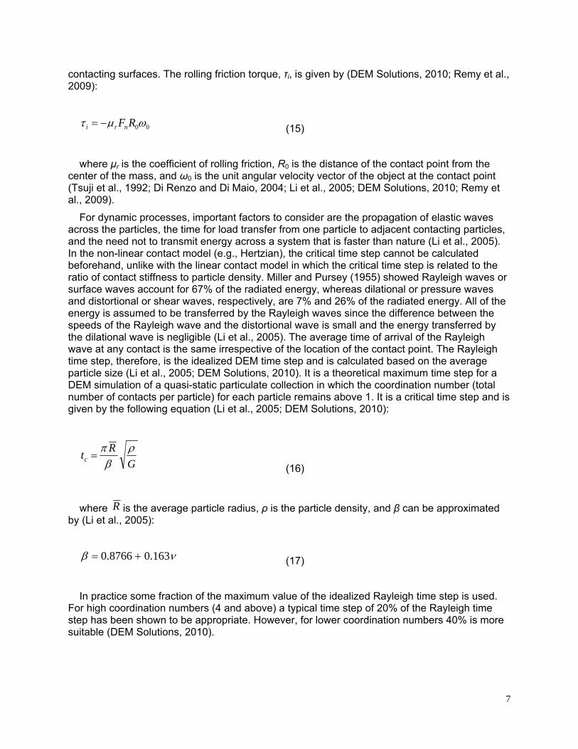
contacting surfaces. The rolling friction torque, τi, is given by (DEM Solutions, 2010; Remy et al., 2009):

00ωµτ RFnri −= (15)

where µr is the coefficient of rolling friction, R0 is the distance of the contact point from the center of the mass, and ω0 is the unit angular velocity vector of the object at the contact point (Tsuji et al., 1992; Di Renzo and Di Maio, 2004; Li et al., 2005; DEM Solutions, 2010; Remy et al., 2009).

For dynamic processes, important factors to consider are the propagation of elastic waves across the particles, the time for load transfer from one particle to adjacent contacting particles, and the need not to transmit energy across a system that is faster than nature (Li et al., 2005). In the non-linear contact model (e.g., Hertzian), the critical time step cannot be calculated beforehand, unlike with the linear contact model in which the critical time step is related to the ratio of contact stiffness to particle density. Miller and Pursey (1955) showed Rayleigh waves or surface waves account for 67% of the radiated energy, whereas dilational or pressure waves and distortional or shear waves, respectively, are 7% and 26% of the radiated energy. All of the energy is assumed to be transferred by the Rayleigh waves since the difference between the speeds of the Rayleigh wave and the distortional wave is small and the energy transferred by the dilational wave is negligible (Li et al., 2005). The average time of arrival of the Rayleigh wave at any contact is the same irrespective of the location of the contact point. The Rayleigh time step, therefore, is the idealized DEM time step and is calculated based on the average particle size (Li et al., 2005; DEM Solutions, 2010). It is a theoretical maximum time step for a DEM simulation of a quasi-static particulate collection in which the coordination number (total number of contacts per particle) for each particle remains above 1. It is a critical time step and is given by the following equation (Li et al., 2005; DEM Solutions, 2010):

GRtc

ρβπ

= (16)

where R is the average particle radius, ρ is the particle density, and β can be approximated by (Li et al., 2005):

νβ 163.08766.0 += (17)

In practice some fraction of the maximum value of the idealized Rayleigh time step is used. For high coordination numbers (4 and above) a typical time step of 20% of the Rayleigh time step has been shown to be appropriate. However, for lower coordination numbers 40% is more suitable (DEM Solutions, 2010).

8

PILOT-SCALE BOOT EXPERIMENT Validation tests were performed by handling soybeans in a pilot-scale B3 bucket elevator leg

(Universal Industries, Inc., Cedar Falls, Iowa).

GRAIN MATERIALS Two types of soybeans were used for the grain commingling tests in the B3 leg. Test material

1 was red colored soybeans with clear-hilum from a 2008 crop variety KS4702. Five bags of these red soybeans were purchased from Kansas State University (KSU) Agronomy Farm on January 30, 2009. Each bag had a mean mass of 25.7 kg (standard deviation (SD) = 0.14 kg). Test material 2 was clear or uncolored soybeans with brown- and black-hilum from 2008 crop. The clear soybeans were purchased from a local elevator on December 4, 2008, and were cleaned through a fanning mill at KSU Agronomy Farm on December 5, 2008. After cleaning, the clear soybeans were then transferred in five grain tote bags with a mean mass of 563.9 kg (SD = 84.07 kg) for each bag.

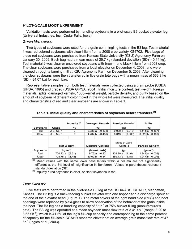
Representative samples from both test materials were collected using a grain probe (USDA GIPSA, 1995) and graded (USDA GIPSA, 2004). Initial moisture content, test weight, foreign materials, splits, damaged kernels, 1000-kernel weight, particle density, and purity based on the amount of soybean of different color mixed in the whole lot were measured. The initial quality and characteristics of red and clear soybeans are shown in Table 1.

Table 1. Initial quality and characteristics of soybeans before transfers.[a]

Red U.S. No. 1 0.337 a (0.131) 0.030 a (0.013) 1.114 a (0.167)Clear U.S. No. 1 1.207 b (0.486) 0.013 b (0.008) 0.329 b (0.103)

Red 700.72 a (3.21) 9.75 a (0.23) 138.90 a (4.46) 1.244 a (0.003)Clear 728.75 b (1.48) 10.09 b (0.34) 159.73 b (5.15) 1.247 b (0.004)

Soybeans

Impurity [b]

(%)00

Soybeans Grade

Damaged Kernels

(%)

(% wet basis)

Particle Density

(g·cm-3)

Mass of 1000 Kernels

Splits

(%)

Foreign Material

(%)

Moisture Content

(g)

Test Weight

(kg·m-3)

[a] Mean values with the same lower case letters within a column are not significantly different at the 5% level of significance in Bonferroni. Values in parentheses represent standard deviation (SD).

[b] Impurity = red soybeans in clear, or clear soybeans in red.

TEST FACILITY

Five tests were performed in the pilot-scale B3 leg at the USDA-ARS, CGAHR, Manhattan, Kansas. The B3 leg is a back-feeding bucket elevator with one hopper and a discharge spout at the end of the elevator head (Figure 1). The metal covers of the right hand side (RHS) and boot openings were replaced by plexi-glass to allow observation of the behavior of the grain inside the boot. The B3 leg has a handling capacity of 6 t·h-1 at 75% bucket filling (manufacturer’s data). The B3 leg was operated at a mean soybean mass flow rate of 3.41 t·h-1 (range: 3.20 to 3.65 t·h-1), which is 41.2% of the leg’s full-cup capacity and corresponding to the same percent of capacity for the full-scale CGAHR research elevator at an average grain mass flow rate of 47 t·h-1 (Ingles et al., 2003).

9

TEST PROCEDURE Figure 2 shows a schematic diagram of the grain flow during each grain transfer. The grain

transfers simulated the receiving operation of two consecutive grain types without additional (separate) cleaning of equipment between operations. Two types of soybeans of different color and hilum were used to easily identify grain commingling between grain loads.

Prior to each test, the B3 leg was allowed to self-clean by letting the leg to run on empty for 10 min. Compressed air was used through the right-hand side (RHS) opening of the leg (Figure 1) to clean the bucket cups while it is running. Grain residuals and impurities were vacuumed from the boot and other parts of the B3 leg. Before each transfer operation, the ambient and grain temperatures and ambient relative humidity were measured using a mercury thermometer and a psychrometer (model 3312-40, Cole-Parmer Instrument Co., Vernon Hills, Ill.), respectively. The stop of the hopper’s slide gate was checked and tightened for proper position giving the specific opening (width = 32.54 mm) for the flow rate of the test.

First Grain Transfer – Red Soybeans The red soybeans were transferred through the B3 leg initially. A bag of red soybeans was

poured into the hopper of the leg. A 125-L plastic container was positioned at the end of the spout to catch the red soybeans discharged from the head of the B3 leg. The B3 leg was switched on and the slide gate was opened to run the red soybeans. After the transfer of red soybeans, the B3 leg was allowed to continuously run for 5 min for self-cleaning prior to turning off.

After the red soybean handling, the residual grain heights were measured in the left-hand side (LHS) (i.e., from the top of the LHS opening to the grain) and in the RHS (i.e., from the boot floor to the height of the grain) of the B3 leg. The mean residual grain heights of red soybeans in the LHS and RHS from five tests were 123.2 (standard deviation, SD = 2.78) mm and 95.66 (SD = 0.91) mm, respectively.

The end of the spout connected to the head was transferred from the plastic container to the Gamet diverter-type (DT) sampler (Seedburo Equipment Co., Chicago, Ill.) to collect grain samples from the next soybean flow. The Gamet DT sampler was placed on top of a plastic hopper (1.07 x 1.37 x 1.59 m) collecting the remainder of the flow.

To accurately record the timing of each sampling, split-core AC current sensors (0-20 Amp model CTV-A, Onset HOBO, Bourne, Mass.) plugged directly into a 4-channel external input data logger (model HOBO H8) was attached to the control panel of the Gamet DT sampler. The clock on a laptop computer (model Sony Vaio PCG-Z505R, Sony Electronics, Inc., New York, N.Y.) was synchronized with the HOBO time.

Second Grain Transfer – Clear Soybeans Clear soybeans were transferred through the B3 leg after the red soybean transfer was

completed. The clear soybean lot in a tote bag was weighed on a digital platform scale (IQ Plus 310A, Rice Lake Weighing System, Inc., Rice Lake, Wisc.). After weighing, the tote bag was placed directly over the hopper of the B3 leg. The protective guard of the tote bag was positioned and opened to initiate filling of the hopper. The tube at the bottom of the tote bag was adjusted to prevent overflow. The height of the tote bag was adjusted to maintain the consistent flow of clear soybeans.

10

Figure 1. Pilot-scale boot without the LHS hopper.

Figure 2. Schematic diagram of grain flow represented by arrows in a B3 boot drawing

(without the LHS hopper).

boot opening (with plexiglass cover)

right hand side (RHS) opening (with plexiglass cover)

left hand side (LHS) opening where LHS hopper is mounted

Width (W) = 0.127 m

Length (L) = 0.305 m

Height (H) = 0.699 m

11

The slide gate of the hopper was opened at the same width for each transfer. The control panel of the Gamet DT sampler was turned on immediately after opening the slide gate. The stopwatch was started when the clear soybeans entered the boot. The real time for this start as displayed by the laptop clock (in seconds) was recorded. The RPM of the boot pulley shaft was measured with a digital tachometer (model 1726, AMETEK, Largo, Fla.).

GRAIN SAMPLING, SORTING, AND ANALYSIS Grain samples were diverted from the flow by the Gamet DT sampler every 15 s for the first 2

min (mean sample size [ n ] = 8, standard deviation [s.d.] = 1), every 30 s for the next 3 min ( n =6, s.d.=1), and every 60 s for the rest of the handling time ( n =4, s.d.=1). The mean sample size was dependent on the total mass of clear soybeans in each of the five grain tote bags. The transfer was completed when the last normal bucket cup scooping was seen through the plexi-glass cover. The real time for this complete transfer was recorded as displayed by the laptop clock. The total handling time was also recorded.

After the test, the B3 leg was allowed to self-clean for 5 min. The residual grain heights were measured in the LHS and RHS. The mean residual grain heights of clear soybeans in the LHS and RHS from five tests were 127.0 (SD = 0) mm and 96.09 (SD = 1.38) mm, respectively. The mean residual grain that was vacuumed from the boot and weighed from the five tests was 2.48 (SD = 0.02) kg.

Five replicated tests simulated a receiving operation of two consecutive grain types (red and clear soybeans) with only self-cleaning between operations. The grain samples collected by the Gamet DT sampler were weighed. The red soybeans were manually sorted from the clear soybeans. Dividing the sample mass from experiments by the computed soybean mass in a single bucket cup indicated that each sample represented three bucket cups.

The average commingling per given load mass (Ca) was computed by:

( )∑

∑×

⎟⎟⎠

⎞⎜⎜⎝

⎛⎟⎟⎠

⎞⎜⎜⎝

⎛+

××

=is

cr

ris

a tmmm

mtmC

&

&

(18)

where sm& is mass flow rate of soybeans (kg·s-1), ti is sampling time interval (s), mr is mass of red soybeans (kg), and mc is mass of clear soybeans (kg). The mass of grain in a bucket cup (in g·cup-1) was computed based on the mean mass flow rate of soybeans (in g·s-1) and the measured bucket cup rate (in cup·s-1).

The mass of grain in a bucket cup (mbc) in g·cup-1 was calculated using the following equation:

c

sbc f

mm&

= (19)

where sm& is the mean mass flow rate of soybeans in t·h-1 and fc is the measured bucket cup rate in cup·s-1 defined by:

12

c

bc s

vf = (20)

where vb is the boot belt speed in m·s-1 and sc is the bucket cup spacing in m·cup-1. The boot belt speed was computed as:

bbb Nrv π2= (21)

where rb is the radius of the boot pulley (and the belt thickness) in m and Nb is the boot pulley rpm.

PARTICLE MODEL The particle model developed by Boac et al. (2010) for soybeans was implemented in this

study. The model was a single-sphere particle model with the following properties: particle coefficient of restitution of 0.6, particle static friction of 0.45 for soybean-soybean contact (0.30 for soybean-steel interaction), particle rolling friction of 0.05, normal particle size distribution with standard deviation factor of 0.4, and particle shear modulus of 1.04 MPa. Table 2 lists the physical properties of soybeans and surfaces used in the simulation.

SIMULATION OF GRAIN COMMINGLING 3-D MODELING OF GRAIN COMMINGLING

A 3-D model based on the pilot-scale bucket elevator leg geometry (Model B3, Universal Industries, Inc., Cedar Falls, Iowa) in the experiments was used to determine grain commingling (Figure 1). The B3 pilot-scale leg is a back-feeding bucket elevator with one hopper and a discharge spout at the end of the elevator head. The elevator boot is the enclosed base of an elevator leg casing, where static grain, called residual grain, accumulates after material loading.

Geometries of the pilot-scale bucket elevator boot were drawn in a computer-aided design (CAD) software package (DS SolidWorks Corp., Concord, Mass.) and imported to establish model geometries in the DEM software (Figure 3). The material for bucket cups and enclosure of the leg was specified as steel and the belt was rubber (Table 2). The input parameters for a single-sphere particle model for the soybean kernel (Boac et al., 2010) are listed in Table 2.

Simulations were performed at 20% Rayleigh time steps (Table 2). The DEM modeling software used was EDEM 2.3 (DEM Solutions, Hanover, N.H.). The force-displacement law at contact points for all simulations was represented by a Hertz-Mindlin no-slip contact model (DEM Solutions, 2010).

13

Table 2. Input parameters for DEM modeling. Variable Symbol

Particle coefficient of restitution e 0.60 a 0.60 a 0.60 a 0.60 a

Particle coefficient of static friction (soybean on) µ s 0.45 a 0.45 a 0.30 a 0.50 a

Particle coefficient of rolling friction µ r 0.05 a 0.05 a 0.05 a 0.05 a

Particle size distribution PSD normal a normal a

Mean factor MF 1.0 a 1.0 a

Standard deviation factor SDF 0.4 a 0.4 a

Particle shear modulus, Pa G 1.04E+06 a 1.04E+06 a 7.00E+10 b, c, e 1.00E+06 b, d

Particle Poisson's ratio ν 0.25 a 0.25 a 0.30 b, c, e 0.45 b, d

Particle Young's modulus, Pa E 2.60E+06 a 2.60E+06 a 1.82E+11 b, c, e 2.90E+06 b, d

Particle density, kg·m-3 ρ 1243 f 1247 f 7800 b, c, e 9100 b, d

Particle mass, g m 0.1597 f 0.1389 f

Particle radius, mm R 3.13 g 2.985 g

Particle generation rate, particles/s 5,931 6,819 Calculated Rayleigh time step, s 3.71E-04 3.54E-04Simulation time step, s 7.08E-05 7.08E-05

Red Soybean Clear Soybean Steel Rubber

0n&

a Boac et al., 2010

b DEM Solutions, 2010 c Boresi and Schmidt, 2003 d Ciesielski, 1999 e Baumeister et al., 1978 f Measured values g Calculated values

14

(b)

Figure 3. Initial 3-D test model of pilot-scale boot with red soybeans.

H = 0.699 m

W = 0.127 m

L = 0.305 m

15

Simulation of an initial 3-D test model was performed first to establish basic model characteristics. In this initial simulation, red soybean particles were handled first in the boot geometries of the 3-D test model (Figure 3). The elevator leg was allowed to run until the residual grain stabilized. After handling red soybeans, the mass of residual grain was determined by extracting the particle mass remaining in the boot geometry. With red soybean particles as the residual grain in the 3-D leg geometry, clear soybean particles were run next for approximately 5 min in simulation time.

The total particle mass of red and clear soybeans were determined from each bucket cup. The average commingling data were computed based on equation 18 and plotted at time intervals matching the experiments.

In the validation experiment, discussed in the previous sections, the belt of the bucket elevator leg was not rigid and swayed away from the boot pulley making the gap between the bucket cups and the boot wall smaller; this smaller gap was termed as dynamic gap. In the initial 3-D test model, the belt was rigid making the gap wider (i.e., static gap = 28.95 mm), enabling some soybeans to slip back to the boot bottom without the bucket cup collecting them (Figure 4a).

The static gap in the initial 3-D test model with a rigid belt was reduced to the dynamic gap in the 3-D model matching the B3 boot. There were two dynamic gaps tested: (1) 14.48 mm, which was inclusive of the measured gap while the bucket cups were moving in the experiment (14.29 – 22.23 mm), and (2) 9.525 mm, which was the minimum measured gap observed when the bucket cups were at rest and would occur when the cups sway closest to the wall.

There are two ways to adjust for the dynamic gap in the CAD drawing of the boot geometry. One is to move the belt and bucket cups assembly towards the front loading side (i.e., right-hand side of the geometry) in the CAD drawing. The other is to put additional boot material, i.e., a secondary RHS wall placed at a certain distance (or dynamic gap) in between the center pulley and the original RHS wall of the boot geometry (Figure 4b). This was also incorporated in the CAD drawing of the boot geometry before importing it to EDEM. This latter method was followed because it did not affect the incoming flow of soybeans and it contributed to accurately matching the residual grain mass in the experiment.

The best dynamic gap for the 3-D model from the preliminary test simulation was 14.48 mm. It was closer to the realistic value when bucket cups are moving and gave an average flow rate of clear soybeans and average commingling simulation results closer to actual experimental results than the other tested dynamic gap value. This dynamic gap was implemented in the simulations of 3-D model matching the B3 boot.

Different dimensions of the gate opening of the LHS hopper (1/4-, 1/3-, 2/5-, 5/12-, 1/2-, 3/4-, fully-opened gate) were also tested. The best gate opening was 2/5-fully opened, (i.e., 50.8 mm) because it gave the flow rate matching that of the experiments. Preliminary simulations also investigated different filling times for the LHS hopper to accumulate the proper amount of clear soybeans in the LHS hopper. It was found that 15 s filling time for the LHS hopper was appropriate to maintain the flow rate desired for clear soybeans. These details were incorporated in the 3-D model matching the B3 boot.

16

(a)

(b)

Figure 4. (a) Initial 3-D test model showing static gap and (b) 3-D model showing dynamic gap.

L = 0.305 m

H = 0.699 m

W = 0.127 m

Static Gap = 28.95 mm

L = 0.305 m

H = 0.699 m

W = 0.127 m

Dynamic Gap = 14.48 mm .

17

Simulation of grain commingling in a 3-D model matching the B3 boot was performed in the same way as the initial 3-D test model. Red soybeans were handled first in the boot geometries and allowed to stabilize as a residual grain for 15 s. Then the mass of the residual grain was determined by extracting the particle mass remaining in the boot geometry.

The observed sudden surge of particles from the hopper when the slide gate was opened in the experiment was included in the 3-D model of the B3 boot. The particle surge flow stirs up more particles initially than would be simulated without the surge flow. To implement the sudden particle surge in the B3 boot model, a closed slide gate was modeled. With red soybean particles remaining in the 3-D boot geometry as the residual grain, clear soybeans were generated and allowed to accumulate in the LHS hopper for 15 s before opening the slide gate (Figure 5a). When the gate was opened, a sudden surge of particles was observed in the simulation (Figures 5b, 5c, and 5d). Clear soybeans were then continuously run in the boot for approximately 8 min in simulation time.

The average commingling data were computed based on equation 18 and plotted at time intervals matching the experiments. The trend of average commingling from the 3-D model of the B3 boot was compared with experimental data.

The start time for sampling was calculated based on the best estimated initial time simulating the experimental validation. The time for the soybeans to be scooped by bucket cups to the time they were collected in the Gamet DT sampler was measured to be 5.0 s. Simulation data times were adjusted accordingly.

The difficulty of matching the initial time in the experiments to that in the simulations was an important issue for the accuracy in time of predicted commingling. The time of initial particle uptake in the experiments was carefully timed with a stopwatch and then carefully matched to the initial uptake of particles in the 3-D simulation.

QUASI-2-D MODELING OF GRAIN COMMINGLING To simplify the model and reduce computational time, a quasi-2-D model was investigated for

the B3 pilot-scale bucket elevator boot. The same geometries of the B3 boot drawn in the CAD software were imported to establish model geometries in the quasi-2-D simulation.

Quasi-2-D models utilize a 3-D system but with only a fixed width slice of the 3-D geometry, usually equivalent to a given number of particle diameters. A quasi-2-D model is usually preferable to a true 2-D model because unlike a 2-D model, it can capture the 3-D effects of interacting spheres. Likewise, it is also preferable to a 3-D model because it reduces computational time (Boac et al., 2010).

To generate a quasi-2-D model of the pilot-scale boot, the dimension in the z-direction (i.e., width) of the boot was reduced by using periodic boundaries on both front and back walls. Periodic boundary conditions enable any particle leaving the domain in that direction to instantly re-enter on the opposite side (DEM Solutions, 2010), simulating infinite length in that direction, thereby eliminating wall effects and reducing the total number of particles inside the control volume. The elimination of wall effects, such as particle-on-wall friction, could potentially reduce simulation accuracy if those effects are large enough in the true 3-D case.

18

(a)

(b)

(c)

(d)

Figure 5. 3-D model of B3 boot with particles: (a) accumulating at the gate and (b, c, d) with surge flow.

H = 0.699 m

W = 0.127 m

L = 0.305 m

19

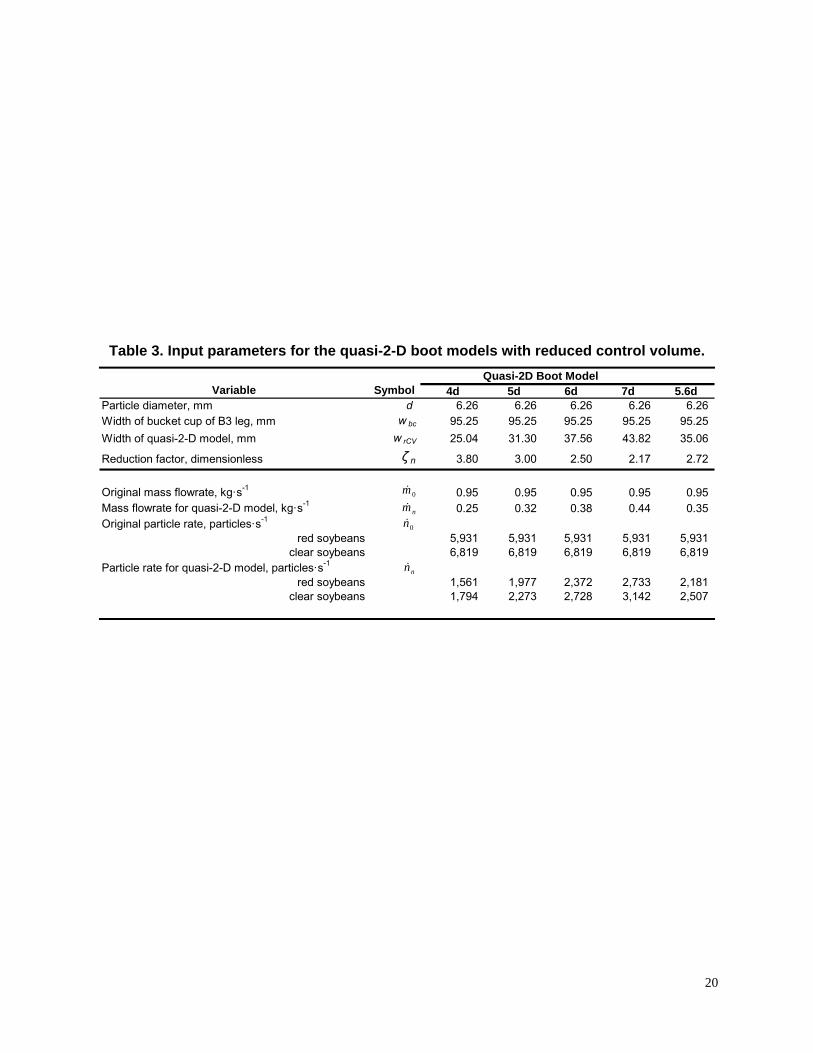
Preliminary tests of five quasi-2-D models were performed to determine the acceptable model for quasi-2-D simulation. The models had widths of from four to seven times the mean particle diameter (d) of red soybeans (i.e., 4d, 5d, 5.6d, 6d, 7d) (Table 3). The reduction factor, ζn, for each quasi-2-D model is defined as:

DQ

bcn w

w

2

=ζ (n = 4, 5, 5.6, 6, 7) (22)

where wbc is the original width of the bucket cup and wQ2D is the width of the quasi-2-D model (i.e., 4d, 5d, 5.6d, 6d, or 7d).

A single-sphere particle model with the same material and interaction properties of soybean used in the 3-D model was employed in the quasi-2-D models (Boac et al., 2010). The total number of particles created was also reduced based on the reduction factor (Table 3).

Similar to the 3-D modeling, red soybean particles were also handled first in the quasi-2-D model until the residual grain stabilized after a run time of 15 s (Figure 6a). Red soybeans were left as residual grain. Clear soybeans were allowed to accumulate in the LHS hopper for 15 s before opening the gate and allowing them to run for approximately 35 s (Figure 6b). Average commingling for each quasi-2-D model was computed based on equation 18. The trends of the average commingling results from the four quasi-2-D boot models were compared. The quasi-2-D model, which had the smallest reduced control volume with stable simulation and safety margin, was chosen to model the pilot-scale B3 boot.

Quasi-2-D simulation of the B3 boot was performed the same way as the 3-D model but with the chosen reduced control volume (i.e., equivalent to a given number of particle diameters). The timing of the start of sampling time, particle surge flow, and effective dynamic gap were included in the chosen quasi-2-D model. The best dynamic gap chosen in the 3-D model of the B3 boot was used initially as the effective gap in the quasi-2-D model. The trends of commingling data from the chosen quasi-2-D model of the B3 boot were compared with the 3-D model and experimental data. Table 4 summarized the levels of simulations performed in EDEM using 3-D and quasi-2-D models.

DATA ANALYSIS Statistical analysis was performed using the General Linear Model (GLM) procedure of SAS

statistical software (ver. 9.2, SAS Institute, Inc., Cary, N.C.). Basic descriptive statistics (i.e., mean and standard deviation) were determined for the parameters evaluated. Standard error of the model compared to experiment was computed for each model plot. Experimental data were compared with 3-D model and quasi-2-D model of the B3 boot at experimental sampling time intervals. Predicted results were compared with lower and upper limits of the 95% confidence interval of the experimental data.

20

Table 3. Input parameters for the quasi-2-D boot models with reduced control volume.

4d 5d 6d 7d 5.6dParticle diameter, mm d 6.26 6.26 6.26 6.26 6.26 Width of bucket cup of B3 leg, mm w bc 95.25 95.25 95.25 95.25 95.25 Width of quasi-2-D model, mm w rCV 25.04 31.30 37.56 43.82 35.06

Reduction factor, dimensionless ζ n 3.80 3.00 2.50 2.17 2.72

Original mass flowrate, kg·s-1 0.95 0.95 0.95 0.95 0.95 Mass flowrate for quasi-2-D model, kg·s-1 0.25 0.32 0.38 0.44 0.35 Original particle rate, particles·s-1

red soybeans 5,931 5,931 5,931 5,931 5,931 clear soybeans 6,819 6,819 6,819 6,819 6,819

Particle rate for quasi-2-D model, particles·s-1

red soybeans 1,561 1,977 2,372 2,733 2,181 clear soybeans 1,794 2,273 2,728 3,142 2,507

SymbolVariable Quasi-2D Boot Model

0m&

0n&

nn&

nm&

21

(a)

(b)

Figure 6. Quasi-2-D simulation during handling of (a) red and (b) clear soybeans.

W = 5.6d = 0.035 mm

H = 0.699m

L = 0.305 m

H = 0.699m

L = 0.305 m

W = 5.6d = 0.035 mm

22

Table 4. Summary of 3-D and quasi-2-D simulation levels. Model Features and Factors

Considered Remarks

Initial 3-D Model

- Static gap = 28.95 mm

- Performed to establish basic model characteristics.

- The belt was rigid making the gap between the bucket cups and the RHS boot wall wider, which enables some soybeans to slip back to the boot bottom without the bucket cup collecting them.

- No particle surge

- There was also no particle surge that pushed the red soybeans towards the RHS to mix properly with the clear soybeans.

3-D Model - Dynamic gaps: 14.48 mm and 9.525 mm

- Tested two dynamic gaps: (1) 14.48 mm, which was inclusive of the measured gap while the bucket cups were moving in the experiment (14.29 – 22.23 mm), and (2) 9.525 mm, which was the minimum measured gap when the bucket cups were at rest and would occur when the cups sway close to the wall.

- The best dynamic gap was 14.48 mm, which was closer to the realistic value when bucket cups are moving, closely matched average flow rate of clear soybeans, and gave average commingling simulation results closer to actual experimental results.

- Slide gate openings: 1/4-, 1/3-, 2/5-, 5/12-, 1/2-, 3/4-, fully-opened gate

- Tested different slide gate openings of the LHS hopper.

- The best gate opening was 2/5-fully opened, (i.e., 50.8 mm) because it gave the flow rate matching that of the experiments.

- LHS hopper filling times: 5s, 10s, 15s

- Tested different filling times for the LHS hopper to accumulate the proper amount of clear soybeans in the LHS hopper.

- It was found that 15 s filling time for the LHS hopper was appropriate to maintain the flow rate desired for clear soybeans.

- With particle surge flow

- The observed sudden surge of particles from the hopper when the slide gate was opened in the experiment was implemented in the 3-D model.

- To implement the sudden particle surge in the 3-D model, the slide gate was closed first, red soybeans were left to accumulate in the LHS hopper for 15 s, and then the slide gate was opened. When the gate was opened, a sudden surge of particles was observed in the simulation.

- The particle surge flow stirs up more particles initially than would be simulated without the surge flow, achieving commingling results that closely matched the experiments in the long run.

Quasi 2-D Models

- Reduced control volumes: 4d, 5d, 5.6d, 6d, 7d

- Performed to determine the acceptable model with reduced control volume.

- The quasi-2-D model, which had the smallest reduced control volume with stable simulation and safety margin for modeling, was chosen to model the pilot-scale B3 boot.

Quasi 2-D (5.6d) Model

- Wider “effective gap” to account for edge effects missing in quasi-2-D

- LHS hopper filling times: 5s, 10s, 15s

- Using effective dynamic gap (14.48 mm) in the quasi-2-D (5.6d) model posed a problem, which may be explained by the edge effects in the 3-D model, but not in quasi-2-D (5.6d) model due to the reduced control volume.

- Tested for wider “effective gap” that allows more grain to return to boot from missing edge effects in quasi-2-D model.

- Different filling times of the LHS hopper to determine the resulting particle surge that would match predicted commingling with that of the experiments.

23

RESULTS AND DISCUSSION EXPERIMENTAL RESULTS

Average commingling for the five tests started at 4.25% during the first 5 s, decreased to 2.20% after 21 s, to 0.42% after 3.2 min, and eventually reached 0.20% after 7.7 min. The end result (0.20%) was within the published average cumulative commingling for combined effect of pit and elevator boot for the full-scale CGAHR research elevator, which was 0.18% (Ingles et al., 2003) and the elevator leg only for a full-scale commercial facility, which was 0.23% (Ingles et al., 2006). Figure 7 shows 95% confidence interval (C.I.) limits for the average commingling and was used to compare predicted results of simulation models.

From the experiments, the mean mass flow rate for soybeans ( sm& ) was measured as 3.41 t·h-1 (0.95 kg·s-1). The mean boot pulley rpm (Nb) and radius of the boot pulley, including belt thickness (rb), were 203.7 rpm and 0.0535 m, respectively. These values gave a boot belt speed (vb) of 1.141 m·s-1. The bucket cup spacing (sc) and frequency (fc) were 0.08255 m·cup-1 and 13.82 cups·s-1, respectively, resulting in mass of grain in a bucket cup (mbc) of 68.54 g·cup-1. These data were incorporated in the simulations using the 3-D model of the B3 pilot-scale boot. The gap between the bucket cups and the right-hand sidewall of the boot was set to 14.48 mm, within the range of the measured dynamic gap as discussed above.

0.0

0.5

1.0

1.5

2.0

2.5

3.0

3.5

4.0

4.5

5.0

0 50 100 150 200 250 300 350 400 450 500 550 600 650 700Time (s)

Gra

in C

omm

ingl

ing

(%)

Experiment - Average - 95% C.I. Lower Limit

Experiment - Average - 95% C.I. Upper Limit

Figure 7. Average commingling from experiments showing 95% confidence interval (C.I.)

limits.

24

PREDICTED GRAIN COMMINGLING WITH 3-D BOOT MODEL Initial 3-D Test Model

Predicted average commingling from the initial 3-D test model followed the trend of but over predicted experimental data (Figure 8). The over prediction can be due to the static gap between the bucket cups and the RHS wall of the boot. The wider static gap allowed some soybeans to slip back to the boot bottom without the bucket cup collecting them early in the experiment. The absence of particle surge of the clear soybeans after the gate was opened for the second grain may also contribute to over prediction of commingling. The gap between the bucket cups and RHS wall of the boot, and the absence of particle surge during the onset of the clear soybean flow were further refined in the succeeding simulations.

0.0

1.0

2.0

3.0

4.0

5.0

6.0

7.0

8.0

0 20 40 60 80 100 120 140 160 180 200 220 240 260 280 300

Time (s)

Gra

in C

omm

ingl

ing

(%)

Initial 3-D Test Model - Average (Matching Experimental Time)

Experiment - Average - 95% C.I. Lower Limit

Experiment - Average - 95% C.I. Upper Limit

Figure 8. Average commingling data from initial 3-D test model compared with 95% C.I.

limits of the experiments, plotted at time intervals matching the experiments.

25

Complete 3-D Model for B3 Boot Preliminary simulations in the 3-D model were performed to evaluate the most appropriate

model details for the B3 boot. The dynamic gap between the bucket cups and the RHS boot wall was investigated and the best one was the 14.48-mm gap because it was closer to the realistic value when bucket cups are moving. Furthermore, it closely matched the average flow rate of clear soybeans, and gave average commingling simulation results closer to experimental results. Different openings of the slide gate of the LHS hopper were also tested as well as various filling times for the LHS hopper with clear soybeans. The best gate opening size was 2/5-fully opened, (i.e, 50.8 mm) and the best filling time for the LHS hopper to accumulate clear soybeans was 15 s. These combinations of model details were incorporated in the complete 3-D model because they allow the simulation to maintain the desired flow rate for clear soybeans that matched the experiments.

Figure 9 shows the average commingling results of the best 3-D model (3-D Model 1), and the second best 3-D model (3-D Model 2), computed at time intervals matching the experiments. The 3-D Model 2 gave a better standard error of the model compared to experiment (s.e. = 0.82) than the 3-D Model 1 (s.e. = 1.50). Predicted commingling values for the 3-D Model 2 were within the 95% confidence limits of experimental data during the first 100 s; however, they were greater than experimental values at later times. Thus, 3-D Model 1 was chosen as the best 3-D model because at times longer than 100 s, it closely matched the experimental average commingling. Predictions at longer times were considered more important than during the initial 100 s because those at longer times represent the total commingling for the run, which is of greater interest in field operations than the initial values alone.

0.0

0.5

1.0

1.5

2.0

2.5

3.0

3.5

4.0

4.5

5.0

0 50 100 150 200 250 300 350

Time (s)

Ave

rage

Com

min

glin

g (%

)

Experiments - 95% C.I. Lower Limit

Experiments - 95% C.I. Upper Limit

3-D Model 1 (dynamic gap=14.48mm, 2/5-opened gate, LHS hopper filling 15s) [s.e. = 1.50]

3-D Model 2 (dynamic gap=14.48mm, 2/5-opened gate, LHS hopper filling 5s) [s.e. = 0.82]

Figure 9. Average commingling from 3-D Models 1 and 2 compared with 95% C.I.

limits of the experiments, plotted at time intervals matching the experiments.

26

PREDICTED GRAIN COMMINGLING WITH QUASI-2-D BOOT MODEL Predicted commingling results of quasi-2-D models with different widths or reduced control

volumes (i.e., 4-mean particle diameter (4d), 5d, 6d, and 7d) did not vary much (Figure 10), except for the quasi-2-D model (4d). The quasi-2-D (4d) model did not perform well in the simulation due to instability of the system in the reduced domain. This may result from issues such as the side of a large particle (from one side of the periodic boundary) touching another side of the same particle (on the other side of the periodic boundary), since the periodic boundary conditions enable any particle leaving the domain in that direction to instantly re-enter on the opposite side (DEM Solutions, 2010). Forces from contact of the particle with itself are expected to be unpredictable, thus, making the system unstable. This is also similar to putting a particle into a container of size smaller than the particle size. The system will be unpredictable and the particles would be unstable, which was what happened in the quasi-2-D (4d) model.

All quasi-2-D models beginning with 5d up to 7d were stable in the simulations. Their results appear to be invariant with reduction factor, ζn < 3.00 (i.e., quasi-2-D (5d) model in table 3) and so the ζn = 2.72 (i.e., the quasi-2-D (5.6d) model) was selected to be slightly conservative because it gave a safety margin for modeling and was the equivalent of a 4dmax criterion recommended by the software company2. The invariant results are in agreement with previous studies modeling hopper flow in a solar silo (Joseph et al., 2000) and segregation in hopper flow (Ketterhagen et al., 2008) with periodic boundaries separated by only a smaller value of grain radii. The quasi-2-D (5.6d) model was tested and found that it was stable in the simulations and relatively faster than the quasi-2-D (6d) model. Thus, the quasi-2-D (5.6d) model was implemented for the B3 boot simulations as a faster alternative to the 3-D model.

0.0

2.0

4.0

6.0

8.0

10.0

12.0

14.0

16.0

18.0

20.0

0 2 4 6 8 10 12 14 16 18 20 22 24 26 28 30 32 34 36

Time (s)

Gra

in C

omm

ingl

ing

(%)

Quasi-2-D (5d)

Quasi-2-D (6d)

Quasi-2-D (7d)

Figure 10. Average commingling from preliminary quasi-2-D models with reduced control volume. [Note: The quasi-2-D (4d) model was unstable.]

2 Oleh Baran (DEM Solutions, Inc.), personal communications, October 19, 2009.

27

Including the particle surge and using a dynamic gap of 14.48 mm in the best 3-D model predicted commingling better than not including these refinements (Figure 9). However, following the dynamic gap of the 3-D model and applying it in the quasi-2-D (5.6d) model under predicted the commingling (Figure 11). This may be explained by the edge effects that are in the 3-D model, but not in the quasi-2-D (5.6d) model due to the reduced control volume. Figure 12 shows the quasi-2-D (15d) model, 15d is the full bucket cup width, in which the effective gap was wider than the dynamic gap of the best 3-D model. The wider “effective gap” allows space for more grain to return to the boot, compensating for missing edge effects in the quasi-2-D model. The same applies to the quasi-2-D (5.6d) model. The correct effective gap used for the quasi-2-D (5.6d) model was equal to the original static gap (28.95 mm). The inclusion of the correct effective gap and particle surge flow in the quasi-2-D (5.6d) model predicted the closest value of average commingling to the results of the best 3-D model (Figure 13).

Different filling times of the LHS hopper to vary the particle surge were also tested. Using a 5-s filling time, the quasi-2-D Model 1 matched the experimental average commingling for the first 70 s, and then over predicted the commingling after that time. With a 15-s filling time similar to that in the 3-D Model 1, the quasi-2-D Model 2, under predicted the average commingling during the first 100 s but the results tended to match the experimental average commingling after that time. This may be due to more clear soybeans commingling with the red soybeans in the beginning of the run, thus, under predicting the commingling during the first few seconds. The 10-s LHS hopper filling time in the quasi-2-D Model 3 showed results that were between the 5 and 15 s filling times. Further improvements in the quasi-2-D model might be achieved by testing different LHS hopper filling times between 5 and 15 s and running the simulation longer to match the experimental times. Other improvements may be achieved by predicting the effect of vibration motions in the residual grain mass and height and investigating different particle properties (i.e., soybean material and interaction properties as well as its particle size distribution) in the system.

The quasi-2-D (5.6d) models reduced simulation run time by 72% to 74% compared to the 3-D model with both models being run on the same workstation computer. It is postulated that a greater reduction in time will be achieved in the full-scale boot using a quasi-2-D (5.6d) model since a full scale boot will have a boot width much greater than the 15d of the B3 leg boot.

28

0.0

0.5

1.0

1.5

2.0

2.5

3.0

3.5

4.0

4.5

5.0

0 20 40 60 80 100 120 140 160 180 200

Time (s)

Ave

rage

Com

min

glin

g (%

)

Experiments - 95% C.I. Lower Limit

Experiments - 95% C.I. Upper Limit

3-D Model 1 (dynamic gap=14.48mm, 2/5-opened gate, LHS hopper filling 15s) [s.e. = 1.50]

Quasi-2-D (5.6d) Model 1 (dynamic gap=14.48mm, 2/5-opened gate, LHS hopper filling 15s) [s.e. = 4.24]

Figure 11. Average commingling from 3-D and quasi-2-D (5.6d) models with the same

dynamic gap.

Figure 12 . Dynamic and effective gaps illustration for full and reduced control volumes.

Dynamic Gap Effective Gap Effective Gap

29

0.0

0.5

1.0

1.5

2.0

2.5

3.0

3.5

4.0

4.5

5.0

0 50 100 150 200 250 300 350 400 450

Time (s)

Ave

rage

Com

min

glin

g (%

)Experiments - 95% C.I. Lower Limit

Experiments - 95% C.I. Upper Limit

3-D Model 1 (dynamic gap=14.48mm, 2/5-opened gate, LHS hopper filling 15s) [s.e. = 1.50]

Quasi-2-D (5.6d) Model 1 (static gap = 28.95mm, LHS hopper filling 5 s) [s.e. = 1.28]

Quasi-2-D (5.6d) Model 2 (static gap = 28.95mm, LHS hopper filling 15 s) [s.e. = 2.15]

Quasi-2-D (5.6d) Model 3 (static gap = 28.95mm, LHS hopper filling 10 s) [s.e. = 1.85]

Figure 13. Average commingling from quasi-2-D models using effective gap at different

LHS hopper filling times.

Conclusion Grain commingling in a pilot-scale bucket elevator boot was modeled in three-dimensional (3-

D) and quasi-two-dimensional (quasi-2-D) discrete element method (DEM) simulations. Experiments with grain commingling were performed to validate the DEM models with a pilot-scale boot using soybeans as the test material. The following conclusions were drawn from the research:

• Experimental data showed that mean average commingling started at 4.25% during the first 5 s, decreased to 2.20% after 21 s, went to 0.42% after 3.2 min, and eventually went to 0.20% after 7.7 min. The end result was within the published range of average cumulative commingling values for full size bucket elevator legs.

• Predicted commingling from the initial 3-D pilot-scale boot model generally followed the trend of experimental data, but over predicted the commingling. Refinements of the 3-D model showed that the best 3-D model had an effective dynamic gap between the bucket cups and boot wall of 14.48-mm, with slide gate 2/5-opened, (i.e, 50.8 mm), and the filling time for the LHS hopper to accumulate clear soybeans was 15 s.

• Comparison of predicted average commingling of five quasi-2-D boot models with reduced control volumes showed the quasi-2-D (5.6d) model provided the best option in reducing computational time; it reduced computational time by 72% to 74% compared to the 3-D model.

30

• Refinement of the quasi-2-D (5.6d) model by accounting for the sudden surge of particles during entry and correcting for the effective dynamic gap between the bucket cups and the boot wall better predicted commingling than did the models without those refinements included.

This study showed that grain commingling in a bucket elevator boot system can be simulated in 3-D and quasi-2-D DEM models, giving results that agreed with experimental data. Results of this study can be used to predict impurity levels and improve grain handling, which can help farmers and grain handlers reduce costs during transport and export of grains.

ACKNOWLEDGEMENTS The research was supported by USDA (CRIS No. 5430-43440-007-00D) and by the Kansas

Agricultural Experiment Station (Contribution No. 12-203-A). The technical support of Dr. Oleh Baran (DEM Solutions), Dr. Jasper Tallada (formerly USDA ARS CGAHR), Stephen Cole (DEM Solutions), Mark Cook (DEM Solutions), Dr. Sam Wai Wong (formerly DEM Solutions), and Dr. David Curry (DEM Solutions), and the assistance provided by Mr. Dennis Tilley (USDA ARS CGAHR) in conducting the experiments are highly appreciated. We also want to thank Dr. Bill Schapaugh (KSU), Vernon Schaffer (KSU), Shaun Winnie (KSU), and Dustin Miller (Kaufmann Seeds), for the fanning mill and soybean samples.

REFERENCES Baumeister, T., E. A. Avallone, and T. Baumeister III. 1978. Marks’ Standard Handbook for

Mechanical Engineers. 8th ed. New York: McGraw-Hill Book Co.

Boac, J. M., M. E. Casada, R. G. Maghirang, and J. P. Harner III. 2010. Material and interaction properties of selected grains and oilseeds for modeling discrete particles. Transactions of ASABE 53(4): 1201-1216.

Boresi, A. P. and R. J. Schmidt. 2003. Advanced Mechanics of Materials. 6th ed. New York: Wiley and Sons.

Bucchini, L. and L. R. Goldman. 2002. Starlink corn: a risk analysis. Environmental Health Perspectives 110(1): 5-12.

Ciesielski, A. 1999. An Introduction to Rubber Technology. United Kingdon: Rapra Technology, Ltd.

Cundall, P. A. 1971. A computer model for simulating progressive large-scale movements in blocky rock systems. In Proceedings of the Symposium of the International Society of Rock Mechanics, Vol. 1, Paper No. II-8: 132-150. Nancy, France: International Society of Rock Mechanics.

Cundall, P. A., and O. D. L. Strack. 1979. A discrete numerical model for granular assemblies. Geotechnique 29(1):47-65.

DEM Solutions. 2010. EDEM 2.3 User Guide. Hanover, N.H.: DEM Solutions (USA), Inc. 137p.

Di Renzo, A., and F. P. Di Maio. 2004. Comparison of contact-force models for the simulation of collisions in DEM-based granular flow codes. Chemical Engineering Science 59(3): 525-541.

Di Renzo, A., and F. P. Di Maio. 2005. An improved integral non-linear model for the contact of particles in distinct element simulations. Chemical Engineering Science 60(5): 1303-1312.

31

Fazekas, S., J. Kertesz, and D. E. Wolf. 2005. Piling and avalanches of magnetized particles. Physical Review E 71(6): 0613031-0613039.

Fillot, N., I. Iordanoff, and Y. Berthier. 2004. A granular dynamic model for the degradation of material. Transactions of the ASME, Journal of Tribology 126(3): 606-614.

Goda, T. J., and F. Ebert. 2005. Three-dimensional discrete element simulations in hoppers and silos. Powder Technology 158(1-3): 58-68.

Greenlees, W. J., and S. C. Shouse. 2000. Estimating grain contamination from a combine. ASAE Paper No. MC00103. St. Joseph, Mich.: ASAE.

Hanna, H. M., D. H. Jarboe, and G. R. Quick. 2006. Grain residuals and time requirements for combine cleaning. ASAE Paper No. 066082. St. Joseph, Mich.: ASAE.

Hart, R., P. A. Cundall, and J. Lemos. 1988. Formulation of a three-dimensional distinct element method, part II: mechanical calculations for motion and interaction of a system composed of many polyhedral blocks. International Journal of Rock Mechanics and Mining Sciences and Geomechanics Abstracts 25(3):117-125.

Hirai, Y., M. D. Schrock, D. L. Oard, and T. J. Herrman. 2006. Delivery system of tracing caplets for wheat grain traceability. Applied Engineering in Agriculture 22(5): 747-750.

Ingles, M. E. A., M. E. Casada, and R. G. Maghirang. 2003. Handling effects on commingling and residual grain in an elevator. Transactions of the ASAE 46(6): 1625-1631.

Ingles, M. E. A., M. E. Casada, R. G. Maghirang, T. J. Herrman, and J. P. Harner, III. 2006. Effects of grain-receiving system on commingling in a country elevator. Applied Engineering in Agriculture 22(5): 713-721.

Joseph, G. G., E. Geffroy, B. Mena, O. R. Walton, and R. R. Huilgol. 2000. Simulation of filling and emptying in a hexagonal-shape solar grain silo. Particulate Science and Technology 18(4): 309-327.

Kamrin, K., C. H. Rycroft, and M. Z. Bazant. 2007. The stochastic flow rule: a multi-scale model for granular plasticity. Modelling and Simulation in Materials Science and Engineering 15(4): 449-464.

Kawaguchi, T., M. Sakamoto, T. Tanaka, and Y. Tsuji. 2000. Quasi-three-dimensional numerical simulation of spouted beds in cylinder. Powder Technology 109(1-3): 3-12.

Ketterhagen, W. R., J. S. Curtis, C. R. Wassgren, and B. C. Hancock. 2008. Modeling granular segregation in flow from quasi-three-dimensional, wedge-shaped hoppers. Powder Technology 179(3): 126-143.

Kilman, S., and J. Carroll. 2002. Monsanto says crops may contain genetically-modified canola seed. The Wall Street Journal. Available at: http://www.connectotel.com/ gmfood/monsanto.html. Accessed 15 May 2008.

Li, Y., Y. Xu, and C. Thornton. 2005. A comparison of discrete element simulations and experiments for ‘sandpiles’ composed of spherical particles. Powder Technology 160(3): 219-228.

Masson, S., and J. Martinez. 2000. Effect of particle mechanical properties on silo flow and stresses from distinct element simulations. Powder Technology 109:164-178.

Miller, G. F., and H. Pursey. 1955. On the partition of energy between elastic waves in a semi-infinite solid. Proceedings of the Royal Society of London Series A: Mathematical and Physical Sciences 233(1192): 55-69.

32

Mindlin, R. 1949. Compliance of elastic bodies in contact. Journal of Applied Mechanics 16: 259-268.

Mindlin, R. D., and H. Deresiewicz. 1953. Elastic spheres in contact under varying oblique forces. Transactions of ASME, Series E. Journal of Applied Mechanics 20: 327-344.

Raji, A. O., and J. F. Favier. 2004a. Model for the deformation in agricultural and food particulate materials under bulk compressive loading using discrete element method, part I: theory, model development and validation. Journal of Food Engineering 64:359-371.

Raji, A. O., and J. F. Favier. 2004b. Model for the deformation in agricultural and food particulate materials under bulk compressive loading using discrete element method, part II: compression of oilseeds. Journal of Food Engineering 64:373-380.

Remy, B., J. G. Khinast, and B. J. Glasser. 2009. Discrete element simulation of free-flowing grains in a four-bladed mixer. AIChE Journal 55(8): 2035-2048.

Samadani, A., and A. Kudrolli. 2001. Angle of repose and segregation in cohesive granular matter. Physical Review E 64(5): 513011-513019.

Shimizu, Y., and P. A. Cundall. 2001. Three-dimensional DEM simulations of bulk handling by screw conveyors. Journal of Engineering Mechanics 127(9):864-872.

Sudah, O. S., P. E. Arratia, A. Alexander, and F. J. Muzzio. 2005. Simulation and experiments of mixing and segregation in a tote blender. Journal of American Institute of Chemical Engineers 51(3): 836-844.

Sykut, J., M. Molenda, and J. Horabik. 2008. DEM simulation of the packing structure and wall load in a 2-dimensional silo. Granular Matter 10(4): 273-278.

Takeuchi, S., S. Wang, and M. Rhodes. 2008. Discrete element method simulation of three-dimensional conical-based spouted beds. Powder Technology 184(2): 141-150.

Theuerkauf, J., S. Dhodapkar, and K. Jacob. 2007. Modeling granular flow using discrete element method – from theory to practice. Chemical Engineering 114(4): 39-46.

Tsuji, Y., T. Tanaka, and T. Ishida. 1992. Lagrangian numerical simulation of plug flow of cohesionless particles in a horizontal pipe. Powder Technology 71(3): 239-250.

US FDA. 2006. Strategic Partnership Program Agroterrorism (SPPA) Initiative. First Year Status Report. September 2005 - June 2006. Silver Spring, Md.: U.S. Food and Drug Administration. Available at: http://www.cfsan.fda.gov/~dms/agroter5.html. Accessed 15 May 2007.

USDA GIPSA. 1995. Grain Inspection Handbook, Book I, Grain Sampling. Washington, D.C.: USDA Grain Inspection, Packers, and Stockyards Administration, Federal Grain Inspection Service.

USDA GIPSA. 2004. Grain Inspection Handbook, Book II, Grain Grading Procedures. Washington, D.C.: USDA Grain Inspection, Packers, and Stockyards Administration, Federal Grain Inspection Service.

Wightman, C., M. Moakher, F. J. Muzzio, and O. R. Walton. 1998. Simulation of flow and mixing of particles in a rotating and rocking cylinder. Journal of American Institute of Chemical Engineers 44(6): 1266-1276.

Zhou, Y. C., B. H. Xu, A. B. Yu, and P. Zulli. 2001. Numerical investigation of the angle of repose of monosized spheres. Physical Review E: Statistical Physics, Plasmas, Fluids, and Related Interdisciplinary Topics 64(2): 0213011-0213018.