3: linear circuit analysis - hamblen.ece.gatech.eduhamblen.ece.gatech.edu/3710/ch3.pdf · x3:...

§3: Linear Circuit Analysis

§3.0 Introduction§3.1 Linear Systems§3.2 Superposition§3.3 Node-Voltage Analysis§3.4 Mesh-Current Analysis§3.5 Equivalent Circuits§3.6 Thevinin Equivalents§3.7 Norton Equivalents§3.8 Source Transformations§3.9 Maximum Power Transfer§3.10 Equivalent Resistance Revisited§3.11 Examples§3.12 Summary

§3.0 Introduction

When a carpenter works on a house or a mechanic tunes an engine, they each have many tools and various options forcompleting their tasks. Most tasks are straightforward: the carpenter uses a hammer to pound in nails, and the mechanic usesa specially designed wrench to remove the head gasket. Other tasks are slightly more ambiguous and require more information.Consider the carpenter working on a doorframe. Whether he chooses to use a hand saw, a power saw, or a pocket knife dependson the precision required, the number of doorframes to be built, and quite possibly the tools he has immediately available. Themechanic may have even more trouble in determining whether to use a half-inch or 13mm wrench for tightening an assembly.

The analysis methods presented in this chapter will provide you with a toolbox capable of tackling almost any linear DC circuit.The various methods will invariably terminate at the same answer, but some are clearly more efficient in solving particular circuits.Our goal is to construct both the toolbox and an understanding for what problems each tool is effective. More importantly, thesetools will provide you with the necessary preperation to analyze more complex circuits: those containing diodes, transistors, anddigital logic.

Beginning with simple applications of Ohm’s and Kirchoff’s laws, we will use equivalent impedances and dividers to lay thefoundation for our remaining circuit analyses. Larger circuits using both current and voltage dividers will create the framework.The properties of basic linear systems will allow us to perform analyses by superposition and Node/Mesh equations, furtherfleshing out our options. The last analysis step will be to create simple circuit equivalents for any linear circuit, thus completingour toolbox. Finally, we will address the various methods in a general setting and demonstrate a few tricks that can be used toview the problems more easily.

Where possible, we will demonstrate multiple methods in analyzing the circuits: you need only pick the one with which youfeel most comfortable. The benefit of solving a circuit multiple ways lies in the ability to check your answers–you can be prettywell certain that you are correct when you solve by completely different methods and obtain the same solution.

We will begin with a simple example to determine an output voltage given a DC input voltage as shown in Figure 3.1.

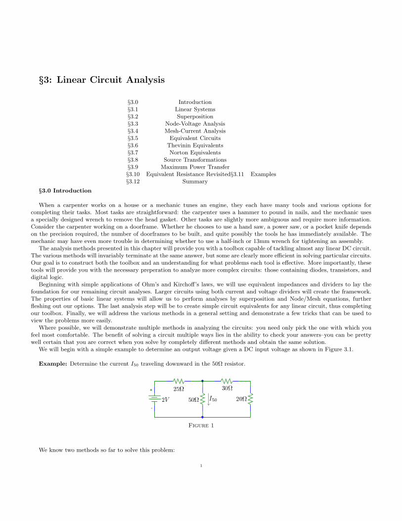
Example: Determine the current I50 traveling downward in the 50Ω resistor.

Figure 1

We know two methods so far to solve this problem:

1

2

1. We may determine the equivalent resistance looking to the right from the voltage source to then find the total currententering the collection of resistors. Application of a current divider then gives the current through the 50 Ω resistor.

Method 1: Req = 25 + 50‖(30 + 20) = 50 Ω

IT =2V

50Ω= 40 mA

I50 =(30 + 20)

(30 + 20) + 50IT = 20 mA

Figure 2

2. We may combine the 20, 30, and 50 Ohm resistors as an equivalent and then find the voltage across the equivalent (sameas the voltage across the 50Ω resistor). Simple application of Ohm’s law then gives us the current.

Method 2: Rcomb = 50‖(30 + 20) = 25Ω

Vcomb =Rcomb

Rcomb + 25(2V ) = 1 V

I50 =Vcomb

50Ω= 20 mA

Figure 3

In many ways, this is a very typical problem to solve: a circuit containing one source and perhaps four or five resistors. Let’s tryanother, more difficult, example that verifies the conservation of energy principle: all energy dissipated by a resistor is generatedby the source.

Example: Verify the conservation of energy in the circuit shown in Figure 3.4.

3

Figure 4

We use a combination of dividers and Ohm’s law applications to calculate the currents and the power dissipated.Current calculations:

I10Ω =1V

10Ω= 100 mA I15Ω =

1V

(15 + 6‖30) Ω=

1V

20Ω= 50 mA

I6Ω =30

30 + 6· I15Ω = 41.67 mA I30Ω =

6

30 + 6· I15Ω = 8.33 mA I1V = I10Ω + I15Ω = 150 mA

Power calculations:

P1V = (1V )(150mA) = 150 mW P6Ω = I26 (6Ω) = 10.41 mW P10Ω = I

210(10Ω) = 100 mW

P15Ω = I215(15Ω) = 37.5 mW P30Ω = I

230(30Ω) = 2.08 mW

A fully labeled circuit is shown in Figure 3.5.

Figure 5

To verify that the conservation of energy holds, compare the power generated by the voltage source to the sum of powersdissipated in the resisters.

150 mW.= (10.41 + 100 + 37.5 + 2.08) mW

Notice that there is an implicit assumption in this last step: we have shown that the powers are equal, but not the energy! Understeady-state conditions, the rate of energy into a circuit (the power) is constant and therefore the conservation of instantaneouspower implies conservation of energy over any time-scale.

§3.1: Linear Systems

One of the most common models studied in engineering is the linear system. The generic linear system is characterized by theproperty of linearity, which requires that the output is a weighted sum of the inputs. Figure 3.6 shows the block diagram of abasic linear system: for inputs x1, x2, ..., xn there are corresponding outputs y1, y2, ..., yn.

4

Figure 6

While this definition sounds trivial, answer the following question: is f(x) = x + 1 a linear system? Actually, no! Plotting thefunction on a set of axes as shown in Figure 3.7, you will see the answer jump out at you.

Figure 7

If we scale an input, say αx1, then the output is the same multiple times the corresponding output, αy1. Likewise, if we addtwo inputs and process them simultaneously, say x1 + x2, then the output is the corresponding sum y1 + y2.

Now, let’s return to the question of whether f(x) = x + 1 qualifies as a linear system: consider the three values f(0) = 1,f(1) = 2, and f(2) = 3. If f(x) was linear, then f(0 + 1) = f(0) + f(1), but 2 6= 1 + 2 = 3. Further, if f(x) were linear thenf(2 · 1) = 2 · f(1) which is again contradicted. The only conclusion is that f(x) = x + 1 is nonlinear, despite being a line; a lineneed not be mathematically linear! If the line happens to pass through the origin, then it will be linear.

Combining the properties discussed, we obtain the system response

yk = ck · xk ∀k ∈ N

succinctly stated as: “the output is a weighted sum of the inputs.” Two important characteristics of the linear system tonotice are that a zero input always corresponds to a zero output and that the weighting terms, ck, do not depend on any of theother inputs.

§3.2: Superposition

The bridge between mathematical definitions of linear systems and electrical circuits is a circuit technique called superposition.We will consider many circuits in this chapter, all of which are linear systems: the inputs of the circuit as a linear system arevoltage and current sources, and the outputs are any of the node voltages or currents in the circuit elements. A process calledsuperposition entails activating one source at a time and zeroing all others, allowing us to determine the response of the linearsystem (find each ck). Adding the contributions from each of these voltage and current sources, we will then be able to obtain theoverall response of our linear circuits. The limitation will be that we can only use superposition to determine linear quantities:power calculations (quadratic), diode calculations (exponential), and transistor analyses (mixture) will require additional methods.

Example: Use superposition to determine the current in the 5Ω resistor shown in Figure 3.8.

5

Figure 8

Up to now, we would have attacked this problem by some combination of Ohm’s law calculations or voltage and currentdividers. With two power sources, we have to try superposition. We stated above that if we “zero the other sources,” we maycalculate the response of each source independently. Stated more simply, we can figure out the contributions of each source tothe overall response I5.

So, how do we zero a source? First consider an ideal voltage source: it has a fixed voltage and will allow any current to flowthrough it. The only circuit element we have that will allow any current to flow through it, but is guaranteed to have zero voltageacross its terminals is a short circuit. To zero a current source, we follow the same process: a current source transmits a fixedcurrent independent of the voltage across it, so a “zero current source” would be identical to an open circuit, which is guaranteedto stop the flow of current (therefore zero) independent of voltage. We may also obtain these zeroed sources from the internalresistances of the ideal voltage and current sources as derived in Chapter 2: a voltage source has zero internal resistance andthus zeros to a short circuit, while a current source has infinite internal resistance, corresponidng to an open circuit when zeroed.Figure 3.9 shows a graphical representation of zeroed sources.

Figure 9

Returning to the example in Figure 3.8, we find that by zeroing the sources one at a time, we obtain two separate circuits,shown in Figure 3.10, corresponding to two separate (and linear) contributions to current in the 5Ω resistor.

Figure 10

The contributions from each source, I53Aand I59V

, may then be added up to obtain the actual current, I5.

I5 = I59V+ I53A

=(9V )

(10 + 5)Ω+

10

10 + 5· (−3A) = (0.6A) + (−2A) = −1.4 A

What about power calculations? Power is relative to the square of either voltage or current (which we know to both be linearquantities). Prove to yourself that superposition may not be used to directly calculate the power in a circuit; that is, compareI25 (5Ω) and (I2

53A+ I2

59V)(5Ω). The correct calculation of power always depends on the net current, I5, not the contributions from

6

each source.

Example: Use superposition to determine the voltage across the resistor R1 in Figure 3.11.

Figure 11

Repeating the same process as before, we zero all but one source to calculate the contribution from each voltage and current;Figure 3.12 shows the circuit with Vx zeroed.

Figure 12

VR1, Ix = Ix · Req1‖Req2 ,

where Req1 = R3‖(R4 + R5 + R6) and Req2 = R1‖R2

Repeating the analysis for the contribution of Vx, we zero the current source and replace it with an open circuit as shown inFigure 3.13.

Figure 13

VR1, Vx = (−Vx) ·Req2

Req1 + Req2

where Req1 = R3‖(R4 + R5 + R6) and Req2 = R1‖R2

The total voltage, VR1, can be written as the sum of contributions from each source.

7

VR1= VR1, Ix + VR1, Vx

= Ix · Req1‖Req2 + (−Vx) ·Req2

Req1 + Req2

= Ix · R1‖R2‖R3‖(R4 + R5 + R6) − Vx ·R1‖R2

R1‖R2 + R3‖(R4 + R5 + R6)

Example: Solve for the voltage across the 50 Ω resistor in Figure 3.14.

Figure 14

First consider the 20 V source.

Figure 15

V5020V= (+20 V ) ·

70‖(20 + 50)

70‖(20 + 50) + 15·

50

20 + 50= 10 V

Next consider the 2 A source.

Figure 16

V502A= (+2 A) · [50‖(20 + 70‖15)] = 39.29 V

and finally consider the 10 V source.

8

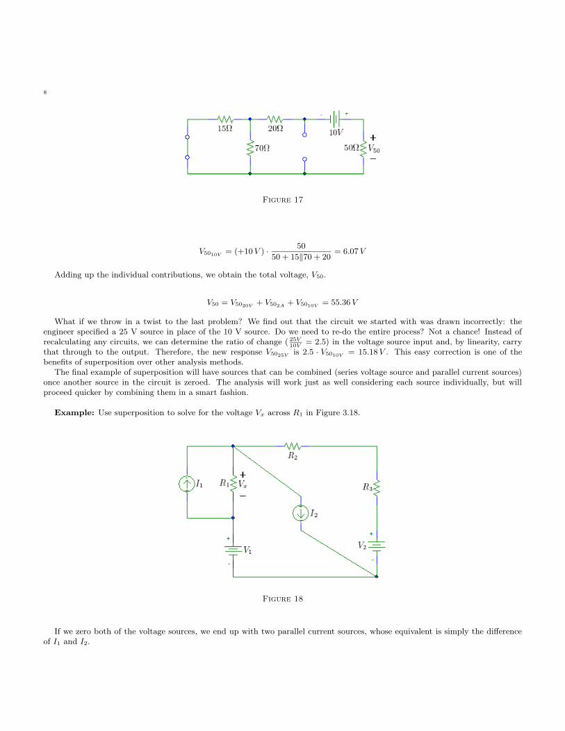
Figure 17

V5010V= (+10 V ) ·

50

50 + 15‖70 + 20= 6.07 V

Adding up the individual contributions, we obtain the total voltage, V50.

V50 = V5020V+ V502A

+ V5010V= 55.36 V

What if we throw in a twist to the last problem? We find out that the circuit we started with was drawn incorrectly: theengineer specified a 25 V source in place of the 10 V source. Do we need to re-do the entire process? Not a chance! Instead ofrecalculating any circuits, we can determine the ratio of change ( 25V

10V= 2.5) in the voltage source input and, by linearity, carry

that through to the output. Therefore, the new response V5025Vis 2.5 · V5010V

= 15.18 V . This easy correction is one of thebenefits of superposition over other analysis methods.

The final example of superposition will have sources that can be combined (series voltage source and parallel current sources)once another source in the circuit is zeroed. The analysis will work just as well considering each source individually, but willproceed quicker by combining them in a smart fashion.

Example: Use superposition to solve for the voltage Vx across R1 in Figure 3.18.

Figure 18

If we zero both of the voltage sources, we end up with two parallel current sources, whose equivalent is simply the differenceof I1 and I2.

9

Figure 19

Likewise, when we zero both current sources, there is a single series loop containing two voltage sources.

Figure 20

By solving the circuits in Figures 3.19 and 3.20, we reduce the workload by nearly half (two circuits instead of four). Theoverall solution is:

Vx = VxI1−I2+ VxV2−V1

= (I1 − I2) · R1‖(R2 + R3) + (V2 − V1) ·R1

R1 + R2 + R3

To conclude the section, we state the general steps necessary to solve any circuit using superposition.

1. Establish the unknown’s voltage polarity or current direction (and keep consistent throughout the analysis).2. Redraw a circuit containing k voltage or current sources into k seperate circuits where only one source is active and all

others are zeroed. Remember: zero voltage sources are short circuits while zero current sources are open circuits.3. Solve for each sources’ contribution to the overall voltage or current using Ohm’s law and dividers as appropriate.4. Add the individual contributions to obtain the desired overall quantity.

A final comment on superposition: nearly every mainstream textbook on linear circuit analysis has a disclaimer that you cannotperform superposition on circuits containing controlled sources. This notion is false!1 We will routinely use superposition whenconsidering operational amplifier and transistor circuits, treating all controlled sources as independent (non-controlled sources)and rectifying the algebra later.

Other Linear techniques

Another consequence of circuits as linear systems is that we may write systems of equations and employ linear algebra to solve.

The equations will ultimately fit into Ohm’s law: we will re-write the traditional matrix equation [A]~x = ~b as either ~V = [Z]~I or

[Y ]~V = ~I, where [Z] is the matrix of impedances ([Y ] is the matrix of admittances) relating voltages to currents. The same basicrules from linear algebra apply: the matrix [Z] or [Y ] must be invertible (have a non-zero determinant) for there to be a solution,

1Leach: something

10

and you need as many independent equations as unknowns to fully solve.

§3.3: Node-Voltage Analysis

Node-voltage analysis expands Kirchoff’s current law to write equations at each node in a circuit, and then solve with linearalgebra (ideally using a computer). We also draw on the fact that voltage is a conservative field, whose potentials can be takenrelative to an arbitrary reference point; thus we will be allowed to define a ground node as 0 V (typically, we choose the nodethat has the most connections to other nodes in an attempt to simplify the equations).

Consider the first circuit that we analyzed using superposition.

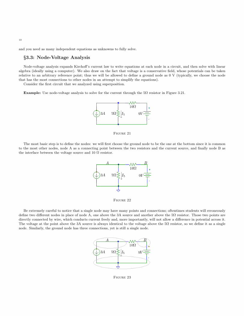
Example: Use node-voltage analysis to solve for the current through the 5Ω resistor in Figure 3.21.

Figure 21

The most basic step is to define the nodes: we will first choose the ground node to be the one at the bottom since it is commonto the most other nodes, node A as a connecting point between the two resistors and the current source, and finally node B asthe interface between the voltage source and 10 Ω resistor.

Figure 22

Be extremely careful to notice that a single node may have many points and connections; oftentimes students will erroneouslydefine two different nodes in place of node A, one above the 3A source and another above the 5Ω resistor. Those two points aredirectly connected by wire, which conducts current freely and, more importantly, will not allow a difference in potential across it.The voltage at the point above the 3A source is always identical to the voltage above the 5Ω resistor, so we define it as a singlenode. Similarly, the ground node has three connections, yet is still a single node.

Figure 23

11

We will write two independent equations relating the unknown voltages at nodes A and B to the input sources and passivecomponents. First, writing a KCL equation at node A (assume all currents to be leaving the node), we obtain:

3A +VA − 0

5Ω+

VA − VB

10Ω= 0

Normally, we would try to write a second equation at node B, but we find our first problem: we do not know the current intoan ideal voltage source (the potential is fixed completely independent of the current flowing through the source).

VB − VA

10Ω+ I9V = 0

I9V =???

There is a way to bypass the indeterminate nature of the current through the voltage source: simply realize that KCL worksfor arbitrary black boxes (linear) as well, and thus state that the current entering the voltage source is equal to the current leavingthe voltage source.

Figure 24

The actual name for this treatment of the voltage source is that of a supernode. Writing the new equation, we end up withanother KCL equation.

VB − VA

10Ω+

0 − VA

5Ω+ −3A = 0

Simplifying this equation shows another interesting false start to node-voltage analysis: this equation is exactly the same asthe one written at node A! Multiply both sides by a (−1) and you get the other equation. If the two equations are the same, thenthey are also linearly dependent; to solve a linear system consisting of two unknowns, you must have two independent equations(in general, the number of independent equations must equal the number of unknowns). We’ve exhausted the nodes at which towrite KCL equations, but we do know a very simple equation relating the two nodes having the voltage source between them.

VB − 0 = 9V

Thus, taking the voltage source as a fixed potential between two points, we obtain the final equation. Writing the two equationstogether, we can form a linear system of equations (i.e. a matrix) to solve.

„

15Ω

+ 110Ω

− 110Ω

1 0

«

·

„

VA

VB

«

=

„

−3A

9V

«

Notice that the elements of the matrix are simply the coefficients of the unknown node voltages. Further, you should checkthat the units of each element in the expression make sense (matrix multiplication being across a row of the matrix and down thecolumn vector of the unknowns).

Once the equations are set into a matrix, we have a slew of choices how to solve: Gaussian elimination, Cramer’s rule, orinverting the matrix. In general, you should be well versed in solving linear equations either by hand or with the aid of computationsoftware, so we will not cover those here.2 Even so, we are not quite finished. When a specific variable is requested (we asked forthe downward current in the 5Ω resistor), we must solve for that quantity in terms of the, now known, node voltages.

~V =

„

VA

VB

«

= [Y ]−1 · ~I =

„

−7V

9V

«

I5 =VA

5Ω= −1.4 A

2A great reference on linear algebra for solving linear systems of equations by hand is “Apostol: Linear Algebra”

12

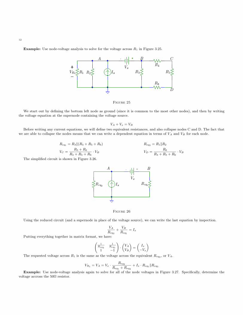
Example: Use node-voltage analysis to solve for the voltage across R1 in Figure 3.25.

Figure 25

We start out by defining the bottom left node as ground (since it is common to the most other nodes), and then by writingthe voltage equation at the supernode containing the voltage source.

VA + Vx = VB

Before writing any current equations, we will define two equivalent resistances, and also collapse nodes C and D. The fact thatwe are able to collapse the nodes means that we can write a dependent equation in terms of VA and VB for each node.

Req1 = R3‖(R4 + R5 + R6) Req2 = R1‖R2

VC =R5 + R6

R4 + R5 + R6· VB VD =

R6

R4 + R5 + R6· VB

The simplified circuit is shown in Figure 3.26.

Figure 26

Using the reduced circuit (and a supernode in place of the voltage source), we can write the last equation by inspection.

VA

Req2

+VB

Req1

= Ix

Putting everything together in matrix format, we have:

1Req2

1Req1

1 −1

!

·

„

VA

VB

«

=

„

Ix

−Vx

«

The requested voltage across R1 is the same as the voltage across the equivalent Req2 , or VA.

VR1= VA = Vx ·

Req2

Req1 + Req2

+ Ix · Req1‖Req2

Example: Use node-voltage analysis again to solve for all of the node voltages in Figure 3.27. Specifically, determine thevoltage accross the 50Ω resistor.

13

Figure 27

The first step is to write the easy equations between nodes having voltage sources between them, and then collect anyimpedances into equivalents.

VA − 0 = 20 V

VD − VC = 10 V

Since we have four unknown voltages, and so far two equations, we need to write two independent KCL equations as follows.

VB − VA

15 Ω+

VB − 0

70Ω+

VB − VC

20Ω= 0

VC − VB

20Ω+

VD − 0

50 Ω− 2 A = 0

We have applied the supernode condition in the second equation: the current leaving node C into the voltage source is thesame as the sum of the currents leaving node D. Combining the four equations into matrix format (we will now omit the units

since they cancel), we reduce the linear circuit to [Y ]~V = ~I.

0

B

B

@

1 0 0 00 0 −1 1

− 115

115

+ 170

+ 120

− 120

00 − 1

20120

150

1

C

C

A

·

0

B

B

@

VA

VB

VC

VD

1

C

C

A

=

0

B

B

@

201002

1

C

C

A

Not only does solving this system via nodal analysis result in the same node voltages that we obtained in the superpositionanalysis, but the process finds all of the voltages at once!

~V =

0

B

B

@

VA

VB

VC

VD

1

C

C

A

=

0

B

B

@

20 V

27.5 V

45.36 V

55.36 V

1

C

C

A

Trivially, we solve for the voltage across the 50Ω resistor,

V50Ω = VD = 55.36 V

Any circuit parameter that we wish to find is immediately available as a function of the node voltages. As an exercise, youshould verify the conservation of energy using the solution above (you will need to use the voltages across the 15 and 50 Ω resistorsto obtain the currents in the 20 and 10 V sources, respectively).

Example: Use node-voltage analysis to solve for the voltage across R1 in Figure 3.28.

14

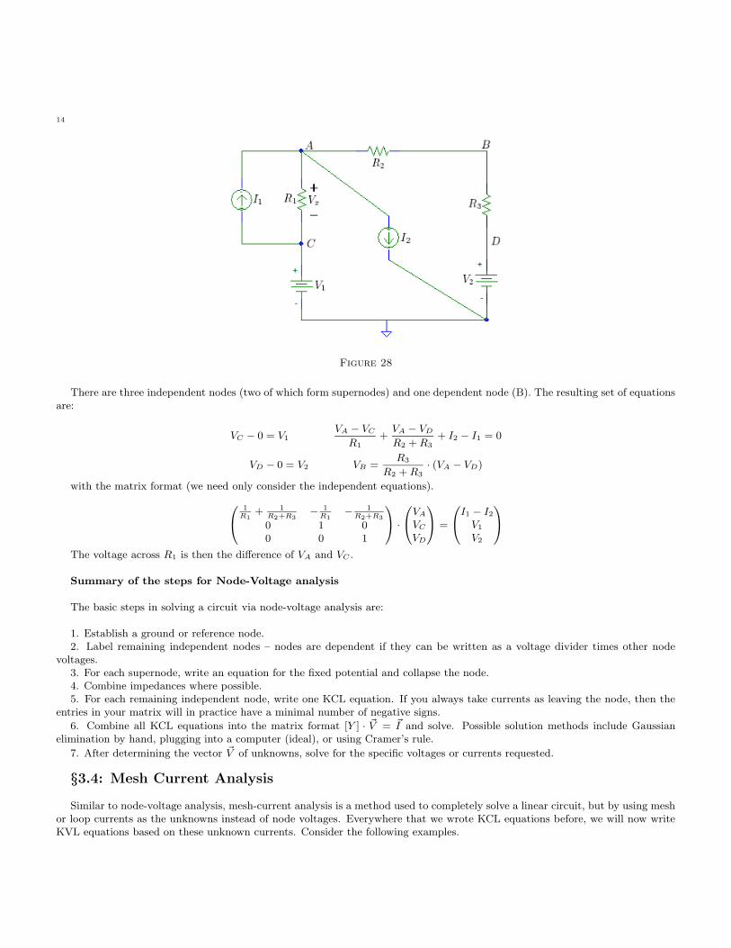
Figure 28

There are three independent nodes (two of which form supernodes) and one dependent node (B). The resulting set of equationsare:

VC − 0 = V1VA − VC

R1+

VA − VD

R2 + R3+ I2 − I1 = 0

VD − 0 = V2 VB =R3

R2 + R3· (VA − VD)

with the matrix format (we need only consider the independent equations).

0

@

1R1

+ 1R2+R3

− 1R1

− 1R2+R3

0 1 00 0 1

1

A ·

0

@

VA

VC

VD

1

A =

0

@

I1 − I2

V1

V2

1

A

The voltage across R1 is then the difference of VA and VC .

Summary of the steps for Node-Voltage analysis

The basic steps in solving a circuit via node-voltage analysis are:

1. Establish a ground or reference node.2. Label remaining independent nodes – nodes are dependent if they can be written as a voltage divider times other node

voltages.3. For each supernode, write an equation for the fixed potential and collapse the node.4. Combine impedances where possible.5. For each remaining independent node, write one KCL equation. If you always take currents as leaving the node, then the

entries in your matrix will in practice have a minimal number of negative signs.

6. Combine all KCL equations into the matrix format [Y ] · ~V = ~I and solve. Possible solution methods include Gaussianelimination by hand, plugging into a computer (ideal), or using Cramer’s rule.

7. After determining the vector ~V of unknowns, solve for the specific voltages or currents requested.

§3.4: Mesh Current Analysis

Similar to node-voltage analysis, mesh-current analysis is a method used to completely solve a linear circuit, but by using meshor loop currents as the unknowns instead of node voltages. Everywhere that we wrote KCL equations before, we will now writeKVL equations based on these unknown currents. Consider the following examples.

15

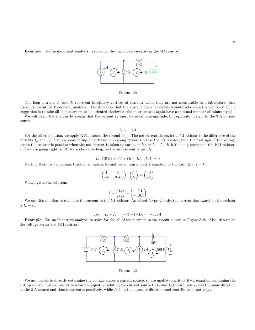
Example: Use mesh-current analysis to solve for the current downwards in the 5Ω resistor.

Figure 29

The loop currents Ia and Ib represent imaginary vortices of current: while they are not measurable in a laboratory, theyare quite useful for theoretical analysis. The direction that the current flows (clockwise/counter-clockwise) is arbitrary, but asuggestion is to take all loop currents to be oriented clockwise (the matrices will again have a minimal number of minus signs).

We will begin the analysis by seeing that the current Ia must be equal in magnitude, but opposite in sign, to the 3 A currentsource.

Ia = −3 A

For the other equation, we apply KVL around the second loop. The net current through the 5Ω resistor is the difference of thecurrents Ia and Ib; if we are considering a clockwise loop going upwards across the 5Ω resistor, then the first sign of the voltageacross the resistor is positive when the net current is taken upwards, or I5Ω = Ib − Ia. Ib is the only current in the 10Ω resistor,and we are going right to left for a clockwise loop, so the net current is just Ib

Ib · (10 Ω) + 9 V + (Ib − Ia) · (5 Ω) = 0

Putting these two equations together in matrix format, we obtain a matrix equation of the form [Z] · ~I = ~V .

„

1 0−5 10 + 5

«

·

„

Ia

Ib

«

=

„

−3−9

«

Which gives the solution:

~I =

„

Ia

Ib

«

=

„

−3A

−1.6A

«

We use this solution to calculate the current in the 5Ω resistor. As solved for previously, the current downwards in the resistoris Ia − Ib.

I5Ω = Ia − Ib = (−3) − (−1.6) = −1.4 A

Example: Use mesh-current analysis to solve for the all of the currents in the circuit shown in Figure 3.30. Also, determinethe voltage across the 50Ω resistor.

Figure 30

We are unable to directly determine the voltage across a current source, so are unable to write a KVL equation containing the2 Amp source. Instead, we write a current equation relating the current source to Ib and Ic (notice that Ic has the same directionas the 2 A source and thus contributes positively, while Ib is in the opposite direction and contributes negatively).

16

Ic − Ib = 2 A

We then write our KVL equations such that they bypass the current source (also called creating a super-mesh).

−20 + 15 · Ia + 70 · (Ia − Ib) = 0

70 · (Ib − Ia) + 20 · Ib − 10 + 50 · Ic = 0

Combining these three equations into matrix format, we obtain another set of linear equations, whose solution is the vector ofunknown mesh currents.

0

@

0 −1 115 + 70 −70 0−70 70 + 20 50

1

A ·

0

@

Ia

Ib

Ic

1

A =

0

@

22010

1

A =⇒ ~I =

0

@

−0.5A

−0.893A

1.11A

1

A

To compare this solution to our other methods, notice that V50 = 50 Ω · Ic = 55.36V just as before.

Example: Solve for the voltage across R1 using mesh-current analysis.

Figure 31

The first step is to determine how many equation we really need out of the four possible meshes: by combining the resistorsinto appropriate equivalents as before, we can reduce the number of meshes to two.

Figure 32

Req1 = R3‖(R4 + R5 + R6) Req2 = R1‖R2

Writing the two independent equations,

Ia · Req2 − Vx + Ib · Req1 = 0

Ib − Ia = Ix

we can set up the appropriate matrix equation,

„

Req2 Req1

−1 1

«

·

„

Ia

Ib

«

=

„

Vx

Ix

«

17

and finally solve.

~I =

„

Ia

Ib

«

=

Vx−Ix·Req1

Req1+Req2

Vx+Ix·Req2

Req1+Req2

!

Notice that this solution yields the same expressions as when we solved by superposition and nodal analysis.

VR1= −Ia · R1‖R2 =

Ix · Req1 − Vx

Req1 + Req2

· Req2 = Ix · Req1‖Req2 − Vx ·Req2

Req1 + Req2

Example: Use mesh-current analysis to solve for the voltage across R1 in Figure 3.33.

Figure 33

The two current equations will eliminate the left loop and combine the larger loops.

Ia = I1 Ib − Ic = I2

The remaining equation is obtained by a clockwise loop about the current source I2.

−V1 + R1 · (Ib − Ia) + (R2 + R3) · Ic + V2 = 0

Combining these equations and solving yet another linear system, we obtain the currents in each of the meshes.

0

@

1 0 00 1 −1

−R1 R1 R2 + R3

1

A ·

0

@

Ia

Ib

Ic

1

A =

0

@

I1

I2

V1 − V2

1

A =⇒ ~I =

0

B

@

I1I1R1+I2·(R2+R3)+V1−V2

R1+R2+R3

V1−V2+(I1−I2)·R1

R1+R2+R3

1

C

A

Summary of the steps for Mesh-Current analysis

The basic steps in solving a circuit via mesh-current analysis are:

1. Draw and label as many mesh currents as necessary.2. Write equations for any meshes containing current sources. Replace with super-meshes as appropriate.3. Combine impedances where possible.4. Write one independent equation for each of the remaining meshes. Solve the equations by hand, calculator, or computer.5. Determine the desired quantities using the resulting vector of current values.

Comparison of Analysis Techniques

So far, we have seen three different analysis techniques for linear circuits. Voltage and current dividers work well, but onlywhen there is one power source. Superposition reduces the analysis of complicated circuits to simplified circuits (with zero-ed

18

sources) where we can use dividers to calculate the contribution of each source to a single desired quantity. Node-voltage analysisuses KCL equations to determine all of the node voltages in a circuit, and mesh-current analysis uses KVL equations to determineall the mesh currents, but neither solves directly for specific voltages or currents. Node/mesh analyses do however provide allthe information in the circuit at once. With this information, the question becomes: how do you choose which method to use insolving a circuit?

We will explore various factors that affect which method we use: time, access to computing tools, analysis of perturbations,and desired form of outputs are just a few to consider. Strictly speaking, analysis of circuits can take the form of any combinationof these methods. One remaining way to solve linear circuits is to create circuit equivalents (containing both impedances andpower sources), reducing the circuit as much as possible before analysing.

§3.5: Equivalent Circuits

Now that we know the basic steps to analyze a circuit, what happens if we want to use the circuit in a system, especially if thatsystem changes? Common devices as seemingly simple as an alarm clock may consist of hundreds of circuit elements, so we needa modeling technique that allows us replace the large circuits by much smaller, and much easier to calculate, equivalent circuits.The two types of representations we introduce now are called Thevinin and Norton equivalents. The Thevinin equivalent of anylinear circuit is defined as a voltage source in series with a single resistance (impedance) having the same terminal characteristicsas the original circuit, while a Norton equivalent is defined by a current source in parallel with the same Thevinin resistance(impedance), still with identical terminal characteristics. Both the Thevinin and Norton equivalents could replace the originalcircuit without us being able to tell the difference from outside the circuit.

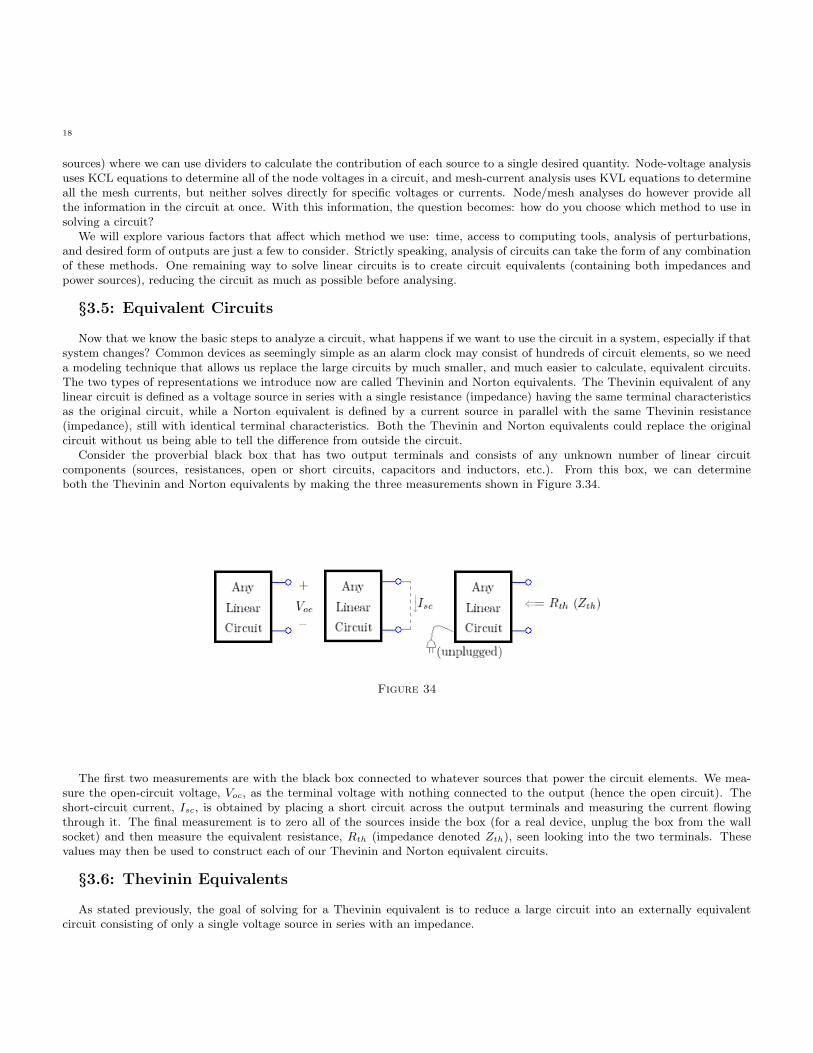
Consider the proverbial black box that has two output terminals and consists of any unknown number of linear circuitcomponents (sources, resistances, open or short circuits, capacitors and inductors, etc.). From this box, we can determineboth the Thevinin and Norton equivalents by making the three measurements shown in Figure 3.34.

Figure 34

The first two measurements are with the black box connected to whatever sources that power the circuit elements. We mea-sure the open-circuit voltage, Voc, as the terminal voltage with nothing connected to the output (hence the open circuit). Theshort-circuit current, Isc, is obtained by placing a short circuit across the output terminals and measuring the current flowingthrough it. The final measurement is to zero all of the sources inside the box (for a real device, unplug the box from the wallsocket) and then measure the equivalent resistance, Rth (impedance denoted Zth), seen looking into the two terminals. Thesevalues may then be used to construct each of our Thevinin and Norton equivalent circuits.

§3.6: Thevinin Equivalents

As stated previously, the goal of solving for a Thevinin equivalent is to reduce a large circuit into an externally equivalentcircuit consisting of only a single voltage source in series with an impedance.

19

Figure 35

The value of the voltage source is equal to the open-circuit or Thevinin voltage, Voc, and the impedance is the Thevininimpedance, Zth.

Example: Calculate the Thevinin or open-circuit voltage and the Thevinin impedance to the left of the 50 Ω resistor in Figure3.36. Verify that the equivalent circuit produces the same voltage V50 as before.

Figure 36

The first step is to designate what is inside the black box we are trying to model and what is outside the box. As designatedon the schematic, we are looking for the Thevinin equivalent to the left of the dashed line. This specifically means that the 50Ωresistor is not to be considered part of the circuit for modeling purposes, resulting in a true open circuit at the dashed lines. Tocalculate this open-circuit voltage, we may use any of the circuit analysis techniques learned previously. The 10 V source doesnot contribute any current to the rest of the circuit (due to its placement in series with an open circuit), and we are only lookingfor one specific voltage: superposition will be the best choice.

The three circuits in Figure 3.37 show the decomposition of Figure 3.36 into sub-circuits with only one source active. Wecalculate the contributions from each source to the voltage Voc and add these contributions to obtain the total Voc.

Figure 37

The trickiest of the three sub-circuits is the third one: since no current is able to flow through the open circuit, there is zerocurrent in any of the resistors. This results in a zero voltage across the resistors, whose potential is then added in series to thepotential difference of the 10V source. For similar reasons, there is no current flowing in the 20Ω resistor in the first circuit, andthus Voc is the same as the voltage across the 70Ω resistor.

20

Voc = Voc20V+ Voc2A

+ Voc10V=

70

70 + 15· (20V ) + (2A) · (20 + 15‖70)Ω + (10V ) = 91.18 V

To calculate the Thevinin resistance (impedance), we zero all of the independent sources, and solve for the equivalent impedancelooking into the two terminals. Figure 3.38 shows the circuit with all sources zeroed.

Figure 38

By inspection,

Rth = (20 + 15‖70) Ω = 32.35 Ω

Putting these two parameters together, we form a series combination of Voc and Rth and replace everything to the left of theoriginal dashed line with our new equivalent.

Figure 39

How do we check if this new “equivalent” circuit truly has the same effect as the original? Reconnecting the 50Ω resistor as aload onto the new circuit, we can calculate the voltage V50, which should be the same voltage we solved for in previous examples.

Figure 40

Using a single voltage divider,

V50 = Voc

50

50 + Rth

= 55.36 V

Now why in the world did we go through that much work to obtain the same answer as before? Consider a case where theleft side of our circuit (for which we obtained the Thevinin equivalent) is a stereo amplifier and the 50 Ω resistor is a collectionof speakers that we want to hook up. What happens if we then want to add/remove a speaker? Each of the other numericalanalyses performed would be useless once an impedance value is changed, whereas the Thevinin equivalent makes the calculationeasy in any case; simply recalculate the voltage divider at the end. Let’s try a few more examples, and then we will explore the

21

relationships between methods in more depth.

Example: Use a Thevinin equivalent circuit to solve for the current through the 5Ω resistor in Figure 3.41. Repeat thesolution with the 5Ω resistor changed to 25Ω.

Figure 41

Although smaller, this circuit is harder to conceptualize. We may redraw the circuit without the 5Ω resistor and stretch outthe nodes for better visualization.

Figure 42

Solving for Voc by superposition, and Zth by zeroing all of the sources, we obtain the values for the Thevinin equivalent.

Voc = 9V + (−3A) · 10Ω = −21V Zth = 10Ω

To calculate the voltage across a load resistor connected to the output nodes, we attach an arbitrary load, Rload, as shown inFigure 3.43, and use Ohm’s law to get the current.

Figure 43

IRload=

−21V

10Ω + Rload

For load resistors of 5Ω and 25Ω, we calculate −1.4A and −0.6A, respectively.

Some circuits simply have no easy solution with the previous techniques discussed. Thevinin and Norton equivalents providea new method that works where others fail.

Example: Consider the bridge circuit in Figure 3.44: determine the voltage across R5.

22

Figure 44

Initially, the options look rather bleak; node-voltage analysis will work, but the solution will be extremely tedious. If weremember that potentials are the same anywhere along a node, we can simplify the circuit by splitting the voltage source intotwo parallel sources of the same value, shown in Figure 3.45.

Figure 45

With identical potentials at both the top and bottom nodes, we can see that there will be no current flowing at the top of R1

and R2 or below R3 and R4. Therefore, removing the connections will not affect our analysis of the circuit.

23

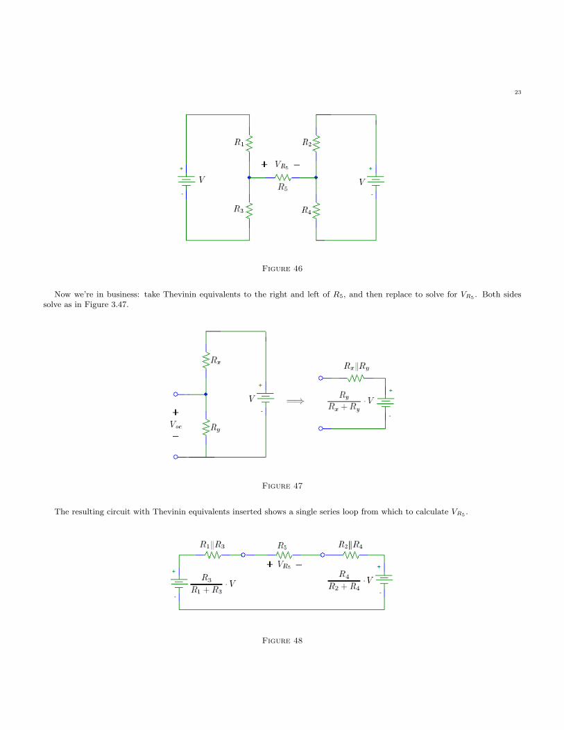
Figure 46

Now we’re in business: take Thevinin equivalents to the right and left of R5, and then replace to solve for VR5. Both sides

solve as in Figure 3.47.

Figure 47

The resulting circuit with Thevinin equivalents inserted shows a single series loop from which to calculate VR5.

Figure 48

24

VR5= V · [

R3

R1 + R3−

R4

R2 + R4] ·

R5

R1‖R3 + R5 + R2‖R4

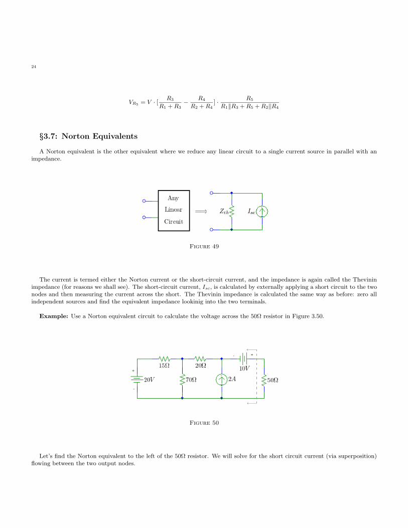
§3.7: Norton Equivalents

A Norton equivalent is the other equivalent where we reduce any linear circuit to a single current source in parallel with animpedance.

Figure 49

The current is termed either the Norton current or the short-circuit current, and the impedance is again called the Thevininimpedance (for reasons we shall see). The short-circuit current, Isc, is calculated by externally applying a short circuit to the twonodes and then measuring the current across the short. The Thevinin impedance is calculated the same way as before: zero allindependent sources and find the equivalent impedance lookinig into the two terminals.

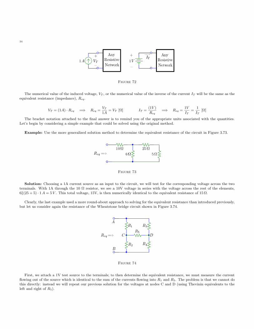
Example: Use a Norton equivalent circuit to calculate the voltage across the 50Ω resistor in Figure 3.50.

Figure 50

Let’s find the Norton equivalent to the left of the 50Ω resistor. We will solve for the short circuit current (via superposition)flowing between the two output nodes.

25

Figure 51

Some of the divider terms are tricky at first glance. In the first circuit, calculate the current into the 20Ω resistor as a dividerbetween the 20 and 70 Ω resistors; notice that the two resistors are in parallel due to the addition of the external short circuit.When calculating the equivalent impedance for the total current out of the 20V source, we consider the impedance looking rightfrom the voltage source, not left into the equivalency nodes. The second circuit is easy: current takes the path of least resistance,so all of the current goes through the short circuit. The third circuit is a single application of Ohm’s law.

Isc =70

20 + 70·

20V

(15 + 20‖70)Ω+ (2A) +

10V

(15‖70 + 20) Ω= 2.818 A

Now, we zero all of the independent sources and calculate the Thevinin impedance.

Zth = 20 + 15‖70 = 32.35Ω

Putting these two terms together, we redraw as the Norton equivalent circuit.

Figure 52

To verify our calculations, we find the voltage across the 50Ω resistor.

V50 = Isc · (Rth‖50) = 55.35 V

We again see an immediate benefit of the equivalent circuit: responses may be easily calculated for any load resistor!

Example: Calculate the Norton equivalent of the circuit shown in Figure 3.53, to the right of R1, and then us the equivalentto determine the voltage VR1

.

26

Figure 53

We reduce the circuit by taking the equivalent resistance of the right side, and begin using superposition to solve for the shortcircuit current, followed by the Thevinin impedance.

Figure 54

Solving for the Norton equivalent values:

Isc = Ix +−Vx

Req1

Zth = R2‖Req1

The resulting Norton equivalent with R1 reattached is shown in Figure 3.55.

Figure 55

We will solve for the voltage VR1in order to verify equivalency.

VR1= Isc · (Rth‖R1) = (Ix +

−V x

Req1

) · (R1‖R2‖Req1) = Ix · Req1‖R1‖R2 + (−Vx) ·R1‖R2

Req1 + R1‖R2

Example: Use a Norton equivalent circuit to solve for the current through the 5Ω resistor in Figure 3.56.

27

Figure 56

Replacing the 5Ω resistor by a short circuit in Figure 3.57, we may calculate our two parameters: Isc and Zth.

Figure 57

Isc = (−3A) +9V

10Ω= −2.1 A Zth = 10 Ω

Replacing the 5Ω resistor and calculating a current divider, we obtain the current I5.

I5 =10

10 + 5· (−2.1A) = −1.4A

Example: Use a Norton equivalent circuit to solve for the voltage across R1 in Figure 3.58.

Figure 58

Using superposition again (with a short circuit in place of R1), we obtain the expressions for short circuit current (orienteddownward) and Thevinin impedance.

Isc = I1 − I2 +V2 − V1

R2 + R3Zth = R2 + R3

28

And then finally solve for the voltage Vx.

Vx = Isc · R1‖(R2 + R3) = (I1 − I2) · R1‖(R2 + R3) + (V2 − V1) ·R1

R1 + R2 + R3

§3.8: Duality of Equivalents: Source Transformations

We have so far derived two entirely different methods for modeling a large linear circuit as a simple “equivalent;” if bothmethods produce circuits equivalent to the original, then they should also be equivalent to each other. Consider the two circuitsin Figure 3.59, which we will take to be the Thevinin and Norton equivalents of yet a third circuit, not pictured.

Figure 59

By taking the Thevinin equivalent of the Norton equivalent, and likewise taking the Norton equivalent of the Thevininequivalent, we shall find a direct relation between them.

Rth = Zth Voc = ZthIsc Isc =Voc

Zth

Thus to find both equivalent circuits, we only need to find one of the equivalents and then convert to the other. In practice,this property allows us to build in another verification step to tell us whether our analysis is correct. The easiest, and therebythe least likely to generate errors, of the three quantities (Voc, Isc, and Zth) is the equivalent impedance. As a result, the surestmethod is to calculate both Voc and Isc and then compare the ratio Voc

Iscto the calculated value of Zth.

Converting a single voltage source in series with an impedance to current source in parallel with the same impedance is calleda source transformation. This transformation can often simplify circuits dramatically; let’s again consider the circuit shown inFigure 3.60 for which we found Thevinin and Norton equivalents.

Figure 60

We still want to find the Thevinin/Norton equivalent to the left of the dashed line, but we are going to systematically performsource transformations from the far left until we have completed the equivalent. The first step will be a source transformation forthe series combination of 20 V voltage source and 15Ω resistor, shown in Figure 3.61.

29

Figure 61

Taking the Norton equivalent of just the 20V source and the 15Ω resistor, we calculate a short-circuit current Isc = 20 V15 Ω

=1.333 A, and the same 15 Ω impedance. Substituting this equivalent into the circuit, we obtain the one shown in Figure 3.62.

Figure 62

We now have the 15 and 70 Ω resistors in parallel, creating an equivalent impedance of 12.35 Ω. Reversing the source transfor-mation procedure with the new impedance (taking a Thevinin equivalent of the 12.35Ω resistor in parallel with 1.33 A source),we obtain the circuit shown in Figure 3.63.

Figure 63

Absorbing the 20 Ω resistor and taking one more source transformation, we see a new simplification: two current sources inparallel.

30

Figure 64

The two current sources add directly, so we are in effect absorbing the current source into our model. Transforming one lasttime, we obtain two series voltage sources (which add directly) and a single impedance, which is the overall Thevinin equivalentand the same equivalent circuit we obtained previously.

Figure 65

We shall consider one more example of using source transformations to reduce a circuit.

Example: Determine the Norton equivalent to the right of R1 in the circuit shown in Figure 3.66.

Figure 66

Using the same equivalent resistance, Req1 = R3‖(R4 + R5 + R6), as before and a single transformation to the right of thecurrent source, we nearly end up with the overall Norton equivalent.

31

Figure 67

Combining parallel current sources and resistances, we obtain the same equivalent as before, but in only two simple steps!

One word of caution: equivalent circuits as with any other “equivalent” are not the same thing as the original. The equivalentcircuits are wonderful mathematical tools for modeling a system, but this convenience does come at a cost: tracking variablesinternal to the collapsed circuit is nearly impossible. The equivalent circuit derived at one two-port junction will be different thananother two elements away. By no means does this realization make Thevinin or Norton equivalents unimportant–we simply seethat Norton/Thevinin equivalents are suitable for some applications and not others.

In general, the steps used to find the Thevinin and Norton equivalents of a circuit are:

1. Separate those elements that are part of the equivalent and those that are external. Clearly label the polarity of Voc andthe direction of Isc, making sure they line up with the polarity/direction of the desired equivalent.

2. Solve for Voc and Isc using any method desired: superposition, nodal or mesh analysis, etc.3. At any point, you may wish to employ a source transformation to reduce the circuit to a simpler form.4. Replace the larger circuit by its calculated equivalent and proceed with any external load calculations.

§3.9: Maximum Power Transfer

We have stated that both Thevinin and Norton equivalents can be used to model a linear circuit for use in calculating responsesdue to many loads. The most common goal in electronics is to transfer information with the least loss in the signal: in circuits,this goal translates to delivering the maximum amount of power possible to a load. How do we achieve such maximum powertransfer?

Consider a loaded Thevinin equivalent, where both the Thevinin impedance and the load are purely real (resistors), as shownin Figure 3.68.

Figure 68

The power transferred to the load is a product of its current and voltage (other forms give the same result). We may writethis power as:

Pload =Vth

Rth + Rload

·Vth · Rload

Rth + Rload

32

To maximize this power relation, we differentiate with respect to Rload, and solve for the condition on Rload to make thederivative zero.

d

dRload

Pload = 0 =⇒ Rload = Rth

We find that the maximum power transfer occurs when Rload = Rth; or, equivalently, maximum power transfer occurs whenthe load resistance to any device is equal to the Thevinin resistance of the driving circuit (for general impedances, maximumpower transfer occurs when Zload = Z∗

th).To verify this condition on Rload qualitatively, consider again the power delivered to Rload as the product of the voltage across

it and the current through it. If Rload is too small, then the voltage across it is also small, while if Rload is too large, the currentthrough both Rth and Rload will be made small. Somewhere in between we obtain the maximum of this product, as shown inFigure 3.69.

Figure 69

The value of the maximum real power that a circuit can deliver may be written using the Thevinin resistance and either theshort-circuit current or the open-circuit voltage. (Notice that for Rload = Rth, the value of both the voltage divider for the voltageacross the load and the current divider for the current through the load are equal to 1

2.)

Pmax =V 2

oc

4Rth

=I2

scRth

4We will reconsider this limit on power transfer for general impedances later on.

Example: Solve for the load resistance that maximizes the power transfer from the circuit in Figure 3.70. What is themaximum power that can be transferred?

Figure 70

Solution: To solve for the appropriate load resistance, we only need to find the Thevinin resistance of the circuit, and thenspecify the load resistance to have the same value.

Rload = Rth = 15 + 6‖30 = 20 Ω

To determine the amount of power delivered to the load, we need to calculate either the open-circuit voltage or the short-circuitcurrent. The expressions for both are shown.

33

Voc = (12 V ) ·30

30 + 6+ (1 A) · (6‖30) = 15 V

Isc =(12 V )

6 + 15‖30·

30

15 + 30+ (1 A) ·

6‖30

6‖30 + 15= 0.75 A

With these values calculated, we determine the power delivered to a 20 Ω load resistor.

P20 Ω =(15 V )2

4 · 20 Ω=

(0.75 A)2 · 20 Ω

4= 2.81 W

Example: What is the value of R in Figure 3.71, assuming that the 10 Ω load resistor was chosen for maximum power transfer?How much power is delivered?

Figure 71

To determine R, find the Thevinin resistance and set it equal to the 10 Ω to ensure maximum power transfer.

Rth = R + 2 + 0 = 10 Ω =⇒ R = 8Ω

Notice that zeroing the voltage sources also shorts out the 15Ω resistor, resulting in the zero term above. Next, to find thepower delivered, find either the open-circuit voltage or the short circuit current,

Voc = (2 V ) + (1 A) · (2 Ω) = 4 V Isc =(2 V )

2 + 8+ (1 A) ·

2

2 + 8= 0.4 A

and calculate the power.

P10 Ω =(4 V )2

4 · 10 Ω=

(0.4 A)2 · 10 Ω

4= 0.4 W

Exercise: Explain why the 15 Ω resistor in the previous circuit played no part in the analysis or solution. Consider theproperties of an ideal voltage source.

You will often hear electrical engineers speak of “impedance matching:” one of the most common errors in system design isfor subsystems to have an impedance mismatch, thereby wasting electrical power. The idea of maximum power transfer andimpedance matching drives good circuit design. We will come back to this idea in discussions of complex power and systemintegration.

§3.10: Equivalent Resistance Revisited

We have seen that some configurations of resistances (impedances), for example the bridge configuration, have no series orparallel components. To obtain the equivalent resistances of these circuits, we must try a new method besides successive paralleland series equivalents. If we use our knowledge of Thevinin and Norton equivalent circuits, we may express the equivalentresistance (impedance) as a quasi-ratio of a open-circuit voltage and short-circuit current. More exactly, we attach a 1V voltagesource or a 1A current source and test for the current or voltage, respectively.

34

Figure 72

The numerical value of the induced voltage, VT , or the numerical value of the inverse of the current IT will be the same as theequivalent resistance (impedance), Req.

VT = (1A) · Req =⇒ Req =VT

1A= VT [Ω] IT =

(1V )

Req

=⇒ Req =1V

IT

=1

IT

[Ω]

The bracket notation attached to the final answer is to remind you of the appropriate units associated with the quantities.Let’s begin by considering a simple example that could be solved using the original method.

Example: Use the more generalized solution method to determine the equivalent resistance of the circuit in Figure 3.73.

Figure 73

Solution: Choosing a 1A current source as an input to the circuit, we will test for the corresponding voltage across the twoterminals. With 1A through the 10 Ω resistor, we see a 10V voltage in series with the voltage across the rest of the elements,6‖(25 + 5) · 1 A = 5 V . This total voltage, 15V, is then numerically identical to the equivalent resistance of 15 Ω.

Clearly, the last example used a more round-about approach to solving for the equivalent resistance than introduced previously,but let us consider again the resistance of the Wheatstone bridge circuit shown in Figure 3.74.

Figure 74

First, we attach a 1V test source to the terminals; to then determine the equivalent resistance, we must measure the currentflowing out of the source which is identical to the sum of the currents flowing into R1 and R3. The problem is that we cannot dothis directly: instead we will repeat our previous solution for the voltages at nodes C and D (using Thevinin equivalents to theleft and right of R5).

35

VC = (1 V ) ·R4

R3 + R4+ (1 V ) ·

»

R2

R1 + R2−

R4

R3 + R4

–

·R5 + R3‖R4

R1‖R2 + R3‖R4 + R5

VD = (1 V ) ·R4

R3 + R4+ (1 V ) ·

»

R2

R1 + R2−

R4

R3 + R4

–

·R3‖R4

R1‖R2 + R3‖R4 + R5

Now, returning to the original circuit, we may calculate the currents down through R1 and R3,

IR1=

VA − VC

R1IR3

=VA − VD

R3

and then add them using a Kirchoff’s Current Law equation at node A to obtain the current through the voltage source andour equivalent resistance.

IT = IR1+ IR3

Req =1

IT

[Ω] = .... =R5 · (R1‖R3) + R1R3

R1 + R3 + R5+ R2‖R4

We will not waste space with massaging the algebraic formulation into the closed form; rather, we will present one numericalexample, and show that both representations work.

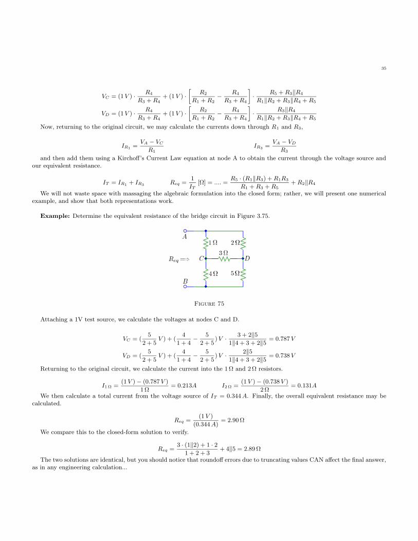
Example: Determine the equivalent resistance of the bridge circuit in Figure 3.75.

Figure 75

Attaching a 1V test source, we calculate the voltages at nodes C and D.

VC = (5

2 + 5V ) + (

4

1 + 4−

5

2 + 5) V ·

3 + 2‖5

1‖4 + 3 + 2‖5= 0.787 V

VD = (5

2 + 5V ) + (

4

1 + 4−

5

2 + 5) V ·

2‖5

1‖4 + 3 + 2‖5= 0.738 V

Returning to the original circuit, we calculate the current into the 1Ω and 2 Ω resistors.

I1 Ω =(1 V ) − (0.787 V )

1 Ω= 0.213A I2 Ω =

(1 V ) − (0.738 V )

2Ω= 0.131A

We then calculate a total current from the voltage source of IT = 0.344 A. Finally, the overall equivalent resistance may becalculated.

Req =(1 V )

(0.344 A)= 2.90 Ω

We compare this to the closed-form solution to verify.

Req =3 · (1‖2) + 1 · 2

1 + 2 + 3+ 4‖5 = 2.89 Ω

The two solutions are identical, but you should notice that roundoff errors due to truncating values CAN affect the final answer,as in any engineering calculation...

36

Exercise: In many power systems, bridge circuit are used on a regular basis; explain how you would modify the previousanalysis for two bridge circuits in parallel (hint: think about the step where KCL is applied)?

Delta-Wye Transforms

To conclude our discussion on equivalent resistances (impedances), we state two well-known, but rarely used, results forconverting to and from the ∆ and Y configurations of generic impedances shown in Figure 3.76. We have derived all of theanalysis to come up with these results in previous examples, but have omitted the algebraic mess.

Figure 76

ZA =Z1Z3

Z1 + Z2 + Z3Z1 =

ZAZB + ZAZC + ZBZC

ZB

ZB =Z2Z3

Z1 + Z2 + Z3⇐⇒ Z2 =

ZAZB + ZAZC + ZBZC

ZA

ZC =Z1Z2

Z1 + Z2 + Z3Z3 =

ZAZB + ZAZC + ZBZC

ZC

§3.11: Linear Circuit Examples

Without a doubt, the prerequisite to truly understanding linear circuits is practice. The individual concepts are in practiceextraordinarily simple: Ohm’s law is just V = I R, power is P = I V , and Kirchoff’s laws are simple sums. Putting the conceptstogether to solve any particular circuit is a more difficult task. We complete this rather long discourse on solving linear circuitsby giving two more basic circuits and solving with each of the methods presented.

The first set of examples uses a large, but relatively simple, linear circuit shown in Figure 3.77. We will see that fundamentalconcepts like equivalent resistances as well as voltage and current dividers are used over and over.

37

Figure 77

Example: To start out, solve for the equivalent voltage Vx across the 6 Ω resistor.

We solve by zeroing all but one source at a time, calculating the contribution of each source to the voltage Vxi , and finallyadding the contributions to determine the total voltage Vx. Figure 3.78 shows each of the four circuits with only one sourceactivated.

Figure 78

Each of the individual circuits reduces to a voltage or current divider, adding up to obtain the voltage Vx.

Vx = Vx0.5 A+ Vx15 V

+ Vx1 A+ Vx22 V

= (0.5 A) ·12

12 + (8 + 6‖50)· (6‖50 Ω) + (15 V ) ·

6‖(8 + 12)

6‖(8 + 12) + 50

+ (−1 A) ·8 + 12

8 + 12 + 6‖50· (6‖50 Ω) + (22 V ) ·

6‖50

6‖50 + 8 + 12

= (1.268 V ) + (1.268 V ) + (−4.225 V ) + (4.648 V ) = 2.958 V

Example: Next, setup and solve the necessary node-voltage equations to obtain Vx.

The redrawn circuit, with all nodes labeled, is shown in Figure 3.79.

Figure 79

38

We write the four equations necessary to solve,

VC − VB = 22 VVA

12+

VA − VB

8= 0.5 A VD = 15 V

VB − VA

8+ (1 A) +

VC

6+

VC − VD

50= 0

and then compute the four node voltages. You should readily notice that the desired unknown, VX , is the same as node voltageVC .

VA = −9.028 V VB = −19.046 V VC = Vx = 2.954 V VD = 15 V

We see that the node voltage VC is 2.954 V, as compared to the 2.958 V found previously (identical within roundoff).

Example: Now, setup and solve the necessary mesh-current equations to solve for Vx.

The redrawn circuit, with all meshes labeled, is shown in Figure 3.80.

Figure 80

Writing the equations for the four meshes,

I1 = 0.5 A (I2 − I1) · (12 Ω) + I2 · (8 Ω) − 22 V + (I3 − I4) · (6 Ω) = 0

I2 − I3 = 1 A (I4 − I3) · (6 Ω) + I4 · (50 Ω) + (15 V ) = 0

and solving to obtain Vx

I1 = 0.5 A I2 = 1.2521 A I3 = 0.2521 A I4 = −0.2408 A

Vx = (I3 − I4) · (6 Ω) = 2.597 V

Example: Next, let’s find Vx using a Thevinin equivalent. To do so, we remove the 6 Ω resistor from the circuit and proceedto find the open circuit voltage (via superposition) and the Thevinin equivalent resistance as shown in Figure 3.81.

Figure 81

The open circuit voltage is obtained by superposition,

Voc = (0.5 A) · [12‖(8 + 50) Ω] ·50

8 + 50+ (−1 A) · [(8 + 12)‖50 Ω] + (22 V ) ·

50

50 + (12 + 8)+ (15 V ) ·

(8 + 12)

50 + (8 + 12)

= (4.286 V ) + (−14.286 V ) + (15.714 V ) + (4.286 V )

= 10 V

and the equivalent resistance is calculated by first zeroing all the sources and then finding the equivalent.

39

Zth = 50‖(8 + 12) = 14.286 Ω

The final calculation is to use a voltage divider for the voltage Vx across the replaced 6 Ω resistor.

Vx = Voc ·6

Zth + 6= (10 V ) ·

6

14.286 + 6= 2.958 V

Example: One more method available is to use the Norton equivalent circuit. Find the Norton equiavlent and then use Ohm’slaw to determine the voltage Vx.

Once again, we remove the 6 Ω resistor, but this time attach a short circuit in its place as shown in Figure 3.82. Care hasbeen taken to make sure that the positive direction of Isc corresponds to the proper polarity for Vx.

Figure 82

Using superposition one last time, we solve for the short circuit current,

Isc = (0.5 A) ·12

8 + 12+ (−1 A) +

(22 V )

(8 + 12) Ω+

(15 V )

50 Ω

= (0.3 A) + (−1 A) + (1.1 A) + (0.3 A)

= 0.7 A

and then solve for the voltage across the parallel equivalent of Thevinin resistance (same as before) and the 6 Ω resistor.

Vx = Isc · (Zth‖6) = (0.7 A) · (14.286‖6 Ω) = 2.958 V

Example: The final method to solve this circuit is to use source transformations. Taking the original circuit, we iterativelyreduce the circuit to either a Thevinin or Norton equivalent. Performing one source transformation on both the left and the rightside of the circuit, we reduce it to the one shown in Figure 3.83.

Figure 83

Three more iterations shown in Figures 3.84, 3.85, and 3.86 give the same Norton equivalent as solve for previously.

40

Figure 84

Figure 85

Figure 86

With the final step, we calculate the voltage Vx.

Vx = (0.7 A) · (14.286‖6 Ω) = 2.958 V

Exercise: What are the benefits/limitations for each of the methods presented in this section?

We will repeat the full analysis for a second circuit that contains a number of transparent tricks. The analysis for the variousmethods will actually be less involved, but require you to see fundamental simplification.

Example: Solve for the voltage Vx across the 15Ω resistor in Figure 3.87 using each of the circuit methods.

Figure 87

41

Before we begin the analyses, we should take a moment to guesstimate what the overall characteristics will be:

1. The circuit has four independent sources, so superposition will require solving four separate circuits.2. The circuit has 6 independent sources, but three voltage sources that will make for simple node equations.3. The circuit has 5 independent meshes, yet only one current source for a simple equation.4. The 3V, 12V, and 1A will contribute to current flowing upwards in the 15Ω resistor (creating a negative contribution to

Vx), while the 22V source will contribute to a downward current and a positive Vx.5. The 4Ω resistor in series with the current source and the 8Ω resistor in parallel with the 3V voltage source will not affect

any of the other circuit variables; the voltage across a current source and the current through a voltage source are indeterminate.Any value of resistance can be used for these two without changing other circuit variables.

6. Although non-trivial to determine, by far the easiest method to solve this circuit would be source transformations in com-bination with superposition.

We will comment on these observations in more details as we proceed.

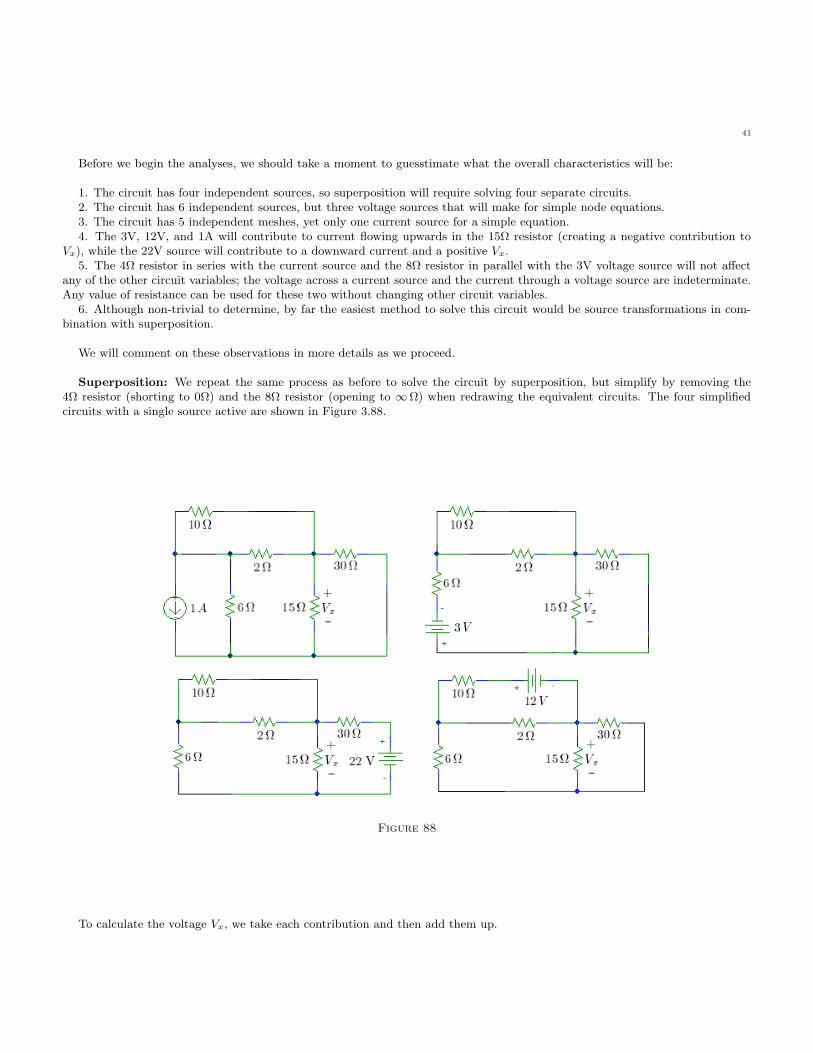
Superposition: We repeat the same process as before to solve the circuit by superposition, but simplify by removing the4Ω resistor (shorting to 0Ω) and the 8Ω resistor (opening to ∞Ω) when redrawing the equivalent circuits. The four simplifiedcircuits with a single source active are shown in Figure 3.88.

Figure 88

To calculate the voltage Vx, we take each contribution and then add them up.

42

Vx1 A= (−1 A) ·

6

6 + 10‖2 + 15‖30· (15‖30 Ω) = −3.396 V

Vx3 V= (−3 V ) ·

15‖30

15‖30 + 10‖2 + 6= −1.698 V

Vx22 V= (22 V ) ·

15‖(6 + 2‖10)

30 + 15‖(6 + 2‖10)= 3.182 V

Vx12 V= (−12 V ) ·

2‖(6 + 15‖30)

10 + 2‖(6 + 15‖30)·

15‖30

6 + 15‖30= −1.132 V

Vx = Vx1 A+ Vx3 V

+ Vx22 V+ Vx12 V

= −3.04 V

Node-Voltage Analysis: We label the nodes as shown in Figure 3.89, choosing the bottom node as ground.

Figure 89

We have left the 4Ω and 8Ω resistors in the circuit, but can quickly show that they do not affect the remainder of the circuit.The current through the 4Ω resistor is the same as the 1A source

VA − VB

4 Ω+ (1 A) = 0

while the potential difference between node E and ground is just the voltage source.

VE − 0 = (−3 V )

Changing the values of these two resistors will change either the current through (the 8Ω) or the voltage across (the 4Ω) theresistors. Writing the equations to solve for the node voltages (taking all currents leaving the nodes),

VE − 0 = (−3 V ) VC − VD = (12 V ) VF − 0 = (22 V )

(1 A) +VB − VE

6+

VB − VD

2+

VB − VC

10= 0

VD − VB

2+

VC − VB

10+

VD − 0

15+

VD − VF

30= 0

Solving 5 equations simultaneously is a pain, but the results are identical.

VA = −6.77 V VB = −2.77 V VC = 8.96 V VD = −3.04 V VE = −3 V

Vx = VD = −3.04 V

Mesh Current Analysis: First, we label the meshes as shown in Figure 3.90,

43

Figure 90

Disregarding the 8Ω resistor, we end up with four meshes, resulting in the four equations:

I1 = −(1 A) (I2 − I3) · 2 + I2 · 10 + (12 V ) = 0

(3 V ) + (I3 − I1) · 6 + (I3 − I2) · 2 + (I3 − I4) · 15 = 0 (I4 − I3) · 15 + I4 · 30 + (22 V ) = 0

Solving these equations, we obtain the four mesh currents,

I1 = −1 A I2 = −1.173 A I3 = −1.038 A I4 = −0.835 A

and the overall solution for Vx.

Vx = (I3 − I4) · (15 Ω) = −3.044 V

Thevinin and Norton Equivalents

Now we will repeat the solution for the voltage Vx using both Thevinin and Norton equivalent circuits; since the two methodsare so close to one another, we will solve them together. We first remove the 15Ω resistor from the circuit and solve for the opencircuit voltage, Voc, across the terminals using superposition.

Figure 91

The solution of Voc in this circuit is identical to the analysis of the original circuit with the 15Ω resistor increased to ∞Ω, oran open circuit. To show this modification in a little more detail, first take the previous expression for Vx using superpositionand including the 15Ω resistor (which we call V ′

oc).

44

V′

oc1 A= (−1 A) ·

6

6 + 10‖2 + 15‖30· (15‖30 Ω) = −3.396 V

V′

oc3 V= (−3 V ) ·

15‖30

15‖30 + 10‖2 + 6= −1.698 V

V′

oc22 V= (22 V ) ·

15‖(6 + 2‖10)

30 + 15‖(6 + 2‖10)= 3.182 V

V′

oc12 V= (−12 V ) ·

2‖(6 + 15‖30)

10 + 2‖(6 + 15‖30)·

15‖30

6 + 15‖30= −1.132 V

Now we replace each 15Ω term with ∞Ω to obtain Voc from V ′

oc. The equivalent resistance of an open circuit (∞Ω) in serieswith any finite resistor is the open circuit, in parallel with any finite resistor is just the resistor.

Voc1 A= (−1 A) ·

6

6 + 10‖2 + ∞‖30· (∞‖30 Ω) = (−1 A) ·

6

6 + 10‖2 + 30· (30 Ω) = −4.779 V

Voc3 V= (−3 V ) ·

∞‖30

∞‖30 + 10‖2 + 6= (−3 V ) ·

30

30 + 10‖2 + 6= −2.389 V

Voc22 V= (22 V ) ·

∞‖(6 + 2‖10)

30 + ∞‖(6 + 2‖10)= (22 V ) ·

(6 + 2‖10)

30 + (6 + 2‖10)= 4.479 V

Voc12 V= (−12 V ) ·

2‖(6 + ∞‖30)

10 + 2‖(6 + ∞‖30)·

∞‖30

6 + ∞‖30= (−12 V ) ·

2‖(6 + 30)

10 + 2‖(6 + 30)·

30

6 + 30= −1.593 V

Voc = Voc1 A+ Voc3 V

+ Voc22 V+ Voc12 V

= −4.282 V

Before having the answer for Vx, we need to determine the Thevinin resistance as seen from the two terminals with all sourceszeroed: looking right, we see a 30Ω resistor and to the left, we see 6+10‖2 Ω (the 4Ω is swamped by the open circuit of the zeroedcurrent source and the 8Ω resistor is killed by the zeroed 3V voltage source).

Rth = 30‖(6 + 10‖2) = 6.106 Ω

Finally, we determine the voltage Vx as a voltage divider with the Thevinin equivalent circuit.

Vx = Voc ·15

Rth + 15= (−4.282 V ) ·

15

6.106 + 15= −3.043 V

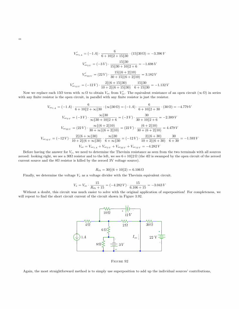
Without a doubt, this circuit was much easier to solve with the original application of superposition! For completeness, wewill repeat to find the short circuit current of the circuit shown in Figure 3.92.

Figure 92

Again, the most straightforward method is to simply use superposition to add up the individual sources’ contributions,

45

Isc = (−1 A) ·6

6 + 10‖2+

−12 V

10 + 2‖6·

2

2 + 6+

−3 V

2‖10 + 6+

22 V

30

= (−0.783 A) + (−0.261 A) + (−0.391 A) + (0.733 A)

= −0.702 A

and then apply Ohm’s law to determine the voltage Vx across the parallel combination of same Rth calculated before and thereplaced 15Ω resistor.

Vx = Isc · (Rth‖15) = (−0.702 A) · (6.106‖15 Ω) = −3.046 V

Question: Why can you not modify the superposition solution for Vx to solve for Isc?3 One hint is to consider the voltageacross a short circuit.

We found that the Norton equivalent method requires roughly the same amount of work as the original superposition solution.After working many, many, of these circuits, you will begin to see how the methods can be intermixed for quicker solutions. Ourlast example will be a hybrid method of source transformations (single-stage Thevinin or Norton equivalent) and superposition.

Hybrid Source Transformations and Superposition

First of all, take another look at the original circuit.

Figure 93

As previously discussed, the 4Ω and 8Ω resistors do not affect the rest of the circuit, so we throw them away (shorting the 4Ωand opening the 8Ω). We then notice that we have three instances of single voltage sources in series with singular resistances; weperform a source transformation on each of these terms simultaneously, obtaining the circuit in Figure 3.94.

Figure 94

3Although practically useless, you may divide the entire expression for Vx as derived using superposition by the 15Ω resistor and then take thelimit of the entire expression as the 15Ω → 0Ω, but will be forced to use L’Hopital’s rule and many, many extra steps.

46

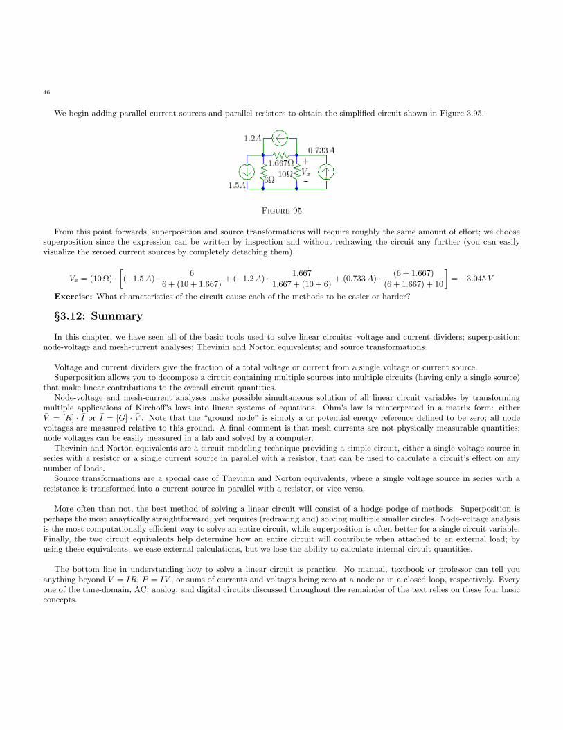
We begin adding parallel current sources and parallel resistors to obtain the simplified circuit shown in Figure 3.95.

Figure 95

From this point forwards, superposition and source transformations will require roughly the same amount of effort; we choosesuperposition since the expression can be written by inspection and without redrawing the circuit any further (you can easilyvisualize the zeroed current sources by completely detaching them).

Vx = (10 Ω) ·

»

(−1.5 A) ·6

6 + (10 + 1.667)+ (−1.2 A) ·

1.667

1.667 + (10 + 6)+ (0.733 A) ·

(6 + 1.667)

(6 + 1.667) + 10

–

= −3.045 V

Exercise: What characteristics of the circuit cause each of the methods to be easier or harder?

§3.12: Summary

In this chapter, we have seen all of the basic tools used to solve linear circuits: voltage and current dividers; superposition;node-voltage and mesh-current analyses; Thevinin and Norton equivalents; and source transformations.

Voltage and current dividers give the fraction of a total voltage or current from a single voltage or current source.Superposition allows you to decompose a circuit containing multiple sources into multiple circuits (having only a single source)

that make linear contributions to the overall circuit quantities.Node-voltage and mesh-current analyses make possible simultaneous solution of all linear circuit variables by transforming

multiple applications of Kirchoff’s laws into linear systems of equations. Ohm’s law is reinterpreted in a matrix form: eitherV = [R] · I or I = [G] · V . Note that the “ground node” is simply a or potential energy reference defined to be zero; all nodevoltages are measured relative to this ground. A final comment is that mesh currents are not physically measurable quantities;node voltages can be easily measured in a lab and solved by a computer.

Thevinin and Norton equivalents are a circuit modeling technique providing a simple circuit, either a single voltage source inseries with a resistor or a single current source in parallel with a resistor, that can be used to calculate a circuit’s effect on anynumber of loads.

Source transformations are a special case of Thevinin and Norton equivalents, where a single voltage source in series with aresistance is transformed into a current source in parallel with a resistor, or vice versa.

More often than not, the best method of solving a linear circuit will consist of a hodge podge of methods. Superposition isperhaps the most anaytically straightforward, yet requires (redrawing and) solving multiple smaller circles. Node-voltage analysisis the most computationally efficient way to solve an entire circuit, while superposition is often better for a single circuit variable.Finally, the two circuit equivalents help determine how an entire circuit will contribute when attached to an external load; byusing these equivalents, we ease external calculations, but we lose the ability to calculate internal circuit quantities.

The bottom line in understanding how to solve a linear circuit is practice. No manual, textbook or professor can tell youanything beyond V = IR, P = IV , or sums of currents and voltages being zero at a node or in a closed loop, respectively. Everyone of the time-domain, AC, analog, and digital circuits discussed throughout the remainder of the text relies on these four basicconcepts.

47

Problem 3.1 What is the Thevinin equivalent of a voltage source in parallel with a resistor? Why can you not find a Nortonequivalent?

Problem 3.2 What is the Norton equivalent of a current source in series with a resistor? Why can you not find a Thevininequivalent?

Problem 3.3: For the linear circuit shown in Figure 3.96, determine the voltage across the two output terminals.

Figure 96

Problem 3.4: For the linear circuit shown in Figure 3.97,(a) Use superposition to determine the voltage Vx.(b) Solve for Vx using node-voltage analysis.(c) Solve for Vx using mesh-current analysis.

Figure 97

Problem 3.5: For the linear circuit shown in Figure 3.98,(a) Use superposition to determine the voltage Vx.(b) Solve for Vx using node-voltage analysis.(c) Solve for Vx using mesh-current analysis.(d) Solve for Vx using the Thevinin equivalent (first remove the 84kΩ resistor).(e) Solve for Vx using the Norton equivalent (first remove the 84kΩ resistor).(f) Solve for Vx using source transformations.

Figure 98

Problem 3.6: For the linear circuit shown in Figure 3.99,

48

(a) Use superposition to determine the current Ix.(b) Solve for Ix using node-voltage analysis.(c) Solve for Ix using mesh-current analysis.(d) Solve for Ix using the Thevinin equivalent (first remove the 11kΩ resistor).(e) Solve for Ix using the Norton equivalent (first remove the 11kΩ resistor).(f) Solve for Ix using source transformations.

Figure 99

Problem 3.7: For the linear circuit shown in Figure 3.100,(a) Use superposition to determine the current Ix.(b) Solve for Ix using node-voltage analysis.(c) Solve for Ix using mesh-current analysis.(d) Solve for Ix using the Thevinin equivalent (first remove the 93kΩ resistor).(e) Solve for Ix using the Norton equivalent (first remove the 93kΩ resistor).(f) Solve for Ix using source transformations.

Figure 100

Problem 3.8: For the linear circuit shown in Figure 3.101,(a) Use superposition to determine the current Vx.(b) Solve for Vx using node-voltage analysis.(c) Solve for Vx using mesh-current analysis.(d) Solve for Vx using the Thevinin equivalent (first remove the 55kΩ resistor).(e) Solve for Vx using the Norton equivalent (first remove the 55kΩ resistor).

Figure 101

49


Figure 102

Problem 3.10: For the linear circuit shown in Figure 3.103,(a) Use superposition to determine the voltage Vx.(b) Solve for Vx using node-voltage analysis.(c) Solve for Vx using mesh-current analysis.(d) Solve for Vx using the Thevinin equivalent (first remove the 43kΩ resistor).(e) Solve for Vx using the Norton equivalent (first remove the 43kΩ resistor).

Figure 103

Problem 3.11: For the linear circuit shown in Figure 3.104,(a) Solve for Ix using node-voltage analysis.(b) Solve for Ix using mesh-current analysis.(c) Solve for Ix using the Thevinin equivalents.(d) Solve for Ix using the Norton equivalents.

Figure 104

50

Problem 3.12: For the linear circuit shown in Figure 3.105,(a) Use superposition to determine the voltage Vx.(b) Solve for Vx using node-voltage analysis.(c) Solve for Vx using mesh-current analysis.(d) Solve for Vx using the Thevinin equivalent.(e) Solve for Vx using the Norton equivalent.(f) Solve for Vx using source transformations.

Figure 105


Figure 106


51

Figure 107


Figure 108

Problem 3.16: For the circuit shown in Figure 3.109, the unknown circuit element in the middle is nonlinear and thatVx = 2 · I2 where I is the current flowing through the device. Show that superposition is no longer a valid method for thenonlinear element.

Figure 109


52

Figure 110


Figure 111

Problem 3.19: For the linear circuit shown in Figure 3.112,(a) Use superposition to determine the voltage Vx and the current Ix.(b) Solve for Vx and Ix using node-voltage analysis.(c) Solve for Vx and Ix using mesh-current analysis.(d) Solve for Vx using the Thevinin equivalent (first remove the 98kΩ resistor).(e) Solve for Ix using the Norton equivalent (first remove the 31V voltage source).

Figure 112

Problem 3.20: For the linear circuit shown in Figure 3.113,(a) Use superposition to determine the voltage Vx and the current Ix.(b) Solve for Vx and Ix using node-voltage analysis.(c) Solve for Vx and Ix using mesh-current analysis.(d) Solve for Vx using the Thevinin equivalent (first remove the 25kΩ resistor).(e) Solve for Ix using the Norton equivalent (first remove the 88kΩ resistor).

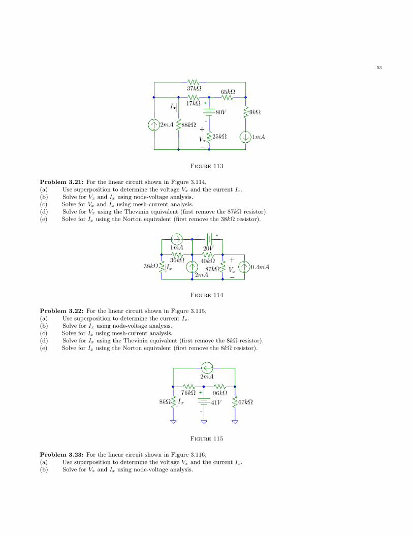
53

Figure 113


Figure 114

Problem 3.22: For the linear circuit shown in Figure 3.115,(a) Use superposition to determine the current Ix.(b) Solve for Ix using node-voltage analysis.(c) Solve for Ix using mesh-current analysis.(d) Solve for Ix using the Thevinin equivalent (first remove the 8kΩ resistor).(e) Solve for Ix using the Norton equivalent (first remove the 8kΩ resistor).

Figure 115

Problem 3.23: For the linear circuit shown in Figure 3.116,(a) Use superposition to determine the voltage Vx and the current Ix.(b) Solve for Vx and Ix using node-voltage analysis.

54

(c) Solve for Vx and Ix using mesh-current analysis.(d) Solve for Vx using the Thevinin equivalent (first remove the current source).(e) Solve for Ix using the Norton equivalent (first remove the 29kΩ resistor).

Figure 116


Figure 117

Problem 3.25: For the linear circuit shown in Figure 3.118,(a) Use superposition to determine the voltage Vx and the current Ix.(b) Solve for Vx and Ix using node-voltage analysis.(c) Solve for Vx and Ix using mesh-current analysis.(d) Solve for Vx using the Thevinin equivalent (first remove the 12kΩ resistor).(e) Solve for Ix using the Norton equivalent (first remove the 6kΩ resistor).(f) Solve for Vx and Ix using source transformations.

Figure 118

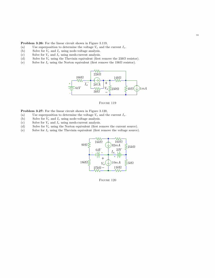
55


Figure 119

Problem 3.27: For the linear circuit shown in Figure 3.120,(a) Use superposition to determine the voltage Vx and the current Ix.(b) Solve for Vx and Ix using node-voltage analysis.(c) Solve for Vx and Ix using mesh-current analysis.(d) Solve for Vx using the Norton equivalent (first remove the current source).(e) Solve for Ix using the Thevinin equivalent (first remove the voltage source).

Figure 120

3: linear circuit analysis - hamblen.ece.gatech.eduhamblen.ece.gatech.edu/3710/ch3.pdf · x3:...

Documents