2

3

RAJAJI SYMPOSIUM

Festschrift on the occasion of

the 65th birthday of

G. Rajasekaran

22nd February 2001

Editors:

D. Indumathi, M.V.N. Murthy and R. Parthasarathy

institute of mathematical sciences report 119

FOREWORD

Professor G. Rajasekaran, or simply Rajaji to his many students and ad-mirers, completed sixty five years on 22 February 2001. His active careeras a theoretical physicist spans more than four decades so far. His career ismarked by the breadth of his research interests, clarity of thought and ex-pression, insight into subtleties and elegant exposition of these as evidencedin his research publications and conference talks. These have earned him ahighly respectable place in the community of theoretical and experimentalphysicists.

When the organising committee of the Rajaji Symposium decided to holda one-day Symposium in his honour, the response from the community oftheoretical physicists was not only spontaneous but also overwhelming. Manyof his students, collaborators and colleagues gathered on 22 February 2001to pay their tributes to him and presented contributions. This is the subjectmatter of this imsc report.

Rajaji’s research work covers a wide range, starting from hyper-nuclei,S-matrix theory, quantum field theory (in particular gauge theories), highenergy physics phenomenology, neutrino physics, gravity and quantum statis-tics. He has delivered individual and series of lectures on his work in all lead-ing research centres in India and abroad. His lectures have inspired beginnersto embark upon their research career and often helped experts to explore newstreams of thought. As an example, mention must be made of his lectures ongauge theory, delivered at the Saha Institute of Nuclear Physics, Calcutta,which emphasised the importance of gauge theories in particle physics asearly as ... This was an year before the proof of renormalisability establishedthe electroweak theory as one of the corner-stones of particle physics. Withsimilar insight, of late, he has been enthusiastically supporting the idea of anIndia-based Neutrino Observatory.

“Age cannot wither him, nor custom stale his infinite variety” of researchinterests.

The Organising Committee is thankful to the Director of the Instituteof Mathematical Sciences for his active support in conducting the one-daysymposium in Rajaji’s honour. The editors of this report also thank him forhis enthusiastic support in bringing out the proceedings in the form of animsc report.

The Editors.

Contents

1 About Rajaji 3

2 Inaugural Address 5

3 1968-1973: Some Reminiscences 9

4 Composite Fields and Fermion Masses 17

5 Proof of absence of spooky action 23

6 Are Accelerators Needed for 31

7 Ortho and Para Supersymmetric 35

8 Fock Spaces and Quantum Statistics 41

9 How do we know the charges of quarks? 49

10 Overview of semi-inclusive reactions 55

11 ΛPhys = 0 in Kaluza-Klein Formalism 61

12 Quantum Groups, q-Dynamics and Rajaji 73

13 Geometric description of Hamiltonian Chaos 81

14 Quantum dynamics of superposed 89

15 Felicitations 101

16 Rajaji’s Research Interests and Publications 107

2 CONTENTS

Chapter 1

About Rajaji

Rajaji was born on 21 February 1936 at Kamudi in Ramanathapuram district of Tamil Nadu.He had his early education in Kamudi and then in Madurai and went on to study in MadrasChristian College from where he obtained B.Sc.(Honours) with top honours.

He later joined the Training School of Atomic Energy Establishment in 1957. Afterspending three years at the training school and TIFR, he went on to do his Ph.D at theUnivesity of Chicago under the supervison of Professor Richard Dalitz.

On his return to India Rajaji spent many years at the Tata Institute of FundamentalResearch in Bombay before moving to Madras where he is currently based. In MadrasRajaji was first associated with the University of Madras and later with the Institute ofMathematical Sciences where is presently a distinguished Professor. During his long andeventful career he has held many distinguished visiting positions at various Institutions bothin India and abroad. Rajaji is a fellow of the Indian Academy of Sciences, Bangalore andfellow of the Indian National Science Academy, New Delhi. He is also a fellow of the NationalAcademy of Sciences, Allahabad.

Rajaji’s research interests cover a broad spectrum of theoretical Physics—in particular,quantum field theory and high energy Physics. Highlights of his research are included alongwith his list of publications at the end of the Proceedings.

In addition, Rajaji is a recipient of many awards and honours for his contribution toresearch, including

• Meghnad Saha Award for research in Theoretical Sciences (1987).

• Federation of Indian Council for Commerce and Industries Award for Physical Sciencesincluding Mathematics (1990).

• SN Bose Medal of the INSA (1998).

Rajaji has served and continues to serve on the apex bodies of many institutions. He hasalso served on the Editorial boards of some research Journals. His latest passion is hiswork towards setting up an underground laboratory for neutrino physics—the India-basedNeutrino Observatory (INO). He is a passionate advocate of the ethical uses of science andtechnology. As a member of the group Indian Scientists Against Nuclear Weapons (ISANW),he has strongly and openly voiced his concerns about the misuse of Science for militaryadventurism.

3

4 CHAPTER 1. ABOUT RAJAJI

Chapter 2

Inaugural Address

R. Ramachandran∗,

The Institute of Mathematical Sciences,

Taramani, Chennai 600113, India

Opening Words

I am very much privileged to have known Prof. G. Rajasekaran for nearly four decades. Hehas been for me, like for several of you, a role model. My first encounter with him was whenboth of us appeared at the orientation program at the University of Chicago during the lastweek of September 1961. That was the occasion to determine whether, as entering students,we were ready to start on graduate level courses and how soon we would be prepared to takethe dreaded ‘Chicago basics’ — a comprehensive examination after clearing which one getsconfirmed as a candidate for Ph.D. at the University of Chicago, Rajasekaran was head andshoulders above all of us and was naturally asked to take the test at the first opportunity,viz., at the end of the same quarter. Rajasekaran cleared the basics and got on with hisresearch with Prof. R.H. Dalitz. He was the inspiration for all of us then at Chicago and tohis contemporaries in India when we returned and started working in India.

Dr. Rajasekaran got back to TIFR in 1964 and has been a Karma Yogi in his Physicscareer ever since. When you go through his list of publications, you will see the broad basehe covered in Particle Physics - both formal and phenomenological - in the preceding fourdecades. He was aware of the importance of gauge theory, well before it became recognisedas a new paradigm that will metamorphose into the ‘Standard Model’ of all interactions.He has contributed to various facets of it, as indeed several of you (most of the speakers inthis symposium being either his collaborators or those who have benefited by his insight)will demonstrate in the course of this symposium. He has been one of the main pillars ofthe contemporary Particle Physics activity in India and has been a living example of onewho can do Physics at the internationally competitive level with firm roots here in India.It is a matter of pride that he started from a rather ordinary high school in an obscurecorner of the country and progressed with the only asset of a deep commitment to reachsuch level that continually inspired many who came in contact with him. There are severalnational initiatives, Dr. Rajasekaran has taken part and he gave his special insight and the

∗E-mail: rr@imsc.ernet.in

5

6 CHAPTER 2. INAUGURAL ADDRESS

very best attention to each of them. He is among the few, who consciously tried to promote‘Pramana’ - as a quality Physics journal from India, by sending some of his best papers forpublication in it, notwithstanding the result that it meant a limited circulation and publicityfor his work. (Unfortunately, unlike today there were no electronic preprint archives yet andSLAC - PPF (Preprints in Particles and Fields) lists could play only a limited role). Hehas been one of the moving spirits behind the highly successful sequence of SERC Schoolsin Theoretical High Energy Physics, a process by which we have been able to get pedagogicexpositions on recent developments to the research scholars, particularly in many differentUniversity departments. Professor Rajasekaran’s lectures at SERC Schools, UGC Schools,etc., have been starting point of research for several youngsters in our country and indeed,as is pointed out by Dr. Lalith Sehgal of several physicists elsewhere.

Even though, Dr. Rajasekaran and I have been close to each other in many Physicspursuits, there is only one paper that we wrote together and it remained unpublished. I willtake this opportunity to talk briefly on this work and also remark how since then, the ideascontained therein, have developed.

Is Colour Broken by Monopole?

Spontaneous breaking of gauge theories produce monopoles, if in the process the sub groupH of the original symmetry group G is such that there are non-contractable loops in Hthat are contractable in G. The topological classification π1(H) characterises the ‘magnetic’charges of the monopole. When G = SO(3) or SU(2) and H = U(1), we get ’t Hooft-Polyakov monopole solution, which is a finite energy solitonic configuration of the gaugefields and Higgs scalars. Dokos and Tomoras found monopole solutions when G = SU(5) isspontaneously broken down to H = SU(3)c × U(1)em. In these solutions the stability isa consequence of topology, brought about by the linking of the orientation of the internalsymmetry space and the direction of the physical space. The angular momentum operatorgets the expression:

~J = i(~r × ~∇) + ~T ,

where ~T is the ‘isospin’ generator. In Dokos-Tomoras monopole this was observed to be theSU(2) embedded in SU(5) in such a way that the fundamental representation has one entryin one of the three SU(3)c directions and the other in one of the SU(2)L entries. Thus

T3 = 1/2diag(0, 0, 1,−1, 0) ,

and the generator of U(1)EM is chosen to be

Qem = diag(−1/3,−1/3,−1/3, 1, 0) .

We observed (in the unpublished paper written in 1982) that when SU(3)c × U(1)em isfurther spontaneously broken to U(1)HN , then, the generator for U(1)HN , call it QHN , turnsout to be

QHN = Qem + Yc ,

where Yc = diag(1/3, 1/3,−2/3, 0, 0) is the colour hypercharge so that, the Han-Nambuelectromagnetic generator (responsible for integer charged quarks) is

QHN = diag(0, 0,−1, 1, 0) = −2T3 .

7

This suggests the possibility that colour breaking is signalled by the presence of monopole.This was an attractive possibility since at that time the integer charged quark model (andthe electromagnetic current having a colour octet component that is dynamically suppressed)was an option not precluded by the experimental results on the Deep Inelastic Scatteringstructure functions. QHN implies for the charges on the fermions to be Qd3 = −1, Qd1 =Qd2 = 0; (The average d-quark charge being −1/3 as in the fractional charged quark models)Qe+ = 1, Qν = 0. Further for the {10} representation of SU(5), we have Qu1 = Qu2 =1, Qu3 = 0.

Monopoles induce baryon number violation brought about by Rubakov - Callan effect,which is another manifestation of the mixing of helicity of fermion and the charge representedby the states of T3. The Dokos-Tomoras monopole has a core made up of condensates of(u1u2d3e

−) and is responsible for the helicity conserving baryon number violating processes,such as d3 → e+, u1 → u2, etc. The fermions that form the condensate are noticed to beprecisely those that remain charged in the broken colour version of theory.

Our main motivation for colour being broken by monopole was to address an embarrass-ment of ‘Witten Charge’ for the coloured monopole. In the presence of strong CP viola-tion, signalled by the θ-term in the QCD Lagrangian, monopoles carry a fractional electriccharge eθ/2π. Such a term was known to be consistent with Dirac–Schwinger quantisatione1g2−e2g1 = n/2. A dyon (n1,m1) has electric charge (n1+m1θ/2π) units of e and magneticcharge m1 units of g(≡ 1/2e). While this fractional electric charge for magnetically chargedstates is an amusing possibility to be confirmed by experiment, this turns out to be an oddityfor the monopole such as Dokos-Tomoras state that carries chromomagnetic charge as well.We expect a fractional chromo-electric charge as well, but SU(3)c being compact, there isno room for such a possibility. This will mean that local colour group is a symmetry, butglobal colour is undefined. Indeed integer charged quark model, generated by QHN avoidsfractional coloured charges.

There is another brand new perception possible as illustrated by T. Vachaspati (Phys.Rev. Letters 76, 188 (1996)), who observed that Dokos-Tomoras monopole is characterisedby paths expressed by exp(isQm): Qm = 2T3, s ∈ [0, 2π] and

Qm = Q1 + Q2 + Q3 ,

with the monopole generator made up as a sum of the generators Q1(ofU(1), Q2(ofSU(2)L

and Q3(ofSU(3)c):

Q1 = diag(1/3, 1/3, 1/3,−1/2,−1/2), Y ofU(1) ,

Q2 = −diag(0, 0, 0, 1/2,−1/2), −t3ofSU(2)L ,

Q3 = diag(−1/3,−1/3, 2/3, 0, 0), λ8ofSU(3)c .

Accordingly the fundamental SU(5) monopole has a magnetic charge m = 1 and is a SU(2)L

doublet and SU(3)c triplet. Multiply charged monopole carries for nQm, magnetic U(1)charge of n1 = n units, SU(2)L magnetic charge of n2 = n(mod 2) units and SU(3)c magneticcharge of n3 = n(mod 3) units. He draws up a list of stable monopoles as follows:

8 CHAPTER 2. INAUGURAL ADDRESS

n n1 n2 n3 SU(3)c SU(2)L state

1 1 1 1 {3} t = 1/2 (u, d)L

2 2 0 2 {3∗} t = 0 ˜dR

3 3 1 0 {1} t = 1/2 (ν, e−)R

4 4 0 1 {3} t = 0 ˜uR

5 [ unstable; state decays to n = 2 and n = 3 states]6 6 0 0 {1} t = 0 eR

All higher monopoles are unstable. We observe the correspondence that the magneticcharge of the stable monopoles are same as the electric charges of the first generation offermions of the standard model. Does this indicate that quarks and leptons are ‘monopoles’(or rather solitonic states) of the dual SU(5) theory, call it SU(5). Spectrum of such atheory will consist of gauge fields (gluons, W±, Z and γ) and quarks and leptons as themonopole configuration of SU(5). In order that these monopoles are fermions, we mayincorporate Witten Effect and assign θ = π, which will imply additional magnetic charge ofmθ/2π = m × 1/2, which is indeed permitted. There is no need for fermionic matter fieldsin such a theory!

Concluding Words

Let me close this address with an analogy. I recall a few years ago Professor Helmut Fritzche,who was at that time chairman of the Physics Department of University of Chicago wasvisiting at IIT Kanpur. He said, when he got back to Chicago, he will be taking part in apleasant function to felicitate Professor S. Chandrasekhar on his 75th Birthday and note hisformal retirement. He added that ‘anyway it does not matter; all these years Chandra wasworking furiously and taking home a salary and now he will do the same and take his pensioninstead’. I guess it will be similar with Rajaji who will draw his last salary on February 28,2001 and start working from the next day as INSA Honorary Scientist. Let me join all of youin wishing him all the best in this phase of his career. Further let me finally add a specialpersonal thanks to Rajaji for all that I have learnt from him and all that I will continue tolearn.

Chapter 3

1968-1973: Some Reminiscences

L. M. Sehgal∗

Institute of Theoretical Physics (E), RWTH Aachen

52056 Aachen, Germany

It is a pleasure to be here and to be able to congratulate Rajaji on his 65th birthday.We will hear a great deal at this Symposium about his contributions to physics, and hisqualities as a scientist, teacher and colleague. I should like to express my own admiration forhis devotion to the cause of particle physics in India, and for the integrity that characteriseshis scientific work and his dealings with human beings.

For the purpose of this talk, I will go back to a period about 30 years ago, when Ibegan my scientific career and made Rajasekaran’s acquaintance for the first time. I willbegin the story in March 1968 when I joined the Tata Institute of Fundamental Research,Bombay, as a Visiting Member immediately after finishing my Ph.D. in the U.S.. TheInstitute was a wonderful place to work in. There was a thrill in being associated with such amagnificent building (Fig. 3.1) with its marble interior, air-conditioned rooms and the view ofthe Arabian sea. Even more impressive was the array of bright and talented people assembledin the theory group: T. Das, N. Mukunda, P. Divakaran, G. Rajasekaran, K. V. L. Sarma,V. Gupta, V. Singh, S. M. Roy, D. Sankaranarayan, J. Pasupathy, L. K. Pandit, and manyothers. There was an atmosphere of free and open interaction. I had only to step out ofmy office and wander into any of the adjacent rooms to discuss an idea or some new paperor preprint, or just to indulge in some light-hearted banter. It was in this kind of informalatmosphere that I came to know Rajasekaran. There were two things that struck me abouthim. First, he seemed to be well-versed in all of the theoretical methods used in particlephysics in those days: field theory, dispersion relations, current algebra, symmetry principles.At the same time, he was remarkably open to unconventional and speculative ideas, and agreat person to discuss with.

My own interests in those years were in the decays of the K meson and especially inthe phenomenon of CP violation. I was convinced that this remarkable system held furthersecrets that would come to light if one explored its rare decay modes. So I immersed myselfin a study of rare decay channels such as K → ll, K → γγ etc., analysing the ways in whichdiscrete symmetries could be tested.

∗E-mail: sehgal@rwth.uni-aachen.de

9

10 CHAPTER 3. 1968-1973: SOME REMINISCENCES

In the beginning of 1971, it became clear that my term in TIFR was coming to an end,and that I had to move on. I had been in touch with a couple of universities in India but hadreceived no clear signals. So I decided to apply for a post-doctoral position abroad. Now,1971 was a disastrous year for people looking for positions in the U.S.A.. In the aftermath ofthe Vietnam war, funds in American universities had suddenly disappeared, and the numberof openings had declined precipitously. Keeping this in view, I decided to inquire in a fewplaces in Europe as well. Browsing among papers in the TIFR library one day, I came acrosssome lecture notes on K mesons and CP violation written by an experimentalist by the nameHelmut Faissner in a place called Aachen in Germany. These notes were written in a livelystyle, and the author appeared both knowledgeable and enthusiastic about the subject. Ihad also noticed the name Aachen on some experimental papers coming out of CERN. Iaddressed an application to Faissner. The response was immediate and positive. Yes, theyhad a position, and I could come for two years. A longer stay might be possible and evendesirable. They would endeavour to pay my travel expenses. It was a generous and friendlyoffer, and I accepted.

Two interesting things happened during that summer of 1971. An experiment at Berkeleyhad looked for the decay KL → 2µ and had announced an upper limit that violated a lowerbound expected from unitarity [1]. This bound had been calculated by me as part of myPh.D. thesis at Carnegie-Mellon, and I had written a paper on the subject in my first yearat TIFR. The Berkeley result was causing considerable consternation, and reinforced mybelief that research in K-decays was a worthwhile pursuit. A second thing that happenedshortly before I was to leave for Germany was the announcement by Rajasekaran of a seriesof lectures on “Yang-Mills Fields and Theory of Weak Interactions”. I had no idea of thissubject, but knowing Rajasekaran’s pedagogical ability, I looked forward to hearing him.Unfortunately, I was so bogged down in the formalities of my trip (air-tickets, visas, income-tax clearance and so on) that I could not attend those lectures. Just before leaving TIFR,however, I acquired a copy of the lecture notes [2] and took it along to Germany.

On my arrival in Aachen in September 1971, I found an environment very different fromthat in TIFR. My host Institute (the III. Physikalisches Institut of the Rheinisch-WestfalischeTechnische Hochschule) was located in a building (Fig. 3.2) that was far less imposing thanthe Tata Institute. It was actually an abandoned Philips factory, converted into an Instituteof Physics. Unlike the theory group in Bombay, the Institute in Aachen consisted almostentirely of experimentalists, including people like H. Faissner, K. Schultze, J. von Krogh,J. Morfin, H. Reithler, E. Radermacher, K. Eggert, A. Bohm, F. Hasert, H. Weerts andD. Lanske. Finally, much to my discomfiture, everybody spoke German, and I could notfollow what was being said.

The situation was not so desperate, however. It turned out that Faissner himself spokean elegant and fluent English, complete with touches of humour. He was a flamboyant,dynamic figure, with a passion for physics, and he took me into confidence immediately. Itbecame clear that my role in the Institute was to provide theoretical support and adviceto the experimental group. I also discovered, to my pleasure, that the younger membersof the team, when questioned about what they were doing, were glad to switch to English.Indeed they seemed flattered that a theorist showed interest in their work, and I was ableto establish a friendly and fruitful communication with them.

During my first months in Aachen, I plunged into a study of rare K-decays, motivatedpartly by the KL → 2µ puzzle, and produced a couple of papers. However, some time in thebeginning of 1972, Faissner met me in the corridor and said, “You know, we appreciate the

11

work you are doing on K mesons, but it looks as if in the near future all of our Institute’senergies are going to be devoted to neutrino physics. How would it be if you got interestedin neutrinos?”

Following this conversation, I started to read a couple of review articles on neutrinophysics. At about the same time, I noticed a poster announcing the Neutrino ’72 Conferencein Balatonfured, Hungary, to take place in June. A glance at the programme showed thatthey were also planning to discuss the KL → 2µ problem. I decided to go there.

The Neutrino ’72 Conference was the very first conference I attended and turned out tobe an important event in my scientific life. There was a whole galaxy of famous people there- R. Feynman, T. D. Lee, R. Marshak, V. Weisskopf, B. Pontecorvo, Y. Zeldovich, V. Gribov,V. Telegdi, F. Reines, R. Davis, J. Bahcall, B. Barish, D. Cline, C. Baltay and many others(Fig. 3.3). I listened to all the talks with great interest. But the person who made thestrongest impression on me was Feynman. He gave two wonderful lectures titled “WhatNeutrinos can tell us about Partons”, and after listening to them I had the exhilaratingsense of having understood everything. (That was an illusion , of course. Feynman was amagician, and magicians can create illusions.)

I returned to Aachen in an elated state, eager to start working on a neutrino problem.That summer of 1972, there was a strange rumble going through the world of particle physics.Someone came from Hamburg and said he had heard about an important breakthrough inthe theory of weak interactions, triggered by a graduate student in Utrecht by the nameGerardus ’t Hooft. (Utrecht is across the border from Aachen, a hundered miles away.)Some experimentalists returning from CERN said there was a sudden interest in looking forneutral currents in the Gargamelle experiment, and mentioned a model due to Weinberg.At that point I remembered the lecture notes of Rajasekaran that I had brought along fromBombay. Reading these notes, I found a lucid account of what is now called the gaugeprinciple, including a discussion of Weinberg’s paper of 1967. (Remarkably, Rajaji’s lectureswere given before the appearance of ’t Hooft’s work.) With these lectures as a guide, I spentthe summer reading the original papers of Glashow, Salam, Weinberg and Higgs as well asthe “charm” paper of Glashow, Iliopoulos and Maiani. I was able to distil from these papersthe essential physical idea of the new theories, especially their prediction for neutral currents.

As soon as the winter semester began in October 1972, I announced a series of fourlectures under the title “Unified Theories of Weak and Electromagnetic Interactions”. Theywere intended mainly for experimentalists in Faissner’s team working in the Gargamelleneutrino experiment. A group of about 15 people gathered in a small room and listened withrapt attention as I went through the basic ideas of gauge invariance, spontaneous symmetrybreaking, Higgs mechanism, and the Weinberg model, concluding with the prediction ofneutral currents. One could sense a tension in the atmosphere as these lectures progressed,the mood wavering between hope and optimism on one side, doubt and scepticism on theother.

Six weeks after these lectures, Jorge Morfin came into my room holding a photograph(Fig. 3.4) and said, “I think we have a Weinberg event”. He wanted to show me this picturebefore he rushed off to an urgent meeting of the group called by Faissner. The photographshowed the track of a single electron close to the forward direction, bending in the magneticfield of the detector and producing a characteristic shower. The energy of the electron wasE ∼ 300 MeV, and its angle θ ∼ 2◦. The product Eθ2 satisfied the condition Eθ2 < 2me,the kinematical requirement for neutrino-electron scattering. This “Aachen event” was thefirst observation of the neutral current process νµ + e− → νµ + e−.

12 CHAPTER 3. 1968-1973: SOME REMINISCENCES

As soon as the meeting of the experimentalists was over, Faissner came to my room andsaid, “I want you to write up those lectures immediately, and I want every member of thegroup to have a copy in his hands.”. And so, shortly before the Christmas break, I startedto formulate my lectures, and early in the new year produced a report of about 30 pages [3].Since the report was meant only for internal distribution, just 50 copies were made. I senta handful of copies to the principal libraries such as CERN, SLAC and NAL. A few weekslater, I received a telex from the CERN librarian, which said: “Could you please send us 85additional copies of your report ...”

During that spring of 1973, there was mounting excitement that CERN-Gargamelle mightbe on the verge of announcing neutral currents. The Aachen event was, at the time, theonly candidate for νµ + e− → νµ + e−, a process with a tiny cross section. On the otherhand semileptonic events of the type νµ + N → νµ + hadrons were expected to be moreabundant, even though distinguishing them from backround was more difficult. I saw herean opportunity to apply the parton model ideas I had learnt from Feynman’s lectures atBalaton. I calculated the neutral and charged current cross sections and obtained predictionsfor the ratios R = σ(ν → ν)/σ(ν → µ−) and R = σ(ν → ν)/σ(ν → µ+). The model wassufficiently detailed that one could allow for effects of experimental cuts, neutrino energyspectra, etc.. These calculations were reported in a paper submitted to Nuclear Physics Bin June 1973 [4].

A few weeks later, at summer conferences in Bonn and Aix-en-Provence, the Gargamellecollaboration announced their discovery of semileptonic neutral currents. A comparison oftheir data with my calculations showed that the results were compatible with the Weinbergmodel for sin2 θ ∼ 0.3.

It was clear at that moment that a new era in particle physics was opening up, and thatI was privileged to be a witness. I also sensed that neutrino physics was now going to bemy principal domain of activity, and that I might end up staying in Aachen much longerthan I had foreseen. And when I think back to those days, I also think of the lecture notesof Rajaji that I carried along on my journey from Bombay to a destination called Aachen,that was destined to become my home away from home.

Bibliography

[1] Physics Today, July 1971, p.13.

[2] G. Rajasekaran, Yang-Mills Fields and Theory of Weak Interactions, Lectures at SahaInstitute of Nuclear Physics, June 1971, TIFR/TH/72-9 (unpublished).

[3] L. M. Sehgal, Unified Theories of Weak and Electromagnetic Interaction: An ElementaryIntroduction, Lectures at III. Phys. Inst., RWTH Aachen, Oct. 1972, PITHA-68 (1973)(unpublished).

[4] L. M. Sehgal, Predictions of the Weinberg Model for Neutral Currents in Inclusive Neu-trino Reactions, Nucl. Phys. B 65, 141-157 (1973).

Figure 3.1: View of the Tata Institute of Fundamental Research, Bombay.

13

14 BIBLIOGRAPHY

Figure 3.2: View of the III. Physikalisches Institut, RWTH Aachen, as it looked on myarrival in September 1971.

BIBLIOGRAPHY 15

Figure 3.3: Tree-planting ceremony in the Tagore gardens of Balatonfured (pictures takenduring Neutrino ’72 Conference). (a) and (b) show Feynman and Pontecorvo, (c) showsReines and Cowan.

16 BIBLIOGRAPHY

Figure 3.4: The “Aachen event” found shortly before Christmas 1972. This was the firstobservation of the reaction νµ + e− → νµ + e−.

Chapter 4

Composite Fields and Fermion Masses(Variations on the Standard Model)

P. P. Divakaran∗,

Chennai Mathematical Institute,

92 G.N. Chetty Road, Chennai 600 017, India

A singular feature of the standard model is the way it treats the right handed fermions{fR}. All of them transform trivially under SU(2): there are no R-fermion currents couplingto the SU(2) gauge fields. This was of course done to make certain that the charged currentsremained L-chiral. The two main functions served by {fR}, namely fermion mass generationand ensuring that the strong and the electromagnetic currents become pure V , are notcritically dependent on all fR being SU(2)-trivial. One is then provoked to ask:

Q1. If all fermions were massless, would they still have R-projections ?A non-zero femion mass is itself a manifestation of gauge symmetry breaking via Yukawa

couplings to the Higgs fields H with 〈H0〉 6= 0. So we can be more daring and sharpen Q1to

Q2. Is it possible that {fR} themselves, not just mf , are generated by gauge symmetrybreaking ?

Let us call the standard gauge model, with all {fR} banished, strongly chiral-symmetricas compared to the corresponding weakly chiral-symmetric version in which fR are presentbut mf = 0. Then Q2 asks really whether the violation of gauge invariance and the breakingof strong chiral invariance have the same origin.

Related to this is a more specific question highlighted by the discovery of the depletionof the atmospheric neutrino flux. The interpretation of this effect as due to neutrino familymixings/oscillations shows that at least one of the neutrinos is massive, with mν ≥ 10−1 eV.Given also the upper limit on the mass of the neutrinos emited in β -decay, mν ≤ 2–3 eV,one can ask

Q3. Why is the mass of at least one neutrino so small ?I would like to stress that this question is meaningful in the framework of the standard

model in that introducing (SU(2) singlet) {νR} into the model changes none of the currents(they couple to no gauge field at all) but can give arbitrary masses to all neutrinos as theHiggs couplings can be arbitrarily chosen.

∗E-mail: ppd@cmi.ac.in

17

18 CHAPTER 4. COMPOSITE FIELDS AND FERMION MASSES

A popular way of accommmodating (some) small ν masses is to assume that neutrinosare Majorana fermions, with the see-saw mechanism at work. What if they turn out to beDirac fermions?

I address these questions here by suggesting some speculative variations on the standardmodel, restricted only to leptons and of one family (moving from the mildly speculative tothe wildly speculative as we proceed), which leave the established low energy properties ofthe model unchanged. Some of these ideas arose in discussions with Rajasekaran [1] and soit is doubly apropriate to talk about them in this gettogether honouring him, appended toa meeting on neutrino physics.

The starting point is our poor understanding of the dynamics of (unbroken) nonabeliangauge theory at low energy scales µ due to the growth of the effective gauge coupling asµ → 0. We suppose, dealing with Q3 first, that the gauge dynamics allows the formationof a scalar composite field having the transformation properties of the Higgs fields H. Thequantum numbers allow this and no specific assumption about the constituents of H needbe made. It is then a trivial but very general remark that the absence of a νR current forbidsexactly any Yukawa coupling of ν to H since νR couples to none of the possible constituentsof H, and hence that mν = 0.

In all cases of occurrence of unusually small values of physical parameters, a natural firststep is to identify a limit in which they vanish. In the neutrino mass problem, we have foundsuch a limit: the limit of the exact standard model with composite Higgs. Note that thecharged lepton masses are nonzero (and in principle computable) in this limit (“allowed”),

m` ≈ g`〈H0〉 ,

via the effective Yukawa vertex,

H0

lL

lR

gl

where g` is an effective coupling constant determined dynamically by the vertex which hasa form factor with a characteristic length scale Λ ≈ 100 GeV, the only scale available.

The only way now to give the neutrino a nonzero mass is to invoke forces beyond thestandard model. At this stage it is not very illuminating to construct specific models fordoing so, though it can be done readily enough [1]. Instead, parametrise the nonstandardeffects by effective 4-fermion vertices νRνL`R`L and νLνR`R`L:

G

lL

n

nL

R

G

lL

lR

lR

n

nL

R

They generate an effective H0νRνL vertex by,

To the lowest order in G we get,

gν ≈ gLG∫ Λ d4p

(6 p)2≈ g`G Λ2 ,

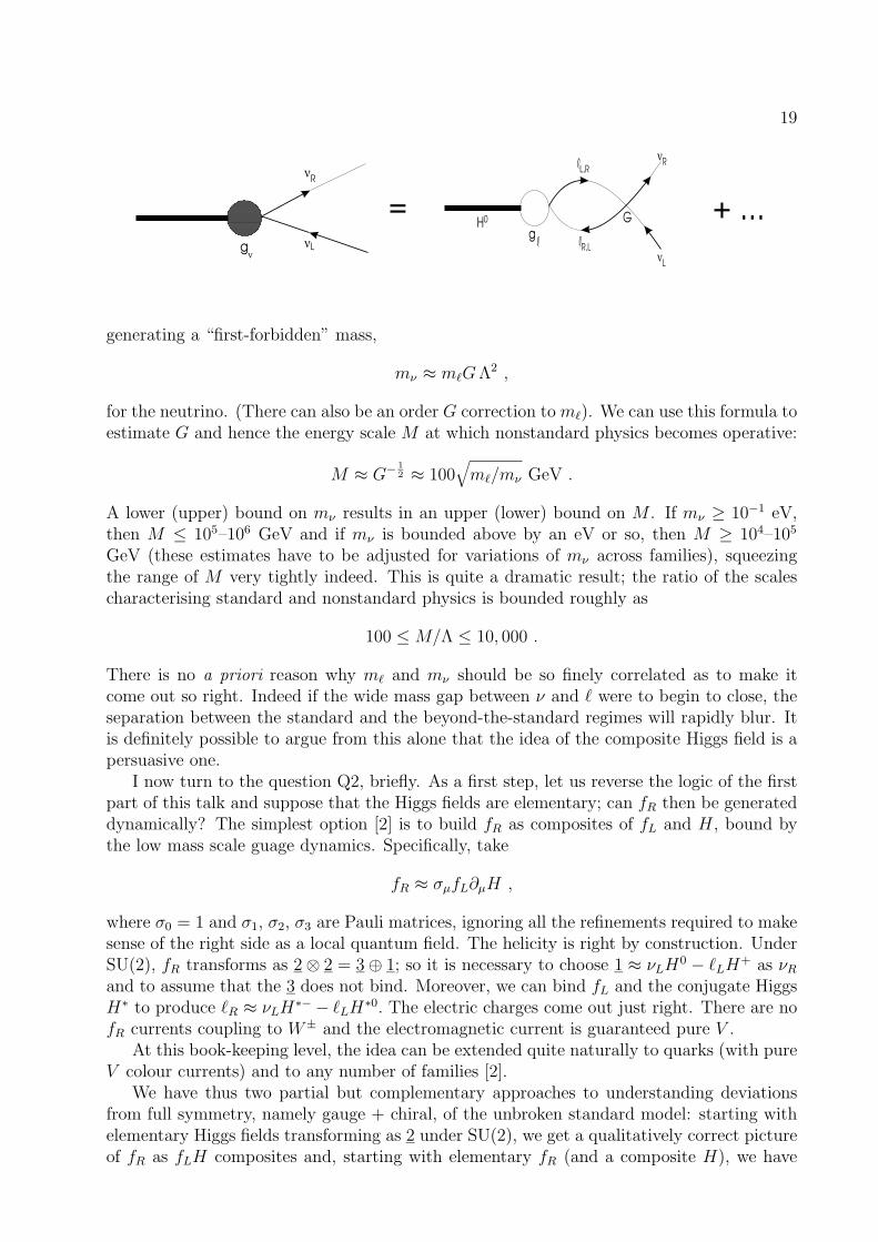
19

H0

lR,L

lL,R

gl

G

nR

nL

gn

nR

nL

= + ...

generating a “first-forbidden” mass,

mν ≈ m`G Λ2 ,

for the neutrino. (There can also be an order G correction to m`). We can use this formula toestimate G and hence the energy scale M at which nonstandard physics becomes operative:

M ≈ G− 12 ≈ 100

√

m`/mν GeV .

A lower (upper) bound on mν results in an upper (lower) bound on M . If mν ≥ 10−1 eV,then M ≤ 105–106 GeV and if mν is bounded above by an eV or so, then M ≥ 104–105

GeV (these estimates have to be adjusted for variations of mν across families), squeezingthe range of M very tightly indeed. This is quite a dramatic result; the ratio of the scalescharacterising standard and nonstandard physics is bounded roughly as

100 ≤ M/Λ ≤ 10, 000 .

There is no a priori reason why m` and mν should be so finely correlated as to make itcome out so right. Indeed if the wide mass gap between ν and ` were to begin to close, theseparation between the standard and the beyond-the-standard regimes will rapidly blur. Itis definitely possible to argue from this alone that the idea of the composite Higgs field is apersuasive one.

I now turn to the question Q2, briefly. As a first step, let us reverse the logic of the firstpart of this talk and suppose that the Higgs fields are elementary; can fR then be generateddynamically? The simplest option [2] is to build fR as composites of fL and H, bound bythe low mass scale guage dynamics. Specifically, take

fR ≈ σµfL∂µH ,

where σ0 = 1 and σ1, σ2, σ3 are Pauli matrices, ignoring all the refinements required to makesense of the right side as a local quantum field. The helicity is right by construction. UnderSU(2), fR transforms as 2 ⊗ 2 = 3 ⊕ 1; so it is necessary to choose 1 ≈ νLH0 − `LH+ as νR

and to assume that the 3 does not bind. Moreover, we can bind fL and the conjugate HiggsH∗ to produce `R ≈ νLH∗− − `LH∗0. The electric charges come out just right. There are nofR currents coupling to W± and the electromagnetic current is guaranteed pure V .

At this book-keeping level, the idea can be extended quite naturally to quarks (with pureV colour currents) and to any number of families [2].

We have thus two partial but complementary approaches to understanding deviationsfrom full symmetry, namely gauge + chiral, of the unbroken standard model: starting withelementary Higgs fields transforming as 2 under SU(2), we get a qualitatively correct pictureof fR as fLH composites and, starting with elementary fR (and a composite H), we have

20 CHAPTER 4. COMPOSITE FIELDS AND FERMION MASSES

a semi-quantitative picture of neutrinos, mν = 0. The really interesting question now iswhether they can be combined. Very naively, can we demand that the composite structuresH ∼ fLfR (or fRfL) and fR ∼ σµfL∂µH hold simultaneously? Clearly, the quantum numberbook-keeping will remain valid. For instance, the neutrino will remain massless even if fR

is dynamically generated as above since there is no νR current. To make dynamical sense,however, we have to do the dynamics. A possible approach is to start with a strongly chiralSU(2) × U(1) gauge theory and to generate both fR and H as manifestations of dynamicalsymmetry breaking a la Nambu-Jona-Lasinio. Appropriate non-perturbative amplitudesshould then signal both a mass gap in the fermion propagator and scalar “collective modes”breaking gauge invariance. This is of course a nontrivial task. But the reward for successwill be to rid the model, at least in principle, of all parameters except the gauge couplingsand the symmetry breaking scale.

The hospitality of the Institute of Mathematical Sciences, Chennai, where this work wasdone and of the School of Physics of the University of Hyderabad, where it was written up,is gratefully acknowledged.

Bibliography

[1] P. P. Divakaran and G. Rajasekaran, Mod. Phys. Letters 14, 913 (1999).

[2] P. P. Divakaran, Phys. Rev. D 60, 0550007 (1999).

21

22 BIBLIOGRAPHY

Chapter 5

Proof of absence of spooky actionat a distance in quantum correlations

C. S. Unnikrishnan∗

Tata Institute of Fundamental Research, Mumbai 400 005 &

Indian Institute of Astrophysics, Bangalore 560 034

Preface: Tribute to a teacher

I first met Rajaji during my undergraduate days, at a summer training program at theIndian Institute of Technology, Madras. I had come from a college in Kerala, and was beingoverwhelmed by the ambience - I was meeting live researchers for the first time. Then an‘examiner’ came to check whether we were doing fine with our projects. He did not looklike an academic. In fact he did look like an investigating officer. We were a bit worried.But the first interaction changed all that. The softness, the concern of a real teacher, andthe friendliness. I am really happy to be able to talk about some work that has caught hisattention, and has benefitted from his encouragement.

Quantum correlations

A physical flaw in local realism

The present interpretations of quantum measurement of entangled multiparticle systemsinvoke and support the notion of nonlocal state reduction by an unknown, spooky, action ata distance. There are two reasons for this. The standard quantum mechanical descriptionof multi-particle correlations uses the inseparable entangled wavefunction that describesthe total state of all the particles in a single entity. Then a measurement on one of theparticles instantaneously changes the entire wavefunction and changes the states of the othercorrelated particles. The second reason is the failure of the local hidden variable theories toreproduce the experimentally observed quantum correlations, and this failure is described bythe Bell’s theorem [1]. There has been a universal acceptance that this is due to nonlocality,rather than just due to the inadequacy of the notion of the physical reality used.

∗E-mail: unni.tifr.res.in

23

24 CHAPTER 5. PROOF OF ABSENCE OF SPOOKY ACTION

However, decades of debates and contemplation have not brought out the physical natureof the nonlocal influences that make the quantum correlations possible. Quantum nonlocalityeven violates the spirit of relativity, though not its signalling features. This suggests thatperhaps some deep and fundamental aspect is overlooked. In fact, a closer look at theEinstein-Podolsky-Rosen (EPR) argument [2] and the proof of the Bell’s theorem reveals afundamental physical flaw in the way the concept of physical reality is used. This is clearlyevident in the proof of the Bell’s theorem [1], as the inability of the formalism to accountfor any possible phases coherences at source encoding the prior correlations. In effect, thecorrelation function used in Bell’s theorem as well as in the standard local realistic theoriescompletely ignores the wave nature associated with microscopic particles.

The two distinct assumptions that go into the Bell’s theorem are that of locality andthe EPR physical reality [1]. Consider the measurement of the spin components on the twoparticles in two different directions a and b. The result of such a measurement is two-valuedin any direction. If A and B denote the outcomes +1 or −1, and a and b denote the settingsof the analyzer or the measurement apparatus for the first particle and the second particlerespectively, then the statement of locality is that

A(a,h1) = ±1, B(b,h2) = ±1 (5.1)

The outcome for the first particle is decided by the local setting a for the first analyzer, andby some hidden variable set h1. For the second particle the outcome is decided by the localsetting b and local hidden variables h2. The correlation of the outcomes is

P (a,b) =1

N

∑

(AiBi) (5.2)

The task of the theory is to calculate this function starting from suitable basic ingredientsof the theory. Bell chose to calculate this correlation by multiplying A(a,h1) and B(b,h2)and integrating over the distribution of the hidden variable h, since the assumption of realismdemanded that the outcomes were “there” even before the measurement was made. TheBell correlation is then

∫

dhρ(h)A(a,h1)B(b,h2), where∫

dhρ(h) = 1. The essence of Bell’stheorem is that the function P (a,b) has distinctly different dependences on the relative anglebetween the analyzers for a local hidden variable description and for quantum mechanics.

The crucial aspect to note is that the Bell correlation function has no way of incorporatingthe concept of phase or phase coherence since it uses the measured outcomes. The essenceof even single particle quantum behaviour is the inherent wave aspect and this is missed outin the local realistic formulation. Having identified such a serious physical flaw, the nextquestion to ask is whether it is possible to reproduce the correct correlation functions if theconcept of phase and phase coherence at source are incorporated in the formalism, keepingthe locality assumption intact. This has been shown to possible [3, 4]. There are localtheories with a definite reality for phases (a definite, though random, value for the phasebefore a measurement) that do not violate the Bell’s theorem.

Locality and separability of probability

Most of the local realists use separability of probabilities as a criterion for locality. Thisis fundamentally flawed. If P (a) and P (b) are the local probabilities, the joint probabilityP (a, b) = P (a) · P (b), if they are separable. The joint probability for measurements on anentangled system is not separable, and therefore local realists insist that there is nonlocality.

25

But separability of probability as a criterion for locality is not valid when there are wavelikeaspects, even when there is locality. The well known example is that of the Hanbury Brown-Twiss correlations [5]. The intensity of light from a source is measured by two detectors andcorrelated. The average of the intensity-intensity correlation (joint probability) is not theproduct of average intensities in each detector (local probabilities)! There is an interferencepattern as a function of the separation between the two detectors. There is no nonlocality.In fact, the effect is present classically. The Brown-Twiss correlations do not violate theBell’s inequality since classical wave aspects are involved, but this feature changes when onegoes to the complex ‘wave’ aspect of quantum systems. But already at the level of classicalwaves, it is evident that separability is not a good criterion for locality [4].

The correct correlation from locality and phase coherence

To illustrate the main aspects, let us consider the maximally entangled state

ΨS =1√2{|1,−1〉 − |−1, 1〉} (5.3)

where the state |1,−1〉 is short form for |1〉A |−1〉B , and represents an eigenvalue of +1for the first particle and −1 for the second particle if measured in any particular direction.ΨS is inherently nonlocal.

An experiment in which each particle is analyzed by orienting the analyzers at vari-ous angles θ1 and θ2 is considered next. The correlation P (a,b) = 1

N

∑

(AiBi) denotesthe average of the quantity (number of detections in coincidence − number of detectionsin anticoincidence), where ‘coincidence’ denotes both particles showing same outcome and‘anticoincidence’ denotes those with opposite outcomes.

We postulate that the correlation at source (conservation law) is encoded in the relativevalue, or the difference, of two internal variables φ1 and φ2 associated with the two particles.The value of φ can vary from particle to particle, being random, but the relative phasebetween the two particles in all correlated pairs is constant. Denoting θ1 − φ1 = θ andθ2 − φ2 = θ′ , we have θ − θ′ = θ1 − θ2 + φo.

We specify the local probability amplitudes as a complex number, whose square gives theprobability of transmission. These are CA = 1√

2exp(iθs) for measurements at analyzer A,

and for particle B is CB = 1√2exp(iθ′s) at analyzer B. In these expressions, the quantity

s is the spin (in units of h) of the particle. The locality assumption is strictly enforcedsince the two complex functions depend only on local variables and on an internal variabledetermined at source and then individually carried by the particles without any subsequentcommunication of any sort.

The probabilities for the outcomes of measurements at each end are now correctly repro-duced, for any angle of orientation. These probabilities are Re(C1C

∗1) = Re(C2C

∗2) = 1

2. The

amplitude correlation for an outcome of either (++) or (−−) of two maximally entangledparticles is

U(θ, θ′) = 2Re(C1C∗2)= Re{exp is(θ − θ′)}

= cos{s(θ − θ′)} = cos{s(θ1 − θ2) + sφo}. (5.4)

This, in contrast to the Bell correlation, carries the crucial wave aspects.

26 CHAPTER 5. PROOF OF ABSENCE OF SPOOKY ACTION

We rewrite this as U(θ1, θ2, φo) since all references to the individual values of the ‘hiddenvariable’ φ has dropped out. The square of U(θ1, θ2, φo) is the probability for coincidencedetection of the two particles through the analyzers kept at angles θ1 and θ2.

Since U2(θ1, θ2, φo) is the probability for a coincidence detection (++ or −−), the quantity(1−U2(θ1, θ2, φo)) is the probability for an anticoincidence (events of the type +− and −+).Then

P (a,b) = U2(θ1, θ2, φo) − (1 − U2(θ1, θ2, φo)) = 2U2(θ1, θ2, φo) − 1 (5.5)

For the case of the singlet state breaking up into two spin 1/2 particles, we set φo = π.Then the probability for joint detection through two Stern-Gerlach analyzers oriented atrelative angle θ1 − θ2 is

U2(θ1, θ2, φo) = sin2(1

2(θ1 − θ2)) (5.6)

P (a,b) = − cos(θ1 − θ2) = −a · b (5.7)

This is identical to the quantum mechanical predictions obtained from the singlet entan-gled wave-function and the Pauli spin operators.

Similar exercise can be carried out for other entangled states. We have reproduced thecorrect quantum correlations in a local theory [3]. The most striking implication is thatthere is no spooky state reduction at a distance.

Proof of absence of spooky action at a distance

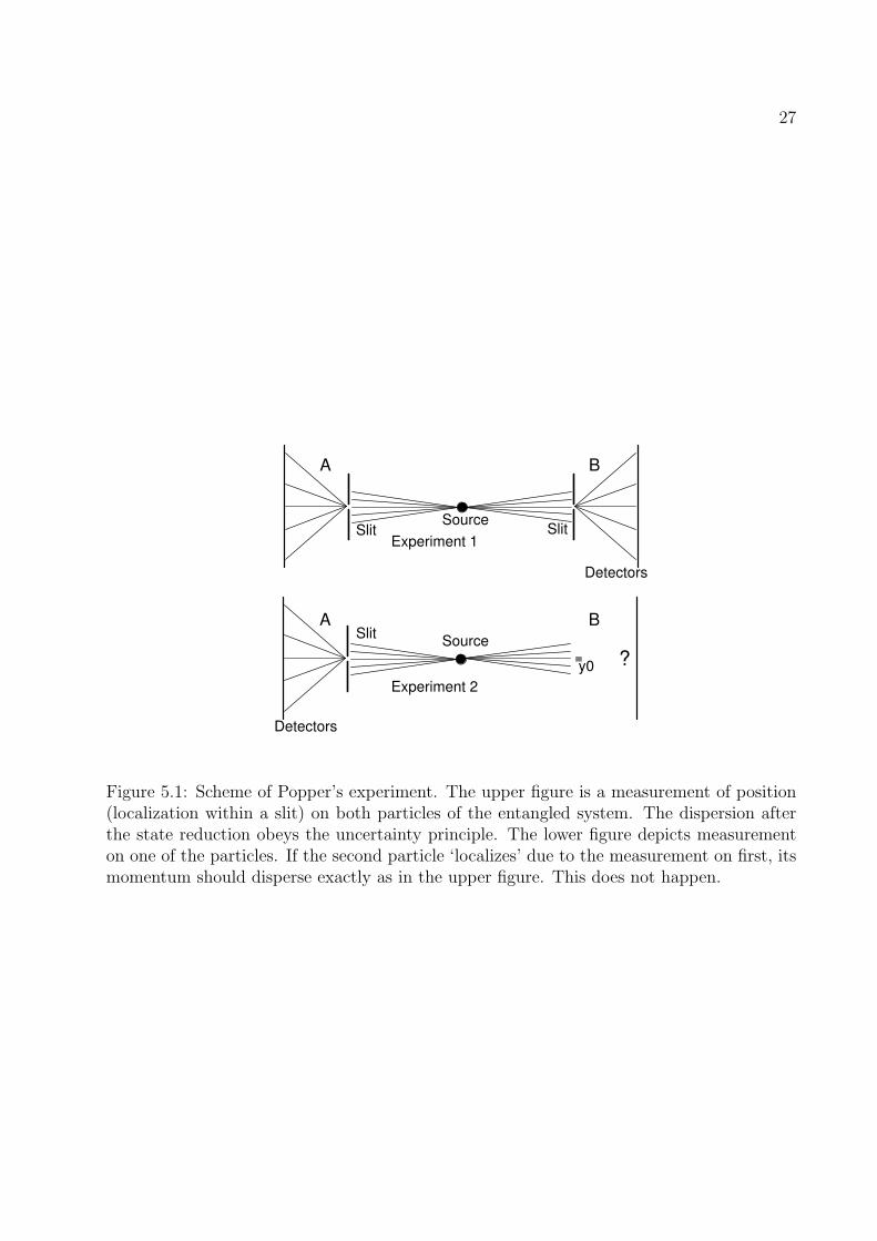
Now we point out the proof from experiments that there is no state reduction at a distancedue to partial measurements on entangled multiparticle systems. A state reduction in quan-tum systems is characterized by two essential aspects. a) The state assumes a definite valuefor an observable or a set of observables. b) The dispersion in any noncommuting observablechange so as to satisfy the uncertainty principle. In classical systems the second aspect isirrelevant. Clearly, if a measurement on one particle reduces the state of the companion par-ticle then the dispersion associated with the noncommuting observable should also changeas a result of the measurement [3, 4]. For example, if the position of the first particle ismeasured to be x1 with spread ∆x1, the second particle’s position can be predicted withgood certainty using the conservation law. If this amounts to a true state reduction to adefinite position x2 with uncertainty ∆x2, then its momentum should spread out to satisfy∆p2 ≥ h/∆x2. This does not happen, since if it did, signal locality could be violated – wecould send signals faster than light. This becomes possible since ∆x1 ∼ ∆x2 can be made assmall as one wishes and then ∆p2 will become larger than any initial spread of the originalstate. This feature is not observable in experiments with spin, since it is a bounded variable.Remarkably, K. Popper had proposed [6] such an experiment, two years before the EPRargument. Recently this experiment was performed [7] and, consistent with our assertionbased on signal locality, no additional spread of momentum of the second particle was seen.This clearly proves that there is no state reduction at distance. It also shows that termslike quantum teleportation are inappropriate. What is seen in those experiments are priorcorrelations encoded in the initial phase coherence.

27

?Source

Slit

SourceSlit Slit

A

A

B

B

Experiment 1

Experiment 2

Detectors

Detectors

y0

Figure 5.1: Scheme of Popper’s experiment. The upper figure is a measurement of position(localization within a slit) on both particles of the entangled system. The dispersion afterthe state reduction obeys the uncertainty principle. The lower figure depicts measurementon one of the particles. If the second particle ‘localizes’ due to the measurement on first, itsmomentum should disperse exactly as in the upper figure. This does not happen.

28 CHAPTER 5. PROOF OF ABSENCE OF SPOOKY ACTION

Bibliography

[1] J. S. Bell, Speakable and unspeakable in quantum mechanics (Cambridge University Press,1987).

[2] A. Einstein, B. Podolsky, and N. Rosen, Phys. Rev. 47, 777 (1935).

[3] C. S. Unnikrishnan, Current Science 79, 195 (2000).

[4] C. S. Unnikrishnan, Annales de la Fondation Louis de Broglie (Paris) 25, 363 (2000).

[5] R. Hanbury Brown and R. O. Twiss, Nature 178, 1447 (1956).

[6] See K. R. Popper, in Open Questions in Quantum Physics, Eds. G. Tarozzi and A. vander Merwe, (D. Reidel Publishing Co., 1985).

[7] Y-H. Kim and Y. Shih, Found. Phys. 29, 1849 (1999).

29

30 BIBLIOGRAPHY

Chapter 6

Are Accelerators Needed forHigh-Energy Physics?

Srinivas Krishnagopal∗,

Centre for Advanced Technology,

Indore 452013

Introduction

When the organizers of the Rajaji Seminar invited to me speak here, I accepted at once withpleasure, but also with some bemusement. I couldn’t figure out why I was being invited. Iam not a student of Prof. Rajasekaran’s, I am not a ‘grand-student’ of Prof. Rajasekaran’s,I am not a particle theorist, I am not a high-energy physicist, and I am not even that low-energy approximation, a nuclear physicist. The only explanation I could think of was thatthere had been some kind of mistake. Perhaps the organizers wanted to invite a Srinivasan,or a Krishnan or a Gopalan, and their computer found my name in its database! A coupleof months passed without any communication from the organizers, and that seemed to lendcredibility to my theory. But one day I received an email asking for the title of my talk. So,after sending in the most provocative title I could think of, I recalled my interaction withProf. Rajasekaran.

Over the last five years, I have been running at CAT a DST-funded winter school on thePhysics of Beams. The purpose of this School is to attract bright students to this new, andin India unknown, field. In this context I was told that Prof. Rajasekaran was someone whohad been championing the need to build new accelerators at higher energies. His point isthat if new experiments, at higher energies, are not forthcoming, then high-energy physicsis in the danger of becoming sterile. I had of course heard of Prof. Rajasekaran, thoughI had never met him, so I sent him a letter asking if he would speak at the School onthis perspective, and he graciously agreed. At the School he gave an extremely lucid andenjoyable overview of particle physics for the students. At the end of his talk he stronglyemphasised the importance of looking for new techniques of acceleration, that will allow usto do experiments at much higher energies than are possible today: beyond, say, 10 TeV.This endorsement of accelerator physics by a leading particle theorist had a deep impact onthe students, and many of them expressed interest in the field, with a couple of them coming

∗E-mail:skrishna@cat.ernet.in

31

32 CHAPTER 6. ARE ACCELERATORS NEEDED FOR

to CAT in the summer to do projects in beam physics. Prof. Rajasekaran was also kindenough to come again a few years later, and give a similar talk at the Fourth School.

The theme of my talk today will be along the lines delineated above: ideas for newacceleration techniques, and a discussion on the need of accelerators for high-energy physics.

Present methods of acceleration

DC accelerators

The simplest way to accelerate a charged particle is to ‘drop’ it in an electrostatic potential.This is the principle of DC accelerators, such as van de Graff accelerators. The limitationof this kind of accelerator is that it is a ‘single-push’ device; since electrostatics is conser-vative, once the accelerated particle comes out of the accelerator, you cannot take it backto the ‘top of the hill’ for reacceleration (without losing all the energy gained). Therefore,DC accelerators are limited by practical issues such as the maximum voltage that can besustained before breakdown. Typically this is around 20 MV, which means that you cannotaccelerate electrons or protons to more than around 20 MeV by this technique.

RF accelerators

In order to accelerate charged particles to beyond around 20 MeV, one needs to providemultiple ‘pushes’, and for this one needs a non-conservative or time-varying field, i.e. anelectromagnetic field. The vast majority of accelerators today therefore use the principleof RF acceleration. Here, electromagnetic radiation, typically in the radio-frequency (RF)range, fills a cylindrical cavity, which supports a TM mode (that has an axial electric field).Since a cylindrical cavity only supports modes with a phase velocity greater than c, it isnecessary to slow down the electromagnetic wave by periodically loading the structure. Acharged particle beam injected along the axis of this loaded cylinder will now be acceler-ated. Because of the time-varying nature of the fields, it is possible to accelerate particlesrepeatedly, either in the same RF cavity (circular accelerator), or in successive ones (linearaccelerator).

The size of an accelerator depends on the accelerating gradient produced in the RF cavity.For normal conducting cavities, that are made of copper and operate at room temperature,typical accelerating gradients that one can achieve are of the order of 10 MV/m. With thisgradient, for example, a 1 TeV linear collider would need to be 100 km long!

Therefore, for very high-energy accelerators, people today use superconducting RF cav-ities. These are typically made of Niobium, and operate at 4.2 K or 1.8 K. Because thecavities are superconducting, there is very little power dissipation in the cavities, and there-fore they are very efficient. One can also achieve higher gradients in these cavities; typicallyof the order of 100 MV/m (or actually many tens). For example, the TESLA collider beingbuilt in Germany is designed for a beam energy of 1 TeV, and will be 30 km long.

The above numbers make one thing very clear. RF acceleration can produce gradientsof no more than 100 MV/m, and with this gradient one cannot cross the 10 TeV frontier;even a multi-TeV collider will be many tens of kilometres long. In order to cross the 10TeV frontier, therefore, one needs to look at new methods of acceleration, that can providehigher, much higher, gradients.

33

Plasma-based Accelerators

The basic idea of plasma acceleration was first proposed and studied by Tajima and Dawsonin 1979 (T. Tajima and J.M. Dawson, Phys. Rev. Lett. 43, 267 (1979)). Since the mid-90s,there has been an explosion in the field, with a number of very exciting experimental results.

There are different schemes of plasma acceleration, the most promising of which is LaserWakefield Acceleration (LWFA). In this scheme, a short pulse (< 1 ps), high intensity (> 1018

W/cm2) laser is shot through a gaseous medium. The ponderomotive force of the laser excitesa longitudinal plasma wave, with a velocity close to the speed of light. If, at the same time,one injects an electron beam into the plasma, the electron beam can be accelerated.

In a number of experiments performed around the world, many milestones have beenachieved. Accelerating gradients of 100 GV/m, actual acceleration to an energy of 400 MeV,and acceleration of a charge of around 1 nC, have all been demonstrated. Of course, manyproblems remain. The main problem is that plasma acceleration has been demonstratedonly over distances of a few mm, largely because of the diffraction of the laser over largerdistances. Second, the electrons typically have a large energy-spread (almost 100%), so thatthe actual number of electrons at the highest energy may be small. Much work is therefore onto understand and overcome these problems. So, while the principle of plasma accelerationis well established, we are still far from building a plasma accelerator.

However, the potential is enormous. An accelerating gradient of 100 GV/m has alreadybeen demonstrated, which is three orders of magnitude higher than the best you can achievethrough RF acceleration. Which means in a plasma accelerator one can achieve 1 GeVacceleration in 1 cm, and 10 TeV in 100 m! The 1 TeV TESLA collider could be built in 10m (rather than 30 km). Of course, it may not be possible to sustain acceleration in a plasmaaccelerator for more than a few cms, but in this case one could think of having multipleacceleration modules (exactly as one has many RF cavities in a linear RF accelerator).

Plasma acceleration is a totally new and exciting way of accelerating particles. Whilethere is a long way to go before one can actually demonstrate a plasma accelerator, thereis also much reason to put in that effort. If successful, plasma acceleration would make itpossible to cross the 10 TeV frontier.

Are accelerators needed for high-energy physics?

In general, the answer to this question is obviously ‘yes’. Even theorists must pay at leastlip service to the importance of getting theories confirmed by experiments. The question istherefore being asked in the more restricted context of high-energy physics in the country.

In India, all experimental high-energy physics is done in the form of international col-laborations: at CERN, Fermilab, etc. This is obviously a good thing, because it gives usaccess to data from the latest experiments, enables international exposure, competitive re-search, etc. And the quality of this work has been very high. However, it seems to me thatone can achieve greater depth and a broader base in the field only if there is experimen-tal activity within the country. Obviously, one is not talking about exploring the energyfrontier, but rather about experiments at lower energies, such as B-factories at 5 GeV andtau/charm factories at 2.5 GeV. In particular, the Chinese experience shows that interestingand competitive research can be done even at lower, multi-GeV, energies.

The obvious problem with doing high-energy experiments within the country is the lackof an accelerator: a sufficiently serious problem that completely justifies the present state

34 CHAPTER 6. ARE ACCELERATORS NEEDED FOR

of affairs. However, since the last few months, there is now working at CAT a 450 MeVelectron storage ring, INDUS-1, which is by far the highest energy accelerator in the country.Therefore the ability to build a low-energy storage ring has been demonstrated. Further,work has started on building INDUS-2, a 2.5 GeV storage ring, which, in my opinion, shouldbe working in around five years from today. Once that happens, we will have shown theability, in essence, to build a multi-GeV collider.

In the changed scenario, where multi-GeV accelerators can be built in thecountry in a time frame that is not unduly long, it seems that the possibil-ity of doing high-energy physics experiments within the country warrants re-examination.

The point I am making is a limited one: that an avenue long ignored, should now beexplored. It may be that, after serious thought, the conclusion is that the time is still notripe for an indigenous experimental high-energy physics programme; perhaps because by thetime say a tau/charm factory is built, all the interesting experiments will have been done.But that conclusion should be the result of mature deliberation, and not a consequence ofeither inertia or a casual brush-off.

In this spirit let me offer the following points for thought:(a) After INDUS-2 is built, say five years from now, INDUS-1 (450 MeV) will be largelyredundant. Can we then convert INDUS-1 into a collider?(b) Can one do parasitic fixed-target experiments at INDUS-2 (2.5 GeV)?(c) Can one build a new multi-GeV electron storage-ring collider, perhaps as part of an Asiancollaboration?(d) Can one think of a CEBAF-type continuous electron beam facility for nuclear physics aswell as high-power free-electron lasers?(e) Can one think of a multi-GeV linear collider, again perhaps as part of an Asian or othercollaboration?

To summarize: with the commissioning of INDUS-1, one can assert that it is now becom-ing possible to build a multi-GeV circular accelerator in India; therefore, this is the right timeto start thinking about a possible experimental programme in high-energy physics withinthe country.

Finally, I would like to congratulate Prof. Rajasekaran on a long and fruitful researchcareer, and wish him all the best for an equally active research career in the years to come.

Chapter 7

Ortho and Para SupersymmetricQuantum Mechanics of Arbitrary

Order

Avinash Khare∗,

Institute of Physics, Sachivalaya Marg,

Bhubaneswar 751005, Orissa, India

It is a great honour to talk at the Rajaji Symposium. Rajaji is one of the stalwarts inhigh energy physics in this country. He is an excellent speaker and has inspired a generationof High Energy Physicists. Apart from being a good phenomenologist, he has also done someinteresting work in mathematical physics. My collaboration with him is in fact in this field.

I first saw Rajaji in 1971 when he give his famous nonabelian gauge theory lectures atSINP, Calcutta where I was a graduate student. I must confess that I did not appreciate itssignificance at that time. Our first strong overlap was when we were together for a month atUniversity of McMaster, Canada in 1990. We stayed together and that is when I discoveredthe weakness of Rajaji for Pizza and Coke !

In early 1992 both Rajaji and myself attended a workshop at ISI, Calcutta. While Italked about Chern-Simons term and charged vortices, he talked about ortho-fermions andortho-bosons the work which he had done with Dr.A.K. Mishra from his institute. As usualhis seminar was very clear and I immediately realized that something can be done.

Let me explain why I felt so. Since 1984 I have been working in the area of supersymmetricquantum mechanics (SQM) where there is a symmetry between bosons and fermions andsince 1990 I have been working about anyons and fractional statistics. Further, only fewmonths ago, I had written a paper about para-supersymmetric quantum mechanics (PSQM)[1], where there is a symmetry between bosons and para-fermions. So I felt that one couldnow construct ortho supersymmetric quantum mechanics (OSQM) where there will be asymmetry between bosons and ortho-fermions. I suggested this to Rajaji and we exchangedour papers and agreed to meet the next day after reading each others papers. We haddetailed discussions on the next day and we agreed to pursue this problem. The entire workincluding paper writing was done via e-mails. We had disagreement and fights but it is tothe credit of Rajaji that he never took these physics fights personally. I am glad to note

∗khare@iopb.res.in

35

36 CHAPTER 7. ORTHO AND PARA SUPERSYMMETRIC

here that when in 1995 Cooper, Sukhatme and I wrote a Physics Reports on SQM [2], weincluded this important work there.

To appreciate this work, let us first explain what one means by ortho-Fermi statistics[3]. This statistics is characterized by a new exclusion principle which is more “exclusive”then the Pauli exclusion principle: an orbital state shall not contain more than one particle,whatever the spin direction. Further, the wave function is antisymmetric in spatial indicesalone, with the order of the spin indices frozen.

For the special case of a single ortho-fermion of order p (which is what is required forconstructing OSQM), the creation and annihilation operators c+

α and cα satisfy (α, β =1, 2, . . . , p).

cαc+β + δα,β

p∑

r=1

c+r cr = δα,β ; cαcβ = 0 . (7.1)

This equation implies thatc1c

+1 = c2c

+2 = cpc

+p . (7.2)

For comparison sake, let us notice that the fermionic operators b, b+ satisfy

{b, b+} = 1 , b2 = 0 = b+2 , (7.3)

while the para-fermions of order p satisfy

[[a+, a], a] = −2a , [[a+, a], a+] = 2a+ , ap = (a+)p = 0 . (7.4)

Let us now recall how, using the above algebras (10.3) and (10.4), SQM and PSQM havebeen constructed. In SQM one defines super charge Q,Q+ satisfying

{Q,Q+} = 2H , Q2 = 0 = (Q+)2 , [H,Q] = 0 = [H,Q+] , (7.5)

while using eq. (10.4), Rubakov and Spiridomov [4] wrote down the following PSQM of order2

Q3 = 0 = (Q+)3 , [H,Q] = 0 = [H,Q+] , (7.6)

Q2Q+ + QQ+Q + Q+Q2 = 4QH . (7.7)

These and other authors were unable to generalize relation (10.7) to any arbitrary order p. Infact, Durand et al. [5] discussed this issue in some detail and concluded that the multi-linearpart of the higher order PSQM (p ≥ 3) cannot be characterized with one universal algebraicrelation. However, subsequently I showed [1] that this is not so and that the PSQM of orderp is characterized by the nontrivial relation

QpQ+ + Qp−1Q+Q + . . . + Q+Qp = 2pQp−1H , p = 1, 2, . . . , (7.8)

in addition to the obvious generalization of eq. (10.6). Note that unlike in SQM ( and alsoin OSQM, as we shall see shortly), in PSQM, the Hamiltonian cannot be written in termsof supercharges alone, since the inverse of Qp−1 does not exist. Rajaji was unhappy aboutthis feature and subsequently we [6] gave an alternative formulation (see below) where oneis able to express H in terms of PSQM charges.

Since the ortho-Fermi operators satisfy relations (10.1) and (10.2), we suggested thatOSQM should be characterized by the algebra [7]

QαQβ = 0 , [H,Qα] = 0 = [H,Q+α ] , (7.9)

37

QαQ+β + δα,β

p∑

r=1

Q+r Qr = 2δαβH . (7.10)

From here we deduce that Q1Q+1 = Q2Q

+2 = . . . = QpQ

+p .

A useful representation of SQM algebra (10.5) is given by

Q =(

0 p − iW0 0

)

, 2H =[

p2 + W 2 − W ′ 00 p2 + W 2 + W ′

]

, (7.11)

where W ′ means derivative with respect to x. Similarly a useful representation of the PSQMof order p is given by

(Q)αβ = (P − iWβ)δα,β+1 , (Q+)αβ = (P + iWβ)δα+1,β (7.12)

while the corresponding H is a (p + 1) × (p + 1) diagonal matrix: 2H = hrδrr where

hr = P 2 + W 2r − W ′

r + Cr , r = 1, 2, . . . , p (7.13)

hp+1 = P 2 + W 2p + W ′

p + Cp . (7.14)

This H commutes with the supercharges provided

W 2r + W ′

r + Cr = W 2r+1 − W ′

r+1 + Cr+1 , r = 1, 2, . . . , p − 1 , (7.15)

with the arbitrary constants C1, C2, . . . , Cp satisfying the constraint

p∑

r=1

Cr = 0 . (7.16)

On the other hand, the p OSQM charges Qα are again (p + 1)× (p + 1) matrices as given by

(Qα)rs = (P − iWα)δr,1δs,α+1 (7.17)

while the corresponding H is a (p + 1) × (p + 1)diagonal matrix: 2H = Hrδrr where

H1 = P 2 + W 21 + W ′

1 , Hr+1 = P 2 + W 2r − W ′

r , r = 1, 2, . . . , p . (7.18)

On further demanding the condition Q1Q+1 = . . . = QpQ

+p , we get the constraint

W 2r + W ′

r = W 2s + W ′

s , r, s = 1, 2, . . . , p . (7.19)

Some of the important salient features of SQM, PSQM and OSQM are

1. Whereas in SQM, all the excited states are always two-fold degenerate, in OSQM oforder p, all the excited states are (p+1)-fold degenerate. On the other hand, in PSQMof order p, p’th and higher excited states are (p+1)-fold degenerate while nothingdefinite can be said about the other excited states.

2. In SQM and OSQM, all the energy eigenvalues are positive semidefinite with the groundstate energy E0 = 0 (> 0) corresponding to unbroken (broken) symmetry, no suchconclusion can be drawn in PSQM case unless C1 = C2 = . . . = Cp = 0 in which casesymmetry is unbroken (broken) if E0 = 0 (>).

3. A model of conformal SQM, PSQM and OSQM has also been constructed.

38 CHAPTER 7. ORTHO AND PARA SUPERSYMMETRIC

One of the draw back of the PSQM as formulated here is that, H is not expressible in termsof Q and Q+. We have given [6] a new formulation of PSQM where this defect can be cured.In particular, we showed that, in the new formulation, the constants C1, C2, . . . , Cp = 0 andthen H2 is given in terms of Q and Q+ by [6]

H2 =1

4

[

(Q+Q)2 + (QQ+)2 − QQ+Q+Q]

. (7.20)

We also use it to construct the PSQM of infinite order whose algebra (i.e. H = 12QQ+)

corresponds to the single mode version of the algebra describing Greenberg’s infinite statistics[8].

Bibliography

[1] A. Khare, J. Phys. A 25 (1992) L749; J. Math Phys. 34, 1277 (1993).

[2] F. Cooper, A. Khare and U.P. Sukhatme, Phys. Rep. 251, 267 (1995).

[3] A.K. Mishra and G. Rajasekaran, Pramana 36, 537 (1991); ibid 37, 455 (1991) (E); ibid38, L4111 (1992).

[4] V.A. Rubakov and V.P. Spiridonov, Mod. Phys. Lett. A 3, 1337 (1988).

[5] S. Durand, M. Mayrand, V. Spiridonov and L. Vinet, Mod. Phys. Lett. A 6, 3163 (1991).

[6] A. Khare, A.K. Mishra and G. Rajasekaran, Mod. Phys. Lett. A 8, 107 (1993).

[7] A. Khare, A.K. Mishra and G. Rajasekaran, Int. J. Mod. Phys., A 8, 1245 (1993).

[8] O.W. Greenberg, Phys. Rev. Lett. 64, 705 (1990).

39

40 BIBLIOGRAPHY

Chapter 8

Fock Spaces and Quantum Statistics

A.K. Mishra∗,

The Institute of Mathematical Sciences,

Taramani, Chennai 600113, India

Abstract.A brief description of new forms of quantum statistics is provided. It is demonstrated

that a concept of generalized Fock spaces enables one to obtain a unified picture for variousstatistics and associated algebras.

Many new kinds of quantum statistics were discovered during the last decade. Thesediscoveries owe their origin to various fundamental questions concerning the physical statesof matter. Thus a possible small violation of Pauli’s exclusion principle has led to theformulation of quons which obey infinite statistics. A notion of impenetrability of pointparticles in one dimension has given rise to null statistics. A whole new family of quantumstatistics viz. orthostatistics were obtained while analyzing the consequences of infiniterepulsion between electrons occupying the same orbital state.

In dimensions equal or greater than three, particle statistics are classified according to therepresentations of permutation group, and in two dimension, via braid group representations.It has been often argued that particles in a one-dimensional system would not cross eachother, and so the notion of statistics is void in 1-D [1]. It is important to note here thatwhatever approach one uses for constructing the statistics, the exercise ultimately leads tospecifying the permissible physical states for the system.

In this article, we describe various new forms of recently discovered quantum statistics.and highlight the underlying motivation for this endeavour. A number of these statisticshave been constructed at our Institute in collaboration with Professor G. Rajasekaran.

In spite of the fact that a large literature which now exists, a unified picture for variousstatistics and their associated algebra has not emerged. To achieve this objective, we haveintroduced the concept of generalized Fock spaces. Starting with this basic notion, it ispossible to show that more than one statistics can be postulated in a given Fock space,and many different algebraic realizations can be constructed for any particular statistics. Inthe theory of generalized Fock spaces, the key element is the notion of independence of thepermutation ordered states. The largest linear vector space constructed in this way is the

∗E-mail: mishra@imsc.ernet.in

41

42 CHAPTER 8. FOCK SPACES AND QUANTUM STATISTICS

super Fock space. The subsequent specification of a subset of states in this space as null statesleads to many reduced Fock spaces. All these spaces are collectively called as generalizedFock spaces. We construct creation (c†), annihilation (c) and number (N) operators in thegeneralized Fock spaces. The creation and annihilation operators, even for a particular Fockspace, are not unique. Consequently, many statistics and algebras can exist in a given Fockspace. On the other hand, a universal representation for the number operator valid for allforms of statistics and algebra exists. A brief description of this formalism is also providedin this article.

The Bose and Fermi statistics are based on the symmetry postulates, and these aredescribed through canonical commutation and anticommutation relations, respectively.

[cj, c†k]−+ = δjk ; [cj, ck]−

+= 0 (1)

Many new kinds of quantum statistics are obtained by appropriate generalizations of theseknown commutation relations. The eq.(1) can be equivalently written as

[ci, [ci, c†k]−+ ] = 2δijck ; [ci, [c

†j, c

†k]−+ ] = 2δijc

†k

−+ 2δikc

†j (2)

[ci, [cj, ck]−+] = 0 (3)

The general solutions for c and c† satisfying eqs.(2,3) lead to parabose and parafermi statis-tics, of which fermi and bose statistics are specific examples [2, 3].

Next, the replacement

[cj, c†k]−+ = δjk → [cj, c

†k]q = δjk ≡ cjc

†k + qc†kcj = δjk ; −1 < q < 1 (4)

has led to the concept of quons which obey infinite statistics [4, 5, 6, 7]. In this statistics,each permuted state is an independent state. For q = + (−)1, fermionic anticommutation(bosonic commutation) relation is recovered. But for q = 1 − |ε| (ε is an infinitesimal), asmall violation of Pauli’s exclusion principle results.

As a counterpoint to infinite statistics, null statistics can also be constructed [8]. Inthis statistics, no permutation is allowed and particles are frozen in their initial order. Thequanta satisfying null statistics are characterized through the algebra

ckc†j = 0 for k 6= j ; cjc

†j = 1 −

∑

k<j

c†kck ; cicj = 0 for i < j (5)

The number operator for infinite statistics when q = 0 (cic†j = δij) is

Nk =∑

ng ..nk..nm

∑

µ

(

c†ng

g . . . c†nk

k . . . c†nm

m ; µ)

c†kck

(

cnm

m . . . cnk

k . . . cng

g ; µ)

(6)

where µ labels each distinct permutation of operators inside the bracket. Interestingly, if thesummation over µ is removed, the number operator for the null statistics is obtained.

Nk =∑

n1,n2...nk

c†n11 c†n2

2 . . . c†nk

k c†kckcnk

k . . . cn22 cn1

1 (7)

The infinite statistics is obtained by modifying the canonical commutation relation betweenc and c† to a q-commutator. Note that no cc relation exists in infinite statistics, as each

43

permuted state is an independent state. Instead of modifying the cc† relation as in eq,(4), ifcc relation in eq.(1) is q deformed

[cj, ck]−+

= 0 → [cj, ck]q = 0 ≡ cjck + qckcj = 0 (8)

(where q is real and finite), a q-statistics which is based on quantum group algebra is obtained.The constraint that an orbital state shall not contain more than one particle irrespective

of their spin direction has led to the formulation of a new family of quantum statistics,namely, orthostatistics [9, 10, 11]. These statistics are described using the algebra

ckαc†pβ ± δαβ

∑

γ

c†pγckγ = δkpδαβ (9)

ckαcpβ ± cpαckβ = 0 (10)

Here k, p refer to spatial coordinates and α, β denote spin components. The positive andnegative signs respectively correspond to orthofermi and orthobose statistics. A multiparticlewave function for othofermions (orthobosons) is antisymmetric (symmetric) in k,m, whereasno symmetry constraint is required for the indices α, β. An exchange in the former set ofindices lead to fermi (bose) statistics, whereas the later satisfy infinite statistics. Thusortostatistics represent first instance wherein quanta having composite statistical character(that is indices belonging to different class exhibit uncorrelated permutation properties) isproposed.

Orthostatistics arise when particles occupying same orbital mutually interact throughinfinite repulsive potential. We have earlier shown that a system of electrons subject to nodouble occupancy in a single orbital state can be described by two distinct set of algebras,one corresponding to orthofermi statistics and other defining the Hubbard statistics [9, 10].But recently it has been shown that such a system is described by the orthofermistatistics[12].

It has been shown earlier that infinite statistics arises as a consequence of deformationof canonical commutation or anticommutation relation. Similarly, a deformation of theorthostatistics algebra, that is,

ckαc†mβ + qδαβ

∑

γ

c†mγckγ = δkmδαβ , −1 < q < 1 (11)

gives rise to doubly-infinite statistics; one with respect to the pair of indices (k,m) and otherfor the pair (α, β) [10].

The canonical commutation relation follows by mapping {x, ∂∂x} to {b, b†}. This shows a

close connection between particle statistics and differential calculus. Surprisingly, no map-ping of the differential dx to a creation operator had been reported. We have completedthis task both for commutative and noncommutative spaces. In this case of noncommuta-tive space, the mapping of dx to a creation operator has led to a new notion of statisticaltransmutation under particle exchange [13].

To understand the various types of statistics and algebras of creation and annihilationoperators, and interconnections among them, we start with the underlying space of allowedstate vectors or Fock space. Given a set of quantum numbers g, h, i... with the respectiveoccupancy being ng, nh, ni..., all possible multiparticle state vectors are

|ng, nh . . . nm; µ〉 , µ = 1, 2 . . . s (12)

44 CHAPTER 8. FOCK SPACES AND QUANTUM STATISTICS

where s is the total number of distinct permutations and µ labels each of these permutedstates. We assume the existence of a unique vacuum state

|0〉 ≡ |0, 0, 0 . . . 0〉 (13)

All these states are linearly independent, but need not be orthogonal or normalized

〈n′

g, n′

h . . . n′

m; α|ng, nh . . . nm; ν〉 = δn′

gngδn

′

hnh

. . . δn′

mnmMµν (14)

with M being a s × s hermitian matrix. We choose it to be positive definite.From the set of linearly independent state vectors, an orthonormal set of vectors {‖

ng . . . nm; µ À} can be obtained

‖ ng . . . nm; µ À=∑

ν

Xνµ|ng . . . nm; ν〉 (15)

Alternatively, starting with the orthonormal vectors {‖ ng . . . nm; µ À}, the vectors{|ng, nh . . . nm; µ〉} can be constructed by taking the inverse of relation (15). X is a nonsin-gular matrix. Although X is not unique and depends on the particular orthogonalizationprocedure, we have

M−1 = XX† (16)

Choosing a nonsingular matrix X and determining the inner product matrix M as abovewill ensure the positivity of the matrix M .

The set of state vectors considered here constitute super Fock space. Infinite statisticsresides in this Fock space. Using the projection operator

P (ng . . . nk . . . nm) =∑

λ,ν

|ng . . . nm; ν〉(M−1)νλ 〈ng . . . nm; λ| (17)

the number operator can be written as

Nk =∑

ng ...nk...nm

nkP (ng . . . nk . . . nm) (18)

which satisfies the following properties

Nk|ng . . . nk . . . nm; µ〉 = nk|ng . . . nk . . . nm; µ〉 ; [Nk, Nj]− = 0 (19)

The creation operator is defined as

c†j =∑

ng ...nj ...nm

∑

µν

Aµν |1jng . . . nj . . . nm; µ〉 〈ng . . . nj . . . nm; ν| (20)

and cj as the hermitian conjugate of c†j. Aµν are a set of arbitrary (complex) numbers. Evenat this stage, it is possible to verify that

[c†j, Nk]− = −c†j δjk (21)

The ordered state vectors can be constructed using a string of c† acting on the vacuumstate. Consequently we also have

∑

ν

Aµν Mνλ = δµλ ; A = M−1 (22)

45

We have provided here a unique representation of the number operator. But manydifferent representations of creation and annihilation operators are possible through differentchoices of matrices A, X and M . The number operator N can be expressed in terms of c†

and c by solving Eqs.(17,18) and (20). Since c† and c are not uniquely defined many differentexpressions for N in terms of c†, c can be obtained.

Next we consider reduced Fock spaces. All known forms of statistics other than theinfinite statistics reside in reduced Fock spaces, which are obtained by postulating relationslike

∑

µ

Bpµ|ng, nh . . . ; µ >= 0 ; p = 1, 2, . . . r (23)

where r < s and Bpµ are constants. The vector space dimension in the sector {ng, nh . . .} is

now reduced to d = s − r. The formalism developed for the super Fock space is also validfor reduced Fock spaces. But µ and ν now ranges from 1...d, and X, M and A are d × dmatrices.

Arbitrariness in the matrix A appearing in the creation operator expression (20) canbe exploited to generate many relations involving c† c†. Therefore, many different formsof statistics specified by different c† c† relations can be constructed in a given Fock space.All these statistics are interconnected. No connection exists between the statistics and theassociated algebras residing in different Fock spaces. It may also be mentioned here thatmultiplicity of statistics are not possible in the super Fock space and in the Fock space offrozen order. Only infinite and null statistics respectively reside in these two Fock spaces.But even here, many algebras involving c and c† are possible.

Thus, by decoupling the notion of the underlying Fock space from c and c†, we are able todefine different forms of statistics in a representation independent manner. Subsequently, onecan construct creation, annihilation operators and their algebra in any desired representation.

The general formalism not only unifies and classifies various forms of quantum statis-tics, but also enables us to construct many new kinds of statistics and algebras for singleand two-indexed systems in a systematic manner. Some of these are: (i) null statistics, (ii)orthostatistics, (iii) Hubbard statistics (iv) doubly-infinite statistics, (v) complex q or frac-tional statistics in one dimension. Many c c† algebras representing these statistics are alsoconstructed. Besides, the notion of generalized Fock space leads to the concept of statisticaltransmutation in a quantum plane, and it is rich enough to handle quantum group relatedalgebraic structures [10].

46 CHAPTER 8. FOCK SPACES AND QUANTUM STATISTICS

Bibliography

[1] Frohlich J. in Non-Perturbative Quantum Field Theory Advanced Series in Mathemati-cal Physics 15, Eds. Araki H., Kac V. G., Phong D. H., and Yau S-T, World Scientific,Singapore (1992).

[2] Green H. S., Phys. Rev. 90, 270 (1953).

[3] Greenberg O. W., and Messiah A. M. L., Phys. Rev. B 136, 248 (1964).

[4] Greenberg O. W., Phys. Rev. Lett. 64, 705 (1990).

[5] Greenberg O. W., Phys. Rev. D 43, 4111 (1991).

[6] Greenberg O. W., Physica A 180, 419 (1992).

[7] Fivel D. I., Phys. Rev.Lett. 65, 3361 (1990).

[8] Mishra A. K., and Rajasekaran G., Phys. Lett. A 203, 153 (1995).

[9] Mishra A. K., and Rajasekaran G., Pramana - J. Phys. 36, 537 (1991); 37, 455 (E)(1991).

[10] Mishra A. K., and Rajasekaran G., Pramana - J. Phys. 45, 91 (1995); hep-th/9605204.

[11] Mishra A. K., and Rajasekaran G., Mod. Phys. Lett. A 7, 3425 (1992); A 11, 1031 (E)(1996).

[12] Mishra A. K., Phys. Rev. B 63, 132405 (2001).

[13] Mishra A. K., Rajasekaran G., J. Math. Phys. 38, 466 (1997).

47

48 BIBLIOGRAPHY

Chapter 9

How do we know the charges ofquarks?

Saurabh D. Rindani∗,

Theory Group, Physical Research Laboratory,

Navrangpura, Ahmedabad 380 009, India

Abstract. Experimental tests performed in the past to determine quark charges arereviewed. It is pointed out that only experiments involving two real photons can reallydistinguish between the Gell-Mann-Zweig scheme of fractional charges from the Han-Nambuscheme of integer charges in the context of a theory with gauged colour interactions. Whilemany experiments with two real photons have been performed, the only experiment with adefinitive statement on quark charges was one on hard scattering of real photons at CERN.Some theoretical issues not fully resolved are pointed out.

One of the questions which interested Prof. Rajasekaran from the time he worked ongauge theories in TIFR was the question of quark charges—are they fractional (in accordancewith the Gell-Mann-Zweig scheme [1]) or are they integral (in accordance with the Han-Nambu scheme [2])? The question was not easily resolved in the context of a theory withgauged colour interactions. He continued to work on it when he moved to Madras.

The colour degree of freedom was incorporated in the Gell-Mann-Zweig (GZ) scheme witha colour triplet of quarks of each flavour, with all the members having the same (fractional)charge. In the Han-Nambu (HN) scheme, the members of the colour triplet were quarks withdifferent charges for the same flavour, the colour-averaged charge being fractional. Thus, thecharge operator could be written as

Q = Q0 + Q8, (9.1)

where Q0 is the colour-singlet charge, viz., 23

for up quarks, and −13

for down quarks, andQ8 is the colour contribution to the total charge Q, which vanishes in the GZ scheme, andis given in the HN scheme by

Q8 =

13

0 00 1

30

0 0 −23

, (9.2)

∗E-mail: saurabh@prl.ernet.in

49

50 CHAPTER 9. HOW DO WE KNOW THE CHARGES OF QUARKS?

where the matrix Q8 is in colour space. The presence of Q8 gives rise to the charges (1,1,0)for the members of the colour triplet for each up quark, and (0,0,−1) for each down quark.

At first sight it appears that it would be easy to decide between the two models inexperiments like deep-inelastic scattering which use electromagnetic probes. However thefirst requirement in these cases is that the relevant energy should be above the threshold forexcitation of colour [3]. Below the colour threshold, only Q0 would be effective, giving nodifference between the predictions of the two models.

It was thus believed that deep-inelastic scattering experiments, which presumably hadhigh enough energies to excite colour, would reveal the true quark charges. However, it wasshown by Rajasekaran and Roy [4], and Pati and Salam [5], that in a theory in which colouris gauged [6], colour breaking induces mixing between the electroweak and colour gaugefields. As a result, the effective charge operator for large squared momentum-transfer takesthe form

Qeff(q2) = Q0 + Q8

( −m2g

q2 − m2g

)

. (9.3)

Thus for |q2| >> m2g, Qeff ≈ Q0. It follows that no difference between the two models

would be seen asymptotically in deep-inelastic scattering (DIS), so far as quark charges areconcerned. However, gluons in the HN scheme carry electric charge. Hence they would alsocontribute to the DIS structure functions, and if this effect is large, detecting it would signalintegrally charged quarks.

It is curious that even though the longitudinal polarization vector of massive spin-onegluons goes for large |q| as qµ/mg, the gluon contribution to the structure function F2 isfinite for Q2 → ∞ [4]; it is however suppressed.

With the advent of high energy e+e− colliding beams at PETRA there was a possibilityof looking for direct production of charged-gluon jets. With the assumption that colourwas excited at these energies, the additional gluon [7] and coloured scalar contributions [8]was expected to provide a test of the HN model in two-jet production experiments. Inparticular, the angular distribution of jets is different in the HN model as compared to the1 + cos2 θ distribution in the GZ model [7, 8]. This, to my knowledge, was never tested byexperimentalists. The three-jet experiments, in spite of a scaling violation contribution ofthree-gluon production in the HN model, merely provided a limit on the gluon mass [9].

The problem of nonobservation of the octet charge for large |q2| may be avoided in two-photon experiments, first carried out at PETRA. For, in such experiments, the relevantobservable is Q2

eff , which has a contribution Q28. Hence even below colour threshold, a colour

singlet projection of Q28 would survive, and would help discriminating between the two charge

schemes. The problem, however, was that in PETRA experiments the |q2| values were neverclose to zero, and the experiments could accommodate the GZ as well as HN models, for arange of values of mg [10].

In the case of single photon production in e+e− → 2 jets, there would be contributionsfrom photons radiated off final-state quarks (and also gluons in the case of HN scheme), aswell as from initial state e+ or e−. The contribution coming from final-state radiation wouldmeasure the sum of the squares of quark or gluon effective charges. However, since one of thephotons involved is virtual, the resultant effect is not very sensitive to the model [11]. Someexperimental papers do attempt to make a comparison, without conclusive results [12].

It seemed clear that the best test of quark charges would be in processes where twostrictly real photons were involved. However, high energy processes involving real photonsare plagued with uncertainties due to large errors.

51

To date, an inexhaustive list of various experiments dealing with two real photons is:

1. LEP (ALEPH, DELPHI, L3 and OPAL collaborations): e+e− → γγ + X [13].

2. NA3 spectrometer: π± + C → γγ + X (200 GeV/c) [14].

3. AFS: pp → γγ + X [15].

4. Tevatron (CDF and D0 collaborations): pp → γγ + X [16].

5. E-706 (Fermilab): π±, p + N(Be, Cu, H) → γγ + X (515 GeV/c π± or 530 and 800GeV/c p) [17].

6. NA14: γN(Li6) → γX [18, 19].

A good experimental test would be in photon-pair production in e+e− → γγ + 2 jets. Inthis case, the colour-singlet projection of the square of octet charges would contribute in thecase of HN, and a quantity

∑

flavour

|〈Q0Q8Q8〉colour ave.|2 (9.4)

would be measurable. The effective charge factor

∑

flavour

|〈Q3〉colour ave.|2 (9.5)

amounts to 11/9 in HN as compared to 131/243 in GZ, for five flavours). Data does exist;however no comparison has been attempted.

Comparison of experimental results with theoretical predictions in HN and GZ schemeshave been made in some hadronic experiments [20]. However, one has to have some reser-vations about these because of the following factors. (i) Uncertainties in quark and gluondistributions. Particularly, since gluons could also contribute to DIS, even in the zeroth or-der in αQCD, their distributions as determined from a fit to DIS experimental data would bedifferent in HN and GZ schemes. (ii) Higher-order corrections in HN model are not known,and a simple “K factor” calculated for GZ scheme has to be assumed.

The experiment which has led to a definitive statement, modulo the assumptions alreadymentioned, is the NA14 experiment on hard scattering of real photons [18, 19]. Here theprediction in HN model is larger than that in the GZ model by a factor of 2.65 for fourflavours (10/3 in HN scheme as against 34/27 in GZ scheme). The HN Born contributionhas been simply scaled up by the same QCD K factor as in the GZ contribution. HN modelseems disfavoured by at least two standard deviations. Fig. 1, which is taken from [18],shows a comparison of the data with theoretical expectations from the two schemes. Notethat the gluon contribution is not included, or else the factor of 2.65 could be replaced bysomething larger.

Present day results from Tevatron have the potential for making more definitive state-ments. However, no comparison has been made.

Other experiments where some comparison could be made is radiative decays of hadrons,particularly, two-photon decays of mesons [21].

Theoretical topics which have not been sufficiently investigated are (i) possible phe-nomenon of colour oscillations [22] (ii) effects that might be seen at colour threshold (iii)masses and spectrum of coloured Higgs scalars, and the possibility of colour singlet bound

52 CHAPTER 9. HOW DO WE KNOW THE CHARGES OF QUARKS?

Figure 9.1: The pT distribution of inclusive prompt photons from the NA14 experiment [18].The dash-dotted and solid curves correspond respectively to the Born term and the Bornterm together with next-to-leading order QCD corrections in GZ model. The dashed curveis 2.65 times the solid curve, the expectation from the gauged HN model.

states of these among themselves or with quarks (for a discussion on a similar problem withunconfined fractionally charged quarks, see [23]).

In conclusion, data from NA14 experiment on hard scattering of real photons seemsto indicate that the HN model is strongly disfavoured. However, this depends on someassumptions stated earlier. e+e− experimental data from LEP could be more definitive.Some theoretical issues like those of colour oscillations, however, need to be addresses inthat context.

I thank Prof. Rajasekaran for a critical reading of the manuscript.

Bibliography

[1] M. Gell-Mann, Phys. Lett. 8, 214 (1964); G. Zweig, CERN report No. 8182 TH 401(1964).

[2] M.Y. Han and Y. Nambu, Phys. Rev. 139, B1006 (1965).

[3] H. Lipkin, Phys. Rev. Lett. 28, 63 (1972).

[4] G. Rajasekaran and P. Roy, Pramana 5, 303 (1975); Phys. Rev. Lett. 36 355 (1976);36, 689 (E) (1976); G. Rajasekaran, in Few Body Problems, edited by A.N. Mitra et al.,(North Holland, Amsterdam, 1976) p. 341.

[5] J.C. Pati and A. Salam, Phys. Rev. Lett. 36 11 (1976); 37, 1312 (E) (1976).

[6] J.C. Pati and A. Salam, Phys. Rev. D 8, 1240 (1973).

[7] G. Rajasekaran and S.D. Rindani, Phys. Lett. B 83, 107 (1979).

[8] G. Rajasekaran and S.D. Rindani, Phys. Lett. B 99, 361 (1981).

[9] G. Rajasekaran and S.D. Rindani, Phys. Lett. B 94, 76 (1980); Prog. Theo. Phys. 67,1505 (1982); S. Lakshmibala, G. Rajasekaran and S.D. Rindani, Phys. Lett. B 105, 477(1981).

[10] T. Jayaraman, G. Rajasekaran and S.D. Rindani, Phys. Lett. B 119, 215 (1982); T.Jayaraman, Ph.D. thesis, University of Madras (1983); R.M. Godbole et al., Phys. Lett.B 142, 91 (1984).

[11] T. Jayaraman, G. Rajasekaran and S.D. Rindani, Phys. Rev. D (Rap. Comm.) 32, 1262(1985); X.-G. He, S. Pakvasa, G. Rajasekaran and S.D. Rindani, Phys. Lett. B 185,158 (1987).

[12] JADE Collaboration, D.D. Pitzl et al., Z. Phys. C 46, 1 (1990); C 47, 676 (E) (1990).

[13] ALEPH Collaboration, D. Buskulic et al., Phys. Lett. B 384, 333 (1996), Phys. Lett.B 308, 425 (1993); L3 Collaboration, M. Acciarri et al., Phys. Lett. B 384, 323 (1996);OPAL Collaboration, P.D. Acton et al., Phys. Lett. B 311, 391 (1993) .

[14] NA3 Collab., J. Badier et al., Phys. Lett. B 164, 184 (1985).

[15] AFS Collab., T. Akesson et al., Z. Phys. C 32, 491 (1986).

53

54 BIBLIOGRAPHY

[16] CDF Collab., F. Abe et al., Phys. Rev. Lett. 70, 2232 (1993); D0 Collab., S. Abachi etal., FERMILAB-Conf-95/251-E-DO; P. Hanlet, Prepared for 13th Topical Conferenceon Hadron Collider Physics, Mumbai, India, 14-20 Jan 1999, FERMILAB-CONF-99-128-E; B. Abbott et al., Phys. Rev. Lett. 86, 1156 (2001).

[17] M. Begel, Nucl. Phys. (Proc. Suppl.) B 79, 244 (1999).

[18] E.C. Katsoufis, CERN report No. CERN-EP/86-198 (1986).

[19] NA14 Collab., E. Auge et al., Phys. Lett. B 182, 409 (1986).

[20] T. Jayaraman, G. Rajasekaran and S.D. Rindani, Phys. Rev. D 33, 672 (1986).

[21] J.H. Field, DESY Hamburg report No. DESY-85-110 (1985).

[22] H. Lipkin, Nucl. Phys. B 155, 104 (1979).

[23] H. Georgi Phys. Rev. D 22, 225 (1980); A. De Rujula, R.C. Giles and R.L. Jaffe, Phys.Rev. D 17, 285 (1978); D 22, 227 (1980); L.B. Okun and M.A. Shifman, Z. Phys. C8, 17 (1981).

Chapter 10

Overview of semi-inclusive reactionsin deep inelastic scattering

H.S. Mani∗†,

Harish-Chandra Institute,

Jhusi, Allahabad 211 019, India

I thank the organisers for having invited me to participate in this symposium honouringProf.Rajasekaran. Rajaji has had a major influence on all particle physicists in our countryfor four decades and it is a privilege to be here honouring him.

Abstract.

Several interesting experiments reported recently are reviewed with some elementarytheoretical analysis.

Introduction

In semi-inclusive deep inelastic scattering one studies a reaction of the type

l(k) + Target(P) → l(k′) + hadron(Ph) + X ,

where a lepton l of momentum k strikes a target (momentum = P ) and scatters to havea momentum k′ , producing several hadrons, out of which a hadron (momentum = Ph) isdetected. We use the following scaling variables to describe the scattering process:

x =Q2

2q.P, z =

P.Ph

P.q, Q2 = −q2 = −(k − k′)2 . (10.1)

∗Now at S.N. Bose National Centre for Basic Sciences†E-mail: hsmani@bose.boson.ernet.in

55

56 CHAPTER 10. OVERVIEW OF SEMI-INCLUSIVE REACTIONS

The number of hadrons emitted is proportional to the quark structure functions and thefragmentation function, and is given by

NhT ≈

∑

q,q

e2i qi(x,Q2)Dh

qi(z,Q2) , (10.2)

where qi(x,Q2) represents the structure function, and is the distribution of the ith flavourquark of momentum fraction x of the target hadron, and Dh

qi(z,Q2) is the fragmentation

function, which is equal to the probability that the struck quark emits a hadron h withenergy fraction z of the energy of the parent quark.

Use of Semi-Inclusive Reaction to Obtain Structure Func-

tions

One can extract information about structure functions from the semi-inclusive processes. Weassume the fragmentation functions obey the following relations (from Iso-spin invariance):

Dπ+

u = Dπ−

d , Dπ−

u = Dπ+

d , Dπ+

s = Dπ−

s . (10.3)

As an example, one can easily verify from Eq.(10.2), choosing the target as proton or neutronand h as a pion, that

Nπ+

n − Nπ−

n

Nπ+

p − Nπ−

p

=4d(x)/u(x) − 1

4 − d(x)/u(x), (10.4)

which is independent of the fragmentation functions. The following analysis [1] has beenuseful in extracting the quantity

d(x) − u(x)

u(x) − d(x)=

J(z)[1 − r(x, z)] − [1 + r(x, z)]

J(z)[1 − r(x, z)] + [1 + r(x, z)], (10.5)

where

r(x, z) =Nπ−

p (x, z) − Nπ−

n (x, z)

Nπ+

p (x, z) − Nπ−

n (x, z), (10.6)

and

J(z) =3

5

1 + Dπ−

u /Dπ+

u

1 − Dπ−

u /Dπ+

u

. (10.7)

This information has been used to check the violation of the Gottfried sum rule from thevalue 1/3,

∫ 1

0

dx

x[F p

2 (x) − F n2 (x)] =

1

x− 2

x

∫ 1

0[d(x) − u(x)]dx , (10.8)

by determining the extra contribution arising from the second term.If one assumes SU(3) model with phenomenological breaking introduced for fragmenta-

tion functions [3] further relations can be obtained, for example,

(NK±

p − NK0

p ) − (NK±

n − NK0

n )

NK±

p − NK0

p

=5(u(x) + u(x) − d(x) − d(x))

4u(x) + 4u(x) − d(x) − d(x). (10.9)

Here NK±

i stands for the combination (NK+

i + NK−

i ) and NK0

i for (NK0

i + NK0

i ).

57

Polarised Semi-inclusive Processes

(a) Longitudinally polarisation : The initial lepton and the target are longitudinallypolarised. The two spins can be aligned parallel to each other (denoted by ↑↑) or antiparallelto each other (denoted by ↑↓). The longitudinal asymmetry is defined by

Ahl =

∫

Nh↑↑dz − ∫

Nh↑↓dz

∫

Nh↑↑dz +

∫

Nh↑↓dz

=

∑

e2i ∆qi(x,Q2)

∫

Dhq (z,Q2)dz

∑

e2i qi(x,Q2)

∫

Dhq (z,Q2)dz

. (10.10)

Data from SMC and HERMES [2] have been analysed under two different assumptions forthe sea-quark structure functions, namely, δus/us = δds/ds and δus = δds. This has beenused in determining ∆Σ, leading to ∆Σ = 0.3± .04± .09 at Q2 = 2.5GeV. One again hasthe sum rule

(

Nπ+

↑↑ − Nπ−

↑↑)

−(

Nπ+

↑↓ − Nπ−

↑↓)

(

Nπ+

↑↑ − Nπ−

↑↑)

+(

Nπ+

↑↓ − Nπ−

↑↓) =

4∆uv − ∆dv

4uv − dv

. (10.11)

(b) Transverse Spin Asymmetry : One of the outstanding problems in hadron-hadronscattering is the understanding of transverse polarisation Λ0 in the reaction (initial stateunpolarised)

p + p → Λ0 + X , (10.12)

at large transverse momentum (pT ), where one expects perturbative QCD to be valid. How-ever perturbative QCD predicts polarisation to be proportional to αm/

√s, as it needs a flip

in helicity. This comes for the T -odd term, SΛ.(pΛ × pp) where pp is the incoming protonmomentum, SΛ,pΛ the spin and momentum of Λ0 respectively. A similar effect is observedin the left- right asymmetry of the π+ produced when a proton scatters off a transverselypolarised target proton in the reaction

p + ~p → π+(large pT ) + X . (10.13)

Recently the same effect has been observed in semi-inclusive deep inelastic scattering atSMC and HERMES [4]. This is understood by assuming that the fragmentation function ofa transversely polarised quark depends on the transverse momentum of the produced hadron(Collins effect) [5]. One can parametrise the fragmentation function as

Dhq (pq, sq, z,phT ) = Dh

q (z,phT ) +1

2(∆Dh

q (z, ppT))

sq.(pq × phT )

|pq × phT |), (10.14)

where pq is the parent quark momentum before fragmentation, sq is its spin and phT is thetransverse momentum of the hadron. The analysing power defined by

Ahq =

∆Dhq (z, ppT

)

2Dhq (z, ppT

), (10.15)

is the experimental quantity which was measured by the experimental groups at SMC andHERMES.

It remains a challenge to understand these fragmentation fractions.

58 CHAPTER 10. OVERVIEW OF SEMI-INCLUSIVE REACTIONS

Bibliography

[1] For a recent paper see E. Christova and E. Leader, hep-ph/9907265.

[2] M. Duren hep-ph/9905059.

[3] D. Indumathi, H.S. Mani and Anubah Rastogi, Phys. Rev. D 58, 094014 (1998).

[4] H. Avakian, Nucl. Phys. Proc. Supp. 79, 523 (1999)A. Bravar, Nucl. Phys. Proc. Supp. 79, 520 (1999).

[5] M. Anselemino et al., hep-ph/9906418M. Anselemino and F. Murgia, hep-ph/0002120.

59

60 BIBLIOGRAPHY

Chapter 11

ΛPhys = 0 in Kaluza-Klein Formalismand Relation to Randall-SundrumBackground

R. Parthasarathy∗,

The Institute of Mathematical Sciences,

Chennai - 600 113, India

Abstract.The recently proposed Randall-Sundrum 5-dimensional background metric, which solves

the hierarchy problem, is obtained from modified Kaluza-Klein formalism by imposing van-ishing of 4-dimensional cosmological constant ΛPhys. Quantum fluctuations are studied andthe condition for massless graviton is found to be the same as that for vanishing ΛPhys. Theorbifold picture is obtained by coupling scalars to higher dimensional gravity and insistingcorrect dynamics in 4-dimensions. Extension to higher dimensions (> 5) are considered withthe extra dimensions taken as S1 × S1 and S2.

It is a pleasure to contribute the following at the one-day symposium to honour Prof. G. Ra-jasekaran. He knows me since 1983 and I have much benefitted by his insight and clarity ofthought. He evinced interest in Kaluza-Klein theory in the mid eighties and this resulted inour attempts to provide a unified description of various phases of the quantum mechanicalwavefunction.

Randall and Sundrum [1] (hereinafter referred to as RS) have proposed a 5-dimensionaltheory based on a non-factorizable geometry, which solves the hierarchy problem, by anexponential suppression factor. The exponential arises from the background metric of the 5-dimensional theory. The fifth dimension is in an orbifold S1/Z2 and the gravity can propagatein the bulk, while the standard model fields are confined in one boundary. The backgroundmetric (Eqn.2 of RS)

(ds)2 = e−2krcθηµνdxµdxν + r2c dθ2, (11.1)

where k is a scale of the order of the Planck scale, xµ are the coordinates for the familiarfour dimensional space-time, −π ≤ θ ≤ π (with (x, θ) and (x,−θ) identified and the 3-brane

∗E-mail address: sarathy@imsc.ernet.in

61

62 CHAPTER 11. ΛPHY S = 0 IN KALUZA-KLEIN FORMALISM

located at θ = 0, π) and rc sets the size of the fifth dimension. Goldberger and Wise [2]have shown that scalar fields with a 5-dimensional mass term have, after integrating overthe fifth dimension, modes with 4-dimensional masses that are exponentially suppressed,thereby bringing Planck scale to TeV scale. Recently, Flachi and Toms [3] have considered abulk scalar field with a positive mass term and showed a way of obtaining a scalar field withimaginary mass term on the brane, by a non-minimal coupling to the space-time curvature.This gives the possibility to generate spontaneous symmetry breaking using geometry. Cos-mological studies [4] and inflationary solutions [5] with RS background metric are promising.Thus it is convincing that the RS metric is able to address a wide variety of important issuesand opens up new thrust in high energy physics. So it will be worthwhile to understand thepossible origin of it and its relation to the Kaluza-Klein theory which is incorporated in stringtheory. It is the purpose of this paper to relate the RS background metric to Kaluza-Kleinformalism by insisting on the vanishing of the 4-dimensional cosmological constant ΛPhys toprovide a reason for RS backgorund choice. Fluctuations of the metric will also be consideredfor consistency with the masslessness of graviton and extension to higher dimensions (> 5)will be indicated. Although the results obtained here are not entirely new, this study providesa origin of the RS background (the background RS metric in [1] is ad hoc and no reasonswere given for the choice) and relates ΛPhys = 0 condition to the warp factor of RS metricand masslessness condition for graviton.

In Kaluza-Klein formalism, the higher dimensional gravity is taken on M4 × Bn, whereM4 is the usual 4-dimensional space-time continuum and Bn is the manifold (compact ornon-compact) of extra dimensions. For pure gravity, the metric is taken to be

(ds)2 = gµνdxµdxν + gijdyidyj. (11.2)

In order to realize non-Abelian gauge fields of metric in origin, the manifold Bn has to beRicci non-flat (i-e., Rij 6= 0)6. Without introducing matter fields in Bn (such as monopoles[7] or scalars [8]), Nagarajan, the present author and Lakshmibala [9] have shown that themetric choice (2) is incompatible with ΛPhys = 0. In order to obtain ΛPhys = 0 and Rij 6= 0,we9 used non-factorizable ansatz for the higher dimensional metric. Similar ansatze havebeen studied earlier [10]. Among the various cases considered, it was shown [9] that thechoice

(ds)2 = f(y)gµνdxµdxν + gijdyidyj, (11.3)

has been able to realize both ΛPhys = 0, Rij 6= 0 and consistent with Poincare symmetry inM4. The function f(y) (y standing for yi, i = 1 to n) has been shown to be determinablefrom the equations of motion of the action

S =∫

d4xdny√−G

{

R + 2Λ}

, (11.4)

where GAB is the metric (3) (A = µ, i), R is the Ricci scalar GABRAB for the (4 + n)-dimensional space and Λ is the cosmological constant in the higher dimensional gravity.

The equations of motion from the action (4) are

Rµν = gµν

{2Λf(y)

(2 + n)− 1

2∇i∇if(y)

− 1

2f(y)∇if(y) ∇if(y)

}

, (11.5)

63

on M4 and

Rij =2Λ

(2 + n)gij(y) +

2

f(y)∇i∇jf(y)

− 1

f 2(y)∇if(y) ∇jf(y), (11.6)

on Bn, where ∇i is the covariant derivative on Bn. Taking the trace of (6) and using it in(5), allows us to define ΛPhys in 4-dimensional space-time, as

Rµν ≡ ΛPhys gµν ,

ΛPhys =3

2

{

∇i∇i − R(n)

3− 2

3Λ

}

f(y). (11.7)

Imposing ΛPhys = 0, we9 obtained an eigenvalue equation for f(y) as

∇i∇if(y) =1

3

{

2Λ + R(n)}

f(y), (11.8)

which can be solved for f(y) once Bn is specified. This is the main result in Ref.9. Further,we [9] showed that the choice (3), for a scalar field coupled to higher dimensional gravityL = GAB∂AΦ∂BΦ, after dimensional reduction using (3) (integrating over yi coordinates),correctly reproduces the dynamics of massive scalar fields in M4. Nevertheless, the hierarchyproblem has not been addressed to in Ref.9.

Now, we will relate (3) and (8) to the RS background metric. For this, we restrict to5-dimensional space-time and take Bn to be S1, to begin with. Then the y-coordinate isbounded 0 ≤ y ≤ 2πrc, where rc is the radius of S1. Since the manifold S1 is flat, (8)assumes the simple form

d2f(y)

dy2=

2Λ

3f(y), (11.9)

whose solution is

f(y) = e±√

2Λ3

y, (11.10)

and the metric (3) becomes

(ds)2 = e±√

2Λ3

ygµνdxµdxν + (dy)2, (11.11)

which is the same as RS background metric (1), if we identify√

2Λ3

with 2k and use θ = y/rc.

e−√

2Λ3

y corresponds to the RS background and e√

2Λ3

y to an alternate background in whichthe brane attracts ordinary matter where as it is repulsive in RS background, as studiedby Muck, Viswanathan and Volovich [11]. In this way, the RS background metric is relatedto the Kaluza-Klein metric with y-dependent factor in front of gµν on M4. This providesa geometric meaning to the constant k as related to the cosmological constant in higherdimensional gravity.

Now, we examine, before obtaining the orbifold picture, whether the solution (10) isconsistent with the quantum fluctuations of the metric (11). First, we consider a Minkowski

64 CHAPTER 11. ΛPHY S = 0 IN KALUZA-KLEIN FORMALISM

background for M4, (the results obtained remain unchanged otherwise as well) and fluctuateηµν in M4. This is described by considering

(ds)2 = e±√

2Λ3

y{ηµν + hµν(x)}dxµdxν + (dy)2, (11.12)

where hµν(x) is the fluctuation or graviton field. The non-vanishing connections (upto linearin hµν) are

Γµνρ =

1

2{∂νh

µρ + ∂ρh

µν − ηµλ∂λhνρ},

Γµν5 = ∓1

2

√

2Λ

3δµν ,

Γ5µν = ±1

2

√

2Λ

3e±

√2Λ3

y{ηµν + hµν}, (11.13)

where Γ stands for 5-dimensional connection. Then it follows,

Rµν =1

2{∂nu∂ρh

ρµ − ∂µ∂νh

λλ + ∂ρ∂µh

ρν

− ∂λ∂λhµν} +

2Λ

3e±

√2Λ3

y(ηµν + hµν),

Rµ5 = 0,

R55 = −2Λ

3,

R ≡ GABRAB

= e∓√

2Λ3

y{∂µ∂ρhρµ − ∂λ∂

λhµµ} − 5

2Λ

3. (11.14)

Substituting (14) in Einstein’s equation in 5-dimensional gravitational action with Λ term,

RAB − 1

2GABR = ΛGAB, (11.15)

the A = B = 5 component gives

Λ +1

2e∓

√2Λ3

y(∂µ∂µhλ

λ − ∂ρ∂µhρ

µ) = Λ, (11.16)

which is satisfied if

hλλ = 0 ; ∂ρh

ρµ = 0. (11.17)

So, the usual gauge condition on the fluctuations hµν is algebraically derived. With theseconditions on hµν , the A = µ, B = ν part of (15) readily gives

∂λ∂λhµν = 0, (11.18)

showing the masslessness of the graviton fields hµν. Thus, the solution (10) is consistentwith massless graviton.

We have considered the fluctuations in M4 in (12). It will be necessary to check whetherfluctuations in S1 are consistent with (10) and (11). Fluctuations in S1 can be taken into

65

account by replacing y in the exponent in (10) and (11), by s(y) ' y + ε(y) and replacing(dy)2 by (1 + ε(y))(dy)2. Since (1 + ε(y)) can be absorbed by redefining the coordinate y as

y′ =∫

√

(1 + ε(y))dy, the fluctuated metric is taken as

(ds)2 = e±√

2Λ3

s(y)(ηµν + hµν)dxµdxν + (dy)2. (11.19)

The 5-dimensional connections are evaluated using (19) and the non-vanishing ones are:Γµ

νρ is same as in the first expression in (15) and,

Γµν5 = ∓1

2

√

2Λ

3s′(y) δµ

ν ,

Γ5µν = ±1

2

√

2Λ

3s′(y) e±

√2Λ3

s(y)(ηµν + hµν), (11.20)

where s′(y) = ds(y)dy

. Then it follows that

Rµν =1

2

{

∂λ∂µhλν − ∂µ∂νh

λλ + ηλρ∂ν∂ρhµλ

− ηλρ∂λ∂ρhµν

}

− 1

2

√

2Λ

3s′′(y)e±

√2Λ3

s(y)(ηµν + hµν)

+2Λ

3(s′(y))2 e±

√2Λ3

s(y)(ηµν + hµν),

Rµ5 = 0,

R55 = 2

√

2Λ

3s′′(y) − 2Λ

3(s′(y))2,

R = e∓√

2Λ3

s(y){∂µ∂ρhρµ − ∂λ∂

λhµµ}

− 52Λ

3(s′(y))2 + 4

2Λ

3s′′(y). (11.21)

Now A = B = 5 part of (15) becomes

Λ(s′(y))2 +1

2e∓

√2Λ3

s(y)(∂ν∂νhµ

µ − ∂ρ∂µhρ

µ) = Λ,

which will be satisfied if we take

hµµ = 0 ; ∂ρh

ρµ = 0, (11.22)

the familiar gauge choice on hµν and if

(s′(y))2 = 1, (11.23)

and so

s(y) = ±y, (11.24)

thereby recovering (12). The A = µ, B = ν part of (15) then leads to (18). Thus thefluctuations in S1 as given by (19) are consistent with (12), ΛPhys = 0 and massless graviton.

66 CHAPTER 11. ΛPHY S = 0 IN KALUZA-KLEIN FORMALISM

So far the fifth dimension is taken to be S1. It remains to relate this to RS 1 with thechoice of | y | for the eponent in (11). For this we consider the action for a scalar field in the5-dimensional background (11). It is

S =1

2

∫

d4x∫

dy√G

{

GAB∂AΦ∂BΦ − M2Φ2}

, (11.25)

and expand Φ(x, y) as

Φ(x, y) =∑

n

φn(x)χn(y). (11.26)

Substituting (26) in (25), taking the negative sign in the exponent for example and assuming∫

dy e−√

2Λ3

yχn(y)χm(y) = δmn, (11.27)

the 4-dimensional derivative term becomes

∫∑

n gµν∂µφn(x) ∂νφn(x) d4x, (11.28)

the standard kinetic energy term for n-scalar fields. The assumption (27) for χn(y) on S1

can be justified by considering orthogonal polynomials on a circle with measure [12] e−√

2Λ3

y.Then the action (25) becomes,

S =1

2

∫

d4x√−g

{

∑

n

gµν∂µφn(x) ∂νφn(x)

+∫

dye−2√

2Λ3

y∑

m,n

φn(x)φm(x)∂yχn(y)∂yχm(y)

− M2∫

dye−2√

2Λ3

y∑

m,n

φn(x)φm(x)χn(y)χm(y)}

. (11.29)

It will be natural to realize the second and third terms in (28) along with (27) as−∑

n M2nφn(x)φn(x) so that Mn can be interpretted as the mass of the nth scalar field in

M4. To realize this, we require an eigenvalue equation for χn(y) with M2n as eigenvalue. The

first order derivatives in the second term in (28) can be converted to second order derivativeon χn(y) by a partial integration over dy. This produces the surface term

e−2√

2Λ3

yχn(y) ∂yχm(y)|rc

−rc.

The requirement χn(rc) = χn(−rc) of identifying y = rc and −rc which is so for S1 isnot sufficient to remove the surface term, due to the exponent. In addition, if we choose

the exponent in (11) as e±√

2Λ3

|y|, then the surface term vanishes. The resulting eigenvalueequation for χn(y) with (27) then can be solved for the eigenvalue Mn. This eigenvalueequation is

d

dy

{

e−2√

2Λ3

|y| d

dyχm(y)

}

+ M2e−2√

2Λ3

|y|χm(y)

= M2me−

√2Λ3

|y| χm(y), (11.30)

agreeing with Eqn.7 of Goldberger and Wise [2], which becomes Bessel equation and solvednumerically for Mn in Ref.2. Thus the correct dynamics of the scalar fields with exponentially

67

suppressed mass is obtained. The same reasoning holds good for e√

2Λ3

|y|. The choice of | y |for the exponent, necessitated here by the vanishing of the surface term, thus gives theorbifold structure to the fifth dimension, with y = 0 and rc as fixed points.

This study allows us to extend RS background to higher dimensions (> 5), by considering(3) and (8) for which ΛPhys = 0 and Rij 6= 0. We illustrate this first by considering a torusS1 × S1 and then S2, for the extra dimensions. The torus is Ricci flat and the equation (8)becomes

d2f(y1, y2)

dy21

+d2f(y1, y2)

dy22

=2Λ

3f(y1, y2). (11.31)

The separable solution is

f(y1, y2) = e±√

Λ3

y1 e±√

Λ3

y2 , (11.32)

where y1,2 are the coordinates on S1 × S1. The same analysis goes through with ’doubling’and with replacing y1,2 by | y1,2 | in the exponents. If the sizes of the two circles are takenas r1 and r2, then the 4-dimensional Planck scale will become (analogue of Eqn.15 of RS)

3Λ{1 − e−

√Λ3

r1π} {1 − e−√

Λ3

r2π}, (11.33)

so that by choosing the parameters the hierarchy problem can be addressed to. The couplingof scalars with the extended RS background here can be studied by expanding Φ(x, y1, y2)as

∑

`1`2 φ`1`2(x)χ`1(y1)χ`2(y2).

We will next consider the case of extension with the extra dimensions taken to be on S2.This has the property Rij 6= 0. Using the standard metric on S2, to begin with, with thesize of S2 as a, we have R(2) = − 2

a2 and (8) becomes

{

sin2θ∂2θ + sinθ cosθ ∂θ

−a2

3sin2θ (Λ + R(2))

}

f(θ, φ) + ∂2φf(θ, φ) = 0, (11.34)

where 0 ≤ θ ≤ π, −π ≤ φ ≤ π. The differential operator above is suggestive of separationof θ and φ as f(θ, φ) = F (θ) D(φ) and then we find,

d2D(φ)dφ2 = αD(φ),

d2F (θ)dθ2 + cotθ dF (θ)

dθ

−{a2

3(Λ + R(2)) − α

sin2θ}F (θ) = 0, (11.35)

where α is the separation constant. The first equation is solved for D(φ) as D(φ) = e±√

αφ

and the second one, after using µ = cosθ, becomes

d

dµ{(1 − µ2)

dF

dµ} −

{a2

3(Λ + R(2)) − α

1 − µ2

}

= 0, (11.36)

which is the associated Legendre differential equation. Writing ν(ν + 1) = −a2

3(Λ + R(2))

and β = i√

α, the solution is F (θ) = P βν (cosθ) and so,

f(θ, φ) = P βν (cosθ) e±

√αφ. (11.37)

68 CHAPTER 11. ΛPHY S = 0 IN KALUZA-KLEIN FORMALISM

Thus the generalized RS background for M4 × S2 is

(ds)2 = P βν (cosθ)e±

√αφηµνdxµdxν + gij(θ, φ)dyidyj, (11.38)

where i, j stand for θ, φ. Restricting the coordinate φ to| φ | and P β

ν (cosθ) to P βν (| cosθ |), the required suppression of 4-dimensional Planck scale

can be obtained. With this choice, the coupling of a 6-dimensional scalar field with higherdimensional gravity can be described by

S =1

2

∫

d4x∫

d2y√G

{

GAB∂AΦ∂BΦ − M2Φ2}

, (11.39)

where GAB corresponds to (38). Expanding Φ(x, θ, φ) as

Φ(x, θ, φ) =∑

n

φn(x)χn(θ, φ), (11.40)

where n collectively stands for the modes on S2, imposing

∫

dθdφ√

gf(θ, φ)χn(θ, φ)χm(θ, φ)

= a2∫

sinθP βν (| cosθ |)e−

√α|φ|χn(θ, φ)χm(θ, φ)dθdφ

= δnm,

and after a partial integration, the action becomes

S =1

2

∫

∑

n

{

ηµν∂µφn(x)∂νφn(x) − M2nφ2

n(x)}

d4x, (11.41)

the standard action for free scalar fields in M4. The masses Mn are determined by theeigenvalue equation,

∂i

{

f 2(θ, φ)√

ggij∂jχm(θ, φ)}

+ M2√gf 2(θ, φ)χm(θ, φ)

=√

gf(θ, φ)M2mχm(θ, φ). (11.42)

This eigenvalue equation for 4-dimensional masses Mm, is a generalization of Eqn.7 of Gold-berger and Wise [2] for RS background on M4 × B2, where B2 is S2 with the use of | cosθ |and | φ |.

This extension to higher dimensions (> 5) encourages us to view the background (3) di-rectly and consider the quantum fluctuations in M4 to obtain conditions on f(y) for masslessgravitons. This condition precisely turns out to be (8), obtained by setting ΛPhys = 0. Webriefly give this derivation now. The quantum fluctustions on M4 on the background (3)can be described by the metric

ds2 = f(y)(ηµν + hµν)dxµdxν + gij(y)dyidyj. (11.43)

69

The non-vanishing connection coefficients are obtained as

Γµλρ =

1

2(∂λh

µρ + ∂ρh

µλ − ∂µhλρ),

Γµλi =

1

2f(y)(∂if(y))δµ

λ ,

Γiµν = −1

2gik(∂kf(y))(ηµν + hµν),

Γijm = Γi

jm. (11.44)

Using these, it follows,

Rµν = −1

2{∂ν∂µh

λλ − ∂ρ∂µh

ρν

− ∂ρ∂nuhρµ + ∂ρ∂

ρhµν}

− 1

2{(∇i∇if(y)) +

1

f(∇if(y))(∇if(y))}(ηµν + hµν),

Rµi = 0,

Rij = Rij +1

f 2(∇if(y))(∇jf(y))

− 2

f(y)(∇i∇jf(y)),

R = R(n) − 1

f(y)(∂ρ∂

ρhλλ − ∂ρ∂

νhρν)

− 4

f(y)(∇i∇if(y)) − 1

f 2(y)(∇if(y))(∇if(y)). (11.45)

Using these results, the A = µ, B = ν part of the Einstein equation gives the equationof motion for the graviton field hµν . In this the mass term will be proportional to hµν .Equating this to zero, we obtain (1) hλ

λ = 0 ; ∂ρhρµ = 0, which are the familiar gauge

choices and (2) ∇i∇if(y) = (2Λ + R(n))13f(y), which is exactly the same equation (8),

obtained by imposing ΛPhys = 0. Thus the massless graviton requirement and vanishing ofthe 4-dimensional cosmological constant are intimately (and mysteriously) connected in thebackground metric (3).

To summarize, by insisting on ΛPhys = 0 and the extra dimensional space Bn to haveRij 6= 0, the Kaluza-Klein ansatz (3) with the warp factor f(y) satisfying (8) has beenobtained. By restricting to 5-dimensional theory, the metric (11) is derived and it is the RSbackground to begin with. Quantum fluctuations in M4 and S1 (through the warp factor)do not alter the background and consistent with massless graviton. By considering scalarfields in the background (11), the correct 4-dimensional scalar field dynamics is obtained bychoosing | y | in the exponent, which then is the RS1 background. This study provides ageometric meaning to the constant k of RS as related to the cosmological constant in thehigher dimensions. The consistency of the metric with ΛPhys = 0 and massless gravitonis very important. Although the results obtained so far are not entirely new, this studyprovides the important connection between the warp factor and vanshing of the physicalcosmological constant. Further Eqn.8 can be used to construct generalized RS backgroundfor higher dimensional (> 5) theory. This is illustrated by taking two examples, M4×S1×S1

70 CHAPTER 11. ΛPHY S = 0 IN KALUZA-KLEIN FORMALISM

and M4 × S2. The connection between the vanishing of the physical cosmological constantand the masslessness of gravitons is obtained and this connection is very significant, althoughthe true physical origin remains mysterious within the background (3).

Acknowledgements. Useful discussions with S. Ramanan, R. Anishetty and R. Sridharare acknowledged with thanks.

Bibliography

[1] L. Randall and R. Sundrum, Phys. Rev. Lett. 83, 3370 (1999).

[2] W.D. Goldberger and M.B. Wise, Phys. Rev. D 60, 107505 (1999).

[3] A. Flachi and D.J. Toms, Phys. Lett. B 491, 157 (2000).

[4] C. Csaki,M. Graesser,C. Kolda and J. Terning, Cosmology of one extra dimension withlocalized gravity, hep-ph/9906513.

[5] T. Nihei, Inflation in the five-dimensional universe with an orbifold extra dimension,hep-ph/9905487.

[6] A. Chodos, in High Energy Physics 1985. Eds.M.J. Bowick and F. Gursey, World Sci-entific Publishing Co., Singapore. Vol.II, Page 618, (1986).

[7] S. Randjbar-Daemi, A. Salam and J. Strathdee, Nucl.Phys. B 124, 491 (1983).

[8] M. Gell-Mann and B. Zwiebach, Phys. Lett. B 147, 111 (1984).R. Parthasarathy, Phys. Lett. B 181, 91 (1986).

[9] R. Nagarajan, R. Parthasarathy and S. Lakshmibala, On the problem of the cosmologicalconstant in Kaluza-Klein theories. (1986) (unpublished).

[10] V.A. Rubakov and M.E. Shaposhnikov, Phys. Lett. B 125, 139 (1983).M. Visser, Phys. Lett. B 159, 22 (1985).

[11] W. Muck,K.S. Viswanathan and I.V. Volovich, Geodesics and Newton’s law on branebackground, hep-th/0002132.

[12] G. Szego, Orthogonal Polynomials, AMS Colloquim Publications, Vol.23; AMS, Provi-dence, Rhode Island, 1991; Chapter XI, page. 287f.

71

72 BIBLIOGRAPHY

Chapter 12

Quantum Groups, q-Dynamics andRajaji

R. P. Malik∗,

S. N. Bose National Centre for Basic Sciences,

Block-JD, Sector-III, Salt Lake, Calcutta-700 098, India

Abstract.We sketch briefly the essentials of the quantum groups and their application to the

dynamics of a q-deformed simple harmonic oscillator moving on a quantum line, defined inthe q-deformed cotangent (momentum phase) space. In this endeavour, the quantum groupGLqp(2)- and the conventional rotational invariances are respected together. During thecourse of this discussion, we touch upon Rajaji’s personality as a critical physicist and abold and adventurous man of mathematical physics.

The basic idea behind the concept of “deformation” in theoretical physics is quite old one.In fact, the two most successful and well-tested theories of 20th century, namely; the quantummechanics and the special theory of relativity, can be thought of as the “deformed” versionsof their “undeformed” counterparts: the classical mechanics and the Galilean relativity. Thedeformation parameters in these theories are supposed to be the Planck constant (h) and thespeed of light (c) [1, 2] respectively (which turn out to be the two fundamental constants ofnature). In the limit when h → 0 and c → ∞, we get back the corresponding “undeformed”physical theories. Long ago, it was proposed that space-time might become noncommutative[3, 4, 5] if we probe the deeper structure of matter with energies much higher than the typicalscale of energy for quantum mechanics. Nearly a couple of decades ago, this idea got a shotin its arms in the context of inverse scattering method (and Yang-Baxter equations) appliedto the integrable systems [6] and it was conjectured that the deformation of groups based onthe quasi-triangular Hopf algebras [7] together with the ideas of noncommutative geometry[8] might provide a “fundamental length” (lp) in the context of space-time quantization.This will complete the trio (i.e. h, c, lp) of fundamental constants of nature and will, thereby,enable us to express physical quantities in terms of these natural units. Recently, there hasbeen an upsurge of interest in the noncommutative spaces [8, 9] in the context of branes instring theory and matrix model of M-theory. However, we shall discuss here some aspectsof noncommutativity associated with the space-time structure in the framework of quantum

∗E-mail: malik@boson.bose.res.in

73

74 CHAPTER 12. QUANTUM GROUPS, Q-DYNAMICS AND RAJAJI

groups alone and will not touch upon the noncommutativity associated with the string/M-theory.

Let us begin with a q-deformation (where q is a dimensionless quantity), introduced asa noncommutativity parameter for the spacetime coordinates in the D- dimensional flatMinkowski (configuration) manifold, as

xµxν = q xνxµ, (µ, ν = 0, 1, 2, . . . D − 1). (1)

It can be checked that (1) is invariant under the Lorentz boost transformations iff µ < ν.Moreover, if we reduce (1) to a two dimensional “quantum plane” in space (i.e. µ = 1, ν = 2)

x y = q y x, (2)

we see that the conventional rotational invariance for a two dimensional “undeformed” planeis violated. In some sense, the homogeneity and isotropy of space-time becomes questionablebecause of the loss of these two conventional invariances. In the limit q → 1, the “quantumplane” reduces to an ordinary plane with its rotational symmetry intact.

It was a challenging problem to develop a consistent q-deformed dynamics where con-ventional invariances were respected. In this context, the Lagrangian and Hamiltonian for-mulation of a q-deformed dynamics was considered in the tangent and cotangent spaces,defined over 2D q-deformed configuration space (corresponding to the definition (2)) [10].In this approach, however, the conventional rotational invariance was lost and the status ofa one-dimensional physical system was not clear. On the positive side of this approach, arigorous GLqp(2) invariant differential calculus was developed and then it was applied to theconstruction of a consistent q-dynamics. In another interesting attempt, a q-deformationwas introduced in the Heisenberg algebra [11]. As a result, it was impossible to maintainthe Hermiticity property of the phase variables together. This led to the introduction ofa new coordinate variable in the algebra. Consequently, a single point particle was forcedto move on two trajectories at a given value of the evolution parameter for q 6= 1 (whichwas not found to be a physically interesting feature). In an altogether different approach, aq-deformation was introduced in the cotangent (momentum phase) space defined over a one-dimensional configuration manifold [12]. In this endeavour, a “quantum-line” was defined inthe 2D cotangent manifold as

x(t) π(t) = q π(t) x(t), (3)

where t is a commuting real evolution parameter and x(t) and π(t) are the phase spacevariables. In relation (3), the conventional rotational invariance is maintained because arotation does not mix a coordinate with its momentum. However, a rigorous differentialcalculus was not developed in this approach and dynamics was discussed by exploiting theon-shell conditions alone. It was also required that the solutions to equations of motionshould be such that the quantum-line (3) is satisfied for all values of the evolution parameter.This way of deformation was generalized to the multi-dimensional systems [13, 14, 15]

xµxν = xνxµ, πµπν = πνπµ, xµπν = q πνxµ, (4)

and the dynamics of (non)relativistic systems was discussed by exploiting the on-shell con-ditions only. Prof. G. Rajasekaran (popularly known as “Rajaji” in the physics communityof India) is blessed with a very critical mind. Not only he is critical about others’ work,

75

he is self-critical too. In fact, he was very much critical about these relations in Eq. (4)and argued that there must be some quantum group symmetry behind this choice of rela-tions. His criticism spurred our interest in this problem a great deal. As a result, we wereable to find that, under the following transformations for the pair(s) of phase variable(s):(x0, π0), (x1, π1) . . . (xD−1, πD−1):

xµ → A xµ + B πµ,πµ → C xµ + D πµ,

(5)

where A,B,C,D are the elements of a 2×2 matrix belonging to the quantum group GLqp(2)and obeying the braiding relations in rows and columns (with q, p ∈ C/{0}) as:

AB = p BA, AC = q CA, BC = (q/p) CB, BD = q DB,CD = p DC, AD − DA = (p − q−1) BC = (q − p−1) CB,

(6a)

the relations (4) remain invariant for any arbitrary ordering of µ and ν if the parametersof the group are restricted to obey pq = 1. In fact, relations (4) respect the conventionalLorentz invariance as well as the quantum group GLq,q−1(2)

AB = q−1 BA, AC = q CA, BC = q2 CB,BD = q DB, CD = q−1 DC, AD = DA,

(6b)

invariance together if we assume the commutativity of elements A,B,C,D of the abovequantum group with the phase variables xµ and πµ. It will be noticed that the relationship(6b) has been derived from (6a) for pq = 1 (and GLq,q−1(2) 6= GLq(2)). In fact, relations(4) and symmetry transformations (6a,6b) were exploited for the discussion of a consistentq-dynamics for some physical systems in the multi-dimensional phase space [16].

To develop a consistent q-dynamics in the 2D phase space for a one dimensional simpleharmonic oscillator (1D-SHO), we shall exploit the definition of a quantum-line (3) in thephase space. This relationship remains invariant under the conventional rotations as well asthe following quantum group symmetry transformations

(

xπ

)

→(

A BC D

) (

xπ

)

, (7)

where A,B,C,D are the elements of the quantum group GLqp(2) that obey relations (6a). Itwill be noticed that the quantum-line (3) is also invariant under transformations correspond-ing to the quantum group GLq(2) which is endowed with elements (A,B,C,D) that obeyrelations (6a) for q = p [13]. In fact, both these quantum groups possess identity, inverse,closure property and associativity under the binary operation (·) as the matrix multiplica-tion. However, these quantum groups form what are known as pseudo-groups. To elaboratethis point, let us examine the group properties of the simpler group GLq(2). The identityelement (I) of this group can be defined from its typical general element (T ) as:

Tij =

(

A BC D

)

∈ GLq(2), and Tij → δij ≡ I =

(

1 00 1

)

, (8)

for A = D = 1 and B = C = 0. The determinant of T (det T ) turns out to be the centralfor this group in the sense that it commutes with all the elements (A,B,C,D)

det T = AD − qBC = DA − q−1CB,(det T ) (A,B,C,D) = (A,B,C,D) (det T ),

(9)

76 CHAPTER 12. QUANTUM GROUPS, Q-DYNAMICS AND RAJAJI

as can be seen from the q-commutation relations of elements A,B,C,D belonging to thequantum group GLq(2). Now the inverse of T can be defined as

T−1 = 1AD−qBC

(

D −q−1B−qC A

)

≡ 1DA−q−1CB

(

D −q−1B−qC A

)

, (10)

because T · T−1 = T−1 · T = I. The closure property (T · T ′ = T ′′), under matrix multipli-cation, can be seen by taking two matrices T and T ′ ∈ GLq(2) and demonstrating

(

A BC D

)

·(

A′ B′

C ′ D′

)

=

(

A′′ B′′

C ′′ D′′

)

∈ GLq(2), (11)

where it is assumed that elements of the above two matrices, belonging to the quantum groupGLq(2), commute among themselves (i.e., [Tij, T

′kl] = 0). Exploiting the closure property, it

can be checked that the associativity property is also satisfied, i.e.,

T · (T ′ · T ′′) = (T · T ′) · T ′′. (12)

The requirement that [Tij, T′kl] = 0, entails upon quantum group (e.g. GLq(2)) to be a

pseudo-group. This is because of the fact that: (i) the elements of the product T 2 = T ·T donot belong to the quantum group (e.g. GLq(2)), and (ii) the condition [Tij, T

′kl] = 0 is not

taken into account while defining the inverse matrix (T−1) where the elements of T−1 and Tare taken to be non-commuting in the proof: T · T−1 = T−1 · T = I.

In our work [16], a consistent q-dynamics was developed where conventional rotational(and/or Lorentz) symmetry invariance, together with a quantum group symmetry invariance,was maintained. A GLqp(2) invariant differential calculus, consistent with the Yang-Baxterequations, was developed in 2D (momentum) phase space and then it was applied for thediscussion of dynamics of some physical systems. As an example here, we begin with thefollowing Lagrangian for the 1D-SHO [16]

L = P x2 − Q x2, (13)

where x, x are the velocity and position variables (with xx = pq xx) and P and Q arethe parameters which are, in general, non-commutative. A general discussion for the leastaction principle leads to the definition and derivation of the canonical momentum (π) andthe Euler-Lagrange equation of motion (EOM) as

π = 1p

∂L∂x

, π = 1p

∂L∂x

. (14)

The differential calculus (with dx = x dt, dπ = π dt where t is a real commuting evolutionparameter) leads to the derivation of the following basic relations [16]

x π = q π x, x π = q π x, π x = p x π,π π = pq π π, x π = q π x + (pq − 1) x π,

(15)

which restrict any arbitrary general Lagrangian (L(x, x)) to satisfy

x ∂L∂x

= q ∂L∂x

x, x ∂L∂x

= q ∂L∂x

x, ∂L∂x

x = p ∂L∂x

x,∂L∂x

∂L∂x

= pq ∂L∂x

∂L∂x

, x ∂L∂x

= q ∂L∂x

x + (pq − 1) x ∂L∂x

.(16)

We demand that the Lagrangian (13) should satisfy all the basic conditions listed in (16).As it turns out, there are two interesting sectors of dynamics for 1D-SHO, described by (13).

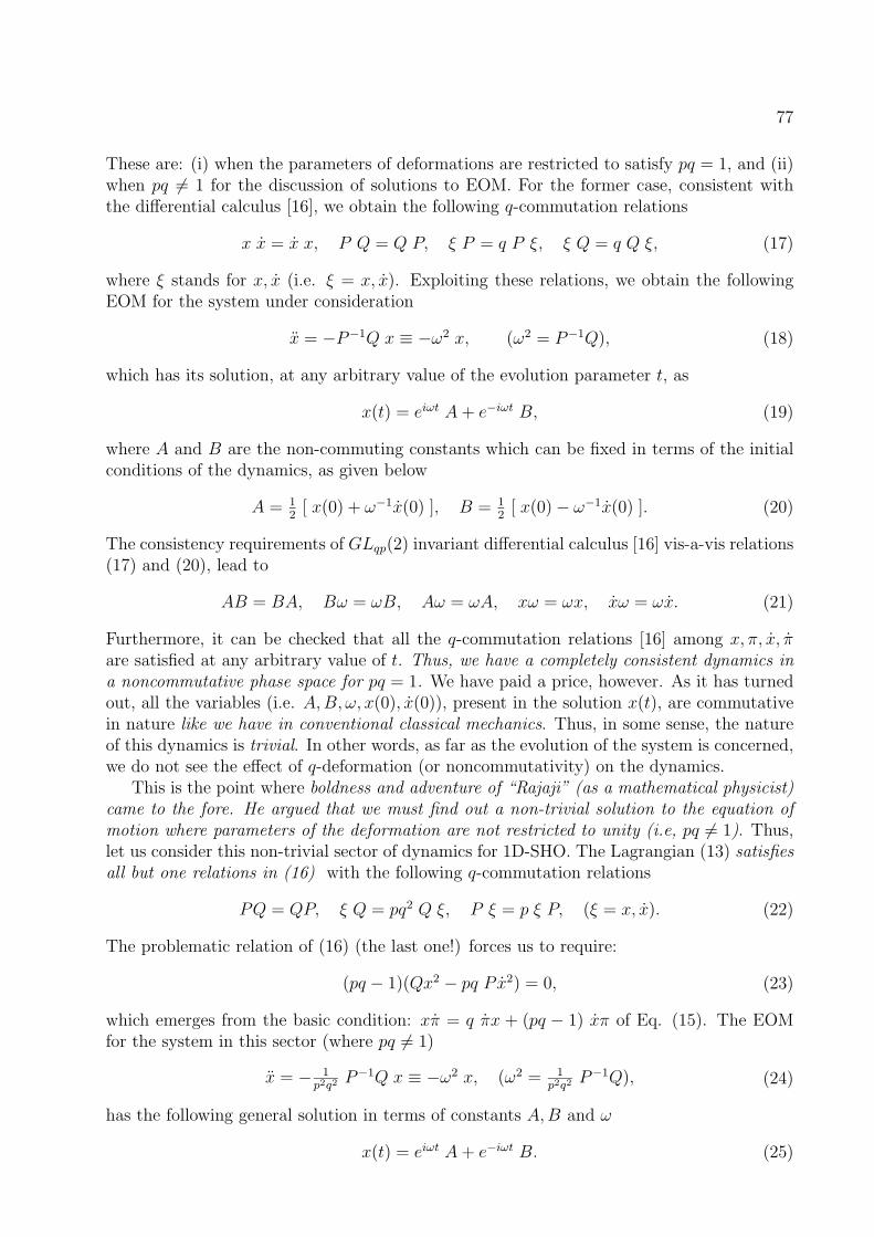
77

These are: (i) when the parameters of deformations are restricted to satisfy pq = 1, and (ii)when pq 6= 1 for the discussion of solutions to EOM. For the former case, consistent withthe differential calculus [16], we obtain the following q-commutation relations

x x = x x, P Q = Q P, ξ P = q P ξ, ξ Q = q Q ξ, (17)

where ξ stands for x, x (i.e. ξ = x, x). Exploiting these relations, we obtain the followingEOM for the system under consideration

x = −P−1Q x ≡ −ω2 x, (ω2 = P−1Q), (18)

which has its solution, at any arbitrary value of the evolution parameter t, as

x(t) = eiωt A + e−iωt B, (19)

where A and B are the non-commuting constants which can be fixed in terms of the initialconditions of the dynamics, as given below

A = 12

[ x(0) + ω−1x(0) ], B = 12

[ x(0) − ω−1x(0) ]. (20)

The consistency requirements of GLqp(2) invariant differential calculus [16] vis-a-vis relations(17) and (20), lead to

AB = BA, Bω = ωB, Aω = ωA, xω = ωx, xω = ωx. (21)

Furthermore, it can be checked that all the q-commutation relations [16] among x, π, x, πare satisfied at any arbitrary value of t. Thus, we have a completely consistent dynamics ina noncommutative phase space for pq = 1. We have paid a price, however. As it has turnedout, all the variables (i.e. A,B, ω, x(0), x(0)), present in the solution x(t), are commutativein nature like we have in conventional classical mechanics. Thus, in some sense, the natureof this dynamics is trivial. In other words, as far as the evolution of the system is concerned,we do not see the effect of q-deformation (or noncommutativity) on the dynamics.

This is the point where boldness and adventure of “Rajaji” (as a mathematical physicist)came to the fore. He argued that we must find out a non-trivial solution to the equation ofmotion where parameters of the deformation are not restricted to unity (i.e, pq 6= 1). Thus,let us consider this non-trivial sector of dynamics for 1D-SHO. The Lagrangian (13) satisfiesall but one relations in (16) with the following q-commutation relations

PQ = QP, ξ Q = pq2 Q ξ, P ξ = p ξ P, (ξ = x, x). (22)

The problematic relation of (16) (the last one!) forces us to require:

(pq − 1)(Qx2 − pq P x2) = 0, (23)

which emerges from the basic condition: xπ = q πx + (pq − 1) xπ of Eq. (15). The EOMfor the system in this sector (where pq 6= 1)

x = − 1p2q2 P−1Q x ≡ −ω2 x, (ω2 = 1

p2q2 P−1Q), (24)

has the following general solution in terms of constants A,B and ω

x(t) = eiωt A + e−iωt B. (25)

78 CHAPTER 12. QUANTUM GROUPS, Q-DYNAMICS AND RAJAJI

However, the restriction (23) is satisfied if and only if: either A = 0 or B = 0. With theexpression for A and B, given in (20), this leads to the restriction: x(0) = ± ω x(0). Nowthe general form of the exponential evolution for the 1D-SHO is either

x(t) = eiωt A, with Aω = pq ωA, (26)

or,x(t) = e−iωt B, with Bω = pq ωB. (27)

As a consequence, the dynamics for pq 6= 1 does not evolve in the 2D (velocity) phasespace but degenerates into a restricted 1D region. In this region, both the restrictions:x(t) = ± ω x(t) and Q x2 = pq P x2 are satisfied for all values of the evolution parametert. In fact, it can be checked that the evolution of the system, described by Eq. (26) and/orEq.(27), is such that these conditions are very precisely satisfied.

It will be noticed that, unlike the dynamical sector for pq = 1, here the constants ωand A (or B) do not commute with each-other and still there exists a consistent “time”evolution for the system, albeit a restricted one. In fact, as a result of the q-deformation, theevolution of the 1D-SHO is strictly on a 1D “quantum-line” even-though the whole (velocity)phase space is allowed for its evolution †. This new feature is completely different from thediscussion of a 1D-SHO in the framework of classical mechanics. It will be a nice idea todiscuss the supersymmetric version of this system in the framework of q-deformed dynamics.It will be very interesting to explore the possibility of h-deformation over q-deformation andlook for the new aspects of dynamics when q and h both are present.

†The discussion of dynamics in the cotangent (momentum phase) space has been carried out in theHamiltonian formulation as well [16].

Bibliography

[1] F. Bayen, M. Flato, C. Fronsdal, A. Lichnerowicz and D. Sternheimer, Ann. Phys. 11161, 111 (1978).

[2] U. Carow-Watamura, M. Schliecker, M. Scholl and S. Watamura, Z. Phys. C 48, 159(1990), Int. J. Mod. Phys. A 6, 3081 (1991).

[3] H. S. Snyder, Phys. Rev. 71, 38 (1947).

[4] C. N. Yang, Phys. Rev. 72, 874 (1947).

[5] H. Yukawa, Phys. Rev. 91, 415 (1953).

[6] See, e.g., for review, L. D. Faddeev, N. Reshetikhin and L. A. Takhtadjan, Alg. Anal.1, 129 (1988).

[7] See, e.g., for review, S. Majid, Int. J. Mod. Phys. A 5, 1 (1999).

[8] See, e.g., for review, A. Connes, M. R. Douglas and A. Schwarz: [hep-th/9711162].

[9] See, e.g., for review, N. Seiberg and E. Witten: [hep-th/9908142].

[10] M. Lukin, A. Stern and I. Yakushin, J. Phys. A: Math Gen 26, 5115 (1993).

[11] J. Schwenk and J. Wess, Phys. Lett. B291, 273 (1992).

[12] I. Ya. Aref’eva and I. V. Volovich, Phys. Lett. B 264, 62 (1991).

[13] R. P. Malik, Phys. Lett. B 316, 257 (1993).

[14] R. P. Malik, Phys. Lett. B 345, 131 (1995).

[15] R. P. Malik, Mod. Phys. Lett. A 11, 2871 (1996).

[16] R. P. Malik, A. K. Mishra and G. Rajasekaran, Int. J. Mod. Phys. A 13, 4759 (1998).

79

80 BIBLIOGRAPHY

Chapter 13

Geometric description of HamiltonianChaos

M.S. Sriram∗† ,

Department of Theoretical Physics, University of Madras,

Guindy Campus, Chennai 600 025, India

Introduction

Recently a geometric approach has been developed to explain the origin of chaos in Hamil-tonian systems [1, 2, 3, 4, 5]. This approach exploits the fact that the trajectories of aHamiltonian system can be viewed as geodesics on a Riemannian manifold endowed with asuitable metric.

Consider a dynamical system described by the Lagrangian

L(q, q) =1

2aik(q)qiqk − V (q), (13.1)

or equivalently the Hamiltonian,

H(p,q) =1

2aik(q)pipk + V (q). (13.2)

For a fixed energy E, define the metric tensor

gij = (E − V )aij, (13.3)

and the ’interval’ or the ’proper time’ ds by

ds2 = gijdqidqj = 2(E − V )2dt2. (13.4)

It can then be shown that the equations of motion can be written as geodesic equations ina Riemannian manifold:

d2qi

ds2+ Γi

jk

dqi

ds

dqk

ds= 0, (13.5)

∗E-mail: tphysmu@satyam.net.in†Work done in collaboration with K. Ramasubramanian, Dept. of Theoretical Physics, University of

Madras.

81

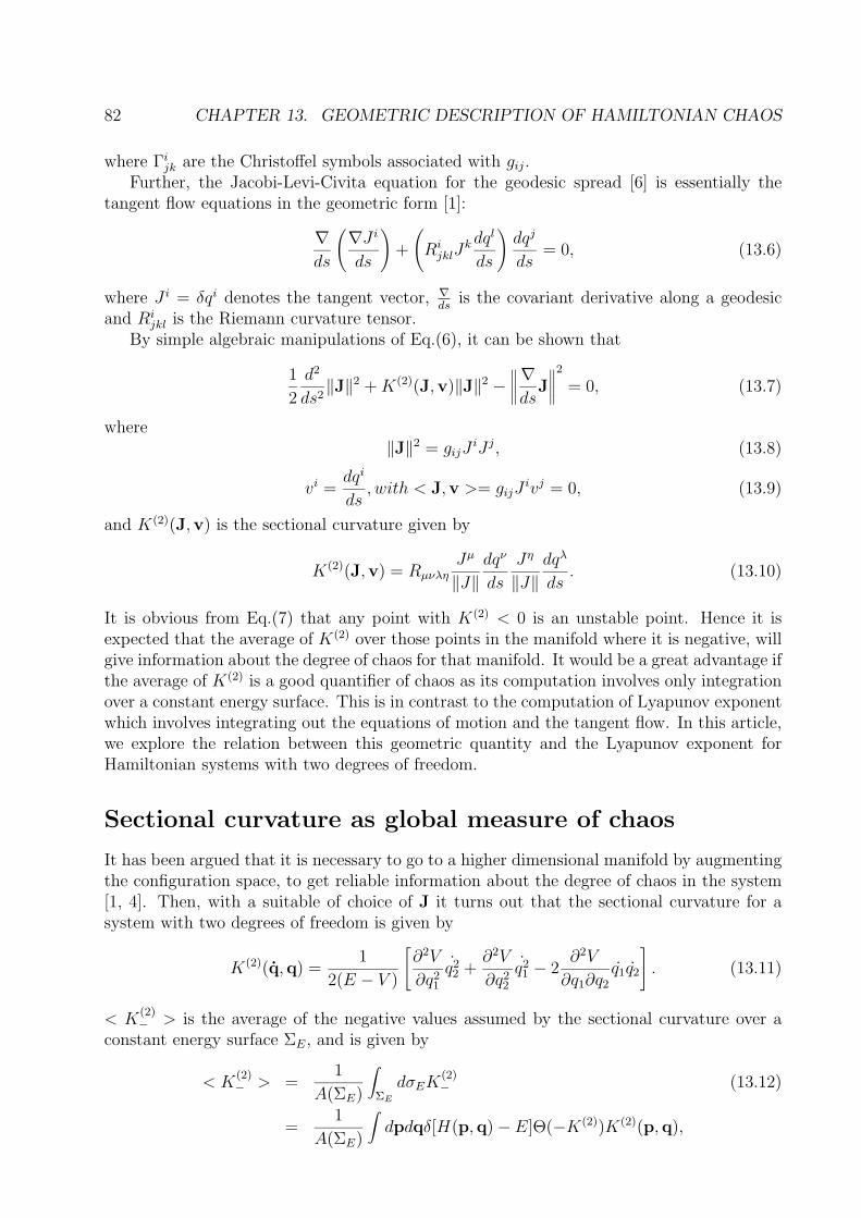
82 CHAPTER 13. GEOMETRIC DESCRIPTION OF HAMILTONIAN CHAOS

where Γijk are the Christoffel symbols associated with gij.

Further, the Jacobi-Levi-Civita equation for the geodesic spread [6] is essentially thetangent flow equations in the geometric form [1]:

∇ds

(

∇J i

ds

)

+

(

RijklJ

k dql

ds

)

dqj

ds= 0, (13.6)

where J i = δqi denotes the tangent vector, ∇ds

is the covariant derivative along a geodesicand Ri

jkl is the Riemann curvature tensor.By simple algebraic manipulations of Eq.(6), it can be shown that

1

2

d2

ds2‖J‖2 + K(2)(J,v)‖J‖2 −

∥

∥

∥

∥

∇ds

J∥

∥

∥

∥

2

= 0, (13.7)

where‖J‖2 = gijJ

iJ j, (13.8)

vi =dqi

ds, with < J,v >= gijJ

ivj = 0, (13.9)

and K(2)(J,v) is the sectional curvature given by

K(2)(J,v) = Rµνλη

Jµ

‖J‖dqν

ds

Jη

‖J‖dqλ

ds. (13.10)

It is obvious from Eq.(7) that any point with K(2) < 0 is an unstable point. Hence it isexpected that the average of K(2) over those points in the manifold where it is negative, willgive information about the degree of chaos for that manifold. It would be a great advantage ifthe average of K(2) is a good quantifier of chaos as its computation involves only integrationover a constant energy surface. This is in contrast to the computation of Lyapunov exponentwhich involves integrating out the equations of motion and the tangent flow. In this article,we explore the relation between this geometric quantity and the Lyapunov exponent forHamiltonian systems with two degrees of freedom.

Sectional curvature as global measure of chaos

It has been argued that it is necessary to go to a higher dimensional manifold by augmentingthe configuration space, to get reliable information about the degree of chaos in the system[1, 4]. Then, with a suitable of choice of J it turns out that the sectional curvature for asystem with two degrees of freedom is given by

K(2)(q,q) =1

2(E − V )

[

∂2V

∂q21

q22 +

∂2V

∂q22

q21 − 2

∂2V

∂q1∂q2

q1q2

]

. (13.11)

< K(2)− > is the average of the negative values assumed by the sectional curvature over a

constant energy surface ΣE, and is given by

< K(2)− > =

1

A(ΣE)

∫

ΣE

dσEK(2)− (13.12)

=1

A(ΣE)

∫

dpdqδ[H(p,q) − E]Θ(−K(2))K(2)(p,q),

83

where the area A(ΣE) is given by

A(ΣE) =∫

ΣE

dσE =∫

dpdqδ[H(p,q) − E], (13.13)

and Θ is the step function. This quantity < K(2)− > is the object of central interest in this

article.Stability analysis for Hamiltonians with two degrees of freedom indicates that det(∂q2V )<

0 is a sufficient condition for chaos. This is the Toda-Brumer criterion for chaos [7]. Whendet(∂2

qV ) > 0 also, chaos is possible provided there are regions in which ∂2V∂q2

1< 0 and ∂2V

∂q22

< 0.

From the expression for K(2) it can be shown that (i) det(∂2qV ) < 0 is a sufficient condi-

tion for negativity of K(2) in some regions of the constant energy manifold, and (ii) K(2) isnegative in regions with ∂2V

∂q21

< 0, ∂2V∂q2

2< 0 even when det(∂2

qV ) > 0. Hence K(2) is negative

precisely when the stability analysis indicates chaos, including the Toda-Brumer Criterion.We make a detailed comparison between < K

(2)− > and λ for the system of Coupled

quartic oscillators (CQO) whose Hamiltonian is

H =p2

1

2+

p21

2+ q4

1 + q42 + αq2

1q22, (13.14)

where α is a parameter [8]. We compute < K(2)− > and the maximal Lyapunov exponent λ for

E = 1024 and several values of α. λ is computed for 2000 random initial conditions for eachvalue of α corresponding to this energy. ¿From this, we find < λ >, the average value of theLyapunov exponent, and the fraction of phase space corresponding to chaotic trajectories, fover the 2000 initial conditions for a particular value of α. To facilitate comparison among< K

(2)− >, f and < λ >2 we plot them in the same graph against α in Fig.1. < K

(2)− > and

< λ >2 are normalized such that at α = 15, the scaled values of < K(2)− > and < λ >2 are

equal to f(= 0.904) at α = 15.

α

-0.1

0

0.1

0.2

0.3

0.4

0.5

0.6

0.7

0.8

0.9

1

0 2 4 6 8 10 12 14 16

(a) (b) (c)

Figure 13.1: Plots of (a) f , (b)-.1533 〈K(2)− 〉, and (c) 0.1012 〈λ〉2 against α.

84 CHAPTER 13. GEOMETRIC DESCRIPTION OF HAMILTONIAN CHAOS

It is remarkable that all the quantities are zero for α < 6. This follows from an analysisof the negativity of K(2) and the Toda-Brumer criterion. It is seen that < K

(2)− > is closely

related to < λ >2 rather than f . This can be understood from the scaling properties ofK(2) and λ. Under the scaling transformation, pi → β

12 pi, qi → β

14 qi, the energy scales as

E → βE and K(2) scales as K(2) → β12 K(2). Hence < K

(2)− > scales as < K

(2)− >∼ E

12

when the energy is varied. It can be shown that λ → β14 λ under the scaling transformation.

Hence λ ∼ E14 when the energy is varied. Obviously, the scaling property is valid for any

value of energy. Our numerical data confirm these scaling relations, as well as the fact thatthe fraction of phase space f corresponding to chaotic trajectories does not vary with E fora given α. This is the reason why < K

(2)− > has close correspondence with < λ >2, rather

than with f .We have considered another system known as “Yang-Mills-Higgs Hamiltonian” [9] with

H =p2

1

2+

p22

2+ 3q2

1q22 +

3

4q41 +

3

2κq4

2 −1

2κq2

2. (13.15)

Here also, it is found that < K(2)− > and < λ >2 are reasonably close to each other(apart

from a scale factor) [8]. Moreover, it is found that both < K2− > and < λ >2 scale as E

12 ,

even though the potential is not a homogeneous quartic.

Conclusions

A recently proposed geometric description of Hamiltonian chaos has been very successful,both in qualitative and quantitative aspects. For systems with a small number of degrees offreedom, it has been claimed that < K

(2)− > (a suitably defined sectional curvature averaged

over its negative values over a constant energy manifold) is an indicator of the global degreeof chaoticity at that energy. If true, this is a great advantage, as K(2) is an integral over theconstant energy surface, and one can dispense with the tedious numerical evolution of thetrajectories and the ’difference’ vector to estimate chaos in the system.

We have investigated in detail, the relations between < K(2)− >, and the average maximal

Lyapunov exponent < λ >, for some Hamiltonian systems with two degrees of freedom.We find that < K

(2)− > is closely related to < λ >2. Both < K

(2)− > and < λ >2 scale

as E12 , for the quartic potentials we have considered. In fact, for potentials which are of nth

degree in the coordinates, it is easy to see that both < K(2)− > and < λ >2 scale as E

(n−2)n .

Thus the linear relation between < K(2)− > and < λ >2 is expected to be a general feature

of Hamiltonian systems.What about systems with large number of degrees of freedom (N)? For such systems, it

has been shown that the ’global degree of chaoticity’ can be obtained by computing the meanRicci curvature, averaged over a constant energy manifold, independent of the dynamics ofthe system. It is possible to make an analytic estimate of the largest Lyapunov exponentλ, by making a Gaussian hypothesis about the statistics of curvature fluctuations along ageodesic. This exponent is in very good agreement with the corresponding exponent obtainedfrom tangent dynamics[3]. Moreover it has been demonstrated that the geometric approachcan even provide a frame work of understanding phase transition which are related to thesingular behaviour of curvature fluctuations [5]. In fact, when a system undergoes a phasetransition, the fluctuations of the configurational space curvature, when plotted as a functionof either the temperature or energy of the system exhibit a singular behaviour at the phase

85

transition point, which can be qualitatively reproduced using geometric methods.This hasbeen explicitly verified for some model large -N Hamiltonians. The success of this approachhas led Casetti, Pettini and Cohen [5] to put forth the ’Topological Hypothesis’, whoseessential content is that phase transitions would be related at a deeper level to a change inthe topology of the configuration space of the system. Hence, the geometric approach toHamiltonian dynamics has been successful in its many applications and is a promising andinteresting field of enquiry.

86 CHAPTER 13. GEOMETRIC DESCRIPTION OF HAMILTONIAN CHAOS

Bibliography

[1] M. Pettini, Phys. Rev. E 47, 828 (1993).

[2] L. Casetti and M. Pettini, Phys. Rev. E 48, 4320 (1993).

[3] L. Casetti, R. Livi and M. Pettini, Phys. Rev. Lett. 74, 375 (1995).

[4] M. Cerruti-Sola and M. Pettini, Phys. Rev. E 53, 179 (1996).

[5] L. Casetti, M. Pettini and E.G.D. Cohen, Phys. Rep. 337, 237 (2000).

[6] T. Levi-Civita, Ann. Math. 97, 291 (1926).

[7] M. Toda, Phys. Lett. A 48, 335 (1974); P. Brumer and W. Duff, J. Chem. Phys. 65,3566 (1976).

[8] K. Ramasubramanian and M.S. Sriram, Global geometric indicator of chaos and Lya-punov exponents in Hamiltonian systems, Phys. Rev. E, to be published.

[9] T. Kawabe, Phys. Lett. B 274, 399 (1992).

87

88 BIBLIOGRAPHY

Chapter 14

Quantum dynamics of superposed

states and classical nonlinear maps

S. Lakshmibala and M.V. Satyanarayana

Department of Physics, Indian Institute of Technology,

Chennai 600 036, India

Introduction

The phase space dynamics of classical systems whose evolution is governed by nonlinearequations has been studied extensively for over several years now. The long-time behaviourof such systems and the degree of randomness they exhibit varying from mere ergodicity tochaos have been analysed extensively using both analytical and numerical tools. While muchinvestigation has been undertaken on low-dimensional maps and flows, and the classical dy-namics that arises in the phase space of these systems examined, their quantum counterpartshave not been investigated in great detail. While in broad terms, chaos in classical systemscan be traced back to the nonlinear equations that govern the system’s temporal evolution,the quantum counterparts obey the Schrodinger equation, (or the Liouville equation, formixed states). These are linear equations, and information loss in these systems must arisefrom repeated measurements and the effects of the uncertainty principle. But the precisemanner in which such information loss arises is poorly understood, and needs further study.

One aspect of such a study is the identification of suitable quantum systems where thediscrete time evolution of an appropriate parameter is guided by a classical nonlinear mapequation. Such an example of a quantum phenomenon arises in the context of wave packetrevivals, where the dynamics of an appropriate phase is identical to the classical rotationmap on the circle [1]. This map exhibits ergodicity, and not chaos. An obvious extensionthen would be the identification of a quantum system where the underlying dynamics of anappropriate phase exhibits full-fledged chaos. The temporal dynamics of such a phase wouldbe given by a chaotic one-dimensional map, like the Bernoulli shift map. The shift map notmerely serves as a paradigm of chaos, but also displays the ultimate stage in the hierarchyof randomness. In fact, in a certain sense, the Bernoulli shift is as random as a coin toss. Itis therefore a matter of considerable interest to identify quantum mechanical analogs of thismap. We have examined such a case, namely, the quantum cloning of the photon, an examplewhich gets more impetus due to the fact that it is the optical analog of the quantum network

89

90 CHAPTER 14. QUANTUM DYNAMICS OF SUPERPOSED

given for relative phase estimation [2]. We outline the essential features of both the wavepacket revival phenomenon and the cloning problem in the subsequent sections. These twoexamples have been selected as they display both the extreme situations in the hierarchy ofrandomness that arises in nonlinear dynamics - namely, mere ergodicity and fully developedchaos. In the next section we review the problem of wave packet revivals, and in Section3 we examine the evolution of a suitable phase, in repeated cloning of the photon throughstimulated emission from two-level atoms.

Wave Packet Revivals

Revivals of a non-stationary state of a Hamiltonian may be regarded as the quantum analogsof recurrences in a classical dynamical system. In general, when a quantum mechanicalsystem is in a state |ψ〉, the autocorrelation function |〈ψ(0)|ψ(t)〉|2 decays from its initialvalue of unity as the time t increases. Under very specific conditions however, it may returnto its initial value at certain instants of time, signalling a full revival. In the generic casethough, any return would be to a value in a small neighborhood of unity [3], which weshall term a “near revival”. This would be the counterpart of a Poincare recurrence [4] ina classical system, although, of course, there is no direct connection between revivals andclassical periodic orbits in the phase space of the same physical system. Due to the fact thatmeasuring devices have a non-zero least count, in practice near revivals rather than exactrevivals are the readily identifiable phenomena of interest.

In a system whose evolution is governed by a nonlinear Hamiltonian, both revivals andfractional revivals can occur. Fractional revivals correspond to a situation where the wavepacket evolves to a superposition of similar wave packets. Both revivals and fractionalrevivals of wave packets are of considerable current interest in many contexts, for example,in atom optics [5], propagation of coherent light through a Kerr medium [6], the dynamicsof population inversion of atoms interacting with radiation [3, 7, 8] etc.

Our interest here is in near revivals. It is possible to suitably cycle the parameters in thegoverning Hamiltonian to suppress fractional revivals [9]. This is because as a by-productof the cyclic variation of the parameters in the Hamiltonian, the state vector may pick upan extra geometric phase . This phase can be exploited to get rid of fractional revivals.Once fractional revivals are suppressed the system can be effectively modelled by a linearHamiltonian which allows for full or near revivals alone to occur. Further, the introductionof a time period T over which the parameters are cycled, also discretizes time in a naturalway, and it is only at instants separated by an interval T that the Hamiltonian returns toits original self. We therefore look for revivals of a state only at the instants T, 2T, · · ·.Correspondingly, we analyze the problem in terms of returns in a discrete-time map. Dueto the presence of the geometric phase the revival times get shifted by the time required tocover the angular excess (or decrement) representing the anholonomy in the semiclassicallimit, namely, the corresponding Hannay angle [10].

For definiteness, we demonstrate this in the case of a unitarily deformed oscillator Hamil-tonian whose eigenstates are generalized coherent states, while the spectrum remains linear(equi-spaced). These states provide a setting in which anholonomies can be measured ex-perimentally [11, 12] and analyzed theoretically [13, 14], in a physical range extending fromthe extreme quantum regime to the semiclassical limit. The latter can thus serve as a clearsignature of the dynamics of wave packet revivals. In what follows therefore, we discuss therevival problem with special emphasis on the oscillator coherent states.

91

Consider a system with a time-independent hermitian Hamiltonian H, with spectrum{En} and eigenstates {|φn〉}. Let the system be prepared in an initial state |ψ(0)〉 that is asuperposition of the {|φn〉}, sharply peaked about some n0. We expand En as

En = En0 + (n − n0) E ′n0

+ (1/2)(n − n0)2 E

′′

n0+ · · · (14.1)

As we wish to analyze only revivals and fractional revivals, we retain only terms up to thesecond order in Eq. (14.1) and by suitably shifting n we have the quadratic form

En = C0 + C1 n + C2 n2 . (14.2)

The coefficients Ci evidently depend on the parameters that occur in H. We shall assume,without loss of generality that C1, C2 > 0. In the |φn〉-basis the time evolution operatorU(t) = exp [−i H t/h] has the representation

U(t) =∞∑

n

exp[−i (C0 + C1 n + C2 n2)t/h]|φn〉〈φn |. (14.3)

For a full revival (the auto-correlation function C(t) = 1) to occur at time t, U(t) mustreduce to the unit operator (apart from a possible overall phase factor), i.e., (C1n + C2n

2)tmust be an integer multiple of 2πh for every n in the summation. The following cases arise:

(i) C1 6= 0, C2 = 0 (equi-spaced or linear spectrum): Revivals of an initial state occurwith a period Trev = 2πh/C1.(ii) C1 = 0, C2 6= 0: Revivals occur with a period Trev = 2πh/C2.(iii) C1, C2 6= 0, C1/C2 = a rational number r/s: Once again, full revivals occur with afundamental revival time Trev = 2πhs/C2. A specific example is provided by the Hamiltonian

a†2a2 = a†a(a†a − 1) that is relevant to wave packets propagating in a Kerr medium. It isevident that, in this case, En is proportional to n(n − 1) which is an even integer for everyn.(iv) C1, C2 6= 0, C1/C2 irrational (the generic case): As the condition (C2n

2+C1n)t = 2πhm(m = integer) cannot be satisfied for all n at any value of t, full revivals are no longer possible.However, at certain instants of time the quantity C(t) could come arbitrarily close to unity,producing a near revival.

Between occurrences of full (or near) revivals, the wave packet breaks up into a finitesum of subsidiary packets at specific instants of time, provided the spectrum is nonlinear,i.e., C2 6= 0 [15]. These fractional revivals occur at times t given by t = πhr/C2 s wherer and s are mutually prime integers. It can be shown that at these instants the evolutionoperator U can be expressed as a finite sum of operators Up, in each of which the phasefactor multiplying the projection operator |φn〉 〈φn| is linear in n: That is,

U (πhr/C2 s) =l−1∑

p=0

a(r,s)p Up , (14.4)

with

a(r,s)p = (1/l)

l−1∑

k=0

exp[

−(i π k2r/s) + (2 i π kp/l)]

, (14.5)

and

Up =∞∑

n=0

exp (−i nθp) |φn〉 〈φn| , θp = π [(C1r/C2 s) + (2p/l)] . (14.6)

92 CHAPTER 14. QUANTUM DYNAMICS OF SUPERPOSED

It is this decomposition of U which is responsible for fractional revivals, as can be seen byexamining the action of the operator Up on the initial state. For instance, if the initial state|ψ(0)〉 is the “coherent state” |z〉 given by

|z〉 = exp(

−|z|2/2)

∞∑

n=0

zn

√n!

|φn〉 , z ∈ C , (14.7)

Eqs. (14.4)–(14.6) yield

|ψ(πhr/C2s)〉 = exp (−iπC0r/C2 s)l−1∑

p=0

a(r,s)p |z exp(−i θp)〉 . (14.8)

The state at time πhr/C2s is therefore a weighted sum of wave packets, each of which hasthe same form as the initial state |z〉.

It is clear from the foregoing that fractional revivals arise from the quadratic dependenceof En on n, and further, a whole host of such revivals of varying intensities can appear in agiven case, depending on the precise values of C2 and the integers r and s for which theserevivals are detectable. However, by inducing suitable geometric phases in the basis states|φn〉, we can eliminate these partial revivals and restore near revivals at specific instants oftime.

To demonstrate this, we now consider the situation in which the Hamiltonian contains aset of “slow” parameters R that can be varied adiabatically and cyclically with period T , asin Berry’s original setting for the geometric phase: i.e., RT = R0. For a general nonlinearspectrum En, one may expect that the dependence of the geometric phases on n is of theform

γn = Θ0 + Θ1 n + Θ2 n2 + · · · (14.9)

This is generic, as it only requires that γn be a regular function of n. As in the expansion ofEn, only terms up to O(n2) in the above equation are relevant for our present purposes. Thecoefficients Θi will clearly depend on the manner in which the parameters R are varied. Theunitary operator responsible for the time evolution of the wave packet will now get modifiedto

U(kT ) =∑

n

exp[

i k(ν0 + ν1n + ν2n2)

]

|φn ,R0〉 〈φn,R0| (14.10)

where

νi = Θi − (1/h)∫ T

0Ci(t) dt , (i = 0, 1, 2) . (14.11)

From the earlier discussion, it is clear that all fractional revivals of a wave packet will beeliminated if the coefficient ν2 of n2 in the foregoing expression for U(kT ) vanishes: thishappens if we arrange the variation of the parameters such that Θ2 = (1/h)

∫ T0 C2(t) dt .

Once this is done, the exponent in U(kT ) has only terms that are linear in n. Hence, at therelevant times kT (k = 1, 2, · · ·), the wave packet will no longer exhibit fractional revivals.

After the cancellation of the n2 term in the phase factors in Eq. (14.10), the effectivetime development operator at time kT (k = 1, 2, · · ·) is of the form

U(kT ) = exp(ikν0)∑

n

exp(iknν1) |φn ,R0〉 〈φn,R0| . (14.12)

Therefore an initial coherent state |ψ(0)〉 = |z〉 given by Eq. (14.7) evolves to

|ψ(kT )〉 = |z exp(ikν1)〉 . (14.13)

93

Correspondingly, the autocorrelation function becomes

C(kT ) = exp[

2|z|2 (cos kν1 − 1)]

. (14.14)

Thus, if kν1 happens to be an integer multiple of 2π (recall that ν1 depends on T ), thenfull revivals occur with Trev = kT as the basic revival time. In general, however, ν1 isan irrational number (modulo 2π). Therefore, if θ0 is the phase of the complex number zlabelling the initial state |ψ(0)〉, and θk that of the corresponding number at time kT , Eq.(14.13) shows that the discrete time evolution of the state is entirely equivalent to the circlemap

θk = θk−1 + ν1 (mod 2π) (14.15)

corresponding to a rotation.Equivalently, we can write

θk+1 = θk − 2π∆ (mod 2π). (14.16)

If ∆ is a rational number p/q, every orbit of the map is periodic with a period q. Corre-spondingly, every initial state |z(0)〉 has revivals at times qT, 2qT, · · · .

The generic case however, corresponds to an irrational value of ∆. As is well known, themap no longer has any periodic orbits, but the iterates of any θ0 cover S1 densely as k → ∞.The dynamics is ergodic but not mixing, with a uniform invariant density ρ(θ) = 1/(2π).Although we no longer have exact revivals in principle, the system exhibits near revivals –precisely the analog of Poincare recurrences. Hence, the following complete analysis of thestatistics of near revivals can be done.

Consider a prescribed small angular interval Iε of size 2πε, located symetrically aboutthe initial phase θ0 on S1. Let ∆ ≡ [∆] + δ, where [∆] stands for the integer defined by∆−1 < [∆] < ∆ (for either sign of ∆), so that δ is an irrational number satisfying 0 < δ < 1.It is then easy to see that θk ∈ Iε ⇒ {kδ} < ε, where {x} denotes the fractional part of x andthe corresponding correlation function then merely differs from unity by a term of order ε2.To order ε, therefore, we may regard a return of θk to Iε as a (near) revival. The statisticsof the occurrence times of such revivals is then identical to that of the recurrences to anangular interval of size 2πε in the rotation map. The solution to the latter problem is givenby certain gap theorems for interval exchange transformations [16, 17]. Applying these tothe case at hand, we obtain the following results in the long-time limit, after the transientsdue to specific initial conditions have died out and the invariant measure is attained. Themean time between successive near revivals is, in units of T , the reciprocal of the invariantmeasure of Iε and is just T/ε, as one may expect. The distribution of recurrence times is,however, quite remarkable [18]. In general (i.e., for arbitrary ε and δ), it is concentrated atno more than three points T1 = k1T, T2 = k2T and T3 = T1 + T2, where k1 and k2 are theleast positive integers such that

{k1δ} < ε and 1 − {k2δ} < ε (14.17)

respectively. (Recall that ε ¿ 1; as long as ε < 1/2, k1 6= k2.) It is easy to show thatε ≤ {k1δ} + 1 − {k2δ}: when the equality sign applies, only two recurrence times (T1 andT2) occur.

We have considered the example of wave packet revivals where the phase in questionevolves like the map variable of the rotation map, which is not chaotic. and demonstrated

94 CHAPTER 14. QUANTUM DYNAMICS OF SUPERPOSED

how results from ergodicity theory can be used to make predictions on revival times. In thenext section, we discuss another example from quantum mechanics, namely photon cloningthrough light-atom interactions. We identify a phase in this problem which evolves in discretetime like the map variable corresponding to the Bernoulli shift map.

Quantum Cloning

Photon cloning has had a rich history. When a two-level atom in the excited state releases aphoton through stimulated emission due to interaction with an incident photon, the emittedphoton is guaranteed to have the same polarization as the incident photon. In this sense, aperfect copy of the incident photon has been produced. In their seminal paper [19] Woottersand Zurek argue that given such a quantum cloning machine that ideally copies some po-larization states, arbitrary quantum superpositions of these states cannot be exactly cloned.However,the extent to which these superposed states can be cloned have been examined andquantifiers of the efficiency of cloning have been given both in terms of the Hilbert-Schmidtnorm of the difference between appropriate density matrices [20], and a suitably definedfidelity factor [21]. In turn, both input state-dependent and universal quantum copying ma-chines have been proposed, and their designs have been suggested [22] using both logic gatesand optical devices.

However, one aspect which is not examined here is the nature of information loss inthe relstive phase between superpositions of basis states when the bases are ideally clonedrepeatedly in a copying machine. The standard prescription to determine the relative phasebetween two beams of light into which an initial beam is split, is to conduct an interferenceexperiment. This has a parallel in a very different area - namely, quantum networks andinformation theory, where a set-up has been given to estimate the relative phase between twoqubits [2]. Inspiration for this set-up can be traced back to the two fundamental propertiesof quantum states- superposition and interference. These two principles have also playeda major role in other related areas of quantum information theory like the development ofrapid search algorithms in a given database, algorithms for drastically reducing the numberof computational steps in a given problem, and so on. Dividing information which wasoriginally contained in a single bit into a superposition of qubits, is achieved in networktheory through an Hadamard transformation. This is the analog of what a beam-splitterdoes in conventional optics. The relative phase between two qubits itself is determined in thecontext of networks by using appropriate X-OR gates. A suitable combination of Hadamardtransformations and the X-OR operation is the analog of an interference experiment in opticsconducted to determine the relative phase between two states.

It is a matter of interest that a similar combination has been successfully suggested tosolve the problem posed by Deutch [23], concerning Boolean functions. Here, one is requiredto determine in a single measurement whether a given function is a constant or a balancedfunction, where, in general there are four options, two corresponding to constant functionsand two to balanced functions. The procedure has been successfully extended to solve a moregeneralized version of the Deutsch problem subsequently proposed by Deutsh and Jozsa [24].

Returning to the problem at hand, namely, relative phase estimation, we first brieflyreview the essential features of the network proposed to estimate the relative phase betweentwo qubits. This is based on the theory of quantum Fourier transforms [25], and we outlinethe pertinent features below: Let a ε {0.1}m. a is a thus a binary string with m entries, eachbeing 0 or 1. In decimal notation, a ε {0, 1, 2, ......2m − 1}. The quantum Fourier transform

95

on the additive group of integers modulo 2m is a mapping done on a and is defined as [2]

|a〉 →2m−1∑

y=0

exp(2πiay/2m)|y > . (14.18)

Here, y ε {0, 1, 2, .....2m − 1} and |a〉 has m entries, each being 0 or 1. In binary notation,the above equation reads as

|a〉 →2m−1∑

y=0

exp(2πi(0.a1a2a3....am)y)|y > . (14.19)

This follows from the fact that if a = (a1a2a3...am), where each of the aks takes on the value0 or 1, and k = (1, 2, ...m), a/2m = (0.a1a2a3...am). It can then be checked that for a givenvalue of |y〉 say |y1y2y3...ym〉, exp(2πi(0.a1a2a3...am)(y1y2y3...ym))|y1y2y3...ym〉 can again bewritten as the product

exp(2πi(0.am)y1)|y1〉 exp(2πi(0.am−1am)y2)|y2〉...exp(2πi(0.a1a2a3...am)ym)|ym〉 .

In the above we have omitted the integral part of (a)(y). It can also be independently verifiedthat the RHS of Eq.(14.18) can be factorized in the form

(|0〉+exp(2πi(0.am))|1〉) (|0〉+exp(2πi(0.am−1am))|1〉) ...(|0〉+exp(2πi(0.a1a2a3...am))|1〉) .

and that each term tnat arises here can be identified with a corresponding term in the productform given earlier. In this sense the quantum Fourier transform of |a〉 is factorizable.

Good estimators for arbitrary phase differences between states can be obtained using theprinciple of the quantum Fourier transform outlined above. We briefly discuss a procedurefor doing this using networks, and subsequently draw parallels between this procedure and aphoton cloning experiment that we will outline. Further, in both cases we will indicate howan appropriate relative phase exhibits chaos. The network for estimatimg relative phasesrelies on the implementation of a set of n unitary transformations U2n on qubits. Let |ψ〉 bean eigenvector of U2n such that

U2n |ψ〉 = exp(2πi2nφ)|ψ〉 . (14.20)

Here, 0 ≤ φ ≤ 2π. Apart from the state |ψ〉 a ‘control’ qubit is also provided. U2n iscalled a ‘controlled’ unitary operator as it’s action is such that if the control qubit is in thestate |0〉, it performs the identity operation on |ψ〉, and it pulls out a factor exp(2πi2nφ), ifthe control qubit is in the state |1〉. These are the only two states allowed for the controlqubit. Thus we have,

U2n |0〉|ψ〉 → |0〉|ψ〉, (14.21)

andU2n |1〉|ψ〉 → exp(2πi2nφ)|1〉|ψ〉 . (14.22)

Clearly, the controlled unitary operation mimics the X-OR operation in logic gates as itintroduces a relative phase between the two states |0〉 and |1〉.

We now discuss the actual network [2]. It initially consists of an auxiliary qubit |ψ〉and n qubits, each prepared in the state |0〉. We shall label these n qubits |0〉i, with i =0, 1, 2, ...n − 1. An Hadamard transformation is now done on the |0〉is, so that each splits

96 CHAPTER 14. QUANTUM DYNAMICS OF SUPERPOSED

up to a superposition of (|0〉 + |1〉), apart from the normalization. The operation U20 isnow performed on |0〉0|ψ〉. This leaves |ψ〉 unchanged and converts |0〉 − 0 to |φ〉0 which is(|0〉 + exp(2πi20φ)|1〉). This is followed by the operation U21 on |ψ〉 and |0〉1. The operationclearly converts them to the output state |ψ〉 and |φ〉1 which is simply (|0〉 + exp(2πi21φ)|1〉).In the next stage, the operation U22 is carried out on the pair |ψ〉 and |0〉3, and so on. Thereare totally n stages in this operation and the net output clearly consists of the auxiliaryqubit |ψ〉 tigether with the set |φ〉i with i = 0, 1, 2, .n − 1. This set can be writtenas

∑2m−1y=0 exp(2πiφy)|y〉. From our earlier discussion it is evident that the network has

implemented a quantum Fourier transform on |φ〉. However, φ is not in general a rationalnumber, and only an m-bit estimate of φ can be obtained by doing the inverse quantumFouries transform of the above output.

Now consider a realistic situation, where the network above is slightly modified, as follows:We begin the discussion at that stage when the first unitary transformation has been alreadyimplemented and |0〉0 has been converted to |φ〉0. Let us suppose that the phase φ is measuredwith a suitable device, and the measured value is used as an input in the first stage of theprogram- namely, in implementing the unitary transformation U21 on the appropriate states.The generic φ, being irrational, an initial error has already been introduced in implementingU21 . If the new phase is measured and used to implement U22 in the second stage thiserror magnifies. At the end of n steps of the program, a small error ε in the initial phasemeasurement has increased to 2nε. In fact the phase φ is governed by the map equation

φn+1 = 2φn, (14.23)

where the suffix denotes the stage in the operation, and φ is considered modulo 2π. Theinitial error ε in the measurement of φ is also governed by a similar equation. This is simplythe map equation for the Bernoulli shift map, which displays chaos and has a Lyapunovexponent equal to ln 2.

We now return to the photon cloning experiment we mentioned earlier and examine thepossibility of finding the equivalent of the network problem in optics, replacing the Hadamardoperation and the X-OR gates with coherent states, beam splitters, light-atom interactionsthrough stimulated emission and an interference experiment. We denotee the initial state ofthe radiation field in the experiment that we outline below, by the standard coherent state |z〉given in Eq.(14.7).Other states of the radiation field that arise during the cloning procedurewill be described by appropriate superpositions of |z〉 and the genaralized coherent states{|n, z〉}, with n = 1, 2, ...The generalized coherent states are got by repeated application ofthe operator(a† − z∗) on |z〉. The set {|z〉, |n, z〉} form an orthonormal basis. In contrastto these states the photon-added coherent states {|z, n〉}, with n = 1, 2, ... [26], do notform an orthonormal set, and can in fact be expanded in the basis given above. In general,normalizing them to unity, we have

|z, n〉 = c0|z〉 +n

∑

p=1

cp|p, z〉 , (14.24)

with the cis i = 0, 1, .. being the expansion coefficients whose modulus2 sums up to unity.To begin with, we consider the interaction of the radiation field |z〉 with two-level atoms

in the excited state. The set-up requires the suppression of spontaneous emission of photons,so that ideal cloning can occur. A single photon in this radiation field interacts with onetwo-level atom and produces a clone of itself. Consequently the state of the radiation field

97

changes to the one-photon added coherent state |z, 1〉 [26]. The relative phase χ0 between|z〉 and |z, 1〉 is given by

χ0 = (1/i) ln (< z|z.1 >

| < z|z, 1 > |) (14.25)

with 0 ≤ χ0 ≤ 2π. In the first stage of the operation that follows this, the cloned photonproduces another copy of itself through stimulated emission of another excited two-levelatom. Consequently, the radiation field transforms to |z, 2〉. The relative phase between |z〉and |z, 2〉 is now χ1 given by

χ1 = (1/i) ln (< z|z.2 >

| < z|z, 2 > |) (14.26)

This can be simplified using the fact that |z, 2〉 is obtained by applying a† twice on |z〉, andwe get

χ1 = 21χ0. (14.27)

In the second stage of the cloning program, each of the two photons produces a copy ofitself by inteaction with two excited atoms, and therefore the radiation field is described by|z, 4〉. The relative phase between this and |z〉 can be seen to be 22χ0. At the nth stage ofthis cloning progra, the corresponding relative phase χn satisfies

χn = 2nχ0 (14.28)

modulo 2π. This is identical to the manner in which the phase φ evolved in the networkproblem discussed earlier, and again the equation can be mapped on to the equation govern-ing the map variable in the shift map. A small error in the estimation of the initial relativephase, magnifies exponentially, and the system displays extreme sensitivity to the initialvalue of the phase. To that extent the prediction of the relative phase, after many stages ofthe cloning program becomes meaningless.

We have outlined above the optical analog of the network that determines relative phases.An interesting problem that arises in this context is the generalization of this cloning programto include other classes of coherent states, and obtaining a quantum analog of the shift mapin terms of operators. The results of this study will be reported elsewhere.

Acknowledgment : We take great pleasure in submitting this article to the Proceedingsbrought out in honour of Prof.G. Rajasekaran.

98 CHAPTER 14. QUANTUM DYNAMICS OF SUPERPOSED

Bibliography

[1] S. Seshadri, S. Lakshmibala and V. Balakrishnan, Phys. Lett. A 256, 15 (1999).

[2] R. Cleve, A. Ekert, C. Macchiavello and M. Mosca, Proc. Roy. Soc. (London) A454,339 (1998).

[3] J. H. Eberly, N. B. Narozhny, and J. J. Sanchez-Mondragon, Phys. Rev. Lett. 44, 1323(1980).

[4] M. Kac, Probability and Related Topics in Physical Sciences (Interscience, New York,1959).

[5] G. Rempe, H. Walther, and N. Klein, Phys. Rev. Lett. 58, 353 (1987).

[6] K. Tara, G. S. Agarwal, and S. Chaturvedi, Phys. Rev. A 47, 5024 (1993).

[7] M. V. Satyanarayana, P. Rice, R. Vyas, and H. J. Carmichael, J. Opt. Soc. Am. B 6,228 (1989).

[8] J. I. Cirac, R. Blatt, A. S. Parkins, and P. Zoller, Phys. Rev. A 49, 1202 (1994).

[9] S.Seshadri, S. Lakshmibala and V. Balakrishnan, J. Stat. Phys.101, 213 (2000).

[10] C. Jarzynski, Phys. Rev. Lett. 74, 1264 (1995).

[11] R.Y. Chiao and Y.S. Wu, Phys. Rev. Lett. 57, 933 (1986); A. Tomita and R.Y. Chiao,ibid. 57, 937 (1986); n.R. Bhandari and J. Samuel, ibid. 60, 1214 (1988); M. Seger, R. Solomon, and Y. Yariv,ibid. 69, 590 (1992).

[12] P. Hariharan and P.E. Ciddor, Opt. Comm. 110, 13 (1994); P. Hariharan, G. Kieran,G. Larkin, and M. Roy, J. Mod. Opt. 41, 663 (1994); P. Hariharan and M. Roy, ibid.41, 2197 (1994).

[13] S. Chaturvedi, M.S. Sriram, and V. Srinivasan, J. Phys. A 20, L1071 (1987).

[14] S. Seshadri, S. Lakshmibala, and V. Balakrishnan, Phys. Rev. A 55, 869 (1997).

[15] I. Sh. Averbukh and N. F. Perelman, Phys. Lett. A 139, 449 (1989).

[16] G. Rauzy, Acta Arithmetica 34, 315 (1979).

[17] N. B. Slater, Proc. Camb. Phil. Soc. 63, 1115 (1967).

99

100 BIBLIOGRAPHY

[18] The same distribution manifests itself in recurrences to any cell when quasiperiodic flowon a two-torus is coarse-grained. See C. Nicolis, G. Nicolis, V. Balakrishnan, and M.Theunissen, in Stochastic Dynamics, ed. L. Schimansky-Geier and T. Poschel (Springer-Verlag, Berlin, 1997), pp. 42-54; M. Theunissen, C. Nicolis, and G. Nicolis, J. Stat. Phys.94, 437 (1999).

[19] W.K. Wootters and W.H. Zurek, Nature (London) 299, (1982) 802.

[20] V.Buzek and M. Hillery, Phys. Rev.A 54, 1844 (1996).

[21] B.Schumacher, Phys. Rev. A 51 2738 (1995).

[22] M.Gisin and S. Massar, Phys. Rev. Lett. 79, 2153 (1997).

[23] D.Deutsch, Proc. Roy. Soc. (London) A 400, 97 (1985).

[24] D.Deutsch and Jozsa, Proc. Roy. Soc. (London) A 439, 553 (1992).

[25] D.Coppersmith, IBM Research Report No. RC19642.

[26] G.S.Agarwal and K.Tara, Phys. Rev.A 43, 492 (1991).

Chapter 15

Felicitations

Several colleagues and friends of Rajaji who could not participate in the Rajaji Symposiumsent messages wishing him well on his 65th birthday. We have reproduced some of the moredetailed ones below.–Eds.

From Prof. R.H. Dalitz

I am sending this e-mail message∗ to congratulate you on reaching your 65th birthday andon your excellent record of academic work, whether we consider your research or your ad-ministrative work in the Institute of Mathematical Sciences at Chennai. I believe that youare also reaching your retirement age now, although I do not know whether it takes place onthe date of this birthday or whether it will be delayed until the end of this Academic Year.Either way, I wish you a happy retirement!

I met you first at the Summer School which the Tata Institute for Fundamental Researchat Bombay (now Mumbai) had organised to take place at Bangalore in 1961. I don’t remem-ber when it was that you came to Chicago University to work in the Enrico Fermi Instituteof Nuclear Studies as a graduate student there. We must have got off with a quick start,since our first joint paper, on spins and lifetimes of light hypernuclei, was published in thefirst issue of Phys. Lett., dated 1962. Most likely, you arrived in Chicago in the Fall of 1961.The work you did in the years 1961-63 was a mixture of hypernuclear physics and strangeresonance physics. I recall that your Ph.D. dissertation was a rebuttal of the Yang/Oakespaper which said “that the large mass differences between particles in different channels forthe resonance meant that SU(3) symmetry could not hold. It must be wrong”. What youproved in your Ph.D. thesis was that this conclusion was not necessarily so.

I visited Chicago for the KAON99 conference. One of the gentlemen just mentionedabove, came over to me at this Conference and happened to say that he had not understoodwhat mistake they had made until he had read your Ph.D. thesis. They haven’t forgottenyou there, Raja.!

I remember also the case of a multichannel system, with energy thresholds at . . . i, i +1, i + 2, . . ., so that there are many thresholds. We realised that there were many ways toleave the Energy-plane, e.g., crossing over the real axis between threshold i and (i + 1) orthat between (i + 1) and (i + 2), each getting onto a different unphysical sheet. However

∗Prof. Dalitz sent this e-mail message with a request that it “be read at the celebration of ProfessorRajasekaran’s 65th birthday”.

101

102 CHAPTER 15. FELICITATIONS

there was a resonance pole on both unphysical sheets, indeed one for each of these unphysicalsheets. They are now known as “shadow poles”. We didn’t invent that name, but it is avery evocative name.

Well, we had quite a lot of fun with other questions, calculations about the 1405 MeVresonance in the hyperon-meson system—its nature is still an open question—and we madethe first determination of the strength of the Lambda-Nucleon force, much weaker than theNucleon-Nucleon force.

I think that you came with me to Oxford in 1963/4, where you worked on your thesis,before you went back to Chicago for your Ph.D. examination. We had a good time in thosedays. Life doesn’t stop when you become “retired”. I wish you a happy retirement and thatyou will find enjoyable and creative things to do.

Dick Dalitz,Oxford University,

U.K.

From R.K. Bhaduri

The stage must be all set, after all the preparations and planning, for this meeting honouringRajasekaran’s contributions to physics research and development. It is too bad that I cannotbe present Before conveying my regards to him, I cannot resist here to reminesence, perhapsnot very accurately, some incidents during our long friendship.

In 1959, when I joined TIFR, Rajasekaran was already there. But at that time I did notknow him too well. I remember him vividly in the Christmas Party of 1963 that Professorand Mrs. Peierls used to throw every year at 12 Parks road, Oxford. Rajasekaran wascompleting his Ph.D. with Dalitz. At the party, he was standing by the staircase near theentrance with a glass full of wine. My wife and I were already good friends of his by thattime. As a good friend, I had to help him empty the wine glass before Mrs. Peierls camewith more ! Next summer, in 1964, he finished writing his thesis (I recall it had to do withOmega− and SU(3)), and decided to come with us to Europe on a short vacation. He insistedon bringing the manuscript of his thesis with him, so that it does not get lost in his absence.While boating on Lake Como, we threatened to drop it in the lake unless he treated us ina restaurant in Paris. Rajaji good-naturedly agreed, and so we had a grand celebration forhis Ph.D. much before it was awarded. During this time, Divakaran and Rajasekaran usedto visit our home frequently, and we have nice memories of many evenings spent together.

In 1967, when I went back to TIFR, Rajasekaran was a prominent member of the theorygroup. I recall he was still interested in ΛHe3 life-time, where there was confusion thatcould be blamed on some wrong experiments. Rajasekaran was always a very clear-thinkingperson, with a quick grasp. I think I would have collaborated with him, but for the factthat I left soon. I remember that at this time he was already married, with a very youngand beautiful wife, Swatantra, who cooked fabulous dinners. Much later, I wanted to spendmy sabbatical in Madras (in 1981), with the intention of learning QCD (I still want to).Rajasekaran had done some very good work on weak interactions too in the seventies atTIFR. And he was one of the few who actually was working on QCD in its early days. Inany case, in 1981-2, he was in Japan, so I did not get to work with him. Rajasekaran hadoriginally gone to the University there, but later joined I.M.Sc. I used to come frequently to

103

visit Murthy, and over the years, had many discussions with Rajaji. He has always shownpatience in explaining difficult topics to me.

Rajasekaran is remarkable because of his intellectual honesty. He has set an example tosenior physicists everywhere with his active interest in research, and his willingness to learnfrom his younger colleagues. My wife and I wish him years of healthy and active life, and Ihope that he continues to contribute to the high-standard work that goes on at I.M.Sc.

Rajat BhaduriMcMaster University,

Canada

From U. Sarkar

I take this opportunity to thank you† for inviting me to this meeting. It would have been agreat honour for me to be present in this meeting because I consider Professor Rajasekaranto be one of the best Particle Physicists in India. Most of us know how much he contributeddirectly to the community, but very few of us know how high his indirect contributions are.He was an idol for students like us, who did their Ph.D. in Indian Universities. His worksinspired us to think that it is possible to continue high standard research from any placewith any minimal facilities.

Many years I did not dared to talk with him face to face, because he was too big a figureto me. But when I could finally come closer to him, I realised how simple he is. He neverlet me feel that he is anything more than my fellow research scientist. At these times heclarified so many complicated physics to me in such simple language, it was really a previlagefor me to be associated with him and finally write one paper together with him last year.I hope I can now continue our research collaboration for many more years. As we all seehim becoming younger day by day, I hope he would continue to inspire us and give me moreopportunity to collaborate with him. I wish him a very active life ahead for many moreyears to come.

Utpal Sarkar,Physical Research Laboratory,

Ahmedabad, India

From Sandip Pakvasa

I assume you‡ are in the middle of the neutrino 2001 meeting and all is going well.What I regret even more than missing the neutrino meeting is being unable to attend

the Rajaji-Fest for his 65th birthday cum retirement. I would appreciate it if you could readthis message to him or during the festivities.

I have known Rajaji for over 30 years as a good friend, mentor and teacher(regardlessof the fact that we are almost the same age!). Every time I have spent some time in hiscompany, I have learnt some entirely new physics and have come back refreshed. One ofthe first times I ran into him in Mumbai (in 1970) I got more than physics; he gave up his

†Letter addressed to Prof. M.V.N. Murthy in response to the invitation to attend the Rajaji Symposium.‡Letter addressed to Prof. M.V.N. Murthy in response to the invitation to attend the Rajaji Symposium.

104 CHAPTER 15. FELICITATIONS

apartment (at TIFR) so I could move in and have a place to stay! He ended up going on apilgrimage . . . but that is another story, you will have to ask him about it!

I have enjoyed all our times together; they have been stimulating, provocative and neverdull. I look forward to his active presence for a long time to come.

Here is best wishes and felicitations to Rajaji.

Sandip Pakvasa,University of Hawaii,

U.S.A.

From J. Maharana

Greetings. First of all please accept my best wishes and felicitations for the forth comingRAJAJI-FEST to be held at Chennai next week. I would have been very very happy to bepresent on that occasion. I I go back in my memory lane, you have been one of the personswho have provided me immense inspirations over two decades while I have been strugglingat the Institute of Physics to keep abreast with moving frontiers of high energy physics. Tocome to specifics— your work on loop space formulation along the lines of the approach ofSakita gave me and L.P. Singh impetus to carry out a Hamiltonian formulation for loopsand strings- you might not remember that. This was a good opportunity for me to learnMakenko-Migdal equations and Polyakov’s loop space formulations.

The second important contributions to my career came from you when I met you atBhubaneswar on 16th December 1984 ( I remember the date for another reason) where ina brief (should I say in French way) encounter you told me about Green-Schwarz anomalycancellation result and stressed the importance of string theory at that juncture of time.

Those were certainly most valuable ”few minutes” of my life. I took your words into myheart and burried for six months to learn sigma—models, string theory and studied Witten’snonabelian bosonization paper as much as I could sitting under hot roofs in Bhubaneswarwith occasional load shedding of power. I went on to write my paper on supersymmetricGrassmannian model soon (nine months later); but most importantly, Veneziano realised theimportance of that in relation to string theory. Consequently, my long collaborations withVeneziano started. Time and again ( you might not remember your words to me in Calcutta)you encouraged me to stick to that adventurous path, especially when I was persuing alonein directions of string theory at Bhubaneswar for five years before youngsters came in. Iwish you a very happy and long life and may your experience and enthusiasm continue toinspire younger generations to persue the most fundamental problems in physics drawinginspirations from your life as an example.

Jnan Maharana,Institute of Physics,Bhubaneswar, India

From B. Sriram Shastry

I am writing this on the occasion of the Rajaji Symposium when Professor Rajasekaran’scontributions to the Indian science will be celebrated. I would like to take the opportunity to

105

extend my warmest greetings to Professor Rajasekaran. Indeed, I as well as many other for-mer students at the TIFR graduate school have had the honour of learning enormously fromhim. We learned not only the specifics of the subject, but his whole approach was inspiring.He made things magically straight forward, and emphasised so many ”good habits”, likecalculations instead of speculations, orders of magnitude estimates, and the study of variouslimits of solutions to problems to check things out. I feel a sense of gratitude towards him,and know that it is true of a whole group of people, then young, in the TIFR days. He wasalways enthusiastic and non judgemental, and encouraged many who were not even in HighEnergy Physics, like myself. It was fun and it was wonderful... I hope Rajaji has many moreproductive and happy years in Physics.

B. Sriram Shastry,Indian Institute of Science,

Bangalore, India

106 CHAPTER 15. FELICITATIONS

Chapter 16

Rajaji’s Research Interests andPublications

His major scientific contributions

During the early period, Rajaji with Prof. R.H. Dalitz, showed that a pole of the S matrix isin general followed by a retinue of poles. This discovery of “shadow poles” not only removeda serious obstacle to the application of broken symmetry to particle physics but also leadsto a reformulation of a basic tenet of the S matrix theory.

The early days of the quark model, saw him look at the possibility of “molecular hadrons”and formulated an empirical test for their identification. This has now become an importanttopic of current research.

Rajaji pointed out that the current × current theory of weak interactions violated CPTinvariance, unless it was properly symmetrised. (The erroneous unsymmetrised form is usedby some authors even now!). He was one of the early proponent of gauge theories and wasactively involved in unravelling its ramifications much before it was accepted as the newparadigm of High Energy Physics. His lectures were the very first connected account of anumber of topics containing the ingredients that make up the present-day Standard Modelof High Energy Physics. The confinement of massless Yang-Mills quanta was conjectured byhim even before the advent of QCD.

In a significant contribution the first model-independent analysis of the neutral currentweak interaction was pioneered by Rajaji and K.V.L. Sarma. The equations derived by them(subsequently called “Master Equations” by J.J. Sakurai) played a crucial role in pinningdown the coupling constants of this new interaction as a part and parcel of the Weinberg-Salam Model.

The remarkable properties of broken-colour QCD with intergrally-charged quarks wereelucidated by him and Probir Roy. With his collaborators T. Jayaraman, S. Lakshmi Balaand S.D. Rindani, he tested the viability of the above non-standard QCD in a variety of“jet” experiments. The studies helped in uncovering many loop-holes in the experimentaltests of the standard QCD. Further his work with T. Jayaraman and S.D. Rindani revealednew effects invalidating the time-honoured Equivalent Photon Method, for the productionof charged particles of spin > 1

2.

With A.K. Mishra, he has uncovered many new forms of quantum statistics (such asorthostatistics, null statistics, etc.). Their theory of generalized Fock spaces has enlargedthe framework within which familiar quantum field theory and statistical mechanics reside.

107

108 CHAPTER 16. RAJAJI’S RESEARCH INTERESTS AND PUBLICATIONS

This work is continuing. With the recent resurgence of interest in noncommutative spacesin string theory, their earlier work on new algebras is likely to have added significance.

With his collaborators at IMSc and other institutions, Rajaji initiated a neutrino-physicsprogram involving a comprehensive analysis of the solar and “cosmic ray” neutrino prob-lems, within a realistic three -flavour oscillation framework, superceding most of the earlierliterature based on two-flavour toy models. They have also performed a global phenomeno-logical analysis of a wide-range of observations in neutrino physics including inputs fromneutrinoless double beta decay and cosmological models of dark matter. This has resultedin a broad synthesis and they show that Majorana neutrinos can be ruled out, if the smallangle solution is borne out for the solar neutrinos.

Publications

1. Λ-binding in hypernuclei by nonlocal interaction, (with S.N. Biswas), Phys. Rev. 122,712 (1961).

2. The spins and lifetimes of the light hypernuclei, (with R.H. Dalitz), Phys. Letters 1,58 (1962).

3. Resonance poles and mass differences within unitary multiplets, (with R.H. Dalitz),Phys. Letters 7, 373 (1963).

4. The binding of ΛΛ-hypernuclei, (with R.H. Dalitz), Nucl. Phys. 50, 450 (1964).

5. Scattering amplitudes on unphysical sheets and resonance poles, Nuovo Cimento 31,697 (1964).

6. Meson-Baryon mass splittings and resonance multiplets in SU3 symmetry, Nuovo Ci-mento 37, 1004 (1964).

7. A model calculation for the Y ?o (1405) Resonant State, (with R.H. Dalitz and T.C.

Wong), Phys. Rev. 153, 1617 (1966).

8. Decimet Baryons as “Elementary Particles”, Phys. Rev. 159, 1488 (1967).

9. Current Commutator and CPT, Phys. Rev. 160, 1427 (1967).

10. Y ?o (1405) as a possible exception to the quark-picture of Hadrons - Proc. of the Tenth

Symposium on Cosmic Rays, Elementary Particles and Astrophysics, p. 521, Aligarh,1967.

11. Radiative Corrections to β decay - Proc. of the Tenth Symposium on Cosmic Rays,Elementary Particles and Astrophysics, Aligarh, p. 507, 1967.

12. Does the electromagnetic current have an I = 2 component? (with P.P. Divakaran andV. Gupta), Phys. Rev. 166, 1792 (1968).

13. Can Y ?o (1405) be a bound state of three quarks? Symposia on Theoretical Physics

and Mathematics (Plenum Press), Vol. 9, 531 (1969).

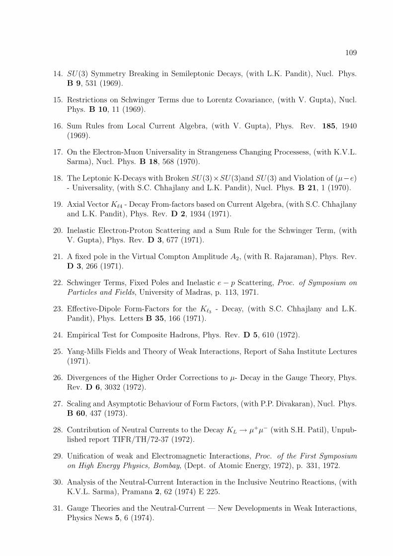
109

14. SU(3) Symmetry Breaking in Semileptonic Decays, (with L.K. Pandit), Nucl. Phys.B 9, 531 (1969).

15. Restrictions on Schwinger Terms due to Lorentz Covariance, (with V. Gupta), Nucl.Phys. B 10, 11 (1969).

16. Sum Rules from Local Current Algebra, (with V. Gupta), Phys. Rev. 185, 1940(1969).

17. On the Electron-Muon Universality in Strangeness Changing Processess, (with K.V.L.Sarma), Nucl. Phys. B 18, 568 (1970).

18. The Leptonic K-Decays with Broken SU(3)×SU(3)and SU(3) and Violation of (µ−e)- Universality, (with S.C. Chhajlany and L.K. Pandit), Nucl. Phys. B 21, 1 (1970).

19. Axial Vector K`4 - Decay From-factors based on Current Algebra, (with S.C. Chhajlanyand L.K. Pandit), Phys. Rev. D 2, 1934 (1971).

20. Inelastic Electron-Proton Scattering and a Sum Rule for the Schwinger Term, (withV. Gupta), Phys. Rev. D 3, 677 (1971).

21. A fixed pole in the Virtual Compton Amplitude A2, (with R. Rajaraman), Phys. Rev.D 3, 266 (1971).

22. Schwinger Terms, Fixed Poles and Inelastic e − p Scattering, Proc. of Symposium onParticles and Fields, University of Madras, p. 113, 1971.

23. Effective-Dipole Form-Factors for the K`3 - Decay, (with S.C. Chhajlany and L.K.Pandit), Phys. Letters B 35, 166 (1971).

24. Empirical Test for Composite Hadrons, Phys. Rev. D 5, 610 (1972).

25. Yang-Mills Fields and Theory of Weak Interactions, Report of Saha Institute Lectures(1971).

26. Divergences of the Higher Order Corrections to µ- Decay in the Gauge Theory, Phys.Rev. D 6, 3032 (1972).

27. Scaling and Asymptotic Behaviour of Form Factors, (with P.P. Divakaran), Nucl. Phys.B 60, 437 (1973).

28. Contribution of Neutral Currents to the Decay KL → µ+µ− (with S.H. Patil), Unpub-lished report TIFR/TH/72-37 (1972).

29. Unification of weak and Electromagnetic Interactions, Proc. of the First Symposiumon High Energy Physics, Bombay, (Dept. of Atomic Energy, 1972), p. 331, 1972.

30. Analysis of the Neutral-Current Interaction in the Inclusive Neutrino Reactions, (withK.V.L. Sarma), Pramana 2, 62 (1974) E 225.

31. Gauge Theories and the Neutral-Current — New Developments in Weak Interactions,Physics News 5, 6 (1974).

110 CHAPTER 16. RAJAJI’S RESEARCH INTERESTS AND PUBLICATIONS

32. Model-Independent Analysis of the Neutral-current Interaction in the Inclusive Neu-trino Reactions, (with K.V.L. Sarma), Pramana 3, 44 (1974).

33. Bounds on the Coupling Constants of the Neutral Current, (with K.V.L. Sarma),Physics Letters B 55, 201 (1975).

34. Theoretical Implications of the Resonance Anomalies in e+e− System, (with S. Pakvasaand S.F. Tuan), Phys. Rev. D 11, 1345 (1975).

35. General Space-Time Structure of the Neutral-Current Interactions, (with S. Pakvasa),Phys. Rev. D 12, 113 (1975).

36. Comments on “Is Bound Charm Found”? (with J. Pasupathy), Phys. Rev. Lett. 34,1250 (1975).

37. Effect of Gluons on Neutral-Current Interactions, (with Probir Roy), Pramana 4, 222(1975).

38. Interpretation of the new particle of the cosmic ray neutrino experiment, (with K.V.L.Sarma), Pramana 5, 78 (1975).

39. Charmed Particles and Anomalies in Antineutrino Collisions, (with K.V.L. Sarma),unpublished report.

40. Colour gluons and scaling in a Unified Gauge Model, (with Probir Roy), Pramana 5,303 (1975).

41. Radiative Decays, Photoproduction and Total Cross Section of ψ - particles, (withK.V.L. Sarma and J. Pasupathy), Pramana 6, 29 (1976).

42. Colour Gluon Excitation at Fermilab, (with Probir Roy), Phys. Rev. Lett. 36 355,689 E (1976).

43. Integral versus Fractional Charges of Quarks - A view through Gauge Theory, Fewbody Dynamics, Edited by A.N. Mitra et al., North Holland p. 341, 1976.

44. General Bounds on the Isovector coupling constants of the weak neutral current, (withK.V.L. Sarma), Pramana 7, 194 (1976).

45. Field Theory of Extended objects (Invited talk), Proc. of the Third Symposium onHigh Energy Physics, Bhubaneswar (Dept. of Atomic Energy, 1976), Vol.II p. 163,1976.

46. Renormalizable Fermi Theory of Weak Interactions (Invited Talk), Proc. of the Inter-national symposium on Frontiers of Theoretical Physics (University of Delhi, 1977), p.121, 1977.

47. Renormalizable Theories from Nonrenormalizable Interactions (with V. Srinivasan),Pramana 9, 239 (1977).

48. Generation of Gluons from Quark Confinement (with V. Srinivasan), Pramana, 10, 33(1973).

111

49. Solitons, Monopoles and Bags (Invited talk), Proc. of the Nuclear Physics and SolidState Physics Symposium, Poona (Dept. of Atomic Energy, 1977) p. 1, 1977.

50. Gauge Theory, Proc. of the Anniversary Symposium of Matscience, Madras (1978).

51. Recent Developments in Gauge Theory, Advances in High Energy Physics (Tata Insti-tute of Fundamental Research, Bombay), Vol. 3, 333 (1977).

52. Neutral Current Cross sections for Neutrinos on Protons (with K.V.L. Sarma) - Pra-mana 11, 609 (1978).

53. Classical Solutions to Quark Confinement (with V. Srinivasan), Pramana 11, 739(1978).

54. The possibility of two-gluon jets in electron-positron annihilation (with S.D. Rindani),Phys. Lett. B 83, 107 (1979).

55. Neutral Currents in left-right symmetric gauge models, (with J.K. Bajaj), Pramana12, 397 (1979).

56. General relations among observables in neutral-current phenomena mediated by oneor two Z bosons, (with M.K. Parida), Pramana 13, 183 (1979).

57. Linking weak interactions with electrodynamics (Popular article) Science Today, p. 17,January 1979.

58. The electroweak mixing angle in unified gauge theories (with J.K. Bajaj) Pramana 14,395 (1980).

59. The electroweak mixing angle in unified gauge theories - the renormalization effects(with J.K. Bajaj), Pramana 14, 411 (1980).

60. Constraints on the parameters of the Left-Right symmetric gauge models (with J.K.Bajaj) Phys. Lett. B 93, 461 (1980).

61. Electron-positron annihilation into three jets in the integer-charge quark model (withS.D. Rindani), Phys. Lett. B 94, 76 (1980).

62. Gauge Theories - A Review, Proc. of the Einstein Centenary Symposium, Ahmedabad,p. 208, 1979.

63. Spin-dependance of the charged gluon contribution in deep inelastic scattering (withH.S. Mani and S.D. Rindani), Physics Lett. B 95, 107 (1980).

64. Contribution of coloured Higgs bosons to e+e− annihilation into two jets (with S.D.Rindani), Physics Lett. B 99, 361 (1981).

65. Contribution of gluons and coloured Higgs bosons to e+e− annihilation into three jets(with S.Lakshmi Bala and S.D. Rindani), Phys. Lett. B 105, 477 (1981).

66. Integer-charged quark model and electorn-positron annihilation into three jets (withS.D. Rindani), Prof. Theor. Phys. 67, 1505 (1982).

112 CHAPTER 16. RAJAJI’S RESEARCH INTERESTS AND PUBLICATIONS

67. Contributions of neutral current couplings in arbitrary two-Z boson extensions of theWeinberg-Salam Model (with J.K. Bajaj) Unpublished report.

68. BAN in unorthodox models - Invited talk in the Proc. of the International Colloquiumon Baryon Nonconservation held at Bombay, p. 65, January 1982.

69. Large-N gauge theory of loops and strings I and II (with H. Bohr) Phys. Rev. D 32,1547, 1553 (1985).

70. Do the PETRA two-photon jet experiments rule out integrally charged quarks? (withT. Jayaraman and S.D. Rindani), Phys. Lett. B 119, 215 (1982).

71. A note on the annihilation of polarised e+e− beams into jets in the broken colour gaugetheory (with S. Lakshmi Bala and S.D. Rindani), Phys. Lett. B 117, 345 (1982).

72. Nonrenormalization of the weak vertex in gauge theories with integrally charged quarks(with M.S. Sriram), Pramana 19 315 (1982).

73. The mass of the electron neutrino and electron capture in 163Ho (with S. Yasumi etal.), Phys. Lett. B 122, 461 (1983).

74. Validity of the equivalent-photon approximation for the production of massive spin-lparticles (with T. Jayaraman and S.D. Rindani), Pramana 26, 21 (1986).

75. Is colour broken by a monopole? (with R. Ramachandran), preprint IIT (Kanpur)report Print-83-0547, 1983, unpublished.

76. Grand Unified Theories - Invited Talk in the Proc. of the VI High Energy PhysicsSymposium, Mysore, (Dept. of Atomic Energy, 1982) p. 1, 1982.

77. Magnetic Monopole - Invited Talk in the Proc. of the Thirty Years Commemorationsymposium, Saha Institute of Nuclear Physics, Calcutta, p. 87, 1983.

78. Decays of W and Z in the broken-colour model (with S. Lakshmibala and S.D. Rindani),Pramana 24, 423 (1985).

79. The recent single-tag two-photon experiments at PETRA and the issue of quark charges(with R.M. Godbole, J.C. Pati, S.D. Rindani and T. Jayaraman), Phys. Lett. B 142,91 (1984).

80. Fields with vanishing colour-currents (with V. Srinivasan and M.S. Sriram), Pramana24, 435 (1985).

81. Modification of the equivalent-photon approximation for the production of massivespin-1 particles (with T. Jayaraman and S.D. Rindani), (unpublished report).

82. Direct Photon Production in e+e− collisions (with T. Jayaraman and S.D. Rindani) -Phys. Rev. D 32, 1262 (1986).

83. Two-photon production in pp and pp collisions (with T. Jayaraman and S.D. Rindani)- Phys. Rev. D 33, 672 (1986).

113

84. What is the next step after electroweak unification? in Recent Advances in TheoreticalPhysics, (World Scientific) Ed: R. Ramachandran, pp. 89-144, 1985.

85. Quantum Interference Effects in a five-dimensional Kaluza-Klein Theory (with R.Parthasarathy and R. Vasudevan), Classical and Quantum Gravity 3, 425 (1986).

86. pp → W−γX as a test of the quark charges (with S. Lakshmibala, X.-G. He and S.Pakvasa), Modern Phys. Lett. A 1, 277 (1986).

87. Higgs Couplings in the integer quark model (with S. Lakshmibala), Pramana 27, 371(1986).

88. e+e− → γ + 2 jets as a test of quark charges (with X.-G. He, S. Pakvasa and S.D.Rindani), Phys. Lett. B 185, 158 (1987).

89. Quantum Interference Effects in a generalized Kaluza - Klein Theory(with R. Parthasarathy and P. Nagarajan), Classical and Quantum Gravity 4 1327(1987).

90. Perspectives in High Energy Physics - Invited talk in the Proc. of the VIII High EnergyPhysics Symposium, Calcutta, p. 399, 1986.

91. Building up the Standard Gauge Model of High Energy Physics, in Gravitation, GaugeTheories and the Early Universe, Ed: B.R. Iyer et al., Kluwer Academic publishers,p.185, 1989.

92. Superstrings - an elementary review, Proc. of the International Conference on Chang-ing Faces of the Physics of Particles & Nuclei, BHU, Varanasi, p. 195, 1987.

93. An Electroweak Factorization Theorem (with S. Lakshmibala) Int. J. Mod. Phys. A4, 2977 (1989).

94. Introduction to String Theories, in Gravitation, Quantum Fields and Superstrings(World Scientific, Singapore), pp. 333-393, 1988.

95. Is Quantum Mechanics Forever? Preprint TIFR/TH/89-13 (to be published in Philo-sophical Foundations of Quantum Theory, World Scientific, Singapore), 1989.

96. Interpretation of the recent Kolar events (with A.S. Joshipura, V. Gupta and K.V.L.Sarma), Pramana 33, 639 (1989).

97. Stability of the S matrix pole (with S.S. Vasan), Pramana 34, 183 (1990).

98. Mass shifts for the weak bosons in the integrally charged quark model (with N.G.Deshpande), Mod. Phys. Lett. A 5, 301 (1990).

99. Electroweak radiative corrections and the masses of the weak bosons, in Phenomenologyof the Standard Model and Beyond (World Scientific, Singapore), p. 407, 1989.

100. Electroweak Symmetry, in Proc. of Raman Centenary Symposium on Waves andSymmetry, Current Science 59, 1080 (1990).

114 CHAPTER 16. RAJAJI’S RESEARCH INTERESTS AND PUBLICATIONS

101. Rosenbluth scattering with Pauli moment for the electron (with R. Basu and M.V.N.Murthy), J. Phys. G 17, 401 (1991).

102. Algebra for fermions with a new exclusion principle (with A.K.Mishra), Pramana 36,537 (1991).

103. The discovery of Dirac equation and its impact on present-day Physics, in Dirac andFeynman : Pioneers in Quantum Mechanics, Ed. by R. Dutt and A.K. Ray, WileyEastern, p. 9 (1993).

104. The future of high energy physics (Keynote address), in Particle Phenomenology inthe 90’s, Ed.: A. Datta et al., World Scientific, p. 1 (1992).

105. Two Topics in Electroweak Physics : Radiative Corrections and Baryon Number Vio-lation, in Particle Phenomenology in the 90’s, Ed. by A. Datta et al., World Scientific,p. 404 (1992).

106. New forms of quantum statistics (with A.K. Mishra) Pramana 38, L 411 (1992).

107. Orthosupersymmetric quantum mechanics (with A. Khare and A.K. Mishra), Int. J.Mod. Phys. A 8 1245 (1993).

108. Parasupersymmetric quantum mechanics and its infinite order (with A. Khare andA.K. Mishra), Mod. Phys. Lett. A 8 107 (1993).

109. Algebras of creation and destruction operators (with A.K. Mishra), Pramana, J. Phys.40 149 (1993).

110. Quantum field theory of orthofermions and orthobosons (with A.K. Mishra), Mod.Phys. Lett. A 7 3425 (1992).

111. Complex q-mutator algebra and fractional statistics (with A.K. Mishra), Mod. Phys.Lett A 9 419 (1994).

112. “Infinite Statistics” and its two-parameter deformation (with A.K. Mishra), Phys.Lett. A 138 210 (1994).

113. An algebra for ordered particles (with A.K.Mishra) – Phys. Lett. A 203, 153 (1995).

114. Is there a future for High Energy Physics? in Proc. of the Int. Conf. on NonAccelerator Particle Physics, Bangalore, p. 4, 1994 Ed: R. Cowsik, World Scientific,1994.

115. Generalized Fock spaces, new forms of quantum statistics and their algebras (withA.K. Mishra) Pramana - J. Phys. 45 91 (1995).

116. A new mechanism for neutrino masses in supersymmetric SO(10) grand unification(with K.S. Babu and M.K. Parida) – preprint IMSc-94/19 (to be published).

117. New forms of quantum statistics and generalized Fock spaces, in Bose and 20th Cen-tury Physics, Kluwer Academic Publishers (The Netherlands), Ed: Partha Ghose andAbhijit Mookerji, 1995.

115

118. Generalized Fock spaces, and new forms of quantum statistics, in Current Trends inMathematics and Physics (A tribute to Harish Chandra) Ed: S.D. Adhikari, NarosaPublishing House, New Delhi, p. 138, 1995.

119. An unified treatment of quantum interference effects (with R. Parthasarathy and R.Vasudevan), in Selected Topics in Mathematical Physics (Prof. R. Vasudevan MemorialVolume), Ed: R. Sridhar et al., Allied Publishers Ltd., Madras, p. 279, 1995.

120. Leptons and quarks as composites of orthofermions, in Selected Topics in Mathemat-ical Physics (Prof. R. Vasudevan Memorial Volume), Ed: R. Sridhar et al., AlliedPublishers Ltd., Madras, p. 288, 1995.

121. Solar and atmospheric neutrino oscillations with three flavours (with Mohan Narayan,M.V.N. Murthy and S. Uma Sankar) Phys. Rev. D 53 2809 (1996).

122. Atmospheric neutrinos with three flavour mixing (with Mohan Narayan and S. UmaSankar) Phys. Rev. D 56 437 (1997).

123. Fock space representation of differential calculus on the noncommutative quantumspace, (with A.K. Mishra) J. Math. Phys. 38 466 (1997).

124. Solar eclipse and neutrinos (with Mohan Narayan and Rahul Sinha), Current Science70 848 (1996), 72 417 (E) (1997).

125. Time-of-night variation of solar neutrinos (with Mohan Narayan and Rahul Sinha),Mod. Phys. Lett. A 13 1915 (1998).

126. Solar neutrinos and the eclipse effect (with Mohan Narayan, Rahul Sinha and C.P.Burgess), Phys. Rev. D 60, 073006 (1999).

127. Dynamics in a noncommutative phase space (with R.P. Malik and A.K. Mishra), Int.Journal of Mod. Phys. A 13, 4759 (1998).

128. Perspectives in High Energy Physics, Indian J. Phys. A 72, 679 (1998).

129. High Energy Physics in the 21st Century - An overview, Current Science 71 109 (1996).

130. Particles and Fields (Status Report) in Physics in India, Indian National ScienceAcademy, New Delhi, p. 41, 1996.

131. Fock space for noncommutative calculus, in Special Functions and Differential Equa-tions Ed: K. Srinivasa Rao et al., Allied Publishers, p. 280, 1998.

132. Three flavour implications of the result of the CHOOZ Collaboration (with MohanNarayan and S. Uma Sankar), Phys. Rev. D 58, 031301 (1998).

133. One pion events by atmospheric neutrinos (with K.R.S. Balaji and S. Uma Sankar),Int. J. Mod. Phys. A 16, 1417 (2001).

134. A new mechanism for neutrino mass (with P.P. Divakaran), Mod. Phys. Lett. A 14,913 (1999).

116 CHAPTER 16. RAJAJI’S RESEARCH INTERESTS AND PUBLICATIONS

135. Neutrinos from stellar collapse : effects of flavour mixing (with G. Dutta, D. Indumathiand M.V.N.Murthy), Phys. Rev. D 61, 13009 (2000).

136. Constraints on the mixing angles of Majorana neutrinos (with R. Adhikari), Phys.Rev. D 61, 031301 (2000).

137. Hierarchical four-neutrino oscillations with a decay option (with E. Ma and I. Stancu),Phys. Rev. D 61, 071302 (R) (2000).

138. A new differential calculus on noncommutative spaces (with R.P. Malik and A.K.Mishra), preprint math-ph/9908001, 1999.

139. Phenomenology of neutrino oscillations, hep-ph/0004154 and Pramana 55, 19 (2000).

140. Three inequivalent Mass-degenerate Majorana neutrinos and a model of their splittingfor neutrino oscillations (with R. Adhikari and E. Ma), Phys. Lett. B486, 134 (2000).

141. Neutrinos from Stellar Collapse: Comparison of the effects of three and four flavourmixings. (with G. Dutta, D. Indumathi and M.V.N. Murthy) Phys. Rev. D 62,093014 (2000).

142. Light sterile neutrinos from large extra dimensions (with E. Ma and Utpal Sarkar),Phys. Lett. B 495, 363 (2000).

143. Neutrinos from Stellar Collapse: Comparison of signatures in water and heavy water de-tectors (with G. Dutta, D. Indumathi and M.V.N. Murthy), preprint hep-ph/0101093,to appear in Phys. Rev. D, 2001.

144. Softly broken A4 symmetry from nearly degenerate neutrino masses (with E. Ma),preprint hep-ph/0106291 (To appear in Phys. Rev. D, 2001).

145. Light unstable sterile neutrino (with E. Ma), preprint hep-ph/0107203 ( to appear inPhys. Rev. D,2001).

146. Anomalous magnetic moment of muon and L-violating Supersymmetric Models (withR. Adhikari), preprint hep-ph/0107279.

147. Supersymmetric model of muon anomalous magnetic moment and neutrino masses(with R. Adhikari and E. Ma), preprint hep-ph/0108167.

148. Double threefold degeneracies for active and sterile neutrinos (with E. Ma), preprinthep-ph/0109236 (to appear in Mod. Phys. Lett. A).

Rajaji Symposium

P R O G R A M M E S C H E D U L E

22 February 2001

Each talk is of 20 minute duration with 5 minutes time for Chairman’sremarks.

09:15 -9:30 R.Ramachandran Inaugural address09:30–10:45 Session 1 T. Pradhan- Chair09:35–09:55 Lalit Sehgal 1968 - 1973: Some Reminiscences10:00–10:20 P.P.Divakaran Composite Fields and Fermion Masses10:25–10:45 C.S.Unnikrishnan Proof of absence of spooky action at a distance in

Quantum Correlations10:45–11:15 T E A B R E A K11:15–13:00 Session 2 P M Mathews - Chair11:20–11:40 S. Krishnagopal Are Accelerators needed for High Energy Physics?11:45–12:05 Avinash Khare Para and Ortho Supersymmetric Quantum Me-

chanics12:10–12:30 A.K.Mishra Fock Spaces and Quantum Statistics12:35–12:55 H.S.Mani Overview of Semi-inclusive DIS Processes13:00–14:00 L U N C H B R E A K14:00–15:40 Session 3 J. Pasupathy - Chair14:05–14:25 Rohini Godbole Physics at future colliders14:30–14:50 R. Cowsik Direct Neutrino Mass Measurements14:55–15:15 R.Parthasarathy Kaluza-Klein Idea: Ups, Downs and Strange15:20–15:40 R.P.Malik Quantum Groups, q-dynamics and Rajaji15:45–16:10 T E A B R E A K16:10–17:30 Session 4 R. K. Kaul - Chair16:15–16:35 T.Jayaraman Solitons in String Theory Compactifications16:40–17:00 V.Srinivasan Ramblings17:05–17:25 M.S.Sriram Geometric Description of Hamiltonian Chaos18:30–20:00 Evening Session R. Balasubramanian - Chair

Open Session20:00 Symposium Dinner hosted by the Director