3 testing spatial randomness - penn engineeringese502/notebook/part_i/3_testing_spatial... · but...

NOTEBOOK FOR SPATIAL DATA ANALYSIS Part I. Spatial Point Pattern Analysis ______________________________________________________________________________________

________________________________________________________________________ ESE 502 I.3-1 Tony E. Smith

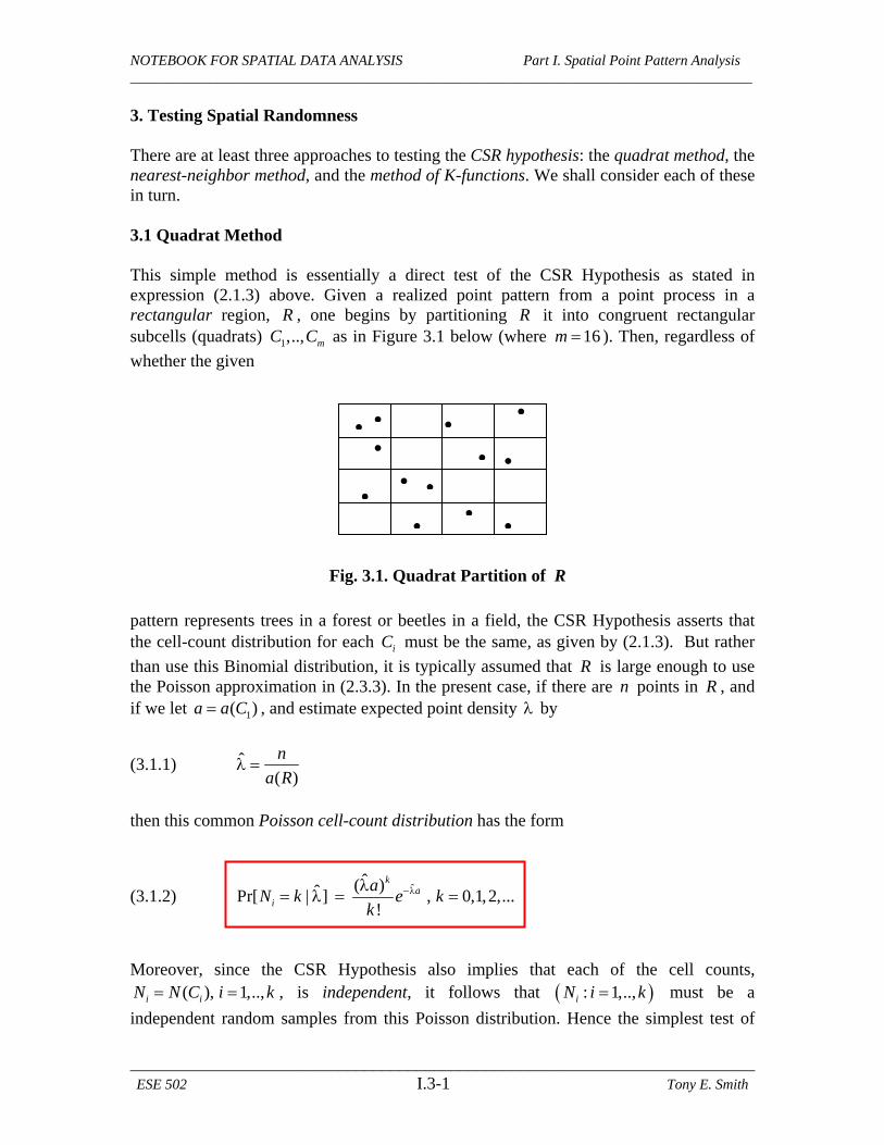
3. Testing Spatial Randomness There are at least three approaches to testing the CSR hypothesis: the quadrat method, the nearest-neighbor method, and the method of K-functions. We shall consider each of these in turn. 3.1 Quadrat Method This simple method is essentially a direct test of the CSR Hypothesis as stated in expression (2.1.3) above. Given a realized point pattern from a point process in a rectangular region, R , one begins by partitioning R it into congruent rectangular subcells (quadrats) 1,.., mC C as in Figure 3.1 below (where 16m ). Then, regardless of

whether the given pattern represents trees in a forest or beetles in a field, the CSR Hypothesis asserts that the cell-count distribution for each iC must be the same, as given by (2.1.3). But rather

than use this Binomial distribution, it is typically assumed that R is large enough to use the Poisson approximation in (2.3.3). In the present case, if there are n points in R , and if we let 1( )a a C , and estimate expected point density by

(3.1.1) ˆ( )

n

a R

then this common Poisson cell-count distribution has the form

(3.1.2) ˆˆ( )ˆPr[ | ] , 0,1,2,...

!

ka

i

aN k e k

k

Moreover, since the CSR Hypothesis also implies that each of the cell counts,

( ), 1,..,i iN N C i k , is independent, it follows that : 1,..,iN i k must be a

independent random samples from this Poisson distribution. Hence the simplest test of

Fig. 3.1. Quadrat Partition of R


________________________________________________________________________ ESE 502 I.3-2 Tony E. Smith

this hypothesis is to use the Pearson 2 goodness-of-fit test. Here the expected number of points in each cell is given by the mean of the Poisson above, which (recalling that

( ) /a a R m by construction) is

(3.1.3) ˆ ˆ( | )( )

n nE N a a

a R m

Hence if the observed value of iN is denoted by in , then the chi-square statistic

(3.1.4) 2

2

1

( / )

/

m ii

n n m

n m

is known to be asymptotically chi-square distributed with 1m degrees of freedom, under the CSR Hypothesis. Thus one can test this hypothesis directly in these terms. But

since /n m is simply the sample mean, i.e., 1

/ (1/ )m

iin m m n n

, this statistic can also

be written as

(3.1.5) 2 2

2

1

( )( 1)

m ii

n n sm

n n

where 2 2

11

1 ( )m

iims n n is the sample variance. But since the variance if the Poisson

distribution is exactly the mean, it follows that var( ) / ( ) 1N E N under CSR. Moreover,

since 2 /s n is the natural estimate of this ratio, this ratio is often designated as the index of dispersion, and used as a rough measure of dispersion versus clustering. If 2 / 1s n then there is too little variation among quadrat counts, suggesting possible “dispersion” rather than randomness. Similarly, if 2 / 1s n then there is too much variation among counts, suggesting possible “clustering” rather than randomness. But this testing procedure is very restrictive in that it requires an equal-area partition of the given region.1 More importantly, it depends critically on the size of the partition chosen. As with all applications of Pearson’s goodness-of-fit test, if there is no natural choice of partition size, then the results can be very sensitive to the partition chosen. 3.2 Nearest-Neighbor Methods In view of these shortcomings, the quadrat method above has for the most part been replaced by other methods. The simplest of these is based on the observation that if one simply looks at distances between points and their nearest neighbors in R , then this provides a natural test statistic that requires no artificial partitioning scheme. More

1 More general “random quadrat” methods are discussed in Cressie (1995,section 8.2.3).


________________________________________________________________________ ESE 502 I.3-3 Tony E. Smith

precisely, for any given points, 1 2( , )s s s and 1 2( , )v v v in R we denote the

(Euclidean) distance between s and v by2

(3.2.1) 2 21 1 2 2( , ) ( ) ( )d s v s v s v

and denote each point pattern of size n in R by ( : 1,.., )n iS s i n , then for any point,

i ns S ,3 the nearest neighbor distance (nn-distance) from is to all other points in nS is

given by4 (3.2.2) ( ) min{ ( , ) : , }i i n i j j nd d S d s s s S j i

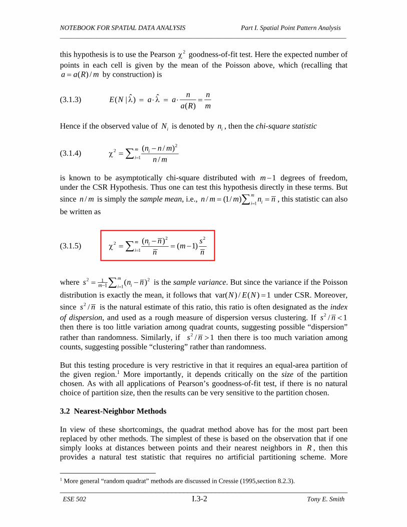
In a manner similar to the index of dispersion above, the average magnitudes of these nn-distances (relative to those expected under CSR) provide a direct measure of “dispersion” or “clustering” in point patterns. This is seen clearly by comparing of the two figures below, each showing a pattern of 14 points. In Figure 3.2 these points are seen to be very uniformly spaced, so that nn-distances tend to be larger than what one would expect under CSR. In Figure 3.3 on the other hand, the points are quite clustered, so that nn-distances tend to be smaller than under CSR.

2 Throughout these notes we shall always take ( , )d s v to be Euclidean distance. However there are many

other possibilities. At large scales it may be more appropriate to use great-circle distance on the globe. Alternatively, one may take ( , )d s v to be travel distance on some underlying transportation network. In

any case, most of the basic concepts developed here (such as nearest neighbor distances) are equally meaningful for these definitions of distance. 3 The vector notation, ( : 1,.., )

n iS s i n , means that each point

is is treated as a distinct component of

nS . Hence (with a slight abuse of notation), we take

i ns S to mean that

is is a component of pattern

nS .

4 This is called the event-event distance in [BG] (p.98). One may also consider the nn-distance from any

random point, x R to the given pattern as defined by ( min{ ( , ) : 1, .., })ix nd S d x s i n . However, we

shall not make use of these point-event distances here. For a more detailed discussion see Cressie (1995, section 8.2.6).

Fig.3.2. Dispersed Pattern Fig.3.3. Clustered Pattern


________________________________________________________________________ ESE 502 I.3-4 Tony E. Smith

3.2.1 Nearest-Neighbor Distribution under CSR To make these ideas precise, we must determine the probability distribution of nn-distance under CSR, and compare the observed nn-distance with this distribution. To begin with, suppose that the implicit reference region R is large, so that for any given point density, , we may assume that cell-counts are Poisson distributed under CSR. Now suppose that s is any randomly selected point in a pattern realization of this CSR process, and let the random variable, D , denote the nn-distance from s to the rest of the pattern. To determine the distribution of D , we next consider a circular region, dC , of

radius d around s , as shown in Figure 3.4 below. Then by definition, the probability that D is at least equal to d is precisely the probability that there are no other points in dC . Hence if

we now let ( ) { }d dC s C s , then this proba-

bility is given by (3.2.3) Pr( ) Pr{ [ ( )] 0}dD d N C s

But since the right hand side is simply a cell-count probability, it follows from expression (2.3.3) that,

(3.2.4) 2[ ( )]Pr( ) da C s dD d e e

where the last equality follows from the fact that 2[ ( )] ( )d da C s a C d . Hence it

follows by definition that the cumulative distribution function (cdf), ( )DF d , for D is

given by,

(3.2.5) 2

( ) Pr( ) 1 Pr( ) 1 dDF d D d D d e

In Section 2 of the Appendix to Part I it is shown that this is an instance of the Rayleigh distribution, and in Section 3 of the Appendix that for a random sample of m nearest-neighbor distances 1( ,.., )mD D from this distribution, the scaled sum (known as Skellam’s

statistic),

(3.2.6) 2

12

m

m iiD

S

is chi-square distributed with 2m degrees of freedom (as on p.99 in [BG]). Hence this statistic provides a test of the CSR Hypothesis based on nearest neighbors.

sd

dC

R

Fig.3.4. Cell of radius d


________________________________________________________________________ ESE 502 I.3-5 Tony E. Smith

3.2.2 Clark-Evans Test While Skellam’s statistic can be used to construct tests, it follows from the Central Limit Theorem that independent sums of identically distributed random variables are approximately normally distributed.5 Hence the most common test of the CSR Hypothesis based on nearest neighbors involves a normal approximation to the sample mean of D , as defined by

(3.2.7) 1

1 m

m iimD D

To construct this normal approximation, it is shown in Section 2 of the Appendix to Part I that mean and variance of the distribution in (3.2.4) are given respectively by

(3.2.8) 1

( )2

E D

(3.2.9) 4

var( )4

D

To get some feeling for these quantities observe that under the CSR Hypothesis, as the point density, , increases, both the expected value and variance of nn-distances decrease. This makes intuitive sense when one considers denser scatterings of random points in R .

Next we observe from the properties of independently and identically distributed ( iid ) random samples that for the sample mean, mD , in (3.2.7) we must then have

(3.2.10) 1 111 1 1

( ) ( ) [ ( )] ( )2

m

m iim mE D E D mE D E D

and similarly must have

(3.2.11) 2

2

111 1 4

var( ) var( ) [ var( )](4 )

m

m iim mD D m Dm

But from the Central Limit Theorem it then follows that for sufficiently large sample sizes,6 mD must be approximately normally distributed under the CSR Hypothesis with

mean and variance given by (3.2.10) and (3.2.11), i.e., that:

(3.2.12) 1 4

~ ,(4 )2

mD Nm

5 See Section 3.1.4 in Part II of this NOTEBOOK for further detail. Here we simply state those results needed for the Clark-Evans test. 6 Here “sufficiently large” is usually taken to mean 30m , as long as the distribution in (3.2.4) is not “too skewed”. Later we shall investigate this by using simulations.


________________________________________________________________________ ESE 502 I.3-6 Tony E. Smith

Hence this distribution provides a new test of the CSR Hypothesis, known as the Clark-Evans Test [see Clark and Evans (1954) and [BG], p.100]. If the standard error of mD is

denoted by

(3.2.13) var( ) (4 ) 4m mD D m

then to construct this test, one begins by standardizing the sample mean, mD , in order to

use the standard normal tables. Hence, if we now denote the standardized sample mean under the CSR Hypothesis by

(3.2.14)

( ) [1/(2 )]

( ) (4 ) 4m m m

mm

D E D DZ

D m

then it follows at once from (3.2.12) that under CSR,7 (3.2.15) ~ (0,1)mZ N

To construct a test of the CSR Hypothesis based on this distribution, suppose that one starts with a sample pattern ( : 1,.., )n iS s i n and constructs the nn-distance id for each

point, i ns S . Then it would seem most natural to use all these distances 1( ,.., )nd d to

construct the sample-mean statistic in (3.2.10) above. However, this would violate the assumed independence of nn-distances on which this distribution theory is based. To see this it is enough to observe that if is and js are mutual nearest neighbors, so that i jd d ,

then these are obviously not independent. More generally, if js is the nearest neighbor of

is , then again id and jd must be dependent.8

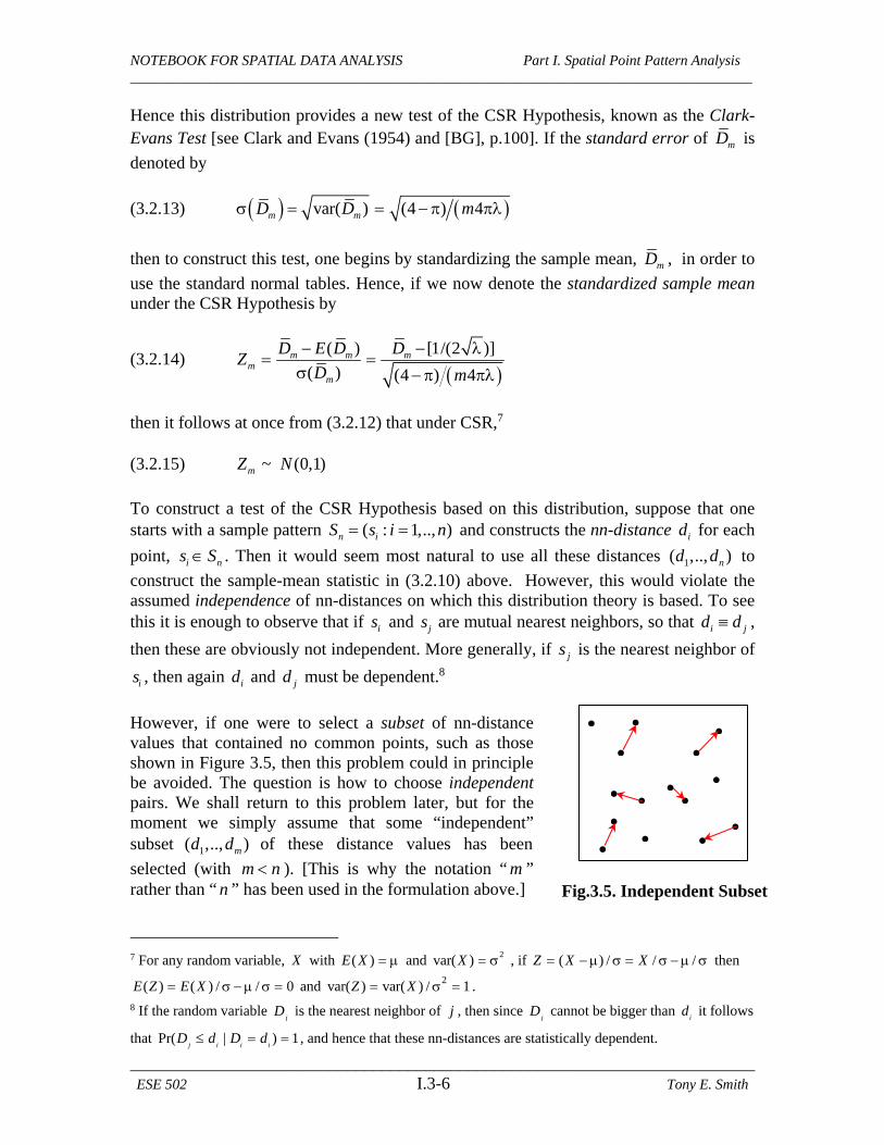
However, if one were to select a subset of nn-distance values that contained no common points, such as those shown in Figure 3.5, then this problem could in principle be avoided. The question is how to choose independent pairs. We shall return to this problem later, but for the moment we simply assume that some “independent” subset 1( ,.., )md d of these distance values has been

selected (with m n ). [This is why the notation “ m ” rather than “ n ” has been used in the formulation above.]

7 For any random variable, X with ( )E X and 2var( )X , if ( ) / / /Z X X then

( ) ( ) / / 0E Z E X and 2var( ) var( ) / 1Z X . 8 If the random variable

jD is the nearest neighbor of j , then since

jD cannot be bigger than

id it follows

that Pr( | ) 1j i i i

D d D d , and hence that these nn-distances are statistically dependent.

Fig.3.5. Independent Subset


________________________________________________________________________ ESE 502 I.3-7 Tony E. Smith

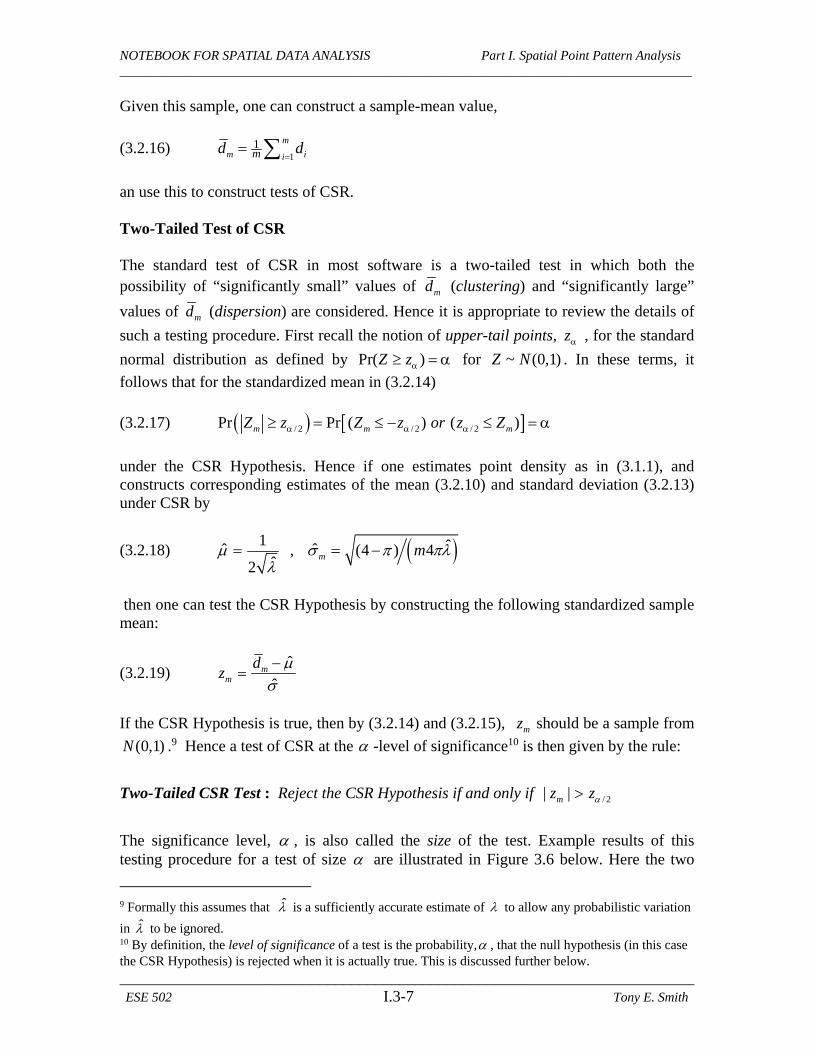
Given this sample, one can construct a sample-mean value,

(3.2.16) 1

1 m

m iimd d

an use this to construct tests of CSR. Two-Tailed Test of CSR The standard test of CSR in most software is a two-tailed test in which both the possibility of “significantly small” values of md (clustering) and “significantly large”

values of md (dispersion) are considered. Hence it is appropriate to review the details of

such a testing procedure. First recall the notion of upper-tail points, z , for the standard

normal distribution as defined by Pr( )Z z for ~ (0,1)Z N . In these terms, it

follows that for the standardized mean in (3.2.14)

(3.2.17) / 2 / 2 / 2Pr Pr ( ) ( )m m mZ z Z z or z Z

under the CSR Hypothesis. Hence if one estimates point density as in (3.1.1), and constructs corresponding estimates of the mean (3.2.10) and standard deviation (3.2.13) under CSR by

(3.2.18) 1

ˆˆ2

, ˆˆ (4 ) 4m m

then one can test the CSR Hypothesis by constructing the following standardized sample mean:

(3.2.19) ˆ

ˆm

m

dz

If the CSR Hypothesis is true, then by (3.2.14) and (3.2.15), mz should be a sample from

(0,1)N .9 Hence a test of CSR at the -level of significance10 is then given by the rule:

Two-Tailed CSR Test : Reject the CSR Hypothesis if and only if / 2| |mz z

The significance level, , is also called the size of the test. Example results of this testing procedure for a test of size are illustrated in Figure 3.6 below. Here the two

9 Formally this assumes that ̂ is a sufficiently accurate estimate of to allow any probabilistic variation

in ̂ to be ignored. 10 By definition, the level of significance of a test is the probability, , that the null hypothesis (in this case the CSR Hypothesis) is rejected when it is actually true. This is discussed further below.


________________________________________________________________________ ESE 502 I.3-8 Tony E. Smith

samples, mz , in the tails of the distribution are seen to yield strong evidence against the

CSR Hypothesis, while the sample in between does not. One-Tailed Tests of Clustering and Dispersion As already noted, values of md (and hence mz ) that are too low to be plausible under

CSR are indicative of patterns more clustered than random. Similarly, values too large are indicative of patterns more dispersed than random. In many cases, one of these alternatives is more relevant than the other. In the redwood seedling example of Figure 1.1 it is clear that trees appear to be clustered. Hence the only question is whether or not

Fig.3.6. Two-Tailed Test of CSR this apparent clustering could simply have happened by chance. So the key question here is whether this pattern is significantly more clustered than random. Similarly, one can ask whether the pattern of Cell Centers in Figure 1.2 is significantly more dispersed than random. Such questions lead naturally to one-tailed versions of the test above. First, a test of clustering versus the CSR Hypothesis at the -level of significance is given by the rule: Clustering versus CSR Test : Conclude significant clustering if and only if mz z

Example results of this testing procedure for a test of size are illustrated in Figure 3.7 below. Here the standardized sample mean mz to the right is sufficiently low to conclude

the presence of clustering (at the -level of significance), and the sample toward the middle is not.

/ 2 / 2

0 mz

Reject CSR

mz

Reject CSR

mz

Do Not Reject

/ 2z / 2z


________________________________________________________________________ ESE 502 I.3-9 Tony E. Smith

Fig.3.7. One-Tailed Test of Clustering In a similar manner, one can construct a test of dispersion versus the CSR Hypothesis at the -level of significance using the rule: Dispersion versus CSR Test : Conclude significant dispersion if and only if mz z

Example results for a test of size are illustrated in Figure 3.8 below, where the sample

mz to the left is sufficiently high to conclude the presence of dispersion (at the -level of

significance) and the sample toward the middle is not.

Fig.3.8. One-Tailed Test of Dispersion While such tests are standard in literature, it is important to emphasize that there is no “best” choice of . The typical values given by most statistical texts are listed in Tables 3.1 and 3.2 below: Table 3.1. Two-Tailed Significance Table3.2. One-Tailed Significance

z 0

mz

No Significant Dispersion

mz

Significant Dispersion

Significance / 2z“Strong” .01 2.58“Standard” .05 1.96“Weak” .10 1.65

Significance z

“Strong” .01 2.33 “Standard” .05 1.65 “Weak” .10 1.28

z 0

mz mz

Significant Clustering

No Significant Clustering


________________________________________________________________________ ESE 502 I.3-10 Tony E. Smith

So in the case of a two-tailed test, for example, the non-randomness of a given pattern is considered “strongly” (“weakly”) significant if the CSR Hypothesis can be rejected at the

.01 ( .10) level of significance.11 The same is true of one-tailed tests (where the

cutoff value, / 2z , is now replaced by z ). In all cases, the value .05 is regarded as a

standard (default) value indicating “significance”. P-Values for Tests However, since these distinctions are admittedly arbitrary, another approach is often adopted in evaluating test results. The main idea is quite intuitive. In the one-tailed test of clustering versus CSR above, suppose that for the observed standardized mean value, mz ,

one simply asks how likely it would be to obtain a value this low if the CSR Hypothesis were true? This question is easily answered by simply calculating the probability of a sample value as low as mz for the standard normal distribution (0,1)N . If the cumulative

distribution function for the normal distribution is denoted by (3.2.20) ( ) Pr( )z Z z then this probability, called the P-value of the test, is given by (3.2.21) Pr( ) ( )m mZ z z

as shown graphically below:

Fig.3.9. P-value for Clustering Test Notice that unlike the significance level, , above, the P-value for a test depends on the realized sample value, mz , and hence is itself a random variable that changes from

sample to sample. However, it can be related to by observing that if ( )mP Z z ,

then for a test of size , one would conclude that there is significant clustering. More generally the P-value, ( )mP Z z can be defined as the largest level of significance

(smallest value of ) at which CSR would be rejected in favor of clustering based on the given sample value, mz .

Similarly, one can define the P-value for a test of dispersion the same way, except that now for a given observed standardized mean value, mz , one asks how likely it would be to

11 Note that lower values of denote higher levels of significance.

0 mz

( )mz


________________________________________________________________________ ESE 502 I.3-11 Tony E. Smith

obtain a value this large if the CSR Hypothesis were true. Hence the P-value in this case is given simply by (3.2.22) Pr( ) Pr( ) 1 Pr( ) 1 ( )m m m mZ z Z z Z z z

where the first equality follows from the fact that Pr( ) 0mZ z for continuous

distributions.12 This P-value is illustrated graphically below:

Fig.3.10. P-Value for Dispersion Test Finally, the corresponding P-value for the general two-tailed test is given as the answer to the following question: How likely would it be to obtain a value as far from zero as mz if

the CSR Hypothesis were true? More formally this P-value is given by (3.2.23) (| | ) 2 ( | |)m mP Z z z

as shown below. Here the absolute value is used to ensure that | |mz is negative

regardless of the sign of mz . Also the factor “2” reflects the fact that values in both tails

are further from zero than mz .

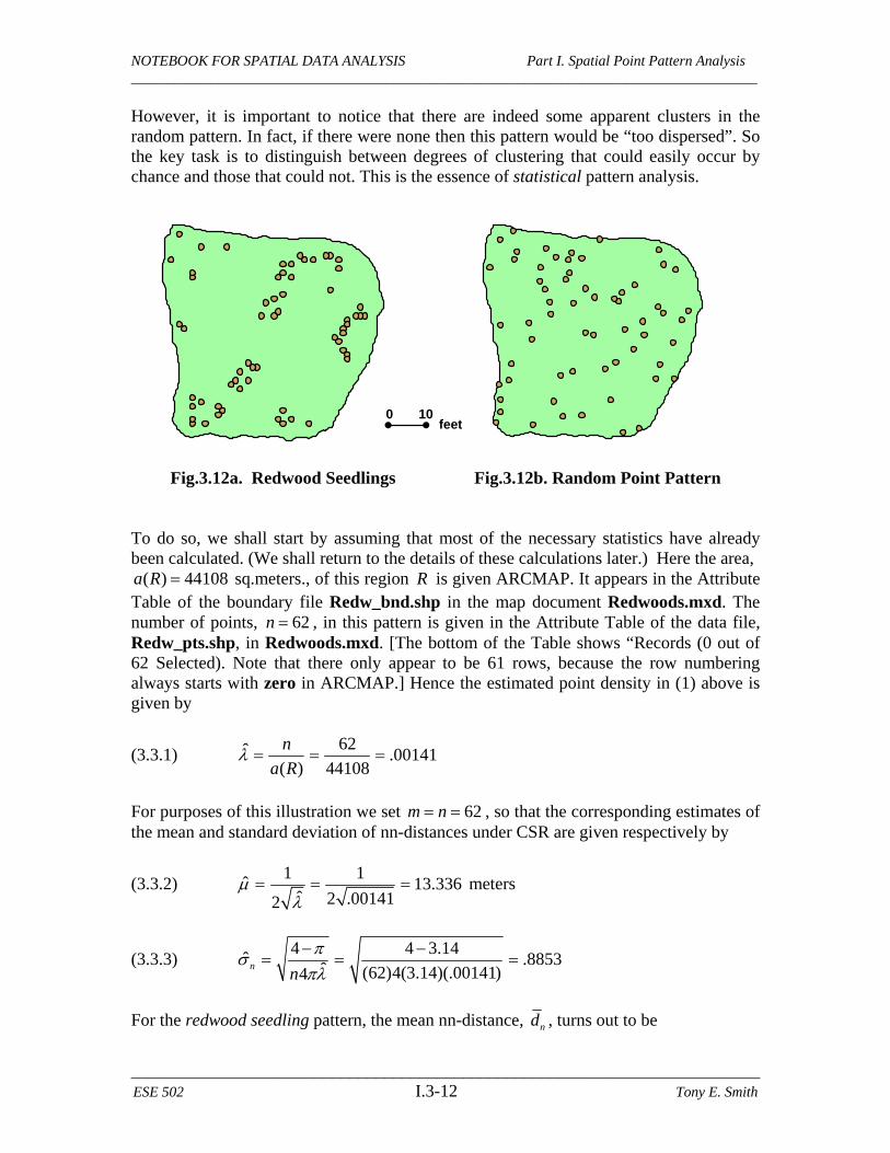
Fig.3.11. P-Value for Two-Tailed Test 3.3 Redwood Seedling Example We now illustrate the Clark-Evans testing procedure in terms of the Redwood Seedling example in Figure 1.1. This image is repeated in Figure 3.12a below, where it is compared with a randomly generated point pattern of the same size in Figure 3.12b. Here it is evident that the redwood seedlings are more clustered than the random point pattern. 12 By the symmetry of the normal distribution, this P-value is also given by ( ) [ 1 ( )]

m mz z .

0

1 ( )mz

mz

0

| |mz

( | |)mz ( | |)mz


________________________________________________________________________ ESE 502 I.3-12 Tony E. Smith

However, it is important to notice that there are indeed some apparent clusters in the random pattern. In fact, if there were none then this pattern would be “too dispersed”. So the key task is to distinguish between degrees of clustering that could easily occur by chance and those that could not. This is the essence of statistical pattern analysis. Fig.3.12a. Redwood Seedlings Fig.3.12b. Random Point Pattern To do so, we shall start by assuming that most of the necessary statistics have already been calculated. (We shall return to the details of these calculations later.) Here the area,

( ) 44108a R sq.meters., of this region R is given ARCMAP. It appears in the Attribute Table of the boundary file Redw_bnd.shp in the map document Redwoods.mxd. The number of points, 62n , in this pattern is given in the Attribute Table of the data file, Redw_pts.shp, in Redwoods.mxd. [The bottom of the Table shows “Records (0 out of 62 Selected). Note that there only appear to be 61 rows, because the row numbering always starts with zero in ARCMAP.] Hence the estimated point density in (1) above is given by

(3.3.1) 62ˆ .00141

( ) 44108

n

a R

For purposes of this illustration we set 62m n , so that the corresponding estimates of the mean and standard deviation of nn-distances under CSR are given respectively by

(3.3.2) 1 1

ˆ 13.336ˆ 2 .001412

meters

(3.3.3) 4 4 3.14

ˆ .8853ˆ (62)4(3.14)(.00141)4

nn

For the redwood seedling pattern, the mean nn-distance, nd , turns out to be

10 0

feet


________________________________________________________________________ ESE 502 I.3-13 Tony E. Smith

(3.3.4) 9.037nd meters

At this point, notice already that this average distance is much smaller than the theoretical value calculated in (3.3.2) under the hypothesis of CSR. So this already suggests that for the given density of trees in this area, individual trees are much too close to their nearest neighbors to be random. To verify this statistically, let us compute the standardized mean

(3.3.5) ˆ 9.037 13.336

4.855ˆ .8853

nn

n

dz

Now recalling from Table 2 above that there is “strongly significant” clustering if

.01 2.33nz z , one can see from (3.3.5) that clustering in the present case is even

more significant. In fact the P-value in this case is given by13

(3.3.6) P-value ( ) ( ) ( 4.855) .0000006n nP Z z z

(Methods for obtaining -values are discussed below). So the chances of obtaining a mean nearest-neighbor distance this low under the CSR hypothesis are less than one in a million. This is very strong evidence in favor of clustering versus CSR. However, one major difficulty with this conclusion is that we have used the entire point pattern ( )m n , and have thus ignored the obviously dependencies between nn-distances discussed above. Cressie (1993, p.609-10) calls this “intensive” sampling, and shows with simulation analyses that this procedure tends to overestimate the significance of clustering (or dispersion). The basic reason for this is that positive correlation among nn-distances results in a larger variance of the test statistic, nZ , than would be expected

under independence (for a proof of this see Section 4 of the Appendix to Part I, and also see p.99 in [BG]). Failure to account for this will tend to inflate the absolute value of the standardized mean, thus exaggerating the significance of clustering (or dispersion). With this in mind, we now consider two procedures for taking random subsamples of pattern points that tend to minimize this dependence problem. These two approaches utilize JMPIN and MATLAB, respectively, and thus provide convenient introductions to using these two software packages.

3.3.1 Analysis of Redwood Seedlings using JMPIN One should begin here by reading the notes on opening JMPIN in section 2.1 of Part IV in this NOTEBOOK.14 In the class subdirectory jmpin now open the file, Redwood_data.jmp in JMPIN. (The columns nn-dist and area contain data exported from MATLAB and ARCMAP, respectively, and are discussed later). The column Rand_Relabel is a random ordering of labels with associated nn-distance values in the

13 Methods for obtaining -values are discussed later. 14 This refers to section 2.1 in the Software portion (Part IV) of this NOTEBOOK. All other references to software procedures will be done similarly.


________________________________________________________________________ ESE 502 I.3-14 Tony E. Smith

column, Sample. [These can be constructed using the procedure outlined in section 2.2(2) of Part IV in this NOTEBOOK.] Now open a second file, labeled CE_Tests.jmp, which is a spreadsheet constructed for this class that automates Clark-Evans tests. Here we shall use a random 50% subsample of points from the Redwood Seedlings data set to carry out a test of clustering.15 To do

so, click Rows Add Rows and add 31 rows ( 62 / 2) . Next, copy-and-paste the first

31 rows of Redwood_data.jmp into these positions. In Redwood_data.jmp : (i) Select rows 1 to 31 (click Row 1, hold down shift, and click Row 31) (ii) Select column heading Sample (this entire column is now selected)

(iii) Click Edit Copy

Now in CE_Tests.jmp : (i) Select column heading nn-dist

(ii) Click Edit Paste

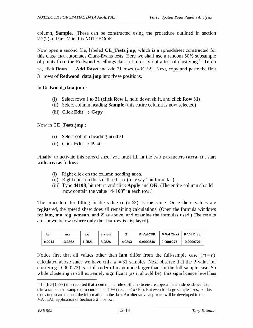
Finally, to activate this spread sheet you must fill in the two parameters (area, n), start with area as follows: (i) Right click on the column heading area. (ii) Right click on the small red box (may say “no formula”) (iii) Type 44108, hit return and click Apply and OK. (The entire column should now contain the value “44108” in each row.) The procedure for filling in the value n ( 62) is the same. Once these values are registered, the spread sheet does all remaining calculations. (Open the formula windows for lam, mu, sig, s-mean, and Z as above, and examine the formulas used.) The results are shown below (where only the first row is displayed). Notice first that all values other than lam differ from the full-sample case ( )m n calculated above since we have only 31m samples. Next observe that the P-value for clustering (.0000273) is a full order of magnitude larger than for the full-sample case. So while clustering is still extremely significant (as it should be), this significance level has 15 In [BG] (p.99) it is reported that a common a rule-of-thumb to ensure approximate independence is to take a random subsample of no more than 10% (i.e., /10m n ). But even for large sample sizes, n , this tends to discard most of the information in the data. An alternative approach will be developed in the MATLAB application of Section 3.2.5 below.

lam mu sig s-mean Z P-Val CSR P-Val Clust P-Val Disp

0.0014 13.3362 1.2521 8.2826 -4.0363 0.0000546 0.0000273 0.9999727


________________________________________________________________________ ESE 502 I.3-15 Tony E. Smith

been deflated by removing some of the positive dependencies between nn-distances. Notice also that the P-value for CSR is (by definition) exactly twice that for Clustering, and similarly that the P-value for Dispersion is exactly one minus that for Clustering. This latter P-value shows that there is no statistical evidence for Dispersion in the sense that values “as large as” 4.0363Z are almost bound to occur under CSR. 3.3.2 Analysis of Redwood Seedlings using MATLAB While the procedure in JMPIN above does allow one to take random subsamples, and thereby reduce the effect of positive dependencies among nn-distances, it only allows a single sample to be taken. So the results obtained depend to some degree on the sample selected. What one would like to do here is to take many subsamples of the same size (say with 31m ) and look at the range of Z-values obtained. If almost all samples indicate significant clustering, then this yields a much stronger result that is clearly independent of the particular sample chosen. In addition, one might for example want to use the P-value obtained for the sample mean of Z as a more representative estimate of actual significance. But to do so in JMPIN would require many repetitions of the same procedure, and would clearly be very tedious. Hence an advantage of programming languages like MATLAB is that one can easily write a program to carry out such repetitious tasks. With this in mind, we now consider an alternative approach to Clark-Evans tests using MATLAB. One should begin here by reading the notes on opening MATLAB in section 3.1 of Part IV in this NOTEBOOK. Now open MATLAB, and set the Current Directory (at the top of the MATLAB window) to the class subdirectory, T:/sys502/matlab, and open the data file, Redwoods.mat.16 The Workspace window on the left will now display the data matrices contained in this file. For example, area, is seen to be a scalar with value, 44108, that corresponds to the area value used in JMPIN above. [This number was imported from ARCMAP, and can be obtained by following the ARCMAP procedure outlined in Section 1.2(8) of Part IV.] Next consider the data matrix, Redwoods, which is seen to be a 62 x 2 matrix, with each row denoting the (x,y) coordinates of one of the 62 redwood seedlings. You can display the first three rows of this matrix by typing >> Redwoods(1:3,:). I have written a program, ce_test.m,17 in MATLAB to carry out Clark_Evans tests. You

can display this program by clicking Edit Open and selecting the file ce_test.m.18

The first few lines of this program are displayed below:

16 The extension .mat is used for data files in MATLAB. 17 The extension .m is used for all executable programs and scripts in MATLAB. 18 To view this program you can also type the command >> edit ce_test.


________________________________________________________________________ ESE 502 I.3-16 Tony E. Smith

function OUT = ce_test(pts,a,m,test) % CE_TEST.M performs the Clark-Evans tests. % % NOTE: These tests use a random subsample (size = m) of the % full sample of n nearest-neighbor distances, and % ignore edge effects. % Written by: TONY E. SMITH, 12/28/99 % INPUTS: % (i) pts = file of point locations (xi,yi), i=1..n % (ii) a = area of region % (iii) m = sample size (m <= n) % (iv) test = indicator of test to be used % 0 = two-sided test for randomness % 1 = one-sided test for clustering % 2 = one-sided test for dispersion % % OUTPUTS: OUT = vector of all nearest-neighbor distances % % SCREEN OUTPUT: critical z-value and p-value for test

The first line defines this program to be a function call ce_test, with four inputs (pts,a,n,test) and one output called OUT. The percent signs (%) on subsequent lines indicate comments intended for the reader only. The next few comment lines describe what the program does. In this case ce_test takes a subsample of size m n and performs a Clark-Evans test as in JMPIN. The next set of comment lines describe the four inputs in detail. The first, pts, contains the (x,y) coordinates of the given point pattern, and corresponds in our present case to Redwoods. The parameter a corresponds to area, and m corresponds to the number of subsamples to be taken (in this case 31m ). Finally test is an indicator denoting the type of test to be done, so that for a one-tailed test of clustering we would give test the value 1. During the execution of this program, the nearest-neighbor distance for each pattern point is calculated. Since this vector of nn-distances is useful for other applications (such as the JMPIN spread-sheet above) it is useful to save this vector. Hence the single output, OUT, is in this case the n x 1 matrix of nn-distances. The last comment line describes the screen output of this program, which in the present case is simply a display of the Z-value obtained and its corresponding P-value.


________________________________________________________________________ ESE 502 I.3-17 Tony E. Smith

To run this program, suppose that you want to save the nn-distance output as a vector called D (the names of inputs and outputs can be anything you choose). Then at the command prompt you would type: >> D = ce_test(Redwoods,area,31,1); Here it is important to end this command statement with a semicolon (;), for otherwise, all output will be displayed on the screen (in this case the contents of D). Hence by hitting return after typing the above command, the program will execute and give a screen display such as the following:

RESULTS OF TEST FOR CLUSTERING Z_Value = -3.3282 P_Value = .00043697

The results are now different from those of JMPIN above because a different random subsample of size 31m was chosen. To display the first four rows of the output vector, D, type19 >> D(1:4,:) As with the Redwoods display above, the absence of a semicolon at the end will cause the result of this command to be displayed. If you would like to save this output to your home directory (S:) as a text file, say nn_dist.txt, then use the command sequence20 >> save S:\nn_dist.txt D -ascii As was pointed out above, the results of this Clark-Evans test depend on the particular sample chosen. Hence, each time the program is run there will be a slightly different result (try it!). But in MATLAB it is a simple matter to embed ce_test in a slightly larger program that will run ce_test many times, and produce whatever summary outputs are desired. I have constructed a program to do this, called ce_test_distr.m. If you open this program you will see that it has a similar format:

19 Since D is a vector, there is only a single column. So one could simply type D(1:4) in this case. 20 To save D in another directory, say with the path description, S:\path , you must use the full command: >> save S:\path\nn_dist.txt D -ascii .


________________________________________________________________________ ESE 502 I.3-18 Tony E. Smith

function OUT = ce_test_distr(pts,a,m,test,N) % CE_TEST_DISTR.M samples ce_test.m a total of N times % Written by: TONY E. SMITH, 12/28/99 % INPUTS: % (i) pts = file of point locations (xi,yi), i=1..n % (ii) a = area of region % (iii) m = sample size (m <= n) % (iv) test = indicator of test to be used % 0 = two-sided test for randomness % 1 = one-sided test for clustering % 2 = one-sided test for dispersion % (v) N = number of sample tests. % % OUTPUTS: OUT = vector of Z-values for tests. % % SCREEN OUTPUT: (1) Normal fit of Histogram for OUT % (2) Mean of OUT % (3) P-value of mean (if normcdf present)

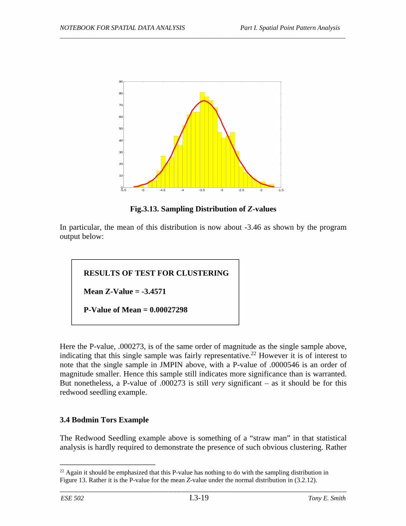
The only key difference is the new parameter, N, that specifies the number of point pattern samples of size m to be simulated (i.e., the number of times the ce_test is to be run). The output chosen for this program is the vector of Z-values obtained. So if N = 1000, then OUT will be a vector of length 1000. The screen outputs now include summary measures of this vector of Z-values, namely the histogram of Z-values in OUT, along with the mean of these Z-values and the P-value for this mean. If this program is run using the command >> Z = ce_test_distr(Redwoods,area,31,1,1000); then 1000 samples will be drawn, and the resulting Z-values will be saved in a vector, Z. In addition, a histogram of these Z-values will be displayed, as illustrated in Figure 3.13 below. Notice that the results of this simulated sampling scheme yield a distribution of Z-values that is approximately normal. While this normality property is again a consequence of the Central Limit Theorem, it should not be confused with the normal distribution in (3.2.12) upon which the Clark-Evans test is based (that requires n to be sufficiently large). However, this normality property does suggest that a 50% sample ( / 2)m n in this case yields a reasonable amount of independence among nn-distances, as it was intended to do.21

21 Hence this provides some evidence that the 10% rule of thumb in footnote 15 above is overly conservative.


________________________________________________________________________ ESE 502 I.3-19 Tony E. Smith

-5.5 -5 -4.5 -4 -3.5 -3 -2.5 -2 -1.50

10

20

30

40

50

60

70

80

90

Fig.3.13. Sampling Distribution of Z-values In particular, the mean of this distribution is now about -3.46 as shown by the program output below:

RESULTS OF TEST FOR CLUSTERING Mean Z-Value = -3.4571 P-Value of Mean = 0.00027298

Here the P-value, .000273, is of the same order of magnitude as the single sample above, indicating that this single sample was fairly representative.22 However it is of interest to note that the single sample in JMPIN above, with a P-value of .0000546 is an order of magnitude smaller. Hence this sample still indicates more significance than is warranted. But nonetheless, a P-value of .000273 is still very significant – as it should be for this redwood seedling example. 3.4 Bodmin Tors Example The Redwood Seedling example above is something of a “straw man” in that statistical analysis is hardly required to demonstrate the presence of such obvious clustering. Rather

22 Again it should be emphasized that this P-value has nothing to do with the sampling distribution in Figure 13. Rather it is the P-value for the mean Z-value under the normal distribution in (3.2.12).


________________________________________________________________________ ESE 502 I.3-20 Tony E. Smith

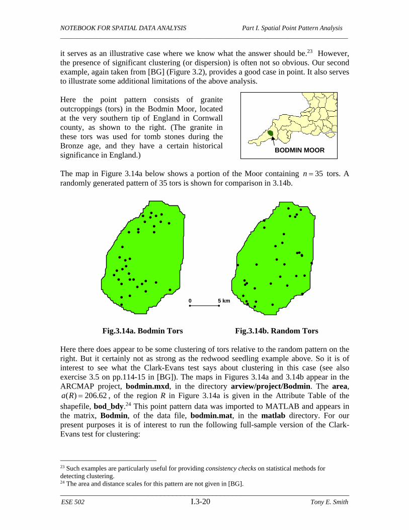
it serves as an illustrative case where we know what the answer should be.23 However, the presence of significant clustering (or dispersion) is often not so obvious. Our second example, again taken from [BG] (Figure 3.2), provides a good case in point. It also serves to illustrate some additional limitations of the above analysis. Here the point pattern consists of granite outcroppings (tors) in the Bodmin Moor, located at the very southern tip of England in Cornwall county, as shown to the right. (The granite in these tors was used for tomb stones during the Bronze age, and they have a certain historical significance in England.) The map in Figure 3.14a below shows a portion of the Moor containing 35n tors. A randomly generated pattern of 35 tors is shown for comparison in 3.14b. Fig.3.14a. Bodmin Tors Fig.3.14b. Random Tors Here there does appear to be some clustering of tors relative to the random pattern on the right. But it certainly not as strong as the redwood seedling example above. So it is of interest to see what the Clark-Evans test says about clustering in this case (see also exercise 3.5 on pp.114-15 in [BG]). The maps in Figures 3.14a and 3.14b appear in the ARCMAP project, bodmin.mxd, in the directory arview/project/Bodmin. The area,

( ) 206.62a R , of the region R in Figure 3.14a is given in the Attribute Table of the shapefile, bod_bdy.24 This point pattern data was imported to MATLAB and appears in the matrix, Bodmin, of the data file, bodmin.mat, in the matlab directory. For our present purposes it is of interest to run the following full-sample version of the Clark-Evans test for clustering:

23 Such examples are particularly useful for providing consistency checks on statistical methods for detecting clustering. 24 The area and distance scales for this pattern are not given in [BG].

BODMIN MOOR

#

# #

# #

###

#

###

#

##

##

#

###

#

# # ##

###

###

#

#

#

#

##

#

#

#

#

#

#

#

#

#

#

##

#

# #

#

#

#

#

#

#

#

#

#

#

#

#

#

#

#

#

#

0 5 km


________________________________________________________________________ ESE 502 I.3-21 Tony E. Smith

0.5 1 1.5 2 2.50

2

4

6

8

10

12

>> D = ce_test(Bodmin,area,35,1); RESULTS OF TEST FOR CLUSTERING Z_Value = -1.0346 P_Value = 0.15043 Hence even with the full sample of data points, the Clark-Evans test yields no significant clustering. Moreover, since subsampling will only act to reduce the level of significance, this tells us that there is no reason to proceed further. But for completeness, we include the following results for a subsample of size 18m (approximately 50%):25 >> ce_test_distr(Bodmin,area,18,1,1000); RESULTS OF TEST FOR CLUSTERING Mean Z-Value = -0.71318 P-Value of Mean = 0.23787 So even though there appears to be some degree of clustering, this in not detected by Clark-Evans. It turns out that there are two key theoretical difficulties here that have yet to be addressed. The first is that for point pattern samples as small as the Bodmin Tors example, the assumption of asymptotic normality may be questionable. The second is that nn-distances for points near the boundary of region R are not distributed the same as those away from the boundary. We shall consider each of these difficulties in turn. First, with respect to normality, the usual rule-of-thumb associated with the Central Limit Theorem is that sample means should be approximately normally distributed for independent random samples of size at least 30 from distributions that are not too skewed. Both of these conditions are violated in the present case. To achieve sufficient independence in the present case, subsample sizes m surely cannot be much larger that 20. Moreover, the sampling distri-bution of nn-distances in Figure 3.15 shows a definite skewness (with long right tail). This type of skewness is typical of nn-distances – even under the CSR hypothesis. [Under CSR, the theoretical distribution of nn-distances is given by the Rayleigh density in expression (2) of Section 2 in the Appendix to Part I, which is seen to have the same skewness properties.]

25 Here we are not interested in saving the Z-values, so we have specified no outputs for clust_distr.

Fig.3.15. Bodmin nn-Distances


________________________________________________________________________ ESE 502 I.3-22 Tony E. Smith

The second theoretical difficulty concerns the special nature of nn-distances near the boundary of region R. The theoretical development of the CSR hypothesis explicitly assumed that the region R is of infinite extent, so that such “edge effects” do not arise. But in practice, many point patterns of interest occur in regions R where a significant portion of the points are near the boundary of R. Recall from the discussion in Section 2.4 that if region R is viewed as a “window” through which part of a larger (stationary) point process is being observed, then points near the boundary will tend to have fewer observed neighbors than points away from the boundary. So in cases where the nearest neighbor of a point in the larger process is outside R, the observed nn-distance for that point will be greater than it should be (such as the example shown in Figure 3.16 below). Thus the distribution of nn-distances for such points will clearly have higher expected values than for interior points. For samples from CSR processes, this will tend to inflate mean nn-distances relative to their theoretical values under the CSR hypothesis. This edge effect will be demonstrated more explicitly in the next section.

Fig.3.16. Example of Edge Effect 3.5 A Direct Monte Carlo Test of CSR Given these shortcomings, we now develop a testing procedure that simulates the true distribution of nD in region R for a given pattern size, n .26 While this procedure is

computationally more intensive, it will not only avoid the need for normal approxi-mations, but will also avoid the need for subsampling altogether. The key to this procedure lies in the fact that the actual distribution of a randomly located point in R can easily be simulated on a computer. This procedure, known as rejection sampling, starts by sampling random points from rectangles. Since each rectangle is the Cartesian product of two intervals, 1 1 2 2[ , ] [ , ]a b a b , and since drawing a random number, is from an

interval [ , ]i ia b is a standard operation in any computer language, one can easily draw a

random point 1 2( , )s s s from 1 1 2 2[ , ] [ , ]a b a b . Hence for any given planar region, R, the

basic idea is to sample points from the smallest rectangle, ( )rec R containing R, and then to reject any points which are not in R.

26 Procedures for simulating distributions by random sampling are known as “Monte Carlo” procedures.

R


________________________________________________________________________ ESE 502 I.3-23 Tony E. Smith

To obtain n points in R, one continues to reject points until n are found in R. [Thus the choice of

( )rec R is designed to minimize the expected number of rejected samples.] An example for the case of Bodmin is illustrated in Figure 3.17, where for simplicity we have sampled only

10n points. Here there are seen to be four sample points that were rejected. The resulting sample points in R then constitute an independent random sample of size n that by construction must satisfy the CSR hypothesis. To see this note simply that since the larger sample in ( )rec R automatically satisfies this hypothesis, it follows that for any subset C R the probability that a point lies in C given that it is in R must have the form:

(3.5.1) Pr( ) Pr( ) ( ) / [ ( )] ( )

Pr( | )Pr( ) Pr( ) ( ) / [ ( )] ( )

C R C a C a rec R a CC R

R R a R a rec R a R

Hence expression (2.1.2) holds, and the CSR hypothesis is satisfied. More generally, for any pattern of size n one can easily simulate as many samples of size n from R as desired, and use these to estimate the sampling distribution of nD under the CSR

hypothesis. This procedure has been operationalized in the MATLAB program, clust_sim.m. Here the only additional input information required is the file of boundary points defining the Bodmin region, R . The coordinates of these boundary points are stored in the 145 x 2 matrix, Bod_poly, in the data file, bodmin.mat. To display the first three rows and last three rows of this file: first type Bod_poly(1:3,:), hit return, and type Bod_poly(143:end,:). You will then see that this matrix has the form shown to the right. Here the first row gives information about the boundary, namely that there is one polygon, and that this polygon consists of 144 points. Each subsequent row contains the (x,y) coordinates for one of these points. Notice also that the second row and the last row are identical, indicating that the polygon is closed (and thus that there are only 144 distinct points in the polygon). This boundary information for R is necessary in order to define the rectangle, ( )rec R . It is also needed to determine whether a given point in

( )rec R is also in R or not. While this latter determination seems visually evident in the present case, it turns out to be relatively complex from a programming viewpoint. A brief description of this procedure is given in section 5 of the Appendix to Part I.

Fig.3.17. Rejection Sampling

R

( )rec R

1 144 4.7 -9.7 4.4 -10.2 : : : : 5.2 -9.2 5.1 -9.2 4.7 -9.7


________________________________________________________________________ ESE 502 I.3-24 Tony E. Smith

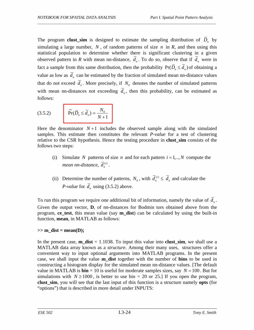
The program clust_sim is designed to estimate the sampling distribution of nD by

simulating a large number, N , of random patterns of size n in R, and then using this statistical population to determine whether there is significant clustering in a given observed pattern in R with mean nn-distance, nd . To do so, observe that if nd were in

fact a sample from this same distribution, then the probability Pr( )n nD d of obtaining a

value as low as nd can be estimated by the fraction of simulated mean nn-distance values

that do not exceed nd . More precisely, if 0N denotes the number of simulated patterns

with mean nn-distances not exceeding nd , then this probability, can be estimated as

follows:

(3.5.2) 0Pr( )1n n

ND d

N

Here the denominator 1N includes the observed sample along with the simulated samples. This estimate then constitutes the relevant P-value for a test of clustering relative to the CSR hypothesis. Hence the testing procedure in clust_sim consists of the follows two steps: (i) Simulate N patterns of size n and for each pattern 1,..,i N compute the

mean nn-distance, ( )ind .

(ii) Determine the number of patterns, 0N , with ( )i

n nd d and calculate the

P-value for nd using (3.5.2) above.

To run this program we require one additional bit of information, namely the value of nd .

Given the output vector, D, of nn-distances for Bodmin tors obtained above from the program, ce_test, this mean value (say m_dist) can be calculated by using the built-in function, mean, in MATLAB as follows: >> m_dist = mean(D); In the present case, m_dist = 1.1038. To input this value into clust_sim, we shall use a MATLAB data array known as a structure. Among their many uses, structures offer a convenient way to input optional arguments into MATLAB programs. In the present case, we shall input the value m_dist together with the number of bins to be used in constructing a histogram display for the simulated mean nn-distance values. [The default value in MATLAB is bin = 10 is useful for moderate samples sizes, say 100N . But for simulations with 1000N , is better to use bin = 20 or 25.] If you open the program, clust_sim, you will see that the last input of this function is a structure namely opts (for “options”) that is described in more detail under INPUTS:


________________________________________________________________________ ESE 502 I.3-25 Tony E. Smith

function OUT = clust_sim(poly,m,N,opts) % CLUST_SIM.M simulates the sampling distribution of average % nearest-neighbor distances in a fixed polygon. It can also determine % the P-value for a given mean nearest-neighbor distance, if supplied. % % Written by: TONY E. SMITH, 12/31/00 % INPUTS: % (i) poly = boundary file of polygon % (ii) m = number of points in polygon % (iii) N = number of simulations % (iv) opts = an (optional) structure with variable inputs: % opts.bins = number of bins in histogram (default = 10) % opts.m_dist = mean nearest-neighbor distance for testing

To define this structure in the present case, we shall use the value of m_dist just calculated, and shall set bins = 20. This is accomplished by the two commands: >> opts.m_dist = m_dist; opts.bins = 20; Notice that opts is automatically defined by simply specifying its components.27 The key point is that only the structure name, opts, needs to be specified in the command line. The program clust_sim will look to see if either of these components for opts have been specified. So if you want to use the default value of bins, just leave out this command. Moreover, if you just want to look at the histogram of simulated values (and not run a test at all), simply leave opts out of the command line. This is what is meant in the description above when opts is referred to as an “(optional) structure”. Given these preliminaries, we are now ready to run the program, clust_sim, for Bodmin. To do so, enter the command line: >> clust_sim(Bod_poly,35,1000,opts); Here we have specified n = 35 for the Bodmin case, and have specified that N = 1000 simulated patterns be constructed. The screen output will start with successive displays: percent_done = 10 percent_done = 20 : percent_done = 100

27 Note also we have put both commands on the same line to save room. Just remember to separate each command by a semicolon (;)


________________________________________________________________________ ESE 502 I.3-26 Tony E. Smith

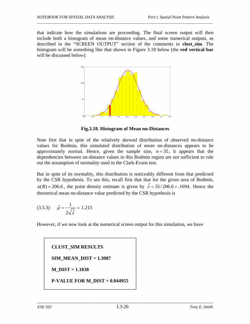
that indicate how the simulations are proceeding. The final screen output will then include both a histogram of mean nn-distance values, and some numerical outputs, as described in the “SCREEN OUTPUT” section of the comments in clust_sim. The histogram will be something like that shown in Figure 3.18 below (the red vertical bar will be discussed below):

Fig.3.18. Histogram of Mean nn-Distances Note first that in spite of the relatively skewed distribution of observed nn-distance values for Bodmin, this simulated distribution of mean nn-distances appears to be approximately normal. Hence, given the sample size, 35n , it appears that the dependencies between nn-distance values in this Bodmin region are not sufficient to rule out the assumption of normality used in the Clark-Evans test. But in spite of its normality, this distribution is noticeably different from that predicted by the CSR hypothesis. To see this, recall first that that for the given area of Bodmin,

( ) 206.6a R , the point density estimate is given by ˆ 35 / 206.6 .1694 . Hence the theoretical mean nn-distance value predicted by the CSR hypothesis is

(3.5.3) 1

ˆ 1.215ˆ2

However, if we now look at the numerical screen output for this simulation, we have

CLUST_SIM RESULTS SIM_MEAN_DIST = 1.3087 M_DIST = 1.1038 P-VALUE FOR M_DIST = 0.044955

0.8 0.9 1 1.1 1.2 1.3 1.4 1.5 1.6 1.7 1.80

50

100

150


________________________________________________________________________ ESE 502 I.3-27 Tony E. Smith

Here the first line reports the mean value of the 1000 simulated mean nn-distances. But since (by the Law of Large Numbers) a sample this large should give a fairly accurate estimate of the true mean, ( )nE D , we see that this true mean is considerably larger than

that predicted by the CSR hypothesis above.28 The key point to note here is that the edge effects depicted in Figure 3.16 above are quite significant for pattern sizes as small as

35n relative to the size of the Bodmin region, R.29 So this simulation procedure does indeed give a more accurate distribution of nn-distances in the Bodmin region under the CSR hypothesis. Observe next that the second line of screen output above gives the value of opts.m_dist as noted above (assuming this component of opts was included). The final line is the critical one, and gives the P-value for opts.m_dist, as estimated by (3.5.2) above. Hence, unlike the Clark-Evans test where no significant clustering was observed (even under full sampling), the present procedure does reveal significant clustering.30 This is shown by the position of the red vertical bar in Figure 3.18 above (at approximately a value of m_dist = 1.1038). Here there are seen to be only a few simulated values lower than m_dist. Moreover, the discussion above now shows why this result differs from Clark-Evans. In particular, by accounting for edge effects, this procedure reveals that under the CSR hypothesis, mean nn-distance values for Bodmin should be higher than those predicted by the Clark-Evans model. Hence the observed value of m_dist is actually quite low once this effect is taken into account.

28 You can convince yourself of this by running clust_sim a few times an observing that the variation in this estimated mean values is quite small. 29 Note that as the sample size n becomes larger, the expected nn-distance, ( )

nE D , for a given region, R,

becomes smaller. Hence the fraction of points sufficiently close to the boundary of R to be subject to edge effects eventually becomes small, and this edge effect disappears. 30 Note again that this P-value will change each time clust_sim is run. However, by trying a few runs you will see that all values are close to .05.

3 testing spatial randomness - penn engineeringese502/notebook/part_i/3_testing_spatial... · but...

Documents