143

143

31. COLLECTING AND PLOTTING DATA

31.1 Review/Background

So far we have discussed the physics of various reliability issues of modern

transistor such as NBTI degradation, HCI, TDDB, etc. However, in practice, we need

experimental data before making any statistical prediction about the reliability or lifetime

of the chip. The goal of this chapter is to explore about the various aspects of data

collection and the careful processing of the collected data for reliability prediction. In

particular, we will discuss how a small set of data can be transformed into a population

distribution function.

31.2 Origin of data and Statistical Inference

By the term experimental data points, we mean, for example, the failure times of

a set of transistors in case of TDDB experiment. Clearly, we cannot perform this

experiment on billions of transistors due to the cost and time constrains; still the

prediction we make based on a limited amount of data points should hold for billions of

transistors or the global population. It is then very important to construct the distribution

function from a small set of experimental data.

There are some issues regarding data collection and also dealing with datasets.

For example, in a certain situation, like acceleration-projection method, Figure. 31.1b,

one would normally explore the tail of the distribution function. However, this tail is

usually rather long and thereby entails a significant penalty in terms of cost and time if

one were to explore the function by a substantial amount of data points. Moreover, if the

initial data set is small, then any error present in the data can have serious consequences

in the final prediction. For example look at the projection voltage acceleration in

Figure. 31.1b for red and blue lines. Even though the two lines show a good agreement

144

144

for the higher acceleration voltages, using one versus the other will result in completely

wrong prediction about the time to breakdown of the transistor, note the divergence of

two lines for small voltages. Often the experimental dataset may be incomplete or non-

uniform in quality, but still we need to make best decision possible from it. Hence data

handling or the interpretation of the experimental data for making statistical inferences

are highly non trivial issues and require profound statistical theories, which we will

describe in the following sections.

31.3 Non-Parametric Information

The non-parametric information of a set of data includes quantities such as the

mean and the variance of the dataset, without making any assumption regarding the

underlying distribution function. These estimates are important to extract as much

information as possible from the raw data before fitting those data to various parametric

distribution functions. The various moments of the experimental data defined below are

the non-parametric estimates generally people are interested in

Figure. 31.1 The breakdown time of a transistor due to TDDB. (a) Shows that for

higher voltages the breakdown time is less. The non-linear projection of the

breakdown time is shown in (b) from the data obtained from the accelerated testing.

145

145

⟨�⟩ = � � ����,� �/� 31.1

�� = � � (�� −��,�⟨�⟩)�� /(� − 1) 31.2

��� = �∑ (��−< � >)�)���� − � + 1! 31.3

where N, is the number of samples. It is interesting to note that a moment of degree n,

has (N-n) in its denominator, because estimation of each parameter uses one degree of

freedom and the moments therefore must be normalized to the remaining set of

independent samples (degree of freedom).

31.4 Distribution of the Sample Statistics/Moment

Assume here we have a reference population distribution represented in

Figure. 31.2. This distribution is generated as following. Suppose we have a sample of n

devices, n is 20 in Figure. 31.2, now we run the experiment for these 20 devices which

gives us 20 data points. Then we find the average of these 20 data points, let us call this

average #. Now we repeat this procedure m times, m is 10,000 in the example of

Figure. 31.2. As a result, we will end up having 10,000 #’s, (#, #�, … , #%,%%%). Figure. 31.2 shows the distribution of these average points.

Now given a random set of 20 samples depicted by its average value as the red

arrow in Figure. 31.2, question is whether this dataset belongs to the above distribution or

not. Generally speaking, further the arrow is from the population average of the

distribution, less likely it is for the dataset to be a part of this distribution. Precisely,

however, in order to answer this question one must calculate Z-parameters of equations

31.4 and 31.5 and also P-value which is the area below the distribution from the place

where the arrow is to infinity. Then, based on the fact that larger values of P mean that

146

146

the red arrow is closer to the center of the distribution, one can decide whether this

dataset is a part of that distribution or not.

& = ' − #(√� � > 30 31.4

& = ' − #�√� � < 30 31.5

31.5 Dealing with Outliers

Sample moments are extremely sensitive to outliers and even a few such data

points can distort the estimates. These outliners may arise from …Many times due to

some unwanted reasons, (it may be noise or human error) some sample data points may

Figure. 31.2 Distribution of sample statics for the sample of size 20. The above

distribution was created by repeating the sampling for 10,000 times

147

147

be erroneous. If possible, it is prudent to repeat the experiment corresponding to that data

point; else we need to be extremely careful for the rejection of the measured data.

Main problem with averaging is that it is strongly influenced by outliers.

Outliers are those points which are distant from the rest of the data. Generally the

probability of outliers being a part of the distribution is small and the data point will

usually lies at the very extreme tail of the underlying distribution. As a result of

accounting for outliers, the average sometimes will be shift towards the outlier and give

us rather inaccurate representation of the dataset. Hence, before any manipulation of data,

one needs to exclude the outliers from parametric estimates. This can be done by using

quartile approach, which is shown in Figure. 31.3. This approach is based on not the

momentums of the dataset rather on the median therefore is not affected by the presence

of outlier. In this approach, one first needs to divide the dataset based on the median into

two sets and then divide each set, based on their median, into quartiles. Then they need to

find the inter-quartile range, IQR, which is the distance between first and forth quintiles,

median on the first and second sets. If the sample is outside of 1.5 . /01 from second

and third quintiles therefore that sample cannot be trusted and consequently cannot be

used for further analysis. This does not mean that one can ignore that sample in their

plots rather they should plot all data including outliers but don’t use them in their

analysis. Remember that every data point contains information about our measurement

and even though they should not be used for our proof of theory, they might shine light

into some details of our experiment in the future.

Figure. 31.3 Schematic showing how quintile approach works.

148

148

Figure. 31.4 schematically demonstrates why a box plot is a reliabe method to

indicate outliers without finding moments of data, remember that the moments are

affected by the outliers. As can be seen in this figure, if a data point lies outside the box,

the probability of that point being a part of the underlying distribution is so small and that

is the reason why we can put that data point aside for our following analysis, i.e. finding

average, standard deviation etc.

31.6 Removing Outliers based on Chauvenet’s Criteria

There is a well-defined prescription for the rejection of the erroneous data

known as Chauvenet’s criteria [2]. We will illustrate these criteria with a simple example

of breakdown times given in Error! Reference source not found.. According to this

prescription, we need to perform the following calculations, called Chauvenet’s criteria,

in order to decide on data rejection.

Figure. 31.4 Distribution of sample statics showing the logic behind 1.5 IQR

in Box plot. As can be seen the probability of a sample being related to the

distribition is small when it lies above 21.5/01 [1].

149

149

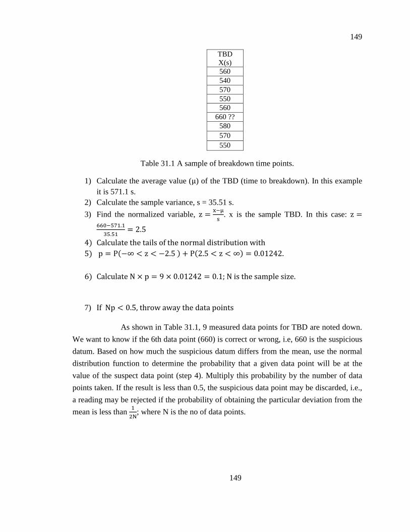
TBD X(s) 560 540 570 550 560

660 ?? 580 570 550

Table 31.1 A sample of breakdown time points.

1) Calculate the average value (μ) of the TBD (time to breakdown). In this example it is 571.1 s.

2) Calculate the sample variance, s = 35.51 s.

3) Find the normalized variable, z = 5678 . x is the sample TBD. In this case: z =99%6:;.<:.: = 2.5 4) Calculatethetailsofthenormaldistributionwith5) p = P(−∞ < z < −2.5) + P(2.5 < z < ∞) = 0.01242. 6) CalculateN . p = 9 . 0.01242 = 0.1;Nisthesamplesize.

7) IfNp < 0.5,throwawaythedatapoints As shown in Table 31.1, 9 measured data points for TBD are noted down.

We want to know if the 6th data point (660) is correct or wrong, i.e, 660 is the suspicious

datum. Based on how much the suspicious datum differs from the mean, use the normal

distribution function to determine the probability that a given data point will be at the

value of the suspect data point (step 4). Multiply this probability by the number of data

points taken. If the result is less than 0.5, the suspicious data point may be discarded, i.e.,

a reading may be rejected if the probability of obtaining the particular deviation from the

mean is less than �Y; where N is the no of data points.

150

150

31.7 Stem and Leaf Display: Pre-Histogram

In order to plot the data in the histogram, one must first dive the data points into

two groups, stem and leaf. The range of stem as shown in Figure. 31.5 can be derived

from equations 31.6 and 31.7. After finding hZ then we need to take it to the nearest

power of 10 and use it as the bases for the stem. Be sure that after doing all these steps,

your data precision should remain the same.

[ = \10 . log% ^_ 31.6

`a = b1cdaef[ g hij^k�ilmi�n��oipnhiq10 31.7

31.8 Drawing Lines Resistant to Outliers

If your data points have outliers, then plotting a line using regular techniques

will result in conclusion, which is corrupted by the outliers and can be misleading. In

Figure. 31.5 An example of stem and leaf for an arbitary set of data shown

above. [~13 and ̀ a = 4.7 and therefore is 10. That is the reason why stems

are a products of 10.

151

151

order to draw a line resistant to outliers one needs to follow the method described in the

following example.

Suppose we have a dataset, 9 data points in Figure. 31.6. In order to avoid the

effect of outliers, we first divide data into three different groups following procedures in

Table 31.2. Then, we will find the median of each group, for both data points in x-axis

and also y-axis i.e. (tu , vu), (tw, vw), (tx , vx). Now that we have the median of each

group, we can draw a line between those three medians instead of original data points.

This line, as a result, will not have any effect from outliers.

Number of data points (n) Dividing procedure

n=3k k, k, k

n=3k +1 k, k+1, k

n=3k+2 k+1, k, k+1

Table 31.2 Calculation with Hazen formula for censored and uncensored data.

Figure. 31.6 Schematic representing an effective method to plot a line resistant to

outliers.

152

152

31.9 Plotting of Data

Suppose we have 5 transistors and we have measured the 5 break down times for those transistors. Now if we want to plot the Cumulative distribution function (F) of the

breakdown times, we can use either Fz = zZ . or Fz = zZ{ . We can immediately see

there is a problem with first form. Wheni = n, Fz = 1 and the Weibull distribution function W = ln(− ln(1 − Fz)) blows up. Hence the second functional form is preferred for plotting the CDF.

There is however one more problem associated with the arrival time distribution

around each breakdown time point (shown as yellow region in Figure. 31.7). To explain this, let us assume we have a population of 25 transistors, and we need to represent the cumulative breakdown time distribution with a sample of 5 transistors only. This

situation is illustrated in Figure. 31.8. If we use the simple formula Fz = zZ or Fz = z6Z

then some population data points will exactly match with the sample data points but the maximum error between the sample and the population data points will be very high. The

Figure. 31.7 The discrete breakdown times for the sample of 5 transistors and the

corresponding CDF.

153

153

error can be minimized by using a new formula for the CDF based on median of the sample data points can be used. This formula is shown in equation 31.8 and it is also known as Hazen formula.

}wf~�da,� = � − �^ − 2� + 1(� = 0.3) 31.8

In order to derive Hazen formula [2], let p be the probability that breakdown

time is less than or equal to ��� sample time. If there is n sample data points, then the probability that population data value is less than ��� sample time is

� = ( )�a o�(1 − o)a6� 31.9

Hence

Figure. 31.8 CDF of the population of 25 transistors and a sample of 5

transistors. CDF derived from the Hazen formula minimizes the maximum

error between the population and the sample.

154

154

� = k�ko = �( )�a o�6(1 − o)a6� 31.10

Since

� �ko�������,�% = 12 31.11

}�f~�da,� = � − �^ − 2� + 1(� = 0.3) 31.12

We see in Figure. 31.8 that the maximum error between the CDF of total population and the CDF of sample of 5 transistors is a minimum for the case of Hazen formula.

31.10 Handling Censored Data

So far we have discussed outliers in dataset and how to detect and exclude them

from our analysis. Aside from outliers, there is another type of data called censored data

which also needs be to identified and treated carefully during data analyzing step.

Censored data, in this context, refers to a data point where due to human error, instrument

malfunction, etc one experiment was not complete or was missing while the others were

complete and accurate. In this case, throwing away the incomplete experiment result or

data point will result in inaccurate projection of data. In order to understand what

censored data is and how we should deal with them, let us look at the following example.

Suppose we have a sample of 5 transistors and we want to plot the CDF of the

breakdown times of those transistors. If due to some reasons one sample data point is

missing, how can we still make the best decision out of the remaining sample data points.

In order to do so we need to be very careful in post processing of the remaining data (also

155

155

known as censored data). We will illustrate this with the following simple example

shown in Figure. 31.9.

Uncensored Data

(Hazen formula with α=0)

Censored Data (third data point is missing)

(Hazen formula with α=0)

F1 = 1/6 F1 = 1/5

F2 = 2/6 F2 = 2/5

F3 = 3/6 F3 = 2/5

F4 = 4/6 F4 = 3/5

F5 = 5/6 F5 = 4/5

Table 31.3 Calculation with Hazen formula for censored and uncensored data.

If all the 5 sample data points were present, then the CDF is plotted with the blue line in Figure. 31.9, with the Hazen formula (α = 0) as shown in Table 31.1. Now,

t

Fi

One Sample is missing

0 1 2 3 4 50

0.2

0.4

0.6

0.8

1

; 41

in

n=

+

; 51

in

n=

+

Kaplan-Meier

t

Fi

One Sample is missing

0 1 2 3 4 50

0.2

0.4

0.6

0.8

1

; 41

in

n=

+

; 51

in

n=

+

Kaplan-Meier

0 1 2 3 4 50

0.2

0.4

0.6

0.8

1

; 41

in

n=

+

; 51

in

n=

+

Kaplan-Meier

Figure. 31.9 CDF of censored and uncensored data.

156

156

let us assume the third sample is missing. In this case one can still use the Hazen formula with the 4 data points again presented in Table 31.3 and plotted in Figure. 31.9 with the red dashed line. We immediately see that there is a problem in this approach. Since the third sample is missing, that means the CDF for the first and second data points should not be affected. But with the Hazen formula, we see the first and second data points also get affected. In other words, if we use Hazen formula for censored data, then past data points are affected by the future missing data points, which is not desirable. To eradicate this problem, Kaplan-Meier Formula is used for plotting of the censored data and the formula is given by

}� = 1 − � ^ − � + 1^ − 2� + 1���^�� + 1 − �^�� + 2 − ����� 31.13

For � = 0;

}� = 1 −��^�� + 1^�� + 2���� 31.14

This Formula is applicable for both the censored as well as uncensored data. We illustrate this with in the followings.

31.11 Kaplan–Meier Formula for Uncensored Data

nsi before ti

5 4 3 2 1

nsi after ti

4 3 2 1 0

Table 31.4 value of n for set of data.

According to the Kaplan –Meier formula the CDF values are:

} = 1 − 4 + 14 + 2 = 16 31.15

157

157

}� = 1 − 4 + 14 + 2 . 3 + 13 + 2 = 26 31.16

}< = 1 − 4 + 14 + 2 . 3 + 13 + 2 . 2 + 12 + 2 = 36 31.17

}� = 1 − 4 + 14 + 2 . 3 + 13 + 2 . 2 + 12 + 2 . 1 + 11 + 2 = 46 31.18

}: = 1 − 4 + 14 + 2 . 3 + 13 + 2 . 2 + 12 + 2 . 1 + 11 + 2 . 0 + 10 + 2 = 56 31.19

These values are different from those obtained by the Hazen formula for

censored data. We note that in this case the first and second sample data points are not

affected by that of the missing data point.

We can summarize the results for the CDF for the case of censored data with the

Table 31.5

Method T=1 T=2 T=3 T=4 T=5

Hazen Formula 1/6 2/6 3/6 4/6 5/6

Hazen formula with

one sample missing

1/5 2/5 Missing 3/5 4/5

Kaplan –Meier

Formula

1/6 2/6 Missing 5/9 7/9

Table 31.5 Summary of CDFs derived using different formulas for censored dara.

31.12 Conclusions

Generation of the experimental data is costly both in terms of time and

equipment and hence careful treatment in analyzing the data is very important. Simple

non-parametric estimates like mean, standard deviation, median, etc. are very useful

158

158

indicators for the corresponding quantities of the whole population space and they also

help in selecting the appropriate distribution function. Non-parametric plotting of the

distribution function gives important insight about the population but the plotting

approaches for the censored and uncensored data are very different. Finally, a good

parametric fit of the sample data allows one to estimate the tails of the distribution

correctly. We will discuss the details of the fitting algorithms as well as the ‘goodness-of-

fit’ of the distributions in next chapters.

References

[1] D. C. Hoaglen, F. Mosteller, and J.W. Tukey, “Understanding Robust and Exploratory Data Analysis”, Wiley Interscience, 1983. Explains the importance of Median based analysis when the dataset is small and the quality cannot be guaranteed.

[2] Les Kirkup, “Data Analysis with Excel”, Cambridge University Press, p. 185. [3] Ross, 1999 Conf. on Elec. Insulation/Dielectric Phenomena, p. 170; Ohring, p. 223.

[4] L. Wolstenholme, Reliability Modeling: A Statistical Approach, Chapman&Hall/CRC Press, 1999. 2. [5] R. H. Myers and D.C. Montgomery, “Response Surface Methodology”, Wiley Interscience, 2002.