31 kinematical and dynamical models of kr 6 kuka robot ...cdn.intechweb.org/pdfs/10640.pdf · kr6...
TRANSCRIPT

Kinematical and Dynamical Models of KR 6 KUKA Robot, including the kinematic control in a parallel processing platform 601
Kinematical and Dynamical Models of KR 6 KUKA Robot, including the kinematic control in a parallel processing platform
John Faber Archila Díaz, Max Suell Dutra and Fernando Augusto de Noronha Castro Pinto
x
Kinematical and Dynamical Models of KR 6 KUKA Robot, including the kinematic control in
a parallel processing platform
John Faber Archila Díaz Universidad Industrial de Santander. UIS
Colombia Max Suell Dutra and Fernando Augusto de Noronha Castro Pinto
Universidade Federal do Rio de Janeiro, UFRJ Brazil
1. Introduction
This chapter presents the study and modelling of KR 6 KUKA Robot, of the Robotics Laboratory, Federal University of Rio de Janeiro, see fig 1. The chapter shows the CAD model (Computer Aided Design), the direct kinematics, the inverse kinematics and the inverse dynamical model. The direct kinematic is based in the use of homogeneous matrix. The inverse kinematics uses the quadratic equations model. The dynamical model is based on the use of Euler-Lagrange equations, using the D-H (Denavit-Hartenberg) algorithm and taking into account the inertia tensor, which was found with help of CAE tools (Computer Aided Engineering), On the other hand the Jacobian of robot manipulator is present, it‘s necessary for the kinematic control. The chapter finishes with the implementation of the inverse kinematic in one parallel processing platform and analyzes its performance.
Fig. 1. KR 6 KUKA Robot, Robotics Laboratory, Federal University of Rio de Janeiro UFRJ.
31
www.intechopen.com
Robot Manipulators, New Achievements602
Z
X
Y
PPx
Pz
Py
W
V
U
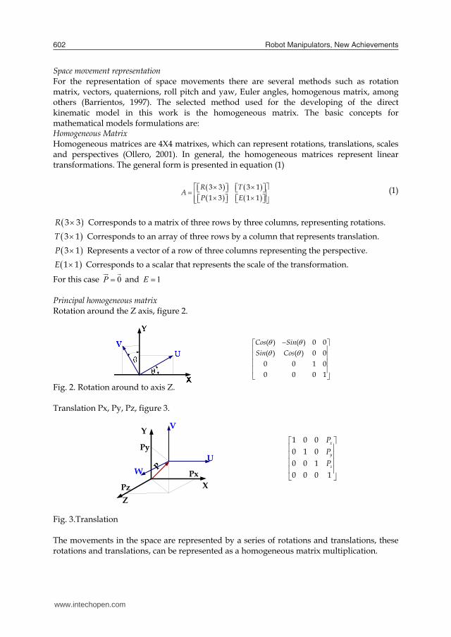
Space movement representation For the representation of space movements there are several methods such as rotation matrix, vectors, quaternions, roll pitch and yaw, Euler angles, homogenous matrix, among others (Barrientos, 1997). The selected method used for the developing of the direct kinematic model in this work is the homogeneous matrix. The basic concepts for mathematical models formulations are: Homogeneous Matrix Homogeneous matrices are 4X4 matrixes, which can represent rotations, translations, scales and perspectives (Ollero, 2001). In general, the homogeneous matrices represent linear transformations. The general form is presented in equation (1)
3 3 3 11 3 1 1
R TA
P E (1)
3 3R Corresponds to a matrix of three rows by three columns, representing rotations.
3 1T Corresponds to an array of three rows by a column that represents translation.
3 1P Represents a vector of a row of three columns representing the perspective.
1 1E Corresponds to a scalar that represents the scale of the transformation.
For this case 0 P and 1E
Principal homogeneous matrix Rotation around the Z axis, figure 2.
( ) ( ) 0 0( ) ( ) 0 0
0 0 1 00 0 0 1
Cos SinSin Cos
Fig. 2. Rotation around to axis Z. Translation Px, Py, Pz, figure 3.
1 0 00 1 00 0 10 0 0 1
x
y
z
PPP
Fig. 3.Translation The movements in the space are represented by a series of rotations and translations, these rotations and translations, can be represented as a homogeneous matrix multiplication.
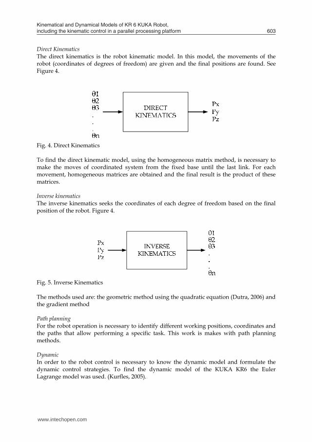
Direct Kinematics The direct kinematics is the robot kinematic model. In this model, the movements of the robot (coordinates of degrees of freedom) are given and the final positions are found. See Figure 4.
Fig. 4. Direct Kinematics To find the direct kinematic model, using the homogeneous matrix method, is necessary to make the moves of coordinated system from the fixed base until the last link. For each movement, homogeneous matrices are obtained and the final result is the product of these matrices. Inverse kinematics The inverse kinematics seeks the coordinates of each degree of freedom based on the final position of the robot. Figure 4.
Fig. 5. Inverse Kinematics The methods used are: the geometric method using the quadratic equation (Dutra, 2006) and the gradient method Path planning For the robot operation is necessary to identify different working positions, coordinates and the paths that allow performing a specific task. This work is makes with path planning methods. Dynamic In order to the robot control is necessary to know the dynamic model and formulate the dynamic control strategies. To find the dynamic model of the KUKA KR6 the Euler Lagrange model was used. (Kurfles, 2005).
www.intechopen.com
Kinematical and Dynamical Models of KR 6 KUKA Robot, including the kinematic control in a parallel processing platform 603
Z
X
Y
PPx
Pz
Py
W
V
U
Space movement representation For the representation of space movements there are several methods such as rotation matrix, vectors, quaternions, roll pitch and yaw, Euler angles, homogenous matrix, among others (Barrientos, 1997). The selected method used for the developing of the direct kinematic model in this work is the homogeneous matrix. The basic concepts for mathematical models formulations are: Homogeneous Matrix Homogeneous matrices are 4X4 matrixes, which can represent rotations, translations, scales and perspectives (Ollero, 2001). In general, the homogeneous matrices represent linear transformations. The general form is presented in equation (1)
3 3 3 11 3 1 1
R TA
P E (1)
3 3R Corresponds to a matrix of three rows by three columns, representing rotations.
3 1T Corresponds to an array of three rows by a column that represents translation.
3 1P Represents a vector of a row of three columns representing the perspective.
1 1E Corresponds to a scalar that represents the scale of the transformation.
For this case 0 P and 1E
Principal homogeneous matrix Rotation around the Z axis, figure 2.
( ) ( ) 0 0( ) ( ) 0 0
0 0 1 00 0 0 1
Cos SinSin Cos
Fig. 2. Rotation around to axis Z. Translation Px, Py, Pz, figure 3.
1 0 00 1 00 0 10 0 0 1
x
y
z
PPP
Fig. 3.Translation The movements in the space are represented by a series of rotations and translations, these rotations and translations, can be represented as a homogeneous matrix multiplication.
Direct Kinematics The direct kinematics is the robot kinematic model. In this model, the movements of the robot (coordinates of degrees of freedom) are given and the final positions are found. See Figure 4.
Fig. 4. Direct Kinematics To find the direct kinematic model, using the homogeneous matrix method, is necessary to make the moves of coordinated system from the fixed base until the last link. For each movement, homogeneous matrices are obtained and the final result is the product of these matrices. Inverse kinematics The inverse kinematics seeks the coordinates of each degree of freedom based on the final position of the robot. Figure 4.
Fig. 5. Inverse Kinematics The methods used are: the geometric method using the quadratic equation (Dutra, 2006) and the gradient method Path planning For the robot operation is necessary to identify different working positions, coordinates and the paths that allow performing a specific task. This work is makes with path planning methods. Dynamic In order to the robot control is necessary to know the dynamic model and formulate the dynamic control strategies. To find the dynamic model of the KUKA KR6 the Euler Lagrange model was used. (Kurfles, 2005).
www.intechopen.com

Robot Manipulators, New Achievements604
2. Modelling
For the Robot modelling, CAD models and mathematical models were developed. The mathematical models are for the kinematics and dynamics of the manipulator and are presented below.
2.1 CAD Model The Figure 6 shows the model developed in the CAD software Solid Edge®, based on the KR6 KUKA Robot of Robotics Laboratory at UFRJ, taking into account its main geometric characteristics.
Fig. 6. CAD model of the KR6 KUKA Robot
2.2 Direct Kinematics The manipulator kinematics model is based on the use of homogeneous matrix for this purpose; coordinated systems are located in a convention proposed by the authors. Supported by recommendations of the Denavit-Hartenberg algorithm (Denavit & Hartenberg, 1955). The convention adopted is:
On the spin axis of each joint, locate the z-axis direction such that positive rotations are counter clockwise. See Figure 7.
The x-axis is located parallel to each link, oriented to the follow coordinate system. See Figure 7.
Fig. 7. Reference coordinate systems, for the KR6 KUKA Robot. The proposed convention, seeks to define all positive rotations of joints when the rotation direction is counter clockwise and to make the translations always on the x-axis in positive direction. The generated movements for going from one frame to another are mathematically represented by homogeneous matrix transformations and follow the particular geometry of the robot link to link:
1. R(Zo,θo)*T(Zo,L1) 2. T(Xo´,L2)*R(Xo´,π/2)*R(Zo´, π/2) 3. R(Z1,θ1)*T(X1,L3) *R(Z1´, -π/2) 4. R(Z2,θ2)*T(X2,L4)
The full kinematic model is presented in equation (2):
'0 1 2
' '1 1
'1 3 1 2 2
2 4
, , ,
, , ,2 2
, , ,2
,
o o o
o o
T R Z T Z L T X L
R X R Z R Z
T X L R Z R Z
T X L
(2)
2.2 Inverse Kinematics To obtain the inverse kinematic model the geometry of the robot is used, using the quadratic equation method (Dutra, 2006), obtaining the solution for different configurations of the
www.intechopen.com

Kinematical and Dynamical Models of KR 6 KUKA Robot, including the kinematic control in a parallel processing platform 605
2. Modelling
For the Robot modelling, CAD models and mathematical models were developed. The mathematical models are for the kinematics and dynamics of the manipulator and are presented below.
2.1 CAD Model The Figure 6 shows the model developed in the CAD software Solid Edge®, based on the KR6 KUKA Robot of Robotics Laboratory at UFRJ, taking into account its main geometric characteristics.
Fig. 6. CAD model of the KR6 KUKA Robot
2.2 Direct Kinematics The manipulator kinematics model is based on the use of homogeneous matrix for this purpose; coordinated systems are located in a convention proposed by the authors. Supported by recommendations of the Denavit-Hartenberg algorithm (Denavit & Hartenberg, 1955). The convention adopted is:
On the spin axis of each joint, locate the z-axis direction such that positive rotations are counter clockwise. See Figure 7.
The x-axis is located parallel to each link, oriented to the follow coordinate system. See Figure 7.
Fig. 7. Reference coordinate systems, for the KR6 KUKA Robot. The proposed convention, seeks to define all positive rotations of joints when the rotation direction is counter clockwise and to make the translations always on the x-axis in positive direction. The generated movements for going from one frame to another are mathematically represented by homogeneous matrix transformations and follow the particular geometry of the robot link to link:
1. R(Zo,θo)*T(Zo,L1) 2. T(Xo´,L2)*R(Xo´,π/2)*R(Zo´, π/2) 3. R(Z1,θ1)*T(X1,L3) *R(Z1´, -π/2) 4. R(Z2,θ2)*T(X2,L4)
The full kinematic model is presented in equation (2):
'0 1 2
' '1 1
'1 3 1 2 2
2 4
, , ,
, , ,2 2
, , ,2
,
o o o
o o
T R Z T Z L T X L
R X R Z R Z
T X L R Z R Z
T X L
(2)
2.2 Inverse Kinematics To obtain the inverse kinematic model the geometry of the robot is used, using the quadratic equation method (Dutra, 2006), obtaining the solution for different configurations of the
www.intechopen.com

Robot Manipulators, New Achievements606
robot in closed form. The first step is to characterize the robot in a vectorial model, for any position, see Figure 8.
Fig. 8. Vectorial model for inverse kinematics. Based on the figure 8, the vector sum is developed and the algebraic equations for each joint are obtained: For the joint 1 equation (3)
2
11
42
B B ACSinA
(3)
Were 2 2 2 2
4 3D L L X Z
2 2 2 23 3
32 2 2
3
4 44
4
A X L Z LB ZL DC D X L
(4)
For the joint 2 equation (5)
2
12 1
42
b b acSina
(5)
were:
2 2 2 23 4
2 2 2 24 4
42 2 2
4
4 44
4
d L L X Za X L Z Lb ZL Dc d X L
(6)
The above equations, equation (3) to equation (6), represent the inverse kinematic model in closed form and providing solutions for different settings of KR 6 KUKA Robot in the workspace.
2.3 Numerical method to the inverse kinematics For the implementation of inverse kinematic model in a parallel processing platform, the gradient method was proposed in order to observe the platform potential for the application in the control of the manipulator. The general form of the method corresponds to equation (7)
11 ( ) ( )n n n nJ f (7)
Were 1( )nJ correspond to inverse jacobian of the robot, which can be seen in equation (8) and the functions ( )nf depends of kinematical direc model, equation (9)
1 1 1
1 2 3
2 2 2
1 2 3
3 3 3
1 2 3
( ) ( ) ( )
( ) ( ) ( ) ( )( )
( ) ( ) ( )
in
j
f f f
f f f fJ
f f f
(8)
1 1 2 3 1
2 1 2 3 2
3 1 2 3 3
( , , )( , , )( , , )
f af af a
(9)
According to the equations (8) and (9), it is necessary to determine the Jacobian of the robot and develop the algorithm to find the corresponding angles for each position of the manipulator, the functions of equations (9) are made explicit in the set of equations (10):
1 2 0
3 1 0
4 1 2 0
2 2 0
3 1 0
4 1 2 0
3 1 3 1
4 1 2
( )( ) ( )
( ( ) ( )( )
( ) ( )( ) ( )
( )( )
o
o
o
f L CosL Cos CosL Cos Cos X
f L SenoL Cos SenoL Cos Seno Y
f L L SenoL Seno Z
(10)
The equations (10), correspond to the solution for the direct kinematics of the robot.
2.4 Inverse Dynamic The dynamic model is based on the Euler Lagrange equations (11). Specifically in the model presented by Fu (1987), it considers the inertial effects of the manipulator by means of the
www.intechopen.com

Kinematical and Dynamical Models of KR 6 KUKA Robot, including the kinematic control in a parallel processing platform 607
robot in closed form. The first step is to characterize the robot in a vectorial model, for any position, see Figure 8.
Fig. 8. Vectorial model for inverse kinematics. Based on the figure 8, the vector sum is developed and the algebraic equations for each joint are obtained: For the joint 1 equation (3)
2
11
42
B B ACSinA
(3)
Were 2 2 2 2
4 3D L L X Z
2 2 2 23 3
32 2 2
3
4 44
4
A X L Z LB ZL DC D X L
(4)
For the joint 2 equation (5)
2
12 1
42
b b acSina
(5)
were:
2 2 2 23 4
2 2 2 24 4
42 2 2
4
4 44
4
d L L X Za X L Z Lb ZL Dc d X L
(6)
The above equations, equation (3) to equation (6), represent the inverse kinematic model in closed form and providing solutions for different settings of KR 6 KUKA Robot in the workspace.
2.3 Numerical method to the inverse kinematics For the implementation of inverse kinematic model in a parallel processing platform, the gradient method was proposed in order to observe the platform potential for the application in the control of the manipulator. The general form of the method corresponds to equation (7)
11 ( ) ( )n n n nJ f (7)
Were 1( )nJ correspond to inverse jacobian of the robot, which can be seen in equation (8) and the functions ( )nf depends of kinematical direc model, equation (9)
1 1 1
1 2 3
2 2 2
1 2 3
3 3 3
1 2 3
( ) ( ) ( )
( ) ( ) ( ) ( )( )
( ) ( ) ( )
in
j
f f f
f f f fJ
f f f
(8)
1 1 2 3 1
2 1 2 3 2
3 1 2 3 3
( , , )( , , )( , , )
f af af a
(9)
According to the equations (8) and (9), it is necessary to determine the Jacobian of the robot and develop the algorithm to find the corresponding angles for each position of the manipulator, the functions of equations (9) are made explicit in the set of equations (10):
1 2 0
3 1 0
4 1 2 0
2 2 0
3 1 0
4 1 2 0
3 1 3 1
4 1 2
( )( ) ( )
( ( ) ( )( )
( ) ( )( ) ( )
( )( )
o
o
o
f L CosL Cos CosL Cos Cos X
f L SenoL Cos SenoL Cos Seno Y
f L L SenoL Seno Z
(10)
The equations (10), correspond to the solution for the direct kinematics of the robot.
2.4 Inverse Dynamic The dynamic model is based on the Euler Lagrange equations (11). Specifically in the model presented by Fu (1987), it considers the inertial effects of the manipulator by means of the
www.intechopen.com

Robot Manipulators, New Achievements608
inertia tensor. The use of the transformation matrices is an advantage by the fact that its derivatives can be obtained as a linear combination of a constant matrix multiplied by the original matrix.
i
i i
d L LTdt
(11)
were: L corresponds to the Lagrangian (kinetic energy less potential energy) equation (12) ( ), ( ) ( ), ( ) -U (t) L t t K t t (12)
The model proposed by Fu (1987) is presented in equation (13)
1 1 1
n n n
i ik k ikm k m ik k m
T D h c (13)
The model represented in a matrix form is shown in equation (14)
( ) ( ( )) ( ) ( ( ), ( )) ( ( ))T t D t t h t t c t (14) were: 1 2( ) ( ) ( ) ...... ( ) T
nT t T t T t T t Vector torque, size nx1.
1 2( ) ( ) ( ) ...... ( ) Tnt t t t Vector of joint positions, size nx1.
1 2( ) ( ) ( ) ...... ( )
T
nt t t t Vector of angular Velocities, size nx1.
1 2( ) ( ) ( ) ...... ( )
T
nt t t t Vector of angular acceleration, size nx1.
max( , )
, 1,2,....,n
Tik jk j ji
j i kD Tr U J U i k n Inertia matrix, size nxn
2
2
2
xx yy zzxy xz i i
xx yy zzxy yz i i
i
xx yy zzxz yz i i
i i i i i i i
I I II I m x
I I II I m yJ
I I II I m z
m x m y m z m
(15) Inertia Tensor, size 4x4.
1 2( , ) ...... T
nh h h h Vector of Coriolis and centrifugal force, Size nx1
1 1
1,2,....,n n
i ikm k mk m
h h i n
max( , , )
, , 1,2,....,n
Tikm jkm j ji
j i k mh Tr U J U i k m n
1 1
1,2,....,n n
i ikm k mk m
h h i n
1 2( ) ...... Tnc c c c Gravity forces vector size nx1
1,2,....,n
ji j ji j
j ic m gU r i n
From the direct kinematic model, presented in equation (2), is applied the model of Fu , to which is necessary determine Ujk matrices, the inertia tensor Ji for each link, the inertia effects D, the matrix hi and hijk of Coriolis and centrifugal acceleration, the position vector R and the gravitational vectors force C. To calculate the matrix Ujk is used the canonical equation (16):
010
1j j
jk j i kk
AU A Q A (16)
To determine the inertia tensor of each link the CAD model was used, obtaining the inertia moments around of the reference system used in the assembly module of the CAD software. As an example is presented the case of link 2, the software presents the inertia in the way shown in Figure 8.
Fig. 8. Inertia obtained in Solid Edge®. The Table 1 was obtained using the software solid edge®, showing data of inertia and centroids.
m2 38,767 Kg Ixx2 112,0126 Kg-m2 Iyy2 107,2872 Kg-m2 Izz2 16 Kg-m2
www.intechopen.com

Kinematical and Dynamical Models of KR 6 KUKA Robot, including the kinematic control in a parallel processing platform 609
inertia tensor. The use of the transformation matrices is an advantage by the fact that its derivatives can be obtained as a linear combination of a constant matrix multiplied by the original matrix.
i
i i
d L LTdt
(11)
were: L corresponds to the Lagrangian (kinetic energy less potential energy) equation (12) ( ), ( ) ( ), ( ) -U (t) L t t K t t (12)
The model proposed by Fu (1987) is presented in equation (13)
1 1 1
n n n
i ik k ikm k m ik k m
T D h c (13)
The model represented in a matrix form is shown in equation (14)
( ) ( ( )) ( ) ( ( ), ( )) ( ( ))T t D t t h t t c t (14) were: 1 2( ) ( ) ( ) ...... ( ) T
nT t T t T t T t Vector torque, size nx1.
1 2( ) ( ) ( ) ...... ( ) Tnt t t t Vector of joint positions, size nx1.
1 2( ) ( ) ( ) ...... ( )
T
nt t t t Vector of angular Velocities, size nx1.
1 2( ) ( ) ( ) ...... ( )
T
nt t t t Vector of angular acceleration, size nx1.
max( , )
, 1,2,....,n
Tik jk j ji
j i kD Tr U J U i k n Inertia matrix, size nxn
2
2
2
xx yy zzxy xz i i
xx yy zzxy yz i i
i
xx yy zzxz yz i i
i i i i i i i
I I II I m x
I I II I m yJ
I I II I m z
m x m y m z m
(15) Inertia Tensor, size 4x4.
1 2( , ) ...... T
nh h h h Vector of Coriolis and centrifugal force, Size nx1
1 1
1,2,....,n n
i ikm k mk m
h h i n
max( , , )
, , 1,2,....,n
Tikm jkm j ji
j i k mh Tr U J U i k m n
1 1
1,2,....,n n
i ikm k mk m
h h i n
1 2( ) ...... Tnc c c c Gravity forces vector size nx1
1,2,....,n
ji j ji j
j ic m gU r i n
From the direct kinematic model, presented in equation (2), is applied the model of Fu , to which is necessary determine Ujk matrices, the inertia tensor Ji for each link, the inertia effects D, the matrix hi and hijk of Coriolis and centrifugal acceleration, the position vector R and the gravitational vectors force C. To calculate the matrix Ujk is used the canonical equation (16):
010
1j j
jk j i kk
AU A Q A (16)
To determine the inertia tensor of each link the CAD model was used, obtaining the inertia moments around of the reference system used in the assembly module of the CAD software. As an example is presented the case of link 2, the software presents the inertia in the way shown in Figure 8.
Fig. 8. Inertia obtained in Solid Edge®. The Table 1 was obtained using the software solid edge®, showing data of inertia and centroids.
m2 38,767 Kg Ixx2 112,0126 Kg-m2 Iyy2 107,2872 Kg-m2 Izz2 16 Kg-m2
www.intechopen.com

Robot Manipulators, New Achievements610
Ixy2 7,1702 Kg-m2 Ixz2 -22,7151 Kg-m2 Iyz2 -30,4911 Kg-m2 Xc -0,3661 M Yc -0,505 M Zc 1,55 m
Table 1. Inertial and centroidal data for link two. To obtain the inertia tensor, equation (15), it is necessary to make two changes to the inertia tensor data obtained with solid edge®. The first change is a translation of the reference base system to the reference of the joint and the second change is to orient the base reference system according to the reference system selected in the kinematic model. Figure 9
XY
Z
X1Y1
Z1
Z2 X2
Fig. 9. Reference system for link two To the translation of the references systems it is necessary to apply the Steiner theorem (Beer, 1980), the distances to apply the theorem are presented in Table 2
X axis2 0 M Y axis2 -0,505 M Z axis2 1,35 M
Table 2. Distances to Steiner theorem application. The inertia tensor for the link two after making changes based on the equation (15) is presented in Table 3
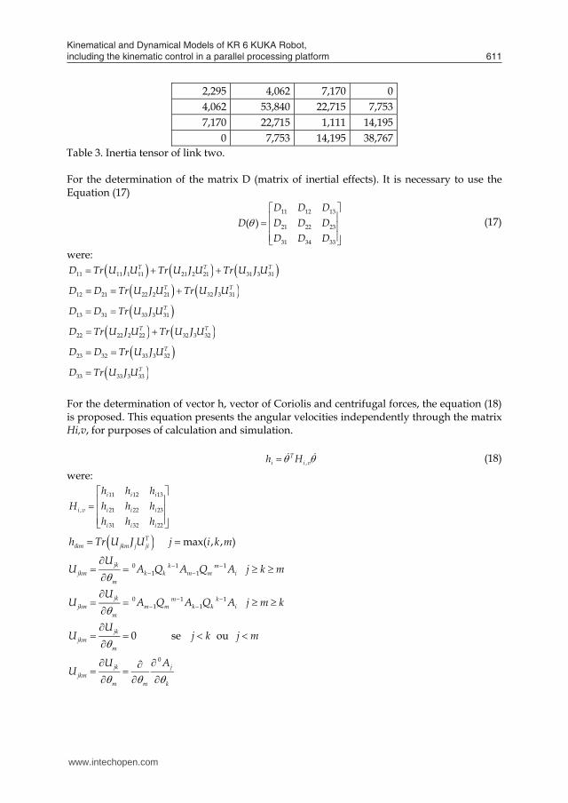
2,295 4,062 7,170 0 4,062 53,840 22,715 7,753 7,170 22,715 1,111 14,195
0 7,753 14,195 38,767 Table 3. Inertia tensor of link two. For the determination of the matrix D (matrix of inertial effects). It is necessary to use the Equation (17)
11 12 13
21 22 23
31 34 33
( )D D D
D D D DD D D
(17)
were: 11 11 1 11 21 2 21 31 3 31T T TD Tr U J U Tr U J U Tr U J U
12 21 22 2 21 32 3 31T TD D Tr U J U Tr U J U
13 31 33 3 31TD D Tr U J U
22 22 2 22 32 3 32T TD Tr U J U Tr U J U
23 32 33 3 32TD D Tr U J U
33 33 3 33TD Tr U J U
For the determination of vector h, vector of Coriolis and centrifugal forces, the equation (18) is proposed. This equation presents the angular velocities independently through the matrix Hi,v, for purposes of calculation and simulation.
,
Ti i vh H (18)
were:
11 12 13
, 21 22 23
31 32 22
i i i
i v i i i
i i i
h h hH h h h
h h h
max( , , )Tikm jkm j jih Tr U J U j i k m
0 1 1
1 1 jk k mjkm k k m m i
m
UU A Q A Q A j k m
0 1 1
1 1 jk m kjkm m m k k i
m
UU A Q A Q A j m k
0 se ou jk
jkmm
UU j k j m
0jk j
jkmm m k
U AU
www.intechopen.com
Kinematical and Dynamical Models of KR 6 KUKA Robot, including the kinematic control in a parallel processing platform 611
Ixy2 7,1702 Kg-m2 Ixz2 -22,7151 Kg-m2 Iyz2 -30,4911 Kg-m2 Xc -0,3661 M Yc -0,505 M Zc 1,55 m
Table 1. Inertial and centroidal data for link two. To obtain the inertia tensor, equation (15), it is necessary to make two changes to the inertia tensor data obtained with solid edge®. The first change is a translation of the reference base system to the reference of the joint and the second change is to orient the base reference system according to the reference system selected in the kinematic model. Figure 9
XY
Z
X1Y1
Z1
Z2 X2
Fig. 9. Reference system for link two To the translation of the references systems it is necessary to apply the Steiner theorem (Beer, 1980), the distances to apply the theorem are presented in Table 2
X axis2 0 M Y axis2 -0,505 M Z axis2 1,35 M
Table 2. Distances to Steiner theorem application. The inertia tensor for the link two after making changes based on the equation (15) is presented in Table 3
2,295 4,062 7,170 0 4,062 53,840 22,715 7,753 7,170 22,715 1,111 14,195
0 7,753 14,195 38,767 Table 3. Inertia tensor of link two. For the determination of the matrix D (matrix of inertial effects). It is necessary to use the Equation (17)
11 12 13
21 22 23
31 34 33
( )D D D
D D D DD D D
(17)
were: 11 11 1 11 21 2 21 31 3 31T T TD Tr U J U Tr U J U Tr U J U
12 21 22 2 21 32 3 31T TD D Tr U J U Tr U J U
13 31 33 3 31TD D Tr U J U
22 22 2 22 32 3 32T TD Tr U J U Tr U J U
23 32 33 3 32TD D Tr U J U
33 33 3 33TD Tr U J U
For the determination of vector h, vector of Coriolis and centrifugal forces, the equation (18) is proposed. This equation presents the angular velocities independently through the matrix Hi,v, for purposes of calculation and simulation.
,
Ti i vh H (18)
were:
11 12 13
, 21 22 23
31 32 22
i i i
i v i i i
i i i
h h hH h h h
h h h
max( , , )Tikm jkm j jih Tr U J U j i k m
0 1 1
1 1 jk k mjkm k k m m i
m
UU A Q A Q A j k m
0 1 1
1 1 jk m kjkm m m k k i
m
UU A Q A Q A j m k
0 se ou jk
jkmm
UU j k j m
0jk j
jkmm m k
U AU
www.intechopen.com

Robot Manipulators, New Achievements612
Thus the vector h of centrifugal and Coriolis forces is:
,T
i i vh H
111 112 113 1
1 2 2 121 122 123 2
131 132 122 2
1 211 212 213 1
2 1 2 2 221 222 223 2
3 231 232 222 2
311 312 313
1 2 2 3
h h hh h hh h h
h h h hh h h hh h h h
h h hh
1
21 322 323 2
331 332 322 2
h hh h h
For the Determination of the gravity force vector C: 1 2 3( ) Tc c c c
3
1,2,3ji j ji j
j ic m gU r i
1 2 31 1 11 1 2 21 2 3 31 3c m gU r m gU r m gU r 2 3
2 2 22 2 3 32 3c m gU r m gU r 3
3 3 33 3c m gU r
1 2 31 1 11 1 2 21 2 3 31 3
2 32 2 22 2 3 32 3
33 3 33
c m gU r m gU r m gU rc m gU r m gU rc m gU r
The vector r in the reference system of rotation axes is:
1
1
0.00520.00260.369
1
r
2
2
00.2
0.3661
r
3
3
00.4540.00015
1
r
0 0 0g g The total system is then as follows:
( ) ( ( )) ( ) ( ( ), ( )) ( ( ))T t D t t h t t c t
1 11 12 13 1
2 21 22 23 2
3 31 34 33 3
111 112 113 1
1 2 2 121 122 123 2
131 132 122 2
211 212 213
1 2 2 221 222 223
231 232
T D D DT D D DT D D D
h h hh h hh h h
h h hh h hh h
1
2
222 2
311 312 313 1
1 2 2 321 322 323 2
331 332 322 2
1 2 31 11 1 2 21 2 3 31 3
2 32 22 2 3 32 3
3 3
h
h h hh h hh h h
m gU r m gU r m gU rm gU r m gU r
m gU
33 r
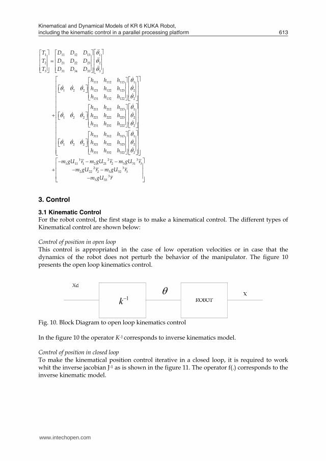
3. Control
3.1 Kinematic Control For the robot control, the first stage is to make a kinematical control. The different types of Kinematical control are shown below: Control of position in open loop This control is appropriated in the case of low operation velocities or in case that the dynamics of the robot does not perturb the behavior of the manipulator. The figure 10 presents the open loop kinematics control.
1k
Fig. 10. Block Diagram to open loop kinematics control In the figure 10 the operator K-1 corresponds to inverse kinematics model. Control of position in closed loop To make the kinematical position control iterative in a closed loop, it is required to work whit the inverse jacobian J-1 as is shown in the figure 11. The operator f(.) corresponds to the inverse kinematic model.
www.intechopen.com
Kinematical and Dynamical Models of KR 6 KUKA Robot, including the kinematic control in a parallel processing platform 613
Thus the vector h of centrifugal and Coriolis forces is:
,T
i i vh H
111 112 113 1
1 2 2 121 122 123 2
131 132 122 2
1 211 212 213 1
2 1 2 2 221 222 223 2
3 231 232 222 2
311 312 313
1 2 2 3
h h hh h hh h h
h h h hh h h hh h h h
h h hh
1
21 322 323 2
331 332 322 2
h hh h h
For the Determination of the gravity force vector C: 1 2 3( ) Tc c c c
3
1,2,3ji j ji j
j ic m gU r i
1 2 31 1 11 1 2 21 2 3 31 3c m gU r m gU r m gU r 2 3
2 2 22 2 3 32 3c m gU r m gU r 3
3 3 33 3c m gU r
1 2 31 1 11 1 2 21 2 3 31 3
2 32 2 22 2 3 32 3
33 3 33
c m gU r m gU r m gU rc m gU r m gU rc m gU r
The vector r in the reference system of rotation axes is:
1
1
0.00520.00260.369
1
r
2
2
00.2
0.3661
r
3
3
00.4540.00015
1
r
0 0 0g g The total system is then as follows:
( ) ( ( )) ( ) ( ( ), ( )) ( ( ))T t D t t h t t c t
1 11 12 13 1
2 21 22 23 2
3 31 34 33 3
111 112 113 1
1 2 2 121 122 123 2
131 132 122 2
211 212 213
1 2 2 221 222 223
231 232
T D D DT D D DT D D D
h h hh h hh h h
h h hh h hh h
1
2
222 2
311 312 313 1
1 2 2 321 322 323 2
331 332 322 2
1 2 31 11 1 2 21 2 3 31 3
2 32 22 2 3 32 3
3 3
h
h h hh h hh h h
m gU r m gU r m gU rm gU r m gU r
m gU
33 r
3. Control
3.1 Kinematic Control For the robot control, the first stage is to make a kinematical control. The different types of Kinematical control are shown below: Control of position in open loop This control is appropriated in the case of low operation velocities or in case that the dynamics of the robot does not perturb the behavior of the manipulator. The figure 10 presents the open loop kinematics control.
1k
Fig. 10. Block Diagram to open loop kinematics control In the figure 10 the operator K-1 corresponds to inverse kinematics model. Control of position in closed loop To make the kinematical position control iterative in a closed loop, it is required to work whit the inverse jacobian J-1 as is shown in the figure 11. The operator f(.) corresponds to the inverse kinematic model.
www.intechopen.com

Robot Manipulators, New Achievements614
Fig. 11. Iterative control position Joint Control Other option is to make a joint level control. In this case, the control is represented in the equation (19) in state variables.
( )
vJ
w (19)
Considering that most of the robots usually have a speed control loop at the level of joints: where for one input
du and a high-gain control k is found, the error tends to zero
0e and consequently u , the desired angular velocity. Figure 12.
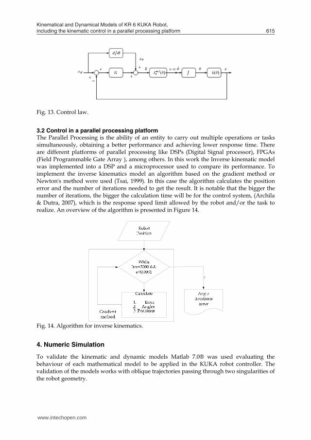
Fig. 12. Joint velocity control Therefore, the manipulator motion can be described by , 1,..., ,i iu i n were iu is a signal applied to the motor speed of the i-th joint. Then the control system to be considered is presented in the equation (20):
( )v
J uw
(20)
For the problem of trajectory tracking and to avoid errors in steady state, the control law u can be chosen as a proportional control adding one feed forward term. Equation (21) and figure 13 d du x K x x (21)
Fig. 13. Control law.
3.2 Control in a parallel processing platform The Parallel Processing is the ability of an entity to carry out multiple operations or tasks simultaneously, obtaining a better performance and achieving lower response time. There are different platforms of parallel processing like DSPs (Digital Signal processor), FPGAs (Field Programmable Gate Array ), among others. In this work the Inverse kinematic model was implemented into a DSP and a microprocessor used to compare its performance. To implement the inverse kinematics model an algorithm based on the gradient method or Newton's method were used (Tsai, 1999). In this case the algorithm calculates the position error and the number of iterations needed to get the result. It is notable that the bigger the number of iterations, the bigger the calculation time will be for the control system, (Archila & Dutra, 2007), which is the response speed limit allowed by the robot and/or the task to realize. An overview of the algorithm is presented in Figure 14.
‘'
Fig. 14. Algorithm for inverse kinematics.
4. Numeric Simulation
To validate the kinematic and dynamic models Matlab 7.0® was used evaluating the behaviour of each mathematical model to be applied in the KUKA robot controller. The validation of the models works with oblique trajectories passing through two singularities of the robot geometry.
www.intechopen.com
Kinematical and Dynamical Models of KR 6 KUKA Robot, including the kinematic control in a parallel processing platform 615
Fig. 11. Iterative control position Joint Control Other option is to make a joint level control. In this case, the control is represented in the equation (19) in state variables.
( )
vJ
w (19)
Considering that most of the robots usually have a speed control loop at the level of joints: where for one input
du and a high-gain control k is found, the error tends to zero
0e and consequently u , the desired angular velocity. Figure 12.
Fig. 12. Joint velocity control Therefore, the manipulator motion can be described by , 1,..., ,i iu i n were iu is a signal applied to the motor speed of the i-th joint. Then the control system to be considered is presented in the equation (20):
( )v
J uw
(20)
For the problem of trajectory tracking and to avoid errors in steady state, the control law u can be chosen as a proportional control adding one feed forward term. Equation (21) and figure 13 d du x K x x (21)
Fig. 13. Control law.
3.2 Control in a parallel processing platform The Parallel Processing is the ability of an entity to carry out multiple operations or tasks simultaneously, obtaining a better performance and achieving lower response time. There are different platforms of parallel processing like DSPs (Digital Signal processor), FPGAs (Field Programmable Gate Array ), among others. In this work the Inverse kinematic model was implemented into a DSP and a microprocessor used to compare its performance. To implement the inverse kinematics model an algorithm based on the gradient method or Newton's method were used (Tsai, 1999). In this case the algorithm calculates the position error and the number of iterations needed to get the result. It is notable that the bigger the number of iterations, the bigger the calculation time will be for the control system, (Archila & Dutra, 2007), which is the response speed limit allowed by the robot and/or the task to realize. An overview of the algorithm is presented in Figure 14.
‘'
Fig. 14. Algorithm for inverse kinematics.
4. Numeric Simulation
To validate the kinematic and dynamic models Matlab 7.0® was used evaluating the behaviour of each mathematical model to be applied in the KUKA robot controller. The validation of the models works with oblique trajectories passing through two singularities of the robot geometry.
www.intechopen.com

Robot Manipulators, New Achievements616
4.1 Computational model to validate the direct kinematics model In the validations of this model, the input data are angular positions for each joint and the positions for terminal elements are obtained, Figure 15. In this case the joint 2 and 3 takes angular increments up to a 90 degrees rotation in each link.
Fig. 15. Direct kinematic model.
4.2 Computational model to validate the inverse kinematics model The validation of this model requires knowledge of the spatial positions for the robot, the validation used an oblique path obtaining the following results Figure 16.
Fig. 16. Inverse kinematic model. Figure 16 shows that the inverse kinematics model follows the path requested, providing the angular positions needed to achieve the desired positions even for singular points in the workspace of the manipulator.
4.3 Computational model to validate the dynamical model To validate the dynamic model, the input data were oblique trajectories and tasks that require the motion of the terminal element with constant speed, working load of 16 kg
which corresponds to the maximum load recommended by KUKA Roboter (2005). Through the validated inverse kinematics algorithm the angular positions are calculated. Once obtained, the angular positions, it is calculated the angular velocities using the Jacobian inverse, obtaining the following joint speeds Figure 17.
Fig. 17. Angles and angular velocity for the joints. The angular accelerations required to perform the requested trajectory were calculated and the values are presented in Figure 18.
Fig. 18. Angular accelerations obtained in the joints. With the data of angular positions, angular velocities, angular accelerations and loads applied on the dynamic model of equation (14), the following values of the torques of the robot actuators are obtained, Figure 19.
www.intechopen.com

Kinematical and Dynamical Models of KR 6 KUKA Robot, including the kinematic control in a parallel processing platform 617
4.1 Computational model to validate the direct kinematics model In the validations of this model, the input data are angular positions for each joint and the positions for terminal elements are obtained, Figure 15. In this case the joint 2 and 3 takes angular increments up to a 90 degrees rotation in each link.
Fig. 15. Direct kinematic model.
4.2 Computational model to validate the inverse kinematics model The validation of this model requires knowledge of the spatial positions for the robot, the validation used an oblique path obtaining the following results Figure 16.
Fig. 16. Inverse kinematic model. Figure 16 shows that the inverse kinematics model follows the path requested, providing the angular positions needed to achieve the desired positions even for singular points in the workspace of the manipulator.
4.3 Computational model to validate the dynamical model To validate the dynamic model, the input data were oblique trajectories and tasks that require the motion of the terminal element with constant speed, working load of 16 kg
which corresponds to the maximum load recommended by KUKA Roboter (2005). Through the validated inverse kinematics algorithm the angular positions are calculated. Once obtained, the angular positions, it is calculated the angular velocities using the Jacobian inverse, obtaining the following joint speeds Figure 17.
Fig. 17. Angles and angular velocity for the joints. The angular accelerations required to perform the requested trajectory were calculated and the values are presented in Figure 18.
Fig. 18. Angular accelerations obtained in the joints. With the data of angular positions, angular velocities, angular accelerations and loads applied on the dynamic model of equation (14), the following values of the torques of the robot actuators are obtained, Figure 19.
www.intechopen.com

Robot Manipulators, New Achievements618
Fig. 19. Torques obtained in the joints. The data provided by KUKA Roboter (2005) are presented in Table 4, It shows the operational limits of the robot.
KUKA KR 6 Maximum Torque 3400 Nm Total mass 206 Kg + 16 Kg Maximum Velocity 600 Degrees/sec Repeatability +/- 0,1 mm
Table 4. Technical data to KR6 KUKA Robot
4.4 Implementation in a parallel processing platform The inverse kinematics algorithm was implemented in VisualDSP®, Matlab® and C® to observe its performance, evaluating the processing time and the position error. Processing Time To evaluate the processing time, oblique trajectories were used in the same way as in the case of the dynamic model validation. The processing times obtained are presented in Figure 20 which clearly shows that the DSP has the shortest processing time.
Fig. 20. Comparation of processing time
Evaluation of processing time The Figure 20 shows that the DSP processing time is the shortest. However, we must assess whether it is appropriate to implement it as a Possible driver. For this purpose it is necessary to review the technical data of the robot to know its response speed. This data can be seen in Table 5, where the main information are: the encoder pulses and maximum angular velocity to which the robot can move, due to technical characteristics of the servo motors used to its operation.
Encoder 512 Pulses/Rev 1,422 Pulses/Degree
W Max 600 Degrees/sec Frequency 853,33 Pulses/sec
Period 0,00117 sec/pulse 0,703 Degrees/pulse 0,0123 Radians/pulse
Table 5. Technical data to calculus of response speed of KR6 KUKA Robot The Figure 21 shows that the DSP processing time is appropriated to be implemented as a controller because it offers a maximum response of 0.55 ms, and the robot required 1.17 ms.
Fig. 21. DSP Processing time Position Error Another important characteristic to evaluate, is the position error which corresponds to two main factors: the first one is the quantization error and the second one the error due to the calculation method. The Figure 25 shows the position errors. The comparison parameter corresponds to the repeatability of the robot, which for this case is 0.1 mm in accordance to Figure 22.
Fig. 22. Position error In the figure 22, the maximum position error of the DSP is 0.08 mm.
www.intechopen.com

Kinematical and Dynamical Models of KR 6 KUKA Robot, including the kinematic control in a parallel processing platform 619
Fig. 19. Torques obtained in the joints. The data provided by KUKA Roboter (2005) are presented in Table 4, It shows the operational limits of the robot.
KUKA KR 6 Maximum Torque 3400 Nm Total mass 206 Kg + 16 Kg Maximum Velocity 600 Degrees/sec Repeatability +/- 0,1 mm
Table 4. Technical data to KR6 KUKA Robot
4.4 Implementation in a parallel processing platform The inverse kinematics algorithm was implemented in VisualDSP®, Matlab® and C® to observe its performance, evaluating the processing time and the position error. Processing Time To evaluate the processing time, oblique trajectories were used in the same way as in the case of the dynamic model validation. The processing times obtained are presented in Figure 20 which clearly shows that the DSP has the shortest processing time.
Fig. 20. Comparation of processing time
Evaluation of processing time The Figure 20 shows that the DSP processing time is the shortest. However, we must assess whether it is appropriate to implement it as a Possible driver. For this purpose it is necessary to review the technical data of the robot to know its response speed. This data can be seen in Table 5, where the main information are: the encoder pulses and maximum angular velocity to which the robot can move, due to technical characteristics of the servo motors used to its operation.
Encoder 512 Pulses/Rev 1,422 Pulses/Degree
W Max 600 Degrees/sec Frequency 853,33 Pulses/sec
Period 0,00117 sec/pulse 0,703 Degrees/pulse 0,0123 Radians/pulse
Table 5. Technical data to calculus of response speed of KR6 KUKA Robot The Figure 21 shows that the DSP processing time is appropriated to be implemented as a controller because it offers a maximum response of 0.55 ms, and the robot required 1.17 ms.
Fig. 21. DSP Processing time Position Error Another important characteristic to evaluate, is the position error which corresponds to two main factors: the first one is the quantization error and the second one the error due to the calculation method. The Figure 25 shows the position errors. The comparison parameter corresponds to the repeatability of the robot, which for this case is 0.1 mm in accordance to Figure 22.
Fig. 22. Position error In the figure 22, the maximum position error of the DSP is 0.08 mm.
www.intechopen.com

Robot Manipulators, New Achievements620
5. Conclusions
The work presents the direct kinematics model of the robot KUKA KR 6, which was evaluated, obtaining suitable results for the kinematic control implemented. The inverse kinematics model using the quadratic equation was shown to be an appropriated method. It presents the possible configurations of the robot in order to achieve the desired position to follow a trajectory. The calculation of the inertia tensor was performed with the aid of CAD software, which gives us the principal inertia moments, products of inertia, and the centroid location of each link of the robot Is Important to show that the inertia tensor obtained needs to be understood and translated to the appropriate reference system for the dynamic model. The dynamic model was evaluated, obtaining values of 1250 Nm of torque to the oblique trajectory at constant speed work-rate. Obtaining as a maximum speed 12.7 RPM in the joint two, working well within the parameters of the KUKA Roboter. The performance evaluation of the DSP was adequate, obtaining a processing time of 0.55 ms, appropriate for the given operation. The position error found corresponds to the calculation method and the quantization error The maximum error value found was 0.08 mm which is below the repeatability value given by KUKA Roboter.
6. References
Archila J. F, Dutra M. S., (2007). Design and construction of a SCARA Type Manipulator, implementing a control system, International Congress of Mechanical Engineering COBEM 2007. Brasilia.
Barrientos, A., (2001). Fundamentos de robótica, McGraw Hill, pp 15 – 38 Beer F., (1980) Mecânica Vetorial para Engenheiros, McGraw H, pp 399 – 447. Denavit, J., Hartenberg R. S., (1955) A Kinematic Notation for Lower- Pair Mechanism Based
on Matrices, Journal of Applied Mechanics 22: 215 –221. Dutra, M. S., (2006). Notas de Aula Mecanismos, Universidade Federal do Rio de Janeiro
UFRJ. Fu K. S., (1987) Control, Sensing, Vision, and Intelligence, McGraw Hill, pp 82 – 102. KUKA Roboter. (2005)Technical specifications Manual. Kurfles, T., (2005). Robotics and Automation Handbook. CRC Press, pp 26 - 84 Ollero, A., (2001). Robótica, Manipuladores y robots móviles, Primera edición, Alfaomega,
Barcelona, pp 43 - 80 Tsai L. W., (1999) Robot Analysis. The Mechanics of Serial and Parallel Manipulators.
Editorial John Wiley & Sons, Inc, pp 55 – 72. Visual DSP ++ 4.5, C/C++ Compiler and library Manual for sharc, Analog Device.
www.intechopen.com
Robot Manipulators New AchievementsEdited by Aleksandar Lazinica and Hiroyuki Kawai
ISBN 978-953-307-090-2Hard cover, 718 pagesPublisher InTechPublished online 01, April, 2010Published in print edition April, 2010
InTech EuropeUniversity Campus STeP Ri Slavka Krautzeka 83/A 51000 Rijeka, Croatia Phone: +385 (51) 770 447 Fax: +385 (51) 686 166www.intechopen.com
InTech ChinaUnit 405, Office Block, Hotel Equatorial Shanghai No.65, Yan An Road (West), Shanghai, 200040, China
Phone: +86-21-62489820 Fax: +86-21-62489821
Robot manipulators are developing more in the direction of industrial robots than of human workers. Recently,the applications of robot manipulators are spreading their focus, for example Da Vinci as a medical robot,ASIMO as a humanoid robot and so on. There are many research topics within the field of robot manipulators,e.g. motion planning, cooperation with a human, and fusion with external sensors like vision, haptic and force,etc. Moreover, these include both technical problems in the industry and theoretical problems in the academicfields. This book is a collection of papers presenting the latest research issues from around the world.
How to referenceIn order to correctly reference this scholarly work, feel free to copy and paste the following:
John Faber Archila Diaz, Max Suell Dutra and Fernando Augusto de Noronha Castro Pinto (2010). Kinematicaland Dynamical Models of KR 6 KUKA Robot, Including the Kinematic Control in a Parallel Processing Platform,Robot Manipulators New Achievements, Aleksandar Lazinica and Hiroyuki Kawai (Ed.), ISBN: 978-953-307-090-2, InTech, Available from: http://www.intechopen.com/books/robot-manipulators-new-achievements/kinematical-and-dynamical-models-of-kr-6-kuka-robot-including-the-kinematic-control-in-a-parallel-pr