3.3 pollution load analysis

Chapter 3 - Pollution Analysis

3 - 16

3.3 POLLUTION LOAD ANALYSIS

3.3.1 METHODOLOGY

The basic purpose of pollution load analysis is to estimate pollution load reaching the bay through each river basin and to estimate the contribution of pollution sources. Estimated pollution load has been used as input data for the water quality simulation model as well as base information for the estimation of pollution loads in the future. Estimates are made for the years 2000, 2010 and 2020 based on population estimates of the year in question. Further load estimates has been made assuming an increasing part of the population being served by at treatment plant. The load estimates has all been used for simulations of the water quality in the bay. Figure 3.8 shows the schematic diagram of pollution load estimation.

(1) Category of Pollution Sources

Pollution sources are categorized into point and non-point sources. Point sources can be defined as known loads for which the location of discharge is known. WWTP discharge and large industry discharge are point sources. All other sources are categorized as non-point sources which include the areal pollution load originating from urban, agricultural and natural processes.

(2) Estimation of Pollution Load

Pollution loads are estimated for the following.

Point sources

- Generation of pollution load by population - Pollution load discharge by WWTP and large industries - Pollution load discharged by small-scale treatment units for shopping centers, hospitals,

schools etc.

Non-Point sources

- Areal pollutant load reaching the river due to natural, agricultural and urban origin (3) Pollution Load Reaching the Bay through Rivers

Based on the monitored river water quality and estimated river flow, monitored pollution load (LMON) to the bay through each river basin is estimated to compare the pollution load generated and pollution load discharged to the bay utilizing water quality monitoring data and estimated basin discharge.

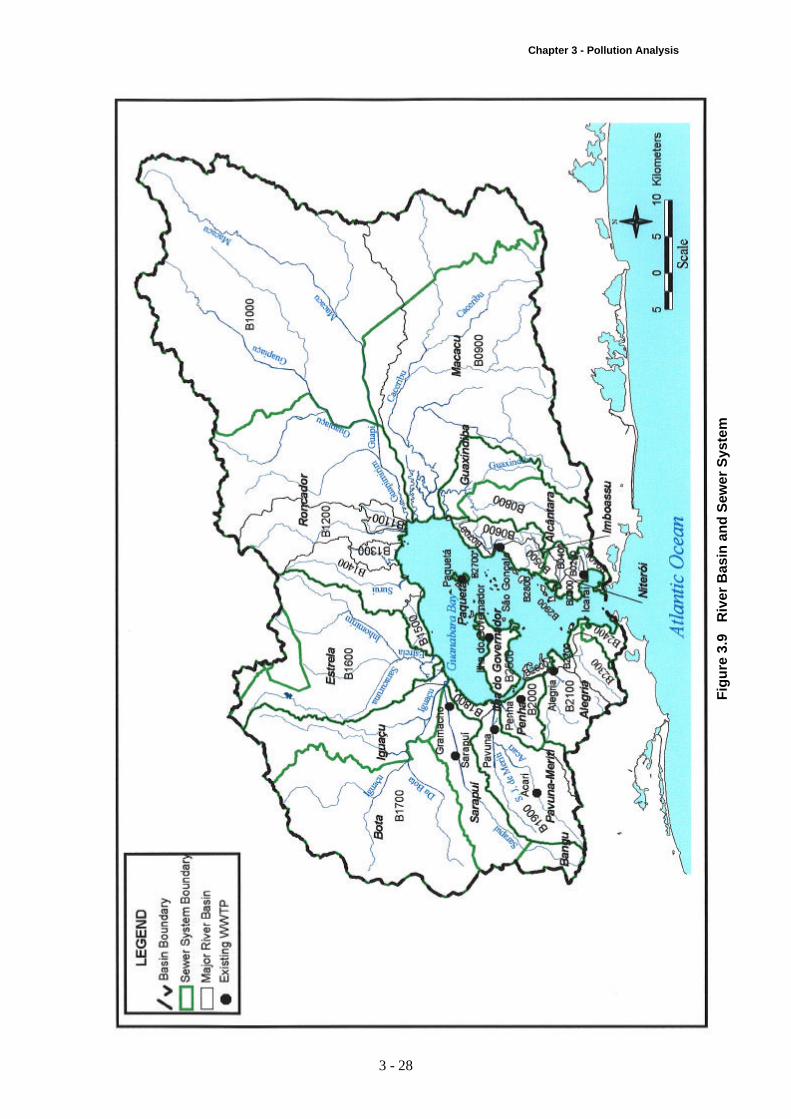
3.3.2 RIVER BASIN AND SEWER SYSTEM

Figure 3.9 shows boundaries of river basins and sewer systems. Sewer system boundary of CEDAE Sewer Master Plan is reviewed. Existing WWTP locations are also shown in the figure.

3.3.3 POLLUTION LOAD GENERATED BY HUMAN WASTE

Population connected to the WWTP (referred to as Sewage Treatment Population) is estimated based on the sewer service ratio and the incoming flow to WWTP. The below listed per capita pollution load generation for BOD, total N, total P and E. coli bacteria is used:

BOD: 54 g BOD/day, TN: 10 g N/day, TP: 2.5 g P/day E. coli: 109/day

Pollution load generated (LPOP-without sewer) is calculated based on the unit per capita generation and population which is not connected to the sewerage for each river basin.


3 - 17

Table 3.4 shows the population by river basin based on the year 2000 census. Table 3.5 shows estimate of BOD5 load generation by total population classifyied into population connected to WWTP and population not connected to WWTP. Total BOD5 load generated is 445 ton/day out of which (75 %) of the pollution load generated is not treated at WWTP.

3.3.4 POLLUTION LOAD AT WWTP

Pollution load discharged through WWTP (LWWTP-Dis) is obtained considering efficiency of WWTP. As shown in Table 3.6, total BOD5 load to WWTP is 110 ton/day out of which 73 ton/day is removed resulting in 37 ton/day discharged to “waterbody” of rivers or directly to the Bay. Six of the listed WWTP discharge to the Bay. These are: Icarai, San Goncalo, Penha, Alegria, I. Do Governado, I. Do Paqueta.

3.3.5 POLLUTION LOAD DISCHARGED BY INDUSTRIES

FEEMA is carrying out an action program to control the pollution load from industries and has established a database of industrial pollution load of major polluters and implementing a program to reduce pollution load of industries. Under these program, 455 industries are selected. Out of these, 55 industries are classified as Priority 1 industries, which discharge 80% of the pollution load. A database of pollution load discharged by the major polluting industries which consists of 155 industries including Priority 1 and Priority 2 industries was completed by FEEMA through self-reporting of industries and the data was obtained by the Study Team. Total BOD pollution load of these 155 industries in year 2000 is estimated to be 9.64 ton/day. Number of industries not covered under the above are small and medium scale industries but are large in number. Pollution load of these industries is approximately 12 ton/day.

Data on nutrient load from industries have not been available, therefore ratios for TN/BOD and TP/BOD of 0.44 g N/g BOD and 0.079 g P/g BOD has been used to estimate the industrial total N and total P load (Diego-Mclone et al, 2000)

3.3.6 OTHER POINT SOURCES (SMALL- SCALE TREATMENT UNITS) Small-scale treatment units for developments such as condominium, hospitals, shopping centers, schools etc. has been registered with FEEMA under the “non-industry” category and data is obtained for 69 such units, on their location and pollution load.

Distribution of total industrial and non-industrial pollution load by river basin is shown in Table 3.7.

3.3.7 AREAL POLLUTION LOAD

Areal pollution load due to natural, agricultural or urban sources can be estimated for a known section of basin if monitoring data is available at the inlet and outlet of the river through the basin and the point source pollution load is known. Only one such location is available in the Macacu River at FEEMA Monitoring location MC-967 which coincides with SERLA river gauging station 18. At this location, which is the uppermost sub-basin where point sources are negligible, pollution load is due to natural origin for which a reasonable number of flow and water quality measurements are available for the year 1994, year 1999 and year 2000. Relationship between specific BOD load (LBOD) and specific discharge (Qs) is obtained thorough regression (Figure 3.10) as follows:


3 - 18

LBOD=0.268Qs0.824

Where, LBOD is in kg/(km2⋅d) and Qs is in L/(km2⋅s).

Figure 3.10 Relationship between Specific Load and Specific Discharge at MC967

Relationship between specific TN load (LTN), TP load (LTP), PO4-P load (LPO4), DIN load (LDIN) and specific discharge (Qs) is obtained thorough regression as follows:

LTN=0.072Qs0.9142

LTP=0.0032Qs1..3016

LPO4=0.00286Qs0.9905

LDIN=0.0821Qs0.6201

In the absence of monitored data, the above relationships have been utilized to estimate the real pollution load though they don’t include the load during extreme rainfall events.

3.3.8 RUN OFF RATIO OF GENERATED POLLUTION LOAD

Monitored pollution load (LMON) is calculated for river basins utilizing water quality monitoring data where available and estimated basin discharge. There were six measurements of water quality in year 2000 and monitoring of water quality is generally not during storms. To include the load due to rain, it is assumed that the water quality of the river remains constant throughout the year and is obtained from the average of monitored quality. For those stations without water quality monitoring station, approximate estimation is made based on either population density or area depending on the type of basin. Estimated discharge load to the bay for year 2000 is 252 ton/day.

For each of the river basin, run-off ratio is calculated. Run-off ratio is calculated as total pollution load (LRIVER) discharged to the rivers (as shown in Table 3.7) which is the sum of pollution load discharged through WWTP (LWWTP-Dis), pollution load generated by large industries (LI), small-scale treatment units (LNI), and areal pollution load (LAREAL) to the monitored pollution load (LMON).

Spec i f c Load Vs Spec i f i c D i scha r ge a t MC967

y = 0.824 x - 1.317

-0.5

0.0

0.5

1.0

1.5

2.0

2.5

3.0

3.5

0 1 2 3 4 5

Ln(specific discharge)

Ln(s

pecific

BO

D L

oad

)

LBOD=0.268Qs0.824


3 - 19

LRIVER = LWWTP-Dis + LPOP-without sewer + LI + LNI + LAREAL

Run-off Ratio = LMON / LRIVER

Preliminary estimate of the run-off ratio is 0.67 for the whole of the basin of Guanabara Bay assuming that all of the pollution load generated by the population not treated by the WWTP reaches the bay.

When comparing the monitored load with the generated load basin by basin a great variation in the Run-off ratio can be observed. In some cases the monitored load is higher than the generated load, a great deal of this variation can be related to lack of frequent and consistent measurements of both concentrations and discharge on the same location in the river.

It has therefore decided to estimate the run-off ratio for each major basin based on assumed degradation rates for of BOD, TN, TP and E. coli and an estimated the average retention for the water each basin. The mineralization of BOD, the death of E. Coli, denitrification and other immobilization of TN and immobilization of TP is described by the below equation exemplified by BOD:

L=BOD*eK*t

Where K is the daily mineralization rate (1/d) and t is the average time for pollutants in a specific basin to flow from the source to the Bay. The average retention time is estimated from the distance of the pollution centers in term of cities or industrial areas to the Bay and a velocity of the water in the river. The average velocity of the water is set to 0.05 m/sec. K values for different components are set to:

BOD: K=0.3 1/d, TN: K=0.2 1/d, TP: K=0.1 1/d E. coli: K=0.8 1/d

Please refer to Supporting 5 on Pollution Load Analysis for run-off ratios by river basin .

3.3.9 POLLUTION LOAD DISCHARGED TO BAY

The total BOD load reaching the Bay through rivers after self-purification and directly from WWTP discharging to the Bay is presented in the Table 3.8. Please refer to Supporting 5 on Pollution Load Analysis for total N, P and E. coli load reaching the bay after self-purification.

In year 2000, the load to the bay is estimated to be 275 ton BOD/day, 72 ton TN/day, 18.4 ton TP/day and 3.07×1015 E. coli bacteria per day.

3.3.10 POPULATION IN YEAR 2010 AND 2020

To be able to predict the load to the Bay in the future, the population size has to be predicted for the future. In the present study, year 2010 and year 2020 has been chosen as future reference years. The average annual growth ratio (AAGR) until year 2020 for the whole basin has been estimated to be 0.67 %. The annual growth ratios however vary over time and with administrative areas and thereby also with basins.

Total population in the Bay catchment was 8,290,300 in year 2000. The projections of the population size for 2010 and 2020 by river basin are presented in Table 3.4. The population size is expected to increases to 9,013,026 in year 2010 and 9,619,561 in year 2020.


3 - 20

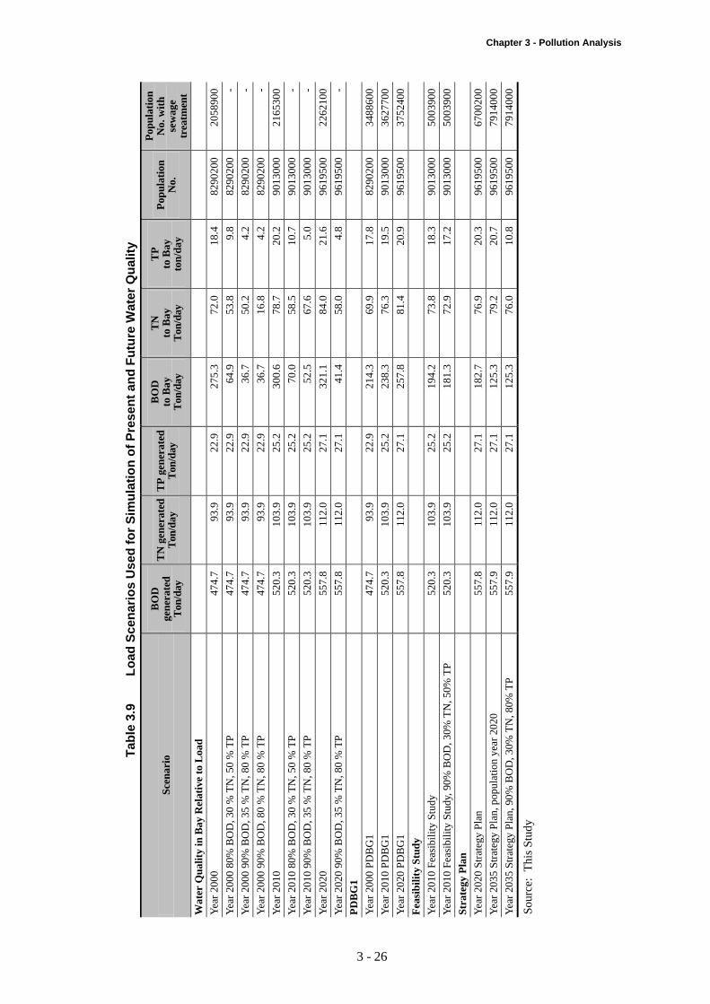
3.3.11 FUTURE LOAD AND LOAD SCENARIOS

The load of BOD and nutrients has been estimated to be able to predict the future water quality in the Bay with the eutrophication model.

A series of simulations has been conducted with the purpose of estimating the load at which standards of 10 mg BOD/l and 5 mg BOD/l are achieved in the Bay. The series include simulations of year 2000, year 2010 and year 2020 populations and industrial development. In Table 3.9, the scenarios are presented under title “Water Quality in Bay Relative to Load”. The table includes columns with data for generated load, load to Bay, population and population with sewage treatment. Three set of reduced domestic and industrial loads are included in this series: one with 80 % BOD, 30 % TN and 50 % TP reduction of domestic and industrial load after existing treatment but before self purification in rivers; one with 90 % BOD, 35 % TN and 80 % TP reduction; and one with 90% BOD, 80% TN and 80% TP load reduction. The small natural background load is the same for all scenarios.

A second series of simulations (under title “PDBG1” in Table 3.9) has been conducted predicting the water quality in the Bay implementing treatment according to the PDBG1 plan for populations and industrial load of year 2000, year 2010 and year 2020. The population with sewage treatment is assumed to increase with the increase in population within existing areas connected to a treatment plant.

A third series of simulations (under title “Feasibility Study” in Table 3.9) has been conducted estimating the water quality in year 2010 using a Feasibility Plan with about 55 % of the population connected to a treatment plant. One scenario is labeled “Year 2010 Feasibility Study” assuming secondary treatment removing 90 % BOD, 25 % TN and 20 % TP for all plants except for 3 plants (Icarai, Sarapuí & Puvuna) which all have primary treatment with chemical precipitation giving a reduction of 55% BOD, 35 % TN and 80 % TP. And the other scenario is where all treatment plants have secondary treatment with chemical precipitation reducing the load with 90 % for BOD, 30 % for TN and 50 % for TP.

And fourth series of load scenarios (under title “Strategy Plan” in Table 3.9) has been prepared according to the Strategy Plan for year 2020 and for year 2035 using population size of year 2020. Scenario for year 2020 assumes all treatment plants have secondary treatment except Icarai, Sarapuí and Puvuna, which has primary treatment with precipitation. Scenario for year 2035 assumes all treatment plants having secondary treatment but the population size is from year 2020. The last scenario for year 2035 assumes all treatment plants having 90% BOD, 30% TN and 50% TP removal.

References for section 3.3 Maria Louredes San Diego-Mclone, Stephen V. Smith, Vivian F. Nicolas. Stoichiometric Interpretations of C:N:P ratios in organic waste materials. Marine Pollution Bulletin Vol. No. 4 pp 325-330, 2000.


3 - 21

Table 3.4 Population in the Basin for Year 2000, 2010 and 2020

Region No. Basin Name Basin Area (km2)

Population (year 2000)



Sewage Treatment Population (year 2000)

Population without Sewage

Treatment (year 2000)

E B0100 B. Charitas 9.46 30,559 31,989 33,686 13,752 16,807 E B0200 Canal Canto do Rio 6.21 90,467 94,702 99,725 40,710 49,757 E B0300 B. Catedrar 7.57 91,390 95,668 100,742 41,126 50,264 E B0400 B. Norte Centro 9.26 71,373 74,704 78,666 32,118 39,255 E B0500 Rio Bomba 26.78 241,500 269,240 294,737 54,491 187,009 E B0600 Rio Imboassu 29.43 157,098 178,840 198,168 19,987 137,111

NE B0700 B. Itaoca 8.54 2,578 2,935 3,252 328 2,250 NE B0800 Rio Alcântara 173.07 593,400 676,100 748,144 - 593,400 NE B0900 Rio Cacerebú 811.34 256,254 311,969 353,046 - 256,254 NE B1000 Rio Guapimirim 1,262.03 87,059 104,593 122,045 - 87,059 NE B1100 Canal de Magé 17.08 33,734 43,009 49,309 - 33,734 NE B1200 Rio Roncador 115.19 30,316 38,641 44,271 - 30,316 NE B1300 Rio Iriri 19.63 4,659 5,938 6,800 - 4,659 NE B1400 Rio Surui 84.44 22,169 28,253 32,354 - 22,169 NW B1500 B. Maua 17.92 13,450 17,141 19,629 - 13,450 NW B1600 Rio Estrela 348.88 385,215 451,791 508,699 - 385,215 NW B1700 Rio Iguaçú 716.72 1,024,170 2,452,033 2,647,683 - 1,024,170 W B1707 Rio Sarapuí 1,172,773 476,450 696,323 W B1800 B. Cabo do Brito 19.72 54,430 62,559 70,699 21,772 32,658 W B1900 Rio S. J. Meriti 154.26 1,397,082 1,453,394 1,506,410 415,833 981,249 W B2000 Rio Irajá 50.95 682,128 706,115 728,215 544,770 137,358 W B2100 Canal do Cunha 70.23 899,762 931,393 960,535 147,500 752,262 W B2200 B. São Cristóvão 6.41 30,459 31,530 32,516 5,269 25,190 W B2300 Canal do Mangue 37.95 440,731 456,225 470,500 73,454 367,277 W B2400 B. Botafogo 21.68 262,642 271,875 280,382 8,970 253,672 I B2500 I. do Governador 36.28 209,426 216,788 223,571 159,164 50,262 I B2600 I. do Fundão 5.35 1,826 1,890 1,949 1,826 I B2700 I. de Paquetá 2.21 3,586 3,712 3,828 3,227 359 I B2800 I. do Engenho 0.98 - 0 0 - I B2900 I.de S. Cruz 1.10 - 0 0 -

Total 4,070.7 8,290,200 9,013,026 9,619,561 2,058,900 6,231,300

Source: This Study


3 - 22

Table 3.5 BOD Load Generation in the Basin for Year 2000

Region No. Basin Name Basin Area

(km2)

Total BOD5 Load Generated

(ton/d)

BOD5 Load to WWTP within Sewer System

Area (ton/d)

BOD5 Load Generated by Population

without Sewage Treatment

E B0100 B. Charitas 9.46 1.7 0.7 0.9 E B0200 Canal Canto do Rio 6.21 4.9 2.2 2.7 E B0300 B. Catedrar 7.57 4.9 2.2 2.7 E B0400 B. Norte Centro 9.26 3.9 1.7 2.1 E B0500 Rio Bomba 26.78 13.0 2.9 10.1 E B0600 Rio Imboassu 29.43 8.5 1.1 7.4

NE B0700 B. Itaoca 8.54 0.1 0.0 0.1 NE B0800 Rio Alcântara 173.07 32.0 - 32.0 NE B0900 Rio Cacerebú 811.34 13.8 - 13.8 NE B1000 Rio Guapimirim 1,262.03 4.7 - 4.7 NE B1100 Canal de Magé 17.08 1.8 - 1.8 NE B1200 Rio Roncador 115.19 1.6 - 1.6 NE B1300 Rio Iriri 19.63 0.3 - 0.3 NE B1400 Rio Surui 84.44 1.2 - 1.2 NW B1500 B. Maua 17.92 0.7 - 0.7 NW B1600 Rio Estrela 348.88 20.8 - 20.8 NW B1700 Rio Iguaçú 716.72 55.3 - 55.3 W B1707 Rio Sarapuí 63.3 25.7 37.6 W B1800 B. Cabo do Brito 19.72 2.9 1.2 1.8 W B1900 Rio S. J. Meriti 154.26 75.4 22.5 53.0 W B2000 Rio Irajá 50.95 36.8 29.4 7.4 W B2100 Canal do Cunha 70.23 48.6 8.0 40.6 W B2200 B. São Cristóvão 6.41 1.6 0.3 1.4 W B2300 Canal do Mangue 37.95 23.8 4.0 19.8 W B2400 B. Botafogo 21.68 14.2 0.5 13.7 I B2500 I. do Governador 36.28 11.3 8.6 2.7 I B2600 I. do Fundão 5.35 0.1 - 0.1 I B2700 I. de Paquetá 2.21 0.2 0.2 0.0 I B2800 I. do Engenho 0.98 - - - I B2900 I.de S. Cruz 1.10 - - - Total 4,070.7 447.7 111.2 336.5 Per capita BOD generation 54 g/(capita⋅d)

Source: This Study


3 - 23

Table 3.6 BOD Load at WWTP for Year 2000

Region No. Basin Name Basin Area (km2)

Name of WWTP

Load to WWTP (ton/d)

Load Removed at WWTP

(ton/d)

WWTP Load Discharged to Water Body

(ton/d)

E B0100 B. Charitas 9.46

E B0200 Canal Canto do Rio 6.21 Icarai 8.913 4.902 4.011 E B0300 B. Catedrar 7.57 E B0400 B. Norte Centro 9.26

E B0500 Rio Bomba 26.78 San Goncalo 2.018 1.816 0.202 E B0600 Rio Imboassu 29.43

NE B0700 B. Itaoca 8.54 NE B0800 Rio Alcântara 173.07

NE B0900 Rio Cacerebú 811.34 NE B1000 Rio Guapimirim 1,262.03 NE B1100 Canal de Magé 17.08 NE B1200 Rio Roncador 115.19

NE B1300 Rio Iriri 19.63 NE B1400 Rio Surui 84.44 NW B1500 B. Maua 17.92 NW B1600 Rio Estrela 348.88

NW B1700 Rio Iguaçú 716.72 Sarapuí Gramacho

25.728 14.311 11.427

NW B1800 B. Cabo do Brito 19.72 W B1900 Rio S. J. Meriti 154.26 Pavuna

Acarai 22.455 13.806 8.649

W B2000 Rio Irajá 50.95 Penha 29.418 26.476 2.942 W B2100 Canal do Cunha 70.23 Alegria 12.700 3.810 8.890

W B2200 B. São Cristóvão 6.41 W B2300 Canal do Mangue 37.95 W B2400 B. Botafogo 21.68 I B2500 I. do Governador 36.28 I. do

Governador 8.595 7.735 0.859

I B2600 I. do Fundão 5.35 I B2700 I. de Paquetá 2.21 I. de Paquetá 0.174 0.141 0.017 I B2800 I. do Engenho 0.98

I B2900 I.de S. Cruz 1.10

Total 4,070.7 110.10 73.01 36.99

Source: This Study


3 - 24

Table 3.7 Summary of Total BOD Load for Year 2000

Region No. Basin Name Basin Area

(km2)

WWTP Load

(ton/d)

Untreated Domestic Load

(ton/d)

Industrial/Non-industrial Load

(ton/d)

Surface Pollution Load

(ton/d)

E B0100 B. Charitas 9.46 - 0.91 0.735 0.011 E B0200 Canal Canto do Rio 6.21 4.01 2.69 0.033 0.007 E B0300 B. Catedrar 7.57 - 2.71 - 0.009

E B0400 B. Norte Centro 9.26 - 2.12 - 0.010 E B0500 Rio Bomba 26.78 0.20 10.1 4.108 0.032 E B0600 Rio Imboassu 29.43 - 7.40 - 0.033

NE B0700 B. Itaoca 8.54 - 0.12 - 0.010

NE B0800 Rio Alcântara 173.07 - 32.04 0.997 0.180 NE B0900 Rio Cacerebú 811.34 - 13.84 0.183 0.722 NE B1000 Rio Guapimirim 1,262.03 - 4.70 1.308 0.003 NE B1100 Canal de Magé 17.08 - 1.82 0.000 0.022

NE B1200 Rio Roncador 115.19 - 1.64 0.054 0.240 NE B1300 Rio Iriri 19.63 - 0.25 - 0.022 NE B1400 Rio Surui 84.44 - 1.20 0.051 0.118 NW B1500 B. Maua 17.92 - 0.73 - 0.020

NW B1600 Rio Estrela 348.88 - 20.80 2.398 0.674 NW B1700 Rio Iguaçú 716.72 11.42 55.31 2.666 1.003 W B1707 Rio Sarapuí 37.60 3.051 W B1800 B. Cabo do Brito 19.72 - 1.76 0.218 0.029

W B1900 Rio S. J. Meriti 154.26 8.65 52.99 1.826 0.217 W B2000 Rio Irajá 50.95 2.94 7.42 0.900 0.075 W B2100 Canal do Cunha 70.23 8.89 40.62 3.049 0.108 W B2200 B. São Cristóvão 6.41 - 1.26 0.245 0.010

W B2300 Canal do Mangue 37.95 - 19.83 0.425 0.054 W B2400 B. Botafogo 21.68 - 13.7 0.898 0.027 I B2500 I. do Governador 36.28 0.86 2.71 0.097 0.052 I B2600 I. do Fundão 5.35 - 0.1 - 0.008

I B2700 I. de Paquetá 2.21 0.02 0.02 - I B2800 I. do Engenho 0.98 - - - I B2900 I.de S. Cruz 1.10 - - -

Total 4,070.7 36.99 336.5 23.2 3.8

Source: This Study


3 - 25

Table 3.8 Total Load of BOD in ton/day Reaching Guanabara Bay After Self-purification in the Basins, Year 2000

No. Basin Name BOD Produced

BOD to bay

WWTP direct

Back ground Total

100 B. Charitas 1.6 1.5 0.011 1.5

200 Canal Canto do Rio 2.7 2.5 4.01 0.007 6.5

300 B. Catedrar 2.7 2.5 0.009 2.6

400 B. Norte Centro 2.1 1.7 0.010 1.8

500 Rio Bomba 14.2 12.4 0.20 0.032 12.7

600 Rio Imboassu 7.4 5.8 0.033 5.9

700 B. Itaoca 0.1 0.1 0.010 0.2

800 Rio Alcântara 33.0 16.5 0.180 17.2

900 Rio Cacerebú 14.0 4.9 0.722 5.8

1000 Rio Guapimirim 6.0 0.7 0.003 7.0

1100 Canal de Magé 1.8 1.5 0.022 1.6

1200 Rio Roncador 1.7 1.0 0.240 1.5

1300 Rio Iriri 0.3 0.2 0.022 0.3

1400 Rio Surui 1.2 0.9 0.118 1.3

1500 B. Maua 0.7 0.7 0.020 0.8

1600 Rio Estrela 23.2 16.4 0.674 18.6

1700 Rio Iguaçú 58.0 35.7 1.003 35.8

1707 Rio Sarapuí 52.1 32.0 32.0

1800 B. Cabo do Brito 2.0 1.8 0.029 2.0

1900 Rio S. J. Meriti 57.8 40.8 0.217 42.3

2000 Rio Irajá 8.3 5.9 2.94 0.075 9.2

2100 Canal do Cunha 43.7 35.5 8.89 0.108 44.8

2200 B. São Cristóvão 1.6 1.5 0.010 1.5

2300 Canal do Mangue 20.3 17.6 0.054 17.9

2400 B. Botafogo 14.6 13.6 0.027 13.8

2500 I. do Governador 2.8 2.8 0.86 0.052 3.7

2600 I. do Fundão 0.1 0.1 0.008 0.1

2700 I. de Paquetá 0.0 0.0 0.02 0.0

2800 I. do Engenho 0.0 0.0 0.0

2900 I.de S. Cruz 0.0 0.0 0.0

Total 374.1 256.7 16.9 3.8 275.2

Note: The “BOD produced” is the sum treated and untreated load from population and industry discharged to rivers in the basin.

Source: This Study


3 - 26

Tab

le 3

.9

Lo

ad S

cen

ario

s U

sed

fo

r S

imu

lati

on

of

Pre

sen

t an

d F

utu

re W

ater

Qu

alit

y

Scen

ario

B

OD

ge

nera

ted

Ton

/day

TN

gen

erat

ed

Ton

/day

T

P g

ener

ated

T

on/d

ay

BO

D

to B

ay

Ton

/day

TN

to

Bay

T

on/d

ay

TP

to

Bay

to

n/da

y

Pop

ulat

ion

No.

Pop

ulat

ion

No.

wit

h se

wag

e tr

eatm

ent

Wat

er Q

ualit

y in

Bay

Rel

ativ

e to

Loa

d

Yea

r 20

00

474.

7 93

.9

22.9

27

5.3

72.0

18

.4

8290

200

2058

900

Yea

r 20

00 8

0% B

OD

, 30

% T

N, 5

0 %

TP

47

4.7

93.9

22

.9

64.9

53

.8

9.8

8290

200

-

Yea

r 20

00 9

0% B

OD

, 35

% T

N, 8

0 %

TP

47

4.7

93.9

22

.9

36.7

50

.2

4.2

8290

200

-

Yea

r 20

00 9

0% B

OD

, 80

% T

N, 8

0 %

TP

47

4.7

93.9

22

.9

36.7

16

.8

4.2

8290

200

-

Yea

r 20

10

520.

3 10

3.9

25.2

30

0.6

78.7

20

.2

9013

000

2165

300

Yea

r 20

10 8

0% B

OD

, 30

% T

N, 5

0 %

TP

52

0.3

103.

9 25

.2

70.0

58

.5

10.7

90

1300

0 -

Yea

r 20

10 9

0% B

OD

, 35

% T

N, 8

0 %

TP

52

0.3

103.

9 25

.2

52.5

67

.6

5.0

9013

000

-

Yea

r 20

20

557.

8 11

2.0

27.1

32

1.1

84.0

21

.6

9619

500

2262

100

Yea

r 20

20 9

0% B

OD

, 35

% T

N, 8

0 %

TP

55

7.8

112.

0 27

.1

41.4

58

.0

4.8

9619

500

-

PD

BG

1

Yea

r 20

00 P

DB

G1

474.

7 93

.9

22.9

21

4.3

69.9

17

.8

8290

200

3488

600

Yea

r 20

10 P

DB

G1

520.

3 10

3.9

25.2

23

8.3

76.3

19

.5

9013

000

3627

700

Yea

r 20

20 P

DB

G1

557.

8 11

2.0

27.1

25

7.8

81.4

20

.9

9619

500

3752

400

Fea

sibi

lity

Stud

y

Yea

r 20

10 F

easi

bilit

y St

udy

520.

3 10

3.9

25.2

19

4.2

73.8

18

.3

9013

000

5003

900

Yea

r 20

10 F

easi

bilit

y St

udy,

90%

BO

D, 3

0% T

N, 5

0% T

P

520.

3 10

3.9

25.2

18

1.3

72.9

17

.2

9013

000

5003

900

Stra

tegy

Pla

n

Yea

r 20

20 S

trat

egy

Plan

55

7.8

112.

0 27

.1

182.

7 76

.9

20.3

96

1950

0 67

0020

0

Yea

r 20

35 S

trat

egy

Plan

, pop

ulat

ion

year

202

0 55

7.9

112.

0 27

.1

125.

3 79

.2

20.7

96

1950

0 79

1400

0

Yea

r 20

35 S

trat

egy

Plan

, 90%

BO

D, 3

0% T

N, 8

0% T

P

557.

9 11

2.0

27.1

12

5.3

76.0

10

.8

9619

500

7914

000

Sour

ce:

Thi

s St

udy


3 - 27

Figure 3.8 Pollution Load Estimation

Pollution Sources

Point Sources Non-Point Sources

Industrial Origin Domestic Origin

Sewagetreatment

On-site treatment orno treatment

River

Natural, agricultural and urban Origin

Estimate based ondata from FEEMA

POLLUTION LOAD GENERATED BY POINT SOURCE

SewageTreatmentPopulation

POLLUTION LOAD DISCHARGED TO RIVERS

GUANABARA BAY

POLLUTION LOAD REACHING THE BAY

Relationshipbetween Loadand discharge

Pollution Load Estimation

Estimate based on average retention timeiin river basin and mineralization rate

Populationwithout Sewage

Treatment

LI LWWTP-Dis

LPOP-without sewer

LAREAL

LBay


3 - 28

Figure 3.9 River Basin and Sewer System

Fig

ure

3.9

R

iver

Bas

in a

nd

Sew

er S

yste

m


3 - 29

3.4 WATER QUALITY SIMULATION MODEL

3.4.1 INTRODUCTION

A mathematical model has been set up for Guanabara Bay aquatic system. The model covers the bay proper, the bay entrance and a limited part of the Atlantic coast adjacent to the bay. The model is used to assess the present state of Guanabara Bay with respect to water quality and to assess the impact of selected priority sewerage projects within the Guanabara Bay Basin.

3.4.2 MODELING APPROACH

The adopted modeling approach combines a hydrodynamic model and an advection-dispersion model with process models describing the biological-chemical processes affecting the water quality parameters. Furthermore, a depth-integrated approach has been selected corresponding to mainly two-dimensional flow where stratification can be neglected. This approach is justified by the weak density stratification and by the tidally dominated flow of Guanabara Bay.

For this purpose, the MIKE 21 modeling system, which is a general modeling system for two-dimensional free-surface flows, is applied. This modeling system is structured in a modular manner with a basic hydrodynamic module simulating the water flow and a large number of add-on modules simulating related processes. For the present purpose, the hydrodynamic (HD) module, the advection-dispersion (AD) module, the water quality (WQ) module and the eutrophication (EU) module are applied. The latter has however shoved out to be the best model to describe the water quality in the Bay.

Figure 3.11 depicts the inter-dependency of the applied modules of the MIKE 21 modeling system. The hydrodynamic module simulates the water flow (levels and fluxes) in response to forcing functions such as tide, local wind and freshwater inflow. The advection-dispersion module simulates concentration changes of dissolved or suspended water quality parameters in response to the water flow and pollution loads. Finally, the process modules (WQ/EU) simulate the concentration changes due to the biological-chemical and other processes.

The applied version of MIKE 21 resolves the model state variables on a rectangular grid. The same computational grid is used by both the hydrodynamic module and by the add-on modules. The hydrodynamic and advection-dispersion modules apply finite difference solution techniques whereas the water quality and eutrophication modules apply the 4th order Runge-Kutta integration method.

3.4.3 MODEL DOMAIN AND DISCRETIZATION

The basis of the model is the so-called model bathymetry. The model bathymetry defines the model grid, i.e. the spatial discretization and the geographical setting of the model area, and contains information on the water depths and land-water boundaries within the model area. Since, the model is based on a rectangular grid, the spatial discretization is defined by the grid spacing and by the number of grid points in the two horizontal directions. The grid spacing is selected as a compromise between resolving the model area as well as possible and maintaining the simulation (or CPU) time within practical limits. For the present study, a grid spacing of 330 m is selected. However, model set-ups for grid spacing of 165 m and 660 m has been set up as well. The grid 660-m set up has been used for initial calibration of the water quality models whereas the fine grid 165-m set up is used when a fine spatial resolution is needed.


3 - 30

The prescription of the water depths and land-water boundaries of the model bathymetry includes the following tasks:

1) Digitization of appropriate hydrographic charts

2) Interpolation of the digitized data to the model grid

3) Manual correction and smoothing to remedy any data gaps

4) Reduction of the vertical datum from mean low water springs to mean sea level (MSL) using the chart datum defined at the Ilha Fiscal tidal station (0.69 m below MSL).

For the present purpose, two already vectorised Guanabara Bay sea charts from C-Map Norway (Chart codes 20-03880 and 20-00770, compilation date: 20020109) and the Brasil - Costa Sul - Baía de Guanabara 1:50,000 sea chart from Marinha do Brasil, Diretoria de Hidrografía e Navegação (No. 1501, 4. Edition: September 28, 2001) are used as basis for the digitization. A contour plot of the model bathymetry is shown in Figure 3.12.

The temporal discretization is defined by the simulation time step and by the number of time steps in a simulation. The time step is determined by the Courant criterion, which is a stability requirement for the hydrodynamic model. Since, narrow channels and passages exist, the Courant number has not been allowed to exceed 5, which yields a time step of 80 seconds. The simulation period is one year. The main characteristics of the model area and discretization are summarized in Table 3.10.

Table 3.10 Model Summary

Model origin 23° 00' S; 43° 19' W

Model extension 33.1 x 39.8 km2

Grid spacing (DX) 330 m

Grid dimensions 101 x 121

Time step (DT) 80 s

3.4.4 HYDRODYNAMIC AND ADVECTION-DISPERSION MODELING

The hydrodynamic and the advection-dispersion model have been calibrated. Because of the dependency of the AD model to the HD model, the calibration of the two models is largely a combined process.

Firstly, a tidal calibration of the hydrodynamic model was performed. Predicted astronomical tide, based on historical measurements, was prescribed at the open boundary and comparisons of predicted and simulated water levels at Ilha Fiscal and Ilha de Paquetá stations inside the bay was performed. A good agreement between predicted and simulated water levels was obtained. Vector/contour plots of typical ebb and flood tidal current patterns during spring tide as simulated by the model is presented in Figure 3.13.

Secondly, daily freshwater inflow for the year 2000 was included in the model and 1-year simulation was performed. At this stage, the advection-dispersion model was included in the modeling in order to calibrate the ability of the joint models to correctly describe the evolution of the salinity distribution. To do so the two models need to correctly simulate the net flow of salt. The net salt flow is partly attributed to the residual currents resolved by the HD model and partly to processes, which are filtered out by the spatial discretization (sub-grid processes) and by the


3 - 31

depth-integration of the flow equations. To account for the mixing effects of these filtered-out processes, the dispersion part of the advection-dispersion model is applied.

The two main issues when calibrating the 1-year HD/AD models are these:

1) Specifying the correct volumes and distribution of the freshwater inflow

2) Specifying the correct dispersion coefficients.

During the calibration, FEEMA monitored salinity in 8 stations was used for comparison.

3.4.5 WATER QUALITY AND EUTROPHICATION MODELING

Two process models for the simulation of the biological-chemical processes affecting the water quality parameters were established.

The MIKE 21 WQ model is a BOD-DO model describing the DO concentration as function of the antrophogenic load of BOD and NH4 from land. The WQ model also includes simulation of the bacterial pollution in terms of coliform bacteria. The BOD-DO model exists with different levels of complexity. Depending on the available data on the load and water quality data in the bay, the user has to choose a proper model level. The BOD-DO model does however not include a dynamic description of plankton growth and decay. Preliminary simulations with the WQ model however have shown that it is not useful when simulating the BOD concentration since the model only predict the fate of the BOD load from land. In Guanabara Bay, monitoring data and EU model simulations have shown that a major fraction of the BOD is coming from production of phytoplankton. It is therefore not recommended to use the WQ model for simulations of BOD concentrations in the Guanabara Bay.

Secondary effects in term of blooms of phytoplankton are addressed by the MIKE 21 EU model. The driving forces for this model are the high loads of N and P from land to the bay combined with the water exchange simulated by the hydrodynamic model. The eutrophication model includes descriptions of phytoplankton (C, N & P), zooplankton (C, N & P), chlorophyll, detritus (C, N & P), DO, PO4-P, and inorganic nitrogen. An example of the carbon cycle is given in Figure 3.14. The EU model is used to simulate the BOD, chlorophyll and nutrient concentrations in the bay, and to establish a mass balance for N and P for the bay over a selected period.


3 - 32

Hydrodynamics (HD)

Water Quality and Eutrophication (WQ/EU)

•Fluvial discharge•Outlet discharge•Precipitation/evaporation

Advection-Dispersion (AD)

•Water levels at boundaries •Water fluxes at boundaries •Local wind

•Point sources•Diffuse sources•Atmospheric deposition

Simulatedwater levels andfluxes

•Initial concentrations•Boundary concen-trations

•Water temperature•Salinity•Solar radiation

Simulatedconcentrations

Effects on:•Dissolved oxygen, BOD, nutrients, bacteria (WQ), and•Algae, chlorophyll, detritus, nutrients, dissolved oxygen, benthic macroalgae (EU)

Figure 3.11 Forcing and Inter-Dependency of Applied MIKE 21 Modules


3 - 33

Figure 3.12 Model Bathymetry


3 - 34

Figure 3.13 Ebb (upper) and Flood (lower) Current Patterns During Spring Tide


3 - 35

Figure 3.14 The Carbon Cycle in the MIKE 21 Eutrophication Model

3.4.6 EUTROPHICATION MODELING

To be able to simulate the present and future water quality in the bay, a hydrodynamic model and input data or forcing functions in terms of pollution loads, sun radiation and water temperature are needed. In the previous sections, the pollution load and the hydrodynamic model has been described. Sun radiation is used for simulating the production of algae in the water, and the water temperature is a fundamental parameter regulating the speed of most biological processes.

The eutrophication model includes a description of the carbon, nitrogen and phosphorus cycles, however, it does not include BOD as a specific state variable. In addition to the forcing functions, a conversion between detritus carbon and BOD and between phytoplankton carbon and BOD, therefore, has to be defined.

(1) Conversion Factors between BOD and Carbon

The COD (chemical oxygen demand) of a water sample represents the oxygen consumption by the carbon possible to be oxidized in the sample, and the BOD5 (biochemical oxygen demand in 5 days) represents the readily oxidized fraction of the carbon in the sample. The COD converted into carbon unit can therefore be used as input to the EU model. According to Diego-Malone et al. (2000), the COD:BOD ratio of different pollutants vary between 2.3 for sewage from “sanitary service” to 3.5 for run off from “agriculture and livestock production”. Converting COD (g O2/m3) into carbon (g C/m3), a COD: C ratio is needed. This COD:C ratio is found to vary from 2.6 to 3.2 depending on nature of the organic matter. Using a COD:BOD ratio of 3:1 and a COD:C ratio of also 3:1 results in a C:BOD ratio of 1:1 on weight basis (g C:g BOD).

In the present model 1 g BOD is converted to 1 g carbon. This is valid when converting BOD load into carbon load and converting simulated plankton C and detritus C in the Bay back into BOD.

MIKE EU

14

Detritus

Inorganic CSediment C

Zoo-plankton Benthic Vegetation

Phytoplankton

1411

9

4

3

1

10 12

814

6

13

14

1. Production, phytoplankton2. Sedimentaion, phytoplankton3. Grasing4. Extinction5. Excretion , phytoplankton6. Extinction, zooplankton7. Respiration, zooplankton

8. Mineralisation of detritus9. Sedimentation of detritus10. Mineralisation of sediment11. Accumulation in sediment12. Production, benthic vegetation13. Extinction, bentic vegetation14. Exchange with surrounding waters

Sediment

2 7

5


3 - 36

In the EU model, detritus carbon (DC) and phytoplankton carbon (PC) are the main state variables in the carbon cycle. The load of BOD from land is converted into a load of detritus carbon or dead organic material using the above ratio. After simulation, total BOD is calculated as the sum of BOD from PC and DC simulated in the Bay. BOD from simulated DC represents in part BOD coming from land and in part BOD from dead phytoplankton C, which enters the pool of detritus. Close to point sources and river mouths, BOD-DC fraction mainly represent BOD discharge from land, whereas simulated BOD-DC concentrations close to the entrance of the Bay mainly consists of BOD from dead phytoplankton.

(2) Photosynthetic Active Radiation

The photosynthetic part of the light is estimated using longitude, latitude and precipitation data from hydrological stations close to the bay. 20 % of the light is assumed to be adsorbed in the atmosphere and additional light is adsorbed or reflected proportional to the precipitation. The resulting radiation is presented in Figure 3.15.

(3) Water Temperature

In Figure 3.16, the monthly average temperature of 7 stations in the bay are presented. The figure reveals a seasonal and a spatial variation of the temperature. The highest temperature is recorded in summer and the lowest temperatures are during winter. In general, the innermost shallow stations located north of Ilha do Fundão have the highest temperatures (st. GN20, GN40, GN42, GN43) and the outermost stations south of Ilha do Fundão have the lowest temperatures (st. GN22, GN26, GN64). The overall average temperature of the bay vary between 27.5° C in January to 23° C in August giving a lag phase of about 1.5 month in the seasonal variation relative to the variation in the sun radiation.

In the model, a time series of the spatial average temperature as shown in Figure 3.16 has been adopted.

Figure 3.15 Photosynthetic Active Radiation Used for Modeling Growth of Algae


3 - 37

Figure 3.16 Monthly Average Water Temperature at 7 And of All Stations in Guanabara Bay

(4) EU Model Calibration for Year 2000

The EU model is calibrated against monitoring data of BOD, chlorophyll, total N, inorganic N total P and phosphate at 7 Bay water quality monitoring stations. It is concluded that the Eutrofication model is sufficiently calibrated to simulate the future water quality situation with both increased and decreased load. Please refer to Supporting 6 on Water Quality Simulation Model for details of Calibration. Only brief description on calibration of BOD is presented here.

The simulated and average of measured BOD from top and bottom samples are presented in Figures 3.17 and 3.18. Figure 3.17 represent a gradient of 3 stations from Rio S. J. do Meriti north of Ilha do Governador, whereas Figure 3.18 represent a gradient south of Ilha do Governador. The highest concentrations are simulated and measured at station GN40 with a decreasing gradient to station GN42 and stations GN22 & GN26 respectively north and south of Ilha do Governador. Although the variation in the measurements in general is high, the model seems slightly to underestimate the BOD during winter. The time series of BOD loads from the rivers were generated from an average daily load with 20 % of the load made proportional to the discharge and 80 % being constant. The load does therefore not include accidental outlets from treatment plants or industries. With this in mind, the resemblance between simulated and measured are acceptable.

The total BOD is the sum of a BOD from PC and DC. The BOD from DC is presented together in the figures with the total BOD. It is clear from Figures 3.17 and 3.18 that most of the BOD is coming from the PC (phytoplankton) except at station GN40. This emphasizes the point that the high BOD recorded in the Bay is a combined problem of eutrophication and BOD load discharged from land. The load of BOD and nutrient is highest during the wet summer period where the production of phytoplankton is highest and thereby also the BOD is high. This is reflected in the simulated BOD where the highest BOD values are simulated during summer.


3 - 38

Plan plots of the average total BOD, chlorophyll, total N and total P concentrations in February 2000 are presented in Figure 3.19. All the parameters are found to be the highest in the western and north-western part of the Bay.

3.4.7 MASS BALANCE OF BOD, TOTAL N AND TOTAL P

A mass balance for carbon, T-N and T-P covering the Bay was established for the year 2000, and is presented in Table 3.11. In total, the load of BOD converted into detritus C is 100,484 tons and the net production of phytoplankton C is 296,848 tons. The load from land, thereby, contributes 25.4 % of the total input of carbon to the bay. In areas close to the polluted rivers in the western and north western part of the Bay, the relative contribution will be higher than 25.4 % whereas in the center of the bay, the contribution will be lower.

The mass balance for nitrogen gives a land based load of 26,280 tons/year of which 22,463 tons is exported to the Atlantic ocean giving a retention or immobilization for N of 14.5 % of the load or 9.97 tons N/km2/year. This denitrification is comparable with denitrification rates found in Narragansett Bay, Ochlockonee Bay and Delaware Bay (Szilgyi et al) but higher than denitrification rates of 2 ton N/km2/year found in 9 temperate Danish bays (S. Jansen et al, 1995). In these bays, the plankton production was N limited during summer decreasing the NO3 concentration to low levels. Lower temperatures and lower NO3 concentration may explain the lower denitrification in these bays relative to Guanabara Bay.

A total P load of 6,716 tons per year enters the Bay from land of which 6,149 tons is exported to the Atlantic Ocean. The mass balance for phosphorus gives a P retention of 8.4 % of the P load or an immobilization of 1.48 kg P/km2/year. This seems reasonable compared to a P immobilization of 0.54 kg/km2/year in the temperate Århus Bay (Denmark), (Danish Environmental Investigations, 2002).

Table 3.11 Mass Balance for Carbon, Total N and Total P Based on an EU Model Simulation for Year 2000

Component Load from land, Ton/year

Primary production,

Ton/year

Export to the Atlantic Ton/year

Imobilization or Retention % of

load

Load (Prod.+load)

% Carbon 100,484 296,850 110,100 - 25.4 Total N 26,280 - 22,500 14.5 - Total P 6,716 - 6,149 8.4 -

The mass balance for nitrogen does not indicate that a significant N fixation occurs in the Bay. References for Section 3.4 1. MIKE 21 Coastal Hydraulics and Oceanography, User Guide, 2001 2. MIKE 21 Environmental Hydraulics, User Guide, 2001 3. Maria Louredes San Diego-Mclone, Stephen V. Smith, Vivian F. Nicolas. Stoichiometric Interpretations of C:N:P

ratios in organic waste materials. Marine Pollution Bulletin Vol. No. 4 pp 325-330, 2000. 4. Ferenc Szilagyi, Hydrobiological investigations on Guanabara Bay, RJ, Brasil. Final report (Project:

BRA/90/010) 5. Henning S. Jensen, Peer B. Mortensen, Frede Ø. Andersen, Erik K. Rasmussen, Anders Jensen. Phosphors

cycling in a coastal marine sediment, Aarhus Bay, Denmark. Linnol. Oceanogr. 40(5), 1995, pp. 908-917. 6. Carbon and nutrient cycles in seabed. Report from Danish Environmental Investigations no. 42. April 2002. (in

Danish)


3 - 39

Figure 3.17 BOD Total and BOD from DC at 3 Stations Making a Gradient from Rio S.J. de Meriti, north of Ilha do Governador


3 - 40

Figure 3.18 BOD Total and BOD from DC at 3 Stations Making a Gradient South of Ilha do Governador


3 - 41

Fig

ure

3.1

9 S

imu

late

d A

vera

ge

To

tal B

OD

, Ch

loro

ph

yll,

To

tal N

an

d T

ota

l P C

on

cen

trat

ion

s in

Feb

ruar

y 20

00 (

1 o

f 2)


3 - 42

Fig

ure

3.1

9 S

imu

late

d A

vera

ge

To

tal B

OD

, Ch

loro

ph

yll,

To

tal N

an

d T

ota

l P C

on

cen

trat

ion

s in

Feb

ruar

y 20

00 (

2 o

f 2)

3.3 pollution load analysis

Documents