110/27/2016

36-463/663: Multilevel &

Hierarchical Models

From Maximum Likelihood to Bayes

Brian Junker

132E Baker Hall

brian@stat.cmu.edu

210/27/2016

Outline

� 2016 Pre-election poll in Ohio

� Binomial and Bernoulli MLE

� Bayes’ Rule

� Bayes for densities

� Bayesian inference

� 2016 Pre-election poll in Ohio

310/27/2016

Ohio, 2016 Pre-Election Poll

� Donald Trump (R) running for election to the presidency against Hillary Clinton (D)

� In a Suffolk University Poll (Sept 12-14, 2016):

� 401 of 500 voters expressed a preference for Trump or Clinton.

� Of those 401: 208 prefer Donald Trump.

� In most polling, weights are attached to each response, to adjust the “representativeness” of the response for things like

� who is likely to be home when survey worker calls

� who refuses to answer

� etc

� We will ignore weights etc and treat the 401 as a simple random sample.

410/27/2016

Possible models for the data

� 401 individual Bernoulli coin flips, xi = 1 for

Trump, xi = 0 for Clinton

� 401 trials, 208 “successes” (Trump voters)

� What matters for MLE and SE is shape, not size!

510/27/2016

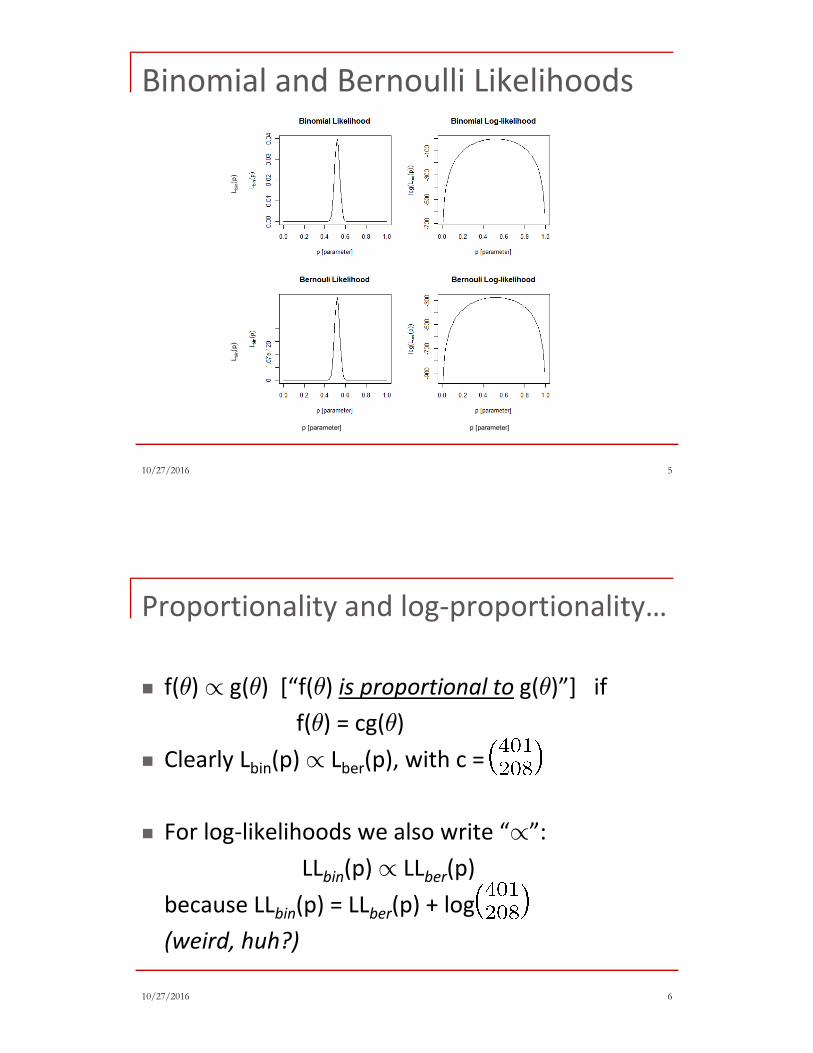
Binomial and Bernoulli Likelihoods

0.0 0.2 0.4 0.6 0.8 1.0

0.0

00

0.0

10

0.0

20

p [parameter]

Lbin(p)

Binomial Likelihood

p [parameter]

Lbin(p)

0.0 0.2 0.4 0.6 0.8 1.0

08.7

7e-2

43

1.7

5e-2

42

Bernouli Likelihood

0.0 0.2 0.4 0.6 0.8 1.0

-1400

-1000

-600

-200

p [parameter]

log(L

bin(p))

Binomial Log-likelihood

0.0 0.2 0.4 0.6 0.8 1.0

-1800

-1400

-1000

-600

p [parameter]

log(L

ber(

p))

Bernouli Log-likelihood

610/27/2016

Proportionality and log-proportionality…

� f(θ) ∝ g(θ) [“f(θ) is proportional to g(θ)”] if

f(θ) = cg(θ)

� Clearly Lbin(p) ∝ Lber(p), with c =

� For log-likelihoods we also write “∝”:

LLbin(p) ∝ LLber(p)

because LLbin(p) = LLber(p) + log

(weird, huh?)

710/27/2016

Finding the MLE…

� If we use the Bernoulli likelihood,

� If we use the Binomial likelihood

� Either way we want to maximize

with k = 208, n=401

810/27/2016

� Differentiating and setting to zero…

� so, clearly,

MLE: Point Estimate

910/27/2016

� First we calculate the expected Information

� and then

� A CI for p is then (0.47,0.57), uncertain who wins!

MLE: Standard Error & CI

1010/27/2016

Bayes’ Rule (a.k.a. Bayes’ Theorem)

� A very simple idea with very powerful

consequences

� We often start with information like P[A|B] and

what we really want is P[B|A]. Bayes’ Theorem

lets us “turn the conditioning around”:

� See http://yudkowsky.net/rational/bayes for a

ton of examples and geeky proselytizing.

1110/27/2016

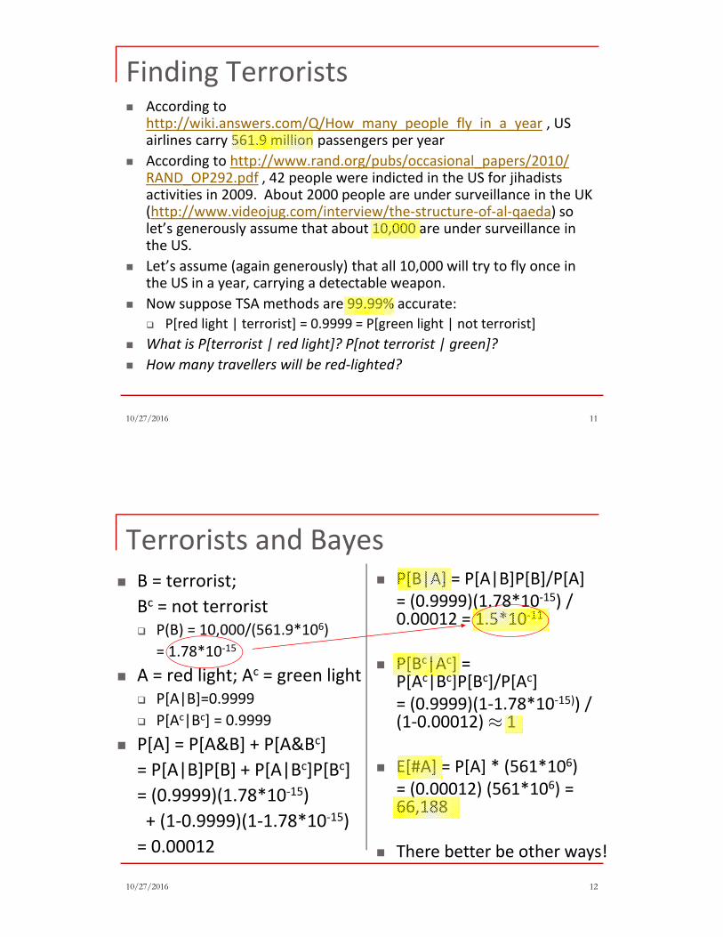
Finding Terrorists� According to

http://wiki.answers.com/Q/How_many_people_fly_in_a_year , US airlines carry 561.9 million passengers per year

� According to http://www.rand.org/pubs/occasional_papers/2010/ RAND_OP292.pdf , 42 people were indicted in the US for jihadists activities in 2009. About 2000 people are under surveillance in the UK (http://www.videojug.com/interview/the-structure-of-al-qaeda) so let’s generously assume that about 10,000 are under surveillance in the US.

� Let’s assume (again generously) that all 10,000 will try to fly once in the US in a year, carrying a detectable weapon.

� Now suppose TSA methods are 99.99% accurate:

� P[red light | terrorist] = 0.9999 = P[green light | not terrorist]

� What is P[terrorist | red light]? P[not terrorist | green]?

� How many travellers will be red-lighted?

1210/27/2016

Terrorists and Bayes

� B = terrorist;

Bc = not terrorist

� P(B) = 10,000/(561.9*106)

= 1.78*10-15

� A = red light; Ac = green light

� P[A|B]=0.9999

� P[Ac|Bc] = 0.9999

� P[A] = P[A&B] + P[A&Bc]

= P[A|B]P[B] + P[A|Bc]P[Bc]

= (0.9999)(1.78*10-15)

+ (1-0.9999)(1-1.78*10-15)

= 0.00012

� P[B|A] = P[A|B]P[B]/P[A]

= (0.9999)(1.78*10-15) / 0.00012 = 1.5*10-11

� P[Bc|Ac] = P[Ac|Bc]P[Bc]/P[Ac]

= (0.9999)(1-1.78*10-15)) / (1-0.00012) ≈ 1

� E[#A] = P[A] * (561*106)

= (0.00012) (561*106) = 66,188

� There better be other ways!

1310/27/2016

Conditional probability & conditional

density

� P[A & B] = P[B|A]P[A]

� P[B] = P[B|A]P[A] +

P[B|Ac]P[Ac]

� P[A|B] = P[A&B]/P[B]

� Bayes’ Theorem:

� f(x,y) = f(y|x) f(x)

�

� f(x|y) = f(x,y)/f(y)

� Bayes’ Theorem:

1410/27/2016

Bayes’ Theorem for Data

� Bayes’ Theorem

� Let x = data, y = θ (parameter!); then

1510/27/2016

Bayes’ Theorem for Data

� We call

� f(θ) the prior distribution

� f(data|θ) = L(θ) the likelihood

� f(θ|data) the posterior distribution

� So Bayes’ Theorem says

� Slogan: (posterior) ∝ (likelihood)×(prior)

1610/27/2016

Back to 2016 Ohio pre-election poll

� The likelihood is the same as before:

L(p) ∝ pk (1-p)n-k

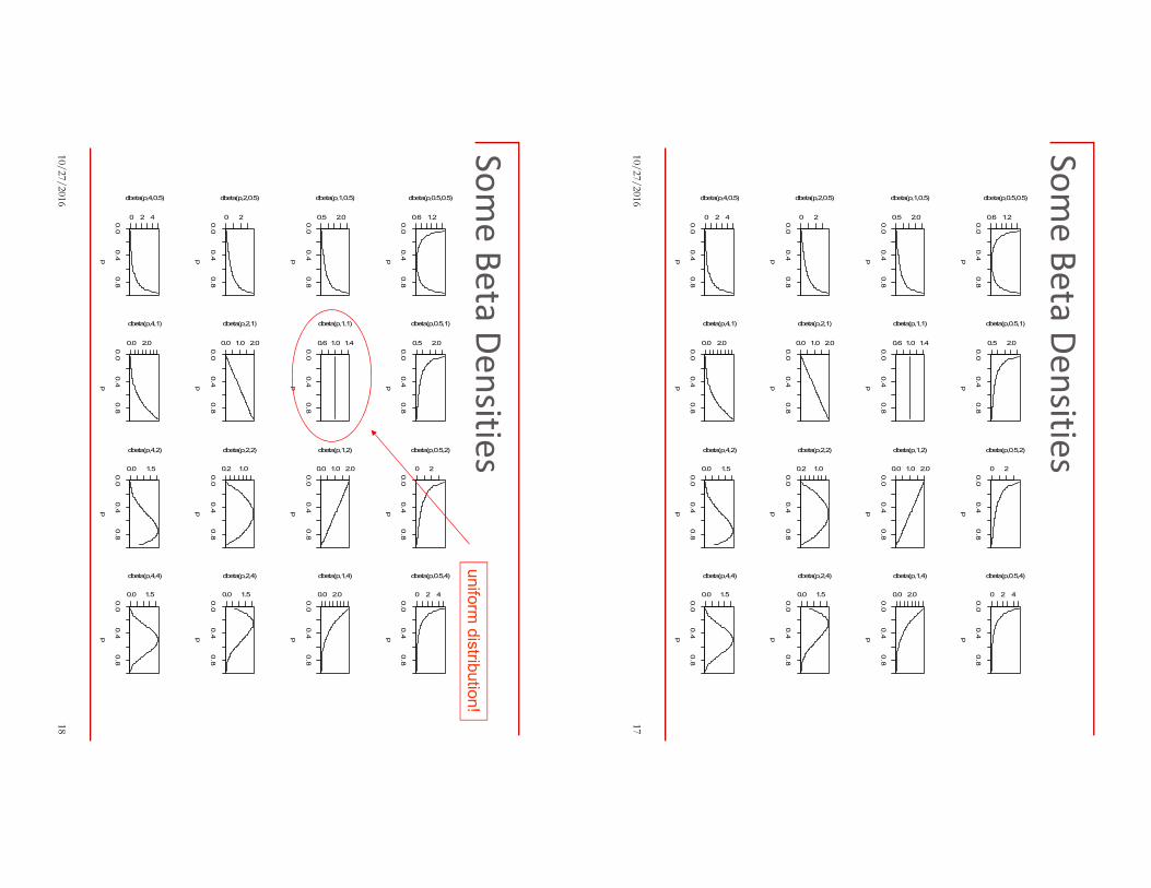
� We need a prior distribution. One good choice is a beta distribution, with

� Some graphs of beta densities appear on the next slide

17

10/27/2016

So

me

Be

ta D

en

sities

0.0

0.4

0.8

0.6 1.2

p

dbeta(p,0.5,0.5)

0.0

0.4

0.8

0.5 2.0

p

dbeta(p,0.5,1)

0.0

0.4

0.8

0 2

p

dbeta(p,0.5,2)

0.0

0.4

0.8

0 2 4

p

dbeta(p,0.5,4)

0.0

0.4

0.8

0.5 2.0

p

dbeta(p,1,0.5)

0.0

0.4

0.8

0.6 1.0 1.4

p

dbeta(p,1,1)

0.0

0.4

0.8

0.0 1.0 2.0

p

dbeta(p,1,2)

0.0

0.4

0.8

0.0 2.0

p

dbeta(p,1,4)

0.0

0.4

0.8

0 2

p

dbeta(p,2,0.5)

0.0

0.4

0.8

0.0 1.0 2.0

p

dbeta(p,2,1)

0.0

0.4

0.8

0.2 1.0

p

dbeta(p,2,2)

0.0

0.4

0.8

0.0 1.5

p

dbeta(p,2,4)

0.0

0.4

0.8

0 2 4

p

dbeta(p,4,0.5)

0.0

0.4

0.8

0.0 2.0

p

dbeta(p,4,1)

0.0

0.4

0.8

0.0 1.5p

dbeta(p,4,2)

0.0

0.4

0.8

0.0 1.5

p

dbeta(p,4,4)

18

10/27/2016

So

me

Be

ta D

en

sities

0.0

0.4

0.8

0.6 1.2

p

dbeta(p,0.5,0.5)

0.0

0.4

0.8

0.5 2.0

p

dbeta(p,0.5,1)

0.0

0.4

0.8

0 2

p

dbeta(p,0.5,2)

0.0

0.4

0.8

0 2 4

p

dbeta(p,0.5,4)

0.0

0.4

0.8

0.5 2.0

p

dbeta(p,1,0.5)

0.0

0.4

0.8

0.6 1.0 1.4

p

dbeta(p,1,1)

0.0

0.4

0.8

0.0 1.0 2.0

p

dbeta(p,1,2)

0.0

0.4

0.8

0.0 2.0

p

dbeta(p,1,4)

0.0

0.4

0.8

0 2

p

dbeta(p,2,0.5)

0.0

0.4

0.8

0.0 1.0 2.0

p

dbeta(p,2,1)

0.0

0.4

0.8

0.2 1.0

p

dbeta(p,2,2)

0.0

0.4

0.8

0.0 1.5

p

dbeta(p,2,4)

0.0

0.4

0.8

0 2 4

p

dbeta(p,4,0.5)

0.0

0.4

0.8

0.0 2.0

p

dbeta(p,4,1)

0.0

0.4

0.8

0.0 1.5

p

dbeta(p,4,2)

0.0

0.4

0.8

0.0 1.5

p

dbeta(p,4,4)

unifo

rm d

istrib

utio

n!

1910/27/2016

Choosing prior parameters…

� The likelihood is the same as before:

L(p) ∝ pk (1-p)n-k = p208(1-p)193

� The prior distribution is a beta distribution

� α = 1, β = 1 gives a uniform distribution – no

preference for one p over another!

� Suppose that in a previous poll, 942 prefer Trump and

1008 prefer Clinton. Could set α=942, β=1008

2010/27/2016

If α=1 and β=1…

� (posterior) ∝ (likelihood)×(prior):

� Since f(p|data)=L(p),

posterior mode = MLE

= 208/401 = 0.52

� Since f(p|data) is a beta

with α=209, β=194,

E[p|data] = 209/403

2110/27/2016

If α=942, β=1008…

� (posterior) ∝ (likelihood)×(prior):

� Since f(p|data) =

beta(p,1150,1202),

E[p|data] = 1150/2352

= 0.489 vs MLE=0.519

“shrinkage”:

posterior between

prior & likelihood

2210/27/2016

Standard Errors (α=942, β=1008)

� Since

then

(compare to SE=0.018 from MLE…)

� Approx 95% interval from :

(0.47, 0.51) … still can’t decide…

2310/27/2016

Alternative interval for p…

� Since we know the posterior distribution of p, we

can calculate the 2.5%-ile and 97.5%-ile and get

another 95% interval:> nsim <- 10000

> p <- rbeta(nsim,1150,1202)

> quantile(p,c(0.025,.5,.975))

2.5% 50% 97.5%

0.4688515 0.4889114 0.5086120

� Gives almost the same 95% interval:

(0.47, 0.51) ... still can’t decide...

2410/27/2016

Summary

� For MLE

� Need a function proportional to L(θ)

� Calculate MLE by setting 0 = LL’(θ)

� Calculate where I(θ) = E[-LL’’(θ)]

� For Bayes

� Need a function proportional to L(θ)

� Need a prior distribution

� Calculate (posterior) ∝ (likelihood)×(prior)

� Calculate posterior mean, SE

� Use formula if you have one

� Use simulation if you don’t!

2510/27/2016

What we did…

� 2016 Pre-election poll in Ohio

� Binomial and Bernoulli MLE

� Bayes’ Rule

� Bayes for densities

� Bayesian inference

� 2016 Pre-election poll in Ohio

� Summary!