3.7 applications of tangent lines
TRANSCRIPT

Applications of Tangent Lines

Applications of Tangent Lines
In this section we look at two applications of the
tangent lines.
Applications of Tangent Lines
In this section we look at two applications of the
tangent lines.
Differentials and Linear Approximation
Applications of Tangent Lines
In this section we look at two applications of the
tangent lines.
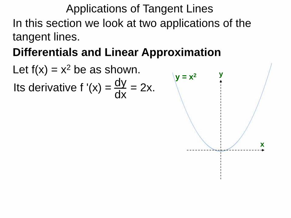
Differentials and Linear Approximation
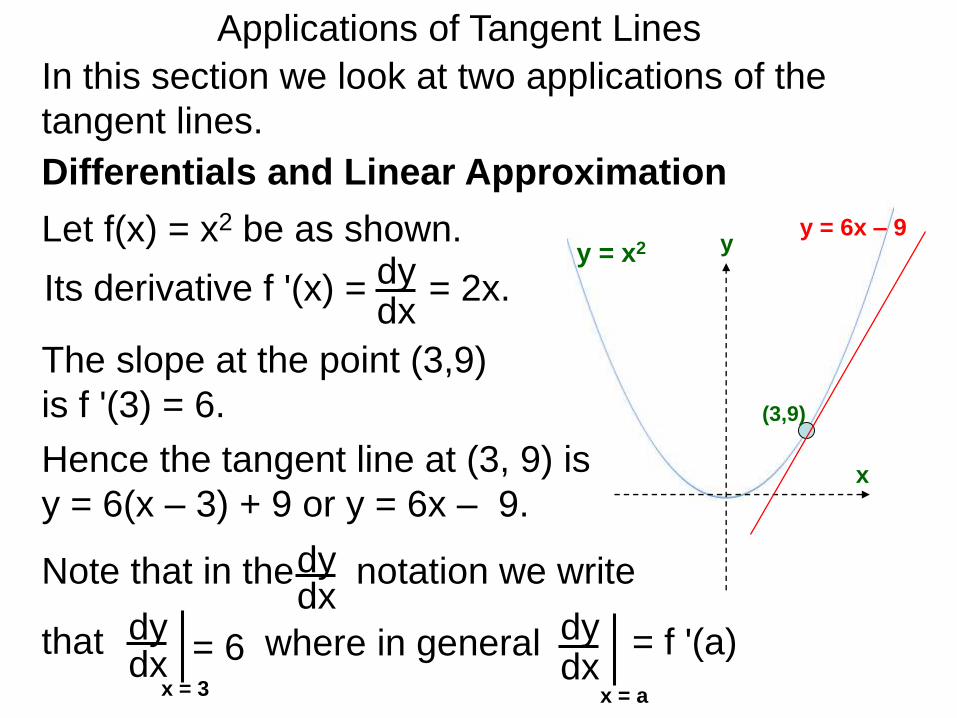
Let f(x) = x2 be as shown. y
Its derivative f '(x) = = 2x. dydx
y = x2
x
Applications of Tangent Lines
In this section we look at two applications of the
tangent lines.
Differentials and Linear Approximation
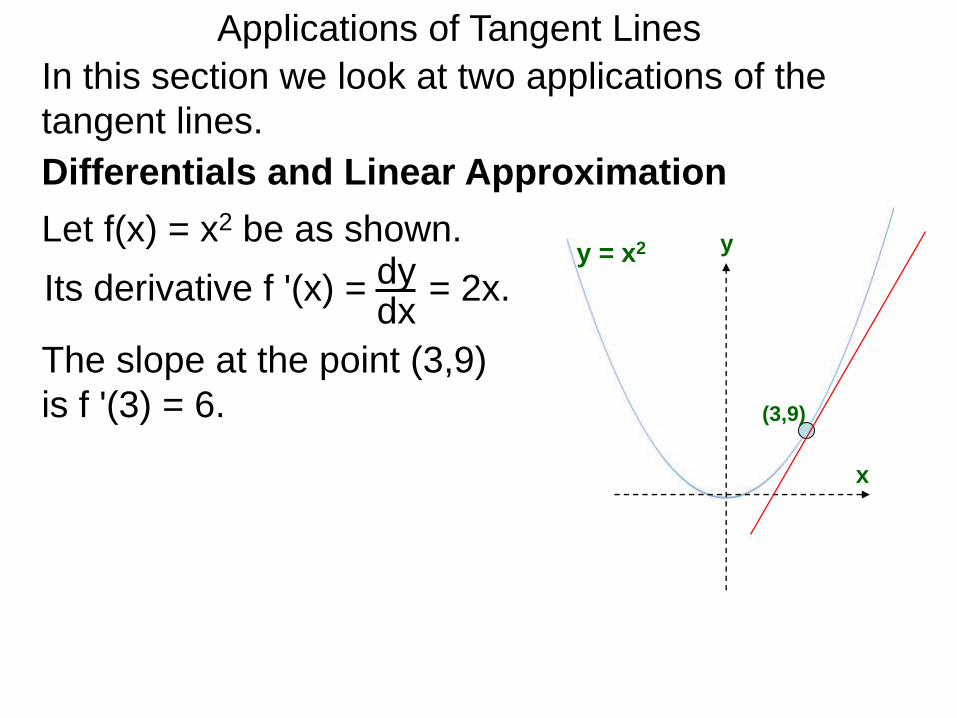
Let f(x) = x2 be as shown. y
Its derivative f '(x) = = 2x.
The slope at the point (3,9)
is f '(3) = 6.
dydx
(3,9)
y = x2
x
Applications of Tangent Lines
In this section we look at two applications of the
tangent lines.
Differentials and Linear Approximation
Let f(x) = x2 be as shown. y
Its derivative f '(x) = = 2x.
The slope at the point (3,9)
is f '(3) = 6.
dydx
(3,9)
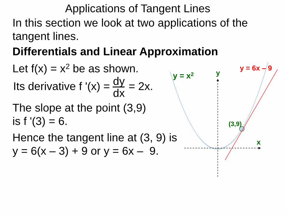
y = x2y = 6x – 9
Hence the tangent line at (3, 9) is
y = 6(x – 3) + 9 or y = 6x – 9.x
Applications of Tangent Lines
In this section we look at two applications of the
tangent lines.
Differentials and Linear Approximation
Let f(x) = x2 be as shown. y
Its derivative f '(x) = = 2x.
The slope at the point (3,9)
is f '(3) = 6.
dydx
(3,9)
y = x2y = 6x – 9
Hence the tangent line at (3, 9) is
y = 6(x – 3) + 9 or y = 6x – 9.
Note that in the notation we write
that
dxdydx
x = 3
= 6dydx
x = a
= f '(a)
dy
where in general
x

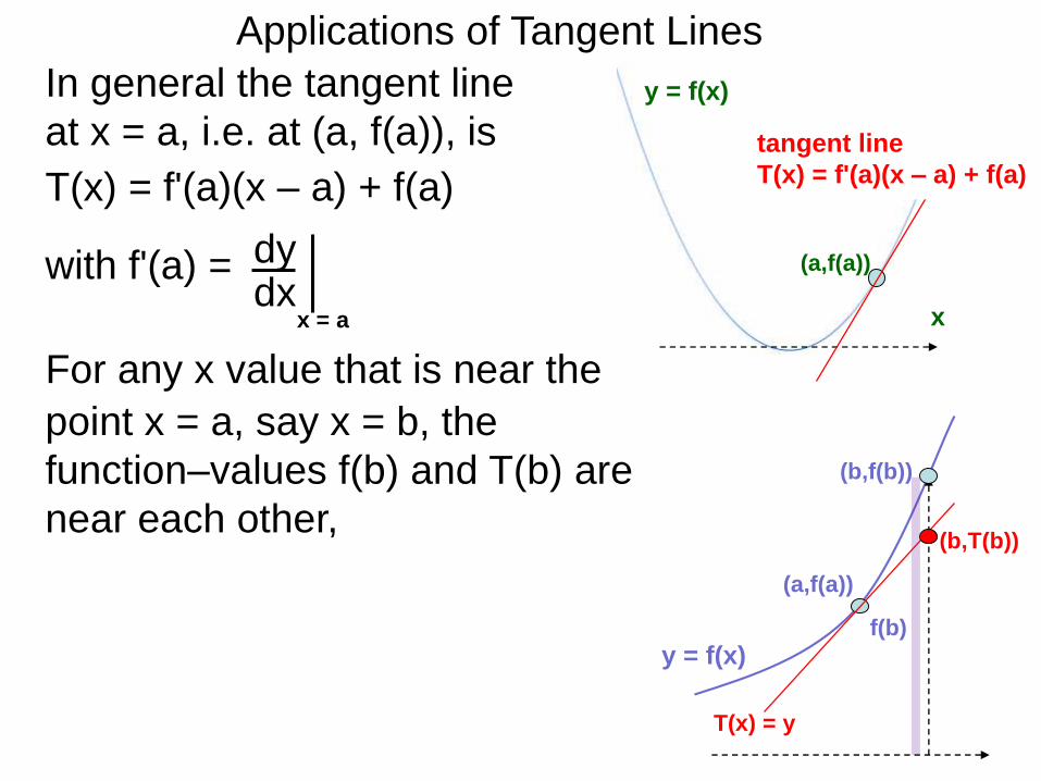
In general the tangent line
at x = a, i.e. at (a, f(a)), is
with f'(a) = dydx
x = a
T(x) = f'(a)(x – a) + f(a)
(a,f(a))
y = f(x)
x
tangent line
T(x) = f'(a)(x – a) + f(a)
Applications of Tangent Lines

In general the tangent line
at x = a, i.e. at (a, f(a)), is
with f'(a) = dydx
x = a
T(x) = f'(a)(x – a) + f(a)
(a,f(a))
y = f(x)
x
tangent line
T(x) = f'(a)(x – a) + f(a)
Applications of Tangent Lines
point x = a, say x = b, the
function–values f(b) and T(b) are
near each other,
For any x value that is near the
(a,f(a))
T(x) = y
(b,f(b))
(b,T(b))
y = f(x)
In general the tangent line
at x = a, i.e. at (a, f(a)), is
with f'(a) = dydx
x = a
T(x) = f'(a)(x – a) + f(a)
(a,f(a))
y = f(x)
x
tangent line
T(x) = f'(a)(x – a) + f(a)
Applications of Tangent Lines
point x = a, say x = b, the
function–values f(b) and T(b) are
near each other,
For any x value that is near the
(a,f(a))
T(x) = y
(b,f(b))
(b,T(b))
y = f(x)f(b)

In general the tangent line
at x = a, i.e. at (a, f(a)), is
with f'(a) = dydx
x = a
T(x) = f'(a)(x – a) + f(a)
(a,f(a))
y = f(x)
x
tangent line
T(x) = f'(a)(x – a) + f(a)
Applications of Tangent Lines
point x = a, say x = b, the
function–values f(b) and T(b) are
near each other,
For any x value that is near the
(a,f(a))
T(x) = y
(b,f(b))
(b,T(b))
y = f(x)T(b) f(b)
In general the tangent line
at x = a, i.e. at (a, f(a)), is
with f'(a) = dydx
x = a
T(x) = f'(a)(x – a) + f(a)
(a,f(a))
y = f(x)
x
tangent line
T(x) = f'(a)(x – a) + f(a)
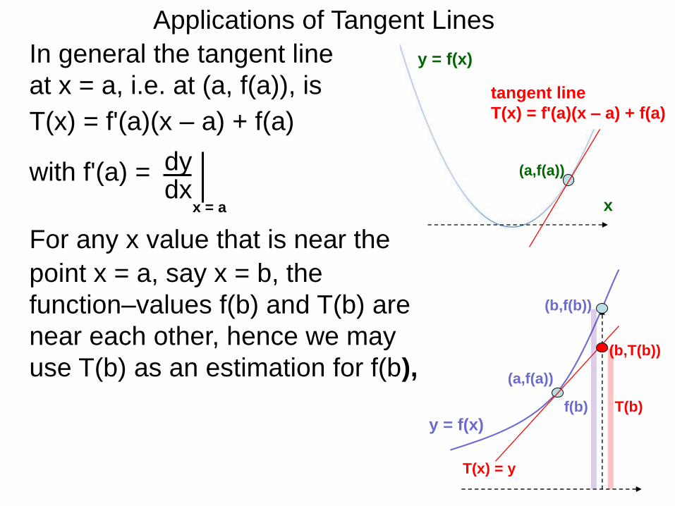
Applications of Tangent Lines
point x = a, say x = b, the
function–values f(b) and T(b) are
near each other, hence we may
use T(b) as an estimation for f(b),
For any x value that is near the
(a,f(a))
T(x) = y
(b,f(b))
(b,T(b))
y = f(x)T(b) f(b)
In general the tangent line
at x = a, i.e. at (a, f(a)), is
with f'(a) = dydx
x = a
T(x) = f'(a)(x – a) + f(a)
(a,f(a))
y = f(x)
x
tangent line
T(x) = f'(a)(x – a) + f(a)
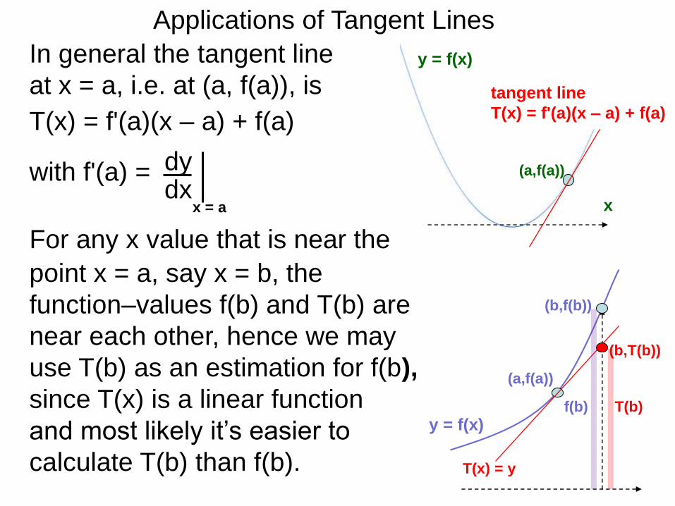
Applications of Tangent Lines
point x = a, say x = b, the
function–values f(b) and T(b) are
near each other, hence we may
use T(b) as an estimation for f(b),
since T(x) is a linear function
and most likely it’s easier to
calculate T(b) than f(b).
For any x value that is near the
(a,f(a))
T(x) = y
(b,f(b))
(b,T(b))
y = f(x)T(b) f(b)

Applications of Tangent Lines
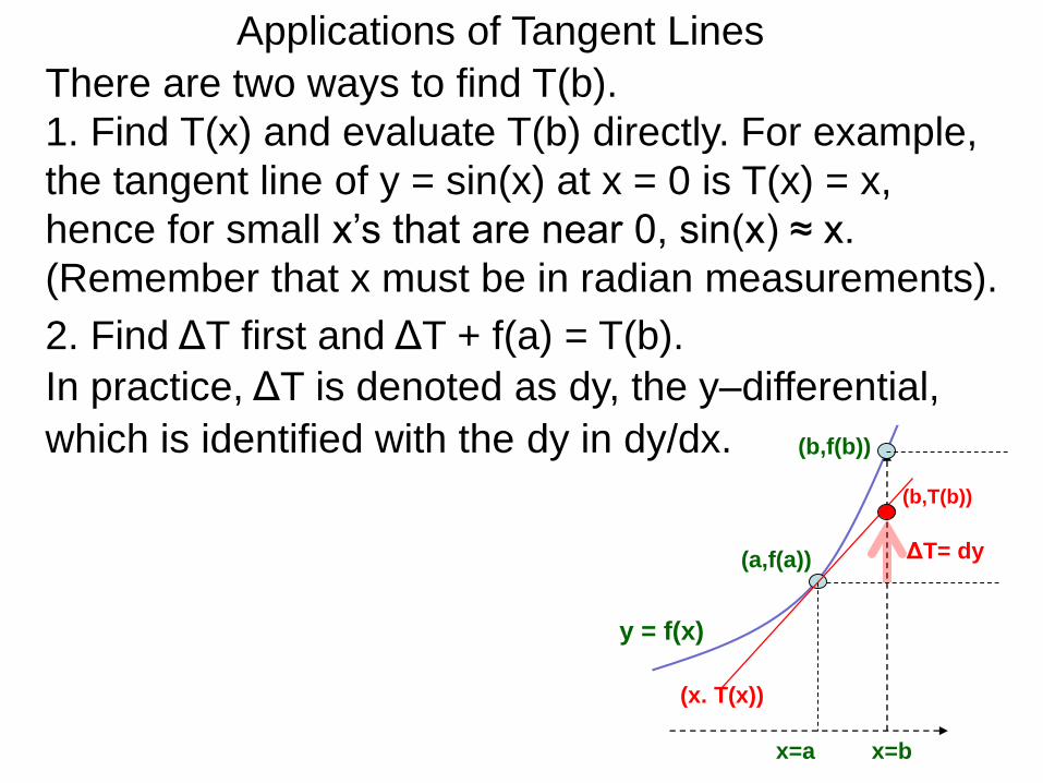
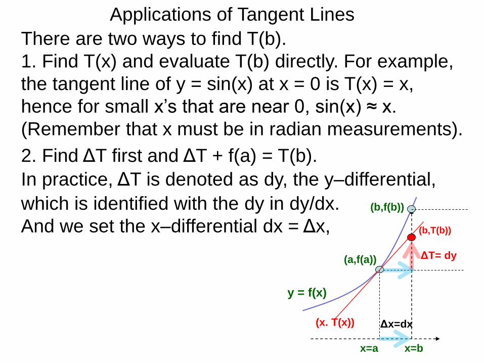
There are two ways to find T(b).

Applications of Tangent Lines
There are two ways to find T(b).
1. Find T(x) and evaluate T(b) directly.
Applications of Tangent Lines
There are two ways to find T(b).
1. Find T(x) and evaluate T(b) directly. For example,
the tangent line of y = sin(x) at x = 0 is T(x) = x,
Applications of Tangent Lines
There are two ways to find T(b).
1. Find T(x) and evaluate T(b) directly. For example,
the tangent line of y = sin(x) at x = 0 is T(x) = x,
hence for small x’s that are near 0, sin(x) ≈ x.
(Remember that x must be in radian measurements).
Applications of Tangent Lines
There are two ways to find T(b).
1. Find T(x) and evaluate T(b) directly. For example,
the tangent line of y = sin(x) at x = 0 is T(x) = x,
hence for small x’s that are near 0, sin(x) ≈ x.
(Remember that x must be in radian measurements).
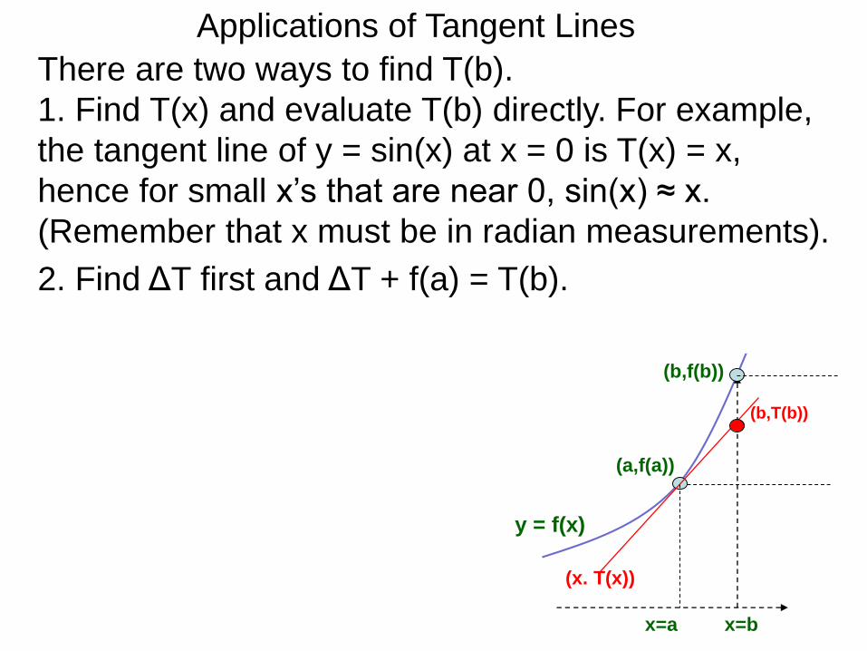
(a,f(a))
(x. T(x))
(b,f(b))
(b,T(b))
y = f(x)
x=a x=b
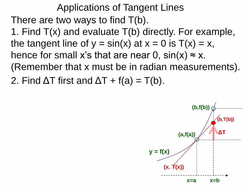
2. Find ΔT first and ΔT + f(a) = T(b).
Applications of Tangent Lines
There are two ways to find T(b).
1. Find T(x) and evaluate T(b) directly. For example,
the tangent line of y = sin(x) at x = 0 is T(x) = x,
hence for small x’s that are near 0, sin(x) ≈ x.
(Remember that x must be in radian measurements).
(a,f(a))
(x. T(x))
(b,f(b))
(b,T(b))
y = f(x)
x=a
ΔT
x=b
2. Find ΔT first and ΔT + f(a) = T(b).
Applications of Tangent Lines
There are two ways to find T(b).
1. Find T(x) and evaluate T(b) directly. For example,
the tangent line of y = sin(x) at x = 0 is T(x) = x,
hence for small x’s that are near 0, sin(x) ≈ x.
(Remember that x must be in radian measurements).
which is identified with the dy in dy/dx.
(a,f(a))
(x. T(x))
(b,f(b))
(b,T(b))
y = f(x)
x=a
ΔT= dy
x=b
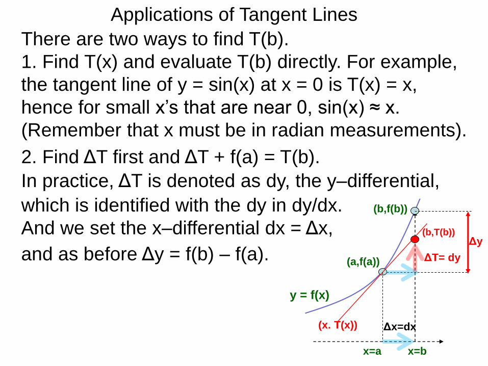
2. Find ΔT first and ΔT + f(a) = T(b).
In practice, ΔT is denoted as dy, the y–differential,
Applications of Tangent Lines
There are two ways to find T(b).
1. Find T(x) and evaluate T(b) directly. For example,
the tangent line of y = sin(x) at x = 0 is T(x) = x,
hence for small x’s that are near 0, sin(x) ≈ x.
(Remember that x must be in radian measurements).
which is identified with the dy in dy/dx.
And we set the x–differential dx = Δx,
(a,f(a))
(x. T(x))
(b,f(b))
(b,T(b))
y = f(x)
x=a
Δx=dx
ΔT= dy
x=b
2. Find ΔT first and ΔT + f(a) = T(b).
In practice, ΔT is denoted as dy, the y–differential,
Applications of Tangent Lines
There are two ways to find T(b).
1. Find T(x) and evaluate T(b) directly. For example,
the tangent line of y = sin(x) at x = 0 is T(x) = x,
hence for small x’s that are near 0, sin(x) ≈ x.
(Remember that x must be in radian measurements).
which is identified with the dy in dy/dx.
And we set the x–differential dx = Δx,
and as before Δy = f(b) – f(a). (a,f(a))
(x. T(x))
(b,f(b))
(b,T(b))
y = f(x)
x=a
Δx=dx
ΔT= dy
x=b
2. Find ΔT first and ΔT + f(a) = T(b).
In practice, ΔT is denoted as dy, the y–differential,
Δy

Applications of Tangent Lines
There are two ways to find T(b).
1. Find T(x) and evaluate T(b) directly. For example,
the tangent line of y = sin(x) at x = 0 is T(x) = x,
hence for small x’s that are near 0, sin(x) ≈ x.
(Remember that x must be in radian measurements).
which is identified with the dy in dy/dx.
And we set the x–differential dx = Δx,
and as before Δy = f(b) – f(a).
These measurements are
shown here. It’s important to
(a,f(a))
(x. T(x))
(b,f(b))
(b,T(b))
y = f(x)
x=a
Δx=dx
ΔT= dy
x=b
Δy
2. Find ΔT first and ΔT + f(a) = T(b).
In practice, ΔT is denoted as dy, the y–differential,
“see” them because the
geometry is linked to the algebra.
Applications of Tangent Lines
(a,f(a))
(x. T(x))
(b,f(b))
(b,T(b))
y = f(x)
x=a
Δx=dx
ΔT= dy
x=b
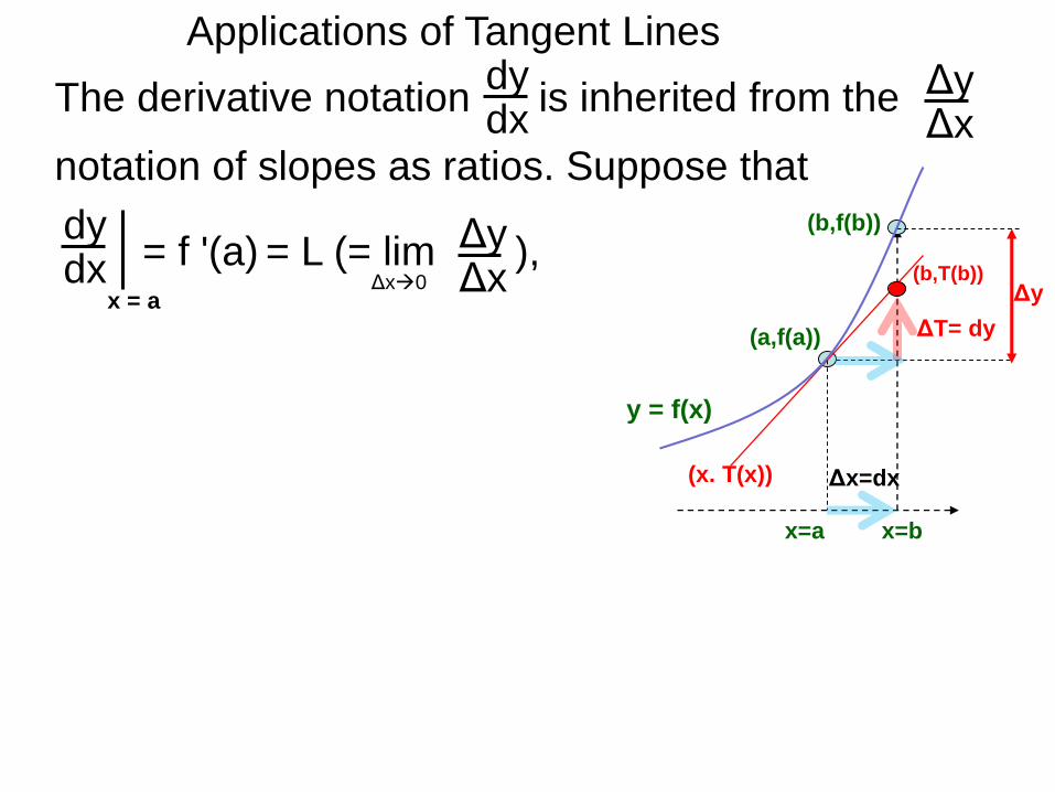
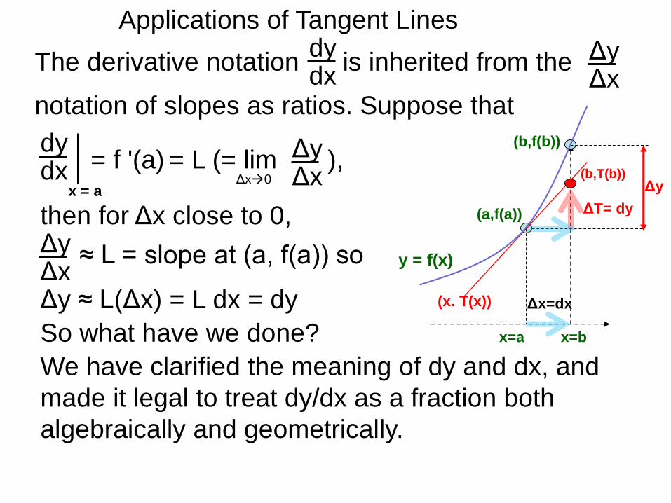
Δy
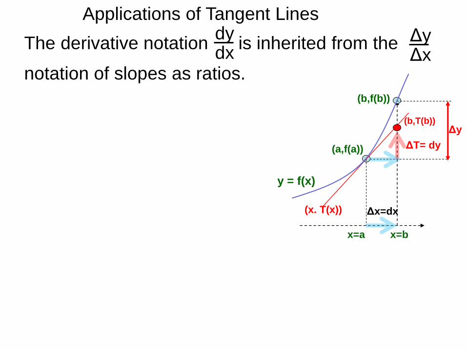
The derivative notation is inherited from the
notation of slopes as ratios.
dydx
ΔyΔx
Applications of Tangent Lines
Δx0= L (= lim ),
(a,f(a))
(x. T(x))
(b,f(b))
(b,T(b))
y = f(x)
x=a
Δx=dx
ΔT= dy
x=b
Δy
dydx
x = a
= f '(a) ΔyΔx
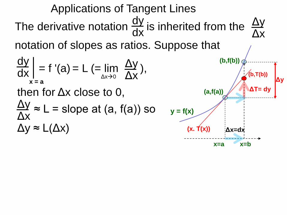
The derivative notation is inherited from the
notation of slopes as ratios. Suppose that
dydx
ΔyΔx

Applications of Tangent Lines
Δx0= L (= lim ),
ΔyΔx
then for Δx close to 0, (a,f(a))
(x. T(x))
(b,f(b))
(b,T(b))
y = f(x)
x=a
Δx=dx
ΔT= dy
x=b
Δy
dydx
x = a
= f '(a) ΔyΔx
≈ L = slope at (a, f(a))
The derivative notation is inherited from the
notation of slopes as ratios. Suppose that
dydx
ΔyΔx
Applications of Tangent Lines
Δx0= L (= lim ),
ΔyΔx
then for Δx close to 0, (a,f(a))
(x. T(x))
(b,f(b))
(b,T(b))
y = f(x)
x=a
Δx=dx
ΔT= dy
x=b
Δy
Δy ≈ L(Δx)
dydx
x = a
= f '(a) ΔyΔx
≈ L = slope at (a, f(a)) so
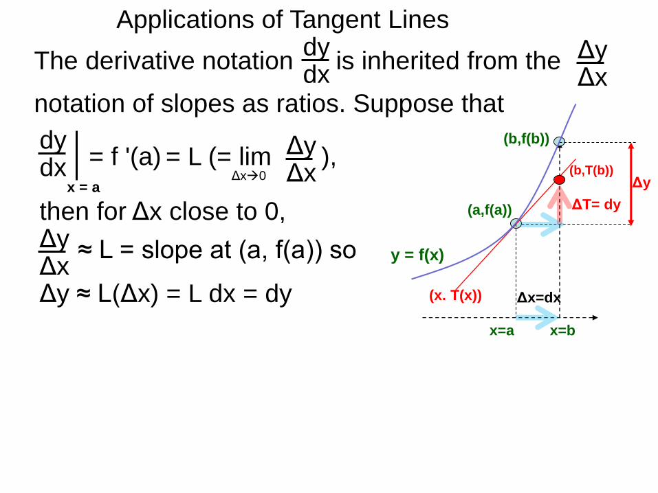
The derivative notation is inherited from the
notation of slopes as ratios. Suppose that
dydx
ΔyΔx
Applications of Tangent Lines
Δx0= L (= lim ),
ΔyΔx
then for Δx close to 0, (a,f(a))
(x. T(x))
(b,f(b))
(b,T(b))
y = f(x)
x=a
Δx=dx
ΔT= dy
x=b
Δy
Δy ≈ L(Δx) = L dx = dy
dydx
x = a
= f '(a) ΔyΔx
≈ L = slope at (a, f(a)) so
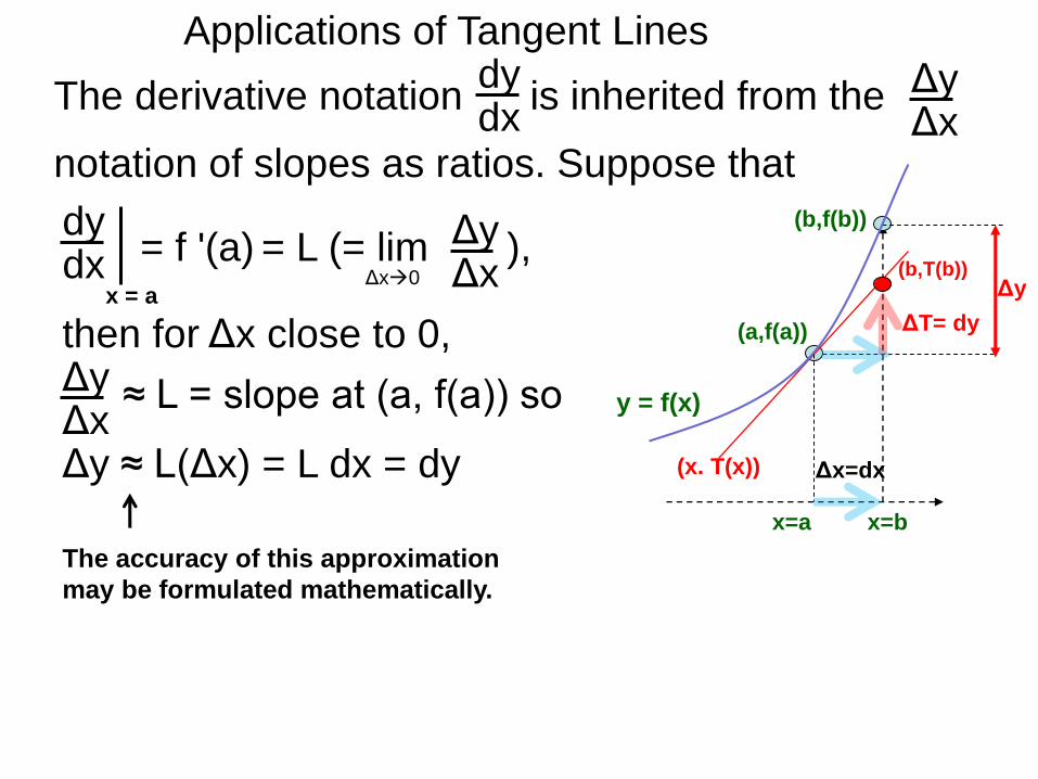
The derivative notation is inherited from the
notation of slopes as ratios. Suppose that
dydx
ΔyΔx
Applications of Tangent Lines
Δx0= L (= lim ),
ΔyΔx
then for Δx close to 0, (a,f(a))
(x. T(x))
(b,f(b))
(b,T(b))
y = f(x)
x=a
Δx=dx
ΔT= dy
x=b
Δy
Δy ≈ L(Δx) = L dx = dy
dydx
x = a
= f '(a) ΔyΔx
The accuracy of this approximation
may be formulated mathematically.
≈ L = slope at (a, f(a)) so
The derivative notation is inherited from the
notation of slopes as ratios. Suppose that
dydx
ΔyΔx
The derivative notation is inherited from the
notation of slopes as ratios. Suppose that
Applications of Tangent Linesdydx
ΔyΔx
Δx0= L (= lim ),
ΔyΔx
≈ L = slope at (a, f(a)) so
then for Δx close to 0, (a,f(a))
(x. T(x))
(b,f(b))
(b,T(b))
y = f(x)
x=a
Δx=dx
ΔT= dy
x=b
Δy
Δy ≈ L(Δx) = L dx = dy
dydx
x = a
= f '(a) ΔyΔx
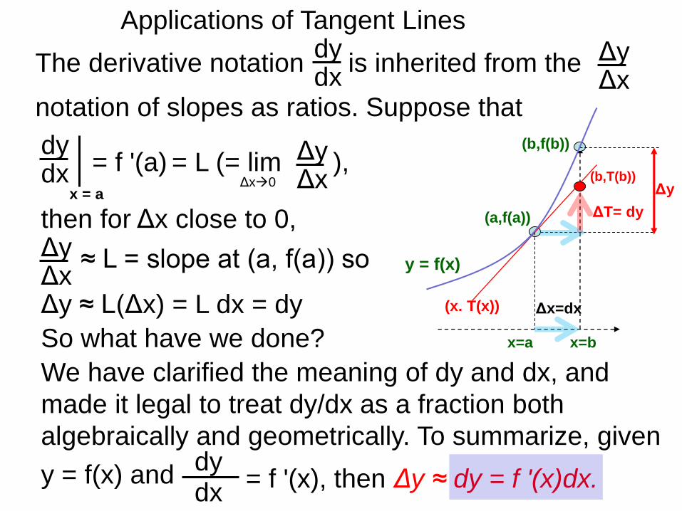
So what have we done?
We have clarified the meaning of dy and dx, and
made it legal to treat dy/dx as a fraction both
algebraically and geometrically.
The derivative notation is inherited from the
notation of slopes as ratios. Suppose that
Applications of Tangent Linesdydx
ΔyΔx
Δx0= L (= lim ),
ΔyΔx
≈ L = slope at (a, f(a)) so
then for Δx close to 0, (a,f(a))
(x. T(x))
(b,f(b))
(b,T(b))
y = f(x)
x=a
Δx=dx
ΔT= dy
x=b
Δy
Δy ≈ L(Δx) = L dx = dy
dydx
x = a
= f '(a) ΔyΔx
So what have we done?
We have clarified the meaning of dy and dx, and
made it legal to treat dy/dx as a fraction both
algebraically and geometrically. To summarize, given dydx
= f '(x), then Δy ≈ dy = f '(x)dx.y = f(x) and
Applications of Tangent Lines
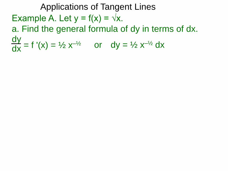
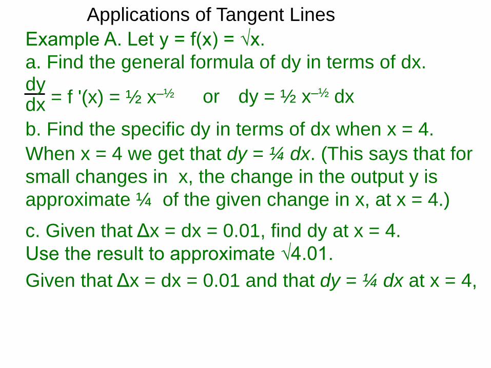
Example A. Let y = f(x) = √x.
a. Find the general formula of dy in terms of dx.
Applications of Tangent Lines
Example A. Let y = f(x) = √x.
a. Find the general formula of dy in terms of dx.dydx = f '(x) = ½ x–½
Applications of Tangent Lines
Example A. Let y = f(x) = √x.
a. Find the general formula of dy in terms of dx.dydx = f '(x) = ½ x–½ or dy = ½ x–½ dx

Applications of Tangent Lines
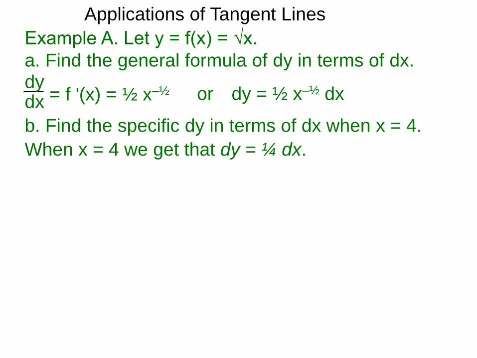
Example A. Let y = f(x) = √x.
a. Find the general formula of dy in terms of dx.
b. Find the specific dy in terms of dx when x = 4.
dydx = f '(x) = ½ x–½ or dy = ½ x–½ dx
Applications of Tangent Lines
Example A. Let y = f(x) = √x.
a. Find the general formula of dy in terms of dx.
b. Find the specific dy in terms of dx when x = 4.
dydx = f '(x) = ½ x–½ or dy = ½ x–½ dx
When x = 4 we get that dy = ¼ dx.
Applications of Tangent Lines
Example A. Let y = f(x) = √x.
a. Find the general formula of dy in terms of dx.
b. Find the specific dy in terms of dx when x = 4.
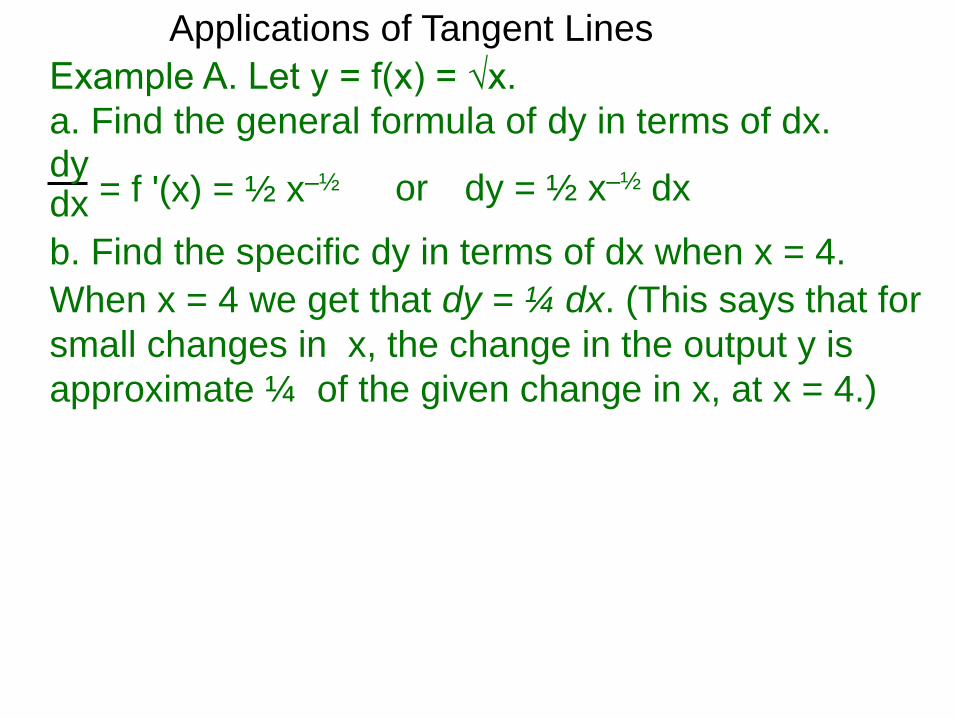
dydx = f '(x) = ½ x–½ or dy = ½ x–½ dx
When x = 4 we get that dy = ¼ dx. (This says that for
small changes in x, the change in the output y is
approximate ¼ of the given change in x, at x = 4.)
Applications of Tangent Lines
Example A. Let y = f(x) = √x.
a. Find the general formula of dy in terms of dx.
b. Find the specific dy in terms of dx when x = 4.
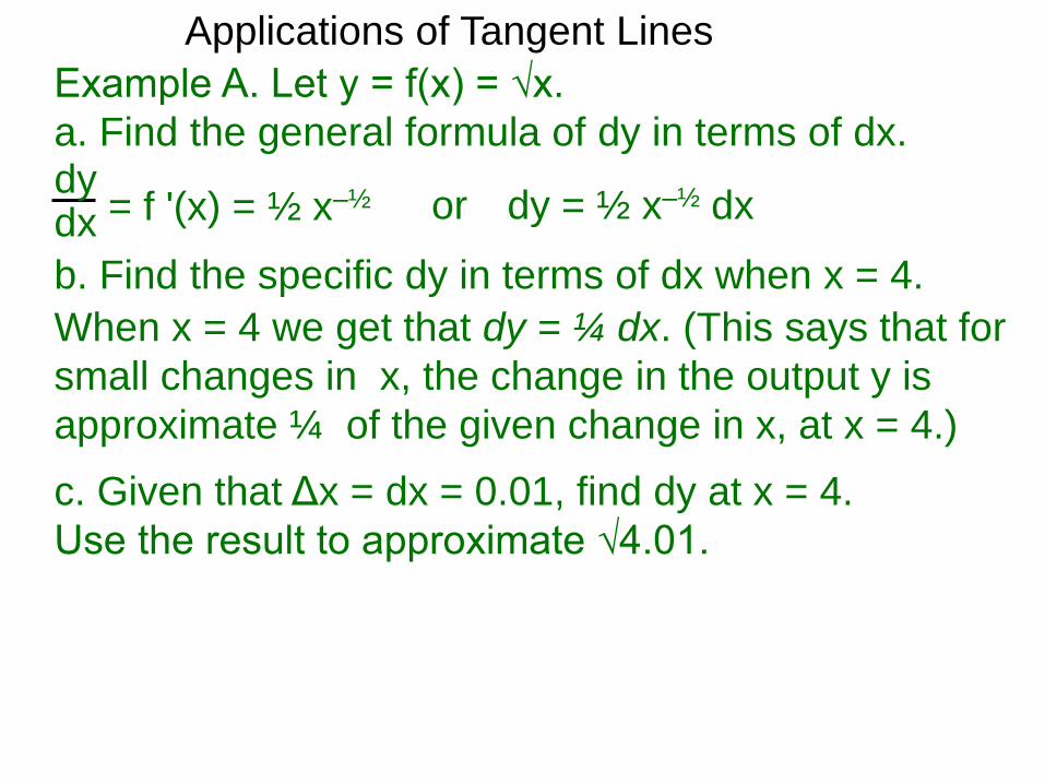
c. Given that Δx = dx = 0.01, find dy at x = 4.
Use the result to approximate √4.01.
dydx = f '(x) = ½ x–½ or dy = ½ x–½ dx
When x = 4 we get that dy = ¼ dx. (This says that for
small changes in x, the change in the output y is
approximate ¼ of the given change in x, at x = 4.)
Applications of Tangent Lines
Example A. Let y = f(x) = √x.
a. Find the general formula of dy in terms of dx.
b. Find the specific dy in terms of dx when x = 4.
c. Given that Δx = dx = 0.01, find dy at x = 4.
Use the result to approximate √4.01.
dydx = f '(x) = ½ x–½ or dy = ½ x–½ dx
When x = 4 we get that dy = ¼ dx. (This says that for
small changes in x, the change in the output y is
approximate ¼ of the given change in x, at x = 4.)
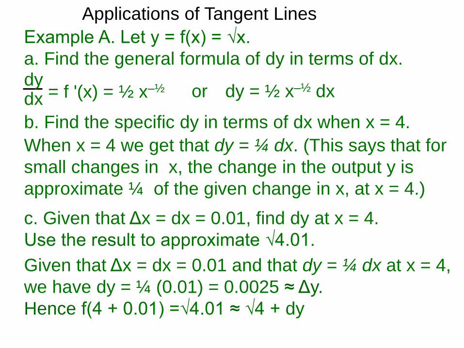
Given that Δx = dx = 0.01 and that dy = ¼ dx at x = 4,

Applications of Tangent Lines
Example A. Let y = f(x) = √x.
a. Find the general formula of dy in terms of dx.
b. Find the specific dy in terms of dx when x = 4.
c. Given that Δx = dx = 0.01, find dy at x = 4.
Use the result to approximate √4.01.
dydx = f '(x) = ½ x–½ or dy = ½ x–½ dx
When x = 4 we get that dy = ¼ dx. (This says that for
small changes in x, the change in the output y is
approximate ¼ of the given change in x, at x = 4.)
Given that Δx = dx = 0.01 and that dy = ¼ dx at x = 4,
we have dy = ¼ (0.01) = 0.0025 ≈ Δy.
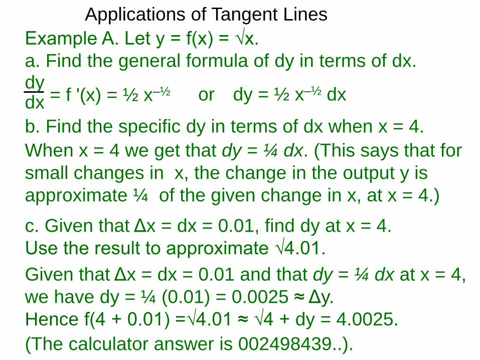
Hence f(4 + 0.01) =√4.01 ≈ √4 + dy
Applications of Tangent Lines
Example A. Let y = f(x) = √x.
a. Find the general formula of dy in terms of dx.
b. Find the specific dy in terms of dx when x = 4.
c. Given that Δx = dx = 0.01, find dy at x = 4.
Use the result to approximate √4.01.
dydx = f '(x) = ½ x–½ or dy = ½ x–½ dx
When x = 4 we get that dy = ¼ dx. (This says that for
small changes in x, the change in the output y is
approximate ¼ of the given change in x, at x = 4.)
Given that Δx = dx = 0.01 and that dy = ¼ dx at x = 4,
we have dy = ¼ (0.01) = 0.0025 ≈ Δy.
Hence f(4 + 0.01) =√4.01 ≈ √4 + dy = 4.0025.
(The calculator answer is 002498439..).
Your turn. Do the same at x = 9, and use the result to
approximate √8.995. What is the dx?
Applications of Tangent Lines
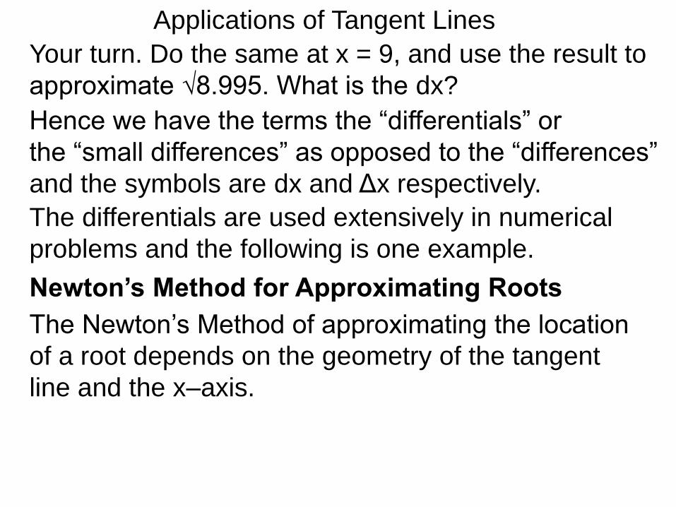
Your turn. Do the same at x = 9, and use the result to
approximate √8.995. What is the dx?
Applications of Tangent Lines
Hence we have the terms the “differentials” or
the “small differences” as opposed to the “differences”
Your turn. Do the same at x = 9, and use the result to
approximate √8.995. What is the dx?
Applications of Tangent Lines
Hence we have the terms the “differentials” or
the “small differences” as opposed to the “differences”
and the symbols are dx and Δx respectively.
Your turn. Do the same at x = 9, and use the result to
approximate √8.995. What is the dx?
Applications of Tangent Lines
Hence we have the terms the “differentials” or
the “small differences” as opposed to the “differences”
and the symbols are dx and Δx respectively.
The differentials are used extensively in numerical
problems and the following is one example.
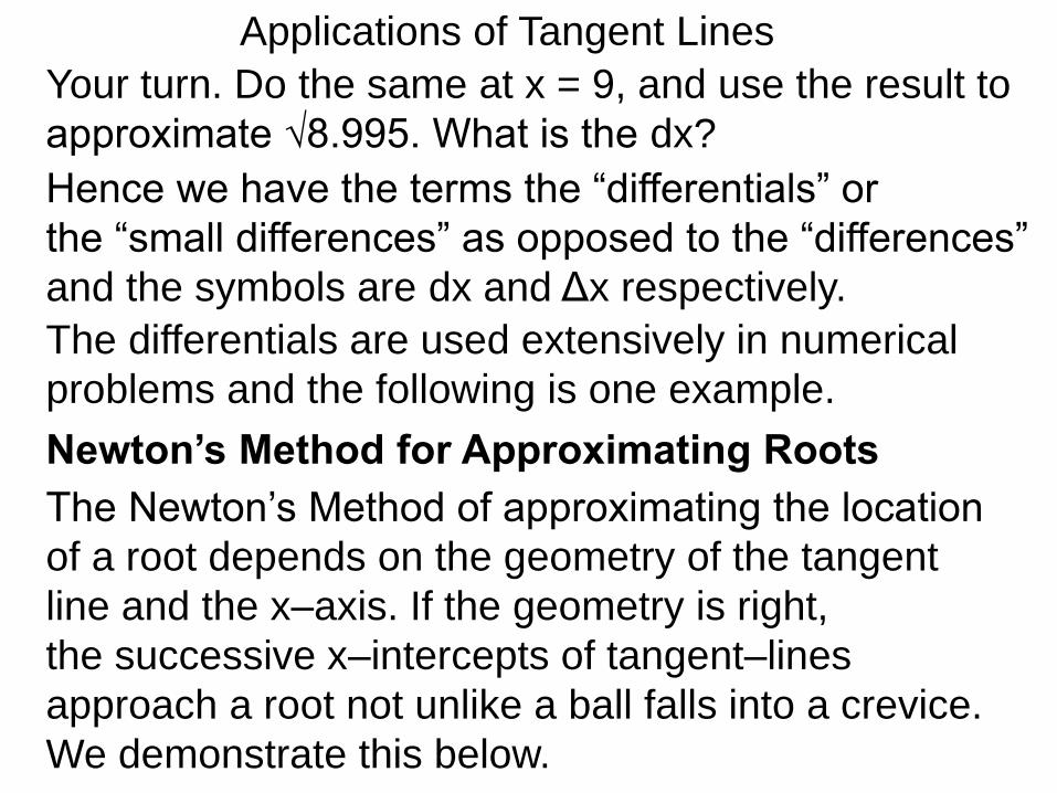
Newton’s Method for Approximating Roots
Your turn. Do the same at x = 9, and use the result to
approximate √8.995. What is the dx?
Applications of Tangent Lines
Hence we have the terms the “differentials” or
the “small differences” as opposed to the “differences”
and the symbols are dx and Δx respectively.
The differentials are used extensively in numerical
problems and the following is one example.
Newton’s Method for Approximating Roots
The Newton’s Method of approximating the location
of a root depends on the geometry of the tangent
line and the x–axis.
Your turn. Do the same at x = 9, and use the result to
approximate √8.995. What is the dx?
Applications of Tangent Lines
Hence we have the terms the “differentials” or
the “small differences” as opposed to the “differences”
and the symbols are dx and Δx respectively.
The differentials are used extensively in numerical
problems and the following is one example.
Newton’s Method for Approximating Roots
The Newton’s Method of approximating the location
of a root depends on the geometry of the tangent
line and the x–axis. If the geometry is right,
the successive x–intercepts of tangent–lines
approach a root not unlike a ball falls into a crevice.
We demonstrate this below.
Applications of Tangent Lines
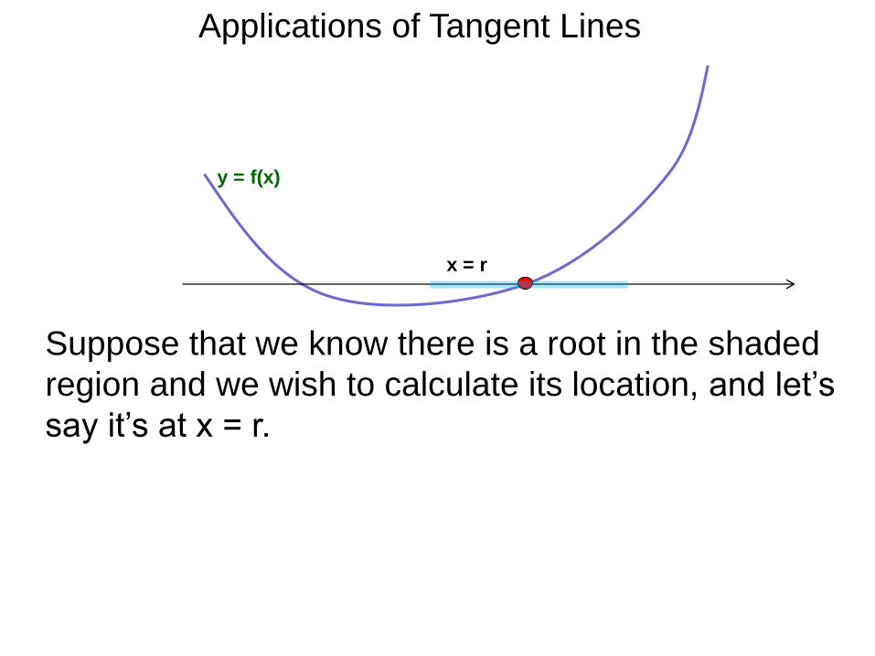
Suppose that we know there is a root in the shaded
region and we wish to calculate its location, and let’s
say it’s at x = r.
y = f(x)
x = r
Applications of Tangent Lines
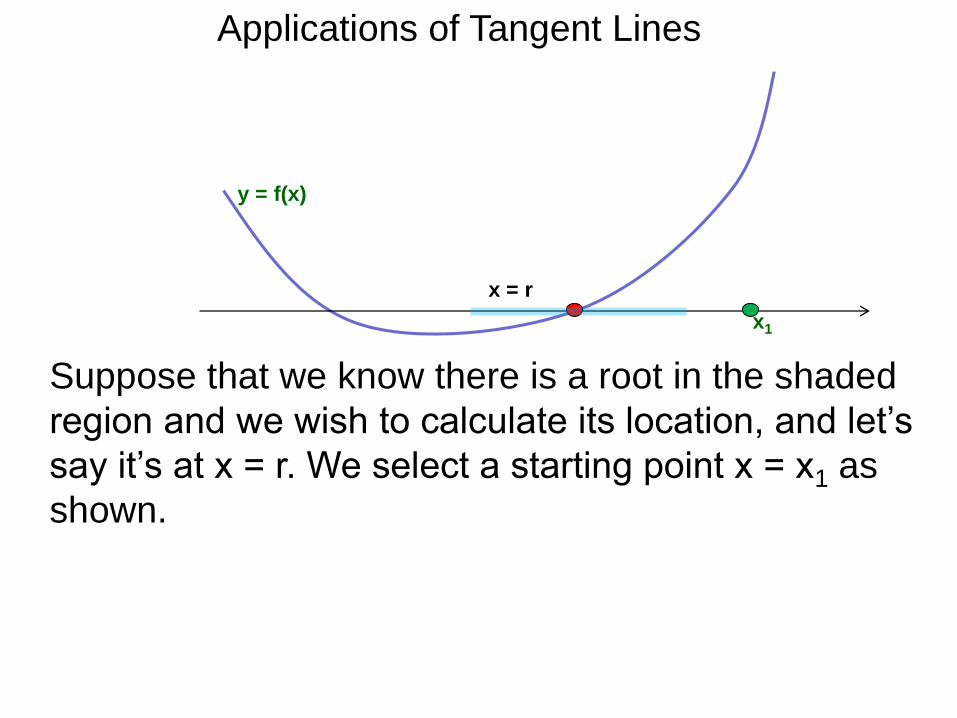
Suppose that we know there is a root in the shaded
region and we wish to calculate its location, and let’s
say it’s at x = r. We select a starting point x = x1 as
shown.
y = f(x)
x = r
x1
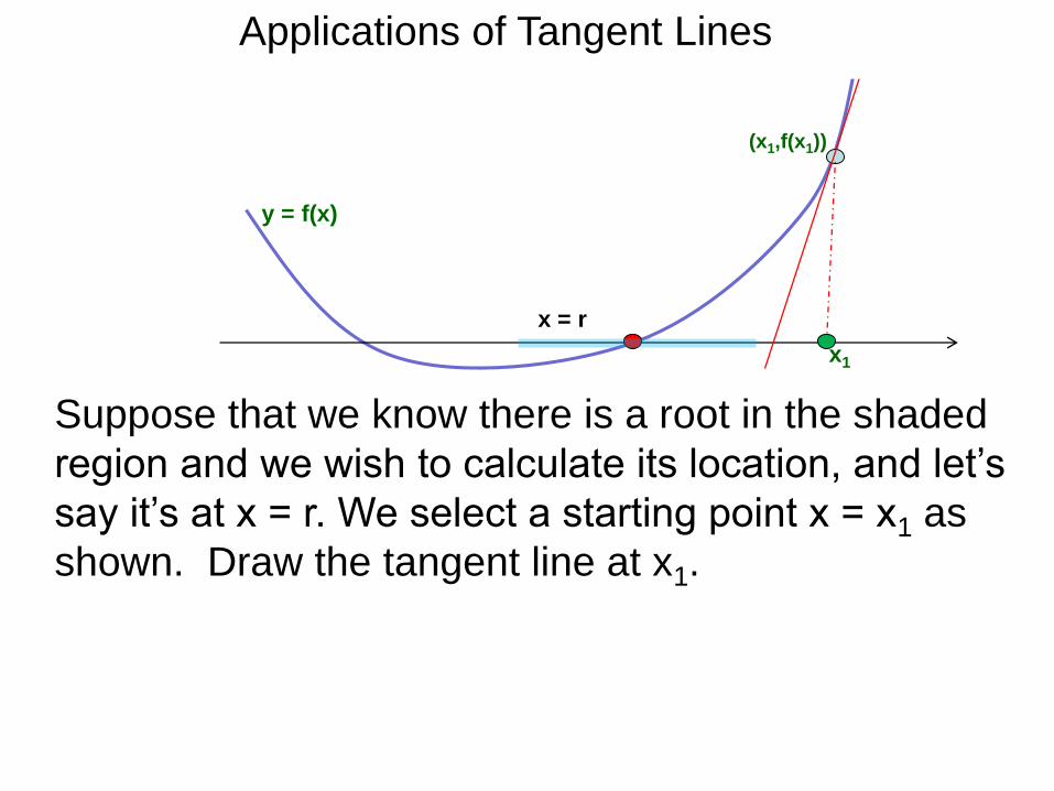
Applications of Tangent Lines
Suppose that we know there is a root in the shaded
region and we wish to calculate its location, and let’s
say it’s at x = r. We select a starting point x = x1 as
shown. Draw the tangent line at x1.
(x1,f(x1))
y = f(x)
x = r
x1
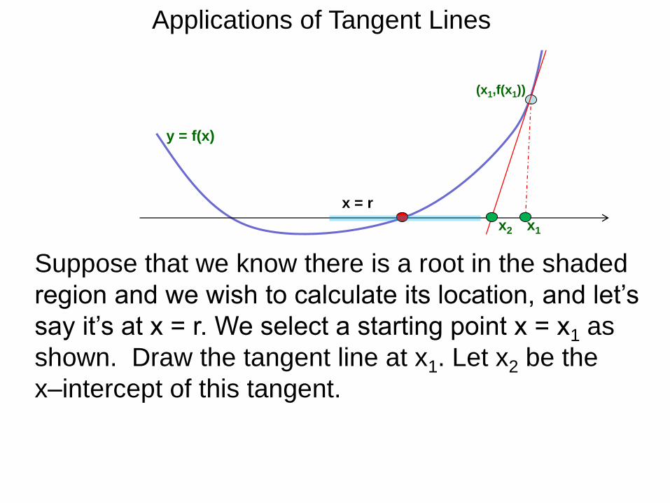
Applications of Tangent Lines
Suppose that we know there is a root in the shaded
region and we wish to calculate its location, and let’s
say it’s at x = r. We select a starting point x = x1 as
shown. Draw the tangent line at x1. Let x2 be the
x–intercept of this tangent.
(x1,f(x1))
y = f(x)
x = r
x1x2
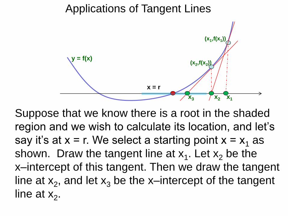
Applications of Tangent Lines
Suppose that we know there is a root in the shaded
region and we wish to calculate its location, and let’s
say it’s at x = r. We select a starting point x = x1 as
shown. Draw the tangent line at x1. Let x2 be the
x–intercept of this tangent. Then we draw the tangent
line at x2, and let x3 be the x–intercept of the tangent
line at x2.
(x1,f(x1))
y = f(x)
x = r
x1x3 x2
(x2,f(x2))

Applications of Tangent Lines
Suppose that we know there is a root in the shaded
region and we wish to calculate its location, and let’s
say it’s at x = r. We select a starting point x = x1 as
shown. Draw the tangent line at x1. Let x2 be the
x–intercept of this tangent. Then we draw the tangent
line at x2, and let x3 be the x–intercept of the tangent
line at x2. Continuing in this manner, the sequence of
x’s is funneled toward the root x = r.
(x1,f(x1))
y = f(x)
x = r
x1x3 x2
(x3,f(x3))
(x2,f(x2))
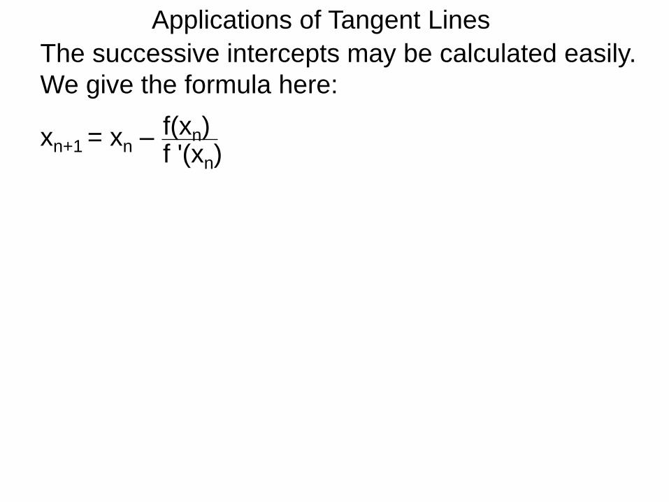
Applications of Tangent Lines
The successive intercepts may be calculated easily.
We give the formula here:
xn+1 = xn – f(xn)f '(xn)

Applications of Tangent Lines
The successive intercepts may be calculated easily.
We give the formula here:
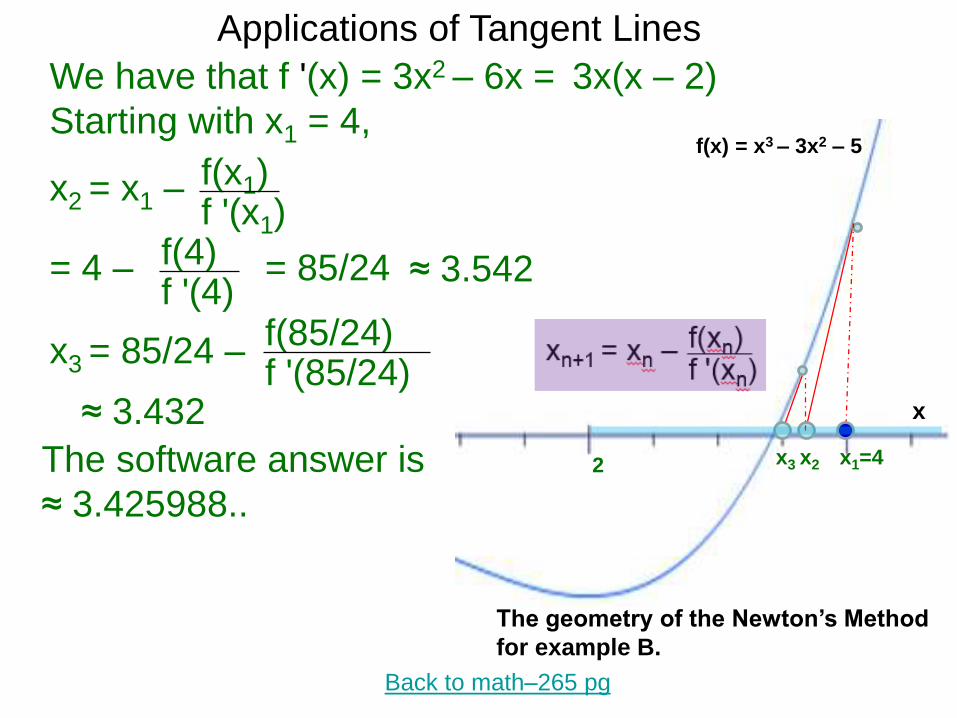
Example B.
Let y = f(x) = x3 – 3x2 – 5, its
graph is shown here. Assume
that we know that it has a root
between 2 < x < 5.
Starting with x1 = 4,
approximate this roots by the
Newton’s method to x3.
Compare this with a calculator
answer.
xn+1 = xn – f(xn)f '(xn)
2 4
y
x
f(x) = x3 – 3x2 – 5
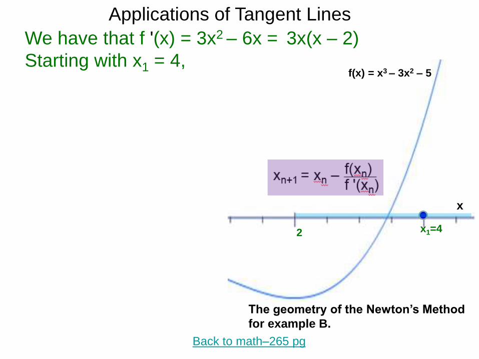
Applications of Tangent Lines
We have that f '(x) = 3x2 – 6x = 3x(x – 2)
Starting with x1 = 4,
x1=42
x
f(x) = x3 – 3x2 – 5
The geometry of the Newton’s Method
for example B.
Back to math–265 pg

Applications of Tangent Lines
We have that f '(x) = 3x2 – 6x = 3x(x – 2)
Starting with x1 = 4,
x1=42
x
f(x) = x3 – 3x2 – 5
The geometry of the Newton’s Method
for example B.
Back to math–265 pg
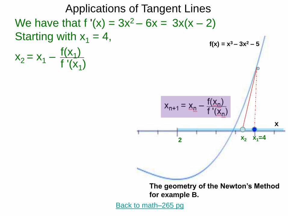
Applications of Tangent Lines
x2 = x1 – f(x1)f '(x1)
We have that f '(x) = 3x2 – 6x = 3x(x – 2)
Starting with x1 = 4,
x1=42
x
f(x) = x3 – 3x2 – 5
The geometry of the Newton’s Method
for example B.
Back to math–265 pg
x2
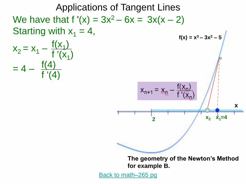
Applications of Tangent Lines
x2 = x1 – f(x1)f '(x1)
We have that f '(x) = 3x2 – 6x = 3x(x – 2)
Starting with x1 = 4,
= 4 – f(4)f '(4)
x1=42
x
f(x) = x3 – 3x2 – 5
The geometry of the Newton’s Method
for example B.
Back to math–265 pg
x2
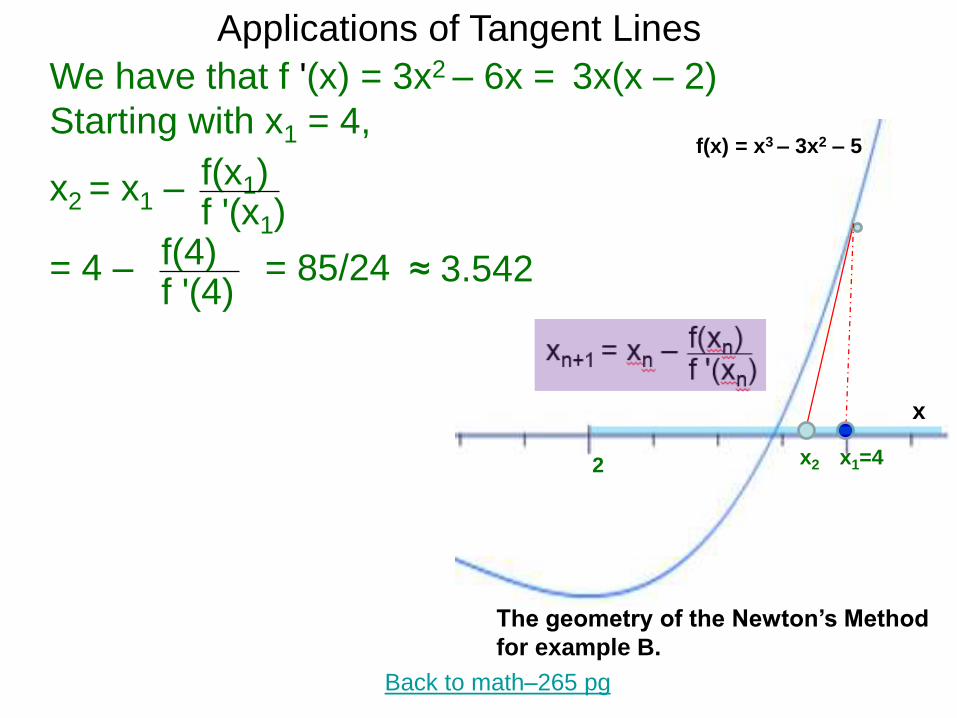
Applications of Tangent Lines
x2 = x1 – f(x1)f '(x1)
We have that f '(x) = 3x2 – 6x = 3x(x – 2)
Starting with x1 = 4,
= 4 – f(4)f '(4)
= 85/24
x1=42
x
f(x) = x3 – 3x2 – 5
≈ 3.542
The geometry of the Newton’s Method
for example B.
Back to math–265 pg
x2

Applications of Tangent Lines
x2 = x1 – f(x1)f '(x1)
We have that f '(x) = 3x2 – 6x = 3x(x – 2)
Starting with x1 = 4,
= 4 – f(4)f '(4)
= 85/24
x3 = 85/24 –f(85/24)f '(85/24)
x1=42
x
f(x) = x3 – 3x2 – 5
≈ 3.542
x3 x2
The geometry of the Newton’s Method
for example B.
Back to math–265 pg

Applications of Tangent Lines
x2 = x1 – f(x1)f '(x1)
We have that f '(x) = 3x2 – 6x = 3x(x – 2)
Starting with x1 = 4,
= 4 – f(4)f '(4)
= 85/24
x3 = 85/24 –f(85/24)f '(85/24)
≈ 3.432x1=42
x
f(x) = x3 – 3x2 – 5
≈ 3.542
x3 x2
The geometry of the Newton’s Method
for example B.
Back to math–265 pg
Applications of Tangent Lines
x2 = x1 – f(x1)f '(x1)
We have that f '(x) = 3x2 – 6x = 3x(x – 2)
Starting with x1 = 4,
= 4 – f(4)f '(4)
= 85/24
x3 = 85/24 –f(85/24)f '(85/24)
≈ 3.432x1=42
x
f(x) = x3 – 3x2 – 5
≈ 3.542
x3 x2The software answer is
≈ 3.425988..
The geometry of the Newton’s Method
for example B.
Back to math–265 pg