39 error detector placement for soft computing...

39

Error Detector Placement for Soft Computing Applications

ANNA THOMAS, University of British ColumbiaKARTHIK PATTABIRAMAN, University of British Columbia

The scaling of Silicon devices has exacerbated the unreliability of modern computer systems, and powerconstraints have necessitated the involvement of software in hardware error detection. At the same time,emerging workloads in the form of soft computing applications, (e.g., multimedia applications) can toleratemost hardware errors as long as the erroneous outputs do not deviate significantly from error-free outcomes.We term outcomes that deviate significantly from the error-free outcomes as Egregious Data Corruptions(EDCs).

In this study, we propose a technique to place detectors for selectively detecting EDC causing errors in anapplication. We performed an initial study to formulate heuristics that identify EDC causing data. Basedon these heuristics, we developed an algorithm that identifies program locations for placing high coveragedetectors for EDCs using static analysis. Our technique achieves an average EDC coverage of 82%, underperformance overheads of 10%, while detecting 10% of the Non-EDC and benign faults. We also evaluatethe error resilience of these applications under the fourteen compiler optimizations.

ACM Reference Format:Anna Thomas and Karthik Pattabiraman, 2014. Error Detector Placement for Soft Computing Applications.ACM Trans. Embedd. Comput. Syst. 9, 4, Article 39 (March 2010), 25 pages.DOI:http://dx.doi.org/10.1145/0000000.0000000

1. INTRODUCTIONWith the reduction of chip sizes and the concomitant increase in the number of transis-tors on a chip, the frequency of hardware faults is on the rise. Traditionally, hardwareerrors have been tolerated through hardware redundancy or guard banding. Unfortu-nately, hardware-only solutions have high energy overheads, and are challenging aspower becomes a dominant concern in processor design [Carter et al. 2010].

Recently, there have been several proposals to selectively expose hardware faultsto the software layer and tolerate them [Carbin and Rinard 2010; De Kruijf et al.2010; Leem et al. 2010; Liu et al. 2011; Narayanan et al. 2010]. These proposals lever-age the ability of certain software applications to tolerate faults in their data, andstill produce acceptable outputs. Such applications are called soft computing applica-tions [Zadeh 1997]. Soft computing applications have gained increasing prominence,and researchers have predicted that future workloads will belong primarily to thiscategory [Dubey 2005].

Examples of soft computing applications are multimedia decoding applications,which can tolerate blurry decoded images, and machine learning applications, whichcan tolerate noise. These applications have an associated fidelity metric, which is aquantitative measure of the output quality. For example, in the case of image and videodecoders, the fidelity metric is peak signal-to-noise ratio (PSNR). As long as the pro-

Author’s addresses: A. Thomas, (Current address) IBM , Toronto, CanadaK. Pattabiraman, Department of Electrical and Computer Engineering, UBC, Vancouver, CanadaPermission to make digital or hard copies of part or all of this work for personal or classroom use is grantedwithout fee provided that copies are not made or distributed for profit or commercial advantage and thatcopies show this notice on the first page or initial screen of a display along with the full citation. Copyrightsfor components of this work owned by others than ACM must be honored. Abstracting with credit is per-mitted. To copy otherwise, to republish, to post on servers, to redistribute to lists, or to use any componentof this work in other works requires prior specific permission and/or a fee. Permissions may be requestedfrom Publications Dept., ACM, Inc., 2 Penn Plaza, Suite 701, New York, NY 10121-0701 USA, fax +1 (212)869-0481, or [email protected].© 2010 ACM 1539-9087/2010/03-ART39 $15.00DOI:http://dx.doi.org/10.1145/0000000.0000000

ACM Transactions on Embedded Computing Systems, Vol. 9, No. 4, Article 39, Publication date: March 2010.

39:2 A. Thomas et al.

duced output quality does not deviate significantly from the fidelity metric, it is deemedacceptable. We use the term Egregious Data Corruptions (EDCs) to denote outcomesthat deviate significantly from the fidelity metric, i.e., unacceptable outcomes.

The error tolerance of soft computing applications does not mean that they are re-silient to all errors. In particular, an error in a soft computing application may or maynot lead to an EDC. If it will lead to an EDC, then the application needs to be stopped,as otherwise, its output will be unacceptable. On the other hand, if the error will notlead to an EDC, it is better to let the application continue rather than perform wastefuldetection and recovery, and incur unnecessary overheads. This overhead will becomemore prominent as error rates increase, as they are predicted to in future processors.

Our goal is to efficiently place error detectors in soft-computing applications in orderto detect errors early (thus avoiding egregious outcomes), at the same detecting onlythose errors that lead to EDCs (thus avoiding wasteful recovery). An error detectoris an assertion or check on one or more data variables in the application. We developheuristics that determine where to place error detectors for avoiding EDCs, using faultinjection and static analysis of the application’s code. While we use fault injection todevelop the heuristics, we do not require fault injection to apply the developed heuris-tics to new applications. This is because our heuristics are based on static and dynamicproperties of the application’s code, and do not rely on semantic knowledge of the ap-plication. Note that fault-injection is a time intensive process for large applications,and hence it is desirable to avoid it (if possible).

Prior work [Hiller et al. 2002; Leeke et al. 2011; Pattabiraman et al. 2005] has in-vestigated the problem of optimal error detector placement. However, these techniquesfocus on placing detectors to minimize the error detection latency or to detect specificfailures such as safety violations. In particular, they do not consider optimizing the de-tector placement for minimizing the EDC rate, which is important for soft computingapplications. As we show later, minimizing the EDC rate leads us to different place-ment decisions than if we had optimized for minimizing the number of Silent DataCorruptions (SDCs), which constitute any deviation from the correct output (not onlyegregious ones) [Hari et al. 2012].

Recent work [Baek and Chilimbi 2010; Carbin et al. 2013; Samadi et al. 2013; Samp-son et al. 2011] focus on approximate computing where accuracy of results is tradedfor performance benefits or lower energy consumption, by developing architectural ortype-based solutions. For example, [Samadi et al. 2013] modifies the application codeto generate approximate kernels to run on GPUs. Our work is also on similar applica-tions which do not require precise results, but we study these applications from a faulttolerance and reliability perspective, through static analysis and execution profile.

We make the following contributions in this work:

(1) We perform fault injection into soft computing applications, and distinguish EDCsfrom the set of SDCs. Based on the injections, we develop heuristics for identifyingEDC-prone regions of code or data, which are appropriate candidates for detectorplacement.

(2) We develop a systematic algorithm based on these heuristics, that (a) ranks the dataaccording to their EDC causing nature, based on static analysis (b) uses a greedyapproach that combines the static information, with the dynamic execution profile,to choose the appropriate set of EDC data or code for placing detectors. Our algo-rithm takes as input the application source code, the acceptable performance over-head, and the execution profile data of the application, and identifies the locationsto place detectors in the program, i.e., data or instructions.

(3) We implement the algorithm within the LLVM compiler, and evaluate its accuracythrough fault-injection. We find that the detectors placed by the algorithm provide


Error Detector Placement for Soft Computing Applications 39:3

Fig. 1: The EDC causing fault decoded image (left) versus Non-EDC causing fault decoded image(right) from the JPEG decoder

EDC coverage of 82% under 10% performance overhead, while providing a Non-EDCand benign coverage of only 10%.

(4) We study the effect of individual compiler optimizations on the error resilience andvulnerability of soft computing applications, both with and without our technique.While compiler optimizations may enhance application performance, they mightlower the application error resilience. We also identify safe optimizations, or thosethat do not affect the error resilience significantly, when detectors are placed in theapplication.

2. BACKGROUNDEgregious Data Corruption (EDC) is a relative term as it depends on how the usersets the fidelity threshold. In this paper, we focus on detecting errors under the as-sumption that the user tolerates most small deviations in outputs, i.e., the applicationis used under relaxed conditions. For example, in image and video decoding applica-tions, we set the fidelity threshold based on whether the frames are corrupted to thepoint of being unrecognizable or are of very poor image quality. In other cases, wherewe cannot rely on human perception, we set the fidelity threshold to be such thataround 30% of the most egregious SDCs are categorized as EDCs (see Section 5).

The example in figure 1 shows the faulty decoded images of the MediaBench JPEGdecoder [Lee et al. 1997], when a fault is injected into the program. The fidelity thresh-old is Peak Signal to Noise Ratio (PSNR) between the fault-free decoded image, andthe faulty decoded image. As the PSNR value becomes lower, the output corruptionbecomes more egregious. Assuming a fidelity threshold value of PSNR 30, the faultyimage on the left with a PSNR of 11.37 is classified as an EDC, while the faulty imageon the right with a PSNR value of 44.79 is classified as a Non-EDC. The comparison isperformed with respect to the base image, which we do not show.

Challenge: Prior research has shown that faults in data constituting higher dy-namic execution time are more likely to cause SDCs [Hari et al. 2012]. In other words,SDC causing code tends to be on the hot paths of the application. However, EDCsare caused by a large deviation in output, and are not necessarily caused by faults indata on the hot paths. For example, consider function conv422to444 from the MPEGbenchmark in Mediabench (Figure 2 in Section 3), which converts from YUV 4:2:2 sub-sampling (U and V components are sampled at half the rate of Y component) to YUV4:4:4 (all components sampled at same rate). The longest running statements are thelines 8 to 11, the ones within two nested for loops. A fault at the branch i < 1 at B4,or at the pointer data P1, causes an SDC but not an EDC. However, a fault occurringat loop termination conditions B2 and B3 cause an EDC.

Therefore, to maximize the coverage for EDCs, detectors should be placed at coderegions or data that have the highest impact on the application’s output. The mainchallenge in detecting EDCs is coming up with a general algorithm to identify such



code or data. Further, the algorithm should be based only on the static code of theprogram and its execution profile, and not require fault injections, which are expensive.

Fault Model: We consider transient hardware faults that occur in the processor.These are usually caused by cosmic ray or alpha particle strikes affecting flip flops andlogic elements. We consider faults that occur in the functional units, i.e., the ALU andthe address computation for loads and stores. However, faults in the memory compo-nents such as caches are not considered, since these components are usually protectedat the architectural level using ECC or parity.

We focus on transient faults because they occur more frequently than permanenterrors [Siewiorek 1991]. Further, rates of transient errors are projected to increasesignificantly due to the effects of technology scaling [Shivakumar et al. 2002]. Extend-ing our fault model to permanent errors is a direction for future research.

Initial Study: To identify characteristics of EDC causing faults, we performed faultinjection experiments on six applications of MediaBench I and II [Fritts et al. 2005; Leeet al. 1997]. These are video/image decoders - JPEG, MPEG2 and H264Dec, and speechdecoders - G721, GSM and ADPCM. We use LLFI [Thomas and Pattabiraman 2013b],our program level fault injector that works at the LLVM compiler’s intermediate codelevel [Lattner and Adve 2004], to perform the experiments.

Using LLFI, we injected faults (single bit flips) into pointers and control data, andmonitored the fault propagation. The outcome of the fault was classified into Crash,EDC, Non-EDC and Benign, by comparing the final output with the fault free outcome.The fault-free or baseline outcome is obtained by running the original executable withthe same input, but without any injected faults. Crashes are classified as those causingabnormal program termination, whereas benign outcomes have no change from thefault-free outcome. We found that faults belonging to the backward slice of controland pointer data have a higher chance of causing EDCs (for example, faults in looptermination conditions)1.

3. HEURISTICSWe formulated heuristics to identify detector placement points for EDCs, on the basisof our initial study. All of these heuristics have the common characteristic of beingdependent on the size of the data being affected, either within the branches or indownstream computations. We unify these heuristics using a ranking expression inour algorithm explained in Section 4.

We explain the heuristics with the code in Figure 2 as a running example. This codeis based on the MPEG video decoding benchmark from the Mediabench benchmarksuite. However, for elucidation purposes, we have added extra code to these functions(we explain what these are later). The store ppm tga function stores the decoded imagein a ppm file. The Show Bits(N) function returns the next N bits of the image, withoutadvancing the pointer.

We divide the problem of formulating heuristics for identifying detector placementpoints into two steps. First, we identify functions in the program that are likely toresult in EDCs when affected by faults. Second, we identify statements (and variables)within a function at which detectors need to be placed in order to detect EDCs.

3.1. Step 1: Function IdentificationWe first identify program functions in which we need to place detectors, based onwhether the functions have side effects. A side-effect free function has the followingtwo characteristics, both of which must be satisfied:

1The fault injection methodology, examples and complete results are presented in detail in our priorwork [Thomas and Pattabiraman 2013b].



(1) Statements within these functions do not modify global variables, files and pointers,though they may read them.

(2) The functions have a return value and this is the only result of the function used byits caller function

1 void conv422to444 ( char *src , char* dst , int width , int height , int offset ){2 . . .3 w = width>>1;4 if(dst < src + offset) / / B15 return ;67 f or ( j=0; j < height ; j++) { / / B28 for ( i=0; i < width ; i++) { / / B39 i2 = i<<1;

10 im1 = (i < 1) ? 0 : i�1; / / B411 . . .12 dst [ i2 ] = Clip [ (21* src [ im1 ] )>>8]; / / P113 }14 if(j + 1 < height) { / / B515 src += w ; / / P216 dst += width ;17 }18 }19 . . .20 }21 void store_ppm_tga ( int width , int height ){22 int i , j , singlecode ;23 char *u444 [ NUMFRAMES ] ;24 int *code [ NUMFRAMES ] , codeframes [ NUMFRAMES ] ;25 . . .26 / / int * b i t l o cn [NUMFRAMES] i s global27 f or ( i=0; i < NUMFRAMES ; i++){ / / B628 for ( j=0; j < width ; j++)29 singlecode += Show_Bits ( bitlocn [ i ] [ j ] ) ; / / C030 codeframes [ i ] = singlecode ;31 }32 f or ( i=0; i < NUMFRAMES ; i++) / / B733 for ( j=0; j < width ; j++) / / B834 code [ i ] [ j ] = Show_Bits ( bitlocn [ i ] [ j ] ) ; / / C135 . . .36 singlecode = Show_Bits ( 8 ) ; / / C237 . . .38 / / char * source [ ] i s g lobal39 i f ( CHROMA_FORMAT == YUV422 ){ / / B940 for ( i=0; i < NUMFRAMES ; i++) / / B1041 conv422to444 ( source [ i ] , u444 [ i ] , width , height , offset ) ; / / C342 }43 . . .44 }45 main ( ) {46 . . .47 store_ppm_tga ( width , height ) ;48 . . .49 }50 unsigned int Show_Bits ( int N ){51 / / ld i s a global struct52 return ld�>Bfr >> (32�N ) ;53 }

Fig. 2: Example Code for Function and Data Categorization

We call such functions Optimized EDC Functions (OEF). For example in Figure 2,Show Bits() is an OEF, as it satisfies the conditions outlined above. Once an OEFcall is identified as EDC-causing, it suffices to place a detector at the return value of



the particular call. No other detectors are required for the OEF, and hence the nameOptimized EDC. We find that EDCs are caused by only certain calls to OEFs, and weformulate a heuristic for identifying such OEF calls.

H1: The likelihood of an EDC due to a fault in an OEF increases as the amount ofdata affected by its return value increases.

By the definition of OEFs, the data modified within these functions is local to thefunction. Therefore, the data modified by an OEF call is dependent on the propagationof the function’s return value. For example, Show Bits(), which is an OEF, is called atthree places in the code, namely C0, C1 and C2. When a fault occurs in the OEF, thereturn value of the function call at C1 affects only one element of the 2D code array.This fault does not cause an EDC. On the other hand, the function call in C0 is a loopcarried dependency, and the singlecode variable is assigned to the elements of arraycodeframes in the outer loop. The return value from the C0 call thus influences a largeramount of data than the return value from call C1. Therefore, we will place a detectoron the return value in call C0, but not on the return value in call C1.

Note that this heuristic only applies to OEFs called within loops. When the OEFis not called within a loop, we do not place any detector at the return value. Thisis because such faults usually cause an EDC when they propagate to branches, andwould be caught by detectors at those branches.

The remaining functions are side-effect causing functions which do not satisfy con-ditions for OEFs (conv422to444 and store ppm tga). We elaborate the heuristics appli-cable to such functions in the following section.

3.2. Step 2: Data CategorizationWithin functions that are not OEFs, we found that faults affecting certain control andpointer data are highly likely to cause EDCs.

Control Data: Control data can be divided into loop or function terminating branchconditions, and other branches, i.e., those that do not terminate loops or functions.For example, B1 is a function terminating branch, while j < height at B2 is a loopterminating branch. The heuristics are based on faults that either directly affect orpropagate to these branches, and cause the branch to flip.2

H2. The EDC causing nature of the loop terminating conditions decreases, as we godeeper within nested loops. This is because the amount of data modified by outer loopsis much larger than the data modified by inner loops. For example, a fault at branchcondition i < NUMFRAMES at B7 has a higher likelihood of causing an EDC than one atbranch condition j < width at B8, as it affects more elements of the array code.

H3. The likelihood of an EDC due to faults at function terminating conditions in-creases as the amount of data affected in downstream computations within that func-tion increases, and as the inter-procedural loop nesting level decreases.

The EDC causing nature of function terminating branches increases, as the amountof data affected downstream within that function increases. For example, a fault atB1, causing a branch flip to true, abnormally terminates function execution, therebymissing the loop computations at B2. Also, the function terminating branch B1 has aloop level of 1, since the function conv422to444 is called within a loop at C3. Thesetwo factors, i.e., the downstream loop computations and the low loop nesting level,contribute to a high likelihood of an EDC, when the fault occurs or propagates to B1.

H4. Branch conditions that do not terminate functions or loops are likely to causeEDCs if and only if the amount of data affected within the body of the branch is large.

2In our initial study, we found that faults causing branch flips are much more predominant than those thatdo not cause a flip for control data.



(1) When the branch body consists of assignments to pointers, or several elements of anarray or aggregate structure, a fault occurring at the branch results in an EDC. Inthe above example, we place a detector after branch B5 since the body of the branchchanges the pointers src and dst.

(2) When the branch body consists only of a change to a single element of an array, orsome local variable, a fault in the branch results in an SDC, but not an EDC. Forexample, the ternary condition i < 1 at B4 is a Non-EDC causing branch, since itonly changes the index of one element in the array src, thereby corrupting the valueof one element of array dst.

(3) When a branch condition (that does not terminate loops or functions) has loopswithin it, a fault at the branch condition has a high likelihood of causing an EDC.This is because the amount of data modified is large in the loop body. For example,a fault causing a branch flip at B9 has a high likelihood of causing an EDC, since itcauses the loop at B10 to be skipped, thereby affecting the computation of the entirearray u444.

Pointer Data: Examples are pointer dereferences, accesses to specific elementswithin aggregate structures, and pointer assignments or arithmetic. Our fault injec-tion experiments (in Section 2) show that the number of faults leading to crashes,SDCs and EDCs are high for pointer data that do not cause any control deviation.This pointer data usually occurs within loop bodies. As prior work finds [Hari et al.2012], crashes are caused when a bit flip occurs in the high order bits of the memoryaccess, whereas SDCs are caused when the bit flip is in the low order bits. However,we find that some pointer address computations are more likely to cause an EDC, andwe formulate a heuristic to identify these computations.

H5. Faults in the low order bits of pointers pointing to larger sized data have higherlikelihood of causing an EDC. For example, faults in the low order bits of pointer datafor src at P2 causes an EDC. However, a fault at the lower bits of the Clip, src or dstarray indices at P1 causes an SDC, but not an EDC.

4. APPROACHIn this section, we first present the usage model for our technique, and then discuss ouralgorithms to identify program locations for high coverage detectors for EDC causingerrors. These are based on the heuristics we developed in Section 3.

Fig. 3: Technique Workflow with required inputs

Usage Model: The goal of our technique is to preemptively detect EDC causingfaults in soft computing applications, under a given performance overhead that theuser is willing to tolerate. The technique requires as inputs from the user: (a) theapplication source code, (b) the maximum permissible performance overhead, and (c)the application’s execution profile, under representative inputs.



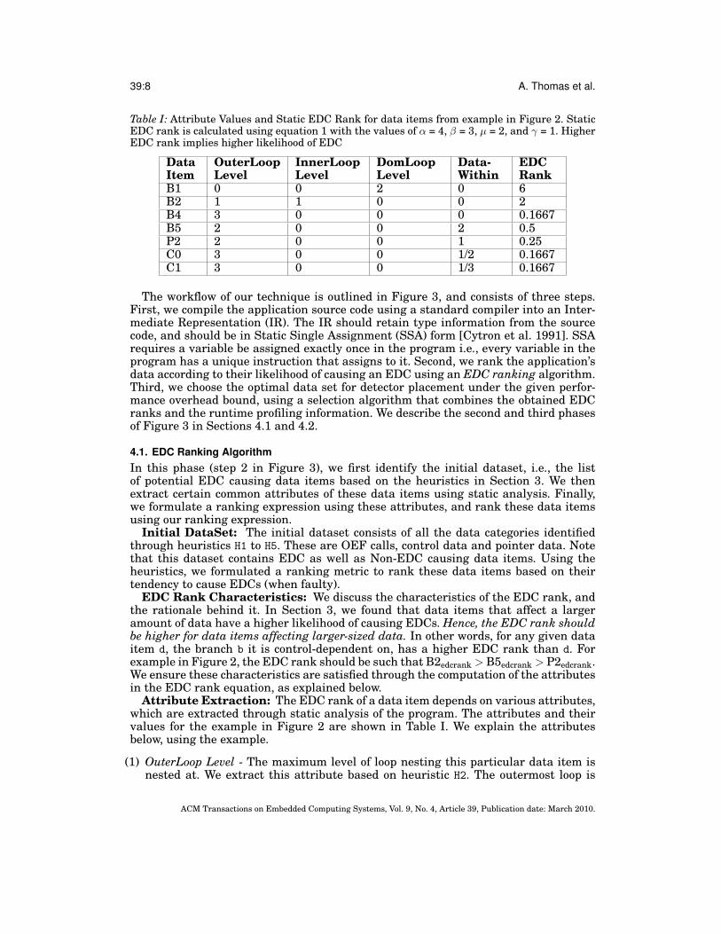
Table I: Attribute Values and Static EDC Rank for data items from example in Figure 2. StaticEDC rank is calculated using equation 1 with the values of ↵ = 4, � = 3, µ = 2, and � = 1. HigherEDC rank implies higher likelihood of EDC

DataItem

OuterLoopLevel

InnerLoopLevel

DomLoopLevel

Data-Within

EDCRank

B1 0 0 2 0 6B2 1 1 0 0 2B4 3 0 0 0 0.1667B5 2 0 0 2 0.5P2 2 0 0 1 0.25C0 3 0 0 1/2 0.1667C1 3 0 0 1/3 0.1667

The workflow of our technique is outlined in Figure 3, and consists of three steps.First, we compile the application source code using a standard compiler into an Inter-mediate Representation (IR). The IR should retain type information from the sourcecode, and should be in Static Single Assignment (SSA) form [Cytron et al. 1991]. SSArequires a variable be assigned exactly once in the program i.e., every variable in theprogram has a unique instruction that assigns to it. Second, we rank the application’sdata according to their likelihood of causing an EDC using an EDC ranking algorithm.Third, we choose the optimal data set for detector placement under the given perfor-mance overhead bound, using a selection algorithm that combines the obtained EDCranks and the runtime profiling information. We describe the second and third phasesof Figure 3 in Sections 4.1 and 4.2.

4.1. EDC Ranking AlgorithmIn this phase (step 2 in Figure 3), we first identify the initial dataset, i.e., the listof potential EDC causing data items based on the heuristics in Section 3. We thenextract certain common attributes of these data items using static analysis. Finally,we formulate a ranking expression using these attributes, and rank these data itemsusing our ranking expression.

Initial DataSet: The initial dataset consists of all the data categories identifiedthrough heuristics H1 to H5. These are OEF calls, control data and pointer data. Notethat this dataset contains EDC as well as Non-EDC causing data items. Using theheuristics, we formulated a ranking metric to rank these data items based on theirtendency to cause EDCs (when faulty).

EDC Rank Characteristics: We discuss the characteristics of the EDC rank, andthe rationale behind it. In Section 3, we found that data items that affect a largeramount of data have a higher likelihood of causing EDCs. Hence, the EDC rank shouldbe higher for data items affecting larger-sized data. In other words, for any given dataitem d, the branch b it is control-dependent on, has a higher EDC rank than d. Forexample in Figure 2, the EDC rank should be such that B2edcrank > B5edcrank > P2edcrank.We ensure these characteristics are satisfied through the computation of the attributesin the EDC rank equation, as explained below.

Attribute Extraction: The EDC rank of a data item depends on various attributes,which are extracted through static analysis of the program. The attributes and theirvalues for the example in Figure 2 are shown in Table I. We explain the attributesbelow, using the example.

(1) OuterLoop Level - The maximum level of loop nesting this particular data item isnested at. We extract this attribute based on heuristic H2. The outermost loop is



at level 1, the next loop at level 2, and so on. For data items that are not loopor function terminating, the loop level is one level more than the number of loopsit is nested within. This is to satisfy the EDC rank characteristic, and unify theattribute extraction across all data items. For example, branch B4 in Table I hasouterloop level of 3.

(2) InnerLoop Level - The maximum level of loop nesting within this data item. Weextract this attribute based on heuristics H2 and H4. For example, branch B2 has aninnerloop level of 1.

(3) DomLoop Level - The maximum level of loop nesting dominated by this particulardata item, but excluding the innerloop level. The data item d dominates a loop ifevery path in the control flow graph from the start node to the loop should pass d. Weextract this attribute based on heuristic H3. For example, the function terminatingcondition B1 has value 2 in Table I.

(4) DataWithin - The amount of data affected by the data item. This applies to OEFcalls, branches that are not loop or function terminating, and pointer data. We ex-tract this attribute based on heuristics H1, H4 and H5. For pointer assignments andarithmetic, the numerical value of datasize is equal to the level of pointer indirec-tion. In case of array accesses, the datasize is computed as 1/(1 + number of arrayindices). For example, the datasize for both pointer data P2, and OEF calls C0 andC1 is shown in Table I.Static EDC Rank Expression: The EDC rank of a data item is the likelihood of

an EDC outcome, given that a fault occurs at the data item or propagates to it. Weformulate the rank expression using the attributes identified before:

max(↵ ⇤ InnerLoop+ � ⇤DomLoop+ � ⇤DataWithin, 1)max(µ ⇤OuterLoop, 1)

(1)

where ↵, �, � and µ are parameters quantifying the importance of the respective at-tributes, i.e., InnerLoop level, DomLoop level, DataWithin and OuterLoop level. Toavoid zero values in the numerator and denominator, we assign the minimum value tobe 1 in both parts. We followed an educated trial and error method to assign the valuesfor ↵, �, � and µ. The values assigned are ↵ = 4, � = 3, � = 1 and µ = 2. We explain theassignment of these values in our prior work [Thomas and Pattabiraman 2013a].

4.2. Selection AlgorithmIn this phase, i.e., step 3 in Figure 3, we identify the optimal set of locations to place de-tectors in the program based on the EDC rank (from the previous phase), the allowedperformance overhead and execution profile of the application. We use the profile datato maintain the bound on the performance overhead specified by the user, while ac-counting for the likelihood of a fault affecting the data item. We obtain the profiledata by running the application with representative inputs provided by the user (seeSection 5).

We model the problem of selecting the EDC data items as the 0-1 knapsack prob-lem [Cormen et al. 2001]. Each EDC data item d has an associated weighted EDC rankdwrank (the objective function we maximize) and a performance overhead dpo, measuredas the number of extra instructions that would need to be executed if the element isselected. Our goal is to select the items to put into the knapsack to maximize the ranksubject to a given performance overhead. The weighted EDC rank is calculated usingthe following equation:

dwrank = (norm(dedcrank) + 1)/F funcrank (2)where F is the function containing the data item d. The normalization function norm,converts the edcrank (obtained from previous phase) to a value between 0 and 1. The



funcrank is the rank of the function in descending order of their execution time. Wechoose the set of detector locations (the knapsack), using the following criteria

maximize(⌃dwrank) such that ⌃(dpo) P (3)

where P is the user specified maximum performance overhead.A naive approach to solving the knapsack problem is a greedy one of choosing the

item with the maximum weighted rank that satisfies the performance overhead con-straint. However, a naive greedy algorithm may make a sub-optimal decision in choos-ing data items as it does not have a lookahead capability. We use a variant of the greedyalgorithm that has a parameter controlling the function rank, and a lookahead win-dow to avoid making a short-sighted, sub-optimal decision. We explain the algorithmusing an example. Let us consider five functions A, B, C, D and E, whose executiontimes are 10, 8, 6, 4 and 1 milli-seconds, respectively. If we used a naive greedy al-gorithm, then the funcrank would be simply incremented as function execution timesdecreased. In this case, A, B, C, D and E would have respective funcranks of 1, 2, 3, 4and 5. The selection algorithm would start filling the knapsack with data items of Ain descending order of edcrank, followed by that of B, and so on, until the maximumperformance overhead P is reached. Hence, the Non-EDC data in function A will getincluded, and we may miss the EDC data in the remaining functions, leading to asub-optimal solution.

To overcome this problem, we use a funcrange parameter to increment the func-tion rank. All functions having execution times within the funcrange have the samefunction rank. We also use a lookahead window with functions having the next higherfunction rank. Assuming funcrange with value 2, then functions A, B and C have afunction rank of 1, D has a rank of 2, and E has a rank of 3. We explain how theseranks are obtained in algorithm in Figure 4. The selection window has functions A, Band C, while the lookahead window contains function D. Now, the knapsack is filledin descending order of dwrank (where d is data items of A, B, C and D) until all thedata items in the selection window are added. Next, the selection window slides aheadto D, and the lookahead window slides to E. The same process of filling the knapsackand sliding the window is repeated, until P is reached. As the funcrange parameterincreases, more functions would have the same function rank. Hence, the choice of de-tector locations would be based on a larger set of data, and hence be more optimal thana naive greedy algorithm.

The algorithm to calculate the weighted EDC rank using funcrange of N is presentedin Figure 4. It considers the functions in the program in decreasing order of their ex-ecution times. All functions within the funcrange have the same function rank. Whena function whose execution time is outside the parameter is encountered, the functionrank is incremented. If a function is an OEF, it is skipped (see Section 4.1). After cal-culating the weighted EDC ranks for all the data items, the final set of EDC detectorlocations is computed using equation 3.

5. EXPERIMENTAL SETUPIn this section, we present the implementation details of our technique, followed bythe benchmarks, the fidelity thresholds and the evaluation metrics.

Implementation: We implemented the EDC ranking and the selection algorithm(steps 2 and 3 in Figure 3) as custom passes in the LLVM compiler version 2.9. First,the application source code is compiled into LLVM Intermediate Representation (IR)along with the mem2reg optimization (i.e., promote loads/stores to registers). Second,the IR is statically (a) analyzed to compute the static EDC rank for the EDC dataset,



1 f l o a t funcrank = 1;2 int funcrange = N ;3 map funcrankmap ;4 map EDCrankmap ;5 int main ( ) {6 map weightedrankmap ;7 function topFunc = Function with max exec time ;8 f o r each function 'F ' ranked in decreasing order of execution times{9 i f ( F is an OEF )

10 continue ;11 i f ( topFunc . exectime / F . exectime > funcrange ){12 funcrank++;13 topFunc = F ;14 }15 funcrankmap [ F ] = funcrank ;16 }1718 f or each dataitem ' d ' in initial DataSet{19 f l o a t weightedrank = calculateweightedrank ( d ) ;20 weightedrankmap [ d ] = weightedrank ;21 }22 }2324 f l o a t calculateweightedrank ( dataitem d ){25 Function F = d . getFunction ( ) ;26 return ( ( norm ( EDCrankmap [ d ] ) +1) / funcrankmap [ F ] ) ;27 }

Fig. 4: Pseudo-code to show the calculation of weighted rank using funcrange = ’N’ where ED-Crankmap is map of static EDC ranks for all data items using equation 1

and (b) instrumented to place detectors identified using profile data3 under the givenperformance overhead bound. Third, the instrumented IR is compiled into machinecode using the LLVM compiler.

We used funcrange of 5 in our experiments based on coverage results obtained byvarying its value (see [Thomas and Pattabiraman 2013a] for details). The time re-quired for our custom passes, is on average less than three seconds across the bench-marks. The error detectors are derived by replicating the static inter-procedural back-ward slice of the EDC data item, and placing a comparison statement after the copyof the item. We simulate our detectors by instrumenting the IR with trace calls atthe locations chosen for detector placement. These trace calls record the values of theEDC data in a file, and a fault is detected if the fault-free and faulty trace files differ.The fault-free trace file is obtained by running the instrumented program on the sameinput, with no faults injected.

We measure the performance overhead of our detectors as the dynamic executionoverhead of the extra code added (replicated code and comparison statements). Weassume that faults do not affect detectors, and hence we do not inject faults into them.This is because we assume that only one fault occurs in each run of the applicationand a fault in the detector does not affect EDC coverage, as the worst outcome of sucha fault is that it stops the program, and does not cause an EDC.

We simulate ideal detectors, as we do not consider reaching stores for loads, andfunction pointers when computing the backward slice. Hence, the coverage may belower with actual detectors based on this backward slice. Also, since we approximatethe backward slice, the performance overhead does not reflect the actual overhead of

3We wrote a custom pass for obtaining profile data and for measuring the performance overhead, usingLLVM basic block profiling pass.



these ideal detectors. We compare the coverage results of the actual detectors underthe actual performance overhead, versus our ideal detectors in Section 6.2.

Table II: Characteristics of Benchmark Programs. Higher distortion (scaled difference) is moreegregious, lower PSNR is more egregious.

Benchmark(Lines ofC/C++ Code)

Description Input Fidelity Metric (thresholdvalue)

BlackScholes(1661)

Compute option pricingusing Black-Scholes PartialDifferential Equation

Sim-large Scaled difference of optionprices (0.3)

X264 (37454) Media Application perform-ing H.264 encoding of video

test Mean distortion of PSNR (asmeasured by H.264 referencedecoder) and the encodedvideo’s bitrate (0.017)

Canneal(4506)

Simulated cache-aware an-nealing to optimize routingcost of a chip design

Sim-dev Scaled difference of routingcost between faulty and origi-nal version (0.026)

Swaptions(1428)

Price portfolio of swaptionsusing Monte Carlo Simula-tions

Sim-small Scaled difference of swaptionprices (0.00001)

JPEG(30579)

Image Decoder test-img.jpg

PSNR between faulty andfault-free decoded images(30)

MPEG2(9832)

Video Decoder mei-16v2.m2v

PSNR between faulty andfault-free decoded image set(30)

Benchmarks: We use four applications from Parsec [Bienia et al. 2008], and twofrom Mediabench [Lee et al. 1997] for evaluating our technique. These are a mix offinancial, multimedia and VLSI CAD applications, and have been used as soft comput-ing applications in prior work [Cong and Gururaj 2011; Li and Yeung 2007; Misailovicet al. 2010; Sundaram et al. 2008]. The benchmark characteristics are explained inTable II.

For the profile data, we need the user to provide representative inputs. However, theinputs are only used for calculating the performance overhead and the function rank.We have verified that the variation in EDC coverage is minimal across the providedinputs for these benchmarks, compared to the inputs in Table II. We observed a 3%variation in EDC coverage for JPEG with input lena.jpg. We observed less than 2%difference in coverage for BlackScholes, Swaptions and X264. The inputs used weresim-dev, sim-medium, and eledream 64x36 3.y4m respectively. We did not have otherinputs for MPEG and Canneal.

The majority of the programs are different from what we chose in our initial study, inwhich we only use Mediabench. We use only two programs from Mediabench (MPEGand JPEG) out of the six from our initial study. We do not use G721 and GSM, becausetheir fidelity metric values show very slight variation, making it difficult to separatethe EDCs from Non-EDCs, even manually. ADPCM is a small benchmark programwith 740 lines of code, while H264Dec overlaps significantly with the Parsec bench-mark X264, and hence both are skipped. The other four programs are from the Parsecsuite. We made small changes to Blackscholes, Canneal and Swaptions benchmarkprograms as explained in our prior work [Thomas and Pattabiraman 2013a].

Fidelity Metrics and Threshold Values: We use the QoS metrics from priorwork [Misailovic et al. 2010] as the fidelity metrics for the Parsec benchmarks. We



distinguish EDCs from Non-EDCs using the fidelity threshold value (mentioned inparantheses in column 4 of Table II). This threshold value does not change betweeninputs. The distortion or scaled difference is the difference in absolute values betweenfaulty and original fault-free value divided by the original fault-free value. For theParsec benchmarks, we chose the fidelity threshold value such that 30% of the mostegregious deviations from the SDC set are classified as EDCs. For MPEG and JPEG,we performed manual inspection of all the faulty outputs, and we noticed that EDCswere caused when the PSNR value was below 30, i.e., the images were severely dis-torted. Hence, we choose the value 30 as the fidelity threshold for these two programs.

Coverage Evaluation: We evaluate our technique by performing fault injection onthe benchmark programs in Table II. We use our LLVM compiler based fault injectorLLFI to perform the injections, and classify the outcomes as Crash, Benign, EDC andNon-EDC as explained in Section 2. The applications are run using the LLVM Just-In-Time (JIT) compiler with the default optimization level of O2. We injected 2000 faultsper benchmark. The EDC rates are statistically significant within an error bar of 1.32%at the 95% confidence interval.

We inject only one fault in each run, as we assume that transient faults are relativelyrare events compared to the total execution time of an application. All injected faultsare executed i.e., the instruction into which the fault was injected is executed by theprogram.

We measure the coverage under varying bounds on performance overheads, i.e., 10%,20% and 25% (provided by the user) 4. The EDC coverage is the fraction of detectedEDCs out of total EDCs, while the Non-EDC and benign coverage is the fraction ofdetected Non-EDCs and Benign faults out of the total Non-EDC and Benign faults. Wedo not consider crashes as they are easily detected by program termination.

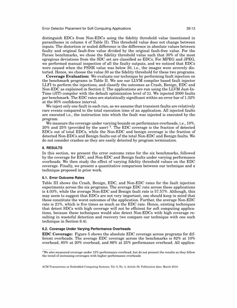
6. RESULTSIn this section, we present the error outcome rates for the six benchmarks, followedby the coverage for EDC, and Non-EDC and Benign faults under varying performanceoverheads. We then study the effect of varying fidelity threshold values on the EDCcoverage. Finally, we present a quantitative comparison between our technique and atechnique proposed in prior work.

6.1. Error Outcome RatesTable III shows the Crash, Benign, EDC, and Non-EDC rates for the fault injectionexperiments across the six programs. The average EDC rate across these applicationsis 4.03%, while the average Non-EDC and Benign fault rate is 57.57%. Although, thismay seem to suggest that EDCs are not very important, one should keep in mind thatthese constitute the worst outcomes of the application. Further, the average Non-EDCrate is 21%, which is five times as much as the EDC rate. Hence, existing techniquesthat detect SDCs with high coverage will not be efficient for soft computing applica-tions, because these techniques would also detect Non-EDCs with high coverage re-sulting in wasteful detection and recovery (we compare our technique with one suchtechnique in Section 6.4).

6.2. Coverage Under Varying Performance OverheadsEDC Coverage: Figure 5 shows the absolute EDC coverage across programs for dif-ferent overheads. The average EDC coverage across the benchmarks is 82% at 10%overhead, 85% at 20% overhead, and 86% at 25% performance overhead. All applica-

4We also measured coverage under 15% performance overhead, but do not present the results as they followthe trend of increasing coverages with higher performance overheads



Table III: Percentage of Error outcomes in each benchmark

Benchmark Crash (%) Benign (%) EDC (%) Non-EDC (%)BlackScholes 51.52 13.25 10 25.23X264 28.4 64.9 2.72 4.53Canneal 53.25 37.87 2.9 5.98Swaptions 42.05 48.46 2.57 6.92JPEG 29.27 30.38 4.03 36.27MPEG2 25.85 22.83 2.01 49.37Average 38.39 36.19 4.03 21.38

tions except for Swaptions, have an EDC coverage of 80-100% (average being 96%) at25% overhead. Hence, our technique detects EDCs with high coverage (above 80%) infive out of six applications, with low overheads (10%).

Fig. 5: EDC Coverage using our technique under performance overheads of 10%, 20% and 25%.Higher is better.

The lowest EDC coverage of our technique is for the Swaptions program (45%). It isinteresting to note that Swaptions has a relatively low EDC rate of 2.5%. On furtherinvestigation, we found that many EDCs are caused by faults in the uniform randomnumber generator function RanUnif(). The values returned by RanUnif are used in therest of Swaptions as an input for Monte-Carlo simulations. However, this location isnot chosen by our detector placement algorithm under the given performance overheadbounds. Our technique protects this function call only at 35% performance overheadbound, at which point the coverage increases to 80%. We believe this is an anomalouscase as we do not see this behaviour in any of the other five benchmarks.

Since we use simulated ideal detectors for our experiments (Section 5), we studythe EDC coverage of the actual detectors under the performance overhead of 25%.The results show that Blackscholes, Swaptions and Canneal have the same coverageas our simulated detectors, with an average EDC coverage of 71% versus 72% withthe ideal detectors. The remaining three benchmarks MPEG, JPEG and X264, have acoverage drop to an average of 56% because of the faults propagating to loads whichinitially occurred at backward slice of one of their reaching stores (flush buffer functionin MPEG and x264 cabac encode decision c in X264). This can be partially resolvedthrough a more accurate pointer analysis, which our current infrastructure does notsupport. However, this is not a fundamental limitation of our approach.

Non-EDC and Benign Coverage: Figure 6 shows the Non-EDC and Benign cov-erage using our technique. Lower coverage is better as benign and Non-EDC faults



are tolerated by the user, and we perform wasteful recomputation if these faults aredetected as EDCs and recovered from. The average coverage is 10%, 16% and 17.6%under respective performance overheads of 10%, 20% and 25%. Further, the averagebenign fault coverage is lower than the Non-EDC coverage.

Fig. 6: Non-EDC and Benign Coverage for our technique, under performance overheads of 10%,20% and 25%. Lower is better.

Summary: From Figures 5 and 6, one can observe that under 10% performanceoverhead, the average EDC coverage is 82%, while the Non-EDC and Benign coverageis about 10%. When the performance overhead is increased to 25%, the average EDCcoverage is 86%, while the Non-EDC and Benign coverage is 18%. Using the absoluterates in Table III, and considering the overall EDCs in the applications, this translatesto correctly detecting 3.56% from the 4.05% EDCs, while wastefully detecting 10% fromthe 58% of Non-EDC and benign faults. If we consider the coverage to include all errorsexcept EDCs, this corresponds to an increase in overall coverage from 95.95% withoutour detectors to 99.5% with our detectors, with 25% performance overhead across thesix applications. Therefore, our technique detects EDCs with high coverage, while detect-ing Non-EDCs and benign faults with low coverage, thereby efficiently differentiatingEDC causing faults from the set of all faults in the application.

6.3. EDC coverage under varying fidelity thresholdAs mentioned before, for the four Parsec benchmarks, we define EDCs to constitute30% of the most egregious SDCs. In this section, we consider how the coverage variesif we consider X% of the most egregious SDCs to be EDCs, where X varies from 30to 60. We do not consider JPEG and MPEG2, as they use absolute PSNR values forclassifying EDCs. When the PSNR value was increased from 30 to a value of 40 or 50,the EDC rate increased drastically, but the additional images classified as EDCs werereally Non-EDCs with very minute or no difference to the human eye.

Figure 7 shows the average EDC coverage for the four Parsec benchmarks as theEDC rate increases. As the % of SDCs classified as EDCs increases from 30% to 60%,i.e., the user or application has stricter constraints, the drop in coverage is at most 5%under the given performance overheads. This shows that our algorithm is reasonablyrobust to changes in fidelity threshold for classifying EDCs. We do not consider thresh-old values beyond 60% as at such values, EDCs are practically indistinguishable fromSDCs (for our benchmarks).



Fig. 7: Average EDC Coverage for the four Parsec benchmarks such that X% of most egregiousSDCs are categorized as EDCs (under performance overheads of 10%, 20% and 25%)

6.4. Quantitative comparison with Prior WorkIn this section, we quantitatively compare our technique with that of Sundaram et al.[2008] who protect an application from soft errors by selective replication. Similarto our technique, they focus on multimedia applications that are a subset of soft-computing applications. However, unlike our approach, they do not distinguish be-tween data that cause large output deviations and those that do not, and hence theyprotect all pointer and control data. In other words, they do not distinguish betweenSDC-causing errors and EDC-causing errors.

Fig. 8: EDC coverage by Selective Duplication Technique [Sundaram et al. 2008] under perfor-mance overheads of 10%, 20% and 25%

We implement Sundaram et al.’s technique by considering all control and pointerdata as potential EDC data without any ranking or OEF tagging, and use our selec-tion algorithm (with funcrange value of 5) to choose from the EDC data under thegiven performance bounds. The main difference with our earlier experiment is the ab-sence of EDC data ranking that selectively detects EDCs from Non-EDCs and benignfaults. Figure 8 shows the EDC coverage numbers under the given performance over-head bounds. The average EDC coverage is 56.4%, 67.5% and 68.9% under respectiveperformance overheads of 10%, 20% and 25%, which is much lower than our technique(see Figure 5), for which the values are 82%, 85% and 86% respectively. The averageNon-EDC and benign fault coverage varies from 11% to 17% under the given perfor-mance overhead bounds, which is comparable to our technique. Thus, our techniquehas a higher EDC coverage than that of Sundaram et al. at nearly the same Non-EDCand benign fault coverage.



7. COMPILER OPTIMIZATIONSIn this section, we study the effect of compiler optimizations on the error resilience andvulnerability of soft computing applications. Compiler optimizations transform the ap-plication intermediate code for enhanced performance, but these transformations canlower error resilience by making some code regions more prone to EDC causing faults,compared to the unoptimized version. For example, in the Loop Invariant Code Motion(LICM) optimization, code that repeatedly assigns to the same value inside a loop, i.e.,invariant code, is moved outside the loop to the loop preheader. This optimization canresult in higher EDCs as a fault in the loop header variable potentially affects everyiteration of the loop. However, in the unoptimized code, there are lesser chances of anEDC since the variable would be reset at every iteration of the loop.

Our technique for error detector placement incorporates heuristics which are basedon static analysis of the application intermediate code. Hence, compiler optimizationshave a direct effect on our detector placement technique, and we study the effect of theoptimizations both with and without our technique.

Prior work [Rehman et al. 2011; Sridharan and Kaeli 2009] has focused on the effectof compiler optimization on the vulnerability of applications by studying their effect onmicroarchitectural units. However, we study error resilience (apart from vulnerability)which is a property of the application and does not depend on hardware characteris-tics. Second, we focus on soft computing applications, where resilience and vulnerabil-ity pertains to faults that cause the worst outcomes, rather than just crashes. Third,we study the effect of individual optimizations, rather than optimization collections.This is a step towards formulating a systematic process for grouping optimizationsaccording to different resilience levels.

7.1. Optimizations ConsideredCompiler optimizations can affect the error resilience of the program in three ways:(1) dichotomous behaviour on baseline resilience, which makes it difficult to gauge theeffect of the optimization, (2) Change in heuristics, which affects the detector place-ment locations, and hence the EDC coverage of the technique (3) Reduction in staticand dynamic code size (i.e., number of instructions executed at runtime), making cer-tain regions of code more susceptible to faults. The optimizations and their effects areenumerated in Table IV.

7.2. MethodologyWe evaluate our technique by performing fault injection on the benchmark programsin Table II, using LLFI. These fault injection experiments are performed on fifteenversions of each benchmark, namely the unoptimized code, and the fourteen optimizedversions. For now, we consider only one optimization at a time. All the experiments arerun with the O0 option. We keep the fidelity threshold value and number of injectionsthe same across all versions.

We inject faults and measure the EDC coverage of our technique under the fifteenversions of each benchmark. We inject faults one at a time in each version, and keepthe fidelity threshold value and number of injections the same across all versions. Weinjected 5000 faults for each benchmark and optimization combination, for a total of75, 000 faults per benchmark. The EDC rates are statistically significant within anerror bar of ± 0.8% at the 95% confidence interval ( Table V).

Baseline resilience: We first study the effect of the compiler optimizations on thebaseline resilience by analyzing how the EDC rates (i.e., the percentage of EDCs outof the total number of faults injected) vary between the unoptimized and optimizedversion. When the EDC rates are within the error bars, they are considered to be the



Table IV: Description of compiler optimizations studied along with their behaviour and effects

Optimizations Description EffectCombine RedundantInstructions, Com-mon SubexpressionElimination (CSE)and Global ValueNumbering (GVN)

replaces redundant codeor expressions with singleinstruction or variable

dichotomous behaviour - higher like-lihood of EDC when fault strikescombined instruction versus originalcode, but lower likelihood of faultstriking the former

Loop Invariant CodeMotion (LICM)

moves invariant codewithin the loop to the looppre-header

same conflicting effect as above,when fault strikes invariant codeoutside loop versus that inside theloop.

Loop-Unswitch moves branches withinloops to outside the loopbodies, making thesebranches loop preheaders

same conflicting effect on branchwith loops in the branch body ver-sus branch within loop body (unopti-mized code).

Sparse ConditionalConstant Propagation(SCCP) and Inter-Procedural SCCP(IP-SCCP)

propagate constantsthrough code, making cer-tain conditional branchesthat use these constantsunconditional

branches removed (heuristics H2, H3and H4 may change)

Function Inlining inlines chosen functions heuristic for most side-effect freefunction calls ineffective (H1).

Loop Unroll unrolls loops based on un-rolling factor

dynamic number of branches reduces(H2, H3 and H4 heuristics affected)

Loop Reduce performs strength re-duction of array indiceswithin loops - adds newinstructions and mergenodes (phi)

better heuristics at new instruction-s/locations.

Jump Threading identifies distinct threadsof control flow runningthrough a basic block,eliminates redundantbranches

placement locations for branchesmight change (heuristics H2, H3 andH4)

Aggresive Dead CodeElimination (ADCE)

removes dead code fromprogram

Reduction in static and dynamic code

Loop Simplification(LoopSimplify)

simplifies code within loop same as above

Merge-return unifies exit blocks in func-tion

same as above

same between optimized and unoptimized. When the rates vary beyond the error bars,we perform the two-sample hypothesis test (z test) to determine if they are different.The null hypothesis is that the EDC rates are the same between the optimized andunoptimized levels. We favour the alternative hypothesis over the null hypothesis,i.e., we consider the EDC rates to be different, when the p-value is less than 0.1 (wemeasure both the 0.05 and 0.1 levels).

Resilience with detection technique: We study the effect of the optimizationson the detection technique by analyzing the change in EDC coverage of the detectiontechnique before and after each optimization, under the performance overhead boundof 20% of the dynamic code size. Higher EDC coverage implies better resilience. Wemeasure the EDC coverage of the technique for each of the fifteen versions of a bench-mark.



We consider an optimization safe under the technique, if the EDC coverage is compa-rable to that of the unoptimized code, i.e., higher or within 5% lower with respect to theunoptimized code. When the optimization is unsafe, we qualitatively examine the de-tector locations chosen in the optimized version to understand why the EDC coverageis lower.

7.3. ResultsIn this section, we present the baseline EDC rates (i.e., without the detection tech-nique) and the EDC coverage of our technique for each benchmark application, underthe fourteen optimizations.

Effect on Baseline Resilience Table V shows the EDC rates across the bench-marks for the unoptimized version, and the fourteen optimized versions. The last rowrepresents the error bars of the EDC rates for the respective benchmarks. When theoptimizations varied from the unoptimized version beyond the error bars, we indicatethe direction of the variation and the p-value levels (0.1 or 0.05).

From Table V, the optimizations Function Inline, Loop-Unswitch and LoopSimplifyhave EDC rates within the error bars, compared to the unoptimized versions. There-fore, we do not consider these optimizations further. In the remaining optimizations(except LICM), benchmarks that have a significant reduction in baseline resiliencealso have a large reduction in dynamic code size compared to other benchmarks. In-tuitively, a large reduction in dynamic code size implies that a fault affecting the ap-plication has a more pronounced effect, i.e., higher likelihood of causing an EDC. Weinvestigate the optimizations that significantly lower the baseline resilience (higherEDC rates), based on the p-values5.

Table V: EDC rates in each benchmark under the fourteen optimizations, and the unoptimizedversion. A lower EDC rate is better. When the rate is beyond error bars, we add H or L (implieshigher or lower). * implies p-value <= 0.05 and ** implies p-value <= 0.1

Optimi-zations

Black-scholes

X264 Canneal Swap-tions

JPEG MPEG

InstCombine 9.9 2.48 4.56 H* 2.5 3.68 2LICM 9.48 2.96 H** 3.26 3.12 H** 3.56 2.1SCCP 9.38 2.1 3.94 H 2.98 H 4.08 1.7IP-SCCP 10.48 2.28 3.92 H 2.98 H 4.22 2.04FunctionInline 8.68 L** 2.3 3.86 2.44 3.86 1.74Loop-Unswitch 10.36 2.34 3.22 3.28 3.66 1.9LoopReduce 9.14 L 2.7 H 3.28 3.0 3.82 2.18LoopUnroll 8.48 L* 2.82 H 3.26 2.44 4.16 2.56Jump-Threading

10.92 H 2.7 H 3.32 2.76 3.8 2.38

ADCE 9.28 2.22 3.98 H 2.72 3.82 2.14CSE 13.94 H* 2.02 4.04 H 2.76 3.7 2.02LoopSimplify 9.1 L 2.4 3.18 2.24 3.6 1.92Merge-return 11.4 H** 2.52 3.04 2.58 4.12 1.96GVN 11.02 H 2.3 3.56 3.2 H** 3.66 2.14UnOpt 10 2.24 3.32 2.36 3.76 2.3Error Bars 0.8 0.4 0.49 0.42 0.53 0.66

5A lower p-value implies that we can reject the null hypothesis with more certainty



Inst-Combine, CSE, Merge-return and GVN: In all four optimizations, the low-ering in baseline resilience occurs in benchmarks if and only if these optimizations causesignificant reduction in dynamic code size compared to unoptimized code. For example,in Inst-Combine only Canneal has a higher EDC rate compared to its unoptimized ver-sion. The dynamic code size of the optimized version of Canneal is around 25% lowerthan the unoptimized version, while the difference in dynamic code size is within 1%for all other benchmarks.

GVN has a lowered baseline resilience for Swaptions, which has around 19% reduc-tion in dynamic code size. Similarly, CSE and Merge-return optimized Blackscholesbenchmark have lowered resilience compared to the same optimized versions of otherbenchmarks.

LICM: All benchmarks except Swaptions and X264 have LICM optimized EDC ratesimilar to that of the unoptimized version. For X264, higher number of faults affectingthe code regions within the function cabac encode decision c, which lead to EDCs.Swaptions contains many instances of invariant code within loops, which are movedoutside the loop in the LICM optimized version. Figure 9 shows one such function,HJM SimPath Forward Blocking, which contains multiple instances of invariant codesuch as iN-1 at line 4 and 7, and BLOCKSIZE *j + b at line 8. In the unoptimizedversion, faults affect these invariants (the probability of fault strike is much higherwithin the loop), and many of them lead to benign outcomes or Non-EDCs. This isbecause the invariant code is recalculated in each iteration. In the LICM optimizedversion for this function, faults did not affect the invariant code moved outside theloop.

Fig. 9: Loop Invariant Code Example in Swaptions

The increase in EDC rate for Swaptions compared to its unoptimized version, is dueto faults affecting loop termination conditions whose loop body contains a call to thefunction RanUnif(). These faults lead to EDCs 6. Higher number of faults affect theseloop termination conditions because the invariant code is moved outside the loop body,leading to reduction in dynamic code size within the loop body. Further, we found thatif a random hardware fault occurs in the application, there is a low likelihood of thefault affecting invariant code that is hoisted outside the loop in LICM optimized code.

Effect on detection technique We present the effect of the fourteen optimizationson the EDC coverage of the technique, and analyze which optimizations are safe underthe detection technique (beyond the change in baseline resilience). Table VI showsthe EDC coverage with respect to the baseline coverage (normalized at 100%) for thefourteen optimizations. The baseline EDC coverage is the coverage for the unoptimizedversion of the benchmark (last row in Table VI). We categorize the optimizations intoresilience packages R1 and R2, based on the resilience guarantees they provide.

6We did not observe faults affecting the invariant code outside the loop.



Table VI: EDC coverage under the fourteen optimizations with respect to the baseline EDCcoverage (normalized at 100%) for each benchmark. The unsafe optimizations are highlighted

Optimi-zations

Black-scholes

X264 Canneal Swap-tions

JPEG MPEG

InstCombine 98.88 93.97 105.6 87.89 100.46 99LICM 99.05 99.37 108.84 101.73 100.31 98.1SCCP 98.85 92.66 100.99 99.68 100.91 97.65IP-SCCP 91.16 105.19 98.27 105.14 102.54 99.02FunctionInline 98.71 103.29 101.77 101.72 101.76 98.85Loop-Unswitch 87.24 113.13 105.47 101.72 103.31 98.95LoopReduce 94.26 98.89 96.58 203.45 97.33 98.17LoopUnroll 88.3 112.33 95.63 91.71 100.48 100Jump-Threading

88.99 107.26 100 104.67 103.37 99.16

ADCE 98.15 100.9 101.88 95.74 101.18 99.06CSE 97.33 113.13 99.12 110.57 100.49 99.01LoopSimplify 95.7 100.88 98.82 89.01 101.53 96.88Merge-return 94.9 108.64 105.88 78.86 104.01 100GVN 97.77 99.36 96.82 87.74 102.16 100UnOpt 85.2 88.39 78.92 49.15 95.21 100

Resilience Package R1 contains the optimizations that are safe under the tech-nique for all benchmarks, i.e., the coverage is either higher than or no more than 5%lower than the baseline coverage. These include optimizations LICM, function inline,ADCE and CSE.

Resilience Package R2 contains optimizations that provide a lower guarantee ofresilience, i.e., they are safe for five out of six benchmarks. The R2 resilience packageincludes six optimizations namely, IP-SCCP, Loop-Unswitch, Jump-Threading, Loop-InstSimplify, Merge-Return and GVN.

IP-SCCP, Loop-Unswitch and Jump-Threading are safe for all benchmarks exceptBlackscholes. They insert loop pre-headers, and an extra branch before the loop. Infunction bs thread of Blackscholes, a large number of faults affect the loop termina-tion condition of the loop which runs the monte carlo trials and calls the function whichcalculates the option prices (BlkSchlsEqEuroNoDiv). This leads to EDCs, both in the un-optimized and the optimized version. In the optimized version, a new branch conditionis added to the loop preheader, and this condition is chosen for detector placementinstead of the loop termination condition. This new location chosen in the optimizedcode does not contribute to the EDC coverage. Further, in the original code, the looptermination condition is chosen by the algorithm, and it detects the EDCs caused atthat location.

Similarly, optimizations Loop-InstSimplify, Merge-Return and GVN are safe for allbenchmarks except Swaptions. In Merge-Return, although there is no change in thedynamic code size compared to Swaptions unoptimized, higher number of faults affectthe code region in HJM Swaptions Blocking function of Swaptions. This function per-forms the main calculation of the Monte-Carlo simulations (10% of total EDC in merg-ereturn optimized versus 5% in unoptimized). In GVN and Loop-InstSimplify, thereare higher number of faults affecting the RanUnif() function of Swaptions, comparedto the unoptimized code.

Note that all optimizations either decrease or slightly increase the error resilienceof the detection technique. The one exception is Loop-Reduce, which significantly in-



creases the EDC coverage of the technique for Swaptions to 100% from 49% for theunoptimized version. This is due to the technique protecting a particular branch in-struction that is highly SDC-prone, when Loop-Reduce is run on it.

Summary: We find that ten of the fourteen optimizations are safe for atleast 5 ofthe 6 benchmarks, of which four of them are safe for all benchmarks. This shows thatcompiler optimizations do not significantly affect the error resilience provided by thedetection technique for most applications.

7.4. Vulnerability StudyVulnerability in the context of soft computing applications, is the unconditional proba-bility of a fault striking the application and leading to an EDC. It is the product of theEDC rate and the execution time (dynamic instruction count). Hence, while an opti-mization may increase a program’s EDC rate, it may decrease its overall vulnerabilityif the performance improvement provided by it outweighs the increased EDC rate.

Table VII: The overall vulnerability of the fourteen optimizations with and without our tech-nique (averaged across the six benchmarks) Lower vulnerability is better. Highlighted rowsindicate optimizations with lower vulnerability compared to unoptimized version

Optimi-zations

Baseline With our Technique Ratio(x/y)

InstCount inmillions(IB)

EDCRate(E)

Vulne-rability(x = IB* E)

InstCount inmillions(IT)

EDCRate (U)

Vulne-rability(y = IT* U)

InstCombine 215.87 4.19 552.59 259.04 0.72 272.44 2.03LICM 180.37 4.08 558.66 216.44 0.68 242.37 2.3SCCP 216.86 4.03 636.21 260.23 0.73 291.74 2.18IP-SCCP 215.18 4.32 641.03 258.21 0.82 277.76 2.31FunctionInline 197.98 3.81 487.59 237.59 0.62 212.25 2.29LoopUnswitch 179.45 4.13 576.38 215.34 0.82 257.62 2.24Loop-Reduce 184.58 4.02 556.4 221.49 0.54 7.9 70.38Loop-Unroll 201.79 3.95 516.22 242.15 0.82 260.82 1.98Jump-Threading

212.59 4.31 601.49 255.11 0.82 257.64 2.33

ADCE 201.19 4.03 554.9 241.43 0.67 253.58 2.19CSE 180.02 4.74 511.36 216.03 0.76 200.73 2.55LoopSimplify 200.63 3.74 464.88 240.76 0.68 223.16 2.08Merge-return

216.29 4.27 569.33 259.55 0.73 304.4 1.87

GVN 179.68 4.31 573.45 215.62 0.81 283.89 2.02UnOpt 217.97 3.99 538.68 261.56 0.64 231.62 2.32

Table VII shows the vulnerability, for each of the fourteen optimizations and theunoptimized code, averaged across the six benchmarks. Column 4 shows the baselinevulnerability, while column 7 shows the average vulnerability of applications protectedby our detectors, i.e., the product of dynamic instruction count and the undetected EDCrate. The EDC rate with our technique, is the fraction of undetected EDCs out of thetotal set of injected faults. Note that a lower vulnerability is better.

Baseline Vulnerability versus vulnerability with detection technique: Col-umn 8 in Table VII (ratio) shows the reduction in vulnerability of our technique com-



pared to baseline vulnerability. The vulnerability of applications with our detectors(column 7) is lower than the baseline vulnerability (column 4) for all optimizations.Twelve optimizations out of fourteen have atleast a 2x reduction in vulnerability withour technique. This is because even though the dynamic count increases by 20% withour detectors, the reduction in EDC rate outweighs this increase by a much higherextent. Note that Loop-Reduce is an anomalous case as explained in Section 7.3.

Vulnerability analysis with our detectors: From column 7 in Table VII, the op-timizations FunctionInline, Loop-reduce, CSE and Loop-Simplify have lower averagevulnerability than the unoptimized version. Loop-Simplify has a lower resilience withour technique, i.e., it belongs to the resilience package R2, but it performs better interms of vulnerability.

Baseline vulnerability analysis: When comparing the baseline vulnerabilitiesacross optimizations (column 4 in Table VII), the optimizations FunctionInline, Loop-Unroll, CSE, and Loop-Simplify have a lower vulnerability compared to the unopti-mized version. CSE has a much higher EDC rate compared to the unoptimized version,but the reduction in dynamic code size (compared to the unoptimized code) outweighsthis higher EDC rate. Hence, the probability of a fault affecting the application islower than the unoptimized version, which inturn makes the vulnerability lower thanthe unoptimized version.

8. RELATED WORKWe classify related work into two areas, (1) identifying critical variables, and (2) plac-ing error detectors in a program.

Identifying Critical Variables A critical variable is defined as a variable thatwould cause a particular outcome (e.g., SDCs), when a fault occurs at that variable.

Cong and Gururaj [2011] focus on identifying all critical variables in an applica-tion that can tolerate deviations in output. Similar to our work, they also consideroutcomes that cause large deviations from the correct output i.e., EDCs. They identifycritical variables using static analysis, runtime profiling, and a runtime monitoringmechanism. Their approach differs from our work in two ways. First, they considerprotecting critical variables, rather than placing detectors. As a result, they can incurmuch higher overheads than our technique, because protecting critical variables of-ten involves duplicating the hot paths of the application. Second, their technique alsouses full duplication to ensure numerically accurate outputs, based on the decisiontaken by the runtime monitoring mechanism. Further, they do not present the EDCrates and the EDC coverage of the benchmark applications, which makes it difficult toquantitatively compare their technique with ours.

Identifying critical variables for software dependability has been explored from asoftware engineering perspective [Leeke and Jhumka 2010]. A critical variable, in thiscase, is based on its spatial and temporal impact, with respect to other software com-ponents. However, this technique uses the failure rate of the variables in deciding if avariable is critical, which requires programmer knowledge and manual effort.

Khudia et al. [2012] use profile-based analysis along with symptom-detection toidentify critical instructions for protecting against soft errors. They classify libraryand function calls as high-value instructions, and they tag as critical all instructionsthat produce the operands of the high value instructions. They perform memory andvalue profiling optimizations to reduce the overheads. However, they do not distinguishbetween EDC-causing and non-EDC causing errors, and hence their approach mayperform wasteful detection and recovery for soft-computing applications.

Detector Placement Hari et al. [2012] address the problem of detector placementand derivation for SDC-causing faults. The authors use a bottom up approach of ana-lyzing the assembly code of specific programs to see what properties contribute to an



SDC. Although we focus on EDCs, their work is similar to ours in terms of identifyingprogram properties that cause a specific failure type. However, their work differs fromours in three ways. First, though they investigate detector placement locations, theirmain focus is on reducing the performance overhead incurred by instruction replica-tion. Second, they rely on program specific functions in four out of six benchmarks todevelop customized detectors (e.g., bit reversal and exponential functions). It is unclearhow representative are these functions of general programs. Third, for the high cover-age customized detectors, their approach requires fault injection and manual extrac-tion of specific program characteristics, at the machine code level, which is expensive.

Pattabiraman et al. [2005] develop a set of heuristics for strategic placement ofdetectors to detect crash causing errors with low detection latency. While the heuriticshelp in placing detectors to preemptively detect crashes, their coverage for SDC (andEDC) causing errors is low. Further, their approach requires constructing the DDGapriori, which has high performance overheads.

Snap [Carbin and Rinard 2010] automatically identifies critical regions in code bygrouping related input bytes into fields. It relies on application code, and one or moreinputs to see how targeted input fuzzing changes the behaviour of code. Code thatcauses large changes in output is classified as critical code, while code that inducessmall changes in output is classified as forgiving. While similar to our work on usingprogram characteristics to identify detector placement points, their technique requiresfuzzing, which is analogous to fault injection, and is time consuming.

Full duplication of programs using software redundancy will achieve close to 100%EDC coverage, at the cost of high performance overhead. However, there have been ef-forts to reduce the performance overhead using speculative redundant multithreading.An example is DAFT [Zhang et al. 2010], in which the average performance overheadis reduced to 38%. However, the focus is on detecting SDCs with high coverage, whichcan cause DAFT to incur high Non-EDC coverage.

9. CONCLUSIONSoft computing applications tolerate most errors that result in deviations in outputor Silent Data Corruptions (SDCs). However, they do not tolerate outcomes that devi-ate significantly from the fault-free outcome, e.g. major glitches in decoded video. Weclassify such outcomes as Egregious Data Corruptions (EDCs). In this work, we de-velop heuristics for identifying EDC-prone regions of code and data in the application,and devise a static analysis algorithm for identifying detector locations for detectingEDCs with high coverage, bounded by a given performance overhead. We find thatthe detectors placed by the algorithm achieve an average EDC coverage of 82% under10% performance overhead, while detecting only 10% of the total Non-EDC and benignfaults, for commonly used soft-computing applications.

ACKNOWLEDGMENTS

We thank the reviewers of DSN and this journal, for their comments that helped improve the paper. We alsothank Sasa Misailovic for help with the x264 benchmark, and Jiesheng Wei and Sathish Gopalakrishnan forthe helpful discussions. This work was supported in part by a Discovery grant and an Engage Grant, fromthe National Science and Engineering Research Council (NSERC), Canada.

REFERENCESW. Baek and T. M. Chilimbi. 2010. Green: a framework for supporting energy-conscious programming using

controlled approximation (PLDI).C. Bienia, S. Kumar, J.P. Singh, and K. Li. 2008. The PARSEC Benchmark Suite: Characterization and Archi-

tectural Implications (PACT). 72–81.



M. Carbin, S. Misailovic, and M. Rinard. 2013. Rely: Verifying quantitative reliability for programs that executeon unreliable hardware (OOPSLA’13). 33 – 52.

M. Carbin and M. Rinard. 2010. Automatically identifying critical input regions and code in applications (IS-STA). 37–48.

Nicholas P. Carter, Helia Naeimi, and Donald S. Gardner. 2010. Design Techniques for Cross-layer Resilience(DATE). 1023–1028.

J. Cong and K. Gururaj. 2011. Assuring application-level correctness against soft errors (ICCAD). 150 –157.T.H. Cormen, C.E. Leiserson, R.L. Rivest, and C. Stein. 2001. Introduction to Algorithms.R. Cytron, J. Ferrante, B.K. Rosen, M.N. Wegman, and F.K. Zadeck. 1991. Efficiently computing static single

assignment form and the control dependence graph. TOPLAS 13, 4 (1991), 451–490.M. De Kruijf, S. Nomura, and K. Sankaralingam. 2010. Relax: an Architectural Framework for Software Recov-

ery of Hardware Faults (ISCA). 497–508.P. Dubey. 2005. Recognition, mining and synthesis moves computers to the era of tera. Technology@ Intel

Magazine (2005), 1–10.J.E. Fritts, F.W. Steiling, and J.A. Tucek. 2005. MediaBench II video: expediting the next generation of video

systems research. SPIE - Embedded Processors for Multimedia and Communications II (2005), 79–93.S. Hari, S. Adve, and H. Naeimi. 2012. Low-cost Program-level Detectors for Reducing Silent Data Corruptions

(DSN). 181–188.M. Hiller, A. Jhumka, and N. Suri. 2002. On the Placement of Software Mechanisms for Detection of Data Errors

(DSN). 135–144.D. Khudia, G. Wright, and S. Mahlke. 2012. Efficient soft error protection for commodity embedded micropro-

cessors using profile information (LCTES).C. Lattner and V. Adve. 2004. LLVM: A Compilation Framework for Lifelong Program Analysis & Transforma-

tion (CGO). 75–86.C. Lee, M. Potkonjak, and W.H. Mangione-Smith. 1997. MediaBench: a tool for evaluating and synthesizing

multimedia and communicatons systems (MICRO). 330–335.M. Leeke, S. Arif, A. Jhumka, and S.S. Anand. 2011. A methodology for the generation of efficient error detection

mechanisms (DSN). 25–36.M. Leeke and A. Jhumka. 2010. Towards understanding the importance of variables in dependable software

(EDCC).L. Leem, H. Cho, J. Bau, Q. Jacobson, and S. Mitra. 2010. ERSA: Error Resilient System Architecture for

Probabilistic Applications (DATE). 1560–1565.Xuanhua Li and D. Yeung. 2007. Application-Level Correctness and its Impact on Fault Tolerance (HPCA). 181

–192.S. Liu, K. Pattabiraman, T. Moscibroda, and B. Zorn. 2011. Flikker: saving DRAM refresh-power through critical

data partitioning (ASPLOS). 213–224.S. Misailovic, S. Sidiroglou, H. Hoffmann, and M. Rinard. 2010. Quality of Service Profiling (ICSE). 25–34.S. Narayanan, J. Sartori, R. Kumar, and D. Jones. 2010. Scalable stochastic processors (DATE). 335–338.K. Pattabiraman, Z. Kalbarczyk, and R.K. Iyer. 2005. Application-based metrics for strategic placement of

detectors (PRDC). 8.S. Rehman, M. Shafique, F. Kriebel, and J. Henkel. 2011. Reliable Software for Unreliable Hardware: Embedded

Code Generation Aiming at Reliability (CODES+ISSS). 237–246.M. Samadi, J. Lee, D. Jamshidi, A. Hormati, and S. Mahlke. 2013. ”SAGE”: Self-Tuning Approximation for

Graphics Engines (MICRO-46). New York, NY, USA.A. Sampson, W. Dietl, E. Fortuna, D. Gnanapragasam, L. Ceze, and D. Grossman. 2011. EnerJ: Approximate

Data Types for Safe and General Low-power Computation (PLDI ’11). 164–174.P. Shivakumar, M. Kistler, S. W. Keckler, D. Burger, and L. Alvisi. 2002. Modeling the Effect of Technology

Trends on the Soft Error Rate of Combinational Logic (DSN). 389–398.D.P. Siewiorek. 1991. Architecture of fault-tolerant computers. Proceedings of IEEE (1991), 79–91.V. Sridharan and D. Kaeli. 2009. Eliminating Microarchitectural Dependency from Architectural Vulnerability.

(HPCA). 117–128.A. Sundaram, A. Aakel, D. Lockhart, D. Thaker, and D. Franklin. 2008. Efficient fault tolerance in multi-media

applications through selective instruction replication (WREFT). 339–346.Anna Thomas and Karthik Pattabiraman. 2013a. Error Detector Placement for Soft Computing Applications

(DSN). 12.A. Thomas and K. Pattabiraman. 2013b. LLFI: An Intermediate Code Level Fault Injector For Soft Computing

Applications (SELSE).L.A. Zadeh. 1997. What is Soft Computing? Soft computing 1, 1 (1997), 1–1.Y. Zhang, J. Lee, N. Johnson, and D. August. 2010. DAFT: Decoupled Acyclic Fault Tolerance (PACT). 87–98.


39 error detector placement for soft computing...

Documents